Embed Size (px)
Citation preview
STD-AR-06-04 (rev.2)
Computer Models for IRIS Control System Transient Analysis
Cooperative Agreement DE-FC07-05ID14690
Task 3
Final Report
Rev. 2
January 2007
Westinghouse Electric Company LLC

LEGAL NOTICE This report was prepared by Westinghouse Electric Company LLC. Neither Westinghouse Electric Company LLC, nor any person acting on its behalf:
A. Makes any warranty or representation, express or implied including the warranties of fitness for a particular purpose or merchantability, with respect to the accuracy, completeness, or usefulness of the information contained in this report, or that the use of any information, apparatus, method, or process disclosed in this report may not infringe privately owned rights; or
B. Assumes any liabilities with respect to the use of, or for damages resulting from the use of, any information, apparatus, method, or process disclosed in this report.

COMPUTER MODEL FOR IRIS CONTROL SYSTEM TRANSIENT ANALYSIS
STD-AR-06-04, Rev. 2 Page 3
STD-AR-06-04
Computer Models for IRIS Control System Transient Analysis
Cooperative Agreement DE-FC07-05ID14690
Task 3 Final Report
Revision 2
January 2007
Principal Investigator Bojan Petrovic
Report Authors Gary D. Storrick (principal author)
Bojan Petrovic Luca Oriani
Westinghouse Electric Company LLC

COMPUTER MODEL FOR IRIS CONTROL SYSTEM TRANSIENT ANALYSIS
STD-AR-06-04, Rev. 2 Page 4
(THIS PAGE INTENTIONALLY LEFT BLANK)

COMPUTER MODEL FOR IRIS CONTROL SYSTEM TRANSIENT ANALYSIS
STD-AR-06-04, Rev. 2 Page 5
TABLE OF CONTENTS
1. INTRODUCTION................................................................................................... 8
1.1. Overview.......................................................................................... 8
1.2. Scope............................................................................................... 8
2. I&C MODELING CONSIDERATIONS................................................................... 10
3. THE RELAP MODEL........................................................................................... 13
3.1. Model overview .............................................................................. 13 3.1.1. Model purpose............................................................................... 13 3.1.2. Modeling environment ................................................................... 13
3.2. The model...................................................................................... 13 3.2.1. The Original Model ........................................................................ 13 3.2.2. Model Review and Modifications .................................................... 17
3.2.2.1 Review of EBT, ADS and LGMS Model ..................................... 17 3.2.2.2 Review and Modifications of the Containment Layout Model .... 17 3.2.2.3 Review and Modifications of the EHRS Model........................... 18 3.2.2.4 Review and Modifications of the RWST Model .......................... 22 3.2.2.5 Model Modifications Related to Beyond Design Basis Scenarios22 3.2.2.6 Model Finalization ................................................................... 23
4. THE MATLAB/SIMULINK MODEL ...................................................................... 24
4.1. Model overview .............................................................................. 24 4.1.1. Model purpose............................................................................... 24 4.1.2. Modeling environment ................................................................... 24
4.2. The model...................................................................................... 25 4.2.1. High-level structure....................................................................... 25
4.2.1.1 Model components .................................................................. 25 4.2.1.2 User interface.......................................................................... 26
4.2.2. Plant model ................................................................................... 28 4.2.2.1 Primary systems...................................................................... 29 4.2.2.2 Secondary systems.................................................................. 33 4.2.2.3 Electrical systems ................................................................... 39
4.2.3. I&C model ..................................................................................... 39
5. THE MODELICA MODEL.................................................................................... 41
5.1. Model overview .............................................................................. 41 5.1.1. Model purpose............................................................................... 41 5.1.2. Modeling environment ................................................................... 41
5.2. The model...................................................................................... 42
COMPUTER MODEL FOR IRIS CONTROL SYSTEM TRANSIENT ANALYSIS
STD-AR-06-04, Rev. 2 Page 6
5.2.1. High-level structure....................................................................... 43 5.2.1.1 Model components .................................................................. 43 5.2.1.2 User interface.......................................................................... 45
5.2.2. Plant model ................................................................................... 47 5.2.2.1 Nuclear steam supply system (NSSS)....................................... 47 5.2.2.2 Turbine/generator/feedwater Systems (TGFWS) ...................... 55
5.2.3. I&C model ..................................................................................... 57 5.2.3.1 Control and protection systems ............................................... 57 5.2.3.2 Supervisory signals class......................................................... 59 5.2.3.3 Sensors ................................................................................... 60
6. THE ACSL MODEL............................................................................................. 62
7. AREAS FOR FURTHER DEVELOPMENT............................................................. 63
8. REFERENCES ................................................................................................... 64
TABLE OF FIGURES
Figure 1: Schematic of the IRIS systems..............................................................14
Figure 2: IRIS system nodalization in RELAP model (only one of eight RCP+SG modules shown, and one of four EHRSs).......................................................15
Figure 3: Original “GOTHIC” Containment model ................................................16
Figure 4—EHRS extracted power versus filling ratio ............................................19
Figure 5—EHRS operating pressure versus filling ratio........................................19
Figure 6—EHRS equilibrium quality versus filling ratio .......................................20
Figure 7: IRIS response to a postulated small break LOCA, assuming total failure of ALL EHRS trains, as a function of ADS stage II actuation delay.................23
Figure 8: Matlab/Simulink root-level model ........................................................25
Figure 9: Current transient definition screen.......................................................27
Figure 10: Disturbance entry screen ...................................................................27
Figure 11: Plant model ........................................................................................28
Figure 12: Primary systems.................................................................................29
Figure 13: Reactor power model ..........................................................................31
Figure 14: Primary thermal hydraulics ................................................................32
Figure 15: Pressurizer model...............................................................................33
Figure 16: Secondary system models...................................................................34
Figure 17: Original steam generator model ..........................................................37
Figure 18: Turbine model ....................................................................................38
Figure 19: I&C systems.......................................................................................40
COMPUTER MODEL FOR IRIS CONTROL SYSTEM TRANSIENT ANALYSIS
STD-AR-06-04, Rev. 2 Page 7
Figure 20: Reactor coolant flow path models .......................................................43
Figure 21: Modelica root-level model ...................................................................43
Figure 22: NSSS model .......................................................................................48
Figure 23: Core model .........................................................................................49
Figure 24: Reactor coolant flow loop....................................................................52
Figure 25: Pressurizer icon..................................................................................53
Figure 26: Steam generator primary model..........................................................54
Figure 27: Steam generator model, excluding primary .........................................55
Figure 28: TGFWS model ....................................................................................56
Figure 29: 2004 control systems model ...............................................................58
Figure 30: Current I&C model, in progress ..........................................................59
Figure 31: Supervisory signals ............................................................................60
Figure 32: The sensors class ...............................................................................61
Figure 33: Two sensor models: one trivial, one with dynamics and limits.............61
COMPUTER MODEL FOR IRIS CONTROL SYSTEM TRANSIENT ANALYSIS
STD-AR-06-04, Rev. 2 Page 8
1. INTRODUCTION
1.1. OVERVIEW
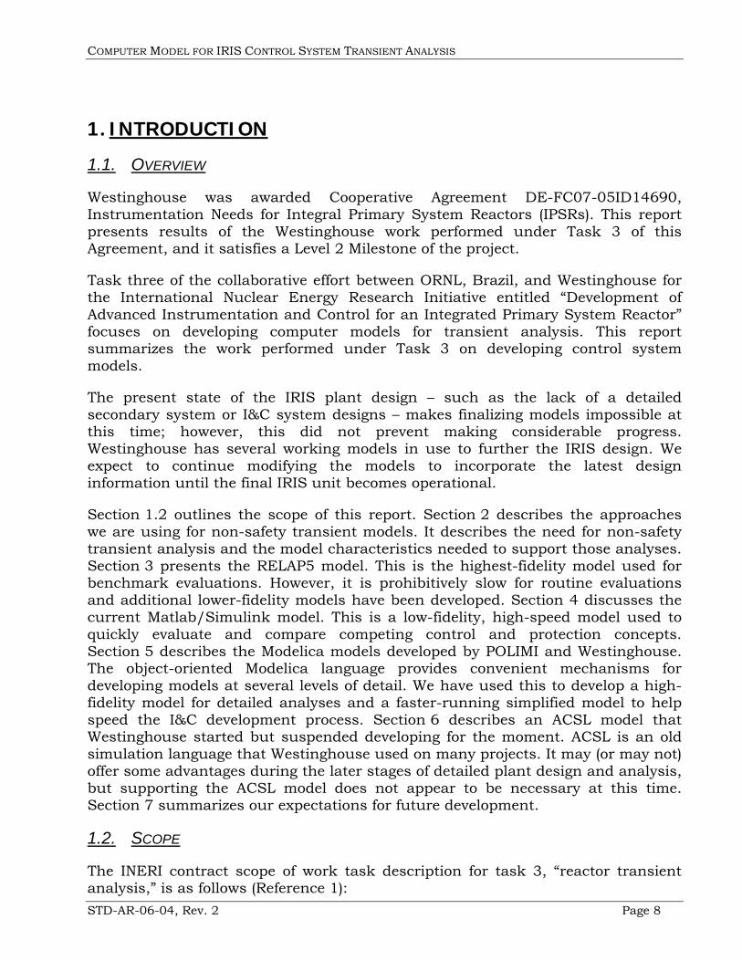
Westinghouse was awarded Cooperative Agreement DE-FC07-05ID14690, Instrumentation Needs for Integral Primary System Reactors (IPSRs). This report presents results of the Westinghouse work performed under Task 3 of this Agreement, and it satisfies a Level 2 Milestone of the project.
Task three of the collaborative effort between ORNL, Brazil, and Westinghouse for the International Nuclear Energy Research Initiative entitled “Development of Advanced Instrumentation and Control for an Integrated Primary System Reactor” focuses on developing computer models for transient analysis. This report summarizes the work performed under Task 3 on developing control system models.
The present state of the IRIS plant design – such as the lack of a detailed secondary system or I&C system designs – makes finalizing models impossible at this time; however, this did not prevent making considerable progress. Westinghouse has several working models in use to further the IRIS design. We expect to continue modifying the models to incorporate the latest design information until the final IRIS unit becomes operational.
Section 1.2 outlines the scope of this report. Section 2 describes the approaches we are using for non-safety transient models. It describes the need for non-safety transient analysis and the model characteristics needed to support those analyses. Section 3 presents the RELAP5 model. This is the highest-fidelity model used for benchmark evaluations. However, it is prohibitively slow for routine evaluations and additional lower-fidelity models have been developed. Section 4 discusses the current Matlab/Simulink model. This is a low-fidelity, high-speed model used to quickly evaluate and compare competing control and protection concepts. Section 5 describes the Modelica models developed by POLIMI and Westinghouse. The object-oriented Modelica language provides convenient mechanisms for developing models at several levels of detail. We have used this to develop a high-fidelity model for detailed analyses and a faster-running simplified model to help speed the I&C development process. Section 6 describes an ACSL model that Westinghouse started but suspended developing for the moment. ACSL is an old simulation language that Westinghouse used on many projects. It may (or may not) offer some advantages during the later stages of detailed plant design and analysis, but supporting the ACSL model does not appear to be necessary at this time. Section 7 summarizes our expectations for future development.
1.2. SCOPE
The INERI contract scope of work task description for task 3, “reactor transient analysis,” is as follows (Reference 1):

COMPUTER MODEL FOR IRIS CONTROL SYSTEM TRANSIENT ANALYSIS
STD-AR-06-04, Rev. 2 Page 9
1. “As part of this task, Westinghouse will review the existing IRIS analytical models and complete their development to be consistent with specific requirements of other tasks in this project. Westinghouse has been developing both detailed IRIS plant models (core physics models and RELAP5 safety analyses plant model) in co-operation with various IRIS partners and low order simulation tools for control systems design and plant dynamic response (MODELICA Plant Simulator in co-operation with POLIMI, Italy).”
This year’s effort was to “complete the development of the IRIS RELAP and MODELICA models as necessary to support other tasks in the project” (Reference 1). This report focuses on the non-safety transient analysis models developed to support the control system design effort. To a lesser degree, these models support the protection system design effort as well, not from a safety perspective, but from a normal operating perspective. This report serves as the task deliverable, namely, “…. report documenting the models and their relationship to the requirements of other tasks in the project” (Reference 1).
COMPUTER MODEL FOR IRIS CONTROL SYSTEM TRANSIENT ANALYSIS
STD-AR-06-04, Rev. 2 Page 10
2. I&C MODELING CONSIDERATIONS
The distinguished statistician George P. E. Box once said, "All models are wrong-but some models are useful." Perhaps no one can agree with this more than someone experienced in developing plant transient analysis models for control system development. Reference 2 identified the need to have dynamic plant models suitable for performing control system analyses and the need to include experienced control system designers who understand the special needs that the model must address as part of the development team.
Reference 2 suggested that the control system design effort requires analyzing transients such as the following:
1. Normal transients
a. Startup transients i. Initial turbine loading
b. Power change transients i. Daily load follow ii. Ramp load changes iii. Step load changes iv. Grid frequency control
c. Shutdown transients
d. Event-based transients i. Startup ↔ main feedwater mode switching ii. Bypass ↔ main feedwater valve iii. One ↔ two main feedwater pumps
2. Abnormal events
a. Approach to protection or operational limits b. Reactor trip c. Turbine trip d. Generator breaker trip e. Switchyard breaker trip f. Islanding g. Turbine fast valving h. Feedwater pump trip i. Reactor coolant pump trip j. Feedwater and condensate train functions k. Miscellaneous functions
We reviewed this list to determine the capabilities that the transient analysis model should have. Most of the listed events involve power operation with essentially

COMPUTER MODEL FOR IRIS CONTROL SYSTEM TRANSIENT ANALYSIS
STD-AR-06-04, Rev. 2 Page 11
identical conditions for all steam generators and for all reactor coolant pumps. A few events start from power operation and proceed to shutdown conditions. The remaining events are listed below, together with the assessment of applicability and suitability of the models described in this report for addressing these events:
1. Item 1.a.i: Initial turbine loading
Although this event does not start from power operation, it should be easy to include the capability for modeling this event.
2. Item 1.b.1: Daily load follow
From an NSSS or turbine perspective, daily load follow is not a severe event. The primary limiting factors are (1) core I-135 and Xe-135 transients and (2) turbine stress limits. Other models provide better tools for addressing these issues.
3. Item 2.i: Reactor coolant pump trip
This event would require a special model that could account for different flows through different steam generators. The models described in this report will not provide the capability to analyze these events.
4. Item 2.j: Feedwater and condensate train functions
These will be accommodated where it makes sense to do so; however, many of them have little impact on whole-plant response, so smaller, more specialized models may be preferred.
5. Item 2.k: Miscellaneous functions
These also will be accommodated where it makes sense to do so; however, many of them have little impact on whole-plant response, so smaller, more specialized models may be preferred.
Control system design involves making a large number of simulation runs. A nuclear power plant design may require tens to hundreds of thousands of runs. Many of these are parametric runs used to optimize individual settings. There are many events to examine, and these may occur at different operating points, each defined by its own powers, pressures, temperatures, and flows. In order to examine all the necessary cases, the models must be simple and must execute quickly.
The approach we are taking on IRIS is to develop a hierarchy of models ranging from fast, low-fidelity models to slower, higher-fidelity models. The detailed models used for accident analysis (e.g., RELAP models) are generally too cumbersome and too slow to be used for effective control system development, but may be used for benchmarking. The emphasis during the second project year was therefore shifted to faster-executing models. The first IRIS model suitable for control studies was the Modelica model developed at POLIMI (Reference 3). We examined this model in
COMPUTER MODEL FOR IRIS CONTROL SYSTEM TRANSIENT ANALYSIS
STD-AR-06-04, Rev. 2 Page 12
2004 and concluded that we needed a faster model. Francesco Schiavo simplified the POLIMI model, increasing its speed by an order of magnitude. The result was the model used for the analyses reported in Reference 4. We have continued to refine the model, and Section 5 describes the current versions.
The simplified Modelica model was (and still is) slower than we would like for rapid prototyping and preliminary control system assessment, so we started developing simpler models. At first we looked at using ACSL, using the models developed for Temelín as a starting point. Traditional ACSL is a text-based language, but the latest version, acslXtreme, has graphical programming capability. ACSL is a good language to use when validating a detailed digital design implementation, but it is less suited to preliminary evaluations when the system designs are still fluid. We decided to place the ACSL model development on hold for the time being. Section 6 discusses ACSL and how an ACSL model might fit into future activities. The alternate that we pursued was Matlab/Simulink. In addition to Simulink, a graphical programming tool well suited for rapid development, Matlab has a number of control system design tools. We developed a Simulink model that emphasized execution speed. Section 4 describes the resulting model.
The models fit together into a coherent plan. We designed the Matlab/Simulink model for rapid prototyping and evaluation. It facilitates easy modification and runs quickly, allowing the control system designer to test and compare various ideas efficiently. The simplified version of the Modelica model provides improved fidelity while remaining relatively easy to modify, but it executes more slowly. The original Modelica model provides even better fidelity, but it runs too slowly for high-volume use. Finally, an ACSL model would give the user precise control over the control system models, including faithful representation of individual software modules and their execution order, but the time required to create such a model would prohibit casual use.
COMPUTER MODEL FOR IRIS CONTROL SYSTEM TRANSIENT ANALYSIS
STD-AR-06-04, Rev. 2 Page 13
3. THE RELAP MODEL
3.1. MODEL OVERVIEW
3.1.1. MODEL PURPOSE
Beside the development of the full plant simulator with Modelica (described later in more detail in Section 5), as part of the original scope of work for this program Westinghouse also performed review and updates to the plant model used for safety analyses based on the RELAP5 computer code (Reference 5).
The high fidelity RELAP model provides accurate simulations of transients. However, its running time may amount to hours or even days and it is thus prohibitive for repetitive simulations of transients needed to optimize control systems and instrumentation designs. Its main purpose instead is for reference and benchmarking analyses.
3.1.2. MODELING ENVIRONMENT
The RELAP5 hydrodynamic model is a one-dimensional, transient, two-fluid model for flow of a two-phase steam-water mixture. The code has been developed and used for the analysis of light water reactors (and also for CANDU analyses) with a loop design. Although the RELAP code has been extensively used in the analyses of light water reactors, and has also been used in the transient analyses of advanced Westinghouse passive plants, the introduction of a new reactor and supporting systems poses great challenges to the development of an appropriate plant representation in RELAP. In particular, the IRIS integral reactor coolant system layout is sufficiently different from the typical loop PWR to require a new approach to develop the coolant system model, based on the best available experience.
3.2. THE MODEL
3.2.1. THE ORIGINAL MODEL
A schematic of the IRIS systems is shown in Figure 1.
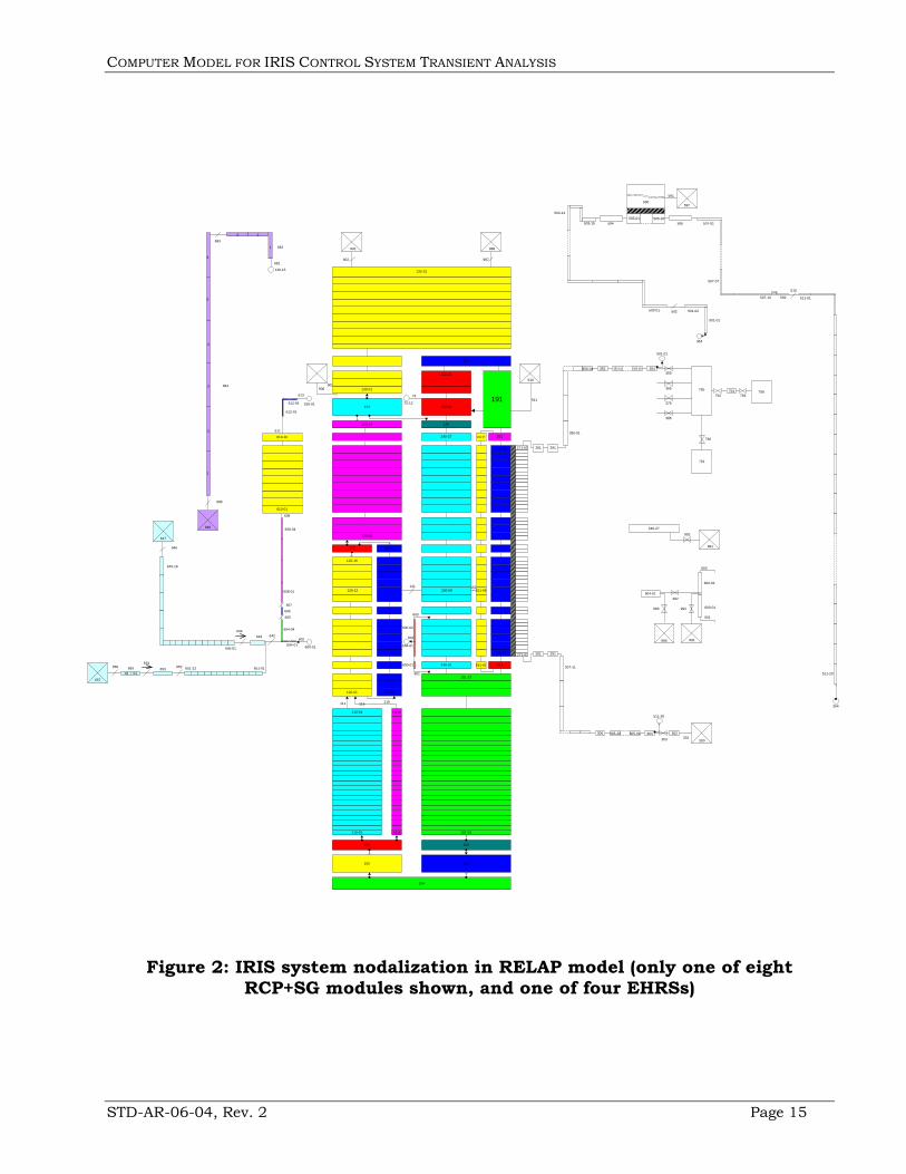
The RELAP representation of the IRIS systems in terms of calculational “nodes” is shown in Figure 2. While the selected structure of the nodalization is simple and is based on the most updated geometrical and operational data available, the discretization of the components is rather detailed in order to take into account all the important phenomena. Most of the calculational nodes have a linear size in the range of 200 to 500 millimeters. In this nodalization volume is always conserved, as well as height due to the importance of natural circulation, so the equivalent flow area is calculated from volume and height.

COMPUTER MODEL FOR IRIS CONTROL SYSTEM TRANSIENT ANALYSIS
STD-AR-06-04, Rev. 2 Page 14
AUX. T.B.BLDG.
Main Steam Line (1 of 4)Isolation Valves
Main Feed Line (1 of 4)Isolation Valves
SGMake
upTank
P/H P/H
P/H P/H
EHRS Heat Exchanger Refueling Water Storage
Tank (1 of 1)
Start Up FeedWater
Steam Generator(1 of 8)
FO FO
SuppressionPool (1 0f 6)
ADS/PORV(1 of 1)
Long Term Core Makeupfrom RV Cavity
(1 of 2)
RCP(1 of 8)
SG Steam Lines(2 of 8)
SG FeedWater Lines
(2 of 8)
FO FO
SafetyValve
SafetyValve
RV Cavity
SuppressionPool Gas
Space
IntegralReactorVessel
Emergency Heat RemovalSystem (EHRS)
1 of 4 Subsystems
DVI
EBT(1 0f 2)
Figure 1: Schematic of the IRIS systems
In general, the IRIS plant RELAP model has been developed over a period of several years, with an overall effort of the order of several man years (see for example References 6-8). The objectives of the review performed as part of this program were as follows:
1. Consolidate various version of the IRIS plant model in a single model, including updated models of different components;
2. Review existing analyses of design basis and beyond design basis sequences to identify where plant (and thus model) modifications were necessary to optimize the plant response;
3. Review the most up to date plant design documentation and identify those areas where an update to the simulation model was necessary.
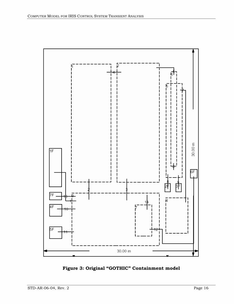
While the original scope only included the RELAP5 computer code, the full safety analysis simulator for IRIS is composed of RELAP5 for the primary and secondary systems and GOTHIC (Reference 9) for the containment. Therefore performing a review only of the RELAP5 model was not considered sufficient and the complete plant model (RELAP5 and GOTHIC) was reviewed. The original GOTHIC model is shown in Figure 3.
COMPUTER MODEL FOR IRIS CONTROL SYSTEM TRANSIENT ANALYSIS
STD-AR-06-04, Rev. 2 Page 15
Figure 2: IRIS system nodalization in RELAP model (only one of eight RCP+SG modules shown, and one of four EHRSs)
101-27
102
103
104
105
106
121-01
111 116 119
221
211-01
211-25
121-17122
201
240-01
240-27 241-27
241-01
601
600-01
600-02
603
124
125
150-01
150-04
151
271-50
271-01 251261
281 291
350-01
350-04 352 353-01 353-08 354355
501-01
501-02502503-01
503-12
503-15 504505-01 505-20
506 507-01
507-07
507-10508
509
510
511-01
307-11
750
590
591
592
141 161211-08
906905
992993
604-01
602
72-12
73
110-01
110-24
115-01
115-24
123-01
123-14
130-01
101-01
305-20 305-01 304
303 300
306 302301
354
501-01
511-20
130-15
902
901
987
988
120-01
511-20
304
375
365
385
754752 756
758
761
760
120-16
240-09120-12
911
910
191
600-01
610-01
610-10
604-01
604-04
605
606
607
608-01
608-04
609
611
612-01
612-04 150-01
602
613
682
683
684
2
1
3
686
685
681
130-15
6
2
1
3
4
5
642643644
645-16
647
646
651-01652653
654655656
657
645-01
0102651-12
602
991
604-01
995
601
600-01
600-02
603
240-27
991
992
COMPUTER MODEL FOR IRIS CONTROL SYSTEM TRANSIENT ANALYSIS
STD-AR-06-04, Rev. 2 Page 16
Figure 3: Original “GOTHIC” Containment model
COMPUTER MODEL FOR IRIS CONTROL SYSTEM TRANSIENT ANALYSIS
STD-AR-06-04, Rev. 2 Page 17
3.2.2. MODEL REVIEW AND MODIFICATIONS
The RELAP model has been reviewed with the objective to identify revisions needed to reflect the most recent/updated IRIS design features and parameters as well as to make it more suitable for benchmarking the transient analyses that will be performed as part of this project using the low-order Modelica model(s).
The review of the RELAP model focused on those changes that may potentially impact the system response and, thus, need to be evaluated from the standpoint of their impact on modeling the control system. This included the following IRIS system features and components:
• Emergency boration tank (EBT), automatic depressurization system (ADS), pressure suppression system (PSS), and long term gravity makeup system (LGMS).
• Emergency Heat Removal System (EHRS) condenser design details (number of tubes, tube geometry).
• Refueling Water Storage Tank (RWST) elevation, which will reflect Reactor Coolant System (RCS) elevation modification in order to provide adequate natural circulation head for the EHRS.
• RCS elevation within the containment building in order to optimize the layout of the main system piping and of the auxiliary systems housed in the reactor containment building as well as the main system piping routing in order to optimize the system response in both normal and emergency operation.
Result of this review is summarized in the following sub-sections
3.2.2.1 REVIEW OF EBT, ADS AND LGMS MODEL
The review confirmed that the original sizing of the main safety systems provided an acceptable and adequate response to all design basis conditions, and no update was, therefore, required to the design and modeling of the following systems: EBT, ADS, PSS, and LGMS.
3.2.2.2 REVIEW AND MODIFICATIONS OF THE CONTAINMENT LAYOUT MODEL
The design evolution has lead to modifications in the original design that required updating the plant model. The most relevant changes were required as a consequence of the updated containment layout. Detailed design activities performed during the past few years have provided a more complete design of the IRIS containment system. In particular, concerns were identified related to the reduced size of the containment with respect to the need to include all the necessary equipment. In particular, it was necessary to re-arrange the pressure suppression system, which in now composed of a low elevation suppression pool (the true “pressure suppression system”) plus a connected upper tank with a function to provide early water injection by gravity to respond to certain beyond
COMPUTER MODEL FOR IRIS CONTROL SYSTEM TRANSIENT ANALYSIS
STD-AR-06-04, Rev. 2 Page 18
design scenarios, such as multiple failures assumed on the emergency heat removal system. This second tank has been named the “long term gravity makeup tank” (LGMT). Corresponding modifications have been made to the model.
3.2.2.3 REVIEW AND MODIFICATIONS OF THE EHRS MODEL
Particular attention was given to the review of the performance (and model) of the EHRS due to its importance for the long term cooling of the plant. The effect on its response due to a variation of the system mass inventory was evaluated, and the results are reported below.
The EHRS is a passive emergency heat removal system consisting of four independent subsystems each of which has a U-tube condenser placed in the RWST connected to a train of two Steam Generators (SG). The EHRS provides both the main post Loss of Coolant Accident (LOCA) depressurization of the primary system and the coolant makeup function to the primary system. EHRS operates on natural circulation removing heat from the primary system through the SG surface and rejecting the absorbed heat to the RWST through the U-tube condensers.
The performance of any closed two-phase thermo-siphon, like the EHRS, depends on many variables, among these the system mass content (the total mass of fluid within the system) being among the most important. The EHRS mass inventory variations analyzed span the range of possible system modifications, such as piping routing and components elevations, and also reflect more control related issues, such as isolation valve closing time. The EHRS mass content is represented through the so called Filling Ratio, defined as the ratio of the mass the system actually contains to the maximum amount of mass it could contain if it were completely filled.
The IRIS RELAP was modified and several simulations were performed to evaluate impact of different filling ratios. A representative selection of the results obtained is presented in Figure 4 through Figure 6.

COMPUTER MODEL FOR IRIS CONTROL SYSTEM TRANSIENT ANALYSIS
STD-AR-06-04, Rev. 2 Page 19
Figure 4—EHRS extracted power versus filling ratio
Figure 5—EHRS operating pressure versus filling ratio
COMPUTER MODEL FOR IRIS CONTROL SYSTEM TRANSIENT ANALYSIS
STD-AR-06-04, Rev. 2 Page 20
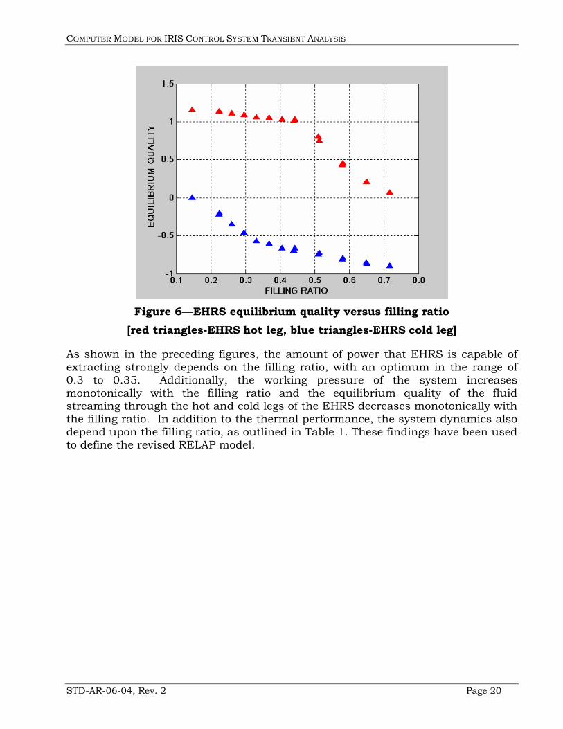
Figure 6—EHRS equilibrium quality versus filling ratio
[red triangles-EHRS hot leg, blue triangles-EHRS cold leg]
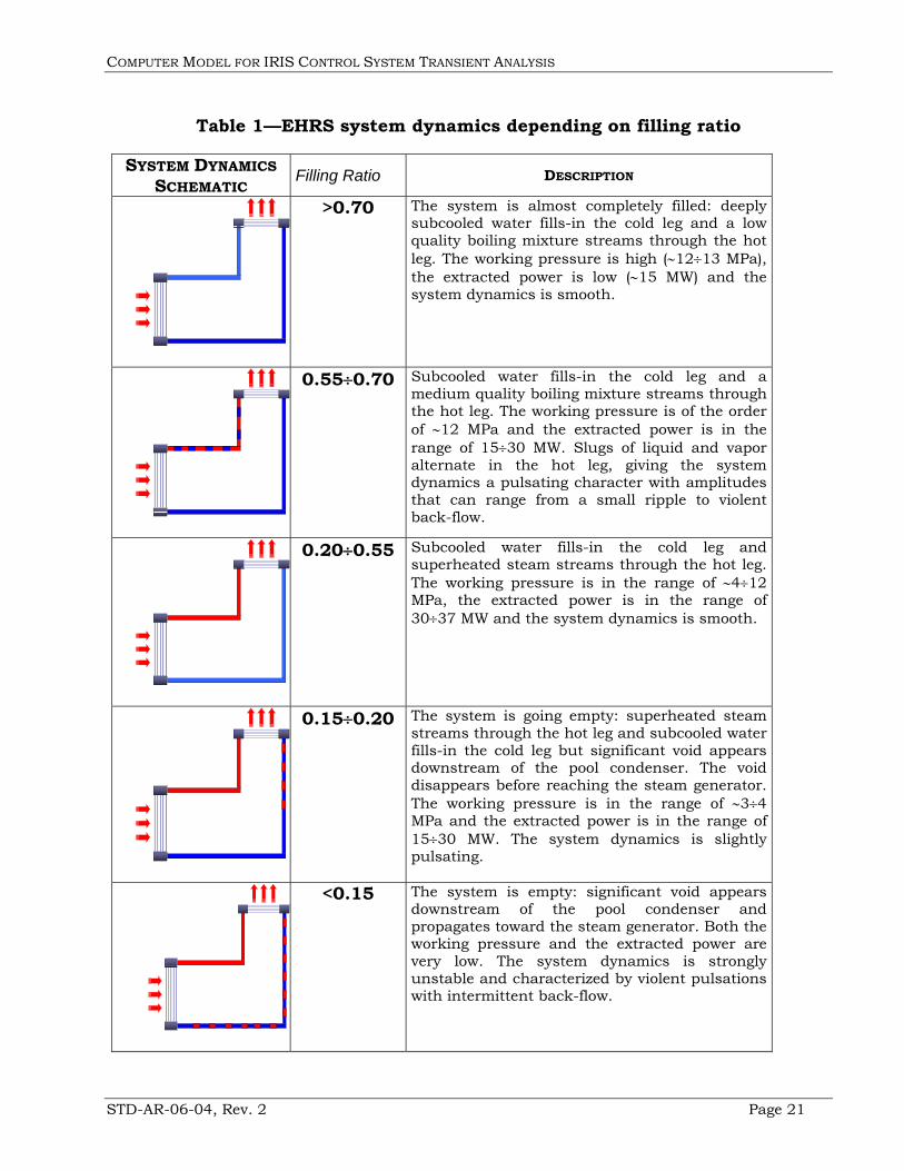
As shown in the preceding figures, the amount of power that EHRS is capable of extracting strongly depends on the filling ratio, with an optimum in the range of 0.3 to 0.35. Additionally, the working pressure of the system increases monotonically with the filling ratio and the equilibrium quality of the fluid streaming through the hot and cold legs of the EHRS decreases monotonically with the filling ratio. In addition to the thermal performance, the system dynamics also depend upon the filling ratio, as outlined in Table 1. These findings have been used to define the revised RELAP model.
COMPUTER MODEL FOR IRIS CONTROL SYSTEM TRANSIENT ANALYSIS
STD-AR-06-04, Rev. 2 Page 21
Table 1—EHRS system dynamics depending on filling ratio
SYSTEM DYNAMICS SCHEMATIC Filling Ratio DESCRIPTION
>0.70 The system is almost completely filled: deeply subcooled water fills-in the cold leg and a low quality boiling mixture streams through the hot leg. The working pressure is high (∼12÷13 MPa), the extracted power is low (∼15 MW) and the system dynamics is smooth.
0.55÷0.70 Subcooled water fills-in the cold leg and a medium quality boiling mixture streams through the hot leg. The working pressure is of the order of ∼12 MPa and the extracted power is in the range of 15÷30 MW. Slugs of liquid and vapor alternate in the hot leg, giving the system dynamics a pulsating character with amplitudes that can range from a small ripple to violent back-flow.
0.20÷0.55 Subcooled water fills-in the cold leg and superheated steam streams through the hot leg. The working pressure is in the range of ∼4÷12 MPa, the extracted power is in the range of 30÷37 MW and the system dynamics is smooth.
0.15÷0.20 The system is going empty: superheated steam streams through the hot leg and subcooled water fills-in the cold leg but significant void appears downstream of the pool condenser. The void disappears before reaching the steam generator. The working pressure is in the range of ∼3÷4 MPa and the extracted power is in the range of 15÷30 MW. The system dynamics is slightly pulsating.
<0.15 The system is empty: significant void appears downstream of the pool condenser and propagates toward the steam generator. Both the working pressure and the extracted power are very low. The system dynamics is strongly unstable and characterized by violent pulsations with intermittent back-flow.
COMPUTER MODEL FOR IRIS CONTROL SYSTEM TRANSIENT ANALYSIS
STD-AR-06-04, Rev. 2 Page 22
3.2.2.4 REVIEW AND MODIFICATIONS OF THE RWST MODEL
The RWST pool and the EHRS heat exchanger were originally located at approximately 10 m above the steam line. A seismic design review has identified benefits of lowering this large body of water. Therefore, the impact of the RWST elevation was examined. It was found that this elevation may be notably reduced, as long as a certain minimum axial separation to steam lines is maintained, and the EHRS is modified accordingly. EHRS performance studies were carried out to identify that necessary size increase needed to compensate for the reduction of the heat exchanger elevation to about 1m above the steam lines. It was found that an increase of approximately 10% in the heat exchanger tubes is adequate. This modification has been reflected in the revised RELAP5 model.
Elevation of the RCS and routing of piping has been assessed as well, but it was found unpractical to revise the model before the final containment layout design becomes available.
3.2.2.5 MODEL MODIFICATIONS RELATED TO BEYOND DESIGN BASIS SCENARIOS
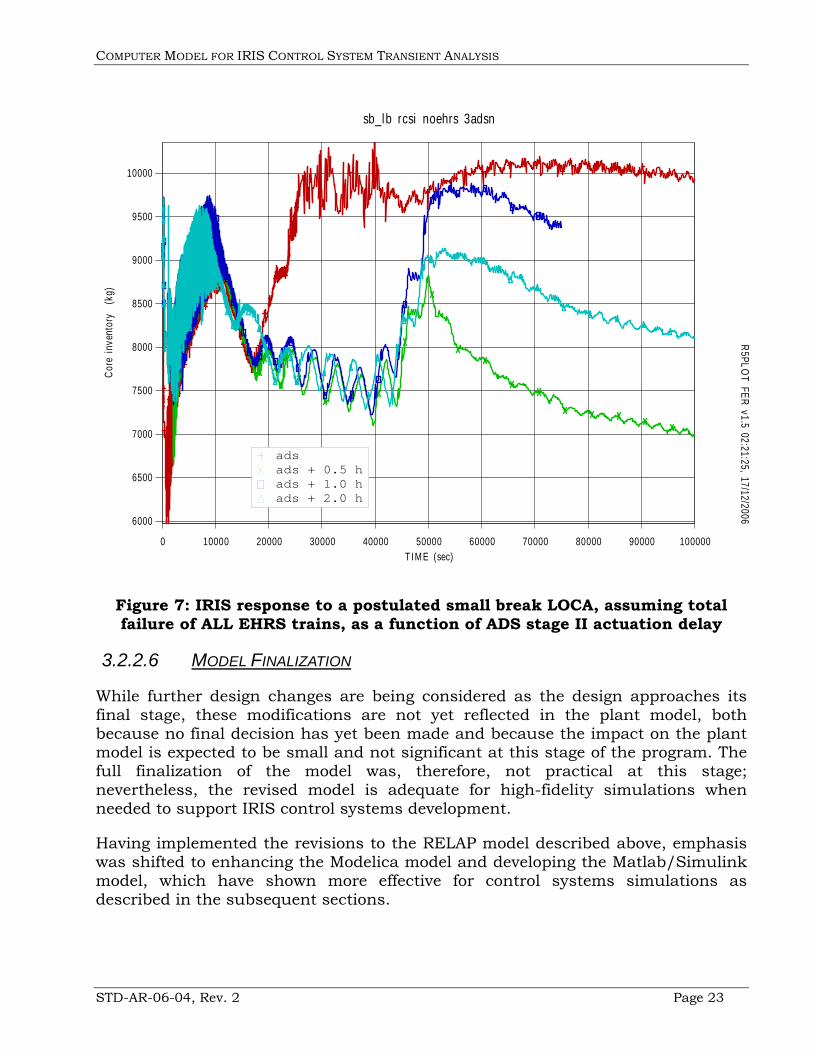
A final set of changes was implemented to improve the IRIS response to certain beyond design basis conditions. A specific PRA sequence was identified (Reference 10) as the key beyond design basis condition for which an effective system response was necessary. This sequence involves the postulated complete failure of the EHRS (all four trains) following a postulated loss of coolant accident. In this case, the IRIS mitigation strategy would be based on the ADS (to vent steam generated in the core by decay heat) and the passive containment cooling system (PCCS). To improve the plant response in this configuration, it was identified that two changes were necessary:
1. Increase in the size of the ADS, which has been achieved by adding a second stage ADS. This modification has been reflected in an updated version of the RELAP5 model and of the safety systems functional diagram.
2. Optimization of the actuation logic of the PCCS and the ADS, which has been achieved by introducing a delay in the ADS actuation. This delay ensures that the containment is not completely depressurized until certain conditions are met and verified by the operator. A sequence of simulations was performed to study the impact of timing delays in actuating the second stage of the ADS system. Figure 7 shows the effect of 3 selected actuation delays on the core inventory. These results will be used to finalize the model once all other design details have been defined.
COMPUTER MODEL FOR IRIS CONTROL SYSTEM TRANSIENT ANALYSIS
STD-AR-06-04, Rev. 2 Page 23
Figure 7: IRIS response to a postulated small break LOCA, assuming total failure of ALL EHRS trains, as a function of ADS stage II actuation delay
3.2.2.6 MODEL FINALIZATION
While further design changes are being considered as the design approaches its final stage, these modifications are not yet reflected in the plant model, both because no final decision has yet been made and because the impact on the plant model is expected to be small and not significant at this stage of the program. The full finalization of the model was, therefore, not practical at this stage; nevertheless, the revised model is adequate for high-fidelity simulations when needed to support IRIS control systems development.
Having implemented the revisions to the RELAP model described above, emphasis was shifted to enhancing the Modelica model and developing the Matlab/Simulink model, which have shown more effective for control systems simulations as described in the subsequent sections.
0 10000 20000 30000 40000 50000 60000 70000 80000 90000 100000T IM E (sec)
Core
inve
ntor
y (
kg)
6000
6500
7000
7500
8000
8500
9000
9500
10000
ads ads + 0.5 h ads + 1.0 h ads + 2.0 h
sb_lb rcsi noehrs 3adsn
R5PLOT FER v1.5 02:21:25, 17/12/2006

COMPUTER MODEL FOR IRIS CONTROL SYSTEM TRANSIENT ANALYSIS
STD-AR-06-04, Rev. 2 Page 24
4. THE MATLAB/SIMULINK MODEL
4.1. MODEL OVERVIEW
4.1.1. MODEL PURPOSE
Our Matlab/Simulink IRIS model sits at the lowest level of the project’s model hierarchy. We designed our model for rapid prototyping and initial design evaluation, not for detailed, accurate analyses. We deliberately sacrificed detail in exchange for execution speed and model flexibility. Our purpose was to write a model that would give control system designers a tool to rapidly evaluate competing control system design concepts and determine which ones hold the most promise for more detailed development and evaluation. This philosophy is evident in the simplifying assumptions we made throughout the model.
The Matlab/Simulink environment facilitates easy model modification. Our model runs quickly, allowing the control system designer to test and compare various alternatives efficiently.
4.1.2. MODELING ENVIRONMENT
Matlab/Simulink provides a graphical modeling environment that includes expandable libraries of predefined blocks and an interactive graphical editor for assembling and managing intuitive block diagrams. It gives the modeler the ability to manage complex designs by segmenting models into hierarchies of design components. As we see it, the key strength of the Matlab/Simulink environment is the way it allows for rapid model development, while its weakness lies in the difficulty of modeling extremely complex systems while maintaining precise control over all components, particularly with respect to how and in what order Matlab/Simulink solves equations. A drawback is that the modeling environment continuously pauses, apparently to check the connection with the license server. Response delays of up to seven minutes are commonplace, particularly at the beginning of each session.

COMPUTER MODEL FOR IRIS CONTROL SYSTEM TRANSIENT ANALYSIS
STD-AR-06-04, Rev. 2 Page 25
4.2. THE MODEL
4.2.1. HIGH-LEVEL STRUCTURE
4.2.1.1 MODEL COMPONENTS
Turbine tripped
0Turbine Trip
Ppzr
Psh ref
Wf w
Wrcs
TestDisturbances
Test Disturbances
10Start time
0Simulation Time
sensor
sensor
sensor
sensor
sensor
sensor
sensor
sensor
sensor
sensor
sensor
Reactor tripped
0Reactor Trip
Flow Dist [frac IC]
Reactor trip [bool]
Turbine trip [bool]
Pzr controls
Rod Speed Demand [steps/s]
Wfw Dem [frac]
Steam dump demand [frac]
TV demand [frac]
Grid Connection
Qn [frac]
Feedwater flow [frac]
Thot; Tcold [C; C]
Pzr Pressure [Pa]
Vpzr liq [frac]
SG level [frac]
Steamheader pressurer [Pa]
Turbine steam flow [frac]
Gen power [frac]
Gen freq [Hz]
Plant
0MWreq
0MWref
MW output request [f rac]
MW load change [f rac]
Request ElectricPower Transient
0MWe
MWreq [frac]MWe [frac]Qn [frac]Qtu [frac]Thot [C]Tcold [C]Ppzr [Pa]Vpzr liq [frac]Ps [Pa]Wfw [frac]Frequency [Hz]Lsg [frac]Ppzr ref Psh ref disturbanceWfwref disturbanceTrip Reactor [bool]Trip Turbine [bool]
MWref [frac]
Rx & T Trip
Tref & DB [C]
Tavg [C]
Pref [Pa]
Pzr controls
Rod Speed [step/m]
Rod Speed [step/s]
Wfw demand [frac]
SDdem [frac]
TVdem [frac]
I&CSystems
[Vliq]
[Ppzr]
[freq]
[Wfwn]
[Qgen]
[Wsn]
[Psh]
[dMWload]
[WrcsDist]
[Lsg]
[Qn]
[ThTc][Vliq]
[Qgen]
[Ppzr]
[freq]
[Wfwn]
[Qgen]
[Wsn]
[Psh]
[dMWload]
[WrcsDist]
[Lsg]
[Qn]
[ThTc]
Qgen [f rac]
Load change [f rac]
Freq [Hz]
Max load [f rac]
Max load IC
Grid ModelFinite grid
Finite Grid
0Event Time
false
Constant1
true
Constant
Clock
TVdem
Wf wdem
Wf w
Tref DBs
Qn meas
Qtu meas
Th meas
Tc measTav g
Psh meas
RodSpeed
Th;Tc
Qn
Pref
MWe meas
Wf w meas
f meas
MWref
SDdem
Ppzr
Ppzr meas
Vpzr liq
Vliq meas
Reactor trip
LsgLsg meas
Qgen
Qgen
Psh
Wsn
Freq
f requency
Max Load
Max Load IC
Turbine trip
Figure 8: Matlab/Simulink root-level model
Figure 8 shows the root-level view of the Matlab/Simulink IRIS model. The model has the following major blocks:
1. Plant Block
The plant block includes all of the modeled plant mechanical components, including the reactor, primary system, secondary system, turbine, and generator. Most of the inputs are plant control signals. These will change as the I&C system evolves. The grid connection input provides grid feedback, most notably via grid frequency. The flow disturbance input is a code-control input that provides a convenient way to examine the effect of steam flow disturbances. Most of the plant outputs are measured process variables. The plant model also puts out generator power to support the grid model. Section 4.2.2 describes the plant model in more detail.
2. Grid model
The grid model has two inputs: generator power output and a code control signal used to cause a change in grid load. The outputs are

COMPUTER MODEL FOR IRIS CONTROL SYSTEM TRANSIENT ANALYSIS
STD-AR-06-04, Rev. 2 Page 26
the grid frequency and the maximum power that the grid can accept from the unit (this limit comes from plant and grid impedances). Section 4.2.2.3.2 describes the grid model in more detail.
3. I&C Systems model
The I&C Systems model includes the control and protection system models. The inputs fall into the following four categories:
A. Sensor signals. The specific signals will change as the I&C system design progresses.
B. Initial conditions. This version of the model allows the user to start with the reactor and turbine tripped.
C. Disturbances. These artificial signals provide a convenient way to evaluate control system responses to selected disturbances.
D. Code control signals. These are signals used to define which transient to analyze. In this version of the model, the signal used is the requested electric power output.
The remaining components shown in Figure 8 fall into three categories. The first category is sensor models. The current sensor model implements sensor high and low limits and a sensor response time. The decision to place the sensors on the root-level diagram was arbitrary. The second category is user interface components. See Section 4.2.1.2 for more information on these. The final category is minor components used for signal routing; these enhance the readability of the diagram.
4.2.1.2 USER INTERFACE
Before running a simulation, the user must initialize the model. Many model variables depend on the initial power. For convenience, we have standard scripts (m-files) that initialize all necessary model variables. Once the script has run, the user may analyze any number of transients starting from the same initial conditions.
The normal method for obtaining output is to use the Simulink Signal & Scope Manager, which provides considerable flexibility in plotting simulation results.
As noted in the previous section, Figure 8 provides the main user interface to the model. The major interface components shown on Figure 8 are as follows:
1. The “Requested Electric Power Transient” block is where the user defines the desired event. Double-clicking brings up the following interface screen (“Never” is a global variable defined in the initialization scripts):
COMPUTER MODEL FOR IRIS CONTROL SYSTEM TRANSIENT ANALYSIS
STD-AR-06-04, Rev. 2 Page 27
Figure 9: Current transient definition screen
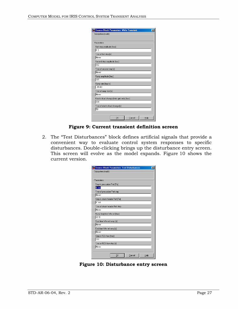
2. The “Test Disturbances” block defines artificial signals that provide a convenient way to evaluate control system responses to specific disturbances. Double-clicking brings up the disturbance entry screen. This screen will evolve as the model expands. Figure 10 shows the current version.
Figure 10: Disturbance entry screen
COMPUTER MODEL FOR IRIS CONTROL SYSTEM TRANSIENT ANALYSIS
STD-AR-06-04, Rev. 2 Page 28
3. “Reactor tripped” and “Turbine tripped” switches. These switches allow starting the run with the reactor and/or turbine tripped.
4. Overview displays. There are three summary display groups. The first, in yellow at the top right of Figure 8, monitors the run progress. The second, to the left of the first and in yellow as well, shows various electric power signals. We use this as a quick check on proper run progress. The third set of displays, in orange, indicates whether the reactor and/or turbine tripped during the simulation.
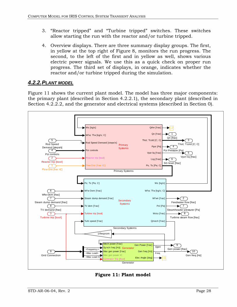
4.2.2. PLANT MODEL
Figure 11 shows the current plant model. The model has three major components: the primary plant (described in Section 4.2.2.1), the secondary plant (described in Section 4.2.2.2, and the generator and electrical systems (described in Section 0).
10Gen freq [Hz]
9Gen power [frac]
8Turbine steam flow [frac]
7Steamheader pressurer [Pa]
6SG level [frac]
5Vpzr liq [frac]
4Pzr Pressure [Pa]
3Thot; Tcold [C; C]
2Feedwater flow [frac]
1Qn [frac]
Ps; Ts [Pa; C]
Wf w Dem [f rac]
Steam dump demand [f rac]
TV dem [f rac]
Turbine trip [bool]
Turb speed [f rac]
Ws [kg/s]
Wf w; Tf w [kg/s; C]
Wf wn [f rac]
Psl [Pa]
Wstu [f rac]
Qmech [f rac]
SecondarySystems
Secondary Systems
Ws [kg/s]
Wf w; Tf w [kg/s; C]
Rod Speed Demand [steps/s]
Pzr controls
Reactor trip [bool]
Flow Dist [f rac IC]
Qthn [f rac]
Qn [f rac]
Thot; Tcold [C; C]
Ppzr [Pa]
Vpzr liq [f rac]
Lsg [f rac]
Ps; Ts [Pa; C]
PrimarySystems
Primary Systems
Mech power [f rac]Sy nch f req [Hz]
Max gen power [f rac]
Max gen power IC
Generator Trip [Bool]
Gen Power [f rac]
Gen f req [Hz]
Elec Angle [deg]
Generator
Generator
1/freqnom
9Grid Connection
8TV demand [frac]
7Steam dump demand [frac]
6Wfw Dem [frac]
5Rod Speed
Demand [steps/s]4
Pzr controls
3Turbine trip [bool]
2Reactor trip [bool]
1Flow Dist [frac IC]
Freq
Qgen<f requency >
<Max Load>
<Max Load IC>
Figure 11: Plant model

COMPUTER MODEL FOR IRIS CONTROL SYSTEM TRANSIENT ANALYSIS
STD-AR-06-04, Rev. 2 Page 29
4.2.2.1 PRIMARY SYSTEMS
Figure 12 shows the primary systems model. The model consists of the following five parts:
1. The reactor coolant thermal hydraulic model, described in Section 4.2.2.1.2
2. The reactor power model, described in Section 4.2.2.1.1.
3. The rod drive model. This converts rod speed into rod position. The current model assumes that the rod drive mechanism is a stepping mechanism.
4. The reactor coolant pump model. The current model simply models flow changes as a step filtered by a first-order lag. Most control system transient analyses can assume constant reactor coolant pump flow (with the obvious exception of loss of reactor coolant pumps). There is little need for a more detailed model unless one moves to a multi-pump primary model.
5. The pressurizer auxiliaries model. This converts variable and on/off heater demand signals into total pressurizer heater power while accounting for the heater thermal time constant. It also converts relief flow demand to flow in engineering units. For IRIS, this models the pressurizer safety valves since there are no power-operated relief valves.
7Ps; Ts [Pa; C]
6Lsg [frac]
5Vpzr l iq [frac]
4Ppzr [Pa]
3Thot; Tcold [C; C]
2Qn [frac]
1Qthn [frac]
-C-TinIC
[step/s] [SWD]Rod DriveMechanism
Rod Drive
Tcore water [C]
Rod Position [SWD]
Reactor trip [bool]
Thermal Power [W]
Neutron f lux [f rac]
Thermal Power IC [W]
Reactor Power
Reactor Power Model
Rx Power [W]Rx Power IC [W]
Steam f low [kg/s]FW Flow [kg/s]FW Temp [C]
Mass Flow [kg/s]Mass Flow IC [kg/s]Pzr Heater Power [W]
Pzr relief [kg/s]Tin IC [C}
Tcw [C]
Thot [C]
Tcold [C]
Ps [Pa]
Ts [C]
Ppzr [Pa]
Vpzr liq [f rac]
Lsg [f rac]
Reactor Coolant System Thermal Hydraulics
Reactor Coolant System
Flow [f rac IC]
Flow IC [kg/s]Flow [kg/s]
RCPs
RCPs
1/Qcorenom
Prop Htr Dem [f rac]Backup Htr Dem [bool]
Relief Dem [bool]
Pzr Heater Power [W]
Pzr relief [kg/s]
Pzr Systems
Pressurizer Systems
WrcsIC
6Flow Dist [frac IC]
5Reactor trip [bool]
4Pzr controls
3Rod Speed Demand [steps/s]
2Wfw; Tfw [kg/s; C]
1Ws [kg/s]
Tcw
Tcw
TsTs
RodPos
Ps Ps
Thot
Tcold
Qthn
Qn
Ppzr
Figure 12: Primary systems
COMPUTER MODEL FOR IRIS CONTROL SYSTEM TRANSIENT ANALYSIS
STD-AR-06-04, Rev. 2 Page 30
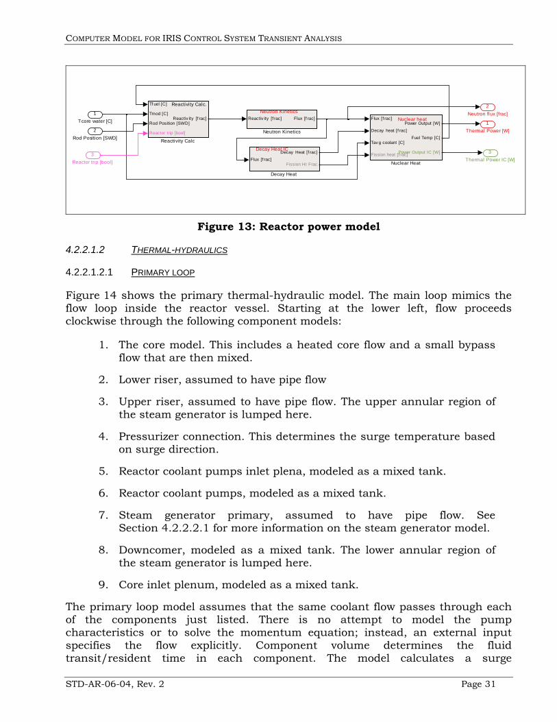
4.2.2.1.1 REACTOR POWER
Figure 13 shows the reactor power model. The model takes moderator temperature and rod position as inputs, and calculates core thermal power and neutron flux. The model consists of the following four parts:
1. Reactivity calculation
The reactivity calculation assumes that reactivity is zero at the start of the simulation. The model accounts for the following three mechanisms for reactivity changes:
A. Fuel temperature changes. The reactivity effect is primarily due to the Doppler temperature effect. The nuclear heat model provides the bulk fuel temperature. In practice, this reactivity term stabilizes the core, but the precise value of the Doppler coefficient has little effect on most transients used in control analyses.
B. Moderator temperature changes. The current model assumes a constant moderator temperature coefficient.
C. Rod position changes. The current model accounts for rod worth as a function of position. The model treats multiple banks operating in a prescribed sequence as one (long) bank. Modeling more complicated operating strategies such as MSHIM would require straightforward extensions to the model.
The model does not include reactivity changes due to xenon-135 transients. Xenon-135 transients should not have a significant effect for the short-term transients that we plan to analyze with this model.
2. Neutron kinetics
The neutron kinetics model is a standard point kinetics model with six delayed neutron groups. It ignores prompt neutron dynamics because they occur too quickly to affect the main variables of interest.
3. Decay heat
The decay heat model incorporates five decay heat groups. It also calculates the total decay heat fraction for the nuclear heat model to use.
4. Nuclear heat model
The nuclear heat model combines the fission and decay heat sources and calculates mean neutron flux, effective fuel temperatures, and heat transfer to the coolant. The model accounts for the small heat fraction generated directly in the coolant.
COMPUTER MODEL FOR IRIS CONTROL SYSTEM TRANSIENT ANALYSIS
STD-AR-06-04, Rev. 2 Page 31
3Thermal Power IC [W]
2Neutron flux [frac]
1Thermal Power [W]
Tf uel [C]
Tmod [C]
Rod Position [SWD]
Reactor trip [bool]
Reactiv ity [f rac]
Reactivity Calc.
Reactivity Calc
Flux [f rac]
Decay heat [f rac]
Tav g coolant [C]
Fission heat [f rac]
Power Output [W]
Fuel Temp [C]
Power Output IC [W]
Nuclear heat
Nuclear Heat
Reactiv ity [f rac] Flux [f rac]Neutron Kinetics
Neutron Kinetics
Flux [f rac]
Decay Heat [f rac]
Fission Ht Frac
Decay Heat IC
Decay Heat
3Reactor trip [bool]
2Rod Position [SWD]
1Tcore water [C]
Figure 13: Reactor power model
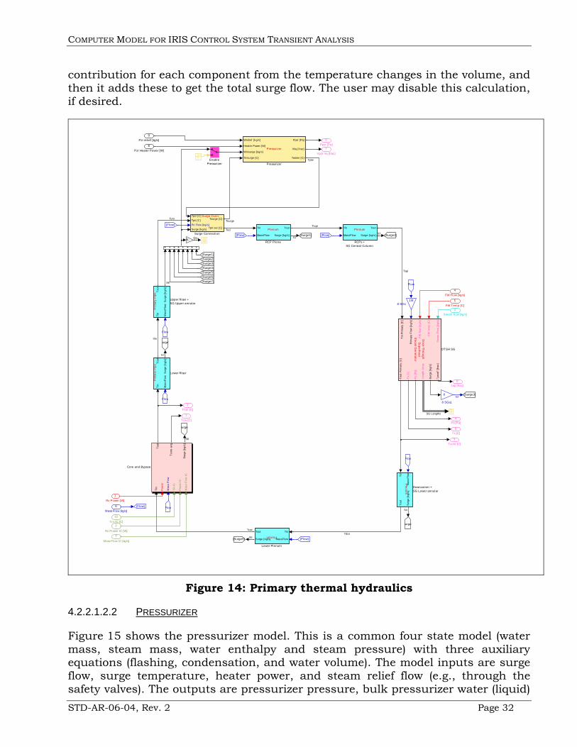
4.2.2.1.2 THERMAL-HYDRAULICS
4.2.2.1.2.1 PRIMARY LOOP
Figure 14 shows the primary thermal-hydraulic model. The main loop mimics the flow loop inside the reactor vessel. Starting at the lower left, flow proceeds clockwise through the following component models:
1. The core model. This includes a heated core flow and a small bypass flow that are then mixed.
2. Lower riser, assumed to have pipe flow
3. Upper riser, assumed to have pipe flow. The upper annular region of the steam generator is lumped here.
4. Pressurizer connection. This determines the surge temperature based on surge direction.
5. Reactor coolant pumps inlet plena, modeled as a mixed tank.
6. Reactor coolant pumps, modeled as a mixed tank.
7. Steam generator primary, assumed to have pipe flow. See Section 4.2.2.2.1 for more information on the steam generator model.
8. Downcomer, modeled as a mixed tank. The lower annular region of the steam generator is lumped here.
9. Core inlet plenum, modeled as a mixed tank.
The primary loop model assumes that the same coolant flow passes through each of the components just listed. There is no attempt to model the pump characteristics or to solve the momentum equation; instead, an external input specifies the flow explicitly. Component volume determines the fluid transit/resident time in each component. The model calculates a surge
COMPUTER MODEL FOR IRIS CONTROL SYSTEM TRANSIENT ANALYSIS
STD-AR-06-04, Rev. 2 Page 32
contribution for each component from the temperature changes in the volume, and then it adds these to get the total surge flow. The user may disable this calculation, if desired.
8Lsg [frac]
7Vpzr l iq [frac]
6Ppzr [Pa]
5Ts [C]
4Ps [Pa]
3Tcold [C]
2Thot [C]
1Tcw [C]
Tin
Mas
sFlo
w
Tou
t
Sur
ge [k
g/s]
Prim
ary
Pip
e
Upper Riser +SG Upper annular
Tpzr [C]
Tpri [C]
Pri Flow [kg/s]
Surge [kg/s]
Tsurge [C]
Tpri out [C]
Surge Conn.
Surge Connection
Tin
MassFlow
Tout
Surge [kg/s]
Plenum
RCPs +SG Central Column
Tin
MassFlow
Tout
Surge [kg/s]
Plenum
RCP Plena
Wrelief [kg/s]
Heater Power [W]
Winsurge [kg/s]
Tinsurge [C]
Ppzr [Pa]
Vliq [f rac]
Twater [C]
Pressurizer
Pressurizer
Tin
Prim
ary
[C]
Prim
ary
Flow
[kg/
s]
FW fl
ow [k
g/s]
FW te
mp
[C]
Ste
am F
low
[kg
/s]
Tout
Prim
ary
[C]
Ts [c
]
Ps [P
a]
Leng
th A
rray
Surg
e [k
g/s]
"Lev
el"
[fra
c]
Once-ThroughS
uperheatS
team G
enerator
OTSH SG
Tin
Mas
sFlo
w
Tou
t
Surg
e [k
g/s]
Prim
ary
Pip
e
Lower Riser
Tin
MassFlow
Tout
Surge [kg/s]
Plenum
Lower Plenum
Surge7
Surge6
[Surge5]
Surge4
[Surge3]
[Surge2]
[Flow]
[Surge1]-K-
[Surge2][Surge1]
Flow
[Flow]
Flow
Flow
[Flow]
Flow
[Flow]
[Surge7][Surge6][Surge5][Surge4][Surge3]
Flow
[Flow]
EnablePressurizer
Tin
Mas
sFlo
w
Tout
Surg
e [k
g/s]
Plenum
Downcomer +SG Lower annularTi
n
Pow
er
Mas
s Fl
ow
Tin
IC
Pow
er IC
Mas
s Fl
ow IC
Tout
Tco
re a
vg
Sur
ge [
kg/s
]
Core and Bypass
8
8 SGs1
1/88 SGs
10
Tin IC [C}
9Pzr relief [kg/s]
8Pzr Heater Power [W]
7
Mass Flow IC [kg/s]
6Mass Flow [kg/s]
5FW Temp [C]
4FW Flow [kg/s]
3Steam flow [kg/s]
2
Rx Power IC [W]
1Rx Power [W]
tlro
Trcpi
Tsgi
TdcoTcwi
SG Lengths
S6
S1S2
S4
S5
S7
S8
TuroTsurge
Tprw
Tsci
S3
Qsu
Figure 14: Primary thermal hydraulics
4.2.2.1.2.2 PRESSURIZER
Figure 15 shows the pressurizer model. This is a common four state model (water mass, steam mass, water enthalpy and steam pressure) with three auxiliary equations (flashing, condensation, and water volume). The model inputs are surge flow, surge temperature, heater power, and steam relief flow (e.g., through the safety valves). The outputs are pressurizer pressure, bulk pressurizer water (liquid)

COMPUTER MODEL FOR IRIS CONTROL SYSTEM TRANSIENT ANALYSIS
STD-AR-06-04, Rev. 2 Page 33
temperature (which may be saturated or subcooled), and pressurizer water (liquid) volume. The current version does not include a conversion from water volume to measured level, but we could easily add one.
3Twater [C]
2Vliq [frac]
1Ppzr [Pa]
vf(hfpzr)
T(hfpzr)
Wcondens [kg/s]
Wf lashing [kg/s]
Winsurge [kg/s]
Mpzr liq [kg]
dM/dt pzr liq [kg/s]
Water Mass
Water Mass
Mpzr liq [kg]
dM/dt pzr liq [kg/s]
Wf lashing [kg/s]Condens Energy [W]
hg [J/kg]
Heater Power [W]Tinsurge [C]
Wsurge [kg/s]
hpzr liq [J/kg]
dmh/dt pzr liq [J/kg-s]
Water Enthalpy
Water Enthalpy
Mpzr stm [kg]
Mpzr liq [kg]
v f [m3/kg]
sp v ol v ap [m3/kg]
Vv ap [m3]
Vliq [m3]
Volumes
Volumes
STOP
Stop Simulation1
STOP
Stop Simulation
Net f low out [kg/s]
Wcondens [kg/s]
Wf lashing [kg/s]
Mpzr stm [kg]
dM/dt [kg/s]
Steam Mass
Steam Mass
Mpzr stm [kg]
dm/dt pzr liq [kg/s]
v stm [m3/kg]v f [m3/kg]
hpzr liq [J/kg]
dMh/dt pzr liq [J/kg-s]
Ppzr Pressure
Pressure
hg(Ppzr)
hf(Ppzr)
1/Volume
Normalize
<= 12500000
Low
>= 17500000
High
hf [J/kg]hf g [J/kg]
Mpzr liq [kg]
hpzr liq [J/kg]
Wf lash [kg/s]
Flashing
Flashing
hf [J/kg]
hf g [J/kg]
Wcond [kg/s]
Energy to liq [W]Condensation
4Tinsurge [C]
3Winsurge [kg/s]
2Heater Power [W]
1Wrel ief [kg/s]
hf
hfhf
hg
hg
hf g
hf ghf g
Econd
v f
Wcond
Wcond
Wcond
hpzr liq
hpzr liq
hpzr liq
Figure 15: Pressurizer model
4.2.2.2 SECONDARY SYSTEMS
Figure 14 showed the steam generator model. Section 4.2.2.2.1 describes the steam generator model in detail. Figure 16 shows the remaining secondary models. These are as follows:
1. Steam lines, described in Section 4.2.2.2.2,
2. Steam dump, a.k.a. turbine bypass, also described in Section 4.2.2.2.2,
3. Main turbine, described in Section 4.2.2.2.3
4. Main feedwater system, described in Section 4.2.2.2.5
Section 4.2.2.2.4 explains why there is no condenser model.
The inputs to the secondary models are as follows:
1. Steam temperature and pressure from the steam generator model,
2. Synchronous turbine speed from the grid model (not used when the turbine is tripped), and
3. Command and demand signals from the I&C systems.
The outputs from the secondary model are as follows:
1. Feedwater flow and temperature to the steam generator,
2. Steam flow taken from the steam generator,

COMPUTER MODEL FOR IRIS CONTROL SYSTEM TRANSIENT ANALYSIS
STD-AR-06-04, Rev. 2 Page 34
3. Mechanical power supplied to the generator, and
4. Various measured parameters for the I&C Systems.
6Qmech [frac]
5Wstu [frac]
4Psl [Pa]
3Wfwn [frac]
2Wfw; Tfw [kg/s; C]
1Ws [kg/s]
WsnomTslIC
Pin [Pa]
Tin [C]
Flow Out [kg/s]
Psl IC
Tsl IC
Flow in [kg/s]
P [Pa]
T [C]Steam Lines
Steam Lines
Demand [f rac] Flow [f rac]Steam Dump
Steam DumpPslIC
Ptv [Pa]
TV demand [f rac]
Turbine Trip [Bool]
Speed [f rac]
Steam f low [f rac]
Mech power [f rac]
MainTurbine
Main Turbine
Wf w Dem [f rac]
Wstu [f rac]
Wf w [f rac]
Wf w [kg/s]
Tf w [C]
FeedwaterSystem
Feedwater System
6Turb speed [frac]
5Turbine trip [bool]
4TV dem [frac]
3Steam dump demand [frac]
2Wfw Dem [frac]
1Ps; Ts [Pa; C]
Psh
Wsn
WsnWsn
Wf w
Tf w
Wstotn
Wsdn
Wf wn
Qmech
Figure 16: Secondary system models
4.2.2.2.1 STEAM GENERATOR
The original model is a simple model designed for rapid execution at the expense of rigor. It works best for transients at high power. Dr. Thomas Wilson, of the Oak Ridge National Laboratory, is developing a more rigorous alternate model that should provide superior results at low powers.
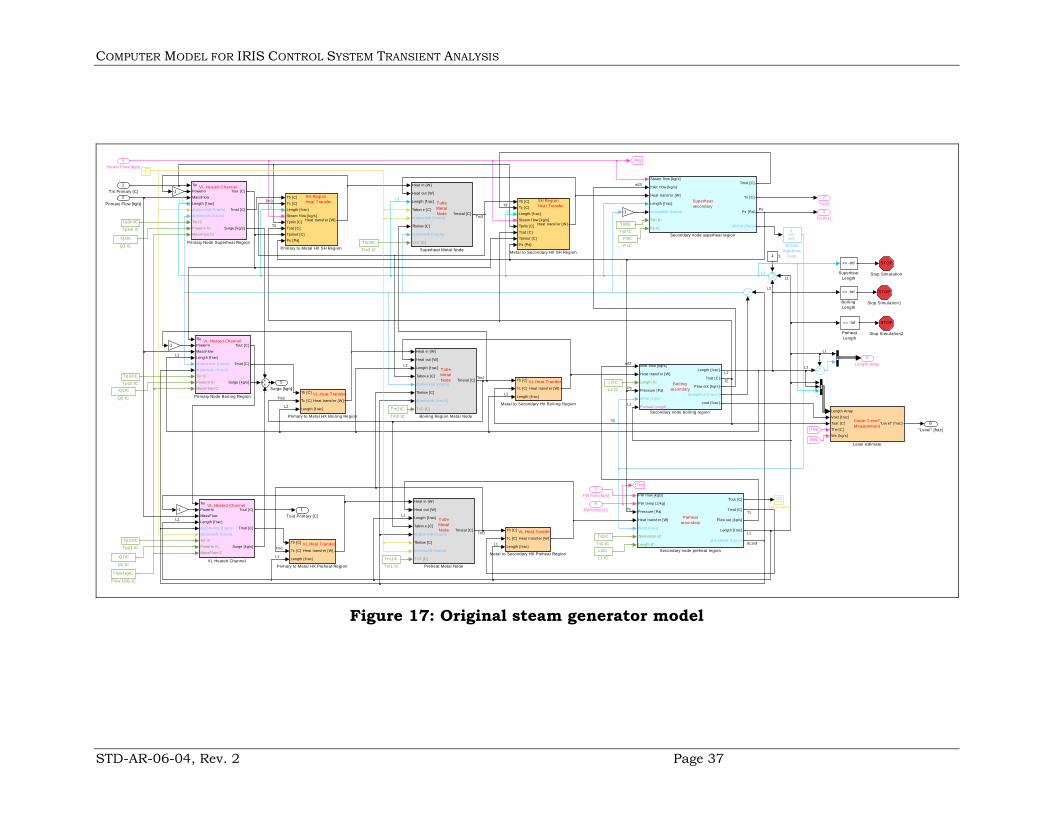
4.2.2.2.1.1 ORIGINAL MODEL
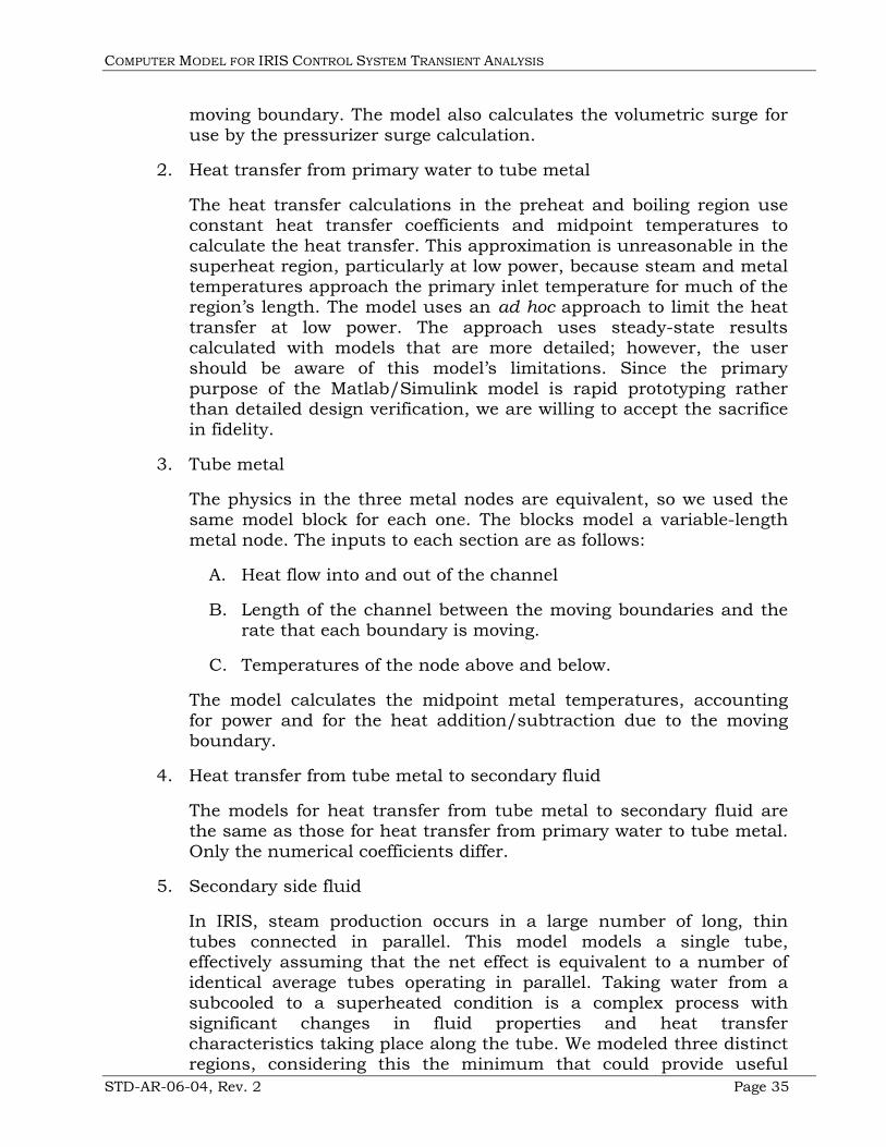
Figure 17 shows the original steam generator model. The model treats the secondary side of the steam generator as three regions with moving boundaries between regions. The regions, from inlet to outlet represent the preheat, boiling, and superheat regions. The model consists of fifteen major blocks arranged in three rows and five columns. From bottom to top, the rows represent the three regions just listed. From left to right, the columns are as follows:
1. Primary side water flow
The physics in the three primary nodes are equivalent, so we used the same model block for each one. The blocks model a variable-length heated channel. The inputs to each Section are as follows:
A. Mass flow and temperature into the channel
B. Power added to the fluid (normally negative)
C. Length of the channel between the moving boundaries and the rate that each boundary is moving.
The model calculates the midpoint and output temperatures, accounting for power and for the heat addition/subtraction due to the
COMPUTER MODEL FOR IRIS CONTROL SYSTEM TRANSIENT ANALYSIS
STD-AR-06-04, Rev. 2 Page 35
moving boundary. The model also calculates the volumetric surge for use by the pressurizer surge calculation.
2. Heat transfer from primary water to tube metal
The heat transfer calculations in the preheat and boiling region use constant heat transfer coefficients and midpoint temperatures to calculate the heat transfer. This approximation is unreasonable in the superheat region, particularly at low power, because steam and metal temperatures approach the primary inlet temperature for much of the region’s length. The model uses an ad hoc approach to limit the heat transfer at low power. The approach uses steady-state results calculated with models that are more detailed; however, the user should be aware of this model’s limitations. Since the primary purpose of the Matlab/Simulink model is rapid prototyping rather than detailed design verification, we are willing to accept the sacrifice in fidelity.
3. Tube metal
The physics in the three metal nodes are equivalent, so we used the same model block for each one. The blocks model a variable-length metal node. The inputs to each section are as follows:
A. Heat flow into and out of the channel
B. Length of the channel between the moving boundaries and the rate that each boundary is moving.
C. Temperatures of the node above and below.
The model calculates the midpoint metal temperatures, accounting for power and for the heat addition/subtraction due to the moving boundary.
4. Heat transfer from tube metal to secondary fluid
The models for heat transfer from tube metal to secondary fluid are the same as those for heat transfer from primary water to tube metal. Only the numerical coefficients differ.
5. Secondary side fluid
In IRIS, steam production occurs in a large number of long, thin tubes connected in parallel. This model models a single tube, effectively assuming that the net effect is equivalent to a number of identical average tubes operating in parallel. Taking water from a subcooled to a superheated condition is a complex process with significant changes in fluid properties and heat transfer characteristics taking place along the tube. We modeled three distinct regions, considering this the minimum that could provide useful
COMPUTER MODEL FOR IRIS CONTROL SYSTEM TRANSIENT ANALYSIS
STD-AR-06-04, Rev. 2 Page 36
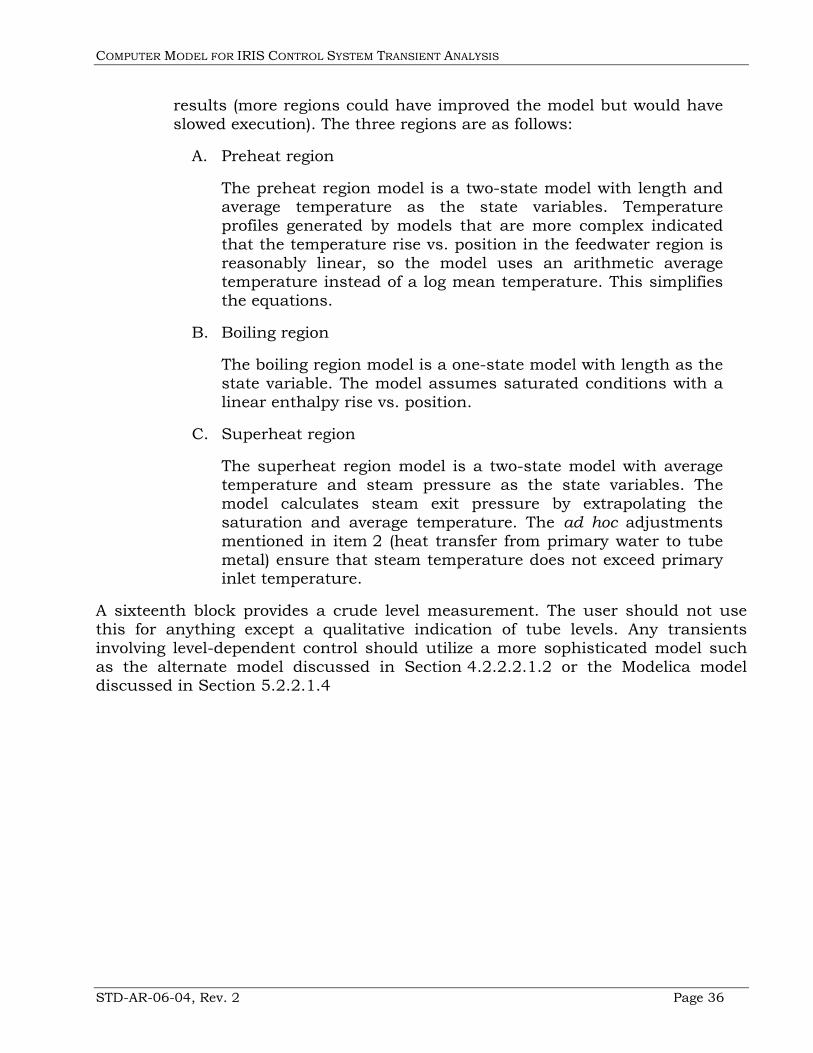
results (more regions could have improved the model but would have slowed execution). The three regions are as follows:
A. Preheat region
The preheat region model is a two-state model with length and average temperature as the state variables. Temperature profiles generated by models that are more complex indicated that the temperature rise vs. position in the feedwater region is reasonably linear, so the model uses an arithmetic average temperature instead of a log mean temperature. This simplifies the equations.
B. Boiling region
The boiling region model is a one-state model with length as the state variable. The model assumes saturated conditions with a linear enthalpy rise vs. position.
C. Superheat region
The superheat region model is a two-state model with average temperature and steam pressure as the state variables. The model calculates steam exit pressure by extrapolating the saturation and average temperature. The ad hoc adjustments mentioned in item 2 (heat transfer from primary water to tube metal) ensure that steam temperature does not exceed primary inlet temperature.
A sixteenth block provides a crude level measurement. The user should not use this for anything except a qualitative indication of tube levels. Any transients involving level-dependent control should utilize a more sophisticated model such as the alternate model discussed in Section 4.2.2.2.1.2 or the Modelica model discussed in Section 5.2.2.1.4
COMPUTER MODEL FOR IRIS CONTROL SYSTEM TRANSIENT ANALYSIS
STD-AR-06-04, Rev. 2 Page 37
6"Level" [frac]
5Surge [kg/s]
4Length Array
3Ps [Pa]
2Ts [c]
1Tout Primary [C]
Tin
PowerInMassFlowLength [f rac]dLabov e/dt [f rac/s]dLbelow/dt [f rac/s]
Tin ICPowerIn ICMassFlow IC
Tout [C]
Tmid [C]
Surge [kg/s]
VL Heated Channel
VL Heated Channel
Ts3IC
Ts3 IC
Ts1IC
Ts1 IC
Tp3inIC
Tp3in IC
Tp32IC
Tp32 IC
Tp21IC
Tp21 IC
Tm3IC
Tm3 IC
Tm2IC
Tm2 IC
Tm1IC
Tm1 IC
Terminator
Heat in [W]
Heat out [W]
Length [f rac]
Tabov e [C]
dLabov e/dt [f rac/s]
Tbelow [C]
dLbelow/dt [f rac/s]
T IC [C]
Tmetal [C]
TubeMetalNode
Superheat Metal Node
<= -Inf
SuperheatLength
STOP
Stop Simulation2
STOP
Stop Simulation1
STOP
Stop Simulation
Steam f low [kg/s]
Inlet f low [kg/s]
Heat transf er [W]
Length [f rac]
dLength/dt [f rac/s]
Tsh IC
Ps IC
Tmid [C]
Ts [C]
Ps [Pa]
dPs/dt [Pa/s]
Superheatsecondary
Secondary node superheat region
FW f low [kg/s]
FW temp [J/kg]
Pressure [Pa]
Heat transf er [W]
dP/dt [Pa/s]
Tpreheater IC
Length IC
Tout [C]
Tmid [C]
Flow out [kg/s]
Length [f rac]
dLength/dt [f rac/s]
Preheatsecondary
Secondary node preheat region
Inlet f low [kg/s]
Heat transf er [W]
Length IC
Pressure [Pa]
dP/dt [Pa/s]
Preheat Length
Length [f rac]
Tsat [C]
Flow out [kg/s]
dLength/dt [f rac/s]
v oid [f rac]
Boil ingsecondary
Secondary node boiling region
-Q3IC
Q3 IC
-Q2IC
Q2 IC
-Q1IC
Q1 IC
Th [C]
Tc [C]Length [f rac]Steam f low [kg/s]Tpriin [C]
Tsat [C]Tpriout [C]Ps [Pa]
Heat transf er [W]
SH RegionHeat Transfer
Primary to Metal HX SH Region
Th [C]
Tc [C]
Length [f rac]
Heat transf er [W]
VL Heat Transfer
Primary to Metal HX Preheat Region
Th [C]
Tc [C]
Length [f rac]
Heat transf er [W]
VL Heat Transfer
Primary to Metal HX Boiling Region
TinPowerInMassFlow
Length [f rac]dLabov e/dt [f rac/s]dLbelow/dt [f rac/s]Tin IC
PowerIn ICMassFlow IC
Tout [C]
Tmid [C]
Surge [kg/s]
VL Heated Channel
Primary Node Superheat Region
TinPowerInMassFlowLength [f rac]
dLabov e/dt [f rac/s]dLbelow/dt [f rac/s]Tin ICPowerIn IC
MassFlow IC
Tout [C]
Tmid [C]
Surge [kg/s]
VL Heated Channel
Primary Node Boil ing Region
Heat in [W]
Heat out [W]
Length [f rac]
Tabov e [C]
dLabov e/dt [f rac/s]
Tbelow [C]
dLbelow/dt [f rac/s]
T IC [C]
Tmetal [C]
TubeMetalNode
Preheat Metal Node
<= -Inf
PreheatLength
PsIC
P IC
Th [C]Tc [C]Length [f rac]
Steam f low [kg/s]Tpriin [C]Tsat [C]Tpriout [C]
Ps [Pa]
Heat transf er [W]
SH RegionHeat Transfer
Metal to Secondary HX SH Region
Th [C]
Tc [C]
Length [f rac]
Heat transf er [W]
VL Heat Transfer
Metal to Secondary HX Preheat Region
Th [C]
Tc [C]
Length [f rac]
Heat transf er [W]
VL Heat Transfer
Metal to Secondary HX Boiling Region
Length ArrayVoid [f rac]Tsat [C]
Tf w [C]Ws [kg/s]
"Lev el" [f rac]Crude "Level"Measurement
Level estimate
L2IC
L2 IC
L1IC
L1 IC
[Tfw]
[Ws]
-1
-1
-1
-1
[Tfw]
[Ws]
Flow1sgIC
Flow 1SG IC
1
s+1Breaks
AlgebraicLoop
Heat in [W]
Heat out [W]
Length [f rac]
Tabov e [C]
dLabov e/dt [f rac/s]
Tbelow [C]
dLbelow/dt [f rac/s]
T IC [C]
Tmetal [C]
TubeMetalNode
Boil ing Region Metal Node
<= -Inf
BoilingLength
1 1
5Steam Flow [kg/s]
4FW temp [C]
3FW flow [kg/s]
2Primary Flow [kg/s]
1Tin Primary [C]
T3L3
L3
L3
L3
L3
w12
L2
L2
L2
L2
L2
L2
L2
T1
L1
L1
L1
L1
L1
L1
L1
L1
dL1/dtTm1
Tm1
Tm2
Tm2
Tm3
Tm3
w23
Ps
Ps
Ps
T2
T2
T2
Figure 17: Original steam generator model
COMPUTER MODEL FOR IRIS CONTROL SYSTEM TRANSIENT ANALYSIS
STD-AR-06-04, Rev. 2 Page 38
4.2.2.2.1.2 ALTERNATE MODEL
Dr. Thomas Wilson of Oak Ridge National Labs is developing a moving boundary model based on an earlier helical-coil steam generator model (Reference 11) developed for sodium-cooled reactors. Except for the primary fluid properties, the steam generator design matches the IRIS design quite closely. Dr. Wilson’s model is considerably more rigorous than the one illustrated in Figure 17, and will provide far superior results at low powers.
4.2.2.2.2 STEAM SYSTEM
Figure 16 showed two steam system components: the steam lines model and the steam dump (a.k.a. turbine bypass) model.
The steam lines model takes steam conditions (temperature and pressure) and flow (turbine + turbine bypass) out of the steam header to calculate the flow from the steam generators. It also takes the steam conditions at the steam generator exit and calculates the conditions at the main steam header.
The steam dump (a.k.a. turbine bypass) model is a valve model that converts a flow demand signal to a total turbine bypass flow.
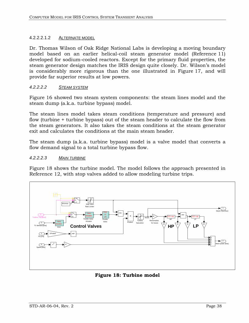
4.2.2.2.3 MAIN TURBINE
Figure 18 shows the turbine model. The model follows the approach presented in Reference 12, with stop valves added to allow modeling turbine trips.
Figure 18: Turbine model
Control Valves HP LP
2 Mech power [frac]
1 Steam flow [frac]
Turbine Saturation
Valve Actuator
Throttle Valve Actuator
Flow vs. Lift
Throttle Valve
Stop Valve Rate Limiter
-K- Renormalize
for losses Product min min
u 2
sqrt
GDS Lag LP GDS Lag
HP -K- -K- -K- -K-
-K-
1/Prated
Valve Actuator
EHC
Wsvmax
4 Speed [frac]
3 Turbine Trip [Bool]
2 TV demand [frac]
1 Ptv [Pa]
Wstun
COMPUTER MODEL FOR IRIS CONTROL SYSTEM TRANSIENT ANALYSIS
STD-AR-06-04, Rev. 2 Page 39
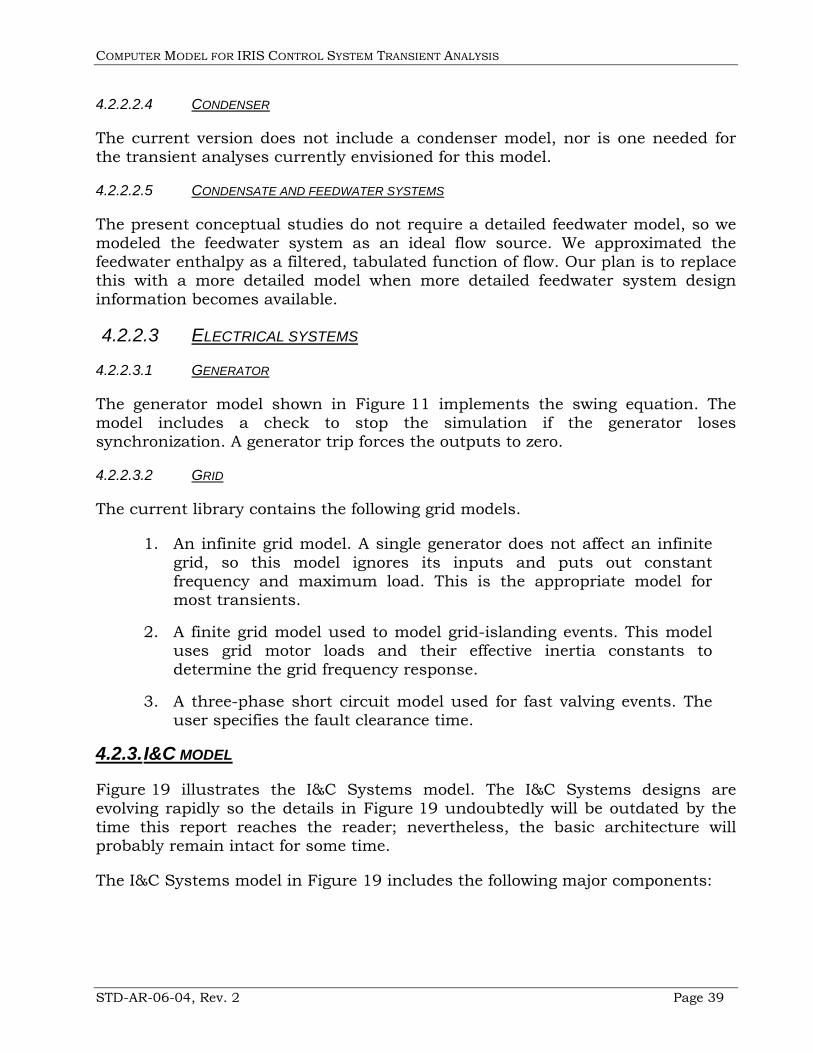
4.2.2.2.4 CONDENSER
The current version does not include a condenser model, nor is one needed for the transient analyses currently envisioned for this model.
4.2.2.2.5 CONDENSATE AND FEEDWATER SYSTEMS
The present conceptual studies do not require a detailed feedwater model, so we modeled the feedwater system as an ideal flow source. We approximated the feedwater enthalpy as a filtered, tabulated function of flow. Our plan is to replace this with a more detailed model when more detailed feedwater system design information becomes available.
4.2.2.3 ELECTRICAL SYSTEMS
4.2.2.3.1 GENERATOR
The generator model shown in Figure 11 implements the swing equation. The model includes a check to stop the simulation if the generator loses synchronization. A generator trip forces the outputs to zero.
4.2.2.3.2 GRID
The current library contains the following grid models.
1. An infinite grid model. A single generator does not affect an infinite grid, so this model ignores its inputs and puts out constant frequency and maximum load. This is the appropriate model for most transients.
2. A finite grid model used to model grid-islanding events. This model uses grid motor loads and their effective inertia constants to determine the grid frequency response.
3. A three-phase short circuit model used for fast valving events. The user specifies the fault clearance time.
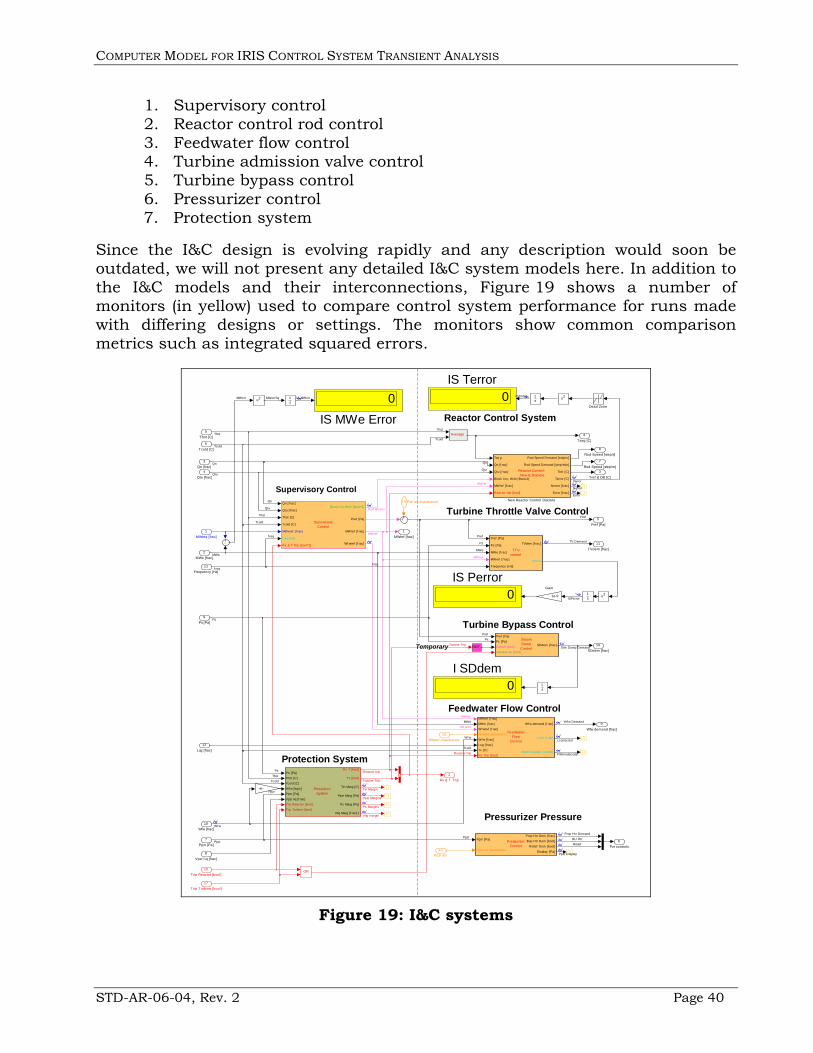
4.2.3. I&C MODEL
Figure 19 illustrates the I&C Systems model. The I&C Systems designs are evolving rapidly so the details in Figure 19 undoubtedly will be outdated by the time this report reaches the reader; nevertheless, the basic architecture will probably remain intact for some time.
The I&C Systems model in Figure 19 includes the following major components:
COMPUTER MODEL FOR IRIS CONTROL SYSTEM TRANSIENT ANALYSIS
STD-AR-06-04, Rev. 2 Page 40
1. Supervisory control 2. Reactor control rod control 3. Feedwater flow control 4. Turbine admission valve control 5. Turbine bypass control 6. Pressurizer control 7. Protection system
Since the I&C design is evolving rapidly and any description would soon be outdated, we will not present any detailed I&C system models here. In addition to the I&C models and their interconnections, Figure 19 shows a number of monitors (in yellow) used to compare control system performance for runs made with differing designs or settings. The monitors show common comparison metrics such as integrated squared errors.
Reactor Control System
Turbine Throttle Valve Control
Feedwater Flow Control
||||||||||||||||||||||||||||||||||||||||||||||||||||||||||||||||||||||||||||||||||||||||||||||||||||||||||||||||||||
Supervisory Control
Turbine Bypass Control
Pressurizer Pressure
Protection System
Temporary
11TVdem [frac]
10SDdem [frac]
9Wfw demand [frac]
8Rod Speed [step/s]
7Rod Speed [step/m]
6Pzr controls
5Pref [Pa]
4Tavg [C]
3Tref & DB [C]
2Rx & T Trip
1MWref [frac]
-K-
Pref [Pa]
Ps [Pa]
MWe [f rac]
MWref [f rac]
Frequency [Hz]
TVdem [f rac]
Perror
TTVcontrol
Qn [f rac]
Qtu [f rac]
Thot [C]
Tcold [C]
MWeref [f rac]
f req [Hz]
Rx & T Trip [bool*2]
Block Ins;With [Bool*2]
Pref [Pa]
MWref [f rac]
Wf wref [f rac]
SupervisoryControl
Pref [Pa]Ps [Pa]
DeltaP [bool]
Initialize on [bool]
SDdem [f rac]
SteamDump
Control
Ps [Pa]Thot [C]
Tcold [C]
Wf w [kg/s]
Ppzr [Pa]
Vpzr liq [f rac]Trip Reactor [bool]
Trip Turbine [bool]
Rx T [bool]
TT [bool]
Tin Marg [C]
Ppzr Marg [Pa]
Ps Marg [Pa]
Vliq Marg [f rac]1
ProtectionSystem
Ppzr [Pa]
Ppzr ref disturbance
Prop Htr Dem [f rac]
Bup Htr Dem [bool]
Relief Dem [bool]
Display [Pa]
PressurizerControl
Tav g
Qn [f rac]
Qtu [f rac]
Block Ins; With [Boolx2]
MWref [f rac]
Reactor trip [bool]
Rod Speed Demand [step/s]
Rod Speed Demand [step/min]
Tref [C]
Terror [C]
Nerror [f rac]
Error [f rac]
Reactor Control: New & Discrete
New Reactor Control Discrete
u2
u2
u2
OR
NOT
1s
1s
1s
1s0
IS Terror
0IS Perror
0
IS MWe Error
0I SDdem
1e-9
Gain
MWref [f rac]MWe [f rac]
Wf wref [f rac]
Wf wref disturbance
Wf w [f rac]
Lsg [f rac]Tc [C]
Rx Trip [bool]
Wf w demand [f rac]
Lcorr [f rac]
Mode Display [coded]
FeedwaterFlow
Control
Dead Zone
Average
17Trip Turbine [bool]
16Trip Reactor [bool]
15Wfwref disturbance
14 Psh ref disturbance
13Ppzr ref
12Lsg [frac]
11Frequency [Hz]
10Wfw [frac]
9Ps [Pa]
8Vpzr l iq [frac]
7Ppzr [Pa]
6Tcold [C]
5Thot [C]
4Qtu [frac]
3Qn [frac]
2MWe [frac]
1MWreq [frac]
Pref
Pref
Pref
Ps
Ps
Ps
Ps
Thot
Thot
Thot
Thot
Tcold
Tcold
Tcold
Tcold
Tcold
Qn
Qn
Qn
Wf wref
MWe
MWeMWe
TV Demand
f req
f reqf req
MWref
MWref
MWref
MWref
Wf w Demand
Wf w
Wf w
Stm Dump Demand
Ppzr
PpzrPpzr
Prop Htr Demand
BU HtrRelief
Qtu
Qtu
Qtu
Rod Blocks
Terror
ISTerror
Nerror
Error
Ppzr Display
Tin Margin
Ppzr Margins
Ps Margins
Reactor trip
Reactor trip
Vliq margin
Turbine Trip
Turbine Trip
FWmodecode
Lcorrected
ISPerror
MWerrSq IS MWerrMWerr
Figure 19: I&C systems
COMPUTER MODEL FOR IRIS CONTROL SYSTEM TRANSIENT ANALYSIS
STD-AR-06-04, Rev. 2 Page 41
5. THE MODELICA MODEL
5.1. MODEL OVERVIEW
5.1.1. MODEL PURPOSE
Our Modelica IRIS model sits at the center of the project’s model hierarchy. While the Matlab/Simulink model focus on rapid prototyping led to extensive simplification, the Modelica model incorporates greater modeling detail. We plan to use the Matlab/Simulink model for rapid prototyping and initial design evaluation and then use the Modelica model for more detailed assessments.
We envision using the Modelica model to confirm control system performance, to establish operating strategies, to verify that there is adequate margin to component and protection limits for all normal operating events (and selected upsets), and to establish preliminary control system set points. When we begin constructing an IRIS plant and select the appropriate I&C platform, we will probably move to another modeling environment that gives the modeler the control needed to do the very specific modeling needed to confirm proper I&C system software implementation.
5.1.2. MODELING ENVIRONMENT
The Modelica language allows convenient, component-oriented modeling of complex physical systems. The non-profit Modelica Association provides the Modelica language, Modelica libraries, and Modelica simulation tools without cost, but one needs a compatible development environment to use these. Westinghouse uses Dymola (Dynamic Modeling Laboratory, see Reference 13), a complete tool for modeling and simulation of integrated and complex systems in Modelica. Dymola provides means to develop Modelica models graphically, textually, or in hybrid combinations of the two.
Modelica is an object-oriented language whose inheritance features allow the user to modify the model by substituting one version of a class for another. For example, one can substitute one set of water properties (“steam tables”) for another. Another example, which we used in our model, is to allow the user to substitute one sensor dynamics model for another.
Modelica works with equations rather than assignment statements. The Dymola environment provides computer algebra tools to manipulate the equations into a form that allows convenient numerical solution. The manipulation occurs “behind the scenes.” This relieves the developer of much of the burden normally associated with transforming and ordering physical equations into a form amenable to numerical integration. Unfortunately, this eliminates most of the
COMPUTER MODEL FOR IRIS CONTROL SYSTEM TRANSIENT ANALYSIS
STD-AR-06-04, Rev. 2 Page 42
developer’s control as well. We noticed that ensuring that a model initializes properly is particularly troublesome. The numerous nonlinear elements found in most control systems often lead to equations with several mathematically correct solutions only one of which is physically reasonable. The Dymola/Modelica combination does not always find the desired solution. Aggravating this problem, the Dymola debugging facilities do not provide much useful assistance. The developer needs to address these on a case-by-case basis as problems arise. Despite these difficulties, the Dymola/Modelica combination gives the user the ability to quickly develop different versions of the same model that vary in detail, allowing the user to reach a reasonable balance between execution speed and model detail.
5.2. THE MODEL
The first IRIS model suitable for control studies was the Modelica model developed at POLIMI (Reference 3). We examined this model in 2004 and concluded that we needed a faster model. Francisco Schiavo simplified the POLIMI model, increasing its speed by an order of magnitude. We illustrate the types of simplifications made with the following two examples:
1. The reactor coolant flow inside the IRIS vessel has a number of small bypass flow paths. The original Modelica model included these (Figure 20, left), but the resulting equations translated, initialized, and executed quite slowly. Although the parasitic flows are small, the model still had to balance mass and energy flows at each node while maintaining the full nonlinearity of the chosen steam table water properties. Simplifying the flow paths (Figure 20, right) improved code performance considerably with little sacrifice in fidelity. The user could revert to the left-hand model in Figure 20 if necessary.
2. In several cases, we found it convenient to develop alternate versions of the same functions. For example, we defined the primary and secondary fluids as replaceable media. This let us develop one version that used the IF97 steam table routines, while another version uses simple curve fits. There are some effects, such as the expansion temperature drop associated with liquid water flowing through a small pressure drop, that are simply too small to justify the computational burden required to account for them. The assumption that the reactor coolant enthalpy is independent of pressure is reasonable for most normal operating transients. Once again, the user always has the option of selecting the more detailed – but slower – model.

COMPUTER MODEL FOR IRIS CONTROL SYSTEM TRANSIENT ANALYSIS
STD-AR-06-04, Rev. 2 Page 43
The result of earlier simplifications was the model used for the analyses reported in Reference 2. We continue to refine the model, making use of knowledge gained over the past two years.
Figure 20: Reactor coolant flow path models
5.2.1. HIGH-LEVEL STRUCTURE
5.2.1.1 MODEL COMPONENTS
Figure 21: Modelica root-level model
Figure 21 shows the root-level view of the Modelica model. The model has the following major blocks:
COMPUTER MODEL FOR IRIS CONTROL SYSTEM TRANSIENT ANALYSIS
STD-AR-06-04, Rev. 2 Page 44
1. Nuclear steam supply system (NSSS)
The NSSS block includes models for the major components within the IRIS, such as the core, reactor coolant pumps, steam generators, and pressurizer. The NSSS receives feedwater from and sends steam to the TGFWS via the bottom and top connections on the left side of the NSSS icon. The NSSS supplies sensor signals to the sensor bus via the square blue port, and receives actuator command signals via the square red port. Section 5.2.2.1 describes the NSSS model in more detail.
2. Turbine/Generator/Feedwater Systems (TGFWS)
The TGFWS block includes models for the following items:
A. Main steam system, including turbine bypass valves
B. Main turbine
C. Generator and generator breaker
D. External electrical grid
E. Feedwater source
The TGFWS block interfaces to the NSSS block via the feedwater and steam interfaces described in item 1. Section 5.2.2.1.4 describes the TGFWS model in more detail.
3. Control systems (CS)
The CS block contains or will contain models for the major plant I&C systems, including the safety-related protection system and the non-safety-related control systems. It interfaces with the measurement1 bus (green, providing inputs), actuator bus (red, receiving outputs), and supervisory bus (black, with bidirectional communication). Section 5.2.3.1 describes the CS model in more detail.
4. Supervisory signals (SS)
The original model developers intended to have the SS class represent the supervisory control system, but we moved that function to the CS class so that the SS class’s scope would be limited to external interfaces. The SS class now provides human
1 In earlier versions of the model, the CS module interfaced directly with the sensor bus. This is
why the CS icon has a blue square rather than a green square at the interface port. The color has no functional significance.

COMPUTER MODEL FOR IRIS CONTROL SYSTEM TRANSIENT ANALYSIS
STD-AR-06-04, Rev. 2 Page 45
interface signals (e.g., power change requests) and external interface signals (e.g., remote dispatching). These signals define the transient that the user wishes to analyze. The SS block has a bi-directional interface with the supervisory bus. Section 5.2.3.2 describes the SS model in more detail.
5. Sensor dynamics
The NSSS and TGFWS place sensor signals on the blue sensor bus. These pure signals represent the actual process variable without distortion, noise, or delay. The sensor dynamics block models the imperfections of real sensors. Section 5.2.3.3 describes the sensor dynamics model(s) in more detail.
6. Signal buses
There are four expandable buses defined in the model, as follows:
A. Sensor bus (blue), containing signals that represent the actual process variable without distortion, noise, or delay.
B. Measurement bus (green), containing signals that represent measured process variables with associated sensor distortion, noise, and delay.
C. Actuator bus (red), containing demand signals from the control and protection systems to the actuated components. Generally, the model structure includes actuator dynamics as part of the actuated component in the NSSS or TGFWS blocks.
D. Supervisory bus (black), containing operator or dispatcher signals define the transient to be analyzed and associated feedbacks from the control systems.
There is no user-generated code for the buses per se; instead, the interfacing blocks define the bus signals. There is no requirement that a signal placed on a bus have an associated destination.
5.2.1.2 USER INTERFACE
The user must provide several data to control model execution. The major files are as follows:
1. NSSSData
The NSSSData file contains the data needed to define the power-independent parameters for the NSSS model. Examples include dimensional data, heat transfer data, and hydraulic data. This file includes data that describe the nominal full-power operating
COMPUTER MODEL FOR IRIS CONTROL SYSTEM TRANSIENT ANALYSIS
STD-AR-06-04, Rev. 2 Page 46
conditions. It also contains operating curves for some components such as the reactor coolant pump head vs. flow curves. The general criterion for including data in this file instead of initNSSSData is that the information in NSSSData will rarely change from one transient analysis to the next.
2. initNSSSData
The initNSSSData file contains data that describes the initial conditions for a particular analysis. In general, the data in this file vary as a function of initial operating power, although they might also vary with plant configuration. Typical information includes thermodynamic data (temperatures, pressures, enthalpies, etc), and initial reactor power.
3. TGFWSData
The TGFWSData file contains the data needed to define the power-independent parameters for the TGFWS model. Examples include characteristic times, thermodynamic data, and hydraulic data. This file includes data that describe the nominal full-power operating conditions. The general criterion for including data in this file instead of initTGFWSData is that the information in TGFWSData will rarely change from one transient analysis to the next.
4. initTGFWSData
The initTGFWSData file contains data that describes the initial conditions for a particular analysis. In general, the data in this file vary as a function of initial operating power, although they might also vary with plant configuration. Typically, this information involves thermodynamic data (temperatures, pressures, enthalpies, etc).
5. SensorTaus
Section 5.2.3.3 describes several sensor dynamics models that the user may select. The SensorTaus file includes the data needed to describe the performance of specific sensor types. The file structure may change for different sensor model selections.
6. CSData
Section 5.2.3.1 describes the control and protection system model. The CSData file includes the data needed to describe the configuration and settings for specific control system models. The file structure may change for different control system model selections.
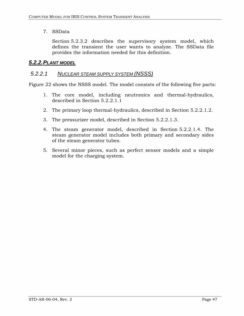
COMPUTER MODEL FOR IRIS CONTROL SYSTEM TRANSIENT ANALYSIS
STD-AR-06-04, Rev. 2 Page 47
7. SSData
Section 5.2.3.2 describes the supervisory system model, which defines the transient the user wants to analyze. The SSData file provides the information needed for this definition.
5.2.2. PLANT MODEL
5.2.2.1 NUCLEAR STEAM SUPPLY SYSTEM (NSSS)
Figure 22 shows the NSSS model. The model consists of the following five parts:
1. The core model, including neutronics and thermal-hydraulics, described in Section 5.2.2.1.1
2. The primary loop thermal-hydraulics, described in Section 5.2.2.1.2.
3. The pressurizer model, described in Section 5.2.2.1.3.
4. The steam generator model, described in Section 5.2.2.1.4. The steam generator model includes both primary and secondary sides of the steam generator tubes.
5. Several minor pieces, such as perfect sensor models and a simple model for the charging system.

COMPUTER MODEL FOR IRIS CONTROL SYSTEM TRANSIENT ANALYSIS
STD-AR-06-04, Rev. 2 Page 48
Figure 22: NSSS model
5.2.2.1.1 CORE
The core icon appears in red near the bottom of Figure 22. Figure 23 shows the following four major internal components:
1. A ThermoPower2 ThermoPower.Water.Flow1D class, modified to put out moderator temperature and density for the kinetics class. Moderator flow is upwards in Figure 23.
2. A FuelRods class that models the fuel temperature. The model divides the fuel into five radial zones (three within the fuel pellet, one for the gap, and one for the cladding) and a user-specified number of axial zones. The present model uses a pre-specified axial power distribution that may be taken as uniform for the present studies. The model defines the fuel properties, cladding properties, and gap heat transfer correlations as replaceable functions so that the user
2 The ThermoPower library is an open Modelica library for the dynamic modeling of thermal
power plants. The library has been developed to analyze the dynamic behavior of plants, with the purpose of studying control system strategies and architectures. Reference 13 provides detailed information.
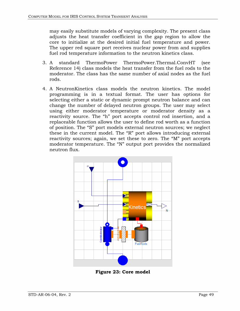
COMPUTER MODEL FOR IRIS CONTROL SYSTEM TRANSIENT ANALYSIS
STD-AR-06-04, Rev. 2 Page 49
may easily substitute models of varying complexity. The present class adjusts the heat transfer coefficient in the gap region to allow the core to initialize at the desired initial fuel temperature and power. The upper red square port receives nuclear power from and supplies fuel rod temperature information to the neutron kinetics class.
3. A standard ThermoPower ThermoPower.Thermal.ConvHT (see Reference 14) class models the heat transfer from the fuel rods to the moderator. The class has the same number of axial nodes as the fuel rods.
4. A NeutronKinetics class models the neutron kinetics. The model programming is in a textual format. The user has options for selecting either a static or dynamic prompt neutron balance and can change the number of delayed neutron groups. The user may select using either moderator temperature or moderator density as a reactivity source. The “h” port accepts control rod insertion, and a replaceable function allows the user to define rod worth as a function of position. The “S” port models external neutron sources; we neglect these in the current model. The “R” port allows introducing external reactivity sources; again, we set these to zero. The “M” port accepts moderator temperature. The “N” output port provides the normalized neutron flux.
Figure 23: Core model
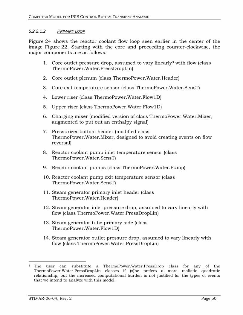
COMPUTER MODEL FOR IRIS CONTROL SYSTEM TRANSIENT ANALYSIS
STD-AR-06-04, Rev. 2 Page 50
5.2.2.1.2 PRIMARY LOOP
Figure 24 shows the reactor coolant flow loop seen earlier in the center of the image Figure 22. Starting with the core and proceeding counter-clockwise, the major components are as follows:
1. Core outlet pressure drop, assumed to vary linearly3 with flow (class ThermoPower.Water.PressDropLin)
2. Core outlet plenum (class ThermoPower.Water.Header)
3. Core exit temperature sensor (class ThermoPower.Water.SensT)
4. Lower riser (class ThermoPower.Water.Flow1D)
5. Upper riser (class ThermoPower.Water.Flow1D)
6. Charging mixer (modified version of class ThermoPower.Water.Mixer, augmented to put out an enthalpy signal)
7. Pressurizer bottom header (modified class ThermoPower.Water.Mixer, designed to avoid creating events on flow reversal)
8. Reactor coolant pump inlet temperature sensor (class ThermoPower.Water.SensT)
9. Reactor coolant pumps (class ThermoPower.Water.Pump)
10. Reactor coolant pump exit temperature sensor (class ThermoPower.Water.SensT)
11. Steam generator primary inlet header (class ThermoPower.Water.Header)
12. Steam generator inlet pressure drop, assumed to vary linearly with flow (class ThermoPower.Water.PressDropLin)
13. Steam generator tube primary side (class ThermoPower.Water.Flow1D)
14. Steam generator outlet pressure drop, assumed to vary linearly with flow (class ThermoPower.Water.PressDropLin)
3 The user can substitute a ThermoPower.Water.PressDrop class for any of the
ThermoPower.Water.PressDropLin classes if (s)he prefers a more realistic quadratic relationship, but the increased computational burden is not justified for the types of events that we intend to analyze with this model.
COMPUTER MODEL FOR IRIS CONTROL SYSTEM TRANSIENT ANALYSIS
STD-AR-06-04, Rev. 2 Page 51
15. Steam generator primary outlet header (class ThermoPower.Water.Header)
16. Steam generator exit temperature sensor (class ThermoPower.Water.SensT)
17. Lower downcomer (class ThermoPower.Water.Flow1D)
18. Lower plenum (class ThermoPower.Water.Header)
19. Core inlet temperature sensor (class ThermoPower.Water.SensT)
20. Core inlet pressure drop, assumed to vary linearly with flow (class ThermoPower.Water.PressDropLin)
Each of these, including the core, allows replacing the fluid medium model. This allows the user to specify either a simplified medium model to increase computational speed or a more detailed model to improve fidelity. The types of events that we intend to analyze with this model probably do not require highly detailed fluid models such as the IF97 steam table models presently used as the default.
Each temperature sensor has an associated block to convert from SI temperature units (Kelvin) to IRIS project units (Celsius).
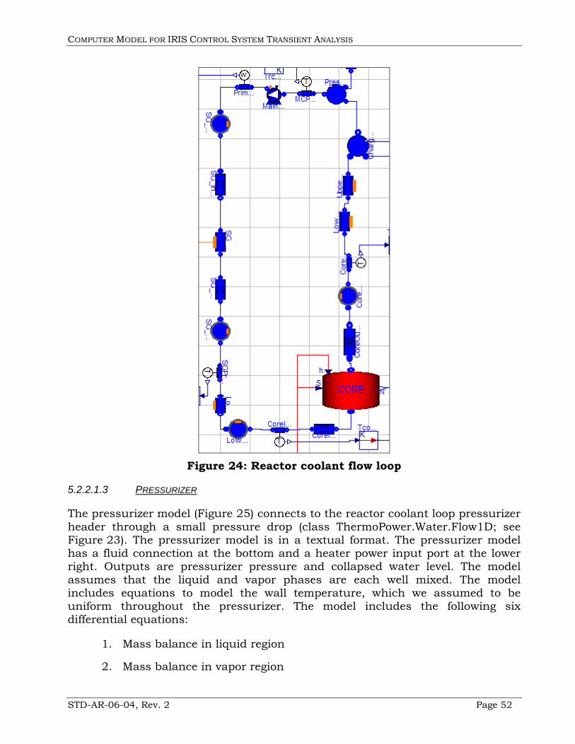
COMPUTER MODEL FOR IRIS CONTROL SYSTEM TRANSIENT ANALYSIS
STD-AR-06-04, Rev. 2 Page 52
Figure 24: Reactor coolant flow loop
5.2.2.1.3 PRESSURIZER
The pressurizer model (Figure 25) connects to the reactor coolant loop pressurizer header through a small pressure drop (class ThermoPower.Water.Flow1D; see Figure 23). The pressurizer model is in a textual format. The pressurizer model has a fluid connection at the bottom and a heater power input port at the lower right. Outputs are pressurizer pressure and collapsed water level. The model assumes that the liquid and vapor phases are each well mixed. The model includes equations to model the wall temperature, which we assumed to be uniform throughout the pressurizer. The model includes the following six differential equations:
1. Mass balance in liquid region
2. Mass balance in vapor region

COMPUTER MODEL FOR IRIS CONTROL SYSTEM TRANSIENT ANALYSIS
STD-AR-06-04, Rev. 2 Page 53
3. Energy balance in liquid region
4. Energy balance in vapor region
5. Energy balance in metal wall
6. Pressurizer heaters thermal time constant
The model includes the following mass and energy transfers:
1. Heat transfer from heaters to liquid
2. Mass and energy flow through the lower fluid connection
3. Bulk liquid evaporation (when not subcooled)
4. Bulk vapor condensation (when not superheated)
5. Vapor condensation on metal wall
6. Direct heat transfer from liquid to vapor (due to temperature difference)
Figure 25: Pressurizer icon
5.2.2.1.4 STEAM GENERATOR
The steam generator model is spread across several classes and, hence, across several graphical views. Figure 26 shows the portion of Figure 22 that models fluid flow and heat transfer to the helical coil metal. In the center right is the steam generator tube primary side model (class ThermoPower.Water.Flow1D) discussed in Section 5.2.2.1.2. The orange distributed heat terminal (class ThermoPower.Thermal.DHT) provides a multi-node temperature and heat transfer interface between the primary fluid and the tube wall convective heat transfer model (class ThermoPower.Thermal.ConvHT) shown in the center of Figure 26. This, in turn, interfaces with another distributed heat terminal (class ThermoPower.Thermal.DHT) on the helical coil model shown at the right.
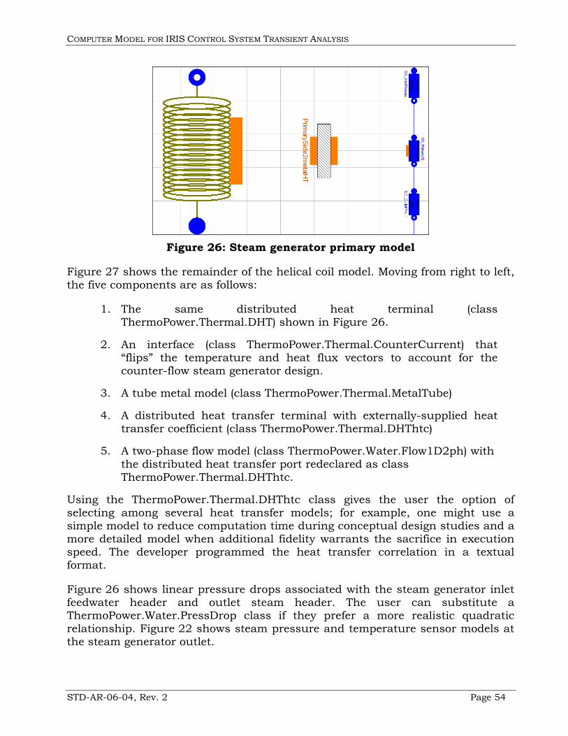
COMPUTER MODEL FOR IRIS CONTROL SYSTEM TRANSIENT ANALYSIS
STD-AR-06-04, Rev. 2 Page 54
Figure 26: Steam generator primary model
Figure 27 shows the remainder of the helical coil model. Moving from right to left, the five components are as follows:
1. The same distributed heat terminal (class ThermoPower.Thermal.DHT) shown in Figure 26.
2. An interface (class ThermoPower.Thermal.CounterCurrent) that “flips” the temperature and heat flux vectors to account for the counter-flow steam generator design.
3. A tube metal model (class ThermoPower.Thermal.MetalTube)
4. A distributed heat transfer terminal with externally-supplied heat transfer coefficient (class ThermoPower.Thermal.DHThtc)
5. A two-phase flow model (class ThermoPower.Water.Flow1D2ph) with the distributed heat transfer port redeclared as class ThermoPower.Thermal.DHThtc.
Using the ThermoPower.Thermal.DHThtc class gives the user the option of selecting among several heat transfer models; for example, one might use a simple model to reduce computation time during conceptual design studies and a more detailed model when additional fidelity warrants the sacrifice in execution speed. The developer programmed the heat transfer correlation in a textual format.
Figure 26 shows linear pressure drops associated with the steam generator inlet feedwater header and outlet steam header. The user can substitute a ThermoPower.Water.PressDrop class if they prefer a more realistic quadratic relationship. Figure 22 shows steam pressure and temperature sensor models at the steam generator outlet.

COMPUTER MODEL FOR IRIS CONTROL SYSTEM TRANSIENT ANALYSIS
STD-AR-06-04, Rev. 2 Page 55
Figure 27: Steam generator model, excluding primary
5.2.2.1.5 CHARGING SYSTEM
Although we do not anticipate using this Modelica model to analyze events that involve charging flow variations, we included provisions for adding a charging flow model later. Figure 22 shows a net charging flow source that provides fluid at the existing charging mixer enthalpy. At this time, we normally set the (net) charging flow equal to zero.
5.2.2.2 TURBINE/GENERATOR/FEEDWATER SYSTEMS (TGFWS)
Figure 28 shows the TGFWS model. The model receives steam at the upper right-hand fluid connection, and delivers feedwater at the lower fluid connection. The red and blue square ports receive actuator demands and deliver sensed process variable values, respectively. The major component groups are as follows:
1. Steam System, described in Section 5.2.2.2.1
2. Main turbine, described in Section 5.2.2.2.2
3. Condenser, described in Section 5.2.2.2.3
4. Condensate and feedwater systems, described in Section 5.2.2.2.6
4. Generator, described in Section 5.2.2.2.3
5. Electrical loads, described in Section 5.2.2.2.4
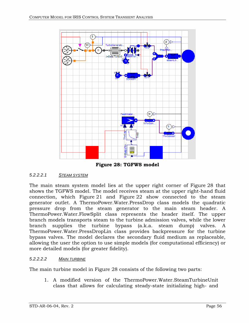
COMPUTER MODEL FOR IRIS CONTROL SYSTEM TRANSIENT ANALYSIS
STD-AR-06-04, Rev. 2 Page 56
Figure 28: TGFWS model
5.2.2.2.1 STEAM SYSTEM
The main steam system model lies at the upper right corner of Figure 28 that shows the TGFWS model. The model receives steam at the upper right-hand fluid connection, which Figure 21 and Figure 22 show connected to the steam generator outlet. A ThermoPower.Water.PressDrop class models the quadratic pressure drop from the steam generator to the main steam header. A ThermoPower.Water.FlowSplit class represents the header itself. The upper branch models transports steam to the turbine admission valves, while the lower branch supplies the turbine bypass (a.k.a. steam dump) valves. A ThermoPower.Water.PressDropLin class provides backpressure for the turbine bypass valves. The model declares the secondary fluid medium as replaceable, allowing the user the option to use simple models (for computational efficiency) or more detailed models (for greater fidelity).
5.2.2.2.2 MAIN TURBINE
The main turbine model in Figure 28 consists of the following two parts:
1. A modified version of the ThermoPower.Water.SteamTurbineUnit class that allows for calculating steady-state initializing high- and
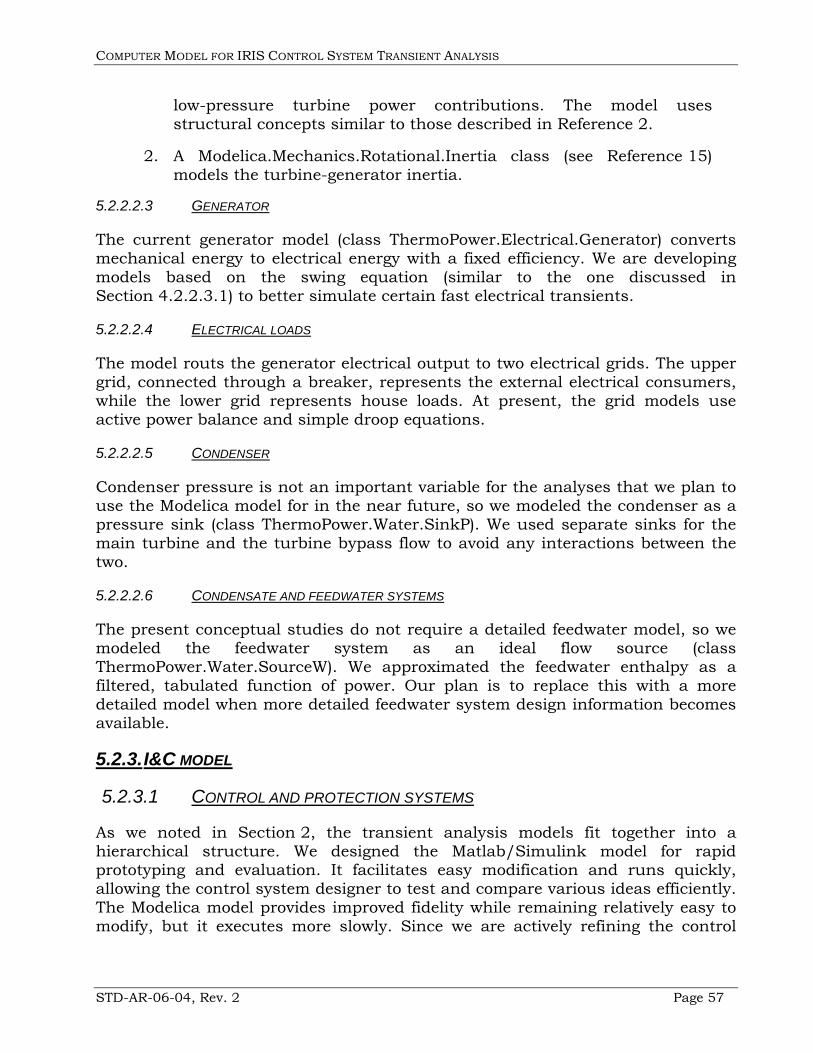
COMPUTER MODEL FOR IRIS CONTROL SYSTEM TRANSIENT ANALYSIS
STD-AR-06-04, Rev. 2 Page 57
low-pressure turbine power contributions. The model uses structural concepts similar to those described in Reference 2.
2. A Modelica.Mechanics.Rotational.Inertia class (see Reference 15) models the turbine-generator inertia.
5.2.2.2.3 GENERATOR
The current generator model (class ThermoPower.Electrical.Generator) converts mechanical energy to electrical energy with a fixed efficiency. We are developing models based on the swing equation (similar to the one discussed in Section 4.2.2.3.1) to better simulate certain fast electrical transients.
5.2.2.2.4 ELECTRICAL LOADS
The model routs the generator electrical output to two electrical grids. The upper grid, connected through a breaker, represents the external electrical consumers, while the lower grid represents house loads. At present, the grid models use active power balance and simple droop equations.
5.2.2.2.5 CONDENSER
Condenser pressure is not an important variable for the analyses that we plan to use the Modelica model for in the near future, so we modeled the condenser as a pressure sink (class ThermoPower.Water.SinkP). We used separate sinks for the main turbine and the turbine bypass flow to avoid any interactions between the two.
5.2.2.2.6 CONDENSATE AND FEEDWATER SYSTEMS
The present conceptual studies do not require a detailed feedwater model, so we modeled the feedwater system as an ideal flow source (class ThermoPower.Water.SourceW). We approximated the feedwater enthalpy as a filtered, tabulated function of power. Our plan is to replace this with a more detailed model when more detailed feedwater system design information becomes available.
5.2.3. I&C MODEL
5.2.3.1 CONTROL AND PROTECTION SYSTEMS
As we noted in Section 2, the transient analysis models fit together into a hierarchical structure. We designed the Matlab/Simulink model for rapid prototyping and evaluation. It facilitates easy modification and runs quickly, allowing the control system designer to test and compare various ideas efficiently. The Modelica model provides improved fidelity while remaining relatively easy to modify, but it executes more slowly. Since we are actively refining the control

COMPUTER MODEL FOR IRIS CONTROL SYSTEM TRANSIENT ANALYSIS
STD-AR-06-04, Rev. 2 Page 58
system designs, the I&C portion of the Modelica model naturally lags behind the Matlab/Simulink model.
There are two major variations of the present Modelica model. The first version is a conceptual design model focused on plant model development. It uses trivial4 I&C models so that I&C development issues do not impede plant modeling. The second is the I&C development version. This has the same plant models as the conceptual model, but it starts to add detailed control system models. We found that Modelica’s automated initialization presents problems with analog control models featuring significant nonlinearities. Working through these problems is taking time. Although we have not finished creating the initial control system models in the current Modelica model, we still have the 2004 models that we used for the analyses presented in Reference 2. Figure 29 shows the overall control system model structure used in 2004. It is cluttered, mainly because it does not make use of the bus structure that we use in the current model.
Figure 29: 2004 control systems model
Figure 30 shows the current control systems model structure at an early developmental stage. Starting with the conceptual design model, we began by replacing the turbine admission valve control and pressurizer heater control models with operating versions. We are replacing the remaining blocks in a similar manner. Note that we retained the modular control system structure seen in Figure 29, but it will utilize bus structures to reduce the external clutter. This should make the model easier to understand and maintain.
4 Since the conceptual model’s purpose is to develop the plant model, many of the associated
control system models take no closed-loop control action at all.
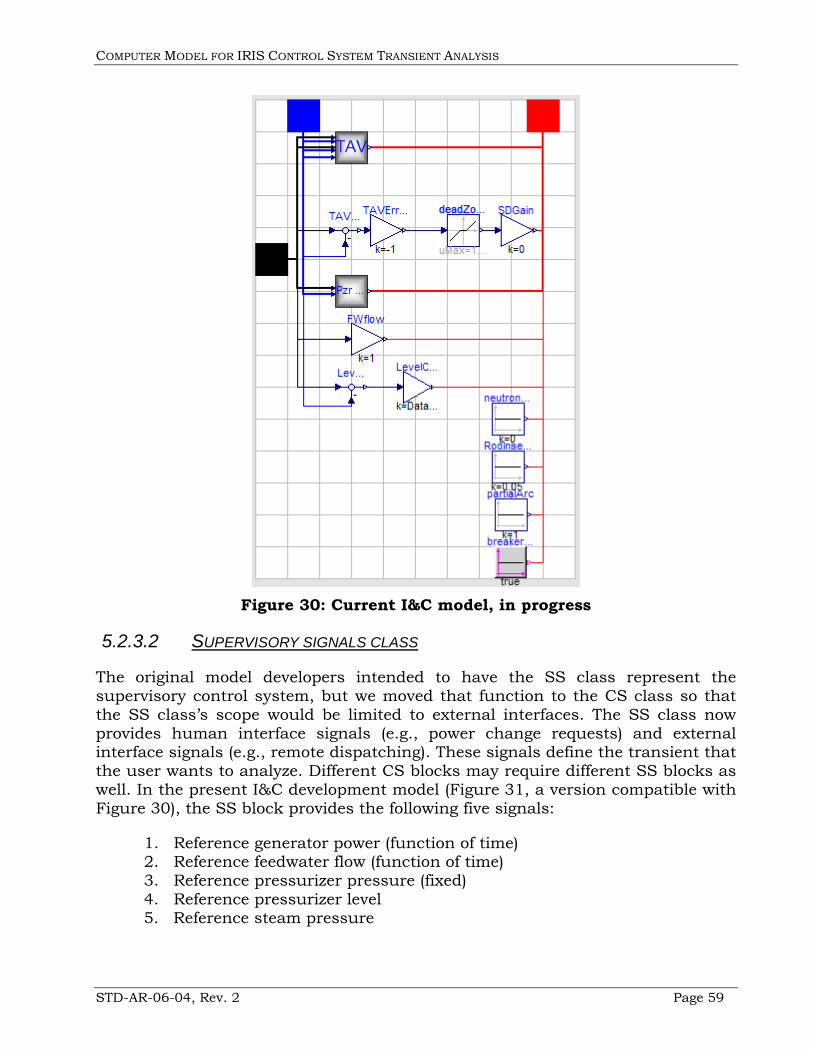
COMPUTER MODEL FOR IRIS CONTROL SYSTEM TRANSIENT ANALYSIS
STD-AR-06-04, Rev. 2 Page 59
Figure 30: Current I&C model, in progress
5.2.3.2 SUPERVISORY SIGNALS CLASS
The original model developers intended to have the SS class represent the supervisory control system, but we moved that function to the CS class so that the SS class’s scope would be limited to external interfaces. The SS class now provides human interface signals (e.g., power change requests) and external interface signals (e.g., remote dispatching). These signals define the transient that the user wants to analyze. Different CS blocks may require different SS blocks as well. In the present I&C development model (Figure 31, a version compatible with Figure 30), the SS block provides the following five signals:
1. Reference generator power (function of time) 2. Reference feedwater flow (function of time) 3. Reference pressurizer pressure (fixed) 4. Reference pressurizer level 5. Reference steam pressure

COMPUTER MODEL FOR IRIS CONTROL SYSTEM TRANSIENT ANALYSIS
STD-AR-06-04, Rev. 2 Page 60
As the control and protection system model advances, so will the SS block model. For example, we plan to eliminate the reference pressurizer level block and replace it with a temperature-dependent level signal calculated in a pressurizer level control block within the CS class. As another example, we will replace the constant reference steam pressure in Figure 31 with a power-dependent calculation.
Figure 31: Supervisory signals
5.2.3.3 SENSORS
Section 5.2.1.1 explained the convention that the NSSS and TGFWS would place pure signals on the sensor bus; i.e., these signals would represent the actual process variable without distortion, noise, or delay. For many studies, these signals are adequate, but eventually analysts will need to account for sensor dynamics. The Sensors_partial_model class accommodates this need by processing signals on the sensor bus and placing them on the measurement bus. Figure 32 shows that the Sensors_partial_model class has a simple structure. One adds additional sensors in the obvious manner. As a partial model, one must provide additional information before use; specifically, one should replace each non-functional GenericSensor with a functional sensor model. Figure 33 shows two such models. The left-hand model is for a trivial sensor, while the right-hand model includes sensor dynamics and limits. The user may construct additional sensor types as needed and may mix sensor types as desired.
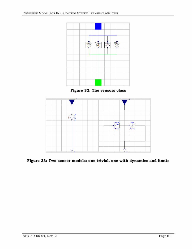
COMPUTER MODEL FOR IRIS CONTROL SYSTEM TRANSIENT ANALYSIS
STD-AR-06-04, Rev. 2 Page 61
Figure 32: The sensors class
Figure 33: Two sensor models: one trivial, one with dynamics and limits

COMPUTER MODEL FOR IRIS CONTROL SYSTEM TRANSIENT ANALYSIS
STD-AR-06-04, Rev. 2 Page 62
6. THE ACSL MODEL
ACSL (pronounced "axle") is the Advanced Continuous Simulation Language. ACSL appeared more than 25 years ago as the first commercially available modeling and simulation language designed for simulating continuous systems. Later versions added discrete-time block capabilities. ACSL follows on the CSSL (Continuous System Simulation Language) standard established by the Technical Committee of the Society for Computer Simulation. Originally, ACSL was solely a text-based programming language, but the latest version, acslXtreme® (Reference 16), includes a graphical programming interface as well.
Westinghouse relied on an earlier version of ACSL during the Temelín I&C development effort. Most of the plant models can be easily adapted to the IRIS, with the notable exception of the steam generator model. Reference 5 describes a moving boundary model for helical coil steam generators that the author implemented in ACSL (this model is the basis for the Matlab/Simulink model described in Section 4.2.2.2.1.2). During the Temelín I&C development effort, Westinghouse took great care to model the I&C Systems in a way that closely followed the actual software coding and execution order. This provided a way to check the final implementation in ways that would not be feasible using Matlab/Simulink or Modelica. On the other hand, developing such an ACSL model is impossible until one selects the final hardware and software platforms and begins detailed implementation; therefore, we leave developing a detailed ACSL model to the future.

COMPUTER MODEL FOR IRIS CONTROL SYSTEM TRANSIENT ANALYSIS
STD-AR-06-04, Rev. 2 Page 63
7. AREAS FOR FURTHER DEVELOPMENT
Identifying areas for further development requires careful appreciation of George P. E. Box’s statement, "All models are wrong-but some models are useful." Answering the question “When will the models be finished?” requires the same appreciation. Experience shows that control system transient analysis models evolve throughout the life of any nuclear I&C project, and that the evolution proceeds as needs evolve. Certainly, the need to develop the control system designs in more detail will dictate model development in the near future. The Matlab/Simulink and Modelica models are already providing useful results. Eventually, we see the Matlab/Simulink model losing importance as the I&C system design stabilizes and the need for detailed analysis increases. Eventually, we hope to construct IRIS plants, and that will require selecting an I&C platform. At that time, we will probably begin using a text-based language in the same way that we used ACSL on the Temelín project. Eventually, the analysis effort will move from design verification to set point selection. Although that involves analyzing the same types of events, the focus and required output format changes. We should be able to say that the models are finished a few months before the final IRIS plant begins its initial power ascension.
COMPUTER MODEL FOR IRIS CONTROL SYSTEM TRANSIENT ANALYSIS
STD-AR-06-04, Rev. 2 Page 64
8. REFERENCES
1. Holcomb, D. E. and A. C. Barroso, “Development of Advanced Instrumentation and Control for an Integrated Primary System Reactor,” Collaborative Proposal for the International Nuclear Energy Research Initiative.
2. Storrick, G. D. and F. Schiavo, STD-ES-04-34, “IRIS Control Systems Conceptual Design,” Sep. 2004.
3. Cammi, A., M. E. Ricotti, F. Cassella, and F. Schiavo, “New modeling strategy for IRIS dynamic response simulation,” 5th International Conference on Nuclear Option in Countries with Small and Medium Electricity Grids, Dubrovnik, Croatia, May 16-20, 2004.
4. Cammi, A., M. E. Ricotti, F. Cassella, F. Schiavo, and G. D. Storrick, “Object-oriented simulation for the control of IRIS nuclear power plant,” IFAC World Congress, Prague, 2005.
5. Information Systems Laboratories, “RELAP5/MOD3.3 Code Manual, Vol 1-8”, NUREG/CR-5535, Rockville, Maryland, USA, 2001.
6. Oriani, L., L.E. Conway, D. Grgic, “Small Break Loss of Coolant Accident Analysis for the International Reactor Innovative and Secure (IRIS),” 5th International Conference on Nuclear Option in Countries with Small and Medium Electricity Grids, May 16-20, 2004, Dubrovnik, Croatia.
7. Grgic, D., L. Oriani, L.E. Conway, “Development Status and Preliminary Validation of a Coupled RELAP/GOTHIC Code for IRIS Small Break LOCA Analysis,” 5th International Conference on Nuclear Option in Countries with Small and Medium Electricity Grids, May 16-20, 2004, Dubrovnik, Croatia.
8. Oriani, L., L.E. Conway, Grgić, D., N. Cavlina, F. Berra, M. Ricotti, G. Ambrogi, F. Oriolo, “IRIS Safety Features and Analysis of Non-Loca Transients and Accidents,”, Global 2003, November 16-20, New Orleans, Louisiana, U.S.
9. T.L. Gorge, et al. “Gothic Containment Analysis Package User Manual”, Version 7.2, NAI-8907-02 Rev 16, Numerical Application Inc., Spring 2004.
10. Maioli, A., D. J. Finnicum, L. Oriani, C. Leva, D. Lamperti, M. Ricotti, “Risk-Informed design process of the IRIS reactor,” International Topical Meeting on Probabilistic Safety Analysis, PSA’05, 11-15 September 2005, San Francisco, California, USA
11. Abdalla, M. A., ORNL/TM-12391, "A nonlinear dynamic model of a once-through helical-coil steam generator," July 1973.

COMPUTER MODEL FOR IRIS CONTROL SYSTEM TRANSIENT ANALYSIS
STD-AR-06-04, Rev. 2 Page 65
12. IEEE Committee Report, 1973, “Dynamic models for steam and hydro turbines in power system studies,” IEEE Transactions on Power Apparatus and Systems, 92, 1905-15.
13. Dynasim AB, “Dymola for Your Complex Simulations,” http://www.dynasim.se/, retrieved September 21, 2006.
14. Cassella, F., “The ThermoPower library Home Page,” http://www.elet.polimi.it/upload/casella/thermopower/, retrieved September 21, 2006.
15. Otter, M. “Modelica,” http://www.modelica.org/library/Modelica/, retrieved September 21, 2006.
16. The AEgis Technologies Group, Inc., “acslXtreme®”, http://www.aegistg.com/AEgisTechnologiesProductsacslXtreme2.html, retrieved September 21, 2006.


![Investigation of Transient Models and Performances for a ... · and transient performances analysis of WTGS[3,4]. Doubly fed induction generators ... doubly fed wind turbines [5]-](https://img.pdfslide.us/doc/110x75/5abf959b7f8b9aa15e8e2fb3/investigation-of-transient-models-and-performances-for-a-transient-performances.jpg)