D352406X012 - Pipeline Thermal Models Remote Automation... · coupled transient ﬂ uid and ground thermal models are compared for pipelines gas and liquid ... Pipeline thermal models

White PaperApril 2016

D352406X012

AbstractHeat fl ow and frictional heating often have a major impact on the hydraulics of a pipeline. An accurate pipeline simulation frequently needs some form of thermal model. Many different approaches are in common use for these models, ranging from a simple assumption of isothermality to detailed transient models of heat fl ow in the fl uid, pipe wall, and surrounding material. Elaborate thermal models can be diffi cult to create and time-consuming to execute, so it is important to understand the level of detail needed for a given application.

This paper investigates the impact of the thermal model on the overall pipeline model accuracy, especially on the linepack (for gas pipelines) and throughput. The isothermal assumption, various types of transient and steady-state fl uid thermal models, and coupled transient fl uid and ground thermal models are compared for pipelines gas and liquid pipelines.

IntroductionEvery pipeline simulation must include some sort of thermal model. This can be as simple as an assumption that the fl uid in the pipe is always at a fi xed temperature, or as complex as a fullblown transient model that calculates heating and energy fl ow in both the fl uid and the ground. For some applications, the results of a pipeline model depend heavily on the accuracy of the associated thermal model; in other cases, an “isothermal” (constant temperature) model is perfectly suffi cient.

This article evaluates several techniques for fl uid and ground thermal modeling with an eye to applicability to common calculations on gas and liquid pipelines. The goal is to determine the level of error that can be expected with different thermal modeling approaches for capacity calculations, linepack calculations, survival-time analysis, and leak detection.

Pipeline Thermal ModelsJason Modisette, Ph.D., Emerson (formerly Energy Solutions Int’l.)

Midstream Oil and Gas Solutions

2 www.EmersonProcess.com/Remote

April 2016

First, the physics of thermal behavior of fl uid fl owing (or sitting) in pipes will be briefl y covered. Then, the components of a complete thermal model will be described and compared with common approximations. The equations used for calculating heat fl ow into and inside the ground also are important parts of the thermal model; two ways of modeling the heat fl ow into and within the ground will be discussed.

The accuracies of the different fl uid and ground thermal models will be compared. Next, there will be a discussion of the effects of poor knowledge of diffi cult-to-predict quantities such as ground temperature and ground thermal conductivity on the models’ accuracies. The fanciest thermal model is only as good as the data used to drive it, which often is not very good.

Thermal Behavior of Fluids in PipesThermal models based on different approximations have varying degrees of success at handling different thermal phenomena. Before going into the details of the different types of commonly used thermal models, those effects that will be examined in this article are described.

An important channel of thermal energy loss from the fl uid is conduction into the ground through the pipe wall. This process can be critical to the operation of a pipeline: for example, certain crude pipelines would be essentially destroyed as the crude turned into tar, if this process were allowed to proceed to equilibrium when the fl ow is stopped. To the pipeline modeler, the ground outside the pipe is a mysterious thing: it can have widely varying thermal properties depending on, for example, how long it has been since the last rain. Errors introduced into thermal models by poor knowledge of ground thermal properties will be discussed below; all errors coming from the various approximations should be compared with these inevitable errors caused by such unknown factors when determining the correct thermal model for a given application.

Underwater pipelines (especially uncovered lengths such as the vertical spans leading from a drilling rig down to the sea fl oor) must consider not only conduction but convection as well, which is the primary method of heat transfer from a hot object submerged in water.

As gas or oil fl ows down a pipe, it loses momentum to friction with the wall. This results in a corresponding loss of kinetic energy, which (according to the conservation of energy) must go somewhere: either into the fl uid as heat, or into the wall as heat. Convection by the fl uid is a much more effi cient method of transporting the heat away than conduction into the wall, with the result that essentially all of the frictional heat goes into the fl uid.

Different thermal processes occur on different timescales. Several assumptions are made in pipe thermal models based on this fact. Conduction is usually much slower than convection, for example, which means that simpler numerical methods can be used to model how heat fl ows within the ground than the methods needed for accurate modeling of all the processes in the fl uid itself. However, one must be careful: the ground takes much longer to come to steady-state than the fl uid would by itself, which means that the succession-of-steady-states approximation is even less appropriate to ground thermodynamics than it is when applied to the fl uid.

The Energy EquationPipeline thermal models are usually based on the law of conservation of energy. This law states that the total energy in the pipeline is neither created nor destroyed - it can be added (usually by compressors or pumps) or removed (heat fl ow to the ground) or can change form (for instance, during expansion of a non-ideal gas, work done against the attractive forces between molecules can result in cooling) but it never vanishes or appears from nowhere.

This law can be applied to a small volume of length dx and the pipe’s cross-sectional area A. Just as the energy does not appear or disappear in the pipeline as a whole, it also does not do so in each such chunk of fl uid. Therefore, the rate of change of energy each volume of fl uid must equal the rate energy is fl owing into/out of that volume.

www.EmersonProcess.com/Remote 3

Midstream Oil and Gas SolutionsApril 2016

The law of conservation of energy can be written as a partial differential equation that applies to each element of fl uid in the pipeline. The temperature is a measure of one part of the internal energy of a fl uid. For an ideal gas, the temperature represents all of the internal energy, but in real gases and liquids some of it is tied up in intermolecular forces. The mathematical statement of conservation of energy, called the “energy equation”, can thus be solved for the temperatures in the pipeline.

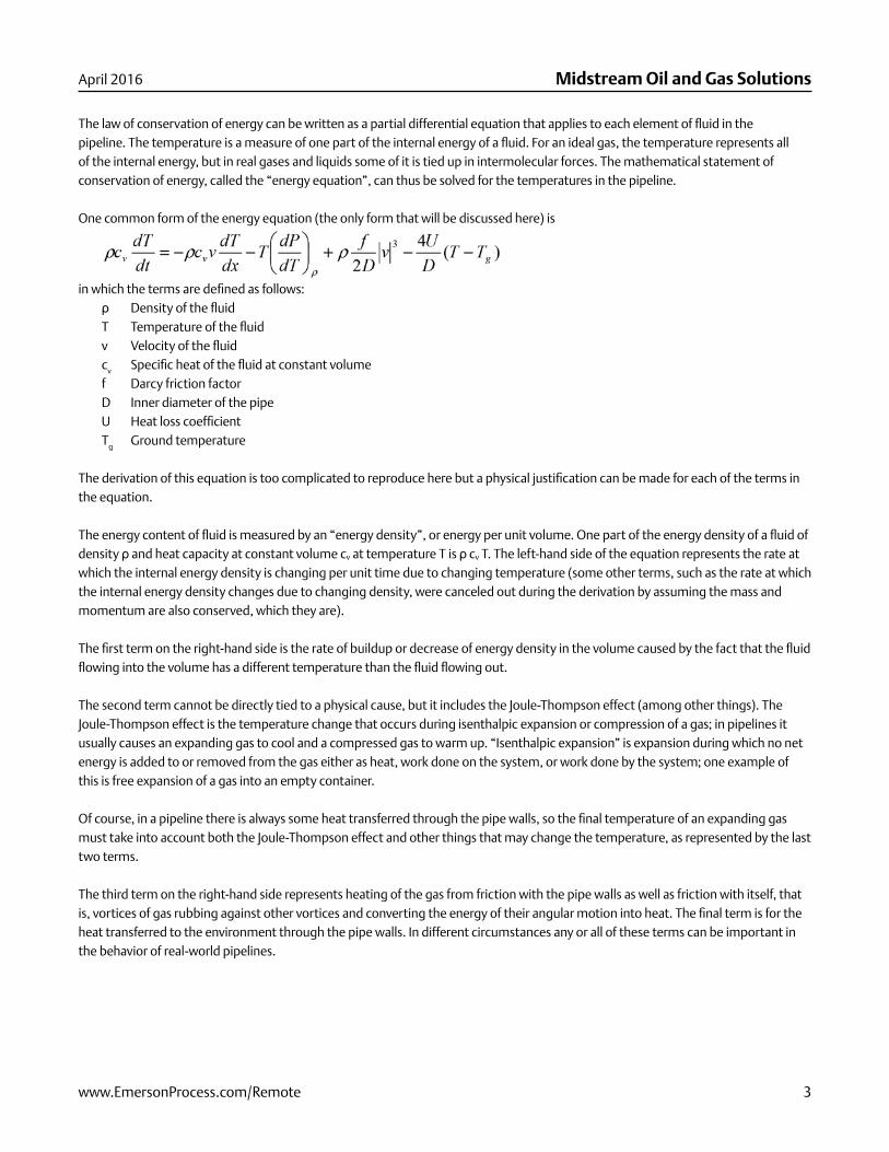
One common form of the energy equation (the only form that will be discussed here) is

in which the terms are defi ned as follows:ρ Density of the fl uidT Temperature of the fl uidv Velocity of the fl uidcv Specifi c heat of the fl uid at constant volumef Darcy friction factor D Inner diameter of the pipeU Heat loss coeffi cientTg Ground temperature

The derivation of this equation is too complicated to reproduce here but a physical justifi cation can be made for each of the terms in the equation.

The energy content of fl uid is measured by an “energy density”, or energy per unit volume. One part of the energy density of a fl uid of density ρ and heat capacity at constant volume cv at temperature T is ρ cv T. The left-hand side of the equation represents the rate at which the internal energy density is changing per unit time due to changing temperature (some other terms, such as the rate at which the internal energy density changes due to changing density, were canceled out during the derivation by assuming the mass and momentum are also conserved, which they are).

The fi rst term on the right-hand side is the rate of buildup or decrease of energy density in the volume caused by the fact that the fl uid fl owing into the volume has a different temperature than the fl uid fl owing out.

The second term cannot be directly tied to a physical cause, but it includes the Joule-Thompson effect (among other things). The Joule-Thompson effect is the temperature change that occurs during isenthalpic expansion or compression of a gas; in pipelines it usually causes an expanding gas to cool and a compressed gas to warm up. “Isenthalpic expansion” is expansion during which no net energy is added to or removed from the gas either as heat, work done on the system, or work done by the system; one example of this is free expansion of a gas into an empty container.

Of course, in a pipeline there is always some heat transferred through the pipe walls, so the fi nal temperature of an expanding gas must take into account both the Joule-Thompson effect and other things that may change the temperature, as represented by the last two terms.

The third term on the right-hand side represents heating of the gas from friction with the pipe walls as well as friction with itself, that is, vortices of gas rubbing against other vortices and converting the energy of their angular motion into heat. The fi nal term is for the heat transferred to the environment through the pipe walls. In different circumstances any or all of these terms can be important in the behavior of real-world pipelines.



April 2016

Heat Flow in the GroundHeat conduction in any material is described by Fourier’s Law of Heat Conduction,

in which the variables are defi nedq Heat fl ux (heat fl ow per unit area)k Thermal conductivity of the materialT Temperature

This equation can be used to determine the heat fl ow around pipelines. In most circumstances conduction is the only important mechanism by which heat leaves the pipeline through the pipe walls. In the case of a pipeline that’s either directly in contact with water, or has a small amount of insulating material between itself and water, other effects such as free convection (convection driven by the buoyancy of hotter fl uid, which also causes updrafts in the air over exposed rock and the fl ow patterns in a hot cup of coffee) can become important. Convection can be modeled accurately with a “fi lm heat transfer coeffi cient” C that relates the rate of heat loss to the temperature difference between the water and the pipe, as follows:

Q Heat fl ow from pipe to waterC Film heat transfer coeffi cientTpipe Temperature of the pipeT water Temperature of the water

where C is a function of the details of the problem. This article will not address free convection any further: it will be assumed that conduction is the only important mechanism for heat to escape from the pipeline along its length.

Steel pipe has a high thermal conductivity (50 to 500 times higher than soil) and during turbulent pipe fl ow is in good thermal contact with the fl uid, so to a very good approximation both the pipe and the fl uid are at a uniform temperature. This will be assumed for the rest of this article (this assumption may not hold when fl ow is stopped; then the fl uid may not be at a constant temperature and will generally have a lower rate of heat loss than when fl owing). It is important to include the heat capacity of the pipe along with the heat capacity of the fl uid in the fl uid thermal model when making this assumption.

Numerical Approaches: Fluid Thermal ModelsOver the last thirty years a wide variety of different models have been used to enforce the energy equation. First, a full thermal model will also be considered, in which the coupled energy, mass, and momentum equations are all solved at the same time along with the transient ground heat fl ow equations. This model is the most complete of those examined here and will therefore be referred to as the “correct” model, but it is still subject to bad data and to those approximations mentioned in earlier sections. Next, four of the most common approximations to this model will be described: the isothermal approximation, a succession-of-steady-states approach, a “leapfrog” transient thermal model with fi xed knots which alternates solution of the hydraulic model and solution of the thermal model, and an analytical solution of the thermal equations with moving knots (“knots” are the points at which the temperature is calculated).

Full Model (Coupled Transient Thermal and Hydraulic Models)A complete pipeline model is governed by three differential equations, which come from conservation of mass, conservation of momentum, and conservation of energy. The simultaneous solution of these three equations is the state of the fl uid in the pipeline, which consists of values everywhere for the fl ow rate, pressure, and temperature. These equations can be solved numerically, but for a numerical solution to be strictly correct it must solve all three equations simultaneously. This is commonly not done in the pipeline



industry: the mass and momentum equations are solved in one pass, and then some other approach is used for the thermal model. The errors introduced by this separation will be described below.

There are various numerical approaches that can be used to solve the coupled partial differential equations. In this article a fully implicit approach will be used with a small amount of artifi cial viscosity to improve the models stability in the face of sudden changes in boundary conditions. Explicit and semi-implicit (box method or Crank-Nicholson) numerical solutions have also been applied successfully to these equations. The reader who is unfamiliar with these different numerical methods should be assured that no understanding of them is needed in order to follow the remainder of this article.

Even though this model is referred to here and below as the “correct” model, it is still subject to inaccuracies in both the data (ground temperatures and especially ground thermal conductivities) and the numerical limits of the ground thermal model. In addition, all of the possibilities for numerical solution of the energy equation introduce some amount of “numerical dispersion”; this means that a sharp temperature front caused, for example, by turning on an injection of a hot stream into an existing cold stream, will tend to be “washed out” over distance. This defect is addressed by one of the approximations listed below, the moving-knots pseudosteady model. In many cases, the coupling between the fl uid temperature and the ground produces similar “washing-out” effects, which are physically real.

The Isothermal ApproximationThe isothermal approximation is made when a pipeline simulation has no formal thermal model, but simply assumes that the temperature is known. This approach usually assumes a constant temperature everywhere in the pipe. There are also pipeline models in use that assume a temperature profi le that is unchanging with time but that does vary over space; however, for brevity only the former type of model will be considered here. In tests done below, a “reasonable” but constant temperature is assumed for the isothermal approximation.

The source of errors in the isothermal approximation is obvious: it does not make any attempt to solve for the temperatures in the pipeline, but simply uses an educated guess. To the extent that this guess is incorrect, it produces errors in the model.

Succession of Steady-StatesIn many pipeline networks (especially liquid pipelines) it is numerically effi cient to solve the model equations by integrating them from one boundary to the other, rather than by one of the standard matrix techniques. This approach has the advantages of being comparatively easy to code and fast to solve. The technique lends itself better to steady-state solutions than to transient solutions (although it can be implemented for transient models as well).

This has led to a number of pipeline models that solve the steady-state energy equation at each timestep. The steady-state energy equation is just Equation 1 with the left-hand side set equal to zero. Since this removes the time-dependence from the equation, it can now be integrated over x.

There are two drawbacks to this approximation: the fi rst, which is shared by all four of the approximate models described here, is that the energy equation is no longer correctly coupled to the other model equations (this defi ciency goes away when this thermal model is used with a succession-of-steady-states hydraulic model, but that brings a host of other problems). The second is that much of the time, the dominant thermal effects in pipelines occur as fl uid of a different temperature (or, in liquid pipelines, of different physical properties) is carried down the pipe. Since this approximation treats the pipeline as if it reaches steady-state after each model time-step, it does not correctly catch the effects of thermal “fronts”, bodies of fl uid of different temperature, moving through the system. This can result in signifi cant temperature errors that persist for many hours.



April 2016

Leapfrog Transient ModelThe energy equation can be solved exactly, but independently of the mass and momentum equations instead of simultaneously with them. This type of model will be referred to as a “leapfrog” thermal model, since it alternates solving hydraulic and thermal equations as time advances. Each solution of the energy equations computes temperatures from the previous values of pressure and fl ow, and each hydraulic model solution computes pressures and fl ow rates from the previous values of temperature.

The advantage of this model over the correct combined transient hydraulic and thermal model is one of speed: it’s faster to invert two small matrices than one big matrix. Because of the structure of the matrices in this case, this holds even when using a sparse matrix solver. Speed is less of an issue with modern computers, but for offl ine models it is still desirable to run at as high a multiple of real time as possible.

The only drawback to this model is that some approximation must be made for the next-step temperatures that appear in the hydraulic model (these temperatures appear implicitly in the mass and momentum conservation equations, because the density and viscosity of the fl uid are used in these equations and those are both functions of temperature). The most straightforward approximation is to use the same temperature for computing the next-step and previous-step properties, but the author has found this to introduce major errors in the results of the hydraulic model. The results given below, which agree quite well with the “correct” model, use a linear extrapolation of the next-step temperature from the previous two steps.

Pseudo-Steady Model with Moving KnotsThere is a middle ground between a fully transient solution and a purely steady-state solution: the temperature of each element of fl uid can be evolved each model step as if it had moved through hydraulic steady-state conditions of whatever the transient hydraulic model is currently showing for its vicinity. This keeps the transient behavior of the fi rst term on the right hand side of the energy equation, but loses the transient behavior associated with the remaining terms.

Since timesteps in a transient pipeline model are usually of such a length that an element of fl uid does not move all the way from one knot to the next over a timestep, it’s necessary to track the thermal knots separately for this type of approach. The easiest way to implement this is to let the knots move along the pipe at each step. This allows analytical solution of Equation 1 with the assumption that the various terms on the right-hand side (other than the temperature itself) are temperature-independent. That is, they are steady at whatever the hydraulic model said they were, rather than changing with time - thus, this is a kind of steady-state assumption. The two terms in the energy equation for which this is a suspicious assumption are velocity and the dP/dT term. As long as the fl uid is moving, this model turns out to be fairly safe for liquids (at least in the test cases run by the author), but in general a correct model is preferable.

For an ideal gas, T (dP/dT)ρ is independent of temperature (it turns out to be a constant multiplied by the pressure). This means that the temperature dependence of that term for real gases will generally be small, and proportional to how rapidly the z factor varies with temperature. However, the velocity change with temperature goes approximately as the inverse of the density change, which is linear in temperature. That means that the velocity change is proportional to the fractional temperature change. A temperature variation over one model step of 1°F for a room-temperature gas that translates to about a 0.2% velocity error.

This type of model has the advantage, just like the succession of steady-states model, of not requiring any matrix inversions - it can be implemented using analytical solutions only. This makes it faster and easier to implement than the “correct” model. Its main disadvantage is that it does not provide an accurate representation of the dP/dT term in the energy equation in changing conditions, and can therefore miss certain transient effects. For example, in a gas pipeline a compressor startup can result in a short slug of heated fl uid caused by the compression of the initially low-pressure gas immediately downstream of the compressor. This type of model will not reproduce that effect.



Numerical Approaches: Ground Thermal ModelsThe ground thermal model can be viewed as completely independent of the fl uid thermal model except for the values of Tg and U in Equation 1. This is possible because the temperature in the ground changes slowly compared to the temperature in the fl uid. The fl uid temperature is dominated by the convection of the fl uid down the pipeline, while the ground temperature is governed entirely by conduction.

The exception to this occurs for underwater pipes. Then, signifi cant convection can occur in the water heated by the pipe, or a current fl owing across the pipe can carry heat away.

As long as only conduction is important, the ground heat fl ow follows a diffusion equation. Diffusion equations are relatively easy to solve numerically either in steady-state or transient modes. All that is needed is a description of the geometry of the region of interest (the ground near the pipeline) and a choice of boundary conditions.

Geometry and Boundary ConditionsMost ground thermal models treat the ground as a set of concentric cylindrical shells. Since the pipe is also a cylinder, this reduces the ground heat fl ow problem to a one-dimensional equation at each model knot along the pipe. The effects of conduction of heat in the ground along the pipe are generally ignored, as they should be: the fl uid fl ow in the pipe is so much more effi cient at carrying heat along the pipe than conduction through the ground that such conduction is completely negligible. This means that the ground thermal model at each point along the pipe is independent of the ground thermal models at the other points.

In any ground thermal model some assumption must be made about outer boundary conditions. The usual assumption is that there is a constant temperature on the outside of the outermost shell, which is fi xed at some typical ambient temperature. This approximation is fairly safe as long as the size of the shells is less than one or two pipe diameters, but is increasingly suspicious for larger volumes. There is a competing effect, however, which is that close to the pipe the temperature may be constant around the circumference of the shell but it’s no longer constant over time. Nonetheless, this is an almost ubiquitous approximation since the alternative is to lose cylindrical symmetry and that necessitates a much more diffi cult numerical solution.

The author has found that the details of the outer boundary of the ground thermal model, its temperature and location, are relatively unimportant compared to the sizes and thermal conductivities of the inner shells. In steady-state, the rate of heat loss from the pipe is proportional to the difference between the fl uid temperature and the outer ground temperature divided by the log of the ratio of the outer ground thermal boundary to the radius of the pipe. This means that the rate of heat loss changes very slowly as the outer boundary‘s distance is increased.

Steady-StateThe ground reaches thermal equilibrium much more slowly than the pipe does, so a steady-state approximation is that much worse than a steady-state approximation for the fl uid. However, as is the case with the fl uid steady-state thermal model, this is the easiest solution to derive and program, and therefore is common.

A steady-state ground thermal model essentially just amounts to a thermal resistance linking the fl uid to a fi xed ground temperature; Fourier’s law (Equation 2) can be used to calculate the heat fl ow rate. Any conceivable geometry will still result in this same equation, with only the value of the constant k changing. This can then be directly applied to Equation 1 or its steady-state counterpart, where the inverse of that resistance appears as U.

Analytical steady-state solutions for U are known for sets of concentric cylinders and also for a cylinder near a half-plane; this latter case is a good description of the geometry of a buried pipe. As stated above, the exact details of the outer boundary do not have a



April 2016

strong effect on the heat loss from the pipe. It is common to use the burial depth of the pipe as an outer boundary distance, since clearly any more distant boundary would be non-physical.

TransientRather than assuming a constant ground temperature, the heat content in the ground can be tracked over time. Ground thermal models that use this approach are called transient ground thermal models (analogously to pipeline models that include the correct physics of rates of change of pressure, temperature, and fl ow rate). Because the timescale of ground thermal diffusion is very slow compared to the typical maximum timestep used in pipeline models, if the ground thermal model is run every model step, or even every few model steps, then most numerical solution techniques will be stable.

Note that if the pipe temperature is tracked as part of the transient ground thermal model, it may not be accurate. This is because the pipe generally reaches the fl uid temperature orders of magnitude faster than the ground does.

Choosing the spacing of ground thermal shells is a function of experiment more than abstract principles. It’s generally a good idea to have thin shells (one inch or so) close to the pipe and thicker shells farther away. The details of the outer shells are usually relatively unimportant. For tests done below, three one-inch-thick shells surround the 30-inch-diameter pipe, followed by a four-inch shell and a 35-inch thick shell, all made of the same material. This set was the result of some trial and error; the other extreme of a single 43-inch thick shell resulted in differences of up to 3°F over about ten miles from the chosen set of shells. For accuracy it was important to have at least one fairly thin shell close to the pipe.

Accuracy ComparisonsThe important thermal effects are quite different for gas and liquid pipelines. With heavy crudes, the viscosity can change rapidly with changing temperature, which causes relatively small temperature errors to balloon into large pressure drop errors. Thermal viscosity effects in products are smaller and can be relatively unimportant. In gases, the thermal effects on viscosity are quite small, but the density scales linearly with the temperature. This affects both the linepack and the frictional pressure loss.

In circumstances such as line ruptures where gas pipelines undergo rapid depressurization, Joule-Thomson cooling becomes the dominant thermal phenomenon. Accurate thermal modeling is extremely important for studies of rapid pressure loss because the temperature determines whether hydrates form and whether the steel of the pipe becomes brittle. Unfortunately there are many complicating factors in studies of ruptures, so for this article a simpler system is being studied: the survival time of a gas pipeline under an increase in demand with no accompanying increase in supply. This allows similar thermal effects to be modeled while avoiding problems of multi-phase or supersonic fl ow.

ResultsThe various thermal models have been used to simulate several steady and transient scenarios for both gas and liquid pipelines. For steady operation of a gas pipeline, the throughput and linepack have been computed. They have also been computed for a transient scenario in which a compressor starts up at the head of the line. Finally, a gas scenario in which a delivery suddenly increases its demand has been modeled to compute survival time until the delivery drops below minimum pressure.

For a liquid pipeline, the different thermal models are used to calculate the steady-state throughput fl ow rate, as well as the packing rate under transient conditions of pump startup (a quantity of interest to leak-detection applications).

Simulation DetailsAll tests were performed on single 30-mile long pipes with 30” inner diameter. Gas tests used pressure-pressure boundaries except where otherwise specifi ed. The gas model used a 30-second timestep and 1-mile knot spacing. Gas entered the system at 90 F, and the ground temperature was 50 F. The NX-19 equation of state was used, with a gas with an average molecular weight of 18.9.



In gas simulations with a “compressor start”, the compressor was not modeled exactly but instead the startup was simulated with a 100-psi pressure increase and a 10°F temperature increase at the supply over a period of 2 minutes. Liquid simulations used a high-viscosity crude oil, using API correlations for the equation of state. Since transient effects occur more rapidly in liquids than in gases, a 5 second model timestep was used. The same 1-mile knot spacing was used.

All tests used a hydraulic model that performs an implicit solution of the mass and momentum equations, either coupled with the thermal equations or alternating with the thermal equations as required by the particular thermal model. Steady-state simulations with uncoupled thermal models iterated the hydraulic and thermal model three times, which was always enough to converge the results to more than the number of fi gures reported here. It is not recommended that an uncoupled thermal model be used for steady-state results without at least one additional iteration, as the thermal results from the fi rst pass of the uncoupled thermal model in steady-state contain major deviations from the correct results.

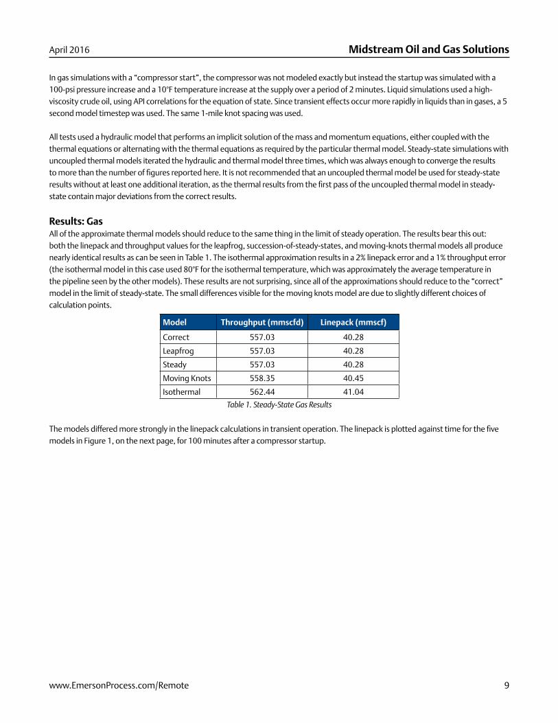
Results: GasAll of the approximate thermal models should reduce to the same thing in the limit of steady operation. The results bear this out: both the linepack and throughput values for the leapfrog, succession-of-steady-states, and moving-knots thermal models all produce nearly identical results as can be seen in Table 1. The isothermal approximation results in a 2% linepack error and a 1% throughput error (the isothermal model in this case used 80°F for the isothermal temperature, which was approximately the average temperature in the pipeline seen by the other models). These results are not surprising, since all of the approximations should reduce to the “correct” model in the limit of steady-state. The small differences visible for the moving knots model are due to slightly different choices of calculation points.

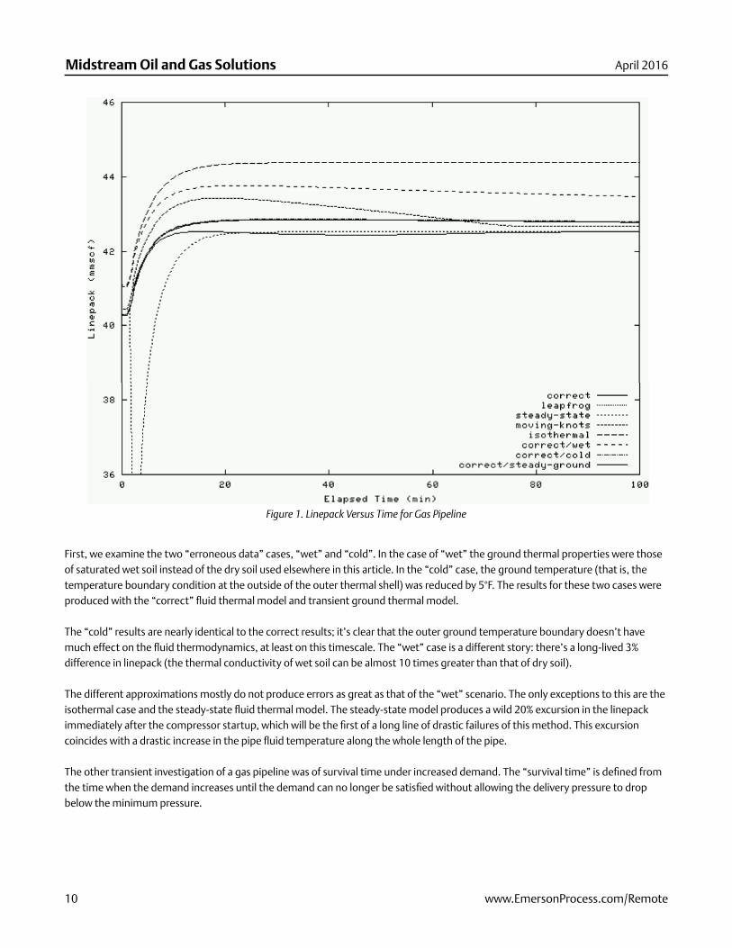
The models differed more strongly in the linepack calculations in transient operation. The linepack is plotted against time for the fi ve models in Figure 1, on the next page, for 100 minutes after a compressor startup.

Model Throughput (mmscfd) Linepack (mmscf)

Correct 557.03 40.28

Leapfrog 557.03 40.28

Steady 557.03 40.28

Moving Knots 558.35 40.45

Isothermal 562.44 41.04

Table 1. Steady-State Gas Results



April 2016

First, we examine the two “erroneous data” cases, “wet” and “cold”. In the case of “wet” the ground thermal properties were those of saturated wet soil instead of the dry soil used elsewhere in this article. In the “cold” case, the ground temperature (that is, the temperature boundary condition at the outside of the outer thermal shell) was reduced by 5°F. The results for these two cases were produced with the “correct” fl uid thermal model and transient ground thermal model.

The “cold” results are nearly identical to the correct results; it’s clear that the outer ground temperature boundary doesn’t have much effect on the fl uid thermodynamics, at least on this timescale. The “wet” case is a different story: there’s a long-lived 3% difference in linepack (the thermal conductivity of wet soil can be almost 10 times greater than that of dry soil).

The different approximations mostly do not produce errors as great as that of the “wet” scenario. The only exceptions to this are the isothermal case and the steady-state fl uid thermal model. The steady-state model produces a wild 20% excursion in the linepack immediately after the compressor startup, which will be the fi rst of a long line of drastic failures of this method. This excursion coincides with a drastic increase in the pipe fl uid temperature along the whole length of the pipe.

The other transient investigation of a gas pipeline was of survival time under increased demand. The “survival time” is defi ned from the time when the demand increases until the demand can no longer be satisfi ed without allowing the delivery pressure to drop below the minimum pressure.

Figure 1. Linepack Versus Time for Gas Pipeline



Survival times were investigated for the same pipeline as used above.

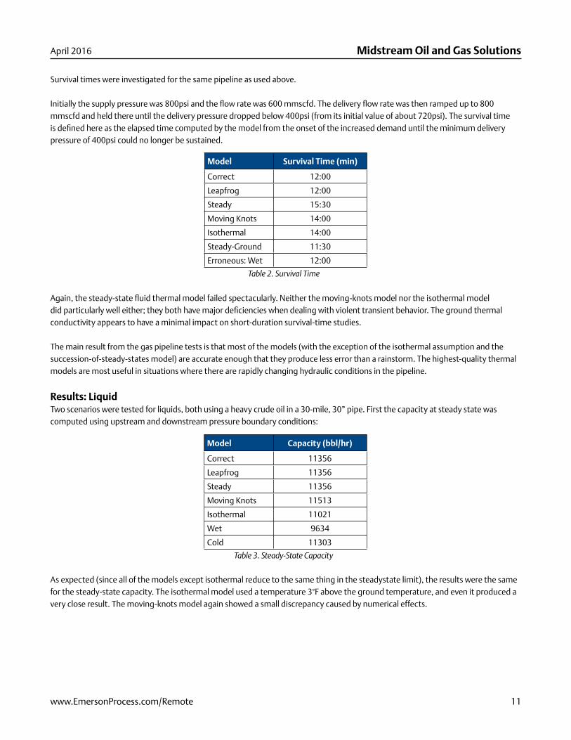
Initially the supply pressure was 800psi and the fl ow rate was 600 mmscfd. The delivery fl ow rate was then ramped up to 800 mmscfd and held there until the delivery pressure dropped below 400psi (from its initial value of about 720psi). The survival time is defi ned here as the elapsed time computed by the model from the onset of the increased demand until the minimum delivery pressure of 400psi could no longer be sustained.

Again, the steady-state fl uid thermal model failed spectacularly. Neither the moving-knots model nor the isothermal model did particularly well either; they both have major defi ciencies when dealing with violent transient behavior. The ground thermal conductivity appears to have a minimal impact on short-duration survival-time studies.

The main result from the gas pipeline tests is that most of the models (with the exception of the isothermal assumption and the succession-of-steady-states model) are accurate enough that they produce less error than a rainstorm. The highest-quality thermal models are most useful in situations where there are rapidly changing hydraulic conditions in the pipeline.

Results: LiquidTwo scenarios were tested for liquids, both using a heavy crude oil in a 30-mile, 30” pipe. First the capacity at steady state was computed using upstream and downstream pressure boundary conditions:

As expected (since all of the models except isothermal reduce to the same thing in the steadystate limit), the results were the same for the steady-state capacity. The isothermal model used a temperature 3°F above the ground temperature, and even it produced a very close result. The moving-knots model again showed a small discrepancy caused by numerical effects.

Model Survival Time (min)

Correct 12:00

Leapfrog 12:00

Steady 15:30

Moving Knots 14:00

Isothermal 14:00

Steady-Ground 11:30

Erroneous: Wet 12:00

Table 2. Survival Time

Model Capacity (bbl/hr)

Correct 11356

Leapfrog 11356

Steady 11356

Moving Knots 11513

Isothermal 11021

Wet 9634

Cold 11303

Table 3. Steady-State Capacity



April 2016

The impact of wet ground on the fl ow rate in this system is an immense 14%. This is because in equilibrium the hot crude loses more heat to the wet ground than dry, and therefore is at a lower average temperature. This increases the viscosity and thus the frictional head losses drastically.

Leak detection is one of the applications most demanding of accuracy in pipeline models. Leak detection applications often work by computing a modeled “packing rate”, which is the total fl ow rate into the pipeline minus the total fl ow rate out of the pipeline. In steady operations the packing rate is zero; a leak can be identifi ed as a deviation of the modeled packing rate from the packing rate reported by fl ow meters (this is just one of many ways of detecting leaks, but the packing rate is used by several common methods). Errors in the modeled packing rate are one limiting factor on the sensitivity of leak detection. For example, if there are frequent 1% errors in the modeled packing rate that persist for 30 minutes, then the system won’t be able to detect a 1% leak in less than 30 minutes, because it won’t know if a smaller leak is real or is an artifact of the model.

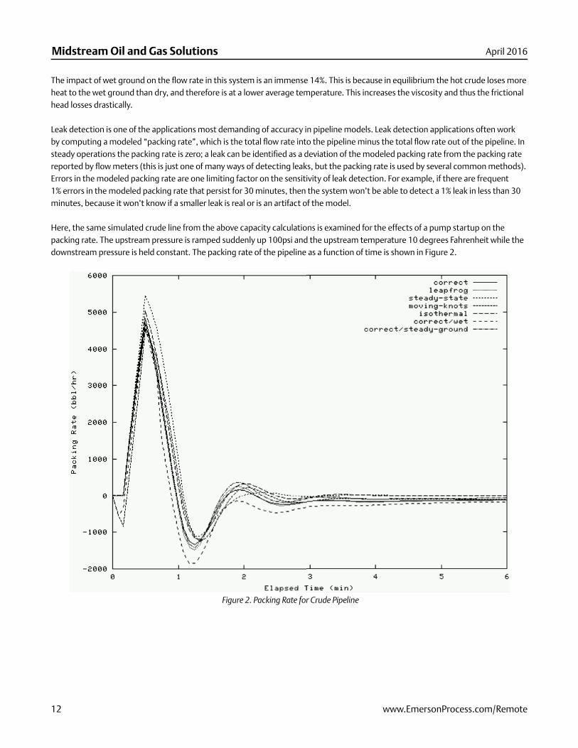
Here, the same simulated crude line from the above capacity calculations is examined for the effects of a pump startup on the packing rate. The upstream pressure is ramped suddenly up 100psi and the upstream temperature 10 degrees Fahrenheit while the downstream pressure is held constant. The packing rate of the pipeline as a function of time is shown in Figure 2.

Figure 2. Packing Rate for Crude Pipeline



This fi gure again shows the importance of having an accurate ground thermal conductivity; the wet-soil scenario produces worse errors than do any of the various physical approximations. Several interesting phenomena are visible here. The isothermal and succession-of-steadystates fl uid thermal model don’t track the large surges well, and then they go quickly to a packing rate of zero. The other models are all coupled with a transient ground thermal model, and therefore experience the correct long-term ground thermal behavior (except for the wet-soil scenario). The packing rate remains above 100 bbl/hr for those models (and presumably for the real pipeline) for another three hours. This refl ects the time it takes the fl uid to heat up the ground and reach its fi nal temperature.

ConclusionOne consistent result for most of the models in both gas and liquid simulations has been that the errors caused by the model were smaller than the error that caused by the difference in ground thermal conductivity between dry and wet soil. The only model for which this isn’t true is the succession-of-steady-states model. It produced signifi cantly worse errors than any of the others, because of its unique ability to instantly (and wrongly) propagate a short-lived temperature increase down the entire line. The author recommends that this sort of thermal model not be used for transient studies, even coupled to a fully transient hydraulic model. The modeler would probably be better off with an isothermal approximation.

The moving-knots thermal model, while it didn’t produce huge errors, wasn’t particularly accurate and missed some signifi cant transient effects in gases. This method is also not recommended, because it doesn’t provide any meaningful benefi t over the more accurate fi xed knot models. The diffusion of thermal fronts that it avoids tends to happen to some extent in reality due to coupling between the fl uid temperature and the ground temperature immediately around the pipe.

It appeared to make little difference whether the energy equation was solved at the same time as the mass and momentum equations, or in alternating steps. In order to get this agreement, it is necessary to include in the hydraulic model terms accounting for the rate of change of temperature with time; computing these terms by linear extrapolation of past temperatures (the method used above) was found to produce accurate results even in rapidly changing conditions.

The soil thermal conductivity turned out to have a great infl uence on the model results. In offl ine engineering studies it is best to use several different possible soil types (wet, dry, etc.) to explore the different operating conditions of the pipeline; the differences can be signifi cant. In online applications, especially those like leak detection that require a highly accurate model, the ground thermal conductivity should be tuned automatically to correct for the effect of weather on soil moisture content.

In conclusion, the author recommends that applications requiring model accuracy better than that that can be obtained with an isothermal approximation should use a fully transient solution of the energy equation and especially a fully transient ground thermal model.

About the AuthorJason Modisette earned his B.S. in Physics from the California Institute of Technology and his Ph.D. in Physics from Rice University, where he wrote numerical models for quantum chemistry problems. He has worked at Emerson, where he currently holds the post of Technical Director, since 1997. At Emerson, he has developed an offl ine batched liquid pipeline scheduling and optimization program and a real-time gas model. He is currently working on the next release of TGNET, an offl ine gas model.

RemoteAutomationSolutions

Remote Automation Solutions Community

Global HeadquartersNorth America and Latin AmericaEmerson Process ManagementRemote Automation Solutions6005 Rogerdale RoadHouston, TX, USA 77072T +1 281 879 2699 F +1 281 988 4445

www.EmersonProcess.com/Remote

EuropeEmerson Process ManagementRemote Automation SolutionsUnit 8, Waterfront Business ParkDudley Road, Brierley HillDudley, UK DY5 1LXT +44 1384 487200 F +44 1384 487258

Middle East and AfricaEmerson Process ManagementRemote Automation SolutionsEmerson FZEPO Box 17033Jebel Ali Free Zone - South 2Dubai, UAET +971 4 8118100 F +1 281 988 4445

Asia PacificEmerson Process ManagementAsia Pacific Private LimitedRemote Automation Solutions1 Pandan CrescentSingapore 128461T +65 6777 8211F +65 6777 0947

D352406X012 / Printed in USA / 04-16

Find us around the corner or around the worldFor a complete list of locations please visit us at www.EmersonProcess.com/Remote

© 2016 Remote Automation Solutions, a business unit of Emerson Process Management. All rights reserved.

Emerson Process Management Ltd, Remote Automation Solutions (UK), is a wholly owned subsidiary of Emerson Electric Co. doing business as Remote Automation Solutions, a business unit of Emerson Process Management. FloBoss, ROCLINK, ControlWave, Helicoid, and OpenEnterprise are trademarks of Remote Automation Solutions. AMS, PlantWeb, and the PlantWeb logo are marks owned by one of the companies in the Emerson Process Management business unit of Emerson Electric Co. Emerson Process Managment, Emerson and the Emerson logo are trademarks and service marks of the Emerson Electric Co. All other marks are property of their respective owners.

The contents of this publication are presented for informational purposes only. While every effort has been made to ensure informational accuracy, they are not to be construed as warranties or guarantees, express or implied, regarding the products or services described herein or their use or applicability. Remote Automation Solutions reserves the right to modify or improve the designs or specifications of such products at any time without notice. All sales are governed by Remote Automation Solutions’ terms and conditions which are available upon request. Remote Automation Solutions does not assume responsibility for the selection, use or maintenance of any product. Responsibility for proper selection, use and maintenance of any Remote Automation Solutions product remains solely with the purchaser and end-user.

Find us in social media

Emerson_RAS

Remote Automation Solutions

Documents

D352406X012 - Pipeline Thermal Models Remote Automation... · coupled transient ﬂ uid and ground thermal models are compared for pipelines gas and liquid ... Pipeline thermal models