Computer Graphics Inf4/MSc Computer Graphics Lecture Notes #11 Curves and Surfaces II

Computer Graphics Inf4/MSc

Computer Graphics

Lecture Notes #11

Curves and Surfaces

II


26/10/2007 Lecture Notes #11 2

Uniform Non-rational B-Splines.

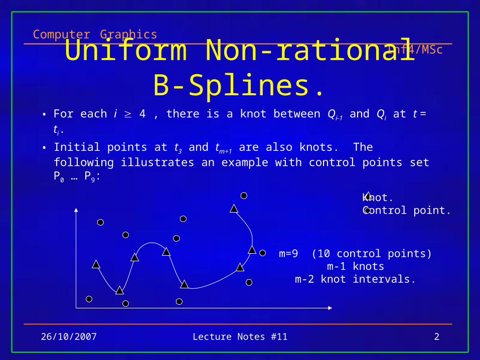
• For each i 4 , there is a knot between Qi-1 and Qi at t = ti.

• Initial points at t3 and tm+1 are also knots. The following illustrates an example with control points set P0 … P9:

Knot.Control point.

m=9 (10 control points)m-1 knots

m-2 knot intervals.




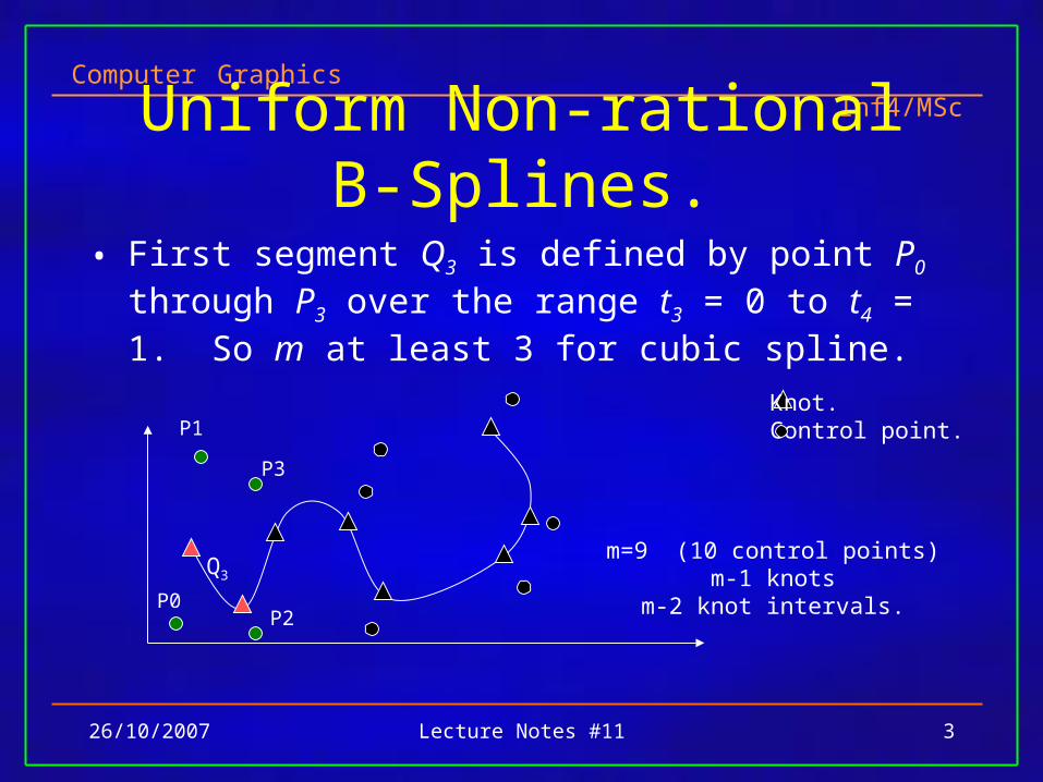
• First segment Q3 is defined by point P0 through P3 over the range t3 = 0 to t4 = 1. So m at least 3 for cubic spline.

Knot.Control point.P1

P2

P3

P0

Q3


m-2 knot intervals.




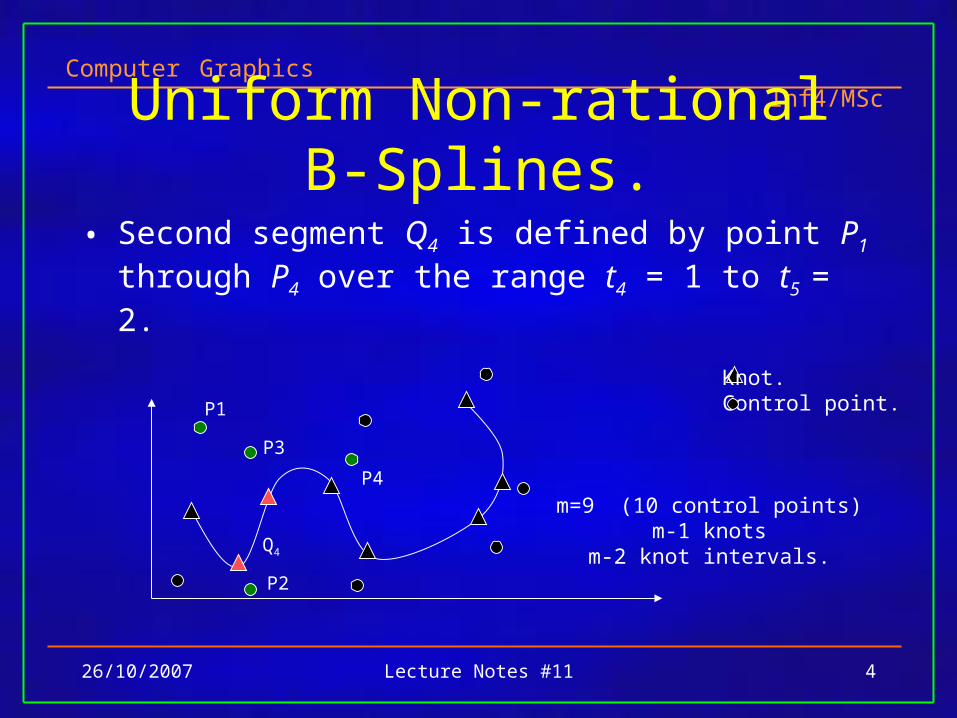
• Second segment Q4 is defined by point P1 through P4 over the range t4 = 1 to t5 = 2.

Knot.Control point.

Q4

P1

P3

P4

P2


m-2 knot intervals.



Uniform Non-Rational B-Splines

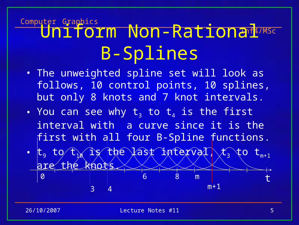
• The unweighted spline set will look as follows, 10 control points, 10 splines, but only 8 knots and 7 knot intervals.

• You can see why t3 to t4 is the first interval with a curve since it is the first with all four B-Spline functions.

• t9 to t10 is the last interval, t3 to tm+1 are the knots.

43t86 m

m+10



Cubic B-Splines

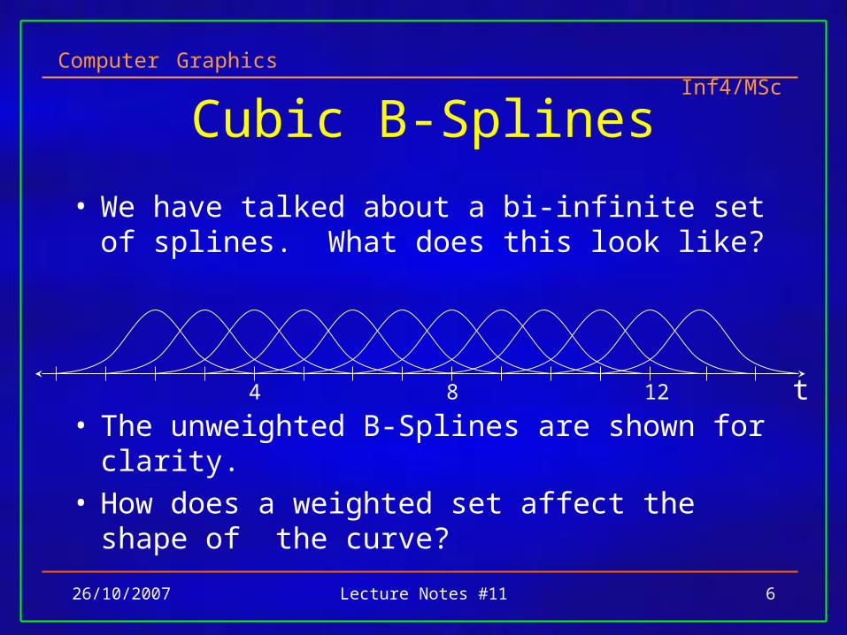
• We have talked about a bi-infinite set of splines. What does this look like?

• The unweighted B-Splines are shown for clarity.• How does a weighted set affect the shape of the

curve?

t4 8 12



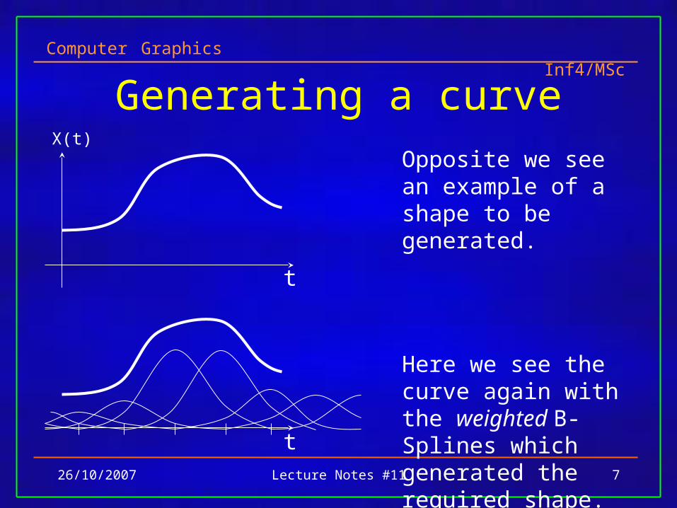
Generating a curveX(t)

t

t

Opposite we see an example of a shape to be generated.

Here we see the curve again with the weighted B-Splines which generated the required shape.



B-Spline example

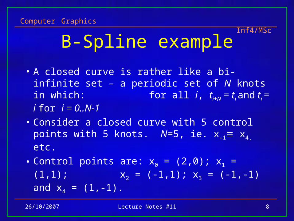
• A closed curve is rather like a bi-infinite set – a periodic set of N knots in which: for all i, ti+N = ti and ti = i for i = 0..N-1

• Consider a closed curve with 5 control points with 5 knots. N=5, ie. x–1 x4, etc.

• Control points are: x0 = (2,0); x1 = (1,1); x2 = (-1,1); x3 = (-1,-1) and x4 = (1,-1).



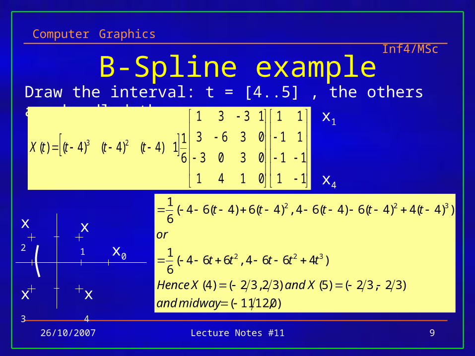
B-Spline exampleDraw the interval: t = [4..5] , the others are handled the same way.

11

11

11

11

0141

0303

0363

1331

6

11)4()4()4()( 23 ttttX

)0,1211(

)32,32()5()32,32()4(

)4664,664(6

1

))4(4)4(6)4(64,)4(6)4(64(6

1

322

322

midwayand

XandXHence

ttttt

or

ttttt

x0

x1x2

x3 x4

x4

x1


26/10/2007 Lecture Notes #11 10

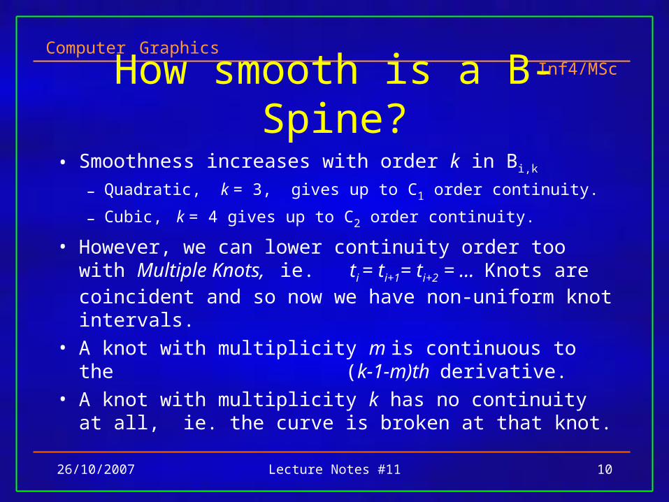
How smooth is a B-Spine?

• Smoothness increases with order k in Bi,k

– Quadratic, k = 3, gives up to C1 order continuity.

– Cubic, k = 4 gives up to C2 order continuity.

• However, we can lower continuity order too with Multiple Knots, ie. ti = ti+1= ti+2 = … Knots are coincident and so now we have non-uniform knot intervals.

• A knot with multiplicity m is continuous to the (k-1-m)th derivative.

• A knot with multiplicity k has no continuity at all, ie. the curve is broken at that knot.


26/10/2007 Lecture Notes #11 11

Non-Uniform Non-Rational B-Splines

• Note: as m increases by 1, an extra B-Spline function is attached to that knot: qiBi,k

• B-Splines have special forms at multiple knots.• Obtained from a recursive formula defining how

B-Splines are built, by setting m successive knots to be equal: tk+1 = tk+2 = … = tk+m

• No point in having m>k• Thus for endpoints to be on curve, they must have

a multiplicity of k, multiplicity of 4 in cubic case.


26/10/2007 Lecture Notes #11 12

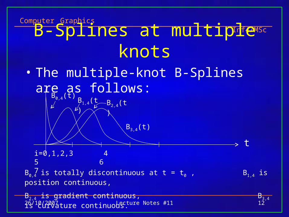
B-Splines at multiple knots

• The multiple-knot B-Splines are as follows:

t

B3,4(t)

B0,4(t) B1,4(t) B2,4(t)

i=0,1,2,3 4 5 6 7

B0,4 is totally discontinuous at t = t0 , B1,4 is position continuous,

B2,4 is gradient continuous, B3,4 is curvature continuous.


26/10/2007 Lecture Notes #11 13

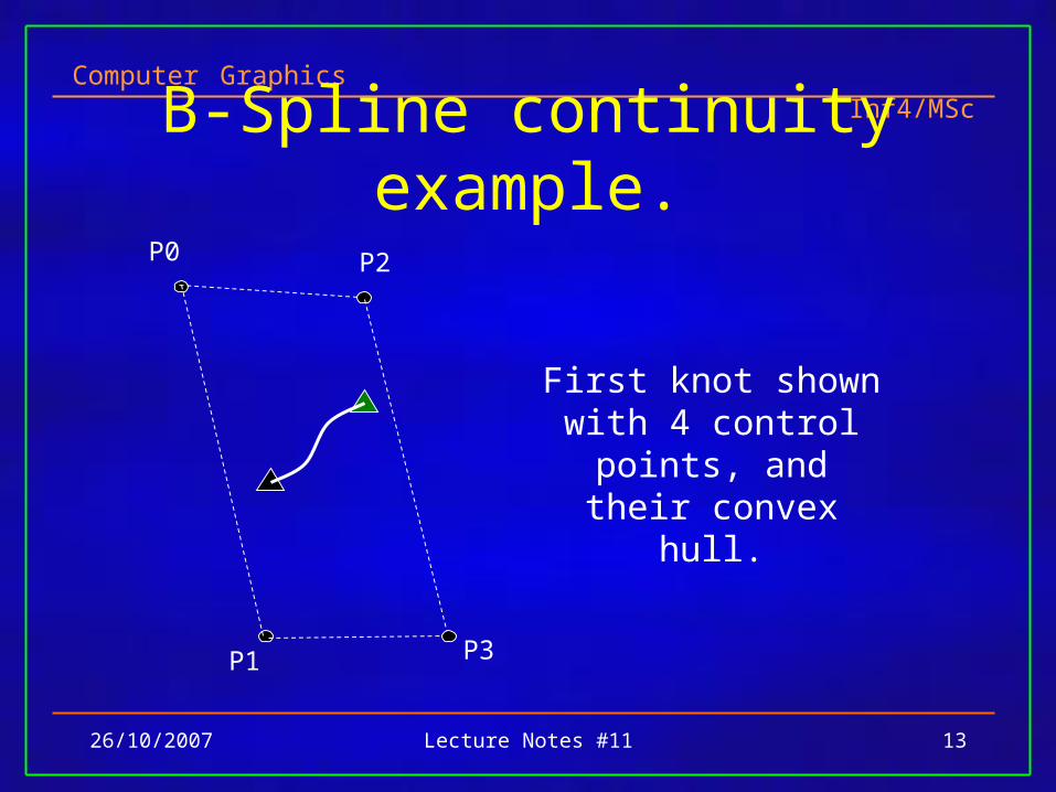
B-Spline continuity example.

First knot shown with 4 control points, and their

convex hull.

P1

P2P0

P3


26/10/2007 Lecture Notes #11 14

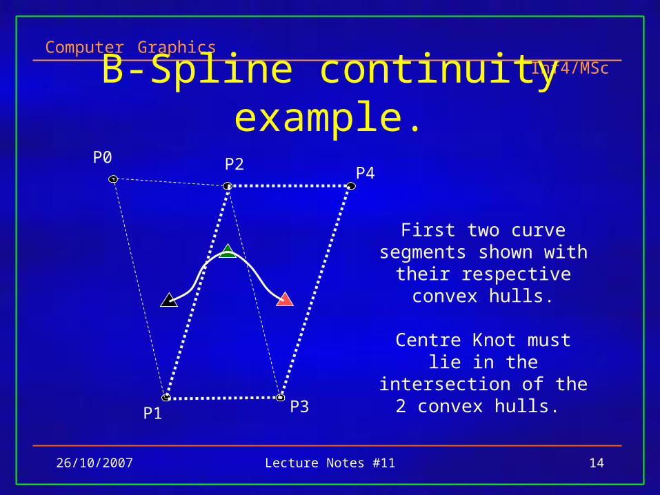
B-Spline continuity example.

First two curve segments shown with their respective

convex hulls.

Centre Knot must lie in the intersection of the 2 convex

hulls.

P1

P2P0P4

P3


26/10/2007 Lecture Notes #11 15

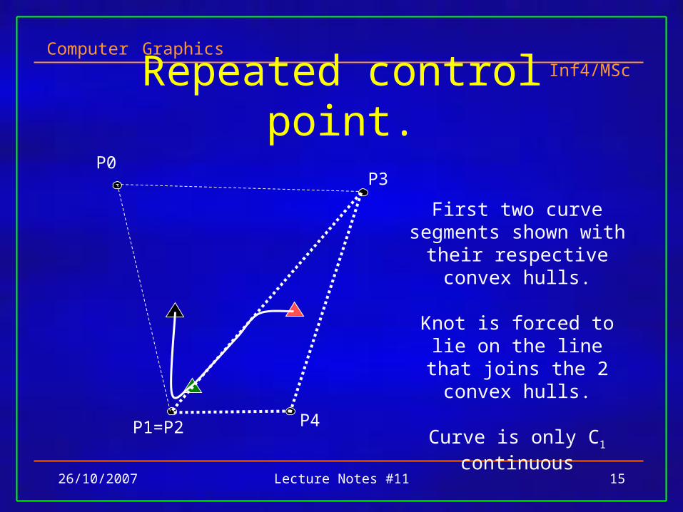
Repeated control point.

First two curve segments shown with their respective

convex hulls.

Knot is forced to lie on the line that joins the 2 convex

hulls.

Curve is only C1 continuous

P1=P2

P0P3

P4


26/10/2007 Lecture Notes #11 16

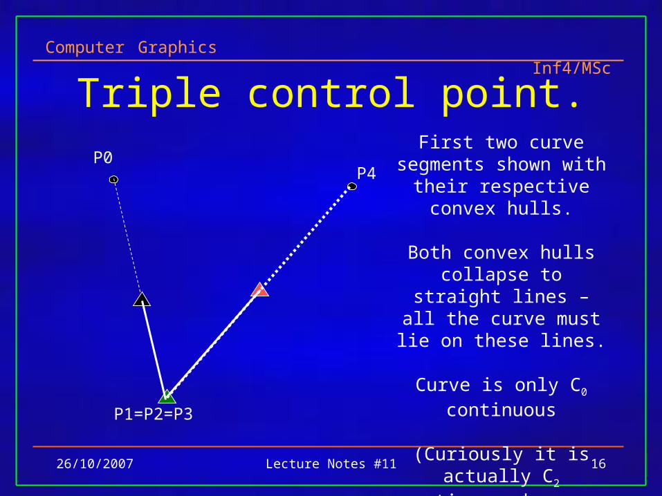
Triple control point.First two curve segments

shown with their respective convex hulls.

Both convex hulls collapse to straight lines – all the

curve must lie on these lines.

Curve is only C0 continuous

(Curiously it is actually C2 continuous because tangent

vector magnitude falls to zero at join. )

P1=P2=P3

P0P4


26/10/2007 Lecture Notes #11 17

Non-uniform non-rational B-splines.

• Parametric interval between knots does not have to be equal.

• Blending functions no longer the same for each interval.• Multiple knots may have to be spaced apart.• Advantages

– Continuity at selected control points can be reduced to C1 or lower – allows us to interpolate a control point without side-effects.

– Can interpolate start and end points. – Easy to add extra knots and control points.


26/10/2007 Lecture Notes #11 18

Summary of B-Splines.• Functions that can interpolate a series of control points with C2

continuity and local control.• Don’t pass through their control points, although can be forced.

– note that if an order k B-Spline has k points locally colinear then a straight-line section will result midway in the set, and will touch (tangentially) the convex hull for (k – 1) colinear control points.

• Uniform– Knots are equally spaced in t.

• Non-Uniform– Knots are unequally spaced– Allows addition of extra control points anywhere in the set.


26/10/2007 Lecture Notes #11 19

Summary cont.• For interactive curve modelling

– B-Splines are very good.

• To interpolate a number of positions – Catmull-Rom splines are best.

• To interpolate with tangent control– Hemite or Bézier forms are useful and most often used.

• To draw a spline.– Brute force method : Evaluate matrix to get parametric expressions

for coordinates. Then for small increments of t, join with line segments.

– Better : use method of forward differences to express spline in t form.


26/10/2007 Lecture Notes #11 20

Surfaces – a simple extension

• Easy to generalise from cubic curves to bicubic surfaces.

• Surfaces defined by parametric equations of two variables, s and t.

• ie. a surface is approximated by a series of crossing parametric cubic curves

• Result is a polygon mesh and decreasing step size in s and t will give a mesh of small near-planar quadrilateral patches and more accuracy.

1010 tands


26/10/2007 Lecture Notes #11 21

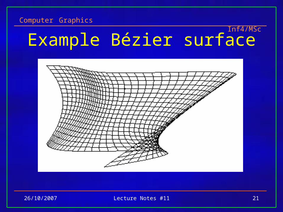
Example Bézier surface


26/10/2007 Lecture Notes #11 22

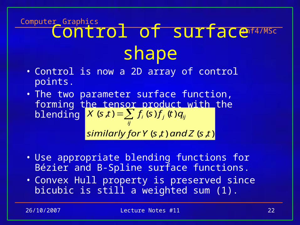
Control of surface shape

• Control is now a 2D array of control points.• The two parameter surface function, forming the

tensor product with the blending functions is:

• Use appropriate blending functions for Bézier and B-Spline surface functions.

• Convex Hull property is preserved since bicubic is still a weighted sum (1).

),(),(

)()(),(

tsZandtsYforsimilarly

qtfsftsX ijjij

i


26/10/2007 Lecture Notes #11 23

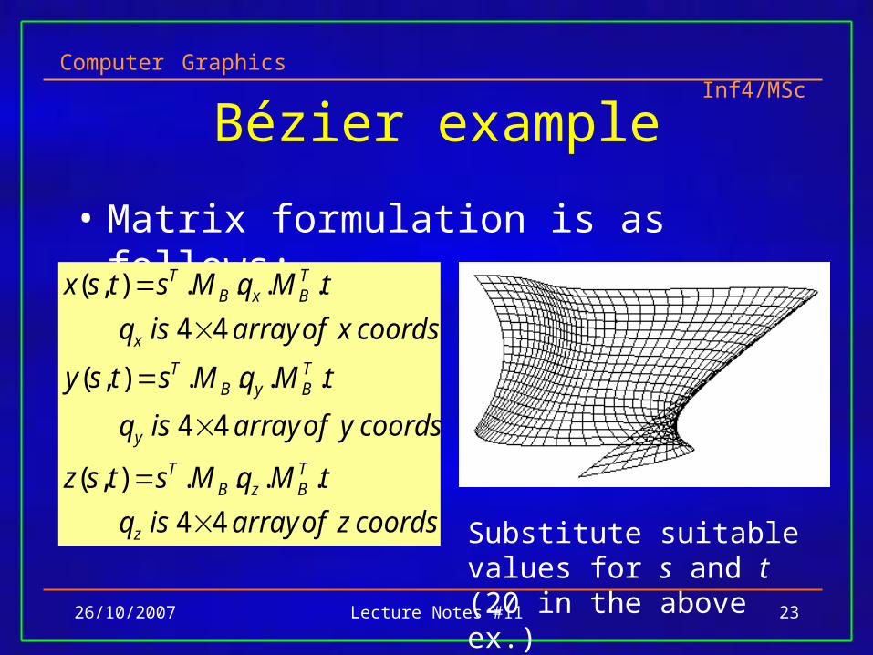
Bézier example

• Matrix formulation is as follows:

coordszofarrayisq

tMqMstsz

coordsyofarrayisq

tMqMstsy

coordsxofarrayisq

tMqMstsx

z

TBzB

T

y

TByB

T

x

TBxB

T

44

....),(

44

....),(

44

....),(

Substitute suitable values for s and t (20 in the above ex.)


26/10/2007 Lecture Notes #11 24

B-Spline surfaces• Break surface into 4-sided patches choosing

suitable values for s and t.• Points on any external edges must be multiple

knots of multiplicity k.• Lot more work than Bézier.• There are other types of spline systems and

NURBS modelling packages are available to make the work much easier.

• Use polygon packages for display, hidden-surface removal and rendering. (Bézier too)


26/10/2007 Lecture Notes #11 25

Continuity of Bicubic patches.

• Hermite and Bézier patches– C0 continuity by sharing 4 control points

between patches.

– C1 continuity when both sets of control points either side of the edge are collinear with the edge.

• B-Spline patch.– C2 continuity between patches.


26/10/2007 Lecture Notes #11 26

Displaying Bicubic patches.

• Can calculate surface normals to bicubic surfaces by vector cross product of the 2 tangent vectors.

• Normal is expensive to compute– Formulation of normal is a biquintic (two-

variable,fifth-degree) polynomial.

• Display.– Can use brute-force method – very expensive !

– Forward differencing method very attractive.


26/10/2007 Lecture Notes #11 27

Reading for this lecture

• Foley at al., Chapter 11, sections 11.2.3, 11.2.4, 11.2.9, 11.2.10, 11.3 and 11.5.

• Introductory text, Chapter 9, sections 9.2.4, 9.2.5, 9.2.7, 9.2.8 and 9.3.

• Other texts: look for B-Splines UNRBS, NUNRBS, something on forward difference method, comparison of systems, and Bézier and B-Spline surface modelling.

Documents

Computer Graphics Inf4/MSc Computer Graphics Lecture Notes #11 Curves and Surfaces II