Embed Size (px)
Citation preview
Computer Graphics Inf4/MSc
Computer Graphics
Lecture 10
Curves and Surfaces
I
Computer Graphics Inf4/MSc
23/10/2007 Lecture 10 2
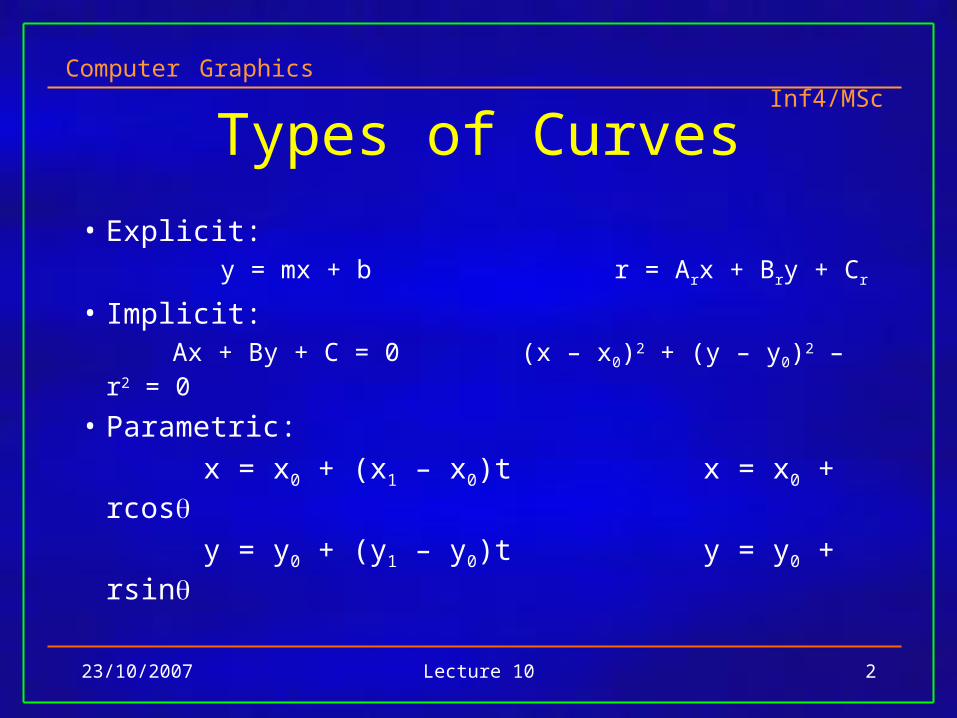
Types of Curves
• Explicit: y = mx + b r = Arx + Bry + Cr
• Implicit: Ax + By + C = 0 (x – x0)2 + (y – y0)2 – r2 = 0
• Parametric:
x = x0 + (x1 – x0)t x = x0 + rcos
y = y0 + (y1 – y0)t y = y0 + rsin
Computer Graphics Inf4/MSc
23/10/2007 Lecture 10 3
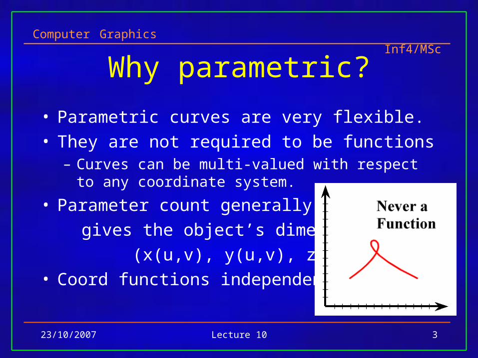
Why parametric?
• Parametric curves are very flexible.• They are not required to be functions
– Curves can be multi-valued with respect to any coordinate system.
• Parameter count generally
gives the object’s dimension.
(x(u,v), y(u,v), z(u,v))• Coord functions independent.
Computer Graphics Inf4/MSc
23/10/2007 Lecture 10 4
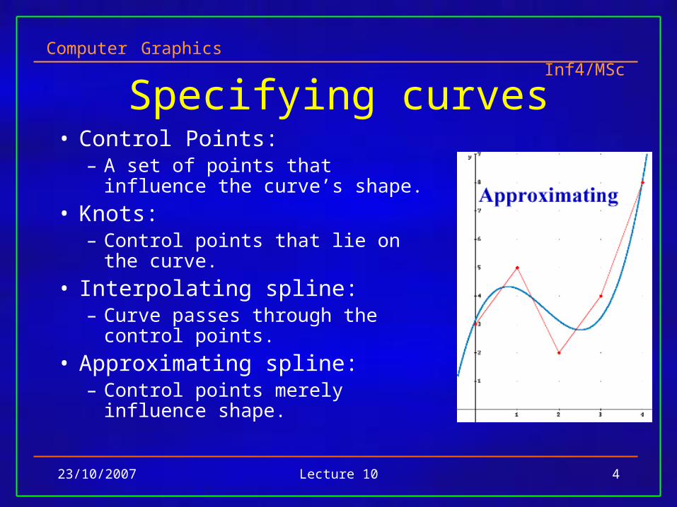
Specifying curves• Control Points:
– A set of points that influence the curve’s shape.
• Knots:– Control points that lie on the curve.
• Interpolating spline:– Curve passes through the control
points.
• Approximating spline:– Control points merely influence
shape.
Computer Graphics Inf4/MSc
23/10/2007 Lecture 10 5
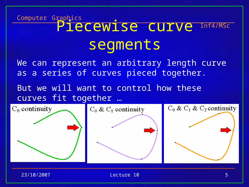
Piecewise curve segments
We can represent an arbitrary length curve as a series of curves pieced together.
But we will want to control how these curves fit together …
Computer Graphics Inf4/MSc
23/10/2007 Lecture 10 6
Parametric Cubic Curves
• In order to assure C2 continuity our functions must be of at least degree 3. This is also the lowest order to describe a non-planar curve.
• Cubic has 4 degrees of freedom and can control 4 things.
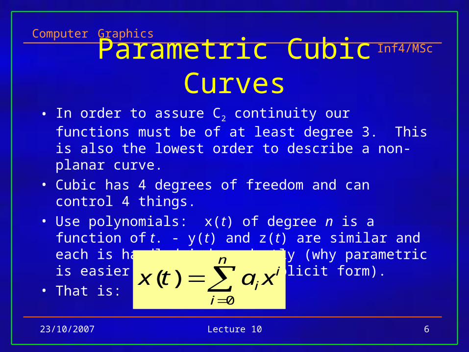
• Use polynomials: x(t) of degree n is a function of t. - y(t) and z(t) are similar and each is handled independently (why parametric is easier to handle than implicit form).
• That is: i
n
ii xatx
0
)(
Computer Graphics Inf4/MSc
23/10/2007 Lecture 10 7
An Illustrative Example
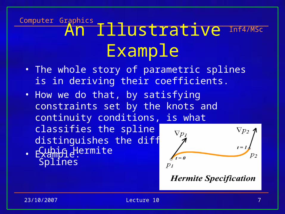
• The whole story of parametric splines is in deriving their coefficients.
• How we do that, by satisfying constraints set by the knots and continuity conditions, is what classifies the spline system and distinguishes the different systems.
• Example:
Cubic Hermite Splines
Computer Graphics Inf4/MSc
23/10/2007 Lecture 10 8
Hermite splines
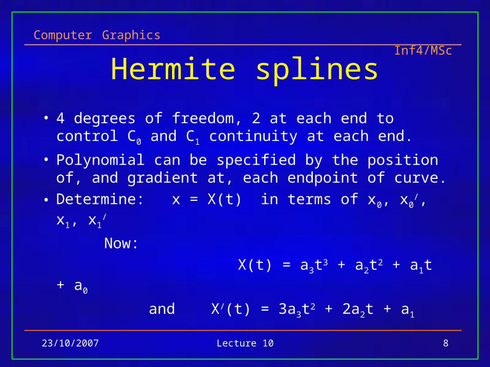
• 4 degrees of freedom, 2 at each end to control C0 and C1 continuity at each end.
• Polynomial can be specified by the position of, and gradient at, each endpoint of curve.
• Determine: x = X(t) in terms of x0, x0/, x1, x1
/
Now:
X(t) = a3t3 + a2t2 + a1t + a0
and X/(t) = 3a3t2 + 2a2t + a1
Computer Graphics Inf4/MSc
23/10/2007 Lecture 10 9
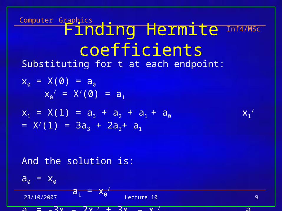
Finding Hermite coefficientsSubstituting for t at each endpoint:
x0 = X(0) = a0 x0/ = X/(0) = a1
x1 = X(1) = a3 + a2 + a1 + a0 x1/ = X/(1) = 3a3 + 2a2+ a1
And the solution is:
a0 = x0 a1 = x0/
a2 = -3x0 – 2x0/ + 3x1 – x1
/ a3 = 2x0 + x0/ - 2x1 + x1
/
Computer Graphics Inf4/MSc
23/10/2007 Lecture 10 10
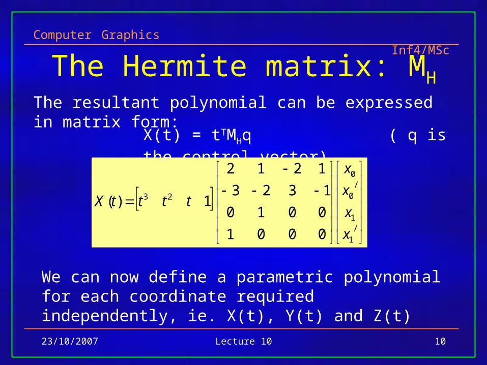
The Hermite matrix: MH
The resultant polynomial can be expressed in matrix form:
X(t) = tTMHq ( q is the control vector)
/1
1
/0
0
23
0001
0010
1323
1212
1)(
x
x
x
x
ttttX
We can now define a parametric polynomial for each coordinate required independently, ie. X(t), Y(t) and Z(t)
Computer Graphics Inf4/MSc
23/10/2007 Lecture 10 11
Hermite Basis (Blending) Functions
x0 x1
x0/
x1/
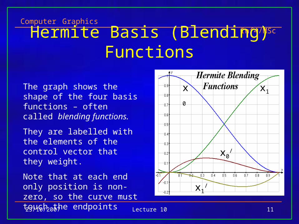
The graph shows the shape of the four basis functions – often called blending functions.
They are labelled with the elements of the control vector that they weight.
Note that at each end only position is non-zero, so the curve must touch the endpoints
Computer Graphics Inf4/MSc
23/10/2007 Lecture 10 12
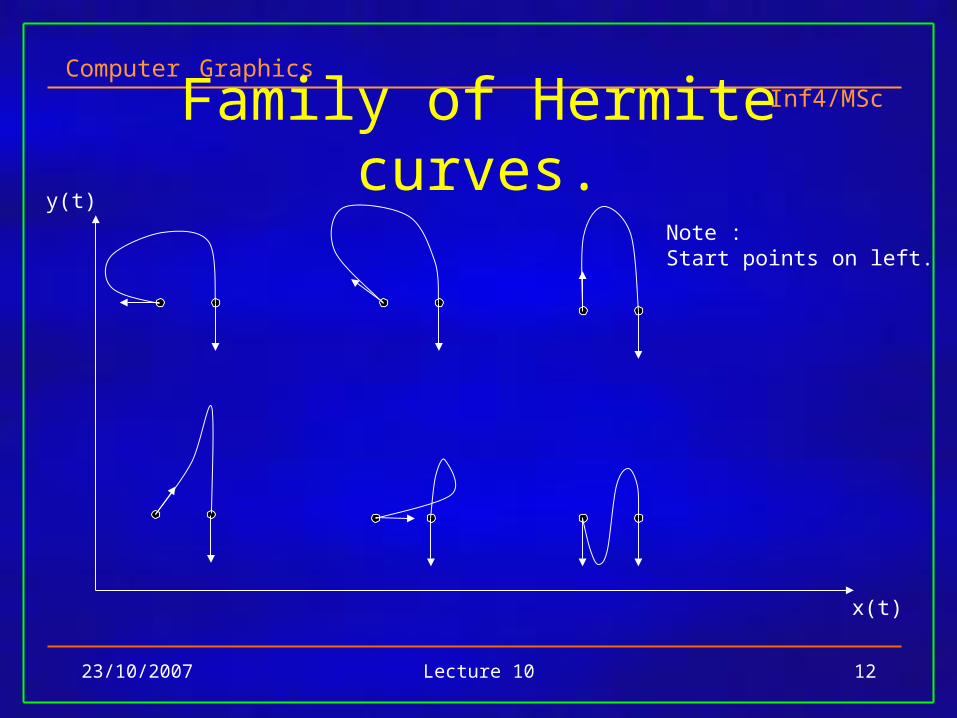
Family of Hermite curves.
x(t)
y(t)
Note : Start points on left.
Computer Graphics Inf4/MSc
23/10/2007 Lecture 10 13
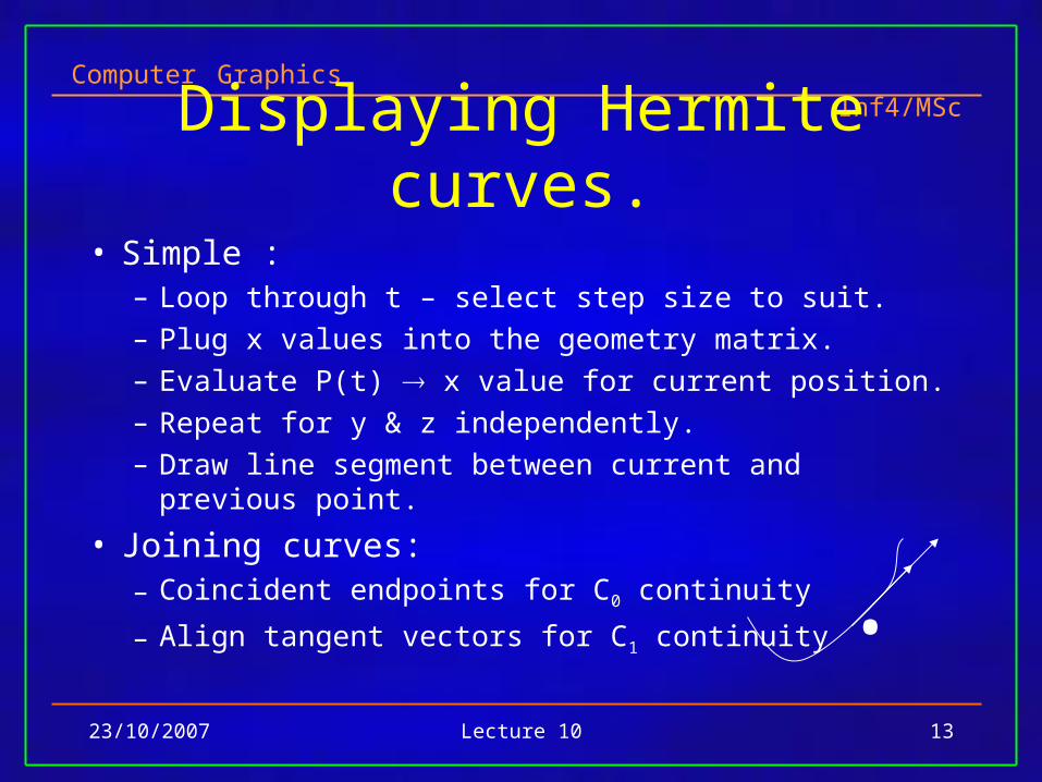
Displaying Hermite curves.
• Simple : – Loop through t – select step size to suit.
– Plug x values into the geometry matrix.
– Evaluate P(t) x value for current position.
– Repeat for y & z independently.
– Draw line segment between current and previous point.
• Joining curves:– Coincident endpoints for C0 continuity
– Align tangent vectors for C1 continuity
.
Computer Graphics Inf4/MSc
23/10/2007 Lecture 10 14
Bézier Curves
• Hermite cubic curves are difficult to model – need to specify point and gradient.
• More intuitive to only specify points.• Pierre Bézier specified 2 endpoints and 2
additional control points to specify the gradient at the endpoints.
• Can be derived from Hermite matrix:– Two end control points specify tangent
Computer Graphics Inf4/MSc
23/10/2007 Lecture 10 15
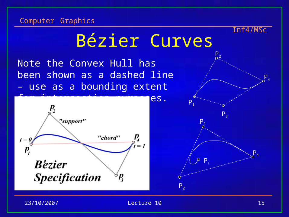
Bézier Curves
P2
P1
P4
P3
P3
P4
P2
P1
Note the Convex Hull has been shown as a dashed line – use as a bounding extent for intersection purposes.
Computer Graphics Inf4/MSc
23/10/2007 Lecture 10 16
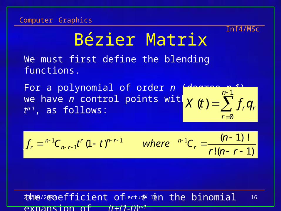
Bézier MatrixWe must first define the blending functions.
For a polynomial of order n (degree n-1), we have n control points with terms up to tn-1, as follows:
fr is a blending function
the coefficient of tr in the binomial expansion of (t+(1-t))n-1
r
n
rrqftX
1
0
)(
)!1(!
)!1()1( 11
11
rnr
nCwherettCf r
nrnrrn
nr
Computer Graphics Inf4/MSc
23/10/2007 Lecture 10 17
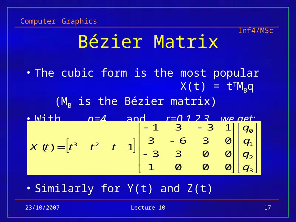
Bézier Matrix
• The cubic form is the most popular X(t) = tTMBq (MB is the Bézier matrix)
• With n=4 and r=0,1,2,3 we get:
• Similarly for Y(t) and Z(t)
3
2
1
0
23
0001
0033
0363
1331
1)(
q
q
q
q
ttttX
Computer Graphics Inf4/MSc
23/10/2007 Lecture 10 18
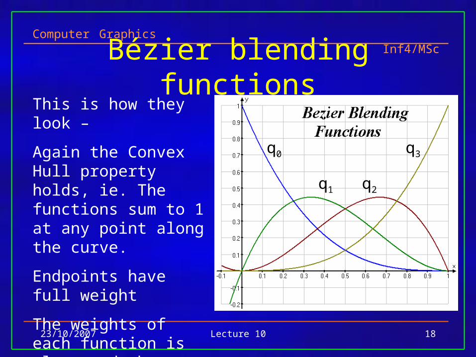
Bézier blending functionsThis is how they look –
Again the Convex Hull property holds, ie. The functions sum to 1 at any point along the curve.
Endpoints have full weight
The weights of each function is clear and the labels show the control points being weighted.
q0 q3
q1 q2
Computer Graphics Inf4/MSc
23/10/2007 Lecture 10 19
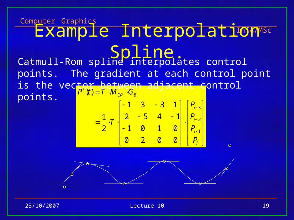
Example Interpolation Spline.
i
i
i
i
BCRi
P
P
P
P
T
GMTtP
1
2
3
0020
0101
1452
1331
2
1
)(
Catmull-Rom spline interpolates control points. The gradient at each control point is the vector between adjacent control points.
Computer Graphics Inf4/MSc
23/10/2007 Lecture 10 20
Uniform Nonrational B-Splines
• Cubic Bézier curves are joined together in the same way as Hermite curves for arbitrary length by joining short 4-point pieces with C0 and C1 order continuity.
• However cubic B-Splines can have any number of control points and any length of curve with C0, C1 and C2 order continuity.
• Segments of the B-Spline, joined at knots, depend on a few adjacent control points which are shared between segments for continuity.
Computer Graphics Inf4/MSc
23/10/2007 Lecture 10 21
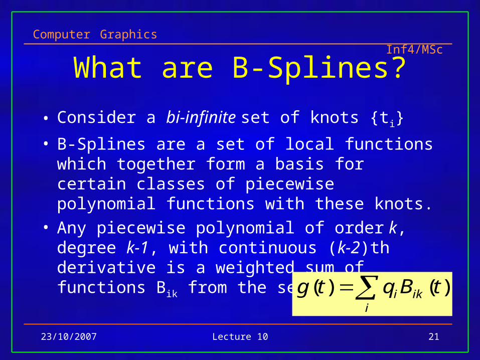
What are B-Splines?
• Consider a bi-infinite set of knots {ti}
• B-Splines are a set of local functions which together form a basis for certain classes of piecewise polynomial functions with these knots.
• Any piecewise polynomial of order k, degree k-1, with continuous (k-2)th derivative is a weighted sum of functions Bik from the set:
)()( tBqtg iki
i
Computer Graphics Inf4/MSc
23/10/2007 Lecture 10 22
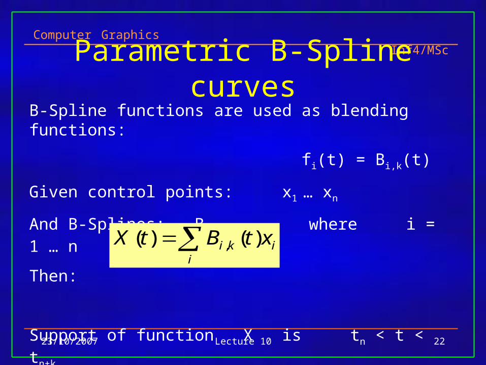
Parametric B-Spline curvesB-Spline functions are used as blending functions:
fi(t) = Bi,k(t)
Given control points: x1 … xn
And B-Splines: Bi,k where i = 1 … n
Then:
Support of function X is tn < t < tn+k
ie. the range over which X is non-zero.
ii
ki xtBtX )()( ,
Computer Graphics Inf4/MSc
23/10/2007 Lecture 10 23
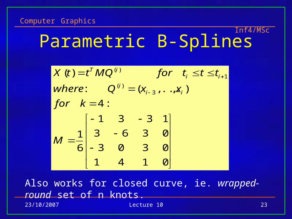
Parametric B-Splines
0141
0303
0363
1331
6
1
:4
),...,(:
)(
3)(
1)(
M
kfor
xxQwhere
tttforMQttX
iii
iiiT
Also works for closed curve, ie. wrapped-round set of n knots.
Computer Graphics Inf4/MSc
23/10/2007 Lecture 10 24
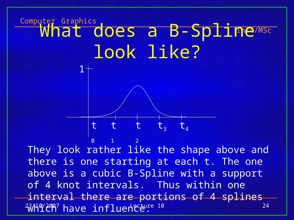
What does a B-Spline look like?
t0 t1 t2 t3 t4
1
They look rather like the shape above and there is one starting at each t. The one above is a cubic B-Spline with a support of 4 knot intervals. Thus within one interval there are portions of 4 splines which have influence.
Computer Graphics Inf4/MSc
23/10/2007 Lecture 10 25
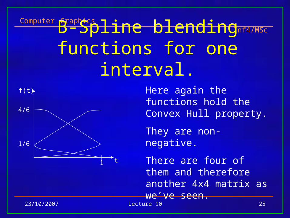
B-Spline blending functions for one interval.
t1
1/6
4/6
f(t) Here again the functions hold the Convex Hull property.
They are non-negative.
There are four of them and therefore another 4x4 matrix as we’ve seen.
Computer Graphics Inf4/MSc
23/10/2007 Lecture 10 26
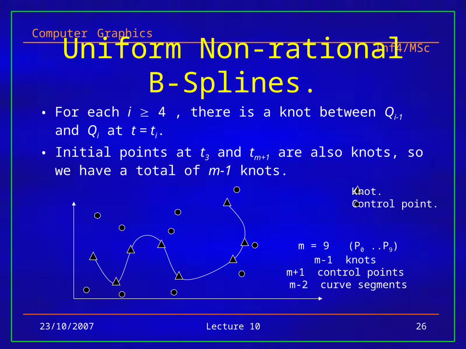
Uniform Non-rational B-Splines.
• For each i 4 , there is a knot between Qi-1 and Qi at t = ti.
• Initial points at t3 and tm+1 are also knots, so we have a total of m-1 knots.
Knot.Control point.
m = 9 (P0 ..P9)m-1 knots
m+1 control points m-2 curve segments
Computer Graphics Inf4/MSc
23/10/2007 Lecture 10 27
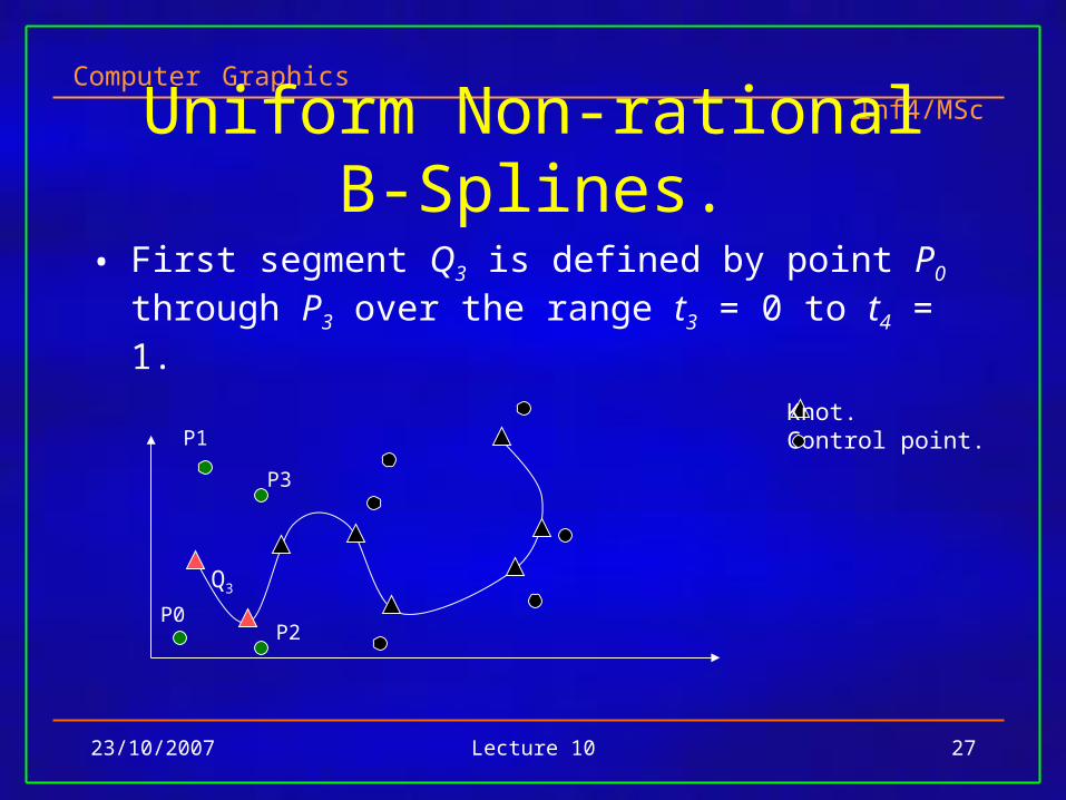
Uniform Non-rational B-Splines.
• First segment Q3 is defined by point P0 through P3 over the range t3 = 0 to t4 = 1.
Knot.Control point.P1
P2
P3
P0
Q3
Computer Graphics Inf4/MSc
23/10/2007 Lecture 10 28
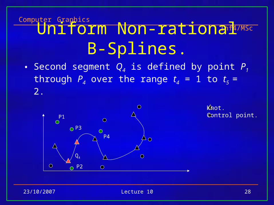
Uniform Non-rational B-Splines.
• Second segment Q4 is defined by point P1 through P4 over the range t4 = 1 to t5 = 2.
Knot.Control point.
Q4
P1
P3
P4
P2
Computer Graphics Inf4/MSc
23/10/2007 Lecture 10 29
Reading for this lecture
• Foley et al. Chapter 11, section 11.2 up to and including 11.2.3
• Introductory text Chapter 9, section 9.2 up to and including section 9.2.4