Modeling and Simulating Flow Phenomenon using Navier

Proceedings of the International Conference on Industrial Engineering and Operations Management

Rabat, Morocco, April 11-13, 2017

1902

Modeling and Simulating Flow Phenomenon using

Navier-Stokes Equation

Hyunjun Min, Jiho Shin, Jaeho Choi, and Hohyun Lee

Data Science Lab, Paul Math School 12-11, Dowontongmi-gil, Cheongcheon-myeon, Goesan County, Republic of Korea

[email protected], [email protected], [email protected], [email protected]

Abstract

Due to drastic development in computing environment Computational Fluid Dynamics (CFD) area can be simply modeled and simulated for better understanding of complex systems. So it enables many analysis of complex flux. In this research induce Navier-Stokes equation’s mathematical, Fluid dynamical content and examine using method in CFD and compared result of CFD and result of coding. lastly induce governed equation at model’s conditions.

Keywords

Computational fluid dynamics, Navier-Stokes Eq., Flow phenomenon, Fluid dynamics

1. Introduction

Navier-Stokes Equation is governing equation of Flu id dynamics and used importantly on many areas like

Mechanical engineering, Mathematics , Flu id dynamics, civil engineering. In this equation’s case can signify perfect

flow because it gets variables about all of value which is about fluid flow. So this equation always imp ortantly come

to the fore on Fluid dynamics. But Navier-Stokes equation get variable about all of value, so find 3-D Navier-Stokes

equation solution problem is reg istration on Millennium problem by Clay Mathematics Institute (CMI). In beginning

Navier-Stokes equation be promising to peoples because of possibility to calculate every fluid flow academically.

But in reality applicable models are only few. Now due to development of computer, copious calculat ion (human

impossible to calculate) enable to calcu late. So acceptable model’s area increase and now pioneer to Medical science

area like analysis of vascular flow.

Cholesterol which ingest with nourishment adhere to b lood vessel wall and caused many adult diseases like

Myocardial infarction and Atherosclerosis. Cholesterol grow vertically due to Cholesterol reduce area.

According to Bermouilli equation, area and velocity are d irect proportion. So If cholesterol adhere to blood vessel

wall, area become s maller than normal blood vessel’s cross -section area and then velocity become faster. Due to fast

velocity, Cholesterol’s edge gets hurt. So scab created on the cholesterol and area become smaller than before.

Cholesterol widely and constantly increase due to the blood retention which caused by the gap created by

cholesterols and blood vessel wall at the backside of the cholesterols.

We started this study to analysis about various flow phenomenon with Navier-Stokes equation on the fluid

dynamical viewpoint and analysis formula on the mathematical viewpoint in this situation.

In this paper analysis Navier-Stokes equation which simplify basic blood flow to modeling similar to cholesterol

interrupter at the blood vessel wall. And we run CFD with correct condition. After that we compare analysis value

which analysis by Navier-Stokes equation, CFD and cording (use programing language C). And this is the final

purpose and conclusion of this research.



1903

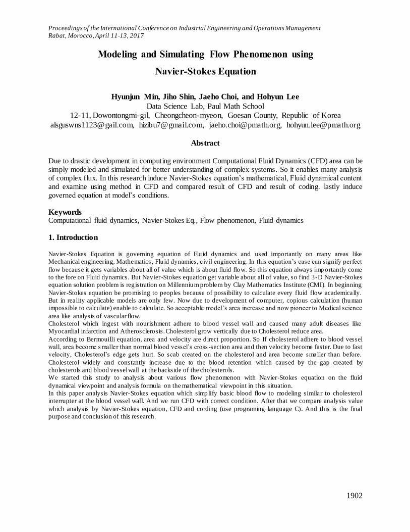
Fig 1 Study method

2. Body

2.1 Precedence study for blood flow analysis

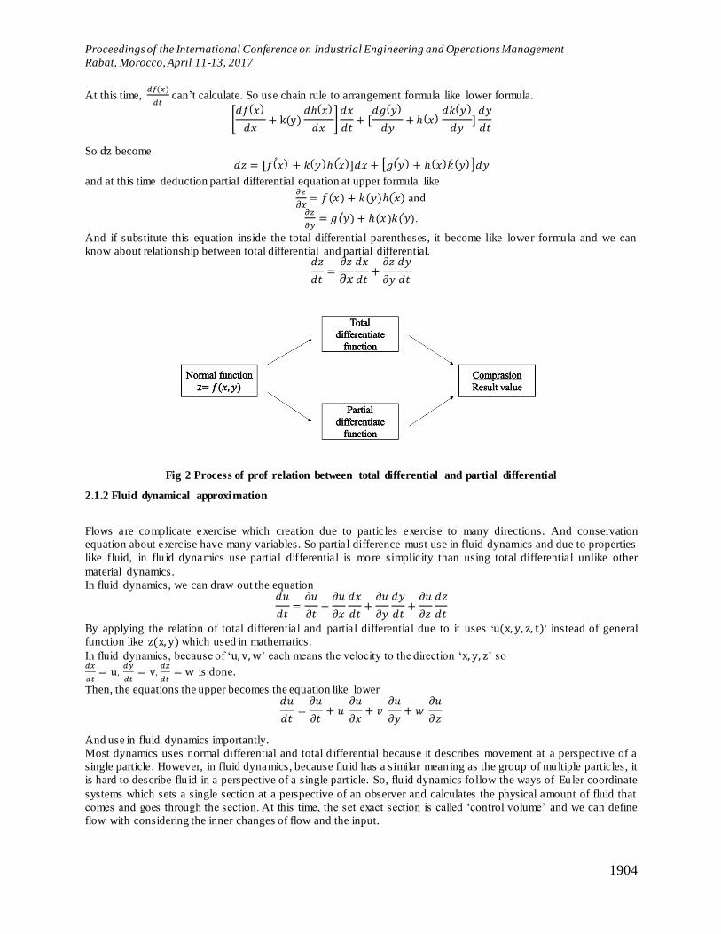
2.1.1 Total differential and partial differential

Lower formula is very important in fluid dynamics. 𝑑𝑢

𝑑𝑡=

𝜕𝑢

𝜕𝑡+ 𝑢

𝜕𝑢

𝜕𝑥+ 𝑣

𝜕𝑢

𝜕𝑦+ 𝑤

𝜕𝑢

𝜕𝑧

Like this formula is directed by process of proof relationship between total differential and partial differential

mathematically.

Total differential and part ial differential is differential of h igher than two variable function like z = f(x, y). So it is

differential of type of function which has many variables. If analysis relat ionship mathematically, normal function

z = f(x, y) is formula which made up with x, y. So z = f(x, y) can transformation like

F(x, y) = formula about x + formula about y + (formula about x)(formula about y)

So z = f(x, y) change like lower. 𝑧 = 𝐹(𝑥,𝑦) = 𝑓(𝑥) + 𝑔(𝑦) + ℎ(𝑥)𝑘(𝑦)

At this time conduct partial differential to get 𝜕𝑧

𝜕𝑥 is like lower formula.

𝜕𝑧

𝜕𝑥=

𝜕𝑓(𝑥)

𝜕𝑥+

𝜕𝑔(𝑦)

𝜕𝑥+

𝜕ℎ(𝑥)𝑘(𝑦)

𝜕𝑥

At this point 𝜕𝑧

𝜕𝑥 is partial differential about x, so if calcu late partial differential, y treated like constant number. So

equation like lower came out. 𝜕𝑧

𝜕𝑥=

𝜕𝑓(𝑥)

𝜕𝑥+ 𝑘(𝑦)

𝜕ℎ (𝑥)

𝜕𝑥

And then upper formula become like lower formula 𝜕𝑧

𝜕𝑥= 𝑓(𝑥)́ + k(y)ℎ(𝑥)́

and sameness, 𝜕𝑧

𝜕𝑦 become like lower formula

𝜕𝑧

𝜕𝑦= 𝑔(𝑦)́ + ℎ(𝑥)𝑘(𝑦)́

Next is arrange method use total differential.

Different with upper formula, this formula differential totally. So if z is z = f(x, y) , 𝑑𝑧

𝑑𝑡 is developed like lower

formula. 𝑑𝑧

𝑑𝑡=

𝑑𝑓(𝑥)

𝑑𝑡+

𝑑𝑔(𝑦)

𝑑𝑡+ k(y)

𝑑ℎ(𝑥)

𝑑𝑡+ ℎ(𝑥)

𝑑𝑘(ℎ)

𝑑𝑡



1904

At this time, 𝑑𝑓(𝑥)

𝑑𝑡 can’t calculate. So use chain rule to arrangement formula like lower formula.

[𝑑𝑓(𝑥)

𝑑𝑥+ k(y)

𝑑ℎ(𝑥)

𝑑𝑥]

𝑑𝑥

𝑑𝑡+ [

𝑑𝑔(𝑦)

𝑑𝑦+ ℎ(𝑥)

𝑑𝑘(𝑦)

𝑑𝑦]

𝑑𝑦

𝑑𝑡

So dz become

𝑑𝑧 = [𝑓(𝑥)́ + 𝑘(𝑦)ℎ(𝑥)́ ]𝑑𝑥 + [𝑔(𝑦)́ + ℎ(𝑥)�́�(𝑦) ]𝑑𝑦

and at this time deduction partial differential equation at upper formula like 𝜕𝑧

𝜕𝑥= 𝑓(𝑥)́ + 𝑘(𝑦)ℎ(𝑥)́ and

𝜕𝑧

𝜕𝑦= 𝑔(𝑦)́ + ℎ(𝑥)𝑘(𝑦)́ .

And if substitute this equation inside the total differential parentheses, it become like lower formula and we can

know about relationship between total differential and partial differential. 𝑑𝑧

𝑑𝑡=

𝜕𝑧

𝜕𝑥

𝑑𝑥

𝑑𝑡+

𝜕𝑧

𝜕𝑦

𝑑𝑦

𝑑𝑡

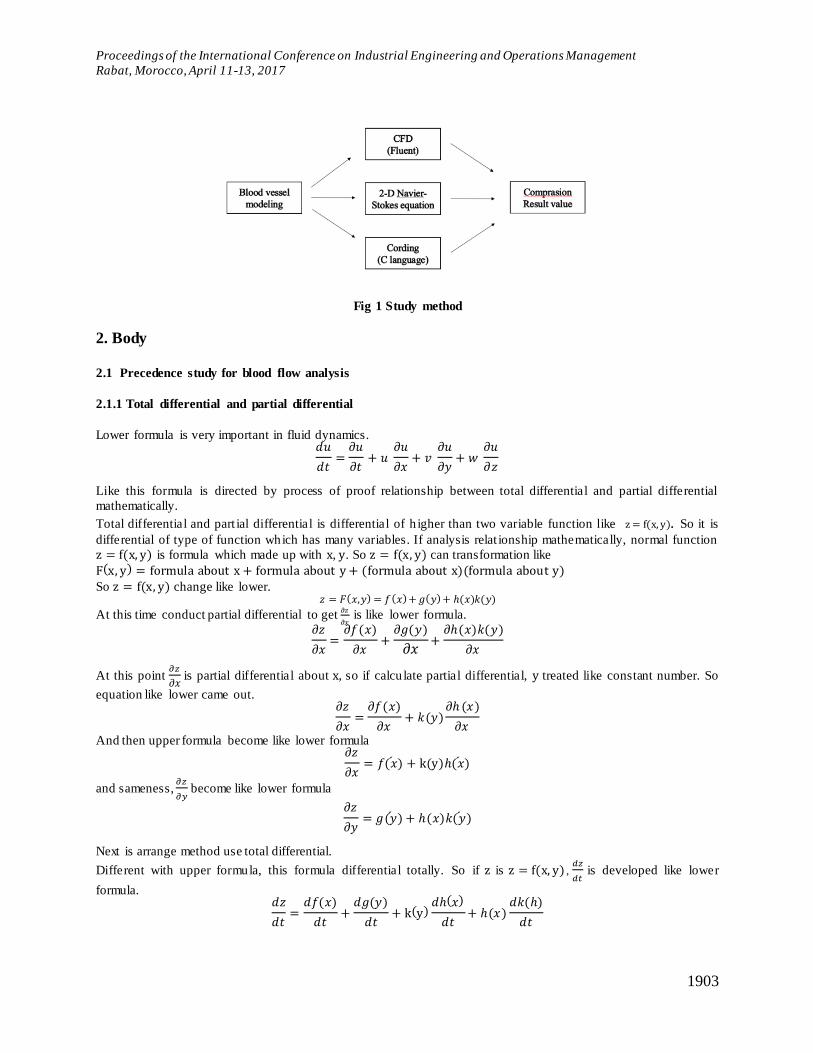
Fig 2 Process of prof relation between total differential and partial differential

2.1.2 Fluid dynamical approximation

Flows are complicate exercise which creation due to particles exercise to many directions. And conservation

equation about exercise have many variables. So partial difference must use in fluid dynamics and due to properties

like fluid, in flu id dynamics use partial differential is more simplicity than using total differential unlike other

material dynamics.

In fluid dynamics, we can draw out the equation 𝑑𝑢

𝑑𝑡=

𝜕𝑢

𝜕𝑡+

𝜕𝑢

𝜕𝑥

𝑑𝑥

𝑑𝑡+

𝜕𝑢

𝜕𝑦

𝑑𝑦

𝑑𝑡+

𝜕𝑢

𝜕𝑧

𝑑𝑧

𝑑𝑡

By applying the relation of total differential and partial differential due to it uses ‘u(x, y, z, t)’ instead of general

function like z(x, y) which used in mathematics.

In fluid dynamics, because of ‘u, v, w’ each means the velocity to the direction ‘x, y, z’ so 𝑑𝑥

𝑑𝑡= u,

𝑑𝑦

𝑑𝑡= v,

𝑑𝑧

𝑑𝑡= w is done.

Then, the equations the upper becomes the equation like lower 𝑑𝑢

𝑑𝑡=

𝜕𝑢

𝜕𝑡+ 𝑢

𝜕𝑢

𝜕𝑥+ 𝑣

𝜕𝑢

𝜕𝑦+ 𝑤

𝜕𝑢

𝜕𝑧

And use in fluid dynamics importantly.

Most dynamics uses normal differential and total d ifferential because it describes movement at a perspect ive of a

single particle. However, in fluid dynamics, because flu id has a similar meaning as the group of multiple particles, it

is hard to describe flu id in a perspective of a single part icle. So, flu id dynamics fo llow the ways of Eu ler coordinate

systems which sets a single section at a perspective of an observer and calculates the physical amount of fluid that

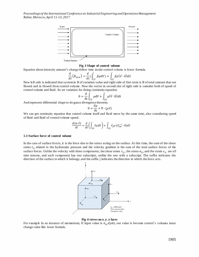
comes and goes through the section. At this time, the set exact section is called ‘control volume’ and we can define

flow with considering the inner changes of flow and the input.



1905

Fig 3 Shape of control volume

Equation about intensity amount’s change follow time inside control volume is lower formula.

𝑑

𝑑𝑡(𝐵𝑠𝑦𝑠𝑡 ) =

𝑑

𝑑𝑡(∫ 𝛽𝜌𝑑𝑉) + ∫ 𝛽𝜌(𝑣 ∙ �⃗⃗�)𝑑𝑆

𝐶𝑆𝐶𝑉

Now left side is indicated that system in B of variation value and right side of first term is B of total amount that out

flowed and in flowed from control volume. Now the vector in second slot of right side is consider both of speed of

control volume and fluid. So we variation for doing continuity equation.

0 =d

dt∫ ρdV + ∫ ρ(v⃗⃗ ∙ n⃗⃗)dS

CSCV

And represent differential shape to do gauss divergence theorem.

0 =∂ρ

∂t+ ∇ ∙ (𝜌𝑣)

We can get continuity equation that control volume itself and flu id move by the same time, also considering speed

of fluid and fluid of control volume speed.

𝑑(𝑚 �⃗�)

𝑑𝑡=

𝑑

𝑑𝑡(∫ �⃗�𝜌𝑑𝑉

𝐶𝑉) + ∫ �⃗�𝑓𝜌

𝐶𝑆(𝑣𝑡𝑜𝑡⃗⃗⃗⃗⃗⃗⃗⃗ ∙ �⃗⃗�)𝑑𝑆

1.3 Surface force of control volume

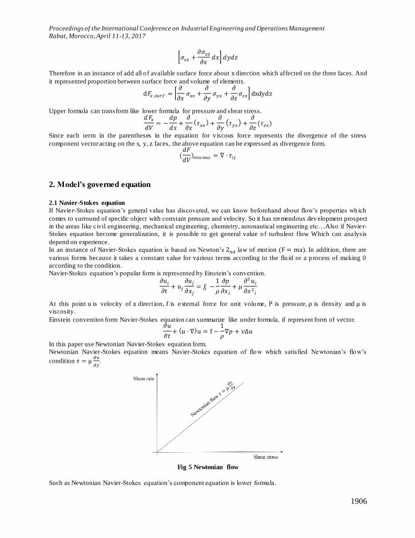
In the case of surface fo rces, it is the force due to the stress acting on the surface. At this t ime, the sum of the shear

stress 𝜏𝑖𝑗 related to the hydrostatic pressure and the velocity gradient is the sum of the total surface forces of the

surface forces. Unlike the velocity with three components, the shear stress 𝜏𝑖𝑗 , the stress 𝜎𝑖𝑗, and the strain 𝜖𝑖𝑗 are all

nine tensors, and each component has two subscripts, unlike the one with a subscript. The suffix ind icates the

direction of the surface to which it belongs, and the suffix j indicates the direction in which the force acts.

Fig 4 stress on 𝐱, 𝐲, 𝐳 faces

For example In an instance of momentum, If input value is 𝜎𝑧𝑧 𝑑𝑦𝑑𝑧, out value is become control’s volumes inner

change value like lower formula.



1906

[𝜎𝑧𝑧 +𝜕𝜎𝑧𝑧

𝜕𝑥𝑑𝑥] 𝑑𝑦𝑑𝑧

Therefore in an instance of add all o f available surface force about x direction which affected on the three faces. And

it represented proportion between surface force and volume of elements.

d𝐹𝑥 ,𝑠𝑢𝑟𝑓 = [𝜕

𝜕𝑥𝜎𝑥𝑥 +

𝜕

𝜕𝑦𝜎𝑦𝑥 +

𝜕

𝜕𝑧𝜎𝑧𝑥] dxdydz

Upper formula can transform like lower formula for pressure and shear stress. 𝑑 𝐹𝑥

𝑑𝑉= −

𝑑𝑝

𝑑𝑥+

𝜕

𝜕𝑥(𝜏𝑥𝑥

) +𝜕

𝜕𝑦(𝜏𝑦𝑥) +

𝜕

𝜕𝑧(𝜏𝑧𝑥)

Since each term in the parentheses in the equation for v iscous force represents the divergence of the stress

component vector acting on the x, y, z faces, the above equation can be expressed as divergence form.

(𝑑𝐹

𝑑𝑉)𝑣𝑖𝑠𝑐𝑜𝑢𝑠 = ∇ ∙ 𝜏𝑖𝑗

2. Model’s governed equation

2.1 Navier-Stokes equation

If Navier-Stokes equation’s general value has discovered, we can know beforehand about flow’s properties which

comes to surround of specific object with constant pressure and velocity. So it has tremendous dev elopment prospect

in the areas like civil engineering, mechanical engineering, chemistry, aeronautical engineering etc…Also if Navier-

Stokes equation become generalization, it is possible to get general value o f turbulent flow Which can analysis

depend on experience.

In an instance of Navier-Stokes equation is based on Newton’s 2𝑛𝑑 law of mot ion (F = ma). In addit ion, there are

various forms because it takes a constant value for various terms according to the flu id or a p rocess of making 0

according to the condition.

Navier-Stokes equation’s popular form is represented by Einstein’s convention.

𝜕𝑢𝑖

𝜕𝑡+ 𝑢𝑗

𝜕𝑢𝑗

𝜕𝑥𝑗

= 𝑓𝑖 −1

𝜌

𝜕𝑝

𝜕𝑥 𝑖

+ 𝜇𝜕2 𝑢𝑖

𝜕𝑥2𝑖

At this point u is velocity of x direct ion, f is external force for unit volume, P is pressure, ρ is density and μ is

viscosity.

Einstein convention form Navier-Stokes equation can summarize like under formula, if represent form of vector. 𝜗𝑢

𝜗𝑡+ (u ∙ ∇)u = f −

1

𝜌∇𝑝 + 𝑣∆𝑢

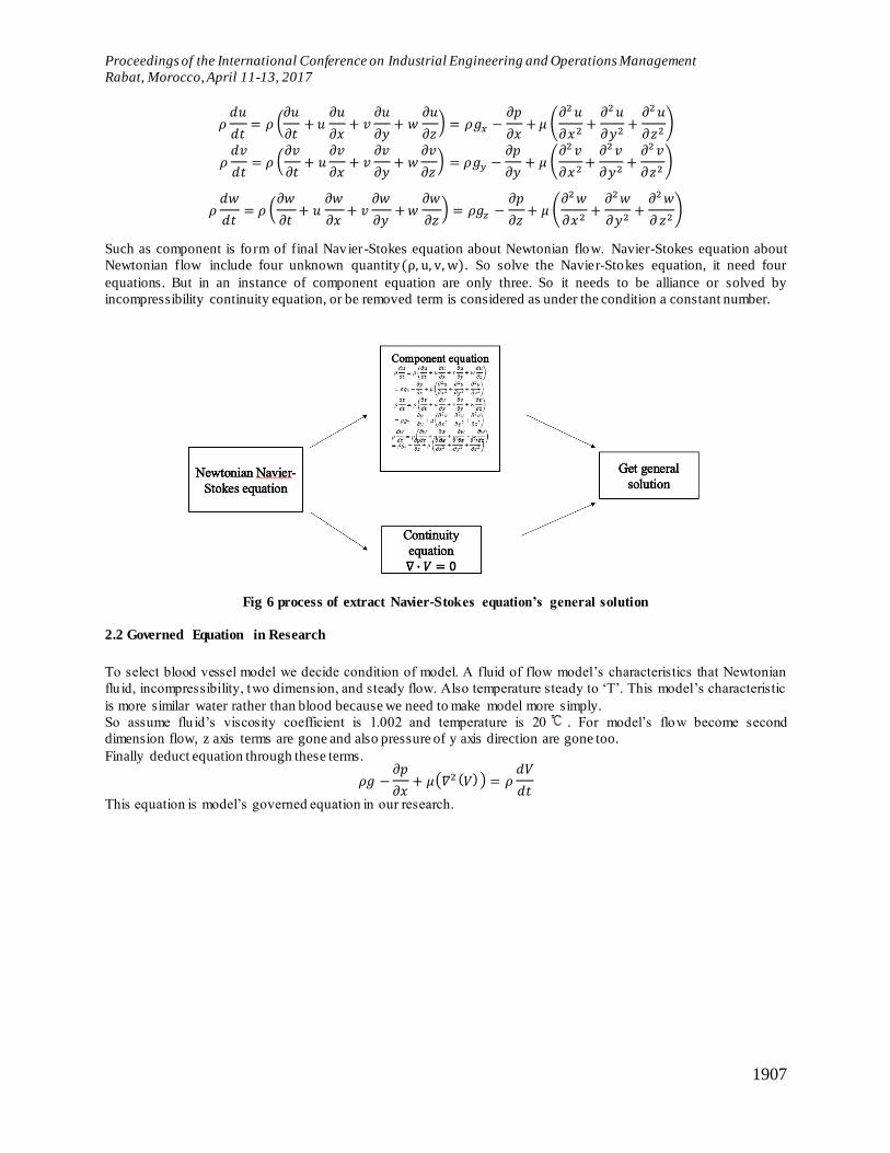
In this paper use Newtonian Navier-Stokes equation form.

Newtonian Navier-Stokes equation means Navier-Stokes equation of flow which satisfied Newtonian’s flow’s

condition τ = μ𝑑𝑢

𝑑𝑦.

Fig 5 Newtonian flow

Such as Newtonian Navier-Stokes equation’s component equation is lower formula.



1907

𝜌𝑑𝑢

𝑑𝑡= 𝜌 (

𝜕𝑢

𝜕𝑡+ 𝑢

𝜕𝑢

𝜕𝑥+ 𝑣

𝜕𝑢

𝜕𝑦+ 𝑤

𝜕𝑢

𝜕𝑧) = 𝜌𝑔𝑥 −

𝜕𝑝

𝜕𝑥+ 𝜇 (

𝜕2 𝑢

𝜕𝑥2+

𝜕2 𝑢

𝜕𝑦2+

𝜕2 𝑢

𝜕𝑧2)

𝜌𝑑𝑣

𝑑𝑡= 𝜌 (

𝜕𝑣

𝜕𝑡+ 𝑢

𝜕𝑣

𝜕𝑥+ 𝑣

𝜕𝑣

𝜕𝑦+ 𝑤

𝜕𝑣

𝜕𝑧) = 𝜌𝑔𝑦 −

𝜕𝑝

𝜕𝑦+ 𝜇 (

𝜕2 𝑣

𝜕𝑥2+

𝜕2 𝑣

𝜕𝑦2+

𝜕2 𝑣

𝜕𝑧2)

𝜌𝑑𝑤

𝑑𝑡= 𝜌 (

𝜕𝑤

𝜕𝑡+ 𝑢

𝜕𝑤

𝜕𝑥+ 𝑣

𝜕𝑤

𝜕𝑦+ 𝑤

𝜕𝑤

𝜕𝑧) = 𝜌𝑔𝑧 −

𝜕𝑝

𝜕𝑧+ 𝜇 (

𝜕2 𝑤

𝜕𝑥2+

𝜕2 𝑤

𝜕𝑦2+

𝜕2 𝑤

𝜕 𝑧2)

Such as component is fo rm of final Navier-Stokes equation about Newtonian flow. Navier-Stokes equation about

Newtonian flow include four unknown quantity(ρ, u, v, w). So solve the Navier-Stokes equation, it need four

equations. But in an instance of component equation are only three. So it needs to be alliance or solved by

incompressibility continuity equation, or be removed term is considered as under the condition a constant number.

Fig 6 process of extract Navier-Stokes equation’s general solution

2.2 Governed Equation in Research

To select blood vessel model we decide condition of model. A fluid of flow model’s characteristics that Newtonian

flu id, incompressibility, two dimension, and steady flow. Also temperature steady to ‘T’. This model’s characteristic

is more similar water rather than blood because we need to make model more simply.

So assume flu id’s viscosity coefficient is 1.002 and temperature is 20 . For model’s flow become second

dimension flow, z axis terms are gone and also pressure of y axis direction are gone too.

Finally deduct equation through these terms.

𝜌𝑔 −𝜕𝑝

𝜕𝑥+ 𝜇(𝛻2 (𝑉) ) = 𝜌

𝑑𝑉

𝑑𝑡

This equation is model’s governed equation in our research.



1908

Fig 7 process of establish governed equation.

3. Interpretation about CFD (Computational Fluid Dynamics)

3.1 Produce and Verify the Code

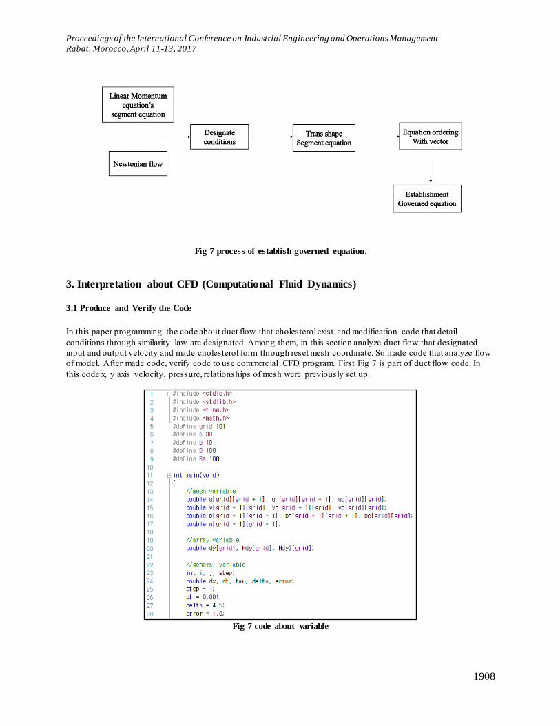
In this paper programming the code about duct flow that cholesterol exist and modification code that detail

conditions through similarity law are designated. Among them, in this section analyze duct flow that designated

input and output velocity and made cholesterol form through reset mesh coordinate. So made code that analyze flow

of model. After made code, verify code to use commercial CFD program. First Fig 7 is part of duct flow code. In

this code x, y axis velocity, pressure, relationships of mesh were previously set up.

Fig 7 code about variable



1909

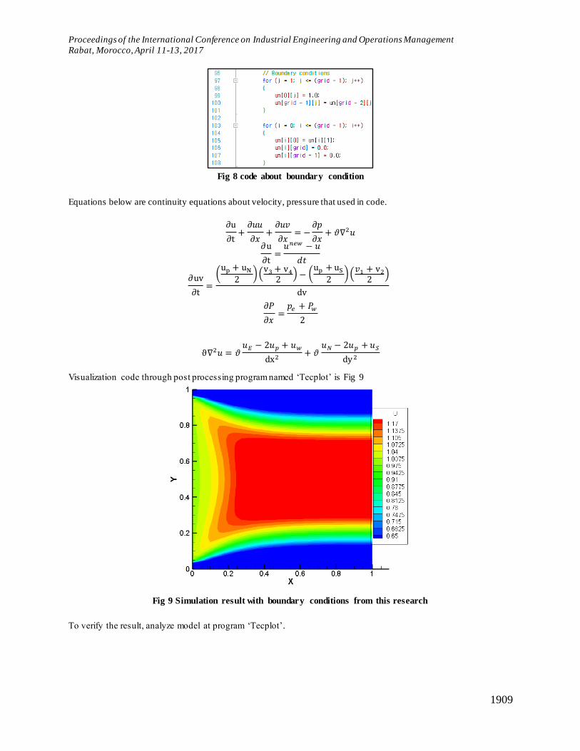
Fig 8 code about boundary condition

Equations below are continuity equations about velocity, pressure that used in code.

∂u

∂t+

𝜕𝑢𝑢

𝜕𝑥+

𝜕𝑢𝑣

𝜕𝑥= −

𝜕𝑝

𝜕𝑥+ 𝜗∇2𝑢

∂u

∂t=

𝑢𝑛𝑒𝑤 − 𝑢

𝑑𝑡

∂uv

∂t=

(up + uN

2) (

v3 + v4

2) − (

up + uS

2) (

𝑣1 + v2

2)

dv

𝜕𝑃

𝜕𝑥=

𝑝𝑒 + 𝑃𝑤

2

ϑ∇2𝑢 = 𝜗𝑢𝐸 − 2𝑢𝑝 + 𝑢𝑤

dx2+ 𝜗

𝑢𝑁 − 2𝑢𝑝 + 𝑢𝑆

dy 2

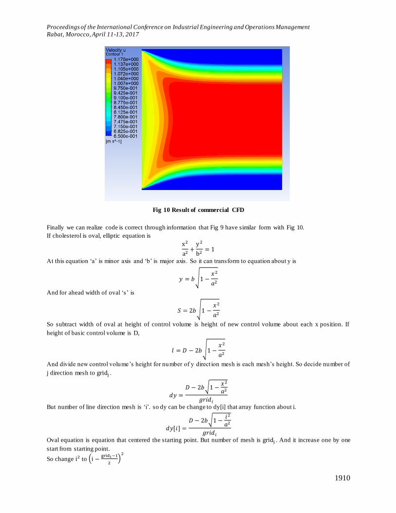
Visualization code through post processing program named ‘Tecplot’ is Fig 9

Fig 9 Simulation result with boundary conditions from this research

To verify the result, analyze model at program ‘Tecplot’.



1910

Fig 10 Result of commercial CFD

Finally we can realize code is correct through information that Fig 9 have similar form with Fig 10.

If cholesterol is oval, elliptic equation is

x2

a2+

y 2

b2= 1

At this equation ‘a’ is minor axis and ‘b’ is major axis. So it can transform to equation about y is

𝑦 = 𝑏√1 −𝑥2

𝑎2

And for ahead width of oval ‘s’ is

𝑆 = 2𝑏√1 −𝑥2

𝑎2

So subtract width of oval at height of control volume is height of new control volume about each x position. If

height of basic control volume is D,

𝑙 = 𝐷 − 2𝑏√1 −𝑥2

𝑎2

And divide new control volume’s height for number of y direct ion mesh is each mesh’s height. So decide number of

j direction mesh to gridj .

𝑑𝑦 =𝐷 − 2𝑏√1 −

𝑥2

𝑎2

𝑔𝑟𝑖𝑑𝑖

But number of line direction mesh is ‘i’. so dy can be change to dy[i] that array function about i.

𝑑𝑦[𝑖] =𝐷 − 2𝑏√1 −

𝑖2

𝑎2


Oval equation is equation that centered the starting point. But number of mesh is gridj . And it increase one by one

start from starting point.

So change i2 to (i −gridi −1

2)

2



1911

𝑑𝑦[𝑖] =𝐷 − 2𝑏

√1 −

(𝑖 −𝑔𝑖𝑟𝑑𝑖 − 1

2)

2

𝑎2


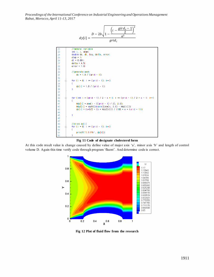
Fig 11 Code of designate cholesterol form

At this code result value is change caused by define value of major axis ‘a’, minor axis ‘b’ and length of control

volume D. Again this time verify code through program ‘fluent’. And determine code is correct.

Fig 12 Plot of fluid flow from the research



1912

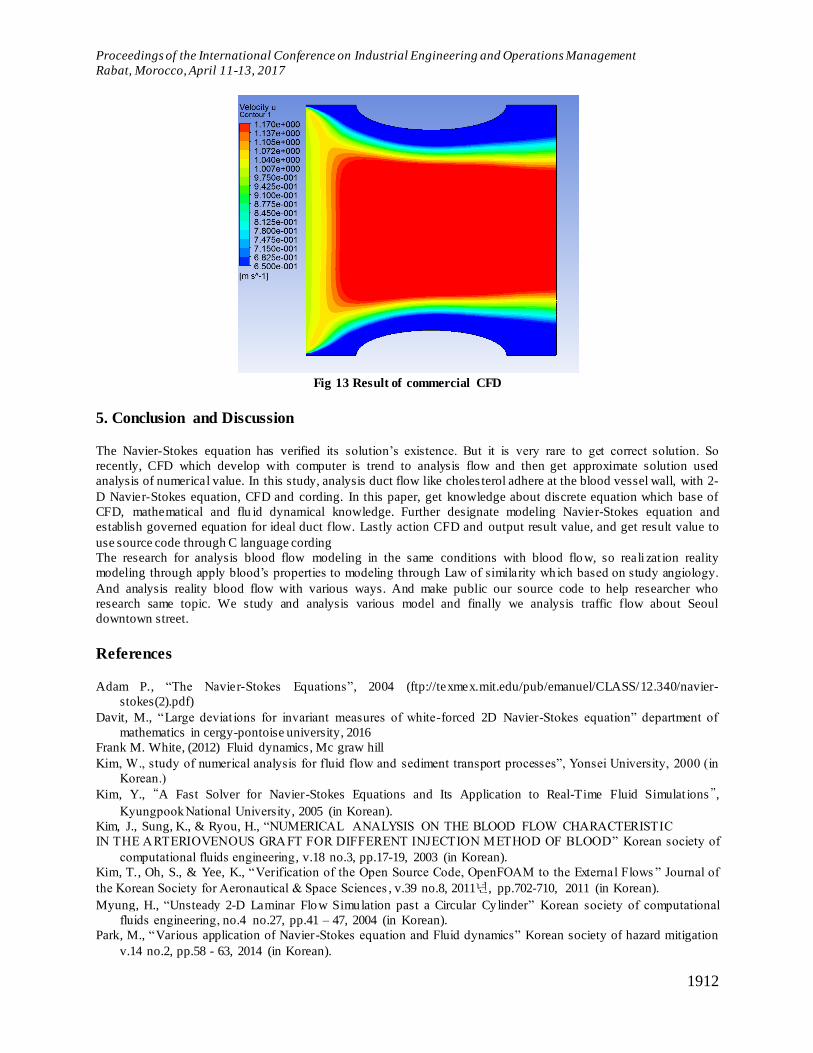
Fig 13 Result of commercial CFD

5. Conclusion and Discussion

The Navier-Stokes equation has verified its solution’s existence. But it is very rare to get correct solution. So

recently, CFD which develop with computer is trend to analysis flow and then get approximate solution used

analysis of numerical value. In this study, analysis duct flow like choles terol adhere at the blood vessel wall, with 2-

D Navier-Stokes equation, CFD and cording. In this paper, get knowledge about discrete equation which base of

CFD, mathematical and flu id dynamical knowledge. Further designate modeling Navier-Stokes equation and

establish governed equation for ideal duct flow. Lastly action CFD and output result value, and get result value to

use source code through C language cording

The research for analysis blood flow modeling in the same conditions with blood flow, so reali zat ion reality

modeling through apply blood’s properties to modeling through Law of similarity which based on study angiology.

And analysis reality blood flow with various ways. And make public our source code to help researcher who

research same topic. We study and analysis various model and finally we analysis traffic flow about Seoul

downtown street.

References

Adam P., “The Navier-Stokes Equations”, 2004 (ftp://texmex.mit.edu/pub/emanuel/CLASS/12.340/navier-

stokes(2).pdf)

Davit, M., “Large deviat ions for invariant measures of white-forced 2D Navier-Stokes equation” department of

mathematics in cergy-pontoise university, 2016

Frank M. White, (2012) Fluid dynamics, Mc graw hill

Kim, W., study of numerical analysis for fluid flow and sediment transport processes”, Yonsei University, 2000 (in

Korean.)

Kim, Y., “A Fast Solver for Navier-Stokes Equations and Its Application to Real-Time Fluid Simulat ions”,

Kyungpook National University , 2005 (in Korean).

Kim, J., Sung, K., & Ryou, H., “NUMERICAL ANALYSIS ON THE BLOOD FLOW CHARACTERISTIC

IN THE ARTERIOVENOUS GRAFT FOR DIFFERENT INJECTION METHOD OF BLOOD” Korean society of

computational fluids engineering , v.18 no.3, pp.17-19, 2003 (in Korean).

Kim, T., Oh, S., & Yee, K., “Verification of the Open Source Code, OpenFOAM to the External Flows ” Journal of

the Korean Society for Aeronautical & Space Sciences , v.39 no.8, 2011년, pp.702-710, 2011 (in Korean).

Myung, H., “Unsteady 2-D Laminar Flow Simulation past a Circular Cylinder” Korean society of computational

fluids engineering, no.4 no.27, pp.41 – 47, 2004 (in Korean).

Park, M., “Various application of Navier-Stokes equation and Fluid dynamics” Korean society of hazard mitigation

v.14 no.2, pp.58 - 63, 2014 (in Korean).



1913

Myung, H., (2012), CFD, Myun Un Dang, Seoul

Jang, T., “Flow Induced Vibration Analysis Using Two-Dimensional Incompressible Navier-Stokes Equations”,

Korea Institute of Science and Technology, 2002 (in Korean).

Jang, S., “A Numerical Study on The Characteristics of The Fluid Flow in A Backward-Facing Step Channel with A

Porous Body” ,Korea Institute of Science and Technology, 1986 (in Korean).

Suh, S., & Yoo, S., “Steady Flow Analyses of Blood Analogue Fluids in the Stenosed Circu lar and Bifurcated

Tubes”, Korea-Australia Rheology Journal, v.7, no.2, pp. 150-157, 1995 (in Korean). Kim, Hyea-Hyun. “Numerical analysis of Navier-Stokes equations”, Korea Institute of Science and Technology,

1999 (in Korean)

http://www.riss.kr/search/detail/DetailView.do?p_mat_type=be54d9b8bc7cdb09&control_no=17f8dd1784261d4fffe0bdc3ef48d419

Documents

Modeling and Simulating Flow Phenomenon using Navier