Embed Size (px)
Citation preview

A K Peters, Ltd.
ISBN 1-56881-159-4
ì<(sl&q)=ibbfji< +^-Ä-U-Ä-U
Computer Algebra andSymbolic ComputationM a t h e m a t i c a l M e t h o d s
J O E L S . C O H E NComputer Algebra andSymbolic ComputationM a t h e m a t i c a l M e t h o d s
J O E L S . C O H E N
Mathematica™, Maple™, and similar software packages provideprograms that carry out sophisticated mathematical operations. Inthis book the author explores the mathematical methods that formthe basis for such programs, in particular the application of algorithmsto methods such as automatic simplification, polynomial decomposition,and polynomial factorization. Computer Algebra and SymbolicComputation: Mathematical Methods goes beyond the basics ofcomputer algebra—presented in Computer Algebra and SymbolicComputation: Elementary Algorithms—to explore complexity analysisof algorithms and recent developments in the field.
This text:
• is well-suited for self-study and can be used as the basis for a graduate course.
• maintains the style set by Elementary Algorithms and explains mathematical methods as needed.
• introduces advanced methods to treat complex operations.• presents implementations in such programs as Mathematica™
and Maple™.• includes a CD with the complete text, hyperlinks, and algorithms
as well as additional reference files.
For the student, Mathematical Methods is an essential companion toElementary Algorithms, illustrating applications of basic ideas. Forthe professional, Mathematical Methods is a look at new applicationsof familiar concepts.
A KPETERS
Computer Algebra and Symbolic Computation
Cohen
Math
em
atical Me
tho
ds


����������� �������� ���������������

����������� �������� ����������������������������������
���������������������� ��� ����������
����������� ������
������������� �������������

������������������ �������������������������������� ���������������
�������������� ������������������������������������������������������������� �����!"� ���#�#����������$��������#��������!%���������������������������#�������&�#����!� � ��������#����'����#�!��������(������&�)*��+� ���+���+���������,��� �-.�����#�!!�����&��/�����
0,������1��� ����������-�#��������������������������������������������������������������������������
1������������!������!���������2�#��3''�#�,�4������!��5��� ��������,2����*��#6��7,����� �888�6�����!�#��
��"�������9������� "�,�4������!��5���
,��������!���!��2����*�������'�����������������#���� "����!�#��"����������#��"� ���������#�����������:�������"�'��������#�����#������#���#�����#�����������#��"�������#����������� "��"���'��������!���������������2��!"!����8�������8������������!!����'��������#��"�������8����

������������ ����

vii
Contents
1 Preface ix
1 Background Concepts 11.1 Computer Algebra Systems . . . . . . . . . . . . . . . . . . . . 11.2 Mathematical Pseudo-Language (MPL) . . . . . . . . . . . . . 21.3 Automatic Simplification and Expression Structure . . . . . . 51.4 General Polynomial Expressions . . . . . . . . . . . . . . . . . 111.5 Miscellaneous Operators . . . . . . . . . . . . . . . . . . . . . 12
2 Integers, Rational Numbers, and Fields 172.1 The Integers . . . . . . . . . . . . . . . . . . . . . . . . . . . . 172.2 Rational Number Arithmetic . . . . . . . . . . . . . . . . . . . 372.3 Fields . . . . . . . . . . . . . . . . . . . . . . . . . . . . . . . . 44
3 Automatic Simplification 633.1 The Goal of Automatic Simplification . . . . . . . . . . . . . . 633.2 An Automatic Simplification Algorithm . . . . . . . . . . . . . 91
4 Single Variable Polynomials 1114.1 Elementary Concepts and Polynomial Division . . . . . . . . . 1114.2 Greatest Common Divisors in F[x] . . . . . . . . . . . . . . . . 1264.3 Computations in Elementary Algebraic Number Fields . . . . 1464.4 Partial Fraction Expansion in F(x) . . . . . . . . . . . . . . . . 166

viii
5 Polynomial Decomposition 1795.1 Theoretical Background . . . . . . . . . . . . . . . . . . . . 1805.2 A Decomposition Algorithm . . . . . . . . . . . . . . . . . 188
6 Multivariate Polynomials 2016.1 Multivariate Polynomials and Integral Domains . . . . . . . 2016.2 Polynomial Division and Expansion . . . . . . . . . . . . . . 2076.3 Greatest Common Divisors . . . . . . . . . . . . . . . . . . 229
7 The Resultant 2657.1 The Resultant Concept . . . . . . . . . . . . . . . . . . . . 2657.2 Polynomial Relations for Explicit Algebraic Numbers . . . . 289
8 Polynomial Simplification with Side Relations 2978.1 Multiple Division and Reduction . . . . . . . . . . . . . . . 2978.2 Equivalence, Simplification, and Ideals . . . . . . . . . . . 3188.3 A Simplification Algorithm . . . . . . . . . . . . . . . . . . 334
9 Polynomial Factorization 3499.1 Square-Free Polynomials and Factorization . . . . . . . . . 3509.2 Irreducible Factorization: The Classical Approach . . . . . 3609.3 Factorization in Zp[x] . . . . . . . . . . . . . . . . . . . . . 3709.4 Irreducible Factorization: A Modern Approach . . . . . . . 399
Bibliography 431
Index 441
�����
������ �� �� �� �� �� �- ���������� ��� ������ ����� ���� �������� <��� �� �1������9 ������������9 ��� ����������� �- �� ������� ���� ��������� ��� �����: ����������� "�������� '��� ���5��� �� ��������� �"�9 �������� ���� �� ������� ������ ����������� �� ��������9 � �� ����������� �� �� ���=�� ���� ���������� ��� �������� ��� �������� ������� ������ �� �������� �������� �������� ���> �� �� ������ <��� �� -��������� �- �� ������ �������1 �������� ����������� ������ ��� <��� �� ������������ �-��� �� ������ �� ��� �- �� �������� ��� ������ ������� �1�������� ������ �� �� �� ����� ��� �� �� '��� ���59 <���� �������� �������� �����9 �� ������ <��� �� ����� ����������� ��� �� �������� ������� ���� � �� -��������� �- �� ���=��� 4��� ���5� �1�� � ��� ��<� �"�� ��� ������� ���� ���< ��< �� �� �������� �� ��-�<� ��� ����� �1� �"�� ���� ����� �� ������ �� ��-�-��� �- �� ���
'�� ���5� ��1 �� �� 1����� ��� � �- �1������ -� �1 �#���� '�� � ���� �� �� ����� ���� -� � �<��8��� ���� �8����� ������ �� �� ���� ��� �� �?� �� �� @��1���� �- 0�1 1���� �� -� �� ���� �. ���� '� �� ����9 <���� �� �� ����� -� ������� �� ��������9 ������� ������� ��� ����� ������� ��� � -< ����� ������� -�� ����������9 ������ �����9 ��� � ���� �'� ����� ����9 <���� �� �� ����� -� � ���� ��� �������9 �������������� ����� ������� �� ���� ���������� ��� ������ ������'� ���� �� ���������� ��� ���� ���������� ��� ������ ������
�
��� ��
�����1�������
'� �� � ������ -� ��� ���5� ������� ������� ��� ��-��������-�� ����������9 ������ �����9 ��� ��� �������� ��� <�� <������5 �� 5��< ����� ������ �� �� ��� ��� �������������
(� �� ����� �- �� ���������� �"�9 < ��1 ��� �� ������: ���8������� '� ����������� �8������ ������ �� ����� �<� ��-�����A������� �8��� �- ����� ��������� ���� � �����1�������������9 ������ ���� �� ��9 ��� ������ ������ ��?����� 8���������� (� ��������9 �� ���������� ���� �� ����� ���������� �� �������� ����� ����������� ��������� �� ��� �� � ���- �����8����� ����� '����� -�� ������ ���� ���� ��� ������� �� ��� �������� �� ����
&� �� ������ ����� ���9 < ����� ���� �� �� ��� ��� ���"���� <��� � ������ �� ����� ��� �� ���� �� ,����9 ������9�9 �BB9 � C�1�� ������ � ��� ��� �� � � ��� ��� �� ��� ���5�9�� �5���� �� ����� ���1�� ��� �� ����� �1������ ������� �� � �� ����� �� ����� ���� � �������� &� �� ����� �����8����� �� �������� �������� �� ������ �� �� �� ������� ������ ����� ������� <��� ��1 �� ������ �� � ���1������� �� ����� ����9 �� ����� �� ������ �� ����� # �- ������ �� �������� -��� ������ �� �� ������1�
*����������� ���5�� 9 <��� ��� �8������ ��D� �� � -���� ���-� ���� ���5�9 �� � �������� ��� �� � ��� ������� �� �� �"���� �� <� �� ����������� ��� ������������� �������������� ��8���� ������ � �� ����������� �1������ �� ��� ������� ��� ������� �� -� ������� <��� �� ������� �8������9 �� �� ������� ��������9 ��� ��� ������� ��1�� � ��������� �� �� ��1����������� �- �� ���=���
2����0���� �� �������4����� ���5�� 9 ��� ���5� � ������ �� �1 �<� ������������������;
� �� ������� ������ ��� ���� �� �� ��� ��������� ����� ���� ���������� ���� �� � ���� ��� ���� ����� �� �������� ���� ����� ����� ��� ���
�� ������� ������ �� ���������� ���������� � ������� ��� ������ <��� �� ������� -���� �� ������� ���������� � ���1������������� �� ����� � ,� "����9 �� �� ����� -� �� "������� �-������� ��� ��<� �- ����������� �� ������� �1� ��-������ ������ �-<��� �����1� ������ ���� ��� � "���� �� � ������ �� ���

��� �� �
'� ������ �� ������ �� �������� �� ������ <��� �� �� �������� -��������� �- ��������� �� ������ �������� ����������� �������� '� 1�<����� �� ���� ����������� "�������9 ����� �� "������� ��9 � �� ���� ��=��� �- ������ �� �� �� ���9 ���9���� � -< ������1 �������� ���� �����: ��� �������� "�������9< ��� ������� ���� ������ �������� -�� �� ��9 �� ������9��������9 ��� ��?����� 8�������� ,� "����9 �� ������ � �1� -��� �������� ��� ������������ �- ����������� ��� ������� "�������9 �������������� �- "�������� ��� �� ������� -��������9 ��?��������9������ ��� �����9 ��� �� �������� �- �� �� ��?����� 8��������� ���� �- �� ������ �� ���� ���5 �� ��� -���� �� ��� �����������"����5� � �� ���9 �� ��1���� ������ �� �� �"����5��
� �� �������� ���� �� ��� � ���� ��� �������� �� ��������� ����������� ������� �� ������ �������� ���� ���� ���
,� �� ���� �# ���9 �� ���� �� ������ �� �� ��� �� ������� <��� �� �1������ �- ?���1 ��� D���� �� ������ -� ��������������� �������� �������� ���������� ���� ������ ��1���� ��� �����������9 ���������� -�����:�����9 ���������� ������������9�� �������� �- ������ �- ���� 8������� ��� �����1���� ����������8�������9 ��� ��� ��� �����9 ��� �� �������� �- ��?����� 8�������������� � �� ������ -� ��� �- ��� ������ ��1 �� 5��<� ���� ��������� �����9 -� D����� ����� ��� � ��� ������� �� �������� �� ������ -� ������ �� �� ��-�<�� '� ��������� �� ������� ��������9 ��<19 ����� ��� � ���� ����� ��� ��1�� � �����"� �� ����1�� �� ����� �� ���� ���� ��� �� �� -� �� D�������������
'� ������ �� � ���� ��� ������� �� �� ����������� �� �� ������������ �����8�� ��� �� ������� ������ �- ������ �� ��� ������� � �� ������ �� ���� ���5 �� �� ��D���� ��� 8��� �� ������������ ��������������9 �� ������� ��� ������� �- ������ �� ��� �� ������ �� �� �������� ��� ������� �� �� ������ ������� �� ������� �1� -� ����� ��� ��� ������� ���� ��������9 ��������� ���-����� ������ ������ �- �� ���� "�������9 ���� ������ ��1�������������� -� ��� � ��� �����1���� �����������9 ������� �����������9���������� ������������9 ���������� ������ ������ <��� %E��� ����9��� ���������� -�����:������
,���� !��������'� ����� �- �� ���������� �"� ����� � ������ ���� �� �� �� -���<��� � ��D���� ������� ����� <���� ������ ��� �� ������ �� ������ �� �

�� ��� ��
�"�� '��� ������� �� ��������� �� �� ���5 ���� �- �� ������9 ������������� ��D����� �- �� ������ ���9 �- ����9 �� ���� ������������(� ��������9 < ���1 ���� �� ���������� �"� ������ ���� � �� ������������ �� �� ���=�� ���� ������ ��� �- �� �������� ����� �� �� �� ��� ������ ��� �� �� � ��������1 � ������ ��� ����� �-� �������� ����� � �� ������ '��� 1�<����� ��� ���� �� ������� �-������9 ����� �- �� ������9 ��� �1� �- ����������� � ��
,� "����9 ���������� �� ����������� �� �� �������� ����� ��� ���� ��� ������� ���� ����� �� ������� �� �� ���� �������� �� ��-�<�� F ����� ��������� !������� �� ������ -� ���� ���� � ��� �����1���� ����������� <��� ������� ���� ��D����� ��� �!������� �� ����� -� ��� � 1����� ����������� <��� ����� �� �������� ��D������ (� �� <�� 5��<�9 ��<19 ����9 -� D����� ������9 ��� �� ������ � ��� ������� �� ��� ����� �� ������ ��� ������ �� �� ������ ,� ���� ����9 < ����� �� �� ���1���� ���������� �� �� ����� -� �����1���� ����������� ��� ������ ����������� =���� ������9 <���� �� 8��� ��1��1� ��� -� ������ ������ ��� ����� �- ��� ���5��
&� ����� ���� �� ��� �������� �� �� ���������� �����"��� �- ����� ��� ���� 8������ �- �� ������� �����"��� �������� -� ������� �� ��9 <���� �� �-�� 8��� ��1��1�9 ��� �����8�� -�� �� �������������9 ���������� ����9 ����� ����������9 �� ���� �- ������������9 ��� ��� ��� ���� � <�� ����� �� ���5 ���� �- �� ������������� &- ����9 �� �� ��������� �� � �� D����� ������������ ������ ���9 <�� ��������9 < ������� �������� �� "����� ��� �- ������� ���� ���� � ���� ���� �� � ���� ��� ������� �� �� ���� ��8����� -� � ����� �1� ���� ���� ������� �� �����"��� ���������- �� ������ ���� <��� ��� �1������� �� �� ����
�-���� !�������� �� ������ ��������� �- �� ������ ��1� �� ��� ���5� �� �1��� �� -����<�� ����� ��������
3�������% ������-��������� � ���� ������ �� �������� �������� '��� �����
�� �� ����������� �� �� �� �- ������ �� ��� (� ��������� ���� �������������� ��� ����������� -� ������ �������� ����������� ���� ������ �� <��� � ���� �- �������� ������ �� �� �������
�� �������� ���� ����� ���� � ���� �� ��� �� ��� ����� ������� ���� �������������� ��� �� ��� ����� �������� � �� �������� ��� !"���#����� � $�� ������ � %�� ����� ������ ��� ������� �� �� &������ �'('�� )�� �'(*�� �� +����� �'(%�,

��� �� ���
������� � ���������� �������� �� �������� �������� '�������� �������� �� �� ������� ��� �� ����� � ���� ��� ������� ��� �� �� ������ ���� ���� �� ��� ���� ���� �� ���5� �� ����� ���������9 "�����9 ��� �� ������ �- ������ �� ��� ��� �� � �������� �� ���� ��� � ����� �������� ���� �� ������� ��� ���������1������ �� ���� ������ �� �� ��� �� �� '��� ����� ���� �������� ��� ��������� �- �� 1�������� ����� �� ������ �� �� ��-�<���������� ��������� ������ ������� ��� � ��� ����� <���� ������� ����� �� �� ���� ������� �� ���� �- -�� �- 8������� "���������� ������� �- ����������
������� � ��������� ��������� �� ����������� �!����������'��� ����� �� ������ <��� �� ������ � ������ �- ������������ "�������� 4��� �� ���1������� ������ ��-� 1��������� ����� ������ � ������ ��-� 1�������� ��� ��������� ������ ������� �������� '� ������ �- ������������� ������ � "������� �� ��������� ����� ��� �� ������ ����� ���� �� ����� ���� �� �� ���� -���,�� ������1 ��� ������ �����9 �����9 ���� �� ������9��� ���������� ���� �����: ��� �������� ����������� "������� ���������� '� ����� ���� ������� � ��������� �- -�� ��� ������� �!��� �� 9 ����������9 �������� ����������9 ��� ���������� �����������<���� ���� ���� �� �� � ������ �- �� "�������
������� " ���������� ����������� ����������� (� ���� ������ < ����� �� ����� �� ����� ������� �� ��� ��� �� ���������� �� ����� � ���� �- ������ �� ������� '� ������������ � ��� ����� <���� ������ �� �� ����� ���� ���1� � ����� �- �� �� ������ ��?����� 8������� ���� �� �������� �- 1�����������8� ��� �� ����� �- "��� 8������� <��� ��� ���� -������
������� # ��������� ����������� '��� ����� ������ ������� �� � �� ����� �����8� �� ������ �� �� ��� �1� � �����- "����� ���� �������� ��� ��1���� � ��� ������������ (� ������� � �������� ���� ������ �� ������ ��� ����� �� ����� <���� ��� ��������1���1� -� � ������ ����� �- -�������� ���� �� ���� ������ �-�� ��� �� ��� �� ������������ ������ !"������� �- �� �� ����� �������� �� ������ ������� -������� ��� �����9 ��� �� ���������� ���9 ������ ��� ����� �� ����9 ��� �� �� ���� -������� -��� ������ �� �� "�����
������� $ ��������� �� %���������� �� �������� �!����&������ '��� ����� �� ������ <��� �� �� ������ ���� �����: ��� ���������� ����������� ��� ������� "�������� (� ������� �������������� ������� -� 1����� ������ �- ����������� ��� ������� "������� ����� ���� �� �� ������ � ������ �- "�������� �� ������ ������ �� ������1 �������� �������� �� ����� � � �1� -� �

�� ��� ��
��� ��D���� �����������9 ��D���� ���������9 "�������9 ��� ���������:����� �- �� ���� "��������������� ' �!��������� �� (������������ (���������������
'��� ����� �� ������ <��� �� ������ ���� ��������� "�������� ����� ������� -��������� (� ������� �� ������ -� "�������� "���������� �������9 �� ������� "������� ��� �������9 ��� � ������ �������� ����� ���� ��� 1�-� � �� ����� �- �� ������� ���������
)�-������ )��-���������� � )��*����� ��������� '��� ����� �� � ������ �- ��
���5 ���� ������ -�� ������ �� �������� ���� ��1��� � -���<�5 -� �� ����������� ��� ������������� ����������� �� �� ���5� (�������� � ��������� �- �� ����������� ��������� �� �����9 � ��-���������� �- �� � ������ ��� ���������� ������ �- �� ���� "��������9 ��� � ������ �- �� ����� ����������� ������ ���� ������ �� �� �������������� � �������+ �������� ,������+ �� -��� �� '��� �����
� �� ������ <��� �� ������� ��=��� ���� ��� �� ������ �� ��9�������� ��� �9 ������� �����9 ��� �� ���� ������ (� �������!�����G� �� ����� -� �� ���� ������ ��1��� �- �<� ��� �9 ��"���� !������� �� �����9 �� ����� ����� �� �����9 ��� ������� ������ �� ����� ���� ����-��� �� ��1��1� �������� "������<��� ��� � ��� -������� �� � ������� ���� �� ������� -��� (� ���������9 �� �������� �� ������ �- � �� <���� ������ �� � ��� <���� ������ �- ���� ������ ���� ��� �� ������ �� ���������� � ��������� ������.������� ��������� ������ ������
�� � �� �� �� ��������� �- �� ���� ��� �� ������� ������ ����������-�������� ���� � ������ �� �� "������ �� ��� �- �� 1�������������� (� ���� ����� < ��5 �� ������� ���5 �� �� �� ���� ��������� �- ���� �����9 �1 � ���� � ������ �- �� ������������� ������ �"������9 ��� ����� �� ���1��1�� �� ����� ���� ����-��� ������������ "������� �� ������������� ������ � -��� ������ � ��������������� ������ �� ������� -� �� ������� �- ������ �� �� ��-�<�9���� �� �� ���� ������ ������ �- �� ����� �� �� �"����5 �������������� " ������ /������� %����������� '��� ����� �� ����
��� <��� �� ������ -� ��� � 1����� ����������� <��� ��D����� ��� ��� ��� �� ������ �� ���� ����� � ��������� ���� �� ������������1������ (� ������� �� ������ -� ���������� ��1����� ��� "�������9!�����G� �� ����� -� ���� ������ ��1��� �����������9 �� "����!������� �� �����9 ��� � ���������� 1���� �- �� ����� ������� ������ (� ��������9 �� ����� ���������� ��1����� ��� �� �� ������
��� �� �
� ��� �� �1 �� ������ -� ������� ������������ �� ������ ��� ���� ���� ���� '�� �� ������ � ��� ��� �� �1��� ��1�������� �� �� ������ -� ����������� <��� �� ���� ���� ��D������ '������ �������� <��� �� �� ����� -� ������ -������ "������� ���� ������ �� �� "���� !������� �� ������������� # %��������� 0������������� ���������� ���������
���� �� � ����� ���� ������ �- � ���������� ��� � ����� �� ������������ �- ��< � ������������ (� ���� ����� < ������� ����������� ������ �- �� ������������ ����� ��� �1 �� �� ��������� �� ���������� -�����:����� ���� ��� ��� � ������������ � ������� ���� �� ������������ "������������ $ ����������� %����������� '��� ����� ����:�
�� ��1����� ��� �� �� ������ �� �����1���� ����������� <��� ��-� ����� �� �� ��� �� ������� (� ������� �� ������ -� �� ����������� ��1����� �������� �����1 ��1�����9 ������������� ��1�����9 �����������1������9 ���������� "������� ��������� �� ����������� �� ���� ���� ������������ ������9 ��� �� ������1 ��� ���������� �� ������� -� �� ������������������� ' (�� ���������� '��� ����� �������� �� ������� �-
�<� �����������9 <���� �� � �� �� �� �������� �- � ����" <��� ����� ���� �� �� ��D����� �- �� ������������ F ����� � !��������� ����� ��� � ���������� �� ����� -� ������� ����������� ��� ���� ������� �� �� ���������� ������� -� "������ �� ���� ������������� 1 %��������� ������.������ 2��� �� � ����������
'��� ����� ������� �� ����������� �� %E��� ����� ����������� <����� ����������� �� �� ���������� ������ ������ ������ '� ������-� �����������9 < ����� ���� ����������� ��1 ������� ���� ��D�������� �� �� �"��� ������� ���� ���� -� ����������������� 3 %��������� -������4������ '� ��� �- ���� ����� ��
�� ��������� �- � ����� 1���� �- � ���� -�����:����� �� ����� -���� � 1����� ����������� �� 52�3� (� ������� �8���- -�����:����� ��� ������ ��� 52�3 ��� 6�2�3�9 H���5G� ��������� -�����:����� �� �����-� 62�39 4�5���G� �� ����� -� -�����:����� �� 6�2�39 ��� � ����� 1����� �- �� I��� ��-��� �� ������
�������� ����� !��/�� �� �������F �� � ����� ���� �- �� ����� ���� �������� ���� �������� �� �� ����� ������� ��� ���� �- �� ����9 ����������9 �������0 ������ ���9 �� � ��� � 9 �� �� ������� ��� *���������� (� ��������9 ��� �� ������ � ������ �� ����-���������� ���� ������� �� �� ����� ������� ��� �� � �� �� ����������
�� ��� ��
��� ���� ������� @�-��������9 �� �� ����� ���� ��� � ������ ������� ����� �� �� ������� �� �� �"��� ������
'� ����� �� ��� �� ������ �� ��� ���5� ��1 �� ���������� �� ���� )�79 ���������� $��9 ��� ����0 �� �J���� ��7� �������� '� ����� �� ��� �� ��� � -���� �� � �0 ������� <��� �����5�� (� ��� ���59 �1������ ����� �� ��� �� ��� � �������� �� ��<�� K(�����������L -����<� �� � ����� ��� ����9 ����������9� ����0� ����� ����� �� � �� � ������5 -���� ��<� �� ����9 ���� ����������9 ��� ��� �� ����0�9 ��� ������ � �� �"� ����((�-����� �,� "����9 � �� ����� � �� ,� � ��$ �� �� )� ��� ������� �� ,� � ��� �� �� ���� (� ��� "�����9 �� ����� � �������� �- � ������ �� �� ����� �1� �� �� �"� ��� �� ���� � ������ �� �� �� �� ����� �� �
3��������� $������ � �-� ����'�� ���5� ��1 �� ������ �� �� ��'!M�� ����� <��� �� �����������5� 9 <���� ����<� ����"� ���5� �� ����� �����9 ������ �����9�������� ���� ������ -������9 �����9 "�����9 ��9 -�������9"����9 �� ���� �- �������9 �� ���"9 �� ������ ����9 ��� <� ������� ������� 1���� �- �� ���5 ��� <�� �� ���������� -�� ��� ���� ������ ������� -���� ��0,�9 <���� �� �������� <��� �� ���������� ��-�<�9 �� ������� �� �� �0�
����/����������( �� ��-�� �� �� ���� ������� ��� ����� �� <�� �� ��� ������� �������� 1����� �- ���� ���5� '�� ��1��9 ����� ���9�� ������9 ���������9 ��� �������� ��1 ���� ����1� �� ���� ��������� �- �� ���5� '���5� �� +���� 4������9 ���< 4��9 ��"��������9 �� ��� C��5 ����9 *��� �����9 %� 0���1��9 4���0��9 *����� ,�����9 ������� ,�9 ��� %������9 I� %�� 9C����� I������ �9 ��� ���9 N����� ��9 %����� ���9 C��� �� ��9C����� �����9 ������ ����� 9 C��� ���1�9 ������� J��=����9 ���0��� F� ��
( �� ��-�� �� %<� 0��: ��� ��" �������� -� ��� ��� <����� ��'!M ������� ��������> 4���� F�����9 <�� �� ���� �- ���"� ��� �������� ���� �- �� �� ��� �� �� ����0 ��� �� > ������+� ���9 <�� ���� ��� �- �� ��> ��� ������ F�� <�� ��������� ���� �- �� �� ��� �� �� ����������9 ����09 ��� ���������� �� �� '���5� �� ���� 4���9 <�� �� �� ��� ��������� ������ ������ �� ������ ���� ����1� �� "��������9 ��������9 ���

��� �� ���
���� ����-� ���-���� ������� �- �� ���5� I ��-�� ���� �����1�� ������ ���� �������9 ���������9 ��� ����������� ���
( ���� ��5��<�� �� ��� ��� ������ ��� ����� ��� �- ����� �����������9 �� @��1���� �- 0�1� 0��� �� <���� �- �����59 ( <�� �<��� �<� ���������� ��1� �� �1��� ���� �������
������ ����5� �� �� -����� -� ����� ��� ��� ������; �� �������� !��� ��� C����� ����9 0���� ����9 ,���� ����9 ��� �������� !��:���� &���-�
,������9 ( <���� ��5 �� ����5 �� <�-9 H�����9 <�� �� ��� �� �� ������9 ��� ��1� ���� � ��-� �-� ��-� �- ���� ���59 ��� <�� <���������9 ��19 ��� ������ ��� ���� ��5 ���� ���5 ��������
C�� �� ����0�19 �������+�1�� �69 �77�


1
Background Concepts
In this chapter we summarize the background material that provides aframework for the mathematical and computational discussions in the book.A more detailed discussion of this material can be found on the CD thataccompanies this book and in our companion book, Computer Algebra andSymbolic Computation, Elementary Algorithms, (Cohen [24]). Readers whoare familiar with this material may wish to skim this chapter and refer toit as needed.
1.1 Computer Algebra Systems
A computer algebra system (CAS) or symbol manipulation system is a com-puter program that performs symbolic mathematical operations. In thisbook we refer to the computer algebra capabilities of the following threesystems which are readily available and support a programming style thatis most similar to the one used here:
• Maple – a very large CAS originally developed by the SymbolicComputation Group at the University of Waterloo (Canada) and nowdistributed byWaterloo Maple Inc. Information about Maple is foundin Heck [45] or at the web site http://www.maplesoft.com.
• Mathematica – a very large CAS developed by Wolfram ResearchInc. Information about Mathematica can be found in Wolfram [102]or at the web site http://www.wolfram.com.
1

2 1. Background Concepts
• MuPAD – a large CAS developed by the University of Paderborn(Germany) and SciFace Software GmbH & Co. KG. Information aboutMuPAD can be found in Gerhard et al. [40] or at the web sitehttp://www.mupad.com.
1.2 Mathematical Pseudo-Language (MPL)
Mathematical pseudo-language (MPL) is an algorithmic language that isused throughout this book to describe the concepts, examples, and algo-rithms of computer algebra. MPL algorithms are readily expressed in theprogramming languages of Maple, Mathematica, and MuPAD, and imple-mentations of the dialogues and algorithms in these systems are includedon the CD that accompanies this book.
Mathematical Expressions
MPL mathematical expressions are constructed with the following symbolsand operators:
• Integers and fractions that utilize infinite precision rational numberarithmetic.
• Identifiers that are used both as programming variables that repre-sent the result of a computation and as mathematical symbols thatrepresent indeterminates (or variables) in a mathematical expression.
• The algebraic operators +, −, ∗, /, ∧ (power), and ! (factorial). (Aswith ordinary mathematical notation, we usually omit the ∗ operatorand use raised exponents for powers.)
• Function forms that are used for mathematical functions (sin(x),exp(x), arctan(x), etc.), mathematical operators (Expand(u), Fac-tor(u), Integral(u,x), etc.), and undefined functions (f(x), g(x,y), etc.).
• The relational operators =, �=, <, ≤, >, and ≥, the logical constantstrue and false, and the logical operators, and, or, and not.
• Finite sets of expressions that utilize the set operations ∪, ∩, ∼ (setdifference), and ∈ (set membership). Following mathematical conven-tion, sets do not contain duplicate elements and the contents of a setdoes not depend on the order of the elements (e.g., {a, b} = {b, a}).• Finite lists of expressions. A list is represented using the brackets [and ] (e.g., [1, x, x2]). The empty list, which contains no expressions,

1.2. Mathematical Pseudo-Language (MPL) 3
is represented by [ ]. Lists may contain duplicate elements, and theorder of elements is significant (e.g., [a, b] �= [b, a]).
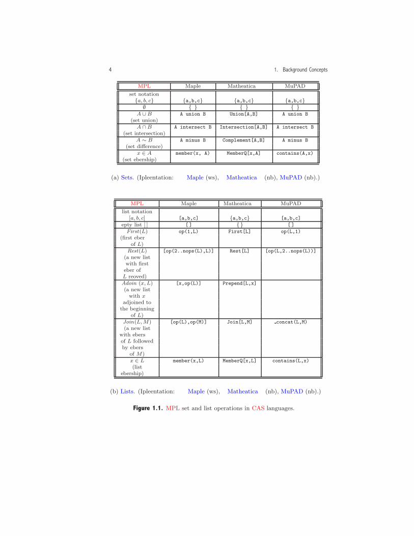
The MPL set and list operators and the corresponding operators incomputer algebra systems are given in Figure 1.1.
MPL mathematical expressions have two (somewhat overlapping) rolesas either program statements that represent a computational step in a pro-gram or as data objects that are processed by program statements.
Assignments, Functions, and Procedures
The MPL assignment operator is a colon followed by an equal sign (:=) andan assignment statement has the form f := u where u is a mathematicalexpression.
An MPL function definition has the form f(x1, . . . , xl)function:= u, where
x1, . . . , xl is a sequence of symbols called the formal parameters, and u isa mathematical expression. MPL procedures extend the function conceptto mathematical operators that are defined by a sequence of statements.The general form of an MPL procedure is given in Figure 1.2. Functionsand procedures are invoked with an expression of the form f(a1, . . . , al),where a1, . . . , al is a sequence of mathematical expressions called the actualparameters.
In order to promote a programming style that works for all languages,we adopt the following conventions for the use of local variables and formalparameters in a procedure:
• An unassigned local variable cannot appear as a symbol in a math-ematical expression. In situations where a procedure requires a lo-cal (unassigned) mathematical symbol, we either pass the symbolthrough the parameter list or use a global symbol.
• Formal parameters are used only to transmit data into a procedureand not as local variables or to return data from a procedure. Whenwe need to return more than one expression from a procedure, wereturn a set or list of expressions.
Decision and Iteration Structures
MPL provides three decision structures: the if structure, the if-else struc-ture which allows for two alternatives, and the multi-branch decision struc-ture which allows for a sequence of alternatives.
MPL contains two iteration structures that allow for repeated evalua-tion of a sequence of statements, the while structure and the for structure.Some of our procedures contain for loops that include a Return statement.
4 1. Background Concepts
MPL Maple Mathematica MuPAD
set notation{a, b, c} {a,b,c} {a,b,c} {a,b,c}
∅ { } { } { }A ∪ B A union B Union[A,B] A union B
(set union)A ∩ B A intersect B Intersection[A,B] A intersect B
(set intersection)A ∼ B A minus B Complement[A,B] A minus B
(set difference)x ∈ A member(x, A) MemberQ[x,A] contains(A,x)
(set membership)
(a) Sets. (Implementation: Maple (mws), Mathematica (nb), MuPAD (mnb).)
MPL Maple Mathematica MuPAD
list notation[a, b, c] [a,b,c] {a,b,c} [a,b,c]
empty list [ ] [ ] { } [ ]
First(L) op(1,L) First[L] op(L,1)
(first memberof L)Rest(L) [op(2..nops(L),L)] Rest[L] [op(L,2..nops(L))]
(a new listwith first
member ofL removed)Adjoin(x, L) [x,op(L)] Prepend[L,x] [x, op(L)]
(a new listwith x
adjoined tothe beginning
of L)Join(L, M) [op(L),op(M)] Join[L,M] concat(L,M)
(a new listwith membersof L followedby members
of M)x ∈ L member(x,L) MemberQ[x,L] contains(L,x)
(listmembership)
(b) Lists. (Implementation: Maple (mws), Mathematica (nb), MuPAD (mnb).)
Figure 1.1. MPL set and list operations in CAS languages.

1.3. Automatic Simplification and Expression Structure 5
Procedure f(x1, . . . , xl);Input
x1 : description of input to x1;...
xl : description of input to xl;Output
description of output;Local Variables
v1, . . . , vm;Begin
S1;...Sn
End
Figure 1.2. The general form of an MPL procedure. (Implementation: Maple(txt), Mathematica (txt), MuPAD (txt).)
In this case, we intend that both the loop and the procedure terminatewhen the Return is encountered.1
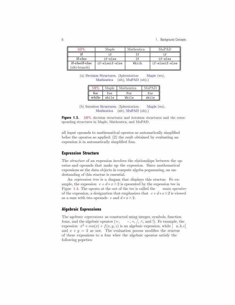
All computer algebra languages provide decision and iteration struc-tures (Figure 1.3).
1.3 Automatic Simplification and Expression Structure
As part of the evaluation process, computer algebra systems apply some“obvious” simplification rules from algebra and trigonometry that removeextraneous symbols from an expression and transform it to a standard form.This process is called automatic simplification. For example,
x+ 2 x+ y y2 + z0 + sin(π/4)→ 3 x+ y3 + 1 +√2/2
where the expression to the right of the arrow gives the automaticallysimplified form after evaluation.
In MPL (as in a CAS), all expressions in dialogues and computer pro-grams operate in the context of automatic simplification. This means: (1)
1 The for statements in both Maple and MuPAD work in this way. However, inMathematica, a Return in a For statement will only work in this way if the upper limitcontains a relational operator (e.g., i<=N). (Implementation: Mathematica (nb).)
6 1. Background Concepts
MPL Maple Mathematica MuPAD
if if If if
if-else if-else If if-else
if-elseif-else if-elseif-else Which if-elseif-else
(multi-branch)
(a) Decision Structures. (Implementation: Maple (mws),Mathematica (nb), MuPAD (mnb).)
MPL Maple Mathematica MuPAD
for for For for
while while While while
(b) Iteration Structures. (Implementation: Maple (mws),Mathematica (nb), MuPAD (mnb).)
Figure 1.3. MPL decision structures and iteration structures and the corre-sponding structures in Maple, Mathematica, and MuPAD.
all input operands to mathematical operators are automatically simplifiedbefore the operators are applied; (2) the result obtained by evaluating anexpression is in automatically simplified form.
Expression Structure
The structure of an expression involves the relationships between the op-erators and operands that make up the expression. Since mathematicalexpressions are the data objects in computer algebra programming, an un-derstanding of this structure is essential.
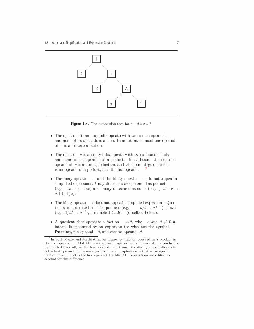
An expression tree is a diagram that displays this structure. For ex-ample, the expression c+ d ∗ x ∧ 2 is represented by the expression tree inFigure 1.4. The operator at the root of the tree is called the main operatorof the expression, a designation that emphasizes that c+ d ∗x∧ 2 is viewedas a sum with two operands c and d ∗ x ∧ 2.
Algebraic Expressions
The algebraic expressions are constructed using integers, symbols, functionforms, and the algebraic operators (+, −, ∗, /, ∧, and !). For example, theexpression x2 + cos(x) + f(x, y, z) is an algebraic expression, while [a, b, c]and x + y = 2 are not. The evaluation process modifies the structureof these expressions to a form where the algebraic operators satisfy thefollowing properties:
1.3. Automatic Simplification and Expression Structure 7
❅❅
❅❅
��
��
❅❅
��
x
d
+
c ∗
∧
2
Figure 1.4. The expression tree for c + d ∗ x ∧ 2.
• The operator + is an n-ary infix operator with two or more operandsand none of its operands is a sum. In addition, at most one operandof + is an integer or fraction.
• The operator ∗ is an n-ary infix operator with two or more operandsand none of its operands is a product. In addition, at most oneoperand of ∗ is an integer or fraction, and when an integer or fractionis an operand of a product, it is the first operand.2
• The unary operator − and the binary operator − do not appear insimplified expressions. Unary differences are represented as products(e.g. −x → (−1)x) and binary differences as sums (e.g. (a − b →a+ (−1) b).
• The binary operator / does not appear in simplified expressions. Quo-tients are represented as either products (e.g., a/b → a b−1), powers(e.g., 1/a2 → a−2), or numerical fractions (described below).
• A quotient that represents a fraction c/d, where c and d �= 0 areintegers is represented by an expression tree with root the symbolfraction, first operand c, and second operand d.
2In both Maple and Mathematica, an integer or fraction operand in a product isthe first operand. In MuPAD, however, an integer or fraction operand in a product isrepresented internally as the last operand even though the displayed form indicates itis the first operand. Since some algorithms in later chapters assume that an integer orfraction in a product is the first operand, the MuPAD implementations are modified toaccount for this difference.

8 1. Background Concepts
❅❅
❅❅
��
❅❅
��
✟✟✟✟❍❍❍❍
✟✟✟✟❍❍❍❍
−
/
∗ 3
x y
3−1
yx
∗
fraction
unsimplified simplified
Figure 1.5. Expression trees for −x ∗ y/3 and its simplified form (−1/3) ∗ x ∗ y.
• For u = v∧n, where n is an integer, the expression v is not an integer,fraction, product, or power (e.g., (x2)3 → x6).
• The operand of ! is not a non-negative integer (e.g., 3!→ 6).
Figure 1.5 shows the expression trees for the expression −x ∗ y/3 and itssimplified form ((−1)/3)∗x∗y. Observe that in simplified form, the operator∗ is an n-ary operator with three operands, the − is part of the integer −1,and the fraction (−1)/3 has main operator fraction.
The structure of algebraic expressions is described in detail in Cohen[24], Chapter 3. Non-algebraic expressions include relational and logical ex-pressions, lists, and sets. The structure of these expressions in a particularCAS can be determined using the primitive operators in Figure 1.6.
Primitive Operators for Simplified Mathematical Expressions
MPL uses four primitive operators to access the structure of expressionsand to construct expressions.
• Kind(u). This operator returns the type of expression (e.g., symbol,integer, fraction, +, ∗, ∧, !, =, <, ≤, >, ≥, �=, and, or, not, set,list, and function names). For example, Kind(m ∗ x+ b)→ +.
• Number of operands(u). This operator returns the number of operandsof the main operator of u. For example,
Number of operands(a ∗ x+ b ∗ x+ c)→ 3.

1.3. Automatic Simplification and Expression Structure 9
• Operand(u, i). This operator returns the ith operand of the mainoperator of u. For example, Operand(m ∗ x+ b, 2)→ b.
• Construct(f, L). Let f be an operator (+, ∗, =, etc.) or a symbol,and let L = [a, b, . . . , c] be a list of expressions. This operator returnsan expression with main operator f and operands a, b, . . . , c. Forexample, Construct(” + ”, [a, b, c])→ a+ b + c.
The primitive operators in computer algebra systems are given in Figure1.6(a). Although Mathematica has an operator that constructs expressions,Maple and MuPAD do not. However, in both of these languages, theoperation can be simulated with a procedure. (Implementation: Maple(txt), MuPAD (txt).)
MPL Maple Mathematica MuPAD
Kind(u) whattype(u) Head(u) type(u)
and andop(0,u) op(u,0)
for function for undefinednames function names
Operand(u, i) op(i,u) Part[u,i] op(u,i)
and Numerator[u]
and Denominator[u]
for fractionsNumber of operands(u) nops(u) Length[u] nops(u)
Construct(f, L) (simulated Apply[f,L] (simulatedwith a with a
procedure) procedure)
(a) Primitive Structural Operators. (Implementation: Maple (mws),
Mathematica (nb), MuPAD (mnb).)
MPL Maple Mathematica MuPAD
Free of(u, t) not(has(u,t)) FreeQ[u,x] not(has(u,t))
Substitute(u, subs(t=r,u) ReplaceAll[u,t->r] subs(u,t=r)
t=r) oru/.t->r
(b) Structure-based Operators. (Implementation: Maple (mws),
Mathematica (nb), MuPAD (mnb).)
Figure 1.6. Operators in Maple, Mathematica, and MuPAD that are mostsimilar to MPL’s primitive structural operators and structure-based operators.
10 1. Background Concepts
Structure-Based Operators
A complete sub-expression of an automatically simplified expression u iseither the expression u itself or an operand of some operator in u. Interms of expression trees, the complete sub-expressions of u are either theexpression tree for u or one of its sub-trees. For example, for a∗ (1+ b+ c),the expression 1 + b+ c is a complete sub-expression while 1 + b is not.
The next two MPL operators are based only on the structure of anexpression.
• Free of(u, t). Let u and t (for target) be mathematical expressions.This operator returns false when t is identical to some complete sub-expression of u and otherwise returns true. For example,
Free of ((a+ b) c, a+ b)→ false.
• Substitute(u, t = r). Let u, t, and r be mathematical expressions.This operator forms a new expression with each occurrence of thetarget expression t in u replaced by the replacement expression r. Thesubstitution occurs whenever t is structurally identical to a completesub-expression of u. For example,
Substitute((a+ b) c, a+ b = x)→ x c.
The operators in computer algebra systems that are most similar to MPL’sstructure-based operators are given in Figure 1.6(b).
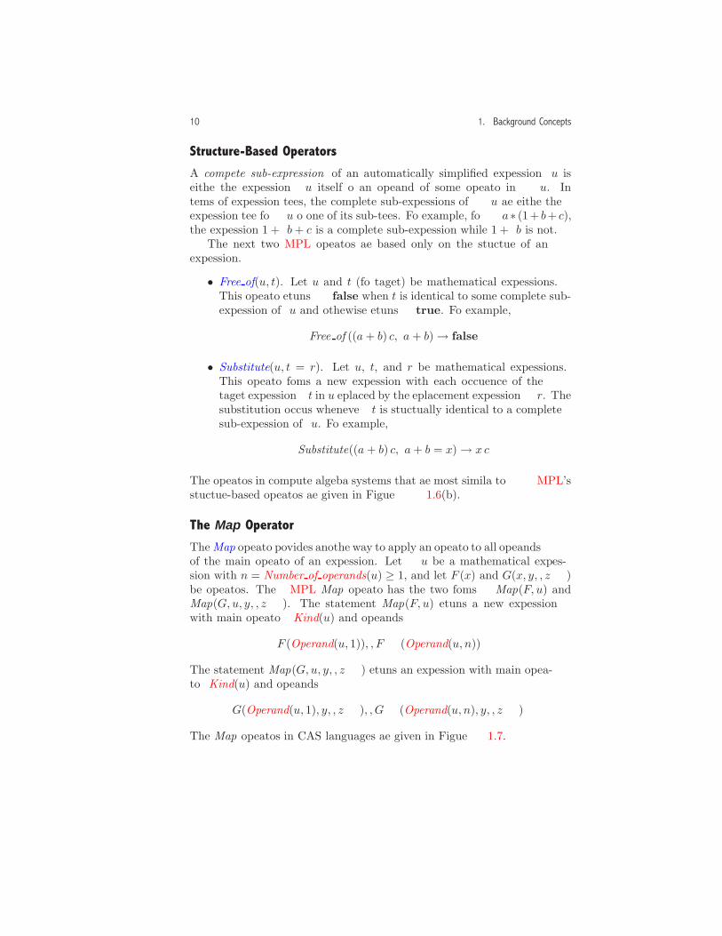
The Map OperatorTheMap operator provides another way to apply an operator to all operandsof the main operator of an expression. Let u be a mathematical expres-sion with n = Number of operands(u) ≥ 1, and let F (x) and G(x, y, . . . , z)be operators. The MPL Map operator has the two forms Map(F, u) andMap(G, u, y, . . . , z). The statement Map(F, u) returns a new expressionwith main operator Kind(u) and operands
F (Operand(u, 1)), . . . , F (Operand(u, n)).
The statement Map(G, u, y, . . . , z) returns an expression with main opera-tor Kind(u) and operands
G(Operand(u, 1), y, . . . , z), . . . , G(Operand(u, n), y, . . . , z).
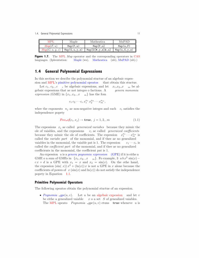
The Map operators in CAS languages are given in Figure 1.7.
1.4. General Polynomial Expressions 11
MPL Maple Mathematica MuPAD
Map(F, u) Map(F,u) Map[F,u] Map(u,F)
Map(G,u, y, z) Map(G,u,y,z) Map[G[#,y,z]&,u] Map(u,G,y,z)
Figure 1.7. The MPL Map operator and the corresponding operators in CASlanguages. (Implementation: Maple (mws), Mathematica (nb), MuPAD (mnb).)
1.4 General Polynomial Expressions
In this section we describe the polynomial structure of an algebraic expres-sion and MPL’s primitive polynomial operators that obtain this structure.
Let c1, c2, . . . , cr be algebraic expressions, and let x1,x2,. . . ,xm be al-gebraic expressions that are not integers or fractions. A general monomialexpression (GME) in {x1, x2, . . . , xm} has the form
c1 c2 · · · cr xn11 xn2
2 · · ·xnmm ,
where the exponents nj are non-negative integers and each ci satisfies theindependence property
Free of(ci, xj)→ true, j = 1, 2, . . . ,m. (1.1)
The expressions xj are called generalized variables because they mimic therole of variables, and the expressions ci are called generalized coefficientsbecause they mimic the role of coefficients. The expression xn1
1 · · ·xnmm is
called the variable part of the monomial, and if there are no generalizedvariables in the monomial, the variable part is 1. The expression c1 · · · cr iscalled the coefficient part of the monomial, and if there are no generalizedcoefficients in the monomial, the coefficient part is 1.
An expression u is a general polynomial expression (GPE) if it is either aGME or a sum of GMEs in {x1, x2, . . . , xm}. For example, 3 a b x2 sin(x)−c x + d is a GPE with x1 = x and x2 = sin(x). On the other hand,the expression (sin(x))x2 + (ln(x))x is not a GPE in x alone because thecoefficients of powers of x (sin(x) and ln(x)) do not satisfy the independenceproperty in Equation 1.1.
Primitive Polynomial Operators
The following operators obtain the polynomial structure of an expression.
• Polynomial gpe(u, v). Let u be an algebraic expression and let vbe either a generalized variable x or a set S of generalized variables.The MPL operator Polynomial gpe(u, v) returns true whenever u is

12 1. Background Concepts
a GPE in {x} or in S, and otherwise returns false. For example,Polynomial gpe(x2 + y2, {x, y})→ true.
• Degree gpe(u, x). Let u = c1 · · · cr · xn11 · · ·xnm
m be a monomial withnon-zero coefficient part. The degree of u with respect to xi is de-noted by deg(u, xi) = ni. By mathematical convention, the degree ofthe 0 monomial is−∞. If u is a GPE in xi that is a sum of monomials,then deg(u, xi) is the maximum of the degrees of the monomials. Ifthe generalized variable xi is understood from context, we use the sim-pler notation deg(u). The MPL operator Degree gpe(u, x) returnsdeg(u, x). For example, Degree gpe(sin2(x)+b sin(x)+c, sin(x))→ 2.
• Coefficient gpe(u, x, j). Let u be a GPE in x, and let j be a non-negative integer. The MPL operator Coefficient gpe(u, x, j) returnsthe sum of the coefficient parts of all monomials of u with variablepart xj . For example, Coefficient gpe(a x+ b x+ y, x, 1)→ a+ b.
• Leading coefficient gpe(u, x). Let u be a GPE in x. The leadingcoefficient of a GPE u �= 0 with respect to x is the sum of the coef-ficient parts of all monomials with variable part xdeg(u,x). The zeropolynomial has, by definition, leading coefficient zero. The leadingcoefficient is represented by lc(u, x), and when x is understood fromcontext by lc(u). The MPL operator Leading coefficient gpe(u, x) re-turns lc(u, x). For example, Leading coefficient gpe(a x+b x+y, x)→a+ b.
• Variables(u). The polynomial structure of an algebraic expression udepends on which expressions are chosen as the generalized variables.The MPL operator Variables(u) selects a set of generalized variablesso that the coefficients of all monomials in u are rational numbers.For example, Variables(4x3 + 3x2 sin(x))→ {x, sin(x)}.
The operators in computer algebra languages that are most similar toMPL’s polynomial operators are given in Figure 1.8.
1.5 Miscellaneous Operators
Some additional MPL operators that are used in our algorithms and ex-ercises are given in Figure 1.9. Many more operators are defined in laterchapters.

1.5.Miscellaneous
Operators13
MPL Maple Mathematica MuPAD
Polynomial gpe(u, x) type(u,polynom(anything,x)) PolynomialQ[u,x] testtype(u, Type::PolyExpr(x))
Degree gpe(u, x) degree(u,x) Exponent[u,x] degree(u,x)
Coefficient gpe(u, x, n) coeff(u,x,n) Coefficient[u,x,n] coeff(u,x,n)
Leading coefficient gpe(u, x, n) lcoeff(u,x) Coefficient[u,x, lcoeff(u,x)
Exponent[u,x]]
Variables(u) indets(u) Variables[u] indets(u,PolyExpr)
Figure 1.8. The polynomial operators in Maple, Mathematica, and MuPAD that are most similar to those in MPL. (Imple-mentation: Maple (mws), Mathematica (nb), MuPAD (mnb).)

14 1. Background Concepts
MPL Maple Mathematica MuPAD
Return(u) RETURN(u) Return[u] return(u)
Operand list(u) [op(u)] Apply[List,u] [op(u)]
Absolute value(u) abs(u) Abs[u] abs(u)
|u|Max({n1, . . . , nr}) max(n1, . . . , nr) Max[n1, . . . , nr] max(n1, . . . , nr)
Algebraic expand(u) expand(u) Expand[u] expand(u)
Numerator(u) numer(u) Numerator[u] numer(u)
Denominator(u) denom(u) Denominator[u] denom(u)
Derivative(u, x) diff(u, x) D[u, x] diff(u, x)
Figure 1.9. Miscellaneous operators. (Implementation: Maple (mws),Mathematica (nb), MuPAD (mnb).)
Further Reading
1.1 Computer Algebra Systems. Additional information on computer alge-bra can be found in Akritas [2], Buchberger et al. [17], Davenport, Siret, andTournier [29], Geddes, Czapor, and Labahn [39],Lipson [64], Mignotte [66],Mignotte and Stefanescu [67], Mishra [68], von zur Gathen and Gerhard [96],Wester [100], Winkler [101], Yap [105], and Zippel [108]. Two older (but in-teresting) discussions of computer algebra are found in Pavelle, Rothstein, andFitch [77] and Yun and Stoutemyer [107]. Simon ([89], and [90]), Wester [100](Chapter 3), and the web site
http://math.unm.edu/~wester/cas_review.html
give comparisons of commercial computer algebra software. Information aboutcomputer algebra and computer algebra systems can be found at the web sites:
• SymbolicNet: http://www.SymbolicNet.org.
• Computer Algebra Information Network (CAIN):http://www.riaca.win.tue.nl/CAN/
• COMPUTER ALGEBRA, Algorithms, Systems and Applications:http://www-troja.fjfi.cvut.cz/~liska/ca/
• sci.math.symbolic:http://mathforum.org/discussions/about/sci.math.symbolic.html
The Association for Computing Machinery (ACM) has a Special Interest Groupon Symbolic and Algebraic Manipulation (SIGSAM). This group publishes a quar-terly journal the SIGSAM Bulletin which provides a forum for exchanging ideasabout computer algebra. In addition, SIGSAM sponsors an annual conference,the International Symposium on Symbolic and Algebraic Computation (ISSAC).Information about SIGSAM is found at http://www.acm.org/sigsam. The mainresearch journal in computer algebra is the Journal of Symbolic Computation(http://www.academicpress.com/jsc).

1.5. Miscellaneous Operators 15
1.2 Mathematical Pseudo-language (MPL). The basic elements of MPL aredescribed in Cohen [24], Chapter 2, and the basic concepts in computer algebraprogramming are described in Chapters 4 and 5.
1.3 Automatic Simplification and Expression Structure. The evaluationprocess and the structure of expressions is described in greater detail in Cohen[24], Chapter 3, and an algorithm for the Free of operator is given in Chapter 5.
1.4 General Polynomial Expressions. Algorithms for the operators in thissection are given in Cohen [24], Chapter 6.
1.5 Miscellaneous Operators. Cohen [24] has algorithms for Algebraic expand ,
Numerator , and Denominator (Chapter 6), and Derivative (Chapter 5).

2
Integers, Rational Numbers,and Fields
The chapter is concerned with the numerical objects that arise in computeralgebra including the integers, the rational numbers, and other classes ofnumerical expressions. In Section 2.1 we discuss the basic mathematicalproperties of the integers and describe some algorithms that are importantfor computer algebra. Section 2.2 is concerned with the manipulation ofrational numbers. We define a standard form for a rational number anddescribe an algorithm that evaluates involved arithmetic expressions withintegers and fractions to a rational number in standard form. In Section 2.3we introduce the concept of a field, which is a mathematical system withaxioms that describe in a general way the algebraic properties of the ratio-nal numbers and other classes of expressions that arise in computer algebra.We give a number of examples of fields and show that many transformationsthat are routinely used in the manipulation of mathematical expressionsare logical consequences of the field axioms.
2.1 The Integers
In this section we describe some mathematical and computational proper-ties of the integers
Z = {. . .− 2,−1, 0, 1, 2, . . .}.
17

18 Integers, Rational Numbers, and Fields
The following theorem gives the basic division property of the integers.1
Theorem 2.1. For integers a and b �= 0, there are unique integers q and rsuch that
a = q b+ r (2.1)
and0 ≤ r ≤ |b| − 1. (2.2)
The integer q is the quotient and is represented by the operator iquot(a, b)(for integer quotient). The integer r is the remainder and is representedby irem(a, b).
Example 2.2.
8 = q · 3 + r = 2 · 3 + 2,8 = q · (−3) + r = (−2) · (−3) + 2, (2.3)−8 = q · 3 + r = (−3) · 3 + 1, (2.4)−8 = q · (−3) + r = 3 · (−3) + 1. (2.5)
�
In Theorem 2.1, the quotient and remainder are chosen so that r ≥ 0.Another possibility is to choose the quotient and remainder so that
|r| ≤ |b| − 1, r · a ≥ 0. (2.6)
In this case, Equations (2.4) and (2.5) have the form
−8 = q · 3 + r = (−2) · 3− 2,−8 = q · (−3) + r = 2 · (−3)− 2.
A third possibility is to choose the quotient and remainder so that
|r| ≤ |b| − 1, r · b ≥ 0. (2.7)
In this case, Equations (2.3) and (2.5) have the form
8 = q · (−3) + r = (−3) · (−3)− 1,−8 = q · (−3) + r = 2 · (−3)− 2.
Most computer algebra languages have operators similar to iquot and irem,although the remainder may satisfy either property (2.6) or (2.7) insteadof (2.2) (see Figure 2.1).
1A proof of the theorem based on the formal axioms of the integers is given in Dean[31], pages 10–11.
2.1. The Integers 19
MPL Maple Mathematica MuPAD
iquot(a, b), (2.2) iquo(a, b), (2.6) Quotient[a, b], iquo(a, b), (2.6)(2.7) a div b, (2.2)
irem(a, b), (2.2) irem(a, b), (2.6) Mod[a, b], (2.7) irem(a, b), (2.6)a mod b, (2.2) a mod b, (2.2)
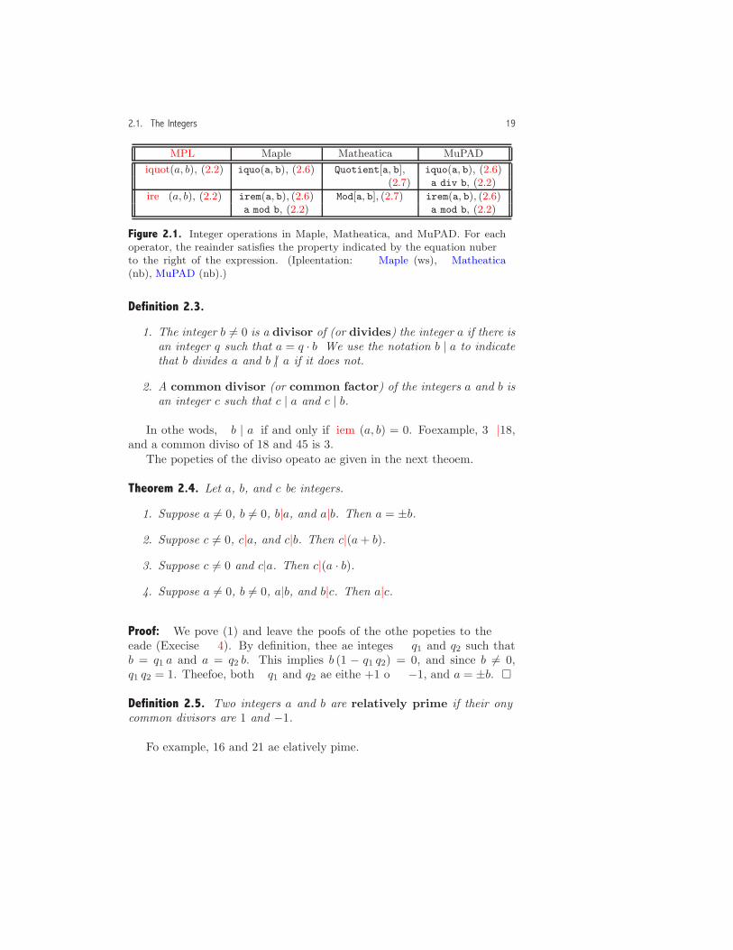
Figure 2.1. Integer operations in Maple, Mathematica, and MuPAD. For eachoperator, the remainder satisfies the property indicated by the equation numberto the right of the expression. (Implementation: Maple (mws), Mathematica(nb), MuPAD (mnb).)
Definition 2.3.
1. The integer b �= 0 is a divisor of (or divides) the integer a if there isan integer q such that a = q · b. We use the notation b | a to indicatethat b divides a and b /| a if it does not.
2. A common divisor (or common factor) of the integers a and b isan integer c such that c | a and c | b.
In other words, b | a if and only if irem(a, b) = 0. For example, 3|18,and a common divisor of 18 and 45 is 3.
The properties of the divisor operator are given in the next theorem.
Theorem 2.4. Let a, b, and c be integers.
1. Suppose a �= 0, b �= 0, b|a, and a|b. Then a = ±b.2. Suppose c �= 0, c|a, and c|b. Then c|(a+ b).
3. Suppose c �= 0 and c|a. Then c|(a · b).4. Suppose a �= 0, b �= 0, a|b, and b|c. Then a|c.
Proof: We prove (1) and leave the proofs of the other properties to thereader (Exercise 4). By definition, there are integers q1 and q2 such thatb = q1 a and a = q2 b. This implies b (1 − q1 q2) = 0, and since b �= 0,q1 q2 = 1. Therefore, both q1 and q2 are either +1 or −1, and a = ±b. �
Definition 2.5. Two integers a and b are relatively prime if their onlycommon divisors are 1 and −1.
For example, 16 and 21 are relatively prime.

20 Integers, Rational Numbers, and Fields
Greatest Common Divisors
The greatest common divisor of two integers a and b is the largest (non-negative) common divisor of a and b. Although this description is intu-itively appealing, a more formal definition is helpful for the developmentof an algorithm.
Definition 2.6. Let a and b be integers. The greatest common divisor (gcd)of a and b (at least one of which is non-zero) is an integer d that satisfiesthe following three properties:
1. d is a common divisor of a and b.
2. If e is another common divisor of a and b, then e|d.
3. d > 0.
The notation gcd(a, b) denotes the greatest common divisor.If both a = 0 and b = 0, the above definition does not apply. In this
case, by definition, gcd(0, 0) = 0.
Property 2 is a roundabout way of saying that d is the largest commondivisor of a and b.
Example 2.7.
gcd(24, 18) = 6,gcd(−24, 18) = 6,
gcd(34, 0) = 34,gcd(17, 23) = 1.
Let’s formally verify that gcd(24, 18) = d = 6 using Definition 2.6. Sinceproperties (a) and (c) are obviously true, we need only verify (b). Dividing24 by 18, we have 24 = 1 · 18+ 6, and so, by Theorem 2.4(2), any commondivisor e of 24 and 18 also divides d. �
The greatest common divisor is used to reduce a fraction to lowestterms. For example, to reduce 18/24, we have gcd(18, 24) = 6, and dividethe numerator and denominator by the gcd to obtain 3/4.
The next theorem gives three important properties of the greatest com-mon divisor.
2.1. The Integers 21
Theorem 2.8. Let a and b be integers. Then,
1. gcd(a, b) exists;
2. gcd(a, b) is unique;
3. gcd(b, 0) = |b|.
Proof: While Part (1) may appear obvious from the intuitive idea of agreatest common divisor, it is included here to emphasize that we shouldnot simply assume that there is an integer d that satisfies the second prop-erty in Definition 2.6. We omit the proof of this fact, but note that thealgorithm that computes the gcd given later in this section implies thatthe gcd exists.2
To show Part (2), suppose either a �= 0 or b �= 0, and suppose d1 and d2
are both greatest common divisors. Property (2) in Definition 2.6 impliesd1|d2 and d2|d1, and so by Theorem 2.4(1), d1 = ±d2. Since d1 > 0 andd2 > 0, we have d1 = d2. If both a = 0 and b = 0, the gcd is unique bydefinition.
The proof of Part (3) is left to the reader (Exercise 12). �
Euclid’s Greatest Common Divisor Algorithm
A simple (but highly inefficient) approach for finding the gcd is to testall integers less than or equal to min({|a|, |b|}). A much more efficientalgorithm, which uses the remainders in integer division, is based on thenext theorem:
Theorem 2.9. Let a and b �= 0 be integers, and let r = irem(a, b). Then,
gcd(a, b) = gcd(b, r). (2.8)
Proof: Let d = gcd(b, r). We show that d is the gcd of a and b by showingthat it satisfies the three properties in Definition 2.6. The proof is basedon the relationship
a = q b+ r. (2.9)
First, since d|b and d|r, Theorem 2.4(2),(3) implies d|a, and so d satisfiesDefinition 2.6(1). Next, if e is any divisor of a and b, then Equation (2.9)implies e|r, and so e is a common divisor of b and r. Therefore, Defini-tion 2.6(2) (applied to b and r) implies e|d, which means Definition 2.6(2)
2A non-algorithmic proof that the gcd exits, which is based on the formal axioms ofthe integers, is given in Akritas [2], page 36.

22 Integers, Rational Numbers, and Fields
holds for a and b as well. Finally, since d is a gcd, it is positive, andDefinition 2.6(3) is satisfied. �
The gcd algorithm that is based on Equation (2.8) is known as Euclid’salgorithm. It is one of the earliest known numerical algorithms (about300 B.C.E.). When b �= 0, define a sequence of integers R−1, R0, R1, . . .with the scheme
R−1 = a,
R0 = b,
R1 = irem(R−1, R0),... (2.10)
Ri+1 = irem(Ri−1, Ri),...
The sequence (2.10) is called an integer remainder sequence. By Theo-rem 2.1,
0 ≤ · · · < Ri+1 < Ri < · · · < R1 ≤ |b| − 1, (2.11)
and so some member of the sequence is zero. Let Rρ be the first remainderthat is zero. By repeatedly applying Equation (2.8), we have
gcd(a, b) = gcd(R−1, R0)= gcd(R0, R1)
...= gcd(Rρ−1, Rρ)= gcd(Rρ−1, 0)= |Rρ−1|. (2.12)
Notice that we have included the absolute value operation in (2.12) eventhough the remainders in (2.11) are all non-negative. There are, however,two cases where the absolute value is needed. First, when b �= 0 and b|a,we have irem(a, b) = 0, and so the remainder sequence terminates withR1 = 0. Therefore,
gcd(a, b) = gcd(b, 0) = |b| = |R0|.The second case involves R0 = b = 0 which means there are no iterations,and so
gcd(a, b) = gcd(a, 0) = |a| = |R−1|.
2.1. The Integers 23
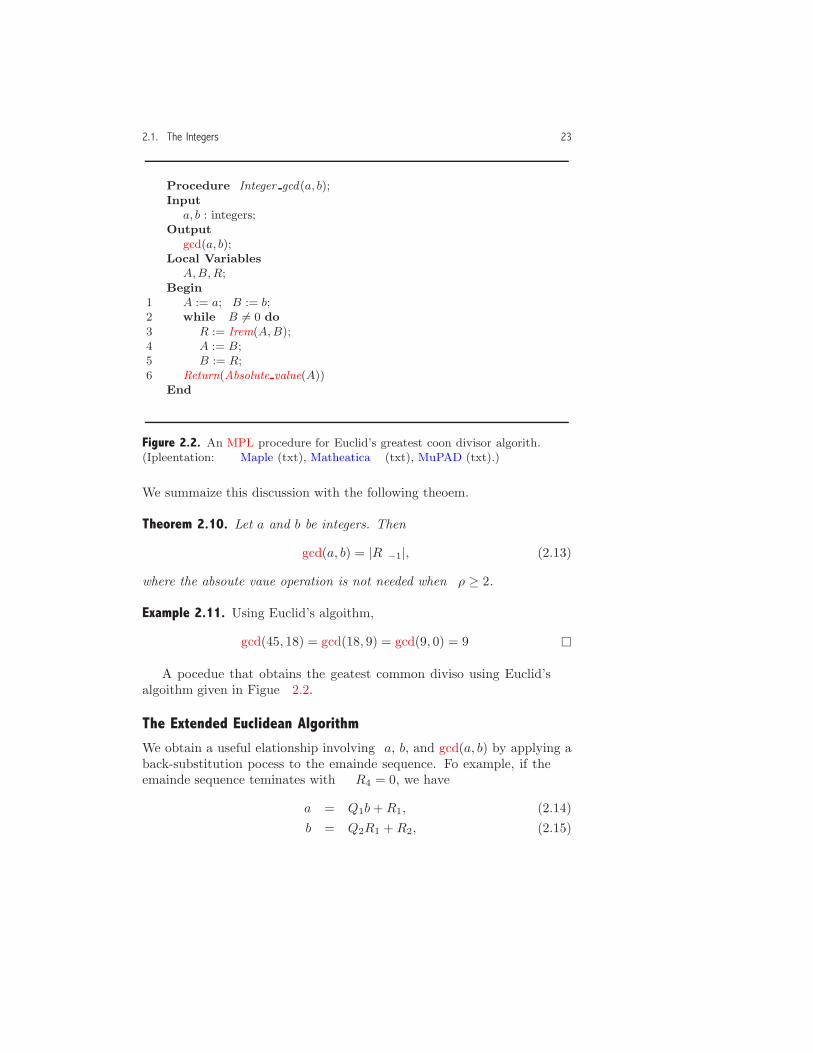
Procedure Integer gcd(a, b);Input
a, b : integers;Output
gcd(a, b);Local Variables
A,B,R;Begin
1 A := a; B := b;2 while B �= 0 do3 R := Irem(A,B);4 A := B;5 B := R;6 Return(Absolute value(A))
End
Figure 2.2. An MPL procedure for Euclid’s greatest common divisor algorithm.(Implementation: Maple (txt), Mathematica (txt), MuPAD (txt).)
We summarize this discussion with the following theorem.
Theorem 2.10. Let a and b be integers. Then
gcd(a, b) = |Rρ−1|, (2.13)
where the absolute value operation is not needed when ρ ≥ 2.
Example 2.11. Using Euclid’s algorithm,
gcd(45, 18) = gcd(18, 9) = gcd(9, 0) = 9. �
A procedure that obtains the greatest common divisor using Euclid’salgorithm given in Figure 2.2.
The Extended Euclidean Algorithm
We obtain a useful relationship involving a, b, and gcd(a, b) by applying aback-substitution process to the remainder sequence. For example, if theremainder sequence terminates with R4 = 0, we have
a = Q1b+R1, (2.14)b = Q2R1 +R2, (2.15)

24 Integers, Rational Numbers, and Fields
R1 = Q3R2 +R3, (2.16)R2 = Q4R3,
where Qi = iquot(Ri−2, Ri−1) and
gcd(a, b) = R3.
Using Equation (2.16) to substitute for R3 in this expression, we have
gcd(a, b) = R1 −Q3R2. (2.17)
Next, using Equations (2.14) and (2.15) to substitute for R1 and R2 inEquation (2.17), we obtain
gcd(a, b) = ma+ n b, (2.18)
wherem = 1 +Q2Q3, n = −Q1 −Q3 −Q1Q2Q3. (2.19)
This discussion suggests the following theorem.
Theorem 2.12. For integers a and b, there are integers m and n such that
ma+ n b = gcd(a, b).
A constructive proof of the theorem is given by an algorithm that com-putes m and n. (See the discussion following Theorem 2.14 and Equa-tion (2.27).)
Example 2.13. Let a = 45 and b = 18. The remainder sequence is
R−1 = 45, R0 = 18, R1 = 9, R2 = 0.
Therefore, since Q1 = 2,
gcd(45, 18) = |R1| = 9 = 45−Q1 · 18 = 1 · 45 + (−2) · 18,and so m = 1 and n = −2. �
An algorithm that obtains m and n along with gcd(a, b) is called theextended Euclidean algorithm and is simply a formalization of the back-substitution process. The algorithm is based on the following theorem.
Theorem 2.14. For integers a and b, there are integers mi and ni such that
mi a+ ni b = Ri, i = −1, 0, 1, ..., ρ.

2.1. The Integers 25
Proof: First, for i = −1 and i = 0,
R−1 = a = 1 · a+ 0 · b = m−1 a+ n−1 b, (2.20)R0 = b = 0 · a+ 1 · b = m0 a+ n0 b, (2.21)
and som−1 = 1, m0 = 0, (2.22)
andn−1 = 0, n0 = 1. (2.23)
Notice that Equations (2.20) and (2.21) include the case b = 0 becauseρ = 0 when this occurs. So let’s suppose b �= 0 which implies ρ ≥ 1.Consider the remainder sequence
a = R−1 = Q1R0 +R1,
b = R0 = Q2R1 +R2,
...Ri−2 = QiRi−1 +Ri, (2.24)
...
where Qi = iquot(Ri−2, Ri−1), Ri = irem(Ri−2, Ri−1), and the sequenceterminates when Rρ = 0. Using Equation (2.24), we derive a recurrencerelation for mi and ni:
Ri = Ri−2 −Qi Ri−1
= mi−2 a+ ni−2 b−Qi (mi−1 a+ ni−1 b)= (mi−2 −Qi mi−1) a+ (ni−2 −Qi ni−1) b. (2.25)
Therefore, since Ri = mi a+ ni b, we obtain the two recurrence relations
mi = mi−2 −Qi mi−1, ni = ni−2 −Qi ni−1. (2.26)
These recurrence relations, together with the initial conditions (2.22) and(2.23), give a scheme for computing the values mi and ni. �
Let’s return now to the computation of m and n. Since
gcd(a, b) = |Rρ−1|,
andRρ−1 = mρ−1a+ nρ−1b,

26 Integers, Rational Numbers, and Fields
Procedure Integer ext euc alg(a, b);Input
a, b : integers;Output
the list [gcd(a, b),m,n];Local Variablesmpp,mp, npp,np, A,B,Q,R,m, n;
Begin1 mpp := 1; mp := 0 ; npp := 0 ; np := 1 ; A := a; B := b;2 while B �= 0 do3 Q := Iquot(A,B);4 R := Irem(A,B);5 A := B; B := R;6 m = mpp − Q ∗mp; n := npp − Q ∗ np ;7 mpp := mp; mp := m; npp := np; np := n;8 if A ≥ 0 then9 Return([A, mpp, npp])10 else11 Return([−A, −mpp, − npp])
End
Figure 2.3. An MPL procedure for the extended Euclidean algorithm. (Imple-mentation: Maple (txt), Mathematica (txt), MuPAD (txt).)
we havem = ±mρ−1, n = ±nρ−1, (2.27)
where the plus signs apply when Rρ−1 ≥ 0 and the minus signs applyotherwise.
Example 2.15. Let a = 45 and b = 18. We have
Q1 = 2, R1 = 9, m1 = 1, n1 = −2,Q2 = 2, R2 = 0, m2 = −2, n2 = 5.
Therefore ρ = 2 and
gcd(45, 18) = |R1| = 9, m = m1 = 1, n = n1 = −2. �
A procedure that computes gcd(a, b) and the integers m and n from therecurrence relations (2.26) with initial conditions (2.22) and (2.23) is givenin Figure 2.3. The variables mp and np contain the previous values mi−1
and ni−1, and mpp and npp contain the values for mi−2 and ni−2.

2.1. The Integers 27
Theorem 2.12 is important for computer algebra in both a theoreticalsense and a computational sense. For example, the next theorem is basedon this theorem. Recall that an integer n > 1 is prime if its only positivedivisors are 1 and n.
Theorem 2.16. Suppose that a, b, and c are integers.
1. If c|(a b) and c and a are relatively prime, then c|b.2. If c|(a b) and c is prime, then c|a or c|b.3. If a|c, b|c, and gcd(a, b) = 1, then (a b)|c.
Proof: To prove (1), by Theorem 2.12 there are integers m and n suchthat mc+ n a = 1. Therefore
mc b+ n a b = b,
and since c divides each term in the sum on the left, c|b.To prove (2), if c /|a, then, since c is prime, c and a are relatively prime
and so by Part (1), c|b.To prove (3), let c = q1 a. Using Part (1), since b|(q1 a) and b and a are
relatively prime, we have b|q1. Therefore, q1 = q2 b, and c = q2 a b. �
Prime Factorization of Positive Integers
The following theorem is known as the Fundamental Theorem of Arith-metic.3
Theorem 2.17. An integer n > 1 can be factored uniquely as
n = pn11 · pn2
2 · · · pnss , (2.28)
where p1, p2, . . . , ps are prime numbers with pi < pi+1 and n1, n2, . . . ,nsare positive integers.
For example, 60 = 22 · 3 · 5.For large integers the factorization problem is computationally much
more difficult than the gcd problem. The references at the end of thechapter describe some approaches to this problem.
The prime factorization is obtained with the operator ifactor in bothMaple andMuPAD and the operator FactorInteger in Mathematica. (Im-plementation: Maple (mws), Mathematica (nb), MuPAD (mnb).)
3A proof of the theorem is given in Dean [31] pages 23–24. A similar proof for thefactorization of polynomials is given for Theorem 4.38 on page 138.
28 Integers, Rational Numbers, and Fields
The Chinese Remainder Problem
We conclude this section with a discussion of the Chinese remainder prob-lem, which is concerned with the solution of a system of integer remainderequations.
Definition 2.18. Let m1,m2, . . . ,mr be distinct positive integers that satisfy
gcd(mi,mj) = 1, for 1 ≤ i < j ≤ r. (2.29)
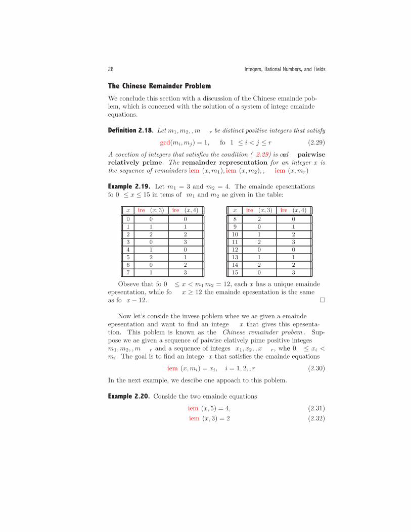
A collection of integers that satisfies the condition (2.29) is called pairwiserelatively prime. The remainder representation for an integer x isthe sequence of remainders irem(x,m1), irem(x,m2), . . . , irem(x,mr).
Example 2.19. Let m1 = 3 and m2 = 4. The remainder representationsfor 0 ≤ x ≤ 15 in terms of m1 and m2 are given in the table:
x irem(x, 3) irem(x, 4)
0 0 0
1 1 1
2 2 2
3 0 3
4 1 0
5 2 1
6 0 2
7 1 3
x irem(x, 3) irem(x, 4)
8 2 0
9 0 1
10 1 2
11 2 3
12 0 0
13 1 1
14 2 2
15 0 3
Observe that for 0 ≤ x < m1 m2 = 12, each x has a unique remainderrepresentation, while for x ≥ 12 the remainder representation is the sameas for x− 12. �
Now let’s consider the inverse problem where we are given a remainderrepresentation and want to find an integer x that gives this representa-tion. This problem is known as the Chinese remainder problem. Sup-pose we are given a sequence of pairwise relatively prime positive integersm1,m2, . . . ,mr and a sequence of integers x1, x2, . . . , xr, where 0 ≤ xi <mi. The goal is to find an integer x that satisfies the remainder equations
irem(x,mi) = xi, i = 1, 2, . . . , r. (2.30)
In the next example, we describe one approach to this problem.
Example 2.20. Consider the two remainder equations
irem(x, 5) = 4, (2.31)irem(x, 3) = 2. (2.32)

2.1. The Integers 29
We show that a solution is obtained with a sequence of divisions thatinvolves the remainder sequence (2.10) for 5 and 3 that is given by Euclid’salgorithm:
R−1 = 5, R0 = 3, R1 = 2, R2 = 1, R3 = 0.
First, observe that Equations (2.31) and (2.32) imply there are integers mand n such that
x = 5n+ 4 = 3m+ 2. (2.33)
Once we find the integers m and n so that both of these sums give thesame integer x, we will have a solution to the remainder equations. SolvingEquation (2.33) for m, we obtain
m =5n+ 2
3
= n+2n+ 2
3, (2.34)
where the last expression is obtained by dividing the denominator 3 (whichjust happens to be R0) into each of the coefficients of 5n+ 2. Since m isan integer, the fraction in Equation (2.34)
p =2n+ 2
3
must also reduce to an integer. Solving this equation for n we have
n =3 p− 2
2= p+
p
2− 1, (2.35)
where the last expression is obtained by dividing the denominator R1 = 2into each of the coefficients of 3 p− 2. Since n is an integer, the fraction inEquation (2.35) q =
p
2must also reduce to an integer. Therefore,
p = 2 q, (2.36)
and the process terminates since the denominator of 2 q is the remainderR2 = 1. At this point, we obtain a solution to Equation (2.33) by assign-ing q an integer value and obtaining integer values for p, n, and m usingEquations (2.36), (2.35), and (2.34). For example, if q = 1, we have p = 2,n = 2, m = 4 which gives solutions to Equation (2.33)
x = 5 · 2 + 4 = 3 · 4 + 2 = 14.
30 Integers, Rational Numbers, and Fields
Therefore, x = 14 is a solution to the remainder equations (2.31) and (2.32).Notice that there are infinitely many solutions to the remainder equationsbecause each integer q gives a distinct solution. �
The approach described in the last example gives an algorithm for thesolution of two remainder equations. The process terminates since m1 andm2 are relatively prime, and so some member of the remainder sequence isgcd(m1,m2) = 1. In Exercise 21 we describe a procedure that solves theChinese remainder problem using this approach.
Another approach to the Chinese remainder problem is based on theextended Euclidean algorithm. Let m1 and m2 be two relatively primepositive integers, and consider the remainder equations
irem(x,m1) = x1, (2.37)irem(x,m2) = x2, (2.38)
where 0 ≤ x1 < m1 and 0 ≤ x2 < m2. By the extended Euclideanalgorithm, there are integers c and d such that
cm1 + dm2 = 1. (2.39)
We use this relation to obtain a solution to the remainder equations. First,by multiplying both sides of this equation by x1 and rearranging we havedm2 x1 = (−c x1)m1 + x1, which implies
irem(dm2 x1, m1) = x1, irem(dm2 x1, m2) = 0. (2.40)
In other words, dm2 x1 is a solution to Equation (2.37) but not to Equation(2.38) (unless x2 = 0). In a similar way, by multiplying Equation (2.39) byx2, we obtain
irem(cm1x2, m2) = x2, irem(cm1x2, m1) = 0, (2.41)
which implies that cm1x2 is a solution to Equation (2.38) but not neces-sarily to Equation (2.37). However, the relations (2.40) and (2.41) suggestthat we can obtain a solution to both Equations (2.37) and (2.38) with thesum of the two partial solutions
w = cm1x2 + dm2x1. (2.42)
Indeed, using the relation in Exercise 1(a), we have
irem(w,m1) = irem(dm2 x1, m1) = x1,
irem(w,m2) = irem(cm1 x2, m2) = x2.

2.1. The Integers 31
Example 2.21. Let m1 = 5, m2 = 3, x1 = 4, and x2 = 2. Then, inEquation (2.39), c = −1 and d = 2, and from Equation (2.42), w = 14 is asolution to the remainder equations. �
In the next theorem and its proof, we describe a general solution andalgorithm for the Chinese remainder problem. The proof, which is similarto the above discussion, is based on the extended Euclidean algorithm.
Theorem 2.22. [Chinese Remainder Theorem] Let m1,m2, . . . ,mr be pos-itive integers that are pairwise relatively prime, and let x1, x2, . . . , xr beintegers with 0 ≤ xi < mi. Then, there is exactly one x in the interval
0 ≤ x < m1 ·m2 · · ·mr (2.43)
that satisfies the remainder equations
irem(x,mi) = xi, i = 1, 2, . . . , r. (2.44)
Proof: Observe that we obtain a unique solution by requiring that thesolution be in the interval (2.43). We show first that there is some solutionto the remainder equations (2.44) and then obtain a solution in this intervalusing integer division.
The proof is obtained with mathematical induction on the number ofequations r. For the base case r = 1, integer division shows that x = x1
is a solution to the first remainder equation. For the induction step, let’sassume there is an integer s that satisfies the remainder equations
irem(s,mi) = xi, i = 1, . . . , r − 1, (2.45)
and show how to extend the process one step further to find an integer wthat satisfies all of the remainder equations (2.44). Observe that Equation(2.45) implies
s = qimi + xi, i = 1, . . . , r − 1, (2.46)
where qi = iquot(s,mi). In addition, for
n = m1 · · ·mr−1, (2.47)
the condition (2.29) implies gcd(n,mr) = 1, and using the extended Eu-clidean algorithm, we obtain integers c and d such that
c n+ dmr = 1. (2.48)
Let
w = c n xr + dmr s, (2.49)m = m1 · · ·mr.
32 Integers, Rational Numbers, and Fields
We show that w satisfies all of the remainder equations. First, for 1 ≤ i ≤r − 1, we use Equation (2.48) to eliminate dmr from w to obtain
w = c n xr + (1− c n) s = (c n xr − c n s) + s. (2.50)
Using the equations (2.46) to eliminate the s on the far right, we obtain
w = (c n xr − c n s+ qimi) + xi.
Observe that by Equation (2.47), mi divides each of the terms in paren-theses, and therefore, the uniqueness property for integer division implies
irem(w,mi) = xi, 1 ≤ i ≤ r − 1.
For i = r, we use Equation (2.48) to eliminate c n from w to obtain
w = (dmr s− dmr xr) + xr.
Since mr divides each term in parentheses, the uniqueness property forinteger division implies irem(w,mr) = xr, and, therefore, w satisfies all ofthe remainder equations.
Although w satisfies all of the remainder equations, it may lie outsidethe 0 ≤ x < m. To obtain a solution in the interval, divide w by m toobtain w = q m + x, where 0 ≤ x < m. To show that x satisfies all theremainder equations, we have (using the relation in Exercise 1(a))
irem(x,mi) = irem(−q ·m+ w, mi)= irem((−q ·m1 · · ·mi−1 ·mi+1 · · ·mr)mi + w, mi)= irem(w,mi)= xi.
To show the uniqueness of the solution, suppose both x and x′ satisfythe conditions in the theorem. Then, for 1 ≤ i ≤ r we can represent x andx′ as
x = fimi + xi, x′ = gimi + xi
which implies (x− x′) = (fi− gi)mi. Therefore, mi|(x− x′), and since theintegers m1, . . . ,mr are relatively prime, Theorem 2.16(3) implies
m|(x− x′). (2.51)
However, since both x and x′ are positive and lie within the interval (2.43),we have −m < x − x′ < m. This inequality together with the condition(2.51) implies x = x′. �
2.1. The Integers 33
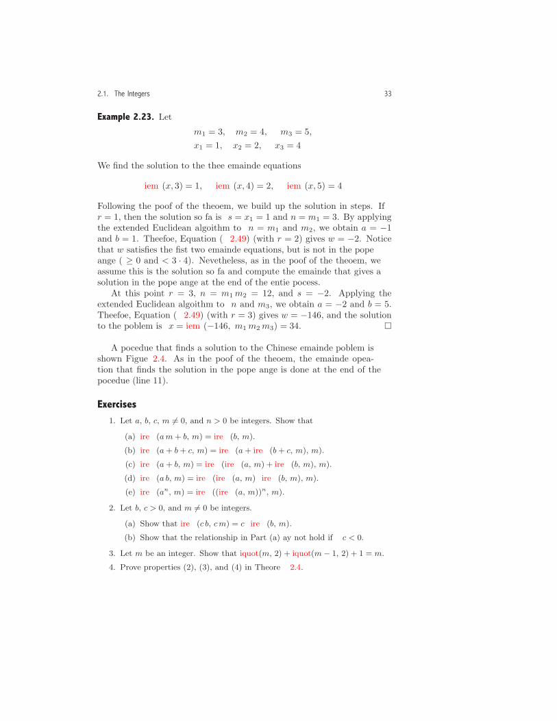
Example 2.23. Let
m1 = 3, m2 = 4, m3 = 5,x1 = 1, x2 = 2, x3 = 4.
We find the solution to the three remainder equations
irem(x, 3) = 1, irem(x, 4) = 2, irem(x, 5) = 4.
Following the proof of the theorem, we build up the solution in steps. Ifr = 1, then the solution so far is s = x1 = 1 and n = m1 = 3. By applyingthe extended Euclidean algorithm to n = m1 and m2, we obtain a = −1and b = 1. Therefore, Equation (2.49) (with r = 2) gives w = −2. Noticethat w satisfies the first two remainder equations, but is not in the properrange (≥ 0 and < 3 · 4). Nevertheless, as in the proof of the theorem, weassume this is the solution so far and compute the remainder that gives asolution in the proper range at the end of the entire process.
At this point r = 3, n = m1 m2 = 12, and s = −2. Applying theextended Euclidean algorithm to n and m3, we obtain a = −2 and b = 5.Therefore, Equation (2.49) (with r = 3) gives w = −146, and the solutionto the problem is x = irem(−146, m1 m2 m3) = 34. �
A procedure that finds a solution to the Chinese remainder problem isshown Figure 2.4. As in the proof of the theorem, the remainder opera-tion that finds the solution in the proper range is done at the end of theprocedure (line 11).
Exercises1. Let a, b, c, m �= 0, and n > 0 be integers. Show that
(a) irem(am + b, m) = irem(b, m).
(b) irem(a + b + c, m) = irem(a + irem(b + c, m), m).
(c) irem(a + b, m) = irem(irem(a, m) + irem(b, m), m).
(d) irem(a b, m) = irem(irem(a, m) · irem(b, m), m).
(e) irem(an, m) = irem((irem(a, m))n, m).
2. Let b, c > 0, and m �= 0 be integers.
(a) Show that irem(c b, cm) = c · irem(b, m).
(b) Show that the relationship in Part (a) may not hold if c < 0.
3. Let m be an integer. Show that iquot(m, 2) + iquot(m− 1, 2) + 1 = m.
4. Prove properties (2), (3), and (4) in Theorem 2.4.

34 Integers, Rational Numbers, and Fields
Procedure Chinese remainder(M,X);Input
M : a list of distinct pairwise relatively prime positive integers;X : a list of non-negative integers with
Number of operands(M) = Number of operands(X)and Operand(X, i) < Operand(M, i);
Outputthe solution described in Theorem 2.22;
Local Variablesn, s, i, x,m, e, c, d;
Begin1 n := Operand(M, 1);2 s := Operand(X, 1);3 for i from 2 to Number of operands(M) do4 x := Operand(X, i);5 m := Operand(M, i);6 e := Integer ext euc alg(n,m);7 c := Operand(e, 2);8 d := Operand(e, 3);9 s := c ∗ n ∗ x + d ∗m ∗ s;10 n := n ∗m;11 Return(Irem(s, n))
End
Figure 2.4. An MPL procedure that obtains the solution to the system of remain-der equations described in the Chinese remainder theorem. (Implementation:Maple (txt), Mathematica (txt), MuPAD (txt).)
5. Let u be a rational number. The floor of u (notation �u�) is the largestinteger ≤ u. The ceiling of u (notation �u�) is the smallest integer ≥ u.Give procedures Floor(u) and Ceiling(u) that performs these operations.Assume that the input expression u is an algebraic expression. When u isnot an integer or fraction, return the unevaluated form of the operators.
6. Give a procedure Integer divisors(n) that finds the positive and negativedivisors of an integer n �= 0. The result should be returned as a set or alist. For example,
Integer divisors(15) → {1,−1, 2,−2, 3,−3, 5,−5, 15,−15}.This exercise is used in the procedure Find S sets described in Exercise 5,page 369.
7. Let n be an integer. Give a procedure Number of digits(n) that returnsthe number of digits in n.
2.1. The Integers 35
8. Let n ≥ 0 and b ≥ 2 be integers. The integer n has a unique representationin the base b given by
n = b0 + b1 b + · · · + bk bk (2.52)
where 0 ≤ bi ≤ b− 1. For example, for b = 2,
5 = 1 + 0 · 2 + 1 · 22.
Give a procedure Base rep(n, b) that obtains this representation. Sinceautomatic simplification transforms the right side of Equation (2.52) ton, the procedure should return the representation as a list [b0, b1, . . . , bk],where bk �= 0. For n = 0, return the empty list [ ].
9. Give a recursive procedure for Euclid’s algorithm.
10. (a) Evaluate gcd(12768, 28424) using Euclid’s algorithm.
(b) Find integers m and n such that
m · 12768 + n · 28424 = gcd(12768, 28424).
11. The Fibonacci number sequence f0, f1, f2, . . . is defined using the recursivedefinition:
fj =1, when j = 0 or j = 1,fj−1 + fj−2, when j > 1.
For n ≥ 2, let R−1 = fn and R0 = fn−1 and consider the remaindersequence Ri in (2.10).
(a) Show that Ri = fn−(i+1) for i = −1, 0, . . . , ρ−1 and that the remain-der sequence terminates with ρ = n− 1 and gcd(fn, fn−1) = 1.
(b) For this sequence, what is the relation between mi and ni in theextended Euclidean algorithm and the Fibonacci numbers?
12. Prove Theorem 2.8(3).
13. Suppose that a, b, u, and v are integers and a = u gcd(a, b), b = v gcd(a, b).Show that gcd(u, v) = 1.
14. Suppose that gcd(a, b) = 1 and t is a positive integer. Show that
gcd(at, bt) = 1.
15. Let a, b, and c be integers. Show that
gcd(c a, c b) = |c| gcd(a, b).
16. Let a �= 0 and b �= 0 be integers. Show that a and b are relatively prime ifand only if there are integers m and n such that ma + n b = 1.
17. Give an example that shows that m and n in Theorem 2.12 are not unique.
18. Let a �= 0 and b �= 0 be integers, and define the least common multiple c ofa and b as follows:

36 Integers, Rational Numbers, and Fields
(a) a|c and b|c.(b) If a|d and b|d, then c|d.
(c) c > 0.
We use the notation lcm(a, b) to denote the least common multiple. Forexample, lcm(4, 6) = 12.
In this exercise, we derive the relation
lcm(a, b) =|a b|
gcd(a, b)(2.53)
using the following steps:
(a) Suppose that a|d, b|d, a = u gcd(a, b), and b = v gcd(a, b). Show thatthere is an integer r such that d = r u v gcd(a, b).
(b) Show that both a and b divide|a b|
gcd(a, b).
(c) Derive Equation (2.53).
In addition:
(d) Show that there are integers m and n such that lcm(a, b) = ma+n b.
(e) Give a procedure Integer lcm(a, b) that obtains lcm(a, b).
19. Solve each of the following systems of remainder equations.
(a) irem(x, 3) = 2, irem(x, 5) = 1, 0 ≤ x < 15.
(b) irem(x, 3) = 2, irem(x, 4) = 1, irem(x, 5) = 2, 0 ≤ x < 60.
20. Suppose that m1 = 4 and m2 = 6, and consider the remainder equations
irem(x, m1) = x1, irem(x, m2) = x2, 0 ≤ x < m1m2, (2.54)
where 0 ≤ x1 < m1 and 0 ≤ x2 < m2. (Notice that m1 and m2 are notrelatively prime.)
(a) Find x1 and x2 so that there is more than one solution to the equa-tions and inequality in (2.54).
(b) Find x1 and x2 so that the equations in (2.54) do not have a solution.
21. Let m > 0, n > 0, r, and s be integers with gcd(m,n) = 1. Give aprocedure Chinese remainder 2 (m, n, r, s) that obtains a solution to thetwo remainder equations irem(x, m) = r, irem(x, n) = s that is based onthe algorithm used in Example 2.20. The final solution should be in therange 0 ≤ x < mn. Do not use the extended Euclidean algorithm.

2.2. Rational Number Arithmetic 37
2.2 Rational Number Arithmetic
In a mathematical sense, a rational number is a fraction a/b where a andb �= 0 are integers. With this definition, each rational number can be rep-resented in infinitely many ways (e.g., 1/2 = 2/4 = (−2)/(−4), etc.). Theautomatic simplification process removes this ambiguity by transforming afraction to a standard form. Some typical examples4 are
2/4→ 1/2, 2/(−4)→ (−1)/2 (−2)/(−4)→ 1/2, 4/1→ 4.
These transformations suggest the following definition.
Definition 2.24. Let a and b be integers. An expression a/b is a fractionin standard form if it satisfies the following two properties:
1. b > 1.
2. gcd(a, b) = 1.
The fractions 2/3 and (-2)/3 are in standard form, while 4/6, 2/(−3),4/1, and 0/2 are not.
Each fraction can be transformed to either a fraction in standard formor an integer. This observation suggests the following definition.
Definition 2.25. An expression is a rational number in standard formif it is either a fraction in standard form or an integer.
The Simplify rational number OperatorLet u be an integer or a fraction with non-zero denominator. The operatorSimplify rational number(u) transforms u to a rational number in standardform (Figure 2.5). In order to bypass the automatic simplification processin a CAS (which transforms fractions to standard form), we represent thefraction a/b with the function notation FracOp(a, b) instead of the usualinfix notation.
Simplification of Rational Number Expressions
We consider next an algorithm that evaluates arithmetic expressions withintegers and fractions. The input to the algorithm is described in the nextdefinition.
4The displayed form of a fraction in a CAS may disguise the internal form.

38 Integers, Rational Numbers, and Fields
Procedure Simplify rational number (u);Input
u : a fraction in function (FracOp) notation (with non-zero denominator)or an integer;
Outputa fraction in standard form in function (FracOp) notation or an integer;
Local Variablesn, d, g;
Begin1 if Kind(u) = integer then Return(u)2 elseif Kind(u) = FracOp then3 n = Operand(u, 1);4 d = Operand(u, 2);5 if Irem(n, d) = 0 then Return(Iquot(n, d))6 else7 g := Integer gcd(n, d);8 if d > 0 then9 Return(FracOp(Iquot(n, g), Iquot(d, g)))10 elseif d < 0 then11 Return(FracOp(Iquot(−n, g), Iquot(−d, g)))
End
Figure 2.5. The MPL Simplify rational number procedure. (Implementation:Maple (txt), Mathematica (txt), MuPAD (txt).)
Definition 2.26. An algebraic expression u is a rational number expres-sion (RNE) if it satisfies one of the following rules:
RNE-1. u is an integer.
RNE-2. u is a fraction.
At this point, we allow for the possibility of a fraction with zero denomi-nator. The algorithm will recognize that such an expression is undefined.
RNE-3. u is a unary or binary sum with operands that are RNEs.
RNE-4. u is a unary or binary difference with operands that are RNEs.
RNE-5. u is a binary product with operands that are RNEs.
RNE-6. u is a quotient with operands that are RNEs.
RNE-7. u is a power with a base that is an RNE and an exponent that isan integer.
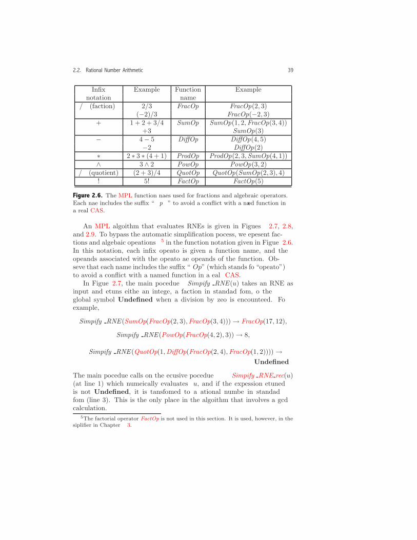
2.2. Rational Number Arithmetic 39
Infix Example Function Examplenotation name
/ (fraction) 2/3 FracOp FracOp(2, 3)(−2)/3 FracOp(−2, 3)
+ 1 + 2 + 3/4 SumOp SumOp(1, 2,FracOp(3, 4))+3 SumOp(3)
− 4− 5 DiffOp DiffOp(4, 5)−2 DiffOp(2)
∗ 2 ∗ 3 ∗ (4 + 1) ProdOp ProdOp(2, 3,SumOp(4, 1))∧ 3 ∧ 2 PowOp PowOp(3, 2)
/ (quotient) (2 + 3)/4 QuotOp QuotOp(SumOp(2, 3), 4)! 5! FactOp FactOp(5)
Figure 2.6. The MPL function names used for fractions and algebraic operators.Each name includes the suffix “Op” to avoid a conflict with a named function ina real CAS.
An MPL algorithm that evaluates RNEs is given in Figures 2.7, 2.8,and 2.9. To bypass the automatic simplification process, we represent frac-tions and algebraic operations5 in the function notation given in Figure 2.6.In this notation, each infix operator is given a function name, and theoperands associated with the operator are operands of the function. Ob-serve that each name includes the suffix “Op” (which stands for “operator”)to avoid a conflict with a named function in a real CAS.
In Figure 2.7, the main procedure Simplify RNE(u) takes an RNE asinput and returns either an integer, a fraction in standard form, or theglobal symbol Undefined when a division by zero is encountered. Forexample,
Simplify RNE (SumOp(FracOp(2, 3),FracOp(3, 4)))→ FracOp(17, 12),
Simplify RNE(PowOp(FracOp(4, 2), 3))→ 8,
Simplify RNE (QuotOp(1,DiffOp(FracOp(2, 4),FracOp(1, 2))))→Undefined.
The main procedure calls on the recursive procedure Simplify RNE rec(u)(at line 1) which numerically evaluates u, and if the expression returnedis not Undefined, it is transformed to a rational number in standardform (line 3). This is the only place in the algorithm that involves a gcdcalculation.
5The factorial operator FactOp is not used in this section. It is used, however, in thesimplifier in Chapter 3.
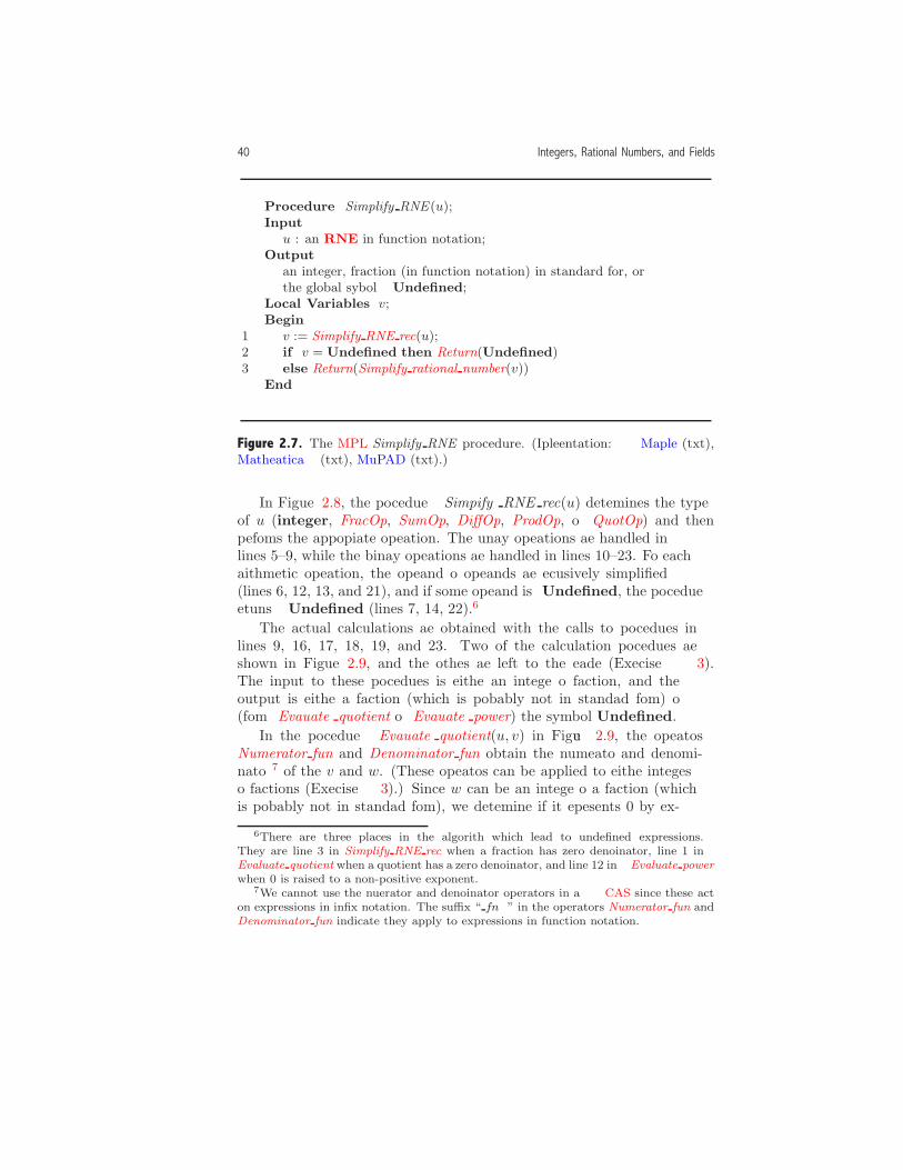
40 Integers, Rational Numbers, and Fields
Procedure Simplify RNE (u);Input
u : an RNE in function notation;Output
an integer, fraction (in function notation) in standard form, orthe global symbol Undefined;
Local Variables v;Begin
1 v := Simplify RNE rec(u);2 if v = Undefined then Return(Undefined)3 else Return(Simplify rational number(v))
End
Figure 2.7. The MPL Simplify RNE procedure. (Implementation: Maple (txt),Mathematica (txt), MuPAD (txt).)
In Figure 2.8, the procedure Simplify RNE rec(u) determines the typeof u (integer, FracOp, SumOp, DiffOp, ProdOp, or QuotOp) and thenperforms the appropriate operation. The unary operations are handled inlines 5–9, while the binary operations are handled in lines 10–23. For eacharithmetic operation, the operand or operands are recursively simplified(lines 6, 12, 13, and 21), and if some operand is Undefined, the procedurereturns Undefined (lines 7, 14, 22).6
The actual calculations are obtained with the calls to procedures inlines 9, 16, 17, 18, 19, and 23. Two of the calculation procedures areshown in Figure 2.9, and the others are left to the reader (Exercise 3).The input to these procedures is either an integer or fraction, and theoutput is either a fraction (which is probably not in standard form) or(from Evaluate quotient or Evaluate power) the symbol Undefined.
In the procedure Evaluate quotient(u, v) in Figure 2.9, the operatorsNumerator fun and Denominator fun obtain the numerator and denomi-nator7 of the v and w. (These operators can be applied to either integersor fractions (Exercise 3).) Since w can be an integer or a fraction (whichis probably not in standard form), we determine if it represents 0 by ex-
6There are three places in the algorithm which lead to undefined expressions.They are line 3 in Simplify RNE rec when a fraction has zero denominator, line 1 inEvaluate quotient when a quotient has a zero denominator, and line 12 in Evaluate powerwhen 0 is raised to a non-positive exponent.
7We cannot use the numerator and denominator operators in a CAS since these acton expressions in infix notation. The suffix “ fun” in the operators Numerator fun andDenominator fun indicate they apply to expressions in function notation.

2.2. Rational Number Arithmetic 41
Procedure Simplify RNE rec(u);Input
u : an RNE in function notation;Output
an integer, fraction (in function notation), or the global symbolUndefined;
Local Variables v, w;Begin
1 if Kind(u) = integer then Return(u)2 elseif Kind(u) = FracOp then3 if Denominator fun(u) = 0 then Return(Undefined)4 else Return(u)5 elseif Number of operands(u) = 1 then6 v := Simplify RNE rec(Operand(u, 1));7 if v = Undefined then Return(Undefined);8 elseif Kind(u) = SumOp then Return(v)9 elseif Kind(u) = DiffOp then Return(Evaluate product(−1, v))10 elseif Number of operands(u) = 2 then11 if Kind(u) ∈ {SumOp,ProdOp,DiffOp,QuotOp} then12 v := Simplify RNE rec(Operand(u, 1));13 w := Simplify RNE rec(Operand(u, 2));14 if v = Undefined or w = Undefined then
Return(Undefined)15 else16 if Kind(u) = SumOp then
Return(Evaluate sum(v, w))17 elseif Kind(u) = DiffOp then
Return(Evaluate difference(v, w))18 elseif Kind(u) = ProdOp then
Return(Evaluate product(v, w))19 elseif Kind(u) = QuotOp then
Return(Evaluate quotient(v, w))20 elseif Kind(u) = PowOp then21 v := Simplify RNE rec(Operand(u, 1));22 if v = Undefined then Return(Undefined)23 else Return(Evaluate power(v,Operand(u, 2)))
End
Figure 2.8. The MPL Simplify RNE rec procedure. (Implementation: Maple(txt), Mathematica (txt), MuPAD (txt).)

42 Integers, Rational Numbers, and Fields
Procedure Evaluate quotient(v, w);Input v, w : an integer or a fraction in function notation with
non-zero denominator;Output
a fraction in function notation or the global symbol Undefined;Begin
1 if Numerator fun(w) = 0 then Return(Undefined)2 else Return(FracOp(Numerator fun(v) ∗Denominator fun(w),
Numerator fun(w) ∗Denominator fun(v)))End
Procedure Evaluate power(v, n);Input
v : an integer or a fraction in function notation withnon-zero denominator;
n : an integer;Output
a fraction in function notation or the global symbol Undefined;Local Variables s;Begin
1 if Numerator fun(v) �= 0 then2 if n > 0 then3 s := Evaluate power(v, n− 1);4 Return(Evaluate product(s, v))5 elseif n = 0 then Return(1)6 elseif n = −1 then Return(FracOp(Evaluate quotient(v),
Numerator fun(v)))7 elseif n < −1 then8 s := FracOp(Evaluate quotient(v),Numerator fun(v));9 Return(Evaluate power(s,−n))10 elseif Numerator fun(v) = 0 then11 if n ≥ 1 then Return(0)12 elseif n ≤ 0 then Return(Undefined)
End
Figure 2.9. The MPL Evaluate quotient and Evaluate power procedures. (Im-plementation: Maple (txt), Mathematica (txt), MuPAD (txt).)
amining Numerator fun(w) (line 1). The procedure Evaluate power(v, n),which evaluates v to the exponent n, obtains the result by recursion on thepower (lines 3 and 9).
When these procedures and the procedure Simplify rational number areimplemented in a CAS, the only arithmetic operations used are the prim-
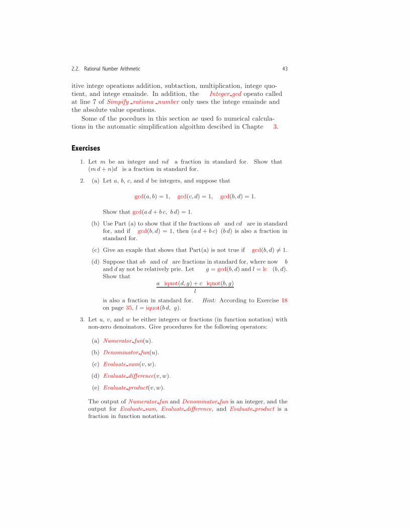
2.2. Rational Number Arithmetic 43
itive integer operations addition, subtraction, multiplication, integer quo-tient, and integer remainder. In addition, the Integer gcd operator calledat line 7 of Simplify rational number only uses the integer remainder andthe absolute value operations.
Some of the procedures in this section are used for numerical calcula-tions in the automatic simplification algorithm described in Chapter 3.
Exercises
1. Let m be an integer and n/d a fraction in standard form. Show that(md + n)/d is a fraction in standard form.
2. (a) Let a, b, c, and d be integers, and suppose that
gcd(a, b) = 1, gcd(c, d) = 1, gcd(b, d) = 1.
Show that gcd(a d + b c, b d) = 1.
(b) Use Part (a) to show that if the fractions a/b and c/d are in standardform, and if gcd(b, d) = 1, then (a d + b c)/(b d) is also a fraction instandard form.
(c) Give an example that shows that Part(a) is not true if gcd(b, d) �= 1.
(d) Suppose that a/b and c/d are fractions in standard form, where now band d may not be relatively prime. Let g = gcd(b, d) and l = lcm(b, d).Show that
a · iquot(d, g) + c · iquot(b, g)
l
is also a fraction in standard form. Hint: According to Exercise 18on page 35, l = iquot(b d, g).
3. Let u, v, and w be either integers or fractions (in function notation) withnon-zero denominators. Give procedures for the following operators:
(a) Numerator fun(u).
(b) Denominator fun(u).
(c) Evaluate sum(v, w).
(d) Evaluate difference(v, w).
(e) Evaluate product(v, w).
The output of Numerator fun and Denominator fun is an integer, and theoutput for Evaluate sum, Evaluate difference, and Evaluate product is afraction in function notation.
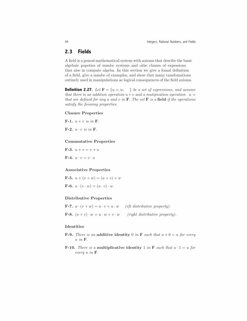
44 Integers, Rational Numbers, and Fields
2.3 Fields
A field is a general mathematical system with axioms that describe the basicalgebraic properties of number systems and other classes of expressionsthat arise in computer algebra. In this section we give a formal definitionof a field, give a number of examples, and show that many transformationsroutinely used in manipulations are logical consequences of the field axioms.
Definition 2.27. Let F = {u, v, w, . . .} be a set of expressions, and assumethat there is an addition operation u+v and a multiplication operation u ·vthat are defined for any u and v in F. The set F is a field if the operationssatisfy the following properties.
Closure Properties
F-1. u+ v is in F.
F-2. u · v is in F.
Commutative Properties
F-3. u+ v = v + u.
F-4. u · v = v · u.
Associative Properties
F-5. u+ (v + w) = (u+ v) + w.
F-6. u · (v · w) = (u · v) · w.
Distributive Properties
F-7. u · (v + w) = u · v + u · w (left distributive property).
F-8. (u+ v) · w = u · w + v · w (right distributive property).
Identities
F-9. There is an additive identity 0 in F such that u+ 0 = u for everyu in F.
F-10. There is a multiplicative identity 1 in F such that u · 1 = u forevery u in F.

2.3. Fields 45
Inverses
F-11. Each element u in F has an additive inverse in F denoted by (−u)such that u+ (−u) = 0.
F-12. Each element u �= 0 in F has a multiplicative inverse in F de-noted by u−1 such that u · u−1 = 1.
Although the field axioms are expressed in terms of a familiar nota-tion that suggests the nature of the operations, we caution the reader notto assume more about the notation than is formally stated in the defi-nition. For example, although + is an addition-like operation and · is amultiplication-like operation, the operations can be quite different fromwhat we ordinarily associate with addition and multiplication.8 In a sim-ilar way, the notation for identities and inverses are only names for theseexpressions. For example, although the multiplicative inverse is expressedusing the power notation u−1, at this point it doesn’t imply anything abouta power operation.9
Example 2.28. A simple example of a field is the set Q of rational numbers,where the two field operations are ordinary addition and multiplication.In this case, the additive identity is the integer 0 and the multiplicativeidentity the integer 1. The additive inverse of a rational number u is −u,and the multiplicative inverse of u = a/b �= 0 is 1/u = b/a. In a similarway, the set R of (mathematical) real numbers is a field. �
Example 2.29. Consider the set of real numbers of the form a+b√2, where
a and b are rational numbers. Let’s show that this set with the operationsof ordinary addition and multiplication of real numbers is a field. Sincethis set is included in R, we only verify the properties F-1, F-2, F-11, andF-12, and assume that the others are inherited from the properties of thereal numbers. Since,
(a+ b√2) + (c+ d
√2) = (a+ c) + (b+ d)
√2,
(a+ b√2) · (c+ d
√2) = (a c+ 2 b d) + (b c+ a d)
√2,
the sum and product have the proper form, and so F-1 and F-2 are satisfied.The additive inverse of a+b
√2 is (−a)+(−b)√2. To find the multiplicative
inverse ofa+ b
√2 �= 0, (2.55)
8For example, in Exercise 3 we describe a field with four expressions where u+u = 0for all expressions in the field.
9For example, in the field Z5 (see page 52), there is an expression u �= 1 such thatu = u−1.

46 Integers, Rational Numbers, and Fields
we must find rational numbers x and y such that
(a+ b√2) · (x + y
√2) = 1.
Expanding the left side of the equality, we obtain
(a x+ 2 b y) + (b x+ a y)√2 = 1.
In this equation, b x + a y = 0 because, if this were not so, we could solvefor√2 and conclude that it is a rational number. Therefore, we have two
equations
b x+ a y = 0, a x+ 2 b y = 1,
and solving for x and y, we obtain
(a+ b√2)−1 = x+ y
√2 =
a
a2 − 2 b2+
−ba2 − 2 b2
√2.
The multiplicative inverse can also be found by rationalizing the denomi-nator:
1a+ b
√2=
1a+ b
√2
a− b√2
a− b√2=
a
a2 − 2b2+
−ba2 − 2b2
√2.
By the way, the denominator that appears in the expression on the rightsatisfies
a2 − 2b2 �= 0. (2.56)
To see why, first, if b = 0, then from the condition (2.55) we must havea �= 0, and the condition (2.56) follows. Next, if b �= 0, then if a2−2 b2 = 0,we have
√2 =
√a2/b2 = |a/b| which implies that
√2 is a rational number.
Since√2 is irrational, the condition (2.56) must be true.
The field described in this example is denoted by Q(√2). The notation
indicates that the field is constructed by adjoining the expression√2 to
the base field Q. �
Example 2.30. Consider the set of expressions of the form a + b ı whereı =√−1 and a and b are rational numbers. This set is a field with the two
operations + and · defined by
(a+ b ı) + (c+ d ı) = (a+ c) + (b + d) ı, (2.57)
(a+ b ı) · (c+ d ı) = (a c− b d) + (c b+ a d) ı. (2.58)
(The addition and multiplication operations that are inside the parenthe-ses on the right sides of the equations are addition and multiplication of

2.3. Fields 47
rational numbers.) The additive inverse of a+ b i is (−a) + (−b) ı, and, fora+ b ı �= 0, the multiplicative inverse is
(a+ b ı)−1 =a
a2 + b2+
(−b)a2 + b2
ı
This field, which is denoted by Q(ı), is known as the Gaussian rationalnumber field.
In a similar way, the set C of complex numbers a+b ı, where a and b arereal numbers, is a field with the operations + and · defined by Equations(2.57) and (2.58). �
Example 2.31. Consider the set of expressions of the form
u = a+ b√2 + c
√3 + d
√2√3,
where a, b, c, and d are rational numbers together with the operations ofordinary addition and multiplication. We leave to the reader the verifica-tion that the sum and product of two of these expressions are also in thisform and the derivation of expressions for the additive and multiplicativeinverses (Exercise 2(a)). This field is denoted by Q(
√2,√3) where the
notation indicates that the field is constructed from the base field Q byadjoining the two radicals
√2 and
√3. By grouping terms, we have
a+ b√2 + c
√3 + d
√2√3 = (a+ b
√2) + (c+ d
√2)√3,
which shows that we can also view this field as (Q(√2))(√3), where the
notation indicates that the field is constructed by first adjoining√2 to Q
to obtain Q(√2) and then adjoining
√3 to Q(
√2). �
Example 2.32. Consider the set of rational expressions of the form
u(x)v(x)
where u(x) and v(x) �= 0 are polynomials in x with rational number co-efficients. We interpret this definition in a broad sense to include simplerexpressions such as polynomials, fractions, and integers. This set, togetherwith the addition and multiplication operations defined by
u(x)v(x)
+r(x)s(x)
=Algebraic expand (u(x) s(x) + v(x) r(x))
Algebraic expand(v(x) s(x))
and

48 Integers, Rational Numbers, and Fields
u(x)v(x)
· r(x)s(x)
=Algebraic expand(u(x) r(x))Algebraic expand(v(x) s(x))
,
is a field. In this case, the identities are the integers 0 and 1, the additiveinverse of u(x)/v(x) is the rational expression ((−1) · u(x))/v(x) (with thenumerator expanded), and if u(x)/v(x) �= 0, the multiplicative inverse isv(x)/u(x). The field of rational expressions is denoted by Q(x), where thenotation indicates the field is obtained by adjoining the symbol x to thebase field Q.
Although the fields Q(x) and Q(ı) use a similar notation to denote thefield, the expressions in Q(x) are more complicated than those in Q(ı).In the latter case, the symbol ı satisfies the simplification transformationı2 = −1, and so involved rational expressions in the symbol ı simplify tothe appropriate form. For example,
2 + 3 ı4 + 5 ı+ 6 ı2
= 11/29 + (−16/29) ı.
On the other hand, since the symbol x does not satisfy a simplificationtransformation,
2 + 3 x4 + 5 x+ 6 x2
does not simplify. �
Example 2.33. Not all of the familiar sets of numbers are fields. Forexample, the set Z of integers is not a field because it does not containmultiplicative inverses. However, Z does satisfy all of the field properties,except F-12. In addition, the integers satisfy the property:
if a · b = 0, then either a = 0 or b = 0.
This property is described by saying that Z has no zero divisors. A math-ematical system that satisfies field axioms F-1 through F-11 and has nozero divisors is called an integral domain. �
Consequences of the Field Axioms
The field axioms embody the basic transformation rules that are needed toperform calculations with expressions in F. Other properties and transfor-mation rules that are used routinely in calculations are derived as logicalconsequences of the basic axioms. This process is illustrated in the proofsof the next two theorems.

2.3. Fields 49
Theorem 2.34. Let F be a field.
1. The identities 0 and 1 in F are unique.
2. Every u in F has a unique additive inverse (−u), and if u �= 0, it hasa unique multiplicative inverse u−1.
Proof: Notice that the field axioms do not say that identities and inversesare unique, only that they exist. Could there be a field that has, forexample, two distinct additive identities? Of course, the answer is no, butthis must be verified from the axioms.
To prove (1), suppose that there were two additive identities, say 0 and0′. Then, by F-9, with 0′ acting as an additive identity,
0 = 0 + 0′.
Applying F-3 to the right side of the equality, we have
0 = 0′ + 0.
Applying F-9 with 0 acting as an additive identity, we obtain
0 = 0′.
In a similar way, we can show that the multiplicative identity is unique.Statement (2) follows in a similar manner (Exercise 4). �
Theorem 2.35. Let u and v be expressions in a field F. Then,
1. u · 0 = 0;
2. (−u) = (−1) · u;
3. (−0) = 0;
4. 1−1 = 1;
5. (−1)−1 = −1;6. (−u) · (−v) = u · v;
7. If u �= 0, then (u−1)−1 = u;
8. If u �= 0 and v �= 0, then (u · v)−1 = u−1 · v−1.
50 Integers, Rational Numbers, and Fields
Proof: To prove (1), by F-9,
u · (u+ 0) = u · u,
and so by F-7,u · u+ u · 0 = u · u.
Adding the additive inverse of u ·u to both sides of this equality and usingF-9, we have
(u · u+ u · 0) + (−(u · u)) = u · u+ (−(u · u)) = 0. (2.59)
Next, using the field axioms, the left side of this equation can be trans-formed in the following way:
(u · u+ u · 0) + (−(u · u)) = (−(u · u)) + (u · u+ u · 0) (by F-3)= ((−(u · u)) + u · u) + u · 0 (by F-5)= (u · u+ (−(u · u))) + u · 0 (by F-3)= 0 + u · 0 (by F-11)= u · 0 + 0 (by F-3)= u · 0 (by F-9). (2.60)
Therefore, by comparing Equations (2.59) and (2.60), we have u · 0 = 0.To prove (2), we show first that (−1) ·u is the additive inverse of u. We
have
u+ (−1) · u = u · 1 + u · (−1) (by F-4 and F-10)= u · (1 + (−1)) (by F-7)= u · 0 (by F-11)= 0 (by Part (1) of the theorem).
Therefore, by statement (2) of Theorem 2.34, (−u) = (−1) · u.The proofs of the remaining statements of the theorem are left to the
reader (Exercise 5). �
Theorem 2.36. Suppose that u and v are in a field F with u · v = 0. Then,either u = 0 or v = 0.
This property is described by saying that a field has no zero divisors.The proof of the theorem is left to the reader (Exercise 6).
2.3. Fields 51
Subtraction, Division and Exponentiation in a Field
Although subtraction, division, and exponentiation are not directly part ofthe field definition, the operations are easily defined using the field opera-tions.
Definition 2.37. Let u and v be expressions in a field F. The subtraction(or difference) operation is defined by
u− v = u+ (−v), (2.61)
where (−v) is the additive inverse of v.
Using Theorem 2.35(2), subtraction can also be represented as
u− v = u+ (−1) · v,
which is the automatically simplified form for differences in most computeralgebra systems.
Definition 2.38. Let u and v �= 0 be expressions in a field F. The divisionor quotient operation is defined by
u/v = u · v−1. (2.62)
The automatic simplification process in most computer algebra systemstransforms a quotient to the form on the right in Equation (2.62).
Definition 2.39. Let u be an expression in a field F, and let n be an integer.The exponentiation or power operation un is defined with the recursivedefinition.
1. If u �= 0 and n = −1, then u−1 is the multiplicative inverse of u.
2. If u �= 0 and n �= −1, then
un =
un−1 · u, when n ≥ 1,1, when n = 0,(u−1
)(−n), when n ≤ −2.
3. If u = 0, then
0n ={0 when n ≥ 1,Undefined, when n ≤ 0.

52 Integers, Rational Numbers, and Fields
For example, a strict interpretation of the definition gives (for u �= 0)
u−3 = (u−1)3 = (u−1)2 · u−1 = ((u−1)1 · u−1) · u−1
= (((u−1)0 · u−1) · u−1) · u−1 = ((1 · u−1) · u−1) · u−1
= (u−1 · u−1) · u−1.
The exponentiation operation satisfies the following properties.
Theorem 2.40. Let u �= 0 and v �= 0 be expressions in a field F, and let mand n be integers. Then,
1. (u · v)m = um · vm;
2. um · un = um+n;
3. (um)n = umn.
When either u = 0 or v = 0, the properties hold as long as the expressionson both sides of the equal sign are defined.
Proof: To prove Part (1), first assume that u �= 0 and v �= 0. The proof form ≥ 0 uses mathematical induction. The base case m = 0 follows directlyfrom Definition 2.39(2). For m ≥ 1, assume that the relation is true form − 1. Then, using Definition 2.39(2) and the induction hypothesis, wehave
(u · v)m = (u · v)m−1 · (u · v) = um−1 · vm−1 · u · v = um · vm.For m = −1, the relation follows from Theorem 2.35(8). For m ≤
−2, we have −m ≥ 2 and so using the above case together with Defini-tion 2.39(2) and Theorem 2.35(8), we have
(u · v)m = ((u · v)−1)−m = (u−1 · v−1)−m = (u−1)−m · (v−1)−m = um · vm.For the case when either u = 0 or v = 0, the relation is defined when
m ≥ 1 and follows from Definition 2.39(3).The proofs for Parts (2) and (3) are left to the reader (Exercise 9). �
Finite Fields
Some fields contain only a finite number of expressions. For example, letp > 1 be an integer, and consider the set Zp = {0, 1, . . . , p− 1}. Define anaddition operation ⊕p and multiplication operation ⊗p by
a⊕pb = irem(a+ b, p), a⊗pb = irem(a · b , p)where + and · are the ordinary integer operations. For example, whenp = 5, the operations are given in the following operation tables.

2.3. Fields 53
⊕5 0 1 2 3 40 0 1 2 3 41 1 2 3 4 02 2 3 4 0 13 3 4 0 1 24 4 0 1 2 3
⊗5 0 1 2 3 40 0 0 0 0 01 0 1 2 3 42 0 2 4 1 33 0 3 1 4 24 0 4 3 2 1
It is apparent from the tables that each element has an additive inverse,and each non-zero element has a multiplicative inverse. Since Z5 inheritsthe field properties F-3 through F-10 from the integers, it is a field.
However, Z6 is not a field. In this case, the ⊗6 table is given in thefollowing table.
⊗6 0 1 2 3 4 50 0 0 0 0 0 01 0 1 2 3 4 52 0 2 4 0 2 43 0 3 0 3 0 34 0 4 2 0 4 25 0 5 4 3 2 1
It is apparent that 2, 3, and 4 do not have multiplicative inverses.The next theorem describes when Zp is a field.
Theorem 2.41. Let p > 1 be an integer. The set Zp with the operations ⊕pand ⊗p is a field if and only if p is a prime number.
Proof: Let’s assume that p is prime and show that Zp is a field. Sincethe closure properties F-1 and F-2 follow from the definitions of ⊕p and⊗p, and the properties F-3 through F-10 are inherited from the integers,we only need to verify the inverse properties. Let s be in Zp. The additiveinverse of s is given by p− s.
We verify the multiplicative inverse property by giving an algorithmthat obtains the inverse. Let 0 < s ≤ p − 1. Since p is prime, using theextended Euclidean algorithm, we obtain integers m and n such that
m · s+ n · p = 1. (2.63)
When m is in the range 0 < m ≤ p − 1, we can show that s−1 = m.Unfortunately, m may lie outside of this range although m cannot be amultiple of p. (If m were a multiple of p, then by Equation (2.63), p|1which is not true.) Therefore, to obtain the inverse, divide m by p to get
m = q · p+ r, (2.64)

54 Integers, Rational Numbers, and Fields
with 1 ≤ r < p. Using Equations (2.63) and (2.64), we obtain
s⊗pr = irem(s · r, p)= irem(s · (m− q · p), p)= irem((1− p · n)− s · q · p, p)= irem(1− p · (n+ s · q), p)= 1,
which implies that r = s−1. It is now a simple matter to give a procedurethat finds s−1 (Exercise 11).
We have shown that whenever p is prime, Zp is a field. The proof ofthe converse statement is left to the reader (Exercise 12). �
Example 2.42. Let p = 47 and s = 16. The extended Euclidean algorithmgives m = 3, n = −1, and since m is in Z47, 16−1 = 3.
Next let p = 47 and s = 17. In this case, m = −11 and n = 4, and sincem is not in Z47, we obtain the inverse with 17−1 = irem(−11, 47) = 36. �
The next theorem gives three simple arithmetic relationships in Zp.
Theorem 2.43. Let p be a prime, and let u and v be in Zp. Then,
1. u⊕p · · · ⊕pu︸ ︷︷ ︸p
= 0, where the notation indicates the sum has p copies
of u;
2. (u⊕pv)p = up⊕pvp;3. up = u.
The relationship (3) is known as Fermat’s little theorem.
Proof: Part (1) follows from
u⊕p · · · ⊕pu︸ ︷︷ ︸p
= irem(u+ · · ·+ u︸ ︷︷ ︸p
, p) = irem(p · u, p) = 0.
To show Part (2), we have, using the binomial theorem,
(u⊕pv)p =p∑j=0
(p!
(p− j)! j!
)(up−j⊗pvj
)
= up ⊕
p−1∑j=1
(up−j⊗pvj
)⊕p · · · ⊕p (up−j⊗pvj)︸ ︷︷ ︸p!
(p−j)! j!
⊕ vp. (2.65)

2.3. Fields 55
However, since p divides the integerp!
(p− j)! j!, for 1 ≤ j ≤ p− 1, we have
by Part (1) of the theorem(up−j⊗pvj
)⊕p · · · ⊕p (up−j⊗pvj)︸ ︷︷ ︸p!
(p−j)! j!
= 0
which eliminates the sum in parentheses in Equation (2.65). Therefore,(u⊕pv)p = up⊕pvp.
Part (3) is proved using mathematical induction on u. First, the rela-tionship is true when u = 0 or u = 1. Suppose now that 2 ≤ u ≤ p − 1,and assume that the relationship holds for u − 1. Using Part (2) and theinduction hypothesis, we have
up = ((u − 1)⊕p1)p = (u − 1)p⊕p1p = (u − 1)⊕p1 = u.
Part (3) of the theorem has a number of useful consequences. First, itshows that Part (2) of the theorem is a simple relationship because bothsides simplify to u⊕pv. Another application has to do with the computationof multiplicative inverses in Zp. For u �= 0, (3) implies that up−2⊗pu = 1,and therefore u−1 = up−2. �
Other examples of finite fields are given in Exercise 3 and Exercise 7,page 164. Finite fields are used in some modern greatest common divisorand factorization algorithms for polynomials (see Chapter 9).
Algebraic Numbers
Definition 2.44. A complex number c is called an algebraic number if itis the root of a polynomial equation u(x) = 0, where u(x) is in Q[x] withpositive degree.10 The set of algebraic numbers is denoted by A.
Example 2.45. The following are algebraic numbers because each one sat-isfies the polynomial equation on the right:
x = 2/3, 3 x− 2 = 0,
x =√2, x2 − 2 = 0,
x = i =√−1, x2 + 1 = 0,
x = 71/3, x3 − 7 = 0,10Although the terms algebraic number defined here and algebraic expression defined
in Chapter 1 are similar, the mathematical concepts are quite different.

56 Integers, Rational Numbers, and Fields
x =1+√5
2, x2 − x+ 1 = 0, (2.66)
x =√2 +√2, x4 − 4 x2 + 2 = 0,
x =√2 +√3, x4 − 10 x2 + 1 = 0. �
Definition 2.46. An expression u is an explicit algebraic number if itsatisfies one of the following rules:
EAN-1. u is an integer or fraction.
EAN-2. u = vw, with v �= 0 an explicit algebraic number and w an integeror fraction.
EAN-3. u is a product or sum of explicit algebraic numbers.
All of the expressions in Example 2.45 are explicit algebraic numbers.However, not all algebraic numbers are explicit. This is a consequence ofGalois theory11 which states that it is impossible to express the roots of allpolynomial equations with degree ≥ 5 as explicit algebraic numbers. Forexample the polynomial equation
u = 4 x5 − 10 x2 + 5 = 0 (2.67)
has three distinct real roots and two distinct (non-real) complex roots, butnone of them are explicit. In other words, some algebraic numbers can beexpressed explicitly while others are only known implicitly as the root ofan equation.
Definition 2.47. An algebraic number that is not explicit is called an im-plicit algebraic number.
The five roots of Equation (2.67) are implicit algebraic numbers.Given an explicit algebraic number, it is often possible to find with
some simple manipulations a polynomial that has the number as a root.For example, to find the polynomial associated with
x =√2 +√3, (2.68)
first square both sides, and then move the integer part to the left side
x2 − 5 = 2√2√3.
11The theory is named after the brilliant French mathematician Evariste Galois (1811-1832) who outlined its essential ideas. Galois was killed in a duel at the age of 20.
2.3. Fields 57
Squaring both sides again, we get
x4 − 10 x2 + 1 = 0. (2.69)
For a more complicated explicit algebraic number, the manipulations tofind the polynomial are more involved. In Section 7.2 we give an algorithmthat finds a polynomial that has a given explicit algebraic number as a root.
Now, let’s reverse the process to find the roots of Equation (2.69). First,solving for x2,
x2 = 5± 2√2√3. (2.70)
Next, solving Equation (2.70) for x, we get the four roots
x = ±√5± 2
√2√3. (2.71)
Notice that the explicit form (2.71) is quite different from the form (2.68).Since Equation (2.71) gives all four roots of Equation (2.69), we have
±√2±√3 = ±
√5± 2
√2√3. (2.72)
It is easy to check this relationship by squaring both sides of the equation.However, this relationship points out a difficulty that arises with explicitalgebraic numbers: namely, they may have more than one representation.This is not particularly surprising because by simply rationalizing a de-nominator, two representations can look different. For example,
(2 + 3√2)−1 = −1/7 + 3/14
√2.
In general, however, it is a difficult simplification problem to determinewhen two explicit algebraic expressions are the same number.12 For exam-ple,
√2 +√3 +√5 =
√2√5 · 101/4 + 103/4 +
√3√7√10 + 20
101/8. (2.73)
Algebraic Number Fields
Definition 2.48. An algebraic number field F is a field constructed fromthe base field Q by adjoining a finite number of algebraic numbers.
Example 2.49. Q(√2),Q(i), andQ(
√2,√3) are algebraic number fields. �
12See Davenport, Siret, and Tournier [29] for a discussion of this problem.

58 Integers, Rational Numbers, and Fields
We give algorithms for computations in some simple algebraic numberfields in Section 4.3.
The set A of all (implicit or explicit) algebraic numbers is also a field13
but not an algebraic number field in the sense of Definition 2.48 becauseit cannot be constructed from Q by adjoining a finite number of algebraicnumbers.
Transcendental Numbers
Definition 2.50. A complex number c that is not an algebraic number iscalled a transcendental number.
The numbers π and e are real numbers that are transcendental.14 Inaddition, although the number eπ is also transcendental, it is not knownwhether π + e, π · e, or πe are algebraic or transcendental.
Explicit Algebraic Numbers: Theory versus Practice
In Exercise 15, we describe an operator Explicit algebraic number(u) thatreturns true when u is an explicit algebraic number and otherwise returnsfalse. Since we assume that the simplification context for the operator isautomatic simplification, there are algebraic expressions that the operatordetermines are explicit algebraic numbers even though the expressions areundefined in a mathematical sense. For example, the expression
u =1
21/2 + 31/2 − (5 + 2 · 21/2 · 31/2
)1/2is undefined mathematically because the denominator simplifies to 0 (seeEquation (2.72)), but this is not obtained by automatic simplification inMaple, Mathematica or MuPAD. For this reason, implementations of theoperator in these systems obtain Explicit algebraic number(u)→ true. Infact, it is a difficult problem to determine when an explicit algebraic numbersimplifies to 0. We return to this point in Section 7.2.
Exercises
1. Consider the set of real numbers that have the form a+b 21/3 +c 22/3 wherea, b, and c are rational numbers. Show that this set with the operations ofordinary addition and multiplication is a field.
13This is proved in Theorem 7.16 on page 289.14For proofs of the transcendence of π and e, see Hardy and Wright [43].

2.3. Fields 59
2. (a) Verify that Q(√
2,√
3) described in Example 2.31 is a field.
(b) Let u be in Q(√
2,√
3). Give a procedure Mult inv 23 (u) that findsthe multiplicative inverse in this field.
3. Let x and y be symbols, and consider the set of expressions F = {0, 1, x, y}with the operations defined by
⊕ 0 1 x y
0 0 1 x y
1 1 0 y x
x x y 0 1
y y x 1 0
⊗ 0 1 x y
0 0 0 0 0
1 0 1 x y
x 0 x y 1
y 0 y 1 x
Show that F is a field.
4. Prove Theorem 2.34(2). Hint: For the uniqueness of the additive inverse,suppose that there are two expressions x and y such that u + x = 0 andu+ y = 0. Show that x = y. In a similar way, show that the multiplicativeinverse is unique.
5. Prove properties (3) through (8) of Theorem 2.35.
6. Prove Theorem 2.36.
7. Let u and v be expressions in a field F. Show that the division operationsatisfies the following.
(a) u/1 = u.
(b) u/(−1) = (−u).
(c) If u �= 0 and v �= 0, (u/v)−1 = v/u.
8. Let u �= 0 be an expression in a field F. Prove that the exponentiationoperation satisfies the following.
(a) u−1 n= u−n.
(b) u−1 n= (un)−1.
Do not use Theorem 2.40 in this exercise.
9. (a) Prove Theorem 2.40(2). Hint: Use mathematical induction on n ≥ 0,and consider the three cases m + n − 1 ≥ 0, m + n − 1 = 0, andm + n− 1 ≤ −1. The relations in Exercise 8 are useful here.
(b) Prove Theorem 2.40(3). Hint: The relations in Exercise 8 are usefulhere.
10. Are Theorem 2.43(1) and Theorem 2.43(2) true when p is not a prime?Either prove statements (1) and (2) in this setting or give examples thatshow that the statements are not always true.
11. Let p be prime, and let s, t �= 0 be in Zp.

60 Integers, Rational Numbers, and Fields
(a) Give a procedure Multiplicative inverse p(t, p) that obtains the mul-tiplicative inverse t−1.
(b) Give a procedure Division p(s, t , p) that obtains s/t in Zp.
12. Let p > 1 be an integer. Show that if Zp is a field, then p is prime.
13. Show that each of the following is an algebraic number by finding a (non-zero) polynomial with rational number coefficients that each one satisfies.
(a)√
7 +√
11.
(b)√
7 +√
11.
(c) 11 +
√2
.
(d) 1 +√
2√
3.
(e)√
2 +√
3 +√
5.
14. Using the fact that π is transcendental, show that each of the following isalso transcendental.
(a) π2.
(b) 1/π.
15. Give a procedure Explicit algebraic number(u) that returns true if analgebraic expression is an explicit algebraic number and false otherwise.
16. Suppose that u is an explicit algebraic number. Give a procedure
Nest depth(u)
that gives the nesting depth of u which is defined using the followingrules.
(a) If u is an integer or fraction, then Nest depth(u) → 0.
(b) If u = ar, where r is a fraction, then
Nest depth(u) → 1 + Nest depth(a).
(c) If u is a sum or a product with n operands then
Nest depth(u) → Max ({Nest depth(Operand(u, 1)),
. . . ,Nest depth(Operand(u, n))}) .
For example,
Nest depth 5 · 1 + 21/21/3
→ 2.

2.3. Fields 61
17. Let u be an algebraic expression. Give a procedure Variables 2 (u) thatreturns the set of generalized variables of u that are not explicit algebraicnumbers. For example,
Variables 2 (21/2 x + 3 · 52/3 y + z) → {x, y, z}.
Note: The Variables operator described on page 12 is one of our primitivepolynomial operators.
18. Give a procedure Alg collect(u) that collects explicit algebraic number co-efficients of like terms in a sum u. If u is not a sum, then return u. Forexample,
Alg collect√
2x y + 3x y +√
3 x + 4x →√
2 + 3 x y +√
3 + 4 x,
Alg collect√
2√
3 +√
2 z +√
3 z →√
2√
3 +√
2 +√
3 z,
Alg collect√
2x y + 2x y + x →√
2 + 2 x y + x,
Alg collect a√
2x + x → a√
2x + x .
In the last example, collection is not done because the input expression isnot a sum.
19. A Gaussian rational number c is in standard form if it has one of thefollowing forms:
(a) c is a rational number in standard form.
(b) c = ı.
(c) c = b · ı, where b �= 0, 1 is a rational number in standard form.
(d) c = a+b·ı, where a �= 0 and b �= 0, 1 are rational numbers in standardform.
(e) c = a + ı, where a �= 0 is a rational number in standard form.
In forms (c), (d), and (e) the order of the operands in a sum or product isa significant property of the standard form. (For example, the expressionı ·b is out of order, and so is not in standard form.) In this exercise, we askyou to give an algorithm Simplify Gaussian(u) that transforms a Gaussianrational number expression (defined below) to either a Gaussian rationalnumber in standard form or the symbol Undefined when a division byzero is encountered. The Gaussian rational number expressions (GRNE)are the ones that satisfy one of the following rules:
GRNE-1. u is an integer.
GRNE-2. u is a fraction. At this point, we allow for the possibility ofa fraction with zero denominator. The algorithm will recognize thatsuch an expression is undefined.

62 Integers, Rational Numbers, and Fields
GRNE-3. u is the symbol ı.
GRNE-4. u is a unary or binary sum with operands that are GRNEs.
GRNE-5. u is a unary difference or a binary difference with operandsthat are GRNEs.
GRNE-6. u is a binary product with operands that are GRNEs.
GRNE-7. u is a quotient with operands that are GRNEs.
GRNE-8. u is a power with a base that is a GRNE and an exponent thatis an integer.
To bypass the automatic simplification rules in a CAS, represent the arith-metic operations and fractions with the function forms given in Figure 2.6on page 39. For example,
Simplify Gaussian(SumOp(
FracOp(1, 2),QuotOp(1,SumOp(3, ı))))
→ SumOp(FracOp(4, 5),ProdOp(FracOp(−1, 10), ı)).
Further Reading
2.1 The Integers. See Birkhoff and Mac Lane [10], Dean [31], or Pinter [79]for derivations of properties of the integers. Euclid’s algorithm appears in BookSeven of Euclid’s Elements, Propositions 1 and 2. See Calinger [19], pages 119-120 for Euclid’s original approach. An explicit formula for the gcd is given inPolezzi [80]. See Cormen, Leiserson and Rivest [28] and von zur Gathen andGerhard [96] for algorithms for the prime factorization of positive integers. Lib-brecht [61] has an historical essay on the Chinese remainder theorem. Davis andHersh [30] has an interesting discussion of the Chinese remainder theorem andits generalizations.
2.3 Fields. See Birkhoff and Mac Lane [10], Dean [31], or Pinter [79] for a
discussion of fields and algebraic numbers. A history of the field concept is given
in Kleiner [52], [53]. The theory and application of finite fields is described in
Lidl and Niederreiter [62]. See Jeffrey and Rich [49] for a discussion of some
simplification problems with square roots. An interesting discussion of algebraic
and transcendental numbers is given in Stevenson [93].

3
Automatic Simplification
The automatic simplification process is defined as a collection of algebraicand trigonometric simplification transformations that is applied to an ex-pression as part of the evaluation process. In this chapter we take anin-depth look at the algebraic component of this process.
In Section 3.1 we describe the automatic simplification process in aninformal way, focusing on which transformations should be included in theprocess and which ones are best handled by other operators. Next, wegive a precise definition of an automatically simplified algebraic expressionwhich includes an order relation that describes actions of the additive andmultiplicative commutative transformations.
In Section 3.2 we describe the basic automatic simplification algorithm.Although the algorithm is based only on the rules of elementary algebra, itis quite involved. To handle a large variety of expressions, the automaticsimplification process includes over 30 rules (or rule groups), some of whichare recursive. The problem addressed in this section is how to organize thisinvolved process into a coherent algorithm.
3.1 The Goal of Automatic Simplification
The transformation rules in automatic simplification are motivated by thefield axioms (which are assumed to hold for expressions as well as for num-ber fields) and by the transformations that are logical consequences of theseaxioms. We begin by examining the role of each of the axioms in the au-tomatic simplification process.
63

64 3. Automatic Simplification
The Basic Distributive Transformations
The (right) distributive property (field axiom F-8) has the form
(a+ b) · c = a · c+ b · c. (3.1)
This transformation is applied during automatic simplification in a rightto left manner to combine constant (integer or fraction) coefficients of liketerms in a sum. A typical transformation is
2 x+ y + (3/2)x = (7/2)x+ y.
There are, however, some similar manipulations that are omitted fromautomatic simplification. One natural generalization of this manipulationinvolves the collection of non-constant coefficients of like terms as well asthe constant ones as is done in
3 x+ a x+ y = (3 + a)x+ y. (3.2)
There are two reasons why this transformation is omitted from automaticsimplification. First, there is uncertainty about which parts of an expres-sion are the like terms and which parts are the coefficients. This happenswith the expression
a x+ b x+ b y,
for if we collect coefficients of x, we obtain (a+b)x+b y, while if we collectcoefficients of b, we obtain a x+b (x+y). In other words, since the structureof an expression by itself does not identify semantic roles such as coefficientand like term, the operation is ambiguous.
A second reason to avoid collecting non-constant coefficients has to dowith its relationship to the Algebraic expand operator. Since this operatorapplies Equation (3.1) in the opposite (left to right) direction, the collec-tion of non-constant coefficients cancels out some of its actions. For thesereasons, it is common practice in computer algebra systems to collect onlyrational number coefficients with automatic simplification. Unfortunately,this means that coefficients that are not rational numbers but play the se-mantic role of constants (e.g., π,
√2) are also not collected. For example, in
2 x+ 3 x+√2 x = 5 x+
√2 x,
we combine only the integer coefficients of x.Since automatic simplification uses the tree structure to recognize like
terms, it is only able to combine coefficients of like terms with a similarstructure. This means that the manipulation
sin(x) + 2 sin(x) = 3 sin(x)

3.1. The Goal of Automatic Simplification 65
is obtained with automatic simplification, while
1 + x+ 2 (1 + x) = 3 (1 + x) (3.3)
is not. In the latter case, the 1 + x at the far left is not a complete sub-expression of the sum and so is not structurally the same as the 1 + x inthe product 2 (1 + x).
There is another way to use distributive properties to simplify the ex-pression (3.3). If we apply the left distributive property (field axiom F-7)
a · (b+ c) = a · b+ a · cin a left to right fashion to distribute the constant 2 over 1 + x, and thenuse the distributive property again to combine coefficients of x, we obtain
1 + x+ 2 (1 + x) = 3 + 3 x. (3.4)
This manipulation is more involved because it involves the application ofthe distributive property both to distribute and collect constants. Becauseof this, there is some question about whether it belongs in automatic sim-plification or should be obtained with the Algebraic expand operator. Inaddition, if constants are distributed over sums, then what should be donewith 2 (3 + x) (4 + x)? Should the 2 be distributed over one of the twosums in the product and if so which one? This uncertainty is reflected inthe different approaches taken by computer algebra software. Maple andMuPAD achieve manipulations like Equation (3.4) with automatic simpli-fication,1 while Mathematica does not. However, all three systems achievethe manipulation
x+ 1 + (−1) (x+ 1) = 0, (3.5)
even though it also involves both the distribution and collection of con-stants.
With these considerations in mind, we include the following transfor-mation in our automatic simplification algorithm.
Definition 3.1. The basic distributive transformation in automaticsimplification refers to the collection of integer and fraction coefficients oflike terms in a sum.
Observe that the basic distributive transformation does not distributeconstants over sums2 and so does not obtain the simplifications in Equa-tions (3.4) and (3.5).
1Automatic simplification in Maple and MuPAD distributes a constant over a singlesum but does not change 2 (3 + x) (4 + x). (Implementation: Maple (mws), MuPAD(mnb).)
2A modification of the automatic simplification algorithm that does distribute con-stants over sums is described in Exercise 8, page 108.
66 3. Automatic Simplification
As a result of this transformation, a simplified sum cannot have twooperands with the same like term.3
The Basic Associative Transformations
The associative transformations are based on the additive and multiplica-tive associative field axioms (F-5 and F-6):
a+ (b + c) = (a+ b) + c, (3.6)
(a · b) · c = a · (b · c). (3.7)
The associative properties suggest that the parentheses in Equations (3.6)and (3.7) are superfluous, and so a natural way to incorporate associa-tivity into automatic simplification is simply to eliminate the parentheses.This means automatic simplification should perform the following manip-ulations:
(w + x) + (y + z) = w + x+ y + z,
((w · x) · y) · z = w · x · y · z,(((u + v) · w) · x+ y) + z = (u + v) · w · x+ y + z.
The tree structures that correspond to these simplifications are shown inFigures 3.1 and 3.2. In a structural sense, the associative transformationstend to reduce the number of levels in an expression tree by removing super-fluous addition or multiplication operators and reassigning their operandsto appropriate instances of the same operator in the tree.
When the automatic simplification process is applied to a particularsub-expression of an expression, the additive associative transformation isalways applied before the distributive transformations. The next two ex-amples show how this order of application affects the simplification process.
Example 3.2. Consider the manipulation
x+ (x+ y) = x+ x+ y = 2 x+ y.
In this case, we first apply an associative transformation that modifies thestructure of the expression and then apply a distributive transformationthat collects coefficients of like terms. On the other hand, if the distributivetransformation were applied before the associative transformation, it wouldnot combine the two unlike terms x and x + y, and so after applying theassociative transformation, the simplified form would be x+ x+ y. �
3This statement also requires that the basic associative transformation for sums beapplied before the basic distributive transformation (see Definition 3.5 and Example 3.2).

3.1. The Goal of Automatic Simplification 67
���
❅❅❅
❅❅�� ❅❅ ��
✆✆✆
���
❅❅❅
❊❊❊
+
zyxw
+
+
+w x y z
(unsimplified) (simplified)
(a) Tree structures for (w + x) + (y + z) = w + x+ y + z.
��
��
❏❏
✜✜ ❏❏
∗∗
∗∗ z
y
w x
���
✆✆✆
❊❊❊❅
❅❅w x y z
(unsimplified) (simplified)
(b) Tree structures for ((w · x) · y) · z = w · x · y · z.
Figure 3.1. Tree transformations with the basic associative transformations.
Example 3.3. Sometimes the additive associative transformation inhibitsan application of the distributive transformation. This happens with theexpression
(1 + x) + 2 (1 + x). (3.8)
(We considered a similar expression in Equation (3.3) where parentheseswere omitted from the 1 + x at the left.) In this unsimplified form, bothinstances of 1+x are syntactically identical, which suggests that a distribu-tive transformation might collect the coefficients of 1 + x. However, sincethe associative transformation is applied first, the parentheses about the1 + x on the left are removed and the operands 1 and x become operandsof the main + operator. As we pointed out in the discussion following

68 3. Automatic Simplification
�� ❅❅ �� ❅❅
❡❡��
❅❅��
��
��
❅❅
❅❅��
❅❅
❅❅��
+
z
y
+
∗ y z
+ w x
u v
+
∗ x
w
u
∗
v
+
(unsimplified) (simplified)
(c) Tree structures for (((u + v) · w) · x+ y) + z = (u + v) · w · x+ y + z.
Figure 3.2. Tree transformations with the basic associative transformations (con-tinued).
Equation (3.3), when the expression is in this form, the distributive trans-formation does not recognize the two instances of 1 + x as like terms, andso the simplified form of the expression (3.8) is 1 + x+ 2 (1 + x). �
The next example shows how the multiplicative associative transforma-tion paves the way for the distributive transformation by transforming theoperands of a sum to a common form that makes it easy to recognize liketerms.
Example 3.4. Consider the manipulation
2 (x y z) + 3 x (y z) + 4 (x y) z = 2 x y z + 3 x y z + 4 x y z= 9 x y z.
Since the sum on the left has three terms with different structures, therecognition of like terms is more complicated than it needs to be. However,when the simplification process is applied recursively to the operands ofthe sum, the multiplicative associative transformation puts each term in

3.1. The Goal of Automatic Simplification 69
the standard form shown in the sum on the right. Since each term in thisnew sum has a similar form, it is now easy to recognize the like terms. �
With these considerations in mind, we include the following transfor-mations in our automatic simplification algorithm.
Definition 3.5. The basic associative transformations refer to thetransformations that modify the structure of an expression u in the follow-ing ways.
1. Suppose that u is a sum. If s is an operand of u that is also asum, then the operator of s is removed from the expression tree, andthe operands of s are affixed to the main operator of u. At a givenlevel in an expression, this transformation is applied before the basicdistributive transformation (Definition 3.1, page 65).
2. Suppose that u is a product. If p is an operand of u that is also aproduct, then the operator of p is removed from the expression tree,and the operands of p are affixed to the main operator of u. At agiven level in an expression, this transformation is applied before thebasic power transformation (3.14) in Definition 3.8, page 74.
In Examples 3.9 and 3.10 below, we show how the product associativetransformation affects the action of the power transformation (3.14).
The basic associative transformations imply two more properties of au-tomatically simplified expressions. As a result of these transformations, asimplified sum cannot have an operand that is also a sum, and a simplifiedproduct cannot have an operand that is a product.
The Basic Commutative Transformations
The commutative transformations are based on the field commutative prop-erties (axioms F-3 and F-4)
a+ b = b + a, (3.9)
a · b = b · a. (3.10)
The next example shows how these transformations prepare an expressionfor an application of a distributive transformation.
Example 3.6. Consider the manipulation
2 z x y + 3 y x z + 4 x z y = 2 x y z + 3 x y z + 4 x y z= 9 x y z.
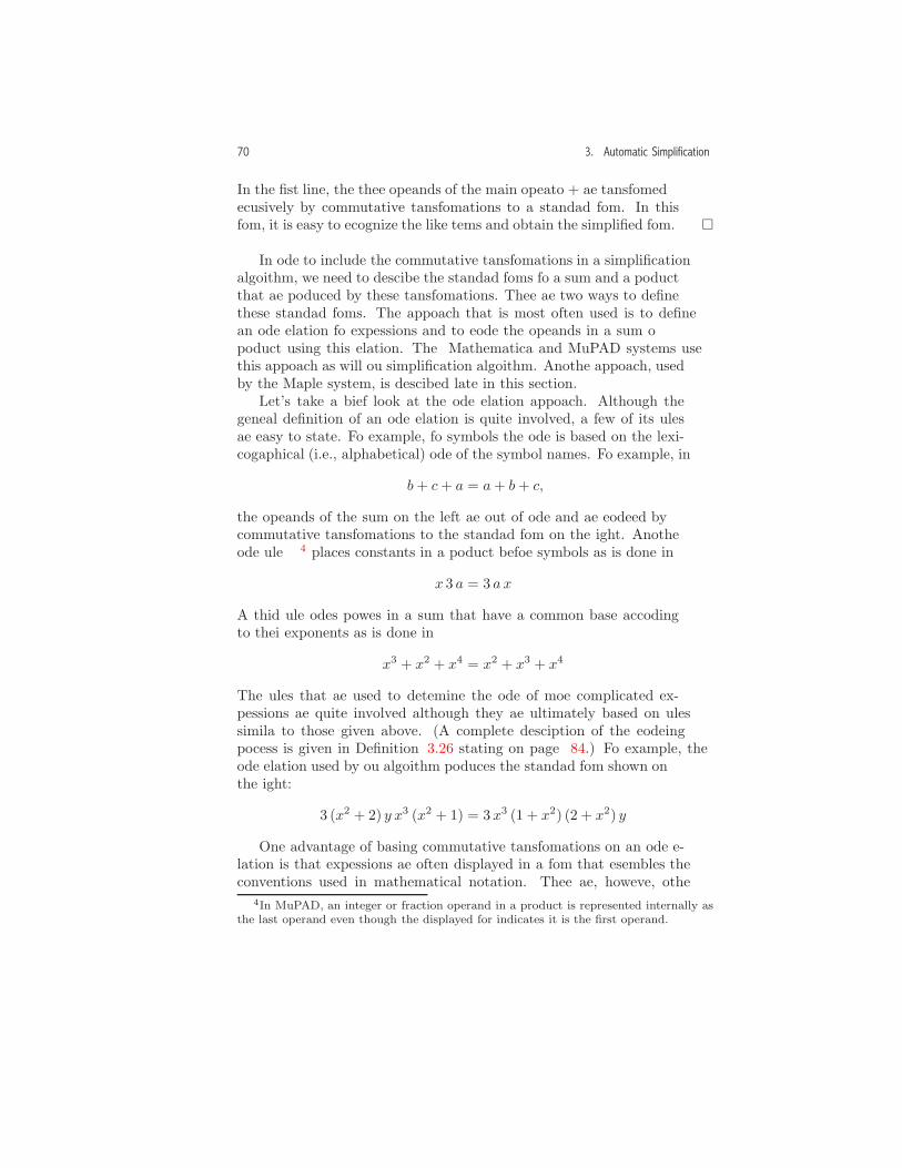
70 3. Automatic Simplification
In the first line, the three operands of the main operator + are transformedrecursively by commutative transformations to a standard form. In thisform, it is easy to recognize the like terms and obtain the simplified form. �
In order to include the commutative transformations in a simplificationalgorithm, we need to describe the standard forms for a sum and a productthat are produced by these transformations. There are two ways to definethese standard forms. The approach that is most often used is to definean order relation for expressions and to reorder the operands in a sum orproduct using this relation. The Mathematica and MuPAD systems usethis approach as will our simplification algorithm. Another approach, usedby the Maple system, is described later in this section.
Let’s take a brief look at the order relation approach. Although thegeneral definition of an order relation is quite involved, a few of its rulesare easy to state. For example, for symbols the order is based on the lexi-cographical (i.e., alphabetical) order of the symbol names. For example, in
b+ c+ a = a+ b+ c,
the operands of the sum on the left are out of order and are reordered bycommutative transformations to the standard form on the right. Anotherorder rule4 places constants in a product before symbols as is done in
x 3 a = 3 a x.
A third rule orders powers in a sum that have a common base accordingto their exponents as is done in
x3 + x2 + x4 = x2 + x3 + x4.
The rules that are used to determine the order of more complicated ex-pressions are quite involved although they are ultimately based on rulessimilar to those given above. (A complete description of the reorderingprocess is given in Definition 3.26 starting on page 84.) For example, theorder relation used by our algorithm produces the standard form shown onthe right:
3 (x2 + 2) y x3 (x2 + 1) = 3 x3 (1 + x2) (2 + x2) y.
One advantage of basing commutative transformations on an order re-lation is that expressions are often displayed in a form that resembles theconventions used in mathematical notation. There are, however, other
4In MuPAD, an integer or fraction operand in a product is represented internally asthe last operand even though the displayed form indicates it is the first operand.
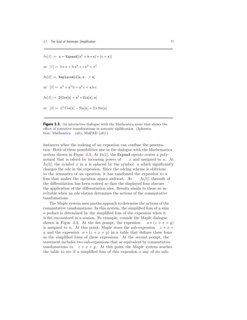
3.1. The Goal of Automatic Simplification 71
In[1 ] := u = Expand[(x2 + b ∗ x) ∗ (c + x)]
Out [1 ] = b c x + b x2 + c x2 + x3
In[2 ] := ReplaceAll[u, x− > a]
Out [2 ] = a3 + a2 b + a2 c + a b c
In[3 ] := D[Cos[x] + x2 ∗ Sin[x], x]
Out [3 ] = x2 Cos[x] − Sin[x] + 2 x Sin[x]
Figure 3.3. An interactive dialogue with the Mathematica system that shows theeffect of commutative transformations in automatic simplification. (Implementa-tion: Mathematica (nb), MuPAD (mnb).)
instances where the reordering of an expression can confuse the presenta-tion. Both of these possibilities arise in the dialogue with the Mathematicasystem shown in Figure 3.3. At In[1], the Expand operator creates a poly-nomial that is ordered by increasing powers of x and assigned to u. AtIn[2], the symbol x in u is replaced by the symbol a which significantlychanges the order in the expression. Since the ordering scheme is obliviousto the semantics of an operation, it has transformed the expression to aform that makes the operation appear awkward. At In[3], the result ofthe differentiation has been reordered so that the displayed form obscuresthe application of the differentiation rules. Results similar to these are in-evitable when an order relation determines the actions of the commutativetransformations.
The Maple system uses another approach to determine the actions of thecommutative transformations. In this system, the simplified form of a sumor product is determined by the simplified form of the expression when itis first encountered in a session. For example, consider the Maple dialogueshown in Figure 3.4. At the first prompt, the expression a ∗ (z + x + y)is assigned to u. At this point, Maple stores the sub-expression z + x +y and the expression a ∗ (z + x + y) in a table that defines these formsas the simplified forms of these expressions. At the second prompt, thestatement includes two sub-expressions that are equivalent by commutativetransformations to z + x + y. At this point the Maple system searchesthe table to see if a simplified form of this expression or any of its sub-

72 3. Automatic Simplification
> u := a*(z + x + y);
u := a (z + x+ y)
> v := b*(x + y + z) + c*(y + z + x);
v := b (z + x+ y) + c (z + x+ y)
> w := (3*z + 2*x + y - x - 2*z)*(x*x + a - x^2);
w := a (z + x+ y)
Figure 3.4. An interactive dialogue with the Maple system that illustrates theactions of the commutative transformations. (Implementation: Maple (mws).)
expressions can be transformed by commutative transformations to onealready in the table. Since z + x + y is already in the table, this form isused in the final simplified displayed expression. In a similar way, at thethird prompt an involved expression is simplified to a form that is alreadyin the table.
Each of the two approaches that determines the actions of the commu-tative transformations has its strengths and weaknesses. Let’s contrast thetwo approaches by comparing the Mathematica dialogue in Figure 3.3 to asimilar dialogue with the Maple system (Figure 3.5). The first statementin the Maple dialogue assigns an expression in powers of x to a variable u.However, in this case the simplified form is harder to comprehend than themore systematic form produced by the Mathematica system. On the otherhand, the next two Maple manipulations are much easier to follow thanthe Mathematica ones because the expressions are not reordered. The laststatement in the Maple session shows the sort operator which redefinesthe internal structure of a polynomial so that the powers now appear indecreasing order.
From a user’s perspective, it is difficult to make a general statementabout which of the two approaches produces more readable results. Ifexpressions are entered in the Maple system in a systematic way, there is agood chance the results will be displayed in a reasonable form. We didn’tdo this in the first statement in Figure 3.5 because x2+ b∗x has decreasingpowers of x while c+ x has increasing powers of x. If we had reversed the
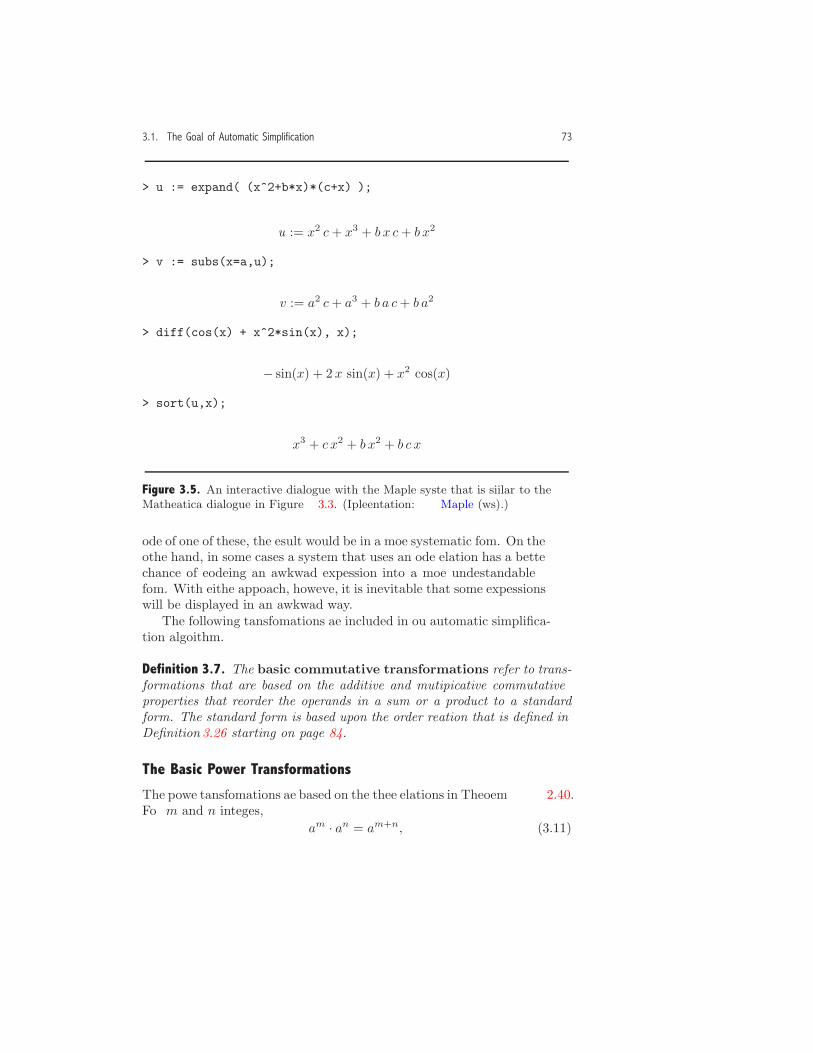
3.1. The Goal of Automatic Simplification 73
> u := expand( (x^2+b*x)*(c+x) );
u := x2 c+ x3 + b x c+ b x2
> v := subs(x=a,u);
v := a2 c+ a3 + b a c+ b a2
> diff(cos(x) + x^2*sin(x), x);
− sin(x) + 2 x sin(x) + x2 cos(x)
> sort(u,x);
x3 + c x2 + b x2 + b c x
Figure 3.5. An interactive dialogue with the Maple system that is similar to theMathematica dialogue in Figure 3.3. (Implementation: Maple (mws).)
order of one of these, the result would be in a more systematic form. On theother hand, in some cases a system that uses an order relation has a betterchance of reordering an awkward expression into a more understandableform. With either approach, however, it is inevitable that some expressionswill be displayed in an awkward way.
The following transformations are included in our automatic simplifica-tion algorithm.
Definition 3.7. The basic commutative transformations refer to trans-formations that are based on the additive and multiplicative commutativeproperties that reorder the operands in a sum or a product to a standardform. The standard form is based upon the order relation that is defined inDefinition 3.26 starting on page 84.
The Basic Power Transformations
The power transformations are based on the three relations in Theorem 2.40.For m and n integers,
am · an = am+n, (3.11)

74 3. Automatic Simplification
(am)n = am·n, (3.12)
(a · b)n = an · bn. (3.13)
In both the real field R and the complex field C, the power operation canbe generalized to allow exponents that are also members of the field. Inthese more general settings, the transformation (3.11) is true, while thetransformations (3.12) and (3.13) are only true when n is an integer (seeExample 3.11). With these considerations in mind, we assume that similartransformations are applied to mathematical expressions during automaticsimplification.
Definition 3.8. Let n be an integer. The following basic power transfor-mations are applied during automatic simplification:
uv · uw → uv+w, (3.14)
(uv)n → uv·n, (3.15)
(u · v)n → un · vn. (3.16)
As a result of these transformations, the simplified form of a power withan integer exponent cannot have a base that is also a power or a product.In addition, the simplified form of a product cannot have two operandsthat have a common base.
The power transformations in MPL are similar to those in Maple, Math-ematica, and MuPAD (Figure 3.6).
Example 3.9. Consider the simplification:
(x · y) · (x · y)2 = (x · y) · (x2 · y2)= x · y · x2 · y2
= x3y3.
In the first step, the second operand (x · y)2 is simplified (recursively)using the transformation (3.16). In the second step, a basic associativetransformation is applied to each operand of the main product. In thethird step, the transformation (3.14) is applied to give the final form.5
Notice how the associative transformation prepares the expression for thefinal power transformation. �
5Although the actual path taken by our algorithm for the last two steps is moreinvolved than what is shown in this example, the final result is the same.
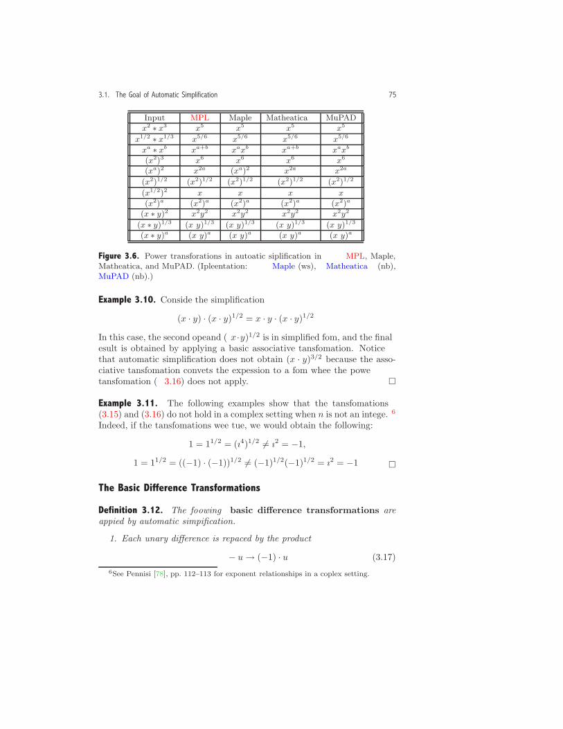
3.1. The Goal of Automatic Simplification 75
Input MPL Maple Mathematica MuPAD
x2 ∗ x3 x5 x5 x5 x5
x1/2 ∗ x1/3 x5/6 x5/6 x5/6 x5/6
xa ∗ xb xa+b xaxb xa+b xaxb
(x2)3 x6 x6 x6 x6
(xa)2 x2a (xa)2 x2a x2a
(x2)1/2 (x2)1/2 (x2)1/2 (x2)1/2 (x2)1/2
(x1/2)2 x x x x
(x2)a (x2)a (x2)a (x2)a (x2)a
(x ∗ y)2 x2y2 x2y2 x2y2 x2y2
(x ∗ y)1/3 (x y)1/3 (x y)1/3 (x y)1/3 (x y)1/3
(x ∗ y)a (x y)a (x y)a (x y)a (x y)a
Figure 3.6. Power transformations in automatic simplification in MPL, Maple,Mathematica, and MuPAD. (Implementation: Maple (mws), Mathematica (nb),MuPAD (mnb).)
Example 3.10. Consider the simplification
(x · y) · (x · y)1/2 = x · y · (x · y)1/2.In this case, the second operand (x ·y)1/2 is in simplified form, and the finalresult is obtained by applying a basic associative transformation. Noticethat automatic simplification does not obtain (x · y)3/2 because the asso-ciative transformation converts the expression to a form where the powertransformation (3.16) does not apply. �
Example 3.11. The following examples show that the transformations(3.15) and (3.16) do not hold in a complex setting when n is not an integer.6
Indeed, if the transformations were true, we would obtain the following:
1 = 11/2 = (ı4)1/2 �= ı2 = −1,1 = 11/2 = ((−1) · (−1))1/2 �= (−1)1/2(−1)1/2 = ı2 = −1. �
The Basic Difference Transformations
Definition 3.12. The following basic difference transformations areapplied by automatic simplification.
1. Each unary difference is replaced by the product
− u→ (−1) · u. (3.17)6See Pennisi [78], pp. 112–113 for exponent relationships in a complex setting.

76 3. Automatic Simplification
2. Each binary difference is replaced by the sum
u− v → u+ (−1) · v. (3.18)
As a result of these transformations, automatically simplified expres-sions do not contain the difference operator. Most computer algebra sys-tems apply these transformations during automatic simplification.
The Basic Quotient Transformation
Definition 3.13. During automatic simplification the following basic quo-tient transformation is applied:
u
v→ u · v−1. (3.19)
As a result of this transformation, automatically simplified expressionsdo not contain the quotient operator. Most computer algebra systems applythe quotient transformation during automatic simplification although thismay not be apparent from the displayed form of an expression which maystill contain a quotient operator.
Example 3.14. The quotient transformation prepares an expression for apower transformation as is done in
a · x3
x= (a · x3) · x−1 = a · x3 · x−1 = a · x2. �
The Basic Identity Transformations
Definition 3.15. The following basic identity transformations are ap-plied by automatic simplification:
u+ 0 → u, (3.20)u · 0 → 0, (3.21)u · 1 → u, (3.22)
0w →{ 0, if w is a positive integer or
fraction,Undefined, otherwise,
(3.23)
1w → 1, (3.24)

3.1. The Goal of Automatic Simplification 77
v0 →{1, if v �= 0,Undefined, if v = 0, (3.25)
v1 → v. (3.26)
In light of Definition 3.15, automatically simplified expressions satisfythe following properties.
1. A sum cannot have 0 as an operand.
2. A product cannot have 0 or 1 as an operand.
3. A power cannot have 0 or 1 as a base or an exponent.
The transformations (3.20)–(3.26) are considered basic because eachone appears in some form in our algorithm. Other manipulations involvingidentities are consequences of these basic identity transformations, numer-ical calculations with identity elements, and other transformations in thissection (Exercise 1, page 107). These include the following transformationswith quotients and differences:
u
0→ Undefined, (3.27)
0u→
{0, if u �= 0,Undefined, if u = 0, (3.28)
u/1 → u, (3.29)u− 0 → u, (3.30)0− u → (−1) · u. (3.31)
Although transformations similar to (3.20)–(3.31) are achieved by au-tomatic simplification in most computer algebra systems, some systemstransform powers with base 0 to other forms (see Figure 3.7). For exam-ple, although 00 is usually considered indeterminate, some mathematiciansdefine 00 as 1, and this transformation is obtained by both Maple and Mu-PAD.7 In addition, in MPL the expression 0w is considered undefined whenw is not a positive integer or fraction. Certainly, this is appropriate whenw is a negative integer or fraction, and when w is some other algebraic ex-pression, we take the conservative (safe) approach and simply assume thatthe expression is undefined. On the other hand, when w is not a non-zerointeger or fraction, Maple transforms 0w → 0, and both Mathematica andMuPAD consider 0w as an unevaluated power.
Unfortunately, since the transformations (3.23), (3.25), and (3.28) in-clude test conditions, they may give results that are not mathematically
7Knuth, Graham, and Patashnik [56] (page 162) assume that 00 = 1. Their motiva-tion is based on some limiting cases of the binomial theorem.

78 3. Automatic Simplification
MPL Maple Mathematica MuPAD00 Undefined 1 Indeterminate 10−2 Undefined error ComplexInfinity error
message message0w Undefined 0 0w 0w
Figure 3.7. Transformations of powers with base 0 in MPL, Maple, Mathemat-ica, and MuPAD. (Implementation: Maple (mws), Mathematica (nb), MuPAD(mnb).)
legitimate in a larger simplification context. For example, for the transfor-mation (
sin2(x) + cos2(x) − 1)0 → 1,
the base is not transformed to 0 by automatic simplification. Therefore,automatic simplification does not recognize this as the undefined expression00 and transforms it instead to 1.
The Basic Unary Transformations
Definition 3.16. The following basic unary transformations are appliedduring automatic simplification:
· x → x, (3.32)+x → x. (3.33)
These transformations apply to unary operations that appear in anexpression and to those that are created during the course of the simplifi-cation. As a result of these transformations, a simplified expression cannotcontain a unary product or sum.
The Basic Numerical Transformations
Definition 3.17. The following basic numerical transformations areapplied during automatic simplification:
1. the multiplication of constant operands in a product,
2. the addition of constant operands in a sum,
3. the evaluation of powers with an integer or fraction base and an in-teger exponent, and
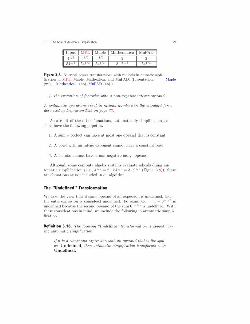
3.1. The Goal of Automatic Simplification 79
Input MPL Maple Mathematica MuPAD41/2 41/2 41/2 2 2541/3 541/3 541/3 3 · 21/3 541/3
Figure 3.8. Numerical power transformations with radicals in automatic simpli-fication in MPL, Maple, Mathematica, and MuPAD. (Implementation: Maple(mws), Mathematica (nb), MuPAD (mnb).)
4. the evaluation of factorials with a non-negative integer operand.
All arithmetic operations result in rational numbers in the standard formdescribed in Definition 2.25 on page 37.
As a result of these transformations, automatically simplified expres-sions have the following properties.
1. A sum or product can have at most one operand that is constant.
2. A power with an integer exponent cannot have a constant base.
3. A factorial cannot have a non-negative integer operand.
Although some computer algebra systems evaluate radicals during au-tomatic simplification (e.g., 41/2 = 2, 541/3 = 3 · 21/3 (Figure 3.8)), thesetransformations are not included in our algorithm.
The ”Undefined” Transformation
We take the view that if some operand of an expression is undefined, thenthe entire expression is considered undefined. For example, x + 0−1/2 isundefined because the second operand of the sum 0−1/2 is undefined. Withthese considerations in mind, we include the following in automatic simpli-fication.
Definition 3.18. The following “Undefined” transformation is applied dur-ing automatic simplification:
if u is a compound expression with an operand that is the sym-bol Undefined, then automatic simplification transforms u toUndefined.
80 3. Automatic Simplification
Basic Algebraic Expressions
In order to describe the automatic simplification algorithm, we need precisedefinitions for the expressions that are the input and output of the algo-rithm. The following definition describes the class of input expressions.
Definition 3.19. A basic algebraic expression (BAE) is an expressionthat satisfies one of the following rules.
BAE-1. u is an integer.
BAE-2. u is a fraction.
BAE-3. u is a symbol.
BAE-4. u is a product with one or more operands that are BAEs.
BAE-5. u is a sum with one or more operands that are BAEs.
BAE-6. u is a quotient with two operands that are BAEs.
BAE-7. u is a unary or binary difference where each operand is a BAE.
BAE-8. u is a power where both operands are BAEs.
BAE-9. u is a factorial with an operand that is a BAE.
BAE-10. u is a function form with one or more operands that are BAEs.
Example 3.20. The following are BAEs:
2/4, a · (x+ x), a+ b3/b, b− 3 · b, a+ (b + c) + d,
2 · 3 · x · x2, f(x)1, + x2 − x, 0−3, · x 2/(a− a), 3! �
The BAEs are similar to conventional algebraic expressions, except nowproducts and sums can have one or more operands. By including theseexpressions in the definition, the automatically simplified expressions (seeDefinition 3.21) are included in the BAEs. Notice that we have includedunary products as well as unary sums because they can be created in thecourse of a simplification. All unary products and sums are eliminatedduring the simplification process.
At this point, we allow expressions that are transformed by automaticsimplification to a mathematically undefined form because the algorithmrecognizes when these situations arise and returns the symbol Undefined.For example, in the last example, the expressions 0−3 and 2/(a − a) aremathematically undefined.
3.1. The Goal of Automatic Simplification 81
Automatically Simplified Algebraic Expressions
In Chapter 1 we described some of the structural properties of automat-ically simplified algebraic expressions. The next definition, which gives acomplete description of these expressions, defines the goal of automaticsimplification. The properties in the definition are the result of the basictransformations given in the beginning of this section.
Definition 3.21. An expression u is an automatically simplified alge-braic expression (ASAE) if it satisfies one of the following rules.
ASAE-1. u is an integer.
ASAE-2. u is a fraction in standard form.
ASAE-3. u is a symbol except the symbol Undefined.
The next rule describes the simplified form of a product. An importantsimplification transformation for products is the basic power transforma-tion uv · uw = uv+w. Since the relation holds when an exponent is un-derstood to be 1 (e.g., b · b2 = b3), it is useful to view each non-constantoperand of a product as a power. With these considerations in mind, wedefine the base and exponent of an ASAE u as
base(u) =
u, when u is a symbol, product, sum,factorial, or function
Operand(u, 1), when u is a power,Undefined, when u is an integer or fraction,
exponent(u) =
1, when u is a symbol, product, sum,
factorial, or function,Operand(u, 2), when u is a power,Undefined, when u is an integer or fraction.
For example,
base(x2) = x, exponent(x2) = 2,
base(x) = x, exponent(x) = 1.
The implementation of procedures for these operators is left to the reader(Exercise 1).
The base operator is used to define the simplified form of a product.

82 3. Automatic Simplification
ASAE-4. u is a product with two or more operands u1, u2, . . . , un thatsatisfy the following properties.
1. Each operand ui is an ASAE which can be either an integer ( �=0, 1), fraction, symbol (�= Undefined), sum, power, factorial,or function. (An operand of a product cannot be a product.) Anexpression that satisfies this property is called an admissiblefactor of a product.
2. At most one operand ui is a constant (integer or fraction).
3. If i �= j, then base(ui) �= base(uj).
4. If i < j, then ui✁uj.
The operator ✁ in ASAE-4-4 refers to the order relation on expressionsthat is used to define the actions of the commutative properties. Thedefinition of ✁ is given later in the section (see Definition 3.26 starting onpage 84).
Example 3.22. The expression 2 · x · y · z2 is a simplified product. Itcan be easily checked that this expression satisfies ASAE-4-1, ASAE-4-2,and ASAE-4-3, and once ✁ is defined, we shall see that it also satisfiesASAE-4-4. On the other hand, the following are not simplified:
2 · (x · y) · z2, (ASAE-4-1 is not satisfied),1 · x · y · z2, (ASAE-4-1 is not satisfied),2 · x · y · z · z2, (ASAE-4-3 is not satisfied). �
The next rule describes the simplified form of a sum. An importantsimplification transformation for a sum is the basic distributive transfor-mation that collects constant coefficients of like terms. In order to describethe result of this transformation, we need to precisely define “like term.”With this consideration in mind, we define the like-term part and constantpart of an ASAE u with the operators

3.1. The Goal of Automatic Simplification 83
term(u) =
·u, when u is a symbol, sum, power, factorial,or function,
u2 · · ·un, when u = u1 · · ·un is a productand u1 is constant,
u, when u = u1 · · ·un is a productand u1 is not constant,
Undefined, when u is an integer or fraction,
const(u) =
1, when u is a symbol, sum, power, factorial,or function,
u1, when u = u1 · · ·un is a productand u1 is constant,
1, when u = u1 · · ·un is a productand u1 is not constant,
Undefined, when u is an integer or fraction.
The definitions assume that a simplified product has at least two operands,and when a constant appears as an operand, it is the first operand.8 Ob-serve that when u is not an integer or fraction, the term operator returns aproduct with one or more operands. When the term operator is applied toan operand of a sum, it returns the part used to determine the like terms,while the const operator returns the corresponding coefficient part. Forexample,
term(x) = ·x, term(2 · y) = ·y, term(x · y) = x · y,
const(x) = 1, const(2 · y) = 2, const(x · y) = 1.
Notice that term(u) is either a product or Undefined. This means ex-pressions such as x and 2 · x have like-term parts that are structurally thesame. The implementation of procedures for these operators is left to thereader (Exercise 1).
The term operator is used to define the simplified form of a sum.
ASAE-5. u is a sum with two or more operands u1, u2, . . . , un that satisfythe following properties.
1. Each operand ui is an ASAE that can be either an integer ( �= 0),fraction, symbol (�= Undefined), product, power, factorial, orfunction. (An operand of a sum cannot a sum.) An expres-sion that satisfies this property is called an admissible term ofa sum.
2. At most one operand of u is a constant (integer or fraction).8See rule O-7 on page 87.
84 3. Automatic Simplification
3. If i �= j, then term(ui) �= term(uj).
4. If i < j, then ui✁uj.
Example 3.23. The sum 2 ·x+3 · y+4 · z is an ASAE. On the other hand,the following expressions are not simplified:
1 + (x + y) + z, (ASAE-5-1 is not satisfied),1 + 2 + x, (ASAE-5-2 is not satisfied),1 + x+ 2 · x, (ASAE-5-3 is not satisfied),z + y + x, (ASAE-5-4 is not satisfied). �
ASAE-6. u is a power vw that satisfies the following properties.
1. The expressions v and w are ASAEs.
2. The exponent w is not 0 or 1.
3. If w is an integer, then the base v is an ASAE which is asymbol(�= Undefined), sum, factorial, or function.
4. If w is not an integer, then the base v is any ASAE except 0or 1.
Example 3.24. The expressions x2, (1 + x)3, 2m, (x · y)1/2, and (x1/2)1/2
are ASAEs, while 23, (x2)3, (x y)2, (1 + x)1, and 1m are not. �
ASAE-7. u is a factorial with an operand that is any ASAE except anon-negative integer.
Example 3.25. The expressions n! and (−3)! are ASAEs, while 3! is not. �
ASAE-8. u is a function with one or more operands that are ASAEs.
The ✁ Order Relation
The ✁ order relation defines the actions of the basic commutative trans-formations, and, in a simplified sum or product, the operands are orderedaccording to this relation. Since the operands of these expressions are sim-plified recursively, it is sufficient to define the order relation for expressionsthat are automatically simplified.
Definition 3.26. Let u and v be distinct ASAEs. The ✁ order relation isdefined by the following rules.
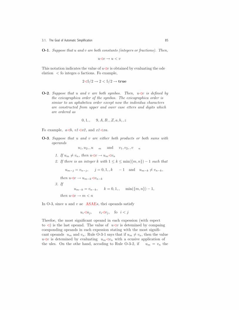
3.1. The Goal of Automatic Simplification 85
O-1. Suppose that u and v are both constants (integers or fractions). Then,
u✁v → u < v.
This notation indicates the value of u✁v is obtained by evaluating the orderrelation < for integers or fractions. For example,
2✁5/2→ 2 < 5/2→ true.
O-2. Suppose that u and v are both symbols. Then, u✁v is defined bythe lexicographical order of the symbols. The lexicographical order issimilar to an alphabetical order except now the individual charactersare constructed from upper and lower case letters and digits whichare ordered as
0, 1, . . . , 9, A,B, . . . , Z, a, b, . . . , z.
For example, a✁b, v1✁v2 , and x1✁xa.
O-3. Suppose that u and v are either both products or both sums withoperands
u1, u2, . . . , um and v1, v2, . . . , vn.
1. If um �= vn, then u✁v → um✁vn.
2. If there is an integer k with 1 ≤ k ≤ min({m,n})− 1 such that
um−j = vn−j , j = 0, 1, . . . , k − 1 and um−k �= vn−k,
then u✁v → um−k✁vn−k.
3. Ifum−k = vn−k, k = 0, 1, . . . ,min({m,n})− 1,
then u✁v → m < n.
In O-3, since u and v are ASAEs, their operands satisfy
ui✁uj, vi✁vj , for i < j.
Therefore, the most significant operand in each expression (with respectto ✁) is the last operand. The value of u✁v is determined by comparingcorresponding operands in each expression starting with the most signifi-cant operands um and vn. Rule O-3-1 says that if um �= vn, then the valueu✁v is determined by evaluating um✁vn with a recursive application ofthe rules. On the other hand, according to Rule O-3-2, if um = vn the

86 3. Automatic Simplification
focus shifts one operand to the left to um−1 and vn−1, and if um−1 �= vn−1,then u✁v = um−1✁vn−1. Again, if um−1 = vn−1, the focus shifts onemore step to the left to um−2 and vn−2. This process continues until ei-ther two unequal operands are found (say um−k �= vn−k) in which caseu✁v → um−k✁vn−k, or until either u or v runs out of operands in whichcase condition O-3-3 applies. For example,
a+ b✁a+ c, a+ c+ d✁b+ c+ d, c+ d✁b+ c+ d.
O-4. Suppose that u and v are both powers.
1. If base(u) �= base(v), then
u✁v → base(u)✁base(v).
2. If base(u) = base(v), then
u✁v → exponent(u)✁exponent(v).
In other words, if the bases are different, the order is determined by theorder of bases, and if the bases are the same, the order is determined bythe order of the exponents.
Example 3.27. Using O-4, O-1, and O-3-1, we have
(1 + x)2✁(1 + x)3✁(1 + y)2. (3.34)
�
O-5. If u and v are both factorials, then
u✁v → Operand(u, 1)✁Operand(v, 1).
The order of two factorials is obtained by comparing their operands.
O-6. Suppose that u and v are functions.
1. If Kind(u) �= Kind(v), then u✁v → Kind(u)✁Kind(v).2. Suppose that Kind(u) = Kind(v), and the operands of the func-
tions are given by u1, u2, . . . , um and v1, v2, . . . , vn.
(a) If u1 �= v1, then u✁v → u1✁v1.
(b) If there is an integer k with 1 ≤ k ≤ min({m,n}) such that
uj = vj , j = 1, . . . , k − 1 and uk �= vk,
then u✁v → uk✁vk.

3.1. The Goal of Automatic Simplification 87
(c) Ifuk = vk, k = 1, . . . ,min({m,n}),
then u✁v → m < n.
When two functions have different names, the order is determined by thefunction names. For example, f(x)✁g(x). The comparison of functionswith the same name is similar to the comparison of two products or twosums, except now the first operand is the most significant operand. Forexample, f(x)✁f(y) and g(x)✁g(x, y).
The rules given so far apply when either u and v are both constants orKind(u) = Kind(v). The remaining rules apply when u and v are differenttypes.
O-7. If u is an integer or fraction and v is any other type, then u✁v.
As a consequence of this rule, whenever a constant is an operand in asimplified sum or product, it must be the first operand.
O-8. Suppose that u is a product. If v is a power, sum, factorial, function,or symbol, then9
u✁v → u✁ · v. (3.35)
In other words, in this rule the order is determined by viewing both expres-sions as products and recursively applying O-3. Notice that we streamlinethe rule list by not mentioning explicitly the case where u is a productand v a constant because this is handled through rule O-13, where u andv are interchanged together with a recursive application of O-7. For theremaining rules, we omit cases that are handled by earlier rules throughrule O-13.
Example 3.28. This rule is a natural way to compare a product and apower because it implies that an expression like a · x2 + x3 with increasing
9Strictly speaking, � is only defined for automatically simplified expressions. Al-though the expression ·v in this rule is not automatically simplified, the order u � · v isstill well defined because it simply provides a way to compare the last operand of u tov. In fact, the rule can be defined without the unary product. If u = u1 · · · un, then thetransformation (3.35) is equivalent to
u � v → un � v, if un �= v,true, if un = v.
We use the unary product form of the rule, however, because the rules are somewhat eas-ier to describe in this format. These comments also apply to rules O-9, O-10, and O-11.

88 3. Automatic Simplification
powers of x is an ASAE. Indeed, using O-8 followed by O-3-1, O-4-2, andO-1, we have
a · x2✁x3 → a · x2✁ · x3 → x2✁x3 → 2 < 3→ true. �
O-9. Suppose that u is a power. If v is a sum, factorial, function, orsymbol, then
u✁v → u✁v1.
In other words, in this rule the order is determined by viewing both ex-pressions as powers and recursively applying rule O-4.
Example 3.29. Using O-9 followed by O-4-1, O-3-2, and O-2, we have
(1 + x)3✁(1 + y)→ (1 + x)3✁(1 + y)1 → (1 + x)✁(1 + y)→ x✁y → true.
�
O-10. Suppose that u is a sum. If v is a factorial, function, or symbol,then
u✁v → u✁+ v.
In other words, in this rule the order is determined by viewing both ex-pressions as sums and recursively applying rule O-3.
Example 3.30. Using O-10, O-3-1, and O-2, we have 1 + x✁y. �
O-11. Suppose that u is a factorial. If v is a function or symbol, then
1. If Operand(u, 1) = v then u✁v → false.2. If Operand(u, 1) �= v then u✁v → u✁v!.
In other words when Operand(u, 1) �= v, the order is determined by viewingboth expressions as factorials and then recursively applying rule O-5. Forexample, this rule implies m!✁n.
O-12. Suppose that u is a function, and v is a symbol.
1. If Kind(u) = v, then u✁v → false.2. If Kind(u) �= v, then u✁v → Kind(u)✁v.
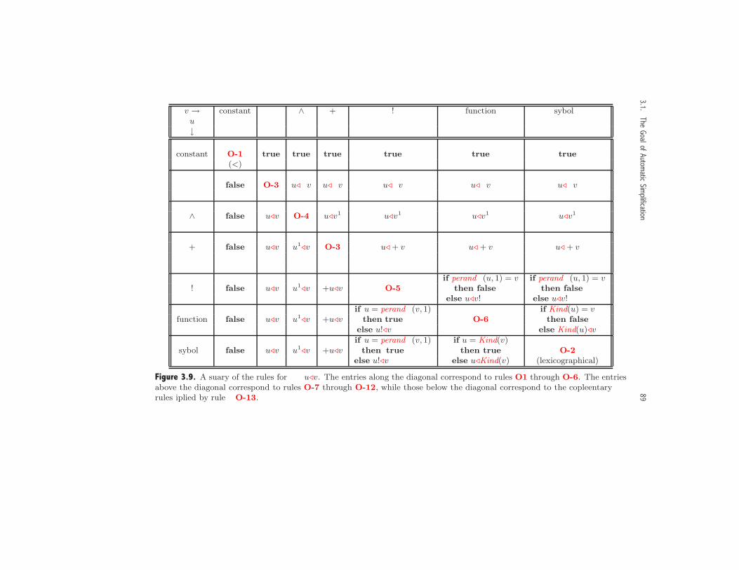
3.1.The
GoalofAutomatic
Simplification
89
v → constant · ∧ + ! function symbolu↓
constant O-1 true true true true true true(<)
· false O-3 u( · v u( · v u( · v u( · v u( · v
∧ false ·u(v O-4 u(v1 u(v1 u(v1 u(v1
+ false ·u(v u1(v O-3 u( + v u( + v u( + v
if Operand(u, 1) = v if Operand(u, 1) = v! false ·u(v u1(v +u(v O-5 then false then false
else u(v! else u(v!
if u = Operand(v, 1) if Kind(u) = vfunction false ·u(v u1(v +u(v then true O-6 then false
else u!(v else Kind(u)(v
if u = Operand(v, 1) if u = Kind(v)symbol false ·u(v u1(v +u(v then true then true O-2
else u!(v else u(Kind(v) (lexicographical)
Figure 3.9. A summary of the rules for u(v. The entries along the diagonal correspond to rules O1 through O-6. The entriesabove the diagonal correspond to rules O-7 through O-12, while those below the diagonal correspond to the complementaryrules implied by rule O-13.

90 3. Automatic Simplification
Example 3.31. Rule O-12-1 implies x✁x(t), and Rules O-12-2 and O-2imply x✁y(t). �
O-13. If u and v do not satisfy the conditions in any of the above rules,then
u✁v → not(v✁u).
Example 3.32. If u = x and v = x2, then the first 12 rules do not apply.However, using rules O-13, O-9, O-4-2, and O-1, we have
x✁x2 → not(x2✁x)→ not(x2✁x1)→ not(2 < 1)→ not(false)→ true.�
A summary of the ✁ rules, which includes the complementary rulesimplied by O-13, is given in Figure 3.9.
The ✁ transformation rules can be readily expressed in a procedurethat determines the order of two expressions. The details of the procedureare left to the reader (Exercise 2).
Exercises1. Let u be an ASAE in function notation. Give a procedure for each of the
following operators.
(a) An operator Base(u) for base(u).
(b) An operator Exponent(u) for exponent(u).
(c) An operator Term(u) for term(u).
(d) An operator Const(u) for const(u).
These operators are used in the automatic simplification algorithm de-scribed in Section 3.2.
2. Let u and v be ASAEs in function notation. Give a procedure
Compare(u, v)
that evaluates the order relation u ( v. The operator returns true whenu ( v and false otherwise. Note: To obtain the order of two symbolsthe following commands can be used: in Maple, the lexorder com-mand; in Mathematica, the Order command; and in MuPAD, the sysordercommand. (Implementation: Maple (mws), Mathematica (nb), MuPAD(mnb).)
This operator is used in the automatic simplification algorithm describedin Section 3.2.
3. Let u be a BAE in function notation. Give a procedure ASAE (u) thatreturns true if u is an ASAE and false otherwise.

3.2. An Automatic Simplification Algorithm 91
4. Determine u ( v for each of the following pairs of expressions. In each case,give the sequence of rules used to determine u ( v.
(a) u = a + b, v = c.
(b) u = a · b, v = a + b2.
(c) u = c2, v = a + b4.
(d) u = (2 + 4 · x)3, v = y2.
(e) u = c · (x + 4 · y2), v = (a + 3 · b2) · (x + 4 · y2).
5. Give the automatically simplified form of each of the following expressions.Indicate which simplification rules are applied to determine the simplifiedform.
(a) m · c2.
(b)m · v2
2.
(c) a · x2 + b · x + c.
(d) ((x1/2)1/2)8.
(e) ((x · y)1/2 · z2)2.
6. Show that each of the following expressions is an ASAE.
(a) 1 + x + 2 · (1 + x).
(b) x2 · (x2)y .
(c) 3 · x3 · (1 + x2) · (2 + x2) · y.
3.2 An Automatic Simplification Algorithm
In this section we describe an automatic simplification algorithm that isbased on the basic algebraic transformations described in Section 3.1. Thealgorithm does the following:
1. For u a BAE, the algorithm returns either an ASAE or the symbolUndefined.
2. For u an ASAE, the algorithm returns u.
The Main Simplification Procedure
The main procedure of the algorithm is given in Figure 3.10. In order tobypass a CAS’s automatic simplification process, we assume that the inputexpression is in function notation (see Figure 2.6, page 39) instead of infixnotation. For clarity, however, we use infix notation in our discussion andexamples.

92 3. Automatic Simplification
Procedure Automatic simplify(u);Inputu : a BAE in function notation;
OutputAn ASAE in function notation or the symbol Undefined;
Local Variablesv;
Begin1 if Kind(u) ∈ {integer, symbol} then2 Return(u);3 elseif Kind(u) = FracOp then4 Return(Simplify rational number(u))5 else6 v := Map(Automatic simplify, u);7 if Kind(v) = PowOp then8 Return(Simplify power(v))9 elseif Kind(v) = ProdOp then10 Return(Simplify product(v))11 elseif Kind(v) = SumOp then12 Return(Simplify sum(v))13 elseif Kind(v) = QuotOp then14 Return(Simplify quotient(v))15 elseif Kind(v) = DiffOp then16 Return(Simplify difference(v))17 elseif Kind(v) = FactOp then18 Return(Simplify factorial(v))19 else20 Return(Simplify function(v))
End
Figure 3.10. The main MPL procedure in the Automatic simplify algorithm.(Implementation: Maple (txt), Mathematica (txt), MuPAD (txt).)
To begin, since integers and symbols are in simplified form, the pro-cedure simply returns the input expression (lines 1–2). For fractions, thesimplified form is obtained (at line 4) with the Simplify rational numberprocedure described in Section 2.2. For other compound expressions, wefirst recursively simplify the operands (line 6) and then apply the appro-priate simplification operator (lines 7–20).
Because of the large number of basic transformations described in Sec-tion 3.1 and the complex interactions between them, the automatic simpli-fication algorithm is quite involved. In Figure 3.11, we list the operators
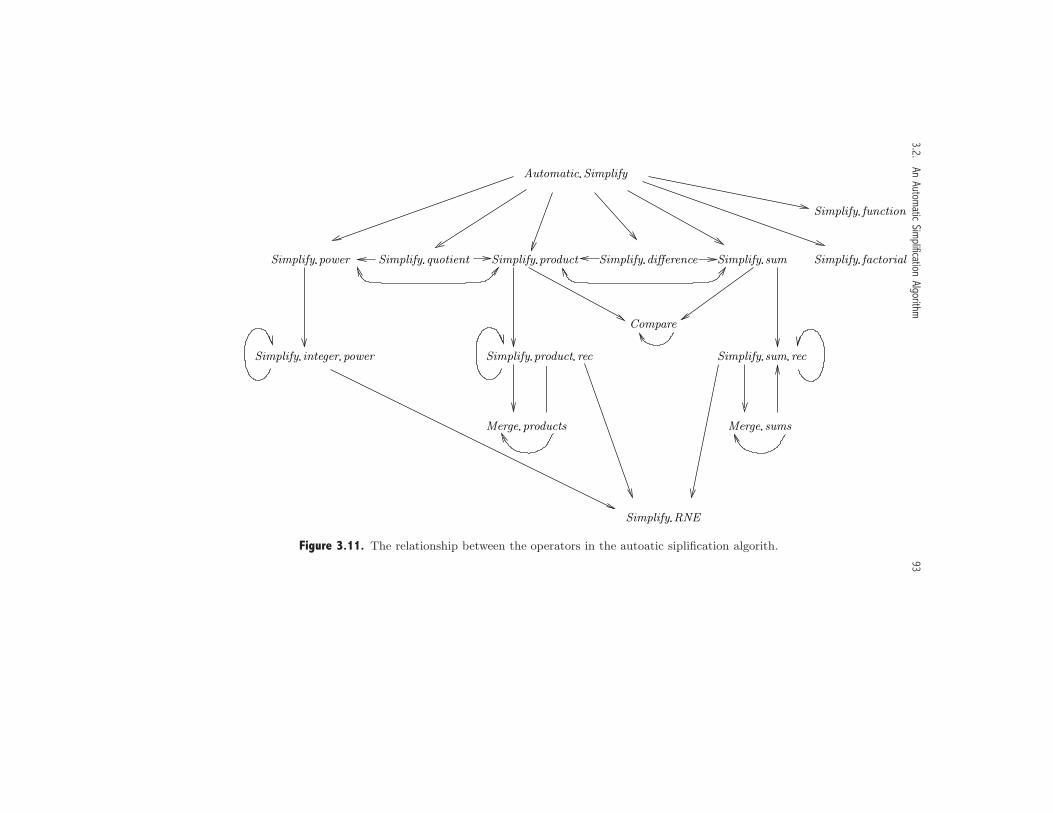
3.2.AnAutom
aticSimplification
Algorithm93
Simplify product rec
Merge products
Automatic Simplify
Simplify product Simplify difference
Simplify function
Simplify sum Simplify factorialSimplify quotientSimplify power
Simplify RNE
Simplify sum rec
Merge sums
Simplify integer power
Compare
Figure 3.11. The relationship between the operators in the automatic simplification algorithm.

94 3. Automatic Simplification
called by Automatic simplify along with other operators that make up thealgorithm. An arrow from one operator to another operator indicates thatthe first operator calls on the second operator, and a circular referenceindicates the operator is recursive. Each of the operators is defined by acollection of transformation rules, and in order to guide the reader throughthe maze of rules, we give a large number of examples to illustrate how therules are applied.
Simplification of Powers
The Simplify power operator, which transforms a power vw to either anASAE or the symbol Undefined, is based on the following transforma-tions:
1. the basic power transformations (3.15) and (3.16),
2. the basic identity transformations (3.23), (3.24), (3.25), and (3.26),
3. the basic numerical transformation in Definition 3.17(3), and
4. the “Undefined” transformation in Definition 3.18.
The operator is defined in terms of a main sequence of non-recursive trans-formation rules (Definition 3.33) which calls on another sequence of recur-sive rules (Definition 3.34).
Definition 3.33. Let u = vw where the base v = Operand(u, 1) and theexponent w = Operand(u, 2) are either ASAEs or the symbol Undefined.The operator Simplify power(u) is defined by the following transformationrules.
SPOW-1. If v = Undefined or w = Undefined then
Simplify power (u)→ Undefined.
SPOW-2. Suppose that v = 0. If w is a positive integer or fraction, then
Simplify power (u)→ 0,
otherwiseSimplify power (u)→ Undefined.
SPOW-3. If v = 1, then
Simplify power (u)→ 1.

3.2. An Automatic Simplification Algorithm 95
SPOW-4. If w is an integer, then
Simplify power (u)→ Simplify integer power(v, w).
(Simplify integer power is defined in Definition 3.34 below.)
SPOW-5. If the first four rules do not apply, then
Simplify power (u)→ u.
Rule SPOW-1 states that a power with anUndefined operand inheritsthis Undefined value. This happens, for example, with (1/0)2 because thesimplified form of the base is Undefined.
Rules SPOW-2 and SPOW-3 are the basic identity transformations(3.23) and (3.24). Rule SPOW-4, which simplifies powers with integerexponents, is defined by the Simplify integer power operator (see Defini-tion 3.34 below). The last rule SPOW-5, which handles all other cases,simply returns u without change.
Definition 3.34. Consider the expression vn where v �= 0 is an ASAE andn is an integer. The operator Simplify integer power(v, n) is defined by thefollowing transformation rules.
SINTPOW-1. If Kind(v) ∈ {integer,FracOp}, then
Simplify integer power (v, n)→ Simplify RNE(PowOp(v, n)).
Rule SINTPOW-1, performs the numerical computation of powers usingthe Simplify RNE operator described in Section 2.2.
SINTPOW-2. If n = 0, then Simplify integer power(v, n)→ 1.
SINTPOW-3. If n = 1, then Simplify integer power(v, n)→ v.
Rules SINTPOW-2, and SINTPOW-3, achieve the two basic identity trans-formations (3.25) and (3.26). In SINTPOW-2, since SPOW-2 above isapplied before this rule, we assume that v �= 0.
SINTPOW-4. Suppose that Kind(v) = PowOp with base
r = Operand(v, 1)
and exponents = Operand(v, 2).
In addition, let
p = Simplify product(ProdOp(s, n)). (3.36)
(Simplify product is given in Definition 3.37.)
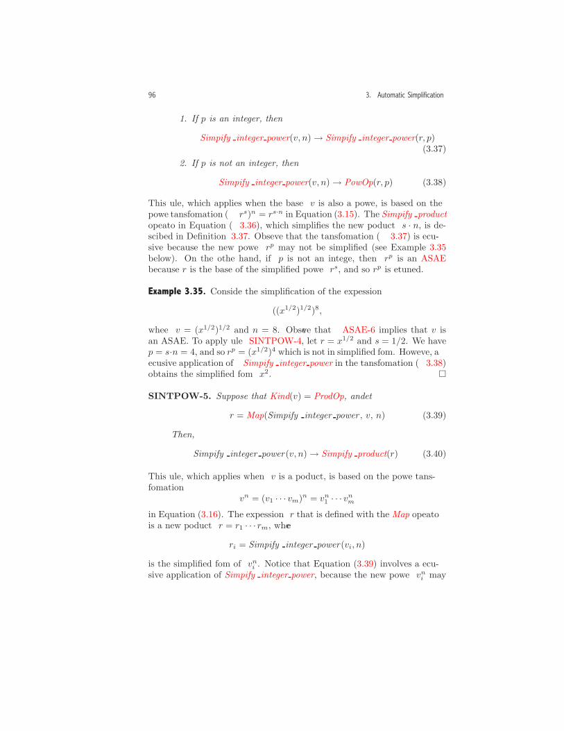
96 3. Automatic Simplification
1. If p is an integer, then
Simplify integer power(v, n)→ Simplify integer power(r, p).(3.37)
2. If p is not an integer, then
Simplify integer power(v, n)→ PowOp(r, p). (3.38)
This rule, which applies when the base v is also a power, is based on thepower transformation (rs)n = rs·n in Equation (3.15). The Simplify productoperator in Equation (3.36), which simplifies the new product s · n, is de-scribed in Definition 3.37. Observe that the transformation (3.37) is recur-sive because the new power rp may not be simplified (see Example 3.35below). On the other hand, if p is not an integer, then rp is an ASAEbecause r is the base of the simplified power rs, and so rp is returned.
Example 3.35. Consider the simplification of the expression
((x1/2)1/2)8,
where v = (x1/2)1/2 and n = 8. Observe that ASAE-6 implies that v isan ASAE. To apply rule SINTPOW-4, let r = x1/2 and s = 1/2. We havep = s·n = 4, and so rp = (x1/2)4 which is not in simplified form. However, arecursive application of Simplify integer power in the transformation (3.38)obtains the simplified form x2. �
SINTPOW-5. Suppose that Kind(v) = ProdOp, and let
r = Map(Simplify integer power , v, n). (3.39)
Then,
Simplify integer power (v, n)→ Simplify product(r). (3.40)
This rule, which applies when v is a product, is based on the power trans-formation
vn = (v1 · · · vm)n = vn1 · · · vnmin Equation (3.16). The expression r that is defined with the Map operatoris a new product r = r1 · · · rm, where
ri = Simplify integer power (vi, n)
is the simplified form of vni . Notice that Equation (3.39) involves a recur-sive application of Simplify integer power, because the new power vni may

3.2. An Automatic Simplification Algorithm 97
not be in simplified form. In addition, since the new product r may notbe in simplified form, it is simplified in transformation (3.40) with theSimplify product operator. These points are illustrated in Example 3.36.
Example 3.36. Consider the simplification of((x · y)1/2 · z2
)2
,
wherev = v1 v2 = (x · y)1/2 · z2, n = 2.
Then,
r = Simplify integer power((x · y)1/2 , 2
)· Simplify integer power
(z2, 2
)→ (x · y) · z4. (3.41)
Notice that the expression (3.41) is not a simplified product because of theparentheses about x · y. Using the transformation (3.40), we obtain thesimplified form
Simplify product(r)→ x · y · z4. �
SINTPOW-6. If none of the rules apply, then
Simplify integer power (v, n)→ PowOp(v, n).
The last rule applies when v is a symbol, sum, factorial, or function.In this rule, vn is already simplified, and so this expression is returned infunction notation.
Simplification of Products
The Simplify product operator, which transforms a product to either anASAE or the symbolUndefined, is based on the following transformations:
1. the basic associative transformation (Definition 3.5(2)),
2. the basic commutative transformation for products (Definition 3.7),
3. the basic power transformation (3.14),
4. the basic identity transformations (3.21) and (3.22),
5. the basic unary transformation (3.32),
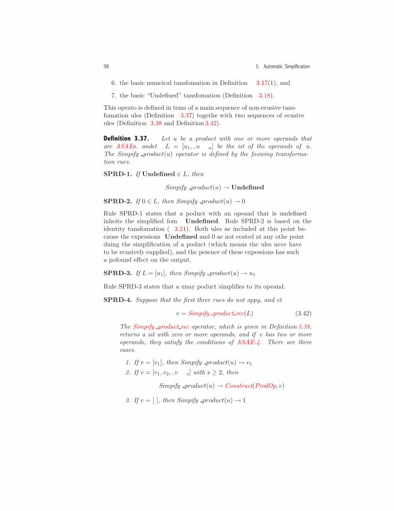
98 3. Automatic Simplification
6. the basic numerical transformation in Definition 3.17(1), and
7. the basic “Undefined” transformation (Definition 3.18).
This operator is defined in terms of a main sequence of non-recursive trans-formation rules (Definition 3.37) together with two sequences of recursiverules (Definition 3.38 and Definition 3.42).
Definition 3.37. Let u be a product with one or more operands thatare ASAEs, and let L = [u1, . . . , un] be the list of the operands of u.The Simplify product(u) operator is defined by the following transforma-tion rules.
SPRD-1. If Undefined ∈ L, then
Simplify product(u)→ Undefined.SPRD-2. If 0 ∈ L, then Simplify product(u)→ 0.
Rule SPRD-1 states that a product with an operand that is undefinedinherits the simplified form Undefined. Rule SPRD-2 is based on theidentity transformation (3.21). Both rules are included at this point be-cause the expressions Undefined and 0 are not created at any other pointduring the simplification of a product (which means the rules never haveto be recursively reapplied), and the presence of these expressions has sucha profound effect on the output.
SPRD-3. If L = [u1], then Simplify product(u)→ u1.
Rule SPRD-3 states that a unary product simplifies to its operand.
SPRD-4. Suppose that the first three rules do not apply, and let
v = Simplify product rec(L). (3.42)
The Simplify product rec operator, which is given in Definition 3.38,returns a list with zero or more operands, and if v has two or moreoperands, they satisfy the conditions of ASAE-4. There are threecases.
1. If v = [v1], then Simplify product(u)→ v1.
2. If v = [v1, v2, . . . , vs] with s ≥ 2, then
Simplify product(u)→ Construct(ProdOp, v).
3. If v = [ ], then Simplify product(u)→ 1.

3.2. An Automatic Simplification Algorithm 99
Rule SPRD-4-1 is invoked when the operands of u simplify to a productwith single operand v1, in which case the simplified form is just the operandv1. For example, using the rules in Definition 3.38 and Definition 3.42, wehave
v = Simplify product rec([a−1, b, a])→ [b],
and therefore by SPRD-4-1,
Simplify product(a−1 · b · a)→ b.
Rule SPRD-4-2 corresponds to the case where the simplified form of aproduct is also a product. For example, since
v = Simplify product rec([c, 2, b, c, a])→ [2, a, b, c2],
we haveSimplify product(c · 2 · b · c · a)→ 2 · a · b · c2.
Rule SPRD 4-3 is included since an integer 1 that is created during thesimplification of a product is not included in the operand list (see rulesSPRDREC-1-1 and SPRDREC-1-3). (It is convenient to do this becauseASAE-4-1 states that an operand of a simplified product cannot be theinteger 1.) For this reason, Simplify product rec(L) may return the emptylist, and when this happens, the product simplifies to 1 (see Example 3.39).
Definition 3.38. Let L = [u1, u2, . . . , un] be a non-empty list with n ≥ 2non-zero ASAEs. The operator Simplify product rec(L) (for “Simplify prod-uct recursive”) returns a list with zero or more operands. The operator isdefined by the following transformation rules.
SPRDREC-1. Suppose that L = [u1, u2] and neither operand is a product.
1. Suppose that both u1 and u2 are constants, and let
P = Simplify RNE(ProdOp(u1, u2)).
If P = 1, then
Simplify product rec(L)→ [ ],
and if P �= 1, then
Simplify product rec(L)→ [P ].
2. (a) If u1 = 1, then Simplify product rec(L)→ [u2].(b) If u2 = 1, then Simplify product rec(L)→ [u1].

100 3. Automatic Simplification
3. Suppose that base(u1) = base(u2), and let
S = Simplify sum(SumOp(exponent(u1), exponent(u2)))
andP = Simplify power(PowOp(base(u1), S)).
If P = 1, then
Simplify product rec(L)→ [ ],
and if P �= 1, then
Simplify product rec(L)→ [P ].
4. If u2✁u1, then
Simplify product rec(L)→ [u2, u1].
5. If the first four rules do not apply, then
Simplify product rec(L)→ L.
Rule SPRDREC-1 applies when L has two operands and neither one is aproduct. (The case when one of the operands is a product is handled in ruleSPRDREC-2.) Rule SPRDREC-1-1 is the basic numerical transformationin Definition 3.17(1). Observe that when the product P = 1, the emptylist is returned. This is done so that the integer 1 created during thesimplification process is not included as an operand of a product (see alsorules SPRD-4-3 and SPRDREC-1-3).
Rule SPRDREC-1-2 is based on the basic identity transformation (3.22).Rule SPRDREC-1-3 performs the basic power transformation (3.14).
The Simplify sum operator (Exercise 7) simplifies the sum of the expo-nents, and since the new power may not be an ASAE, the rule includes anapplication of Simplify power. Again, when the product P = 1, the emptylist is returned.
Example 3.39. If L = [a, a−1], then S = 0 and aS = a0, which is not insimplified form. Applying the Simplify power operator, we have P = 1 andso Simplify product rec([a, a−1])→ [ ]. �
Rule SPRDREC-1-4 is invoked when the two operands are out of orderwith respect to the ✁ order relation. When the last rule SPRDREC-1-5 isinvoked, the earlier conditions that lead to a modification of the input donot apply, and so the input is returned without change.

3.2. An Automatic Simplification Algorithm 101
SPRDREC-2. Suppose that L = [u1, u2], and suppose that at least one ofits two operands is a product.
1. If u1 is a product with operands p1, p2, . . . , ps and u2 is a productwith operands q1, q2, . . . , qt, then
Simplify product rec(L)→Merge products([p1, p2, . . . , ps], [q1, q2, . . . , qt]).
(Merge products is given in Definition 3.42.)2. If u1 is a product with operands
p1, p2, . . . , ps
and u2 is not a product, then
Simplify product rec(L)→ Merge products([p1, p2, . . . , ps], [u2]).
3. If u1 is not a product and u2 is a product with operands
q1, q2, . . . , qt,
then
Simplify product rec(L)→ Merge products([u1], [q1, q2, . . . , qt]).
Rule SPRDREC-2, which is based on the basic associative transforma-tion in Definition 3.5(2), applies when L has two operands and at leastone operand is a product. This rule (together with SPRDREC-3) guar-antees that a simplified product will not have an operand that is also aproduct. The Merge products operator, which is given in Definition 3.42,applies the associative property and combines and re-orders the operandsof the two products to create a new operand list. This rule is recursivebecause Merge products invokes one of the earlier SPRDREC rules.
Example 3.40. To simplify the expression u = (2 · a · c · e) · (3 · b · d · e), wehave by SPRDREC-2-(a)
Simplify product rec([2 · a · c · e, 3 · b · d · e])→ Merge products([2, a, c, e], [3, b, d, e])→ [6, a, b, c, d, e2].
Therefore, the original expression u simplifies to 6 · a · b · c · d · e2. �
In SPRDREC-2-2 and SPRDREC-2-3, only one of the operands is aproduct, and so the remaining operand (u2 or u1) is merged with theoperands of the product (p1, . . . , ps or q1, . . . , qt).

102 3. Automatic Simplification
SPRDREC-3. Suppose that L = [u1, u2, . . . , un] with n > 2, and let
w = Simplify product rec(Rest(L)). (3.43)
1. If u1 is a product with operands p1, p2, . . . , ps, then
Simplify product rec(L)→ Merge products([p1, p2, . . . , ps], w).
2. If u1 is not a product, then
Simplify product rec(L)→ Merge products([u1], w).
Rule SPRDREC-3 is invoked when the input list L has more than twooperands. The first rule SPRDREC-3-1 is similar to the associative trans-formation SPRDREC-2-1. It merges the operands of the product u1 withthe list of operands that make up the simplified form of Rest(L). In asimilar way, rule SPRDREC-3-2 merges the single operand u1 with theoperands of w.
Example 3.41. Suppose that L = [a · b, c, b]. Then, applying the rulesSPRDREC-3-1 and SPRDREC-1-4, we have
w = Simplify product rec([c, b])→ [b, c].
Therefore,
Simplify product rec([a · b, b, c]) = Merge products([a, b], [b, c])→ [a, b2, c]. �
The transformation rules for Merge products(p, q) are given in the nextdefinition. When
p = [p1, . . . , pm], q = [q1, . . . , qn]
represent the operands of two simplified products, the operator applies thebasic product associative transformation and, using Simplify product rec,combines and reorders the operands of p and q into a new operand list.
Definition 3.42. Let p and q be lists of zero or more admissible factors in ✁
order. In addition, if p or q has two or more operands, the operands satisfythe properties of ASAE-4. The operator Merge products(p, q) is definedusing the following rule sequence:
MPRD-1. If q = [ ], then Merge products(p, q)→ p.
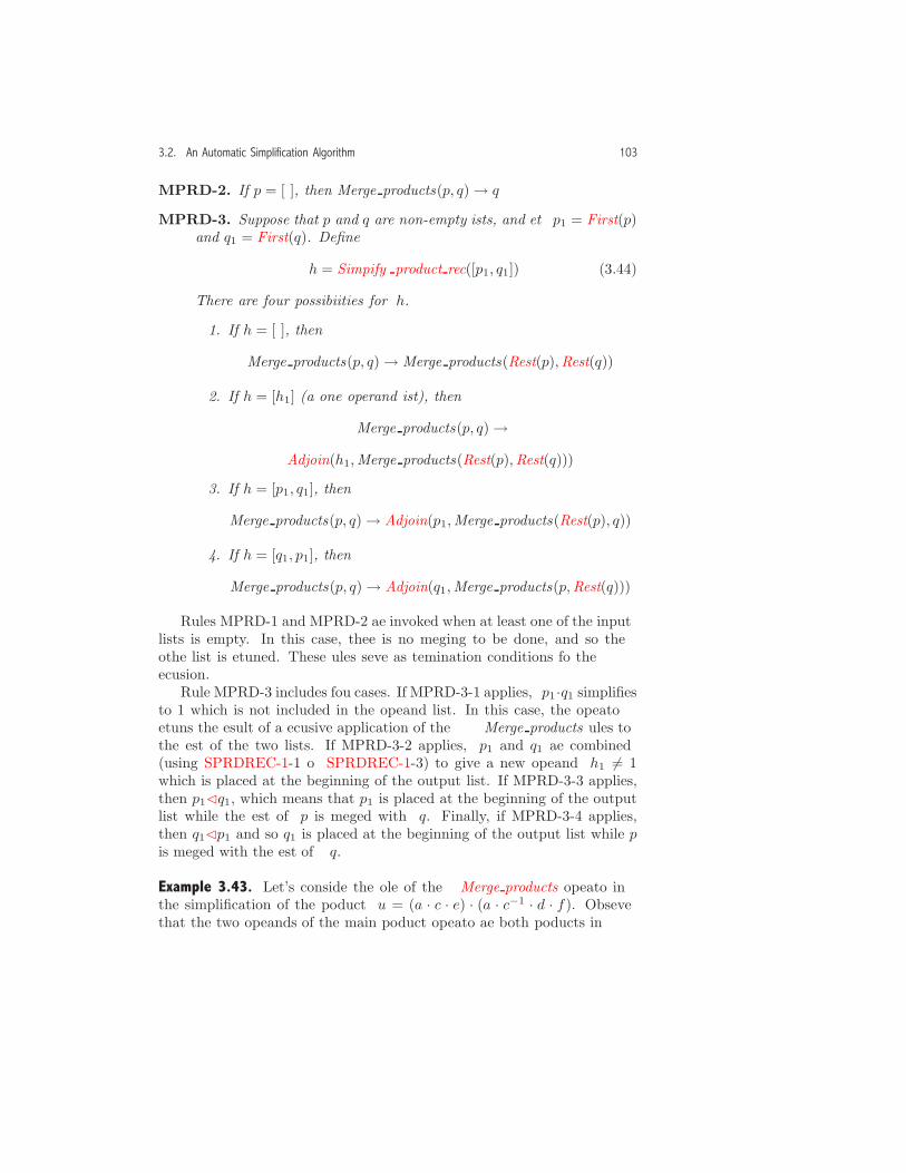
3.2. An Automatic Simplification Algorithm 103
MPRD-2. If p = [ ], then Merge products(p, q)→ q.
MPRD-3. Suppose that p and q are non-empty lists, and let p1 = First(p)and q1 = First(q). Define
h = Simplify product rec([p1, q1]). (3.44)
There are four possibilities for h.
1. If h = [ ], then
Merge products(p, q)→ Merge products(Rest(p),Rest(q)).
2. If h = [h1] (a one operand list), then
Merge products(p, q)→Adjoin(h1,Merge products(Rest(p),Rest(q))).
3. If h = [p1, q1], then
Merge products(p, q)→ Adjoin(p1,Merge products(Rest(p), q)).
4. If h = [q1, p1], then
Merge products(p, q)→ Adjoin(q1,Merge products(p,Rest(q))).
Rules MPRD-1 and MPRD-2 are invoked when at least one of the inputlists is empty. In this case, there is no merging to be done, and so theother list is returned. These rules serve as termination conditions for therecursion.
Rule MPRD-3 includes four cases. If MPRD-3-1 applies, p1 ·q1 simplifiesto 1 which is not included in the operand list. In this case, the operatorreturns the result of a recursive application of the Merge products rules tothe rest of the two lists. If MPRD-3-2 applies, p1 and q1 are combined(using SPRDREC-1-1 or SPRDREC-1-3) to give a new operand h1 �= 1which is placed at the beginning of the output list. If MPRD-3-3 applies,then p1✁q1, which means that p1 is placed at the beginning of the outputlist while the rest of p is merged with q. Finally, if MPRD-3-4 applies,then q1✁p1 and so q1 is placed at the beginning of the output list while pis merged with the rest of q.
Example 3.43. Let’s consider the role of the Merge products operator inthe simplification of the product u = (a · c · e) · (a · c−1 · d · f). Observethat the two operands of the main product operator are both products in
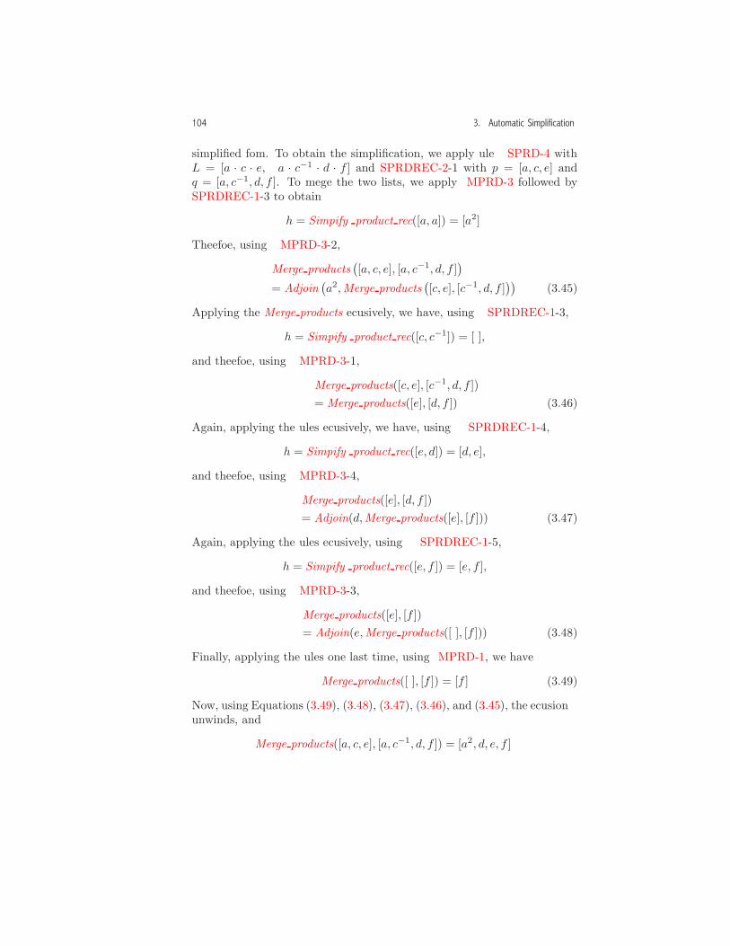
104 3. Automatic Simplification
simplified form. To obtain the simplification, we apply rule SPRD-4 withL = [a · c · e, a · c−1 · d · f ] and SPRDREC-2-1 with p = [a, c, e] andq = [a, c−1, d, f ]. To merge the two lists, we apply MPRD-3 followed bySPRDREC-1-3 to obtain
h = Simplify product rec([a, a]) = [a2].
Therefore, using MPRD-3-2,
Merge products([a, c, e], [a, c−1, d, f ]
)= Adjoin
(a2,Merge products
([c, e], [c−1, d, f ]
)). (3.45)
Applying the Merge products recursively, we have, using SPRDREC-1-3,
h = Simplify product rec([c, c−1]) = [ ],
and therefore, using MPRD-3-1,
Merge products([c, e], [c−1, d, f ])= Merge products([e], [d, f ]). (3.46)
Again, applying the rules recursively, we have, using SPRDREC-1-4,
h = Simplify product rec([e, d]) = [d, e],
and therefore, using MPRD-3-4,
Merge products([e], [d, f ])= Adjoin(d,Merge products([e], [f ])). (3.47)
Again, applying the rules recursively, using SPRDREC-1-5,
h = Simplify product rec([e, f ]) = [e, f ],
and therefore, using MPRD-3-3,
Merge products([e], [f ])= Adjoin(e,Merge products([ ], [f ])). (3.48)
Finally, applying the rules one last time, using MPRD-1, we have
Merge products([ ], [f ]) = [f ]. (3.49)
Now, using Equations (3.49), (3.48), (3.47), (3.46), and (3.45), the recursionunwinds, and
Merge products([a, c, e], [a, c−1, d, f ]) = [a2, d, e, f ].

3.2. An Automatic Simplification Algorithm 105
Therefore,
Simplify product rec([a · c · e, a · c−1 · d · f ])→ [a2, d, e, f ],
andSimplify product((a · c · e) · (a · c−1 · d · f))→ a2 · d · e · f. �
Simplification of Sums
The Simplify sum operator, which simplifies a sum to either an ASAE orthe symbol Undefined, is based on the following transformations:
1. the basic distributive transformation in Definition 3.1,
2. the basic associative transformation in Definition 3.5(1),
3. the basic commutative transformation for sums in Definition 3.7,
4. the basic identity transformation (3.20),
5. the basic unary transformation (3.33),
6. the basic numerical transformation in Definition 3.17(2), and
7. the basic “Undefined” transformation in Definition 3.18.
The operator is defined in terms of the following procedures.
1. The main procedure Simplify sum is defined by a sequence of non-recursive transformation rules. The rules are similar to those forSimplify product in Definition 3.37 although there is no analogue forrule SPRD-2.
2. The procedure Simplify sum rec is defined by recursive transforma-tion rules that are similar to the ones for Simplify product rec in Def-inition 3.38. In this case the analogue of SPRDREC-1-3 is based onthe basic distributive transformation in Definition 3.1.
3. The procedureMerge sums is defined by a sequence of recursive trans-formation rules that are similar to the ones for Merge products inDefinition 3.42.
We leave the details of the transformation rules and operators to the reader(Exercise 7).

106 3. Automatic Simplification
Simplification of Quotients, Differences, Factorials, andFunctions
The operator Simplify quotient, which simplifies quotients, is based on thebasic quotient transformation u/v = u · v−1. Observe that this transfor-mation creates a new power and a new product which are simplified usingthe Simplify power and Simplify product operators.
The operator Simplify difference(u) is based on the basic differencetransformations −u = (−1) · u and u − v = u + (−1) · v. Observe thatthese transformations create either a new product or a new sum which issimplified using either the Simplify product or Simplify sum operators.
The operator Simplify factorial(u) is based on the basic numerical trans-formation Definition 3.17(4) which evaluates a factorial with a non-negativeinteger operand. If the operand of a factorial isUndefined, then the proce-dure returnsUndefined. In other cases, the input expression u is returnedwithout change.
The operator Simplify function(u) applies to function forms. Althoughthere are no function transformations in our algorithm, some function argu-ment may be Undefined, in which case the operator returns Undefined.In other cases, return the input argument u without change.
The details of procedures for these operators are left to the reader (Ex-ercise 6).
Algebraic Properties of ASAEs
Consider the set of all ASAEs, and, for u and v in this set, define the sumof u and v as
Automatic simplify(u+ v)
and the product of u and v as
Automatic simplify(u · v).
This set together with these operations satisfies all the field axioms exceptthe distributive axioms F-7 and F-8 and the additive inverse axiom F-11.Axioms F-1, F-2, F-3, F-4, F-5, and F-6 follow directly from the trans-formation rules in this section. Axiom F-10 follows from SPRDREC-1-1and SPRDREC-1-2, and Axiom F-9 follows from similar rules for sums(Exercise 7). Axiom F-12 follows from SINTPOW-4 and SPRDREC-1-3.
On the other hand, the distributive axioms F-7 and F-8 are not alwaystrue because expansion is not included in automatic simplification. Forexample, for a, b, and c symbols, the expressions a ·(b+c) and a ·b+a ·c areboth already simplified but these expressions are not the same as expression
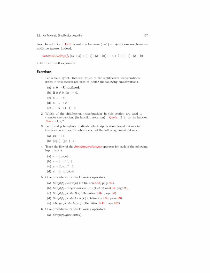
3.2. An Automatic Simplification Algorithm 107
trees. In addition, F-11 is not true because (−1) · (a+ b) does not have anadditive inverse. Indeed,
Automatic simplify((a+ b) + (−1) · (a+ b))→ a+ b+ (−1) · (a+ b)
rather than the 0 expression.
Exercises1. Let u be a symbol. Indicate which of the simplification transformations
listed in this section are used to perform the following transformations.
(a) u/0 → Undefined.
(b) If u �= 0, 0/u → 0.
(c) u/1 → u.
(d) u− 0 → 0.
(e) 0 − u → (−1) · u.
2. Which of the simplification transformations in this section are used totransform the quotient (in function notation) QuotOp(1, 2) to the fractionFracOp(1, 2)?
3. Let x and y be symbols. Indicate which simplification transformations inthis section are used to obtain each of the following transformations.
(a) x/x → 1.
(b) (x/y) · (y/x) → 1
4. Trace the flow of the Simplify product rec operator for each of the followinginput lists u.
(a) u = [c, b, a].
(b) u = [a, a−1, 1].
(c) u = [b, a, a−1, 1].
(d) u = [a, c, b, d, e].
5. Give procedures for the following operators.
(a) Simplify power(u) (Definition 3.33, page 94).
(b) Simplify integer power(v, n) (Definition 3.34, page 95).
(c) Simplify product(u) (Definition 3.37, page 98).
(d) Simplify product rec(L) (Definition 3.38, page 99).
(e) Merge products(p, q) (Definition 3.42, page 102).
6. Give procedures for the following operators.
(a) Simplify quotient(u).
108 3. Automatic Simplification
(b) Simplify difference(u).
(c) Simplify factorial(u).
(d) Simplify function(u).
(See the discussion starting on page 106.)
7. (a) Give transformation rules for the operators.
i. Simplify sum(u).
ii. Simplify sum rec(L).
iii. Merge sums(p, q).
(See the discussion starting on page 105.)
(b) Give procedures for these operators.
8. Modify the automatic simplification algorithm so that for a product withtwo operands, one a constant and the other a sum, the constant is dis-tributed over the sum. For example, the modification should obtain
Automatic simplify(2 · (x + y)) → 2 · x + 2 · y.If a product has more than two operands, the transformation does notoccur. For example, 2 · (3 + x) · (4 + x) is not changed. Hint: The bestplace to apply this transformation is in SPRD-4.
9. For ı =√−1, modify the automatic simplification algorithm so that all field
operations in Q(ı) (including integer powers and quotients) are performedby automatic simplification. (An algorithm for simplifying expressions withGaussian rational numbers is described in Exercise 19, page 61.)
10. Let N be a set of variables that are designated as integer variables. De-fine an integer expression as one constructed using the symbols in N , theintegers, and the addition, multiplication, and power (with non-negativeinteger exponents) operations.
(a) Let u be an ASAE. Give a procedure Integer expression(u) thatreturns true if u is an integer expression and false otherwise. Usefunction notation for u.
(b) Modify the automatic simplification algorithm so that the transfor-mations (3.15) and (3.16) are applied when n is an integer expression.
11. Let u be an ASAE in function notation and let x be a symbol. Give aprocedure Derivative fun(u, x) that obtains the derivative of u with respectto x. Be sure to return the derivative as an ASAE.
Further Reading
3.1 The Goal of Automatic Simplification. Discussions of automatic simpli-
fication are given in Fateman [36], Korsvold [57], Nievergelt, Farrar, and Reingold

3.2. An Automatic Simplification Algorithm 109
[75], Tobey, Bobrow, and Zilles [95], Weissman [99], Wooldridge [103], Wulf et
al. [104], and Yun and Stoutemyer [107]. Stoutemyer [94] gives an interesting
discussion of the misuse of some automatic simplification transformation rules.
Moses [71] has an interesting discussion of algebraic simplification.


4
Single Variable Polynomials
In this chapter we are concerned with the mathematical and computationalproperties of polynomials with one variable with coefficients from a field F.All the algorithms considered here are ultimately based on polynomialdivision.
In Section 4.1 we introduce the basic definitions, describe an algorithmfor polynomial division, and then give an algorithm for polynomial expan-sion. In Section 4.2 we examine the gcd problem for polynomials and giveversions of Euclid’s algorithm and the extended Euclidean algorithm in thissetting. In Section 4.3 we use the procedures in the first two sections toperform arithmetic operations for expressions in simple algebraic numberfields and to extend the polynomial operations to this setting. In Section4.4 we describe an algorithm for partial fraction expansion that is basedon polynomial division, polynomial expansion, and the extended Euclideanalgorithm.
Since the mathematical definitions and theorems apply for any coeffi-cient field F, we present the ideas in this general setting. In a computationalsetting, however, the algorithms make most sense for coefficient fields wherecomputation is effective and efficient.
4.1 Elementary Concepts and Polynomial Division
Let u be a polynomial of the form
u = unxn + un−1x
n−1 + · · ·+ u1x+ u0,
111

112 4. Single Variable Polynomials
where the coefficients uj are from a field F. The notation F[x] representsthe set of all such polynomials.
Recall that lc(u, x) represents the leading coefficient of a polynomialand deg(u, x) its degree.1 A polynomial with lc(u, x) = 1 is called a monicpolynomial.
The operators lc and deg satisfy the properties in the following theorem.
Theorem 4.1.Let u and v be polynomials in F[x].
1. lc(u v) = lc(u) lc(v).
2. If u �= 0 and v �= 0, then deg(u v) = deg(u) + deg(v).
3. deg(u± v) ≤ max({deg(u), deg(v)}).
Proof: To prove (1), first, when either u = 0 or v = 0, both sides of theequality are 0. Next, if both u �= 0 and v �= 0, the highest order monomialin u v is lc(u) lc(v)xdeg(u)+deg(v). Since both lc(u) and lc(v) are not zero,and since there are no zero divisors in a field (Theorem 2.36, page 50), theproduct lc(u) lc(v) �= 0, and so (1) follows.
The proof for Part (2) is similar to the proof for Part (1).Property (3) follows from the definition of degree. Notice that this re-
lationship is an inequality because addition (or subtraction) may eliminatethe leading terms of the polynomials. �
Theorem 4.2. Let u and v be polynomials in F[x]. If u v = 0, then eitheru = 0 or v = 0.
This theorem, which is a consequence of Theorem 4.1(1), states thatthere are no zero divisors in F[x]. The proof of the theorem is left to thereader (Exercise 3).
Polynomial Division
For single variable polynomials, the familiar process of long division of uby v is defined formally using recurrence relations.
1When the variable x is evident from context, we use the simpler notations lc(u) anddeg(u).

4.1. Elementary Concepts and Polynomial Division 113
Definition 4.3. Let u and v �= 0 be two polynomials in F[x], and considerthe sequence of quotients qi and remainders ri:
q0 = 0, r0 = u,
qi = qi−1 +lc(ri−1)lc(v)
xdeg(ri−1)−deg(v), (4.1)
ri = ri−1 − lc(ri−1)lc(v)
xdeg(ri−1)−deg(v) v. (4.2)
The iteration terminates when
deg(ri) < deg(v). (4.3)
If the process terminates with i = σ, then qσ is the quotient of u dividedby v, and rσ is the remainder. We also represent the quotient and theremainder by the operators quot(u, v, x) and rem(u, v, x).
Example 4.4. Let u = 5 x2 + 4 x+ 1 and v = 2 x+ 3. Then,
q0 = 0, r0 = 5 x2 + 4 x+ 1,q1 = 5/2 x, r1 = −7/2 x+ 1,q2 = 5/2 x− 7/4, r2 = 25/4.
Since deg(r2) < deg(v), the process stops after two iterations (σ = 2),and
u = qσ v + rσ = (5/2 x− 7/4) (2 x+ 3) + 25/4. �
Polynomial division satisfies the properties in the following theorem.
Theorem 4.5. Let u and v �= 0 be polynomials in F[x].
1. The polynomial division process terminates.
2. Let qσ and rσ be defined by the iteration in Definition 4.3. Then,
u = qσ v + rσ (4.4)
anddeg(rσ) < deg(v). (4.5)
3. The quotient qσ and the remainder rσ are unique in the sense thatthey are the only polynomials that satisfy both conditions (4.4) and (4.5).

114 4. Single Variable Polynomials
The property of the remainder in the inequality (4.5) is called the Eu-clidean property of polynomial division.
Proof: To show (1), let’s assume that we have obtained ri−1 (which doesnot satisfy the termination condition (4.3)), and show that
deg(ri) < deg(ri−1). (4.6)
This condition implies that the inequality (4.3) is eventually satisfied forsome ri.
Since the process does not terminate with ri−1, we have
deg(ri−1) ≥ deg(v). (4.7)
It is convenient to express the recurrence relation for ri in the form
ri =(ri−1 − lc(ri−1)x deg(ri−1)
)(4.8)
−(v − lc(v)x deg(v)
) (lc(ri−1)lc(v)
)x deg(ri−1)− deg(v)
which is equivalent to the form (4.2). There are two cases. First, if v is themonomial lc(v)x deg(v), then Equation (4.8) implies
deg(ri) = deg(ri−1 − lc(ri−1)x deg(ri−1)
)< deg(ri−1). (4.9)
On the other hand, when v−lc(v)x deg(v) �= 0, Equation (4.8) and Theorem4.1(2),(3) imply that
deg(ri) ≤ max({
deg(ri−1 − lc(ri−1)x deg(ri−1)
),
deg(x deg(ri−1)− deg(v)
(v − lc(v)x deg(v)
) )})≤ max
({deg
(ri−1 − lc(ri−1)x deg(ri−1)
),
( deg(ri−1)− deg(v)) + deg(v − lc(v)x deg(v)
)})< deg(ri−1).
Therefore, the inequality (4.6) is satisfied, and in this case, deg(rσ) <deg(v).To show (2), first observe that if deg(v) > deg(u), there are no iter-
ations (σ = 0), and Equation (4.4) is satisfied with qσ = 0 and rσ = u.If deg(v) ≤ deg(u), there is at least one iteration. From Equations (4.1)and (4.2), we have
qi v + ri = qi−1 v + ri−1, i = 1, 2, . . . , σ, (4.10)
and therefore

4.1. Elementary Concepts and Polynomial Division 115
u = q0 v + r0 = q1 v + r1 = · · · = qσ v + rσ.
The inequality (4.5) is satisfied because it is the stopping criterion for theiteration.
To verify the uniqueness property (3), suppose that there are two pairsof polynomials qσ1 , rσ1 and qσ2 , rσ2 that satisfy the conditions (4.4) and(4.5). Then,
u = qσ1 v + rσ1 = qσ2 v + rσ2 ,
and so(qσ1 − qσ2) v = rσ2 − rσ1 . (4.11)
First, if deg(v) = 0, then the inequality (4.5) implies rσ1 = rσ2 = 0, andso qσ1 = qσ2 as well. Suppose next that deg(v) > 0. If qσ1 − qσ2 �= 0, then
deg((qσ1 − qσ2) v) ≥ deg(v). (4.12)
However, (4.5) implies
deg(rσ2 − rσ1) < deg(v), (4.13)
and since the conditions (4.11), (4.12), and (4.13) cannot all be true, itmust be that qσ1 − qσ2 = 0, and so qσ1 = qσ2 and rσ1 = rσ2 . �
The approach that we used to prove the uniqueness property is called adegree argument because it is based primarily on the properties of degree.Degree arguments are frequently used to obtain properties of polynomials.
Theorem 4.6. Let u be a polynomial in F[x] with positive degree, andsuppose that c in F is a root of u = 0. Then, u can be factored as u =(x− c) q, where q is in F[x].
The proof of the theorem, which follows directly from Theorem 4.5, isleft to the reader (Exercise 13).
In Figure 4.1, we give a procedure for polynomial division and functionsthat extract the quotient and remainder.2 Observe that in line 10 we have
2When deg(v) = 0, the termination of Polynomial division at line 6 depends on
deg(0) → −∞. (4.14)
This operation is obtained by the MPL operator Degree gpe used at lines 3, 4, and 11. Ifa CAS’s degree operator is used instead, it must also obtain the operation (4.14). BothMaple’s degree operator and Mathematica’s Exponent operator obtain (4.14), whileMuPAD’s degree operator obtains deg(0) → 0. If the MuPAD implementation uses itsdegree operator, line 6 must be replaced by
while m ≥ n and r �= 0 do .

116 4. Single Variable Polynomials
Procedure Polynomial division(u, v, x);Input
u, v : GPEs in x with v �= 0;x : a symbol;
Outputa list [q, r] with quotient q and remainder r;
Local Variablesq, r,m,n, lcv, s, lcr;
Begin1 q := 0;2 r := u;3 m := Degree gpe(r, x)4 n := Degree gpe(v, x)5 lcv := Leading Coefficient gpe(v, x);6 while m ≥ n do7 lcr := Leading Coefficient gpe(r, x);8 s := lcr/lcv;9 q := q + s ∗ xm−n;10 r := Algebraic expand((r − lcr ∗ xm) − (v − lcv ∗ xn) ∗ s ∗ xm−n);11 m := Degree gpe(r, x);12 Return([q, r])
End
Quotient(u, v, x)function
:= Operand(Polynomial division(u, v, x), 1);
Remainder(u, v, x)function
:= Operand(Polynomial division(u, v, x), 2);
Figure 4.1. An MPL procedure for polynomial division of u by v in F[x]. (Im-plementation: Maple (txt), Mathematica (txt), MuPAD (txt).)
used the iteration formula for ri in Equation (4.8) rather than the formulain Equation (4.2). In fact, as long as all the field operations in F areobtained by automatic simplification, we can use Equation (4.2). However,when some field operations are not included in automatic simplification,Equation (4.2) may not eliminate the leading term from ri−1, and thealgorithm may not terminate. In Exercise 7, we give an example where theprocedure with line 10 replaced by the formula in Equation (4.2) does notterminate.
Although the Polynomial division procedure terminates whenever uand v are GPEs in x, for some coefficient fields it may return qσ and rσ

4.1. Elementary Concepts and Polynomial Division 117
in an inappropriate form. In Maple, Mathematica, and MuPAD, two fieldswhere it does give appropriate results areQ andQ(ı), because all numericalsimplifications (in lines 8 and 10) are handled by automatic simplification.For example, for the polynomials in Q(ı)[x]:
u = (2 + 4ı)x2 + (−1− 8ı)x+ (−3 + 3ı),
v = (1 + 2ı)x+ (1− ı),
all three systems obtain with two iterations qσ = 2 x− 3 and rσ = 0.On the other hand, consider the polynomials in Q(
√2)[x]:
u = (2− 4√2)x2 + (−1 + 4
√2)x+ (−3 + 3
√2),
v = (1− 2√2)x+ (1−
√2),
where u = (2 x − 3) v. In this case, all three systems obtain the involvedexpressions
qσ =2− 4
√2
1− 2√2x+−1 + 4
√2− 10
1−2√
2+ 6
√2
1−2√
2
1− 2√2
,
rσ = −3 + 3√2 +
91− 2
√2− 5
√2
1− 2√2+
22(1− 2
√2)2 − 16
√2(
1− 2√2)2 ,
rather than the simplified forms
qσ = 2 x− 3, rσ = 0.
The problem here is that some field operations for Q(√2) are not obtained
by automatic simplification in these systems. As we shall see in Section 4.2,this is more than just an inconvenience because the greatest common divisoralgorithm given in that section gives an incorrect result when it cannotdetermine that a remainder is zero.
Polynomial Divisors
Definition 4.7. Let u, v, and q be polynomials in F[x]. A polynomial v �= 0is a divisor of (or divides) a polynomial u if there is a polynomial q suchthat u = q v. We use the notation v | u to indicate that v is a divisor of uand v /| u if it does not. The polynomial q is called the cofactor of v in uand is represented by cof(v, u).
Example 4.8. For the polynomials in Q[x]:
u = x2 + 5x+ 6, v = x+ 2, (4.15)

118 4. Single Variable Polynomials
then v|u with q = cof(v, u) = x+ 3. In general, if v|u, then for c �= 0 in F,c v|u as well because
u = q v = ((1/c) q) (c v).
Therefore, 2 x+ 4 is also a divisor of u in (4.15). �
Definition 4.9. Let u, v, and w be polynomials in F[x].
1. A common divisor (or common factor) of u and v is a polynomialw such that w|u and w|v.
2. The polynomials u and v are relatively prime if they have no com-mon divisor of positive degree.
Example 4.10. The polynomial x + 2 is a common divisor of u = x2 − 4and v = x2 + 5x + 6. The polynomials x2 − 4 and x2 − 1 are relativelyprime. �
Irreducible Polynomials
An irreducible polynomial is the polynomial analogue of a prime number.
Definition 4.11. A polynomial u in F[x] is reducible if there are polyno-mials v and w in F[x] with positive degree such that u = v w. A polynomialis irreducible if it is not reducible.
Irreducibility depends, of course, on the coefficient field.
Example 4.12. The polynomial x2 − 2 is irreducible when F = Q but isreducible as x2 − 2 = (x−√2)(x +√2) when F = Q(
√2). �
Polynomial Expansion
The polynomial expansion of u in terms of v involves the representationof u as a sum whose terms contain non-negative integer powers of v. Thefollowing polynomial expansion theorem is based on polynomial division.
Theorem 4.13. Let u and v be polynomials in F[x], and suppose that v haspositive degree. Then, there are unique polynomials
dk(x), dk−1(x), . . . , d0(x)

4.1. Elementary Concepts and Polynomial Division 119
with deg(di) < deg(v) such that
u = dkvk + dk−1v
k−1 + · · ·+ d1v + d0. (4.16)
The representation for u in Equation (4.16) is called the polynomialexpansion3 of u in terms of v. For example, for
u = x5 + 11x4 + 51x3 + 124x2 + 159x+ 86, v = x2 + 4x+ 5,
thenu = (x + 3) v2 + (x+ 2) v + (x+ 1).
When v = x − c, the polynomial expansion coincides with the Taylor ex-pansion of u about x = c (Exercise 15).
Proof of Theorem 4.13: We show first that the sequence d0, d1, . . . , dk existsby giving an algorithm to compute it. Using polynomial division, there arepolynomials c0 and d0 such that
u = c0 v + d0, (4.17)
where deg(d0) < deg(v). If c0 = 0, there is only one term in the expansion(k = 0) with u = d0. If c0 �= 0 but deg(c0) < deg(v), then the expansionhas two terms (k = 1) with d1 = c0 and d0 defined by Equation (4.17).Finally, if deg(c0) ≥ deg(v), form the quotient sequence
u = c0 v + d0,
c0 = c1 v + d1,
c1 = c2 v + d2,
... (4.18)ck−2 = ck−1 v + dk−1,
ck−1 = ck v + dk,
ck = 0,
where ci = quot(ci−1, v, x), di = rem(ci−1, v, x), and deg(di) < deg(v).Since Theorem 4.1 implies deg(ci) < deg(ci−1), the quotient sequenceterminates after a finite number of steps with ck = 0. Substituting theexpression for ci into the expression for ci−1, we obtain
3Don’t confuse polynomial expansion with the Algebraic expand operation, whichactually destroys a polynomial expansion. The term expansion is used here as it is inthe Taylor expansion of a function in calculus.
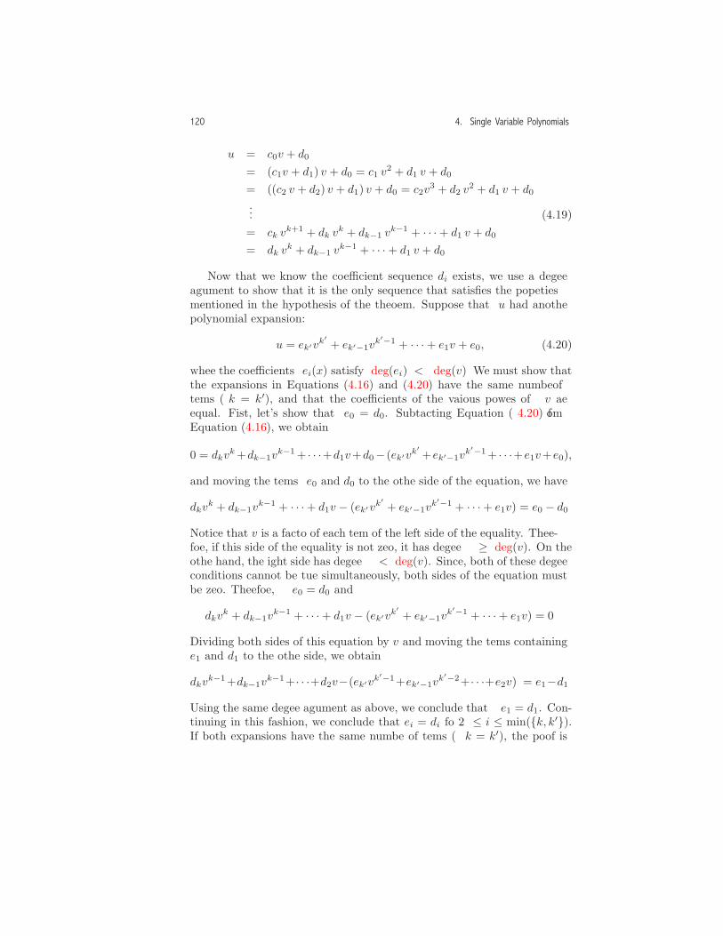
120 4. Single Variable Polynomials
u = c0v + d0
= (c1v + d1) v + d0 = c1 v2 + d1 v + d0
= ((c2 v + d2) v + d1) v + d0 = c2v3 + d2 v
2 + d1 v + d0
... (4.19)= ck v
k+1 + dk vk + dk−1 v
k−1 + · · ·+ d1 v + d0
= dk vk + dk−1 v
k−1 + · · ·+ d1 v + d0.
Now that we know the coefficient sequence di exists, we use a degreeargument to show that it is the only sequence that satisfies the propertiesmentioned in the hypothesis of the theorem. Suppose that u had anotherpolynomial expansion:
u = ek′vk′ + ek′−1v
k′−1 + · · ·+ e1v + e0, (4.20)
where the coefficients ei(x) satisfy deg(ei) < deg(v). We must show thatthe expansions in Equations (4.16) and (4.20) have the same number ofterms (k = k′), and that the coefficients of the various powers of v areequal. First, let’s show that e0 = d0. Subtracting Equation (4.20) fromEquation (4.16), we obtain
0 = dkvk+dk−1v
k−1+ · · ·+d1v+d0− (ek′vk′ +ek′−1vk′−1+ · · ·+e1v+e0),
and moving the terms e0 and d0 to the other side of the equation, we have
dkvk + dk−1v
k−1 + · · ·+ d1v − (ek′vk′+ ek′−1v
k′−1 + · · ·+ e1v) = e0 − d0.
Notice that v is a factor of each term of the left side of the equality. There-fore, if this side of the equality is not zero, it has degree ≥ deg(v). On theother hand, the right side has degree < deg(v). Since, both of these degreeconditions cannot be true simultaneously, both sides of the equation mustbe zero. Therefore, e0 = d0 and
dkvk + dk−1v
k−1 + · · ·+ d1v − (ek′vk′+ ek′−1v
k′−1 + · · ·+ e1v) = 0.
Dividing both sides of this equation by v and moving the terms containinge1 and d1 to the other side, we obtain
dkvk−1+dk−1v
k−1+· · ·+d2v−(ek′vk′−1+ek′−1vk′−2+· · ·+e2v) = e1−d1.
Using the same degree argument as above, we conclude that e1 = d1. Con-tinuing in this fashion, we conclude that ei = di for 2 ≤ i ≤ min({k, k′}).If both expansions have the same number of terms (k = k′), the proof is
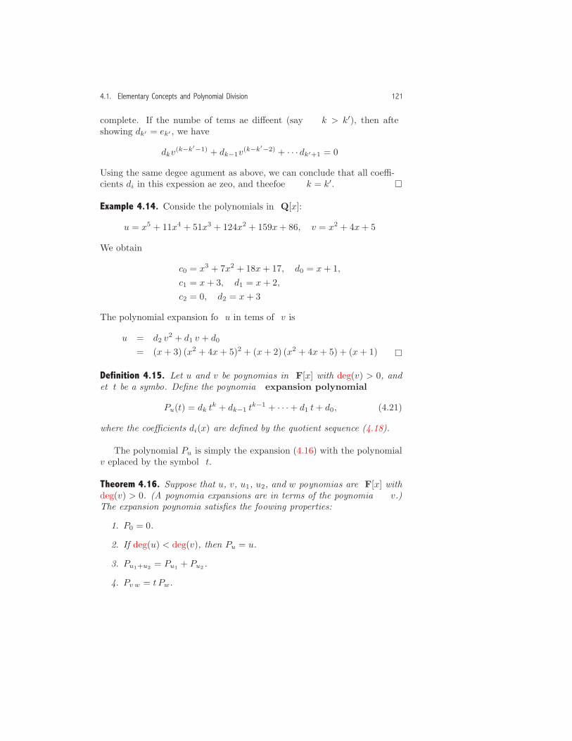
4.1. Elementary Concepts and Polynomial Division 121
complete. If the number of terms are different (say k > k′), then aftershowing dk′ = ek′ , we have
dkv(k−k′−1) + dk−1v
(k−k′−2) + · · · dk′+1 = 0.
Using the same degree argument as above, we can conclude that all coeffi-cients di in this expression are zero, and therefore k = k′. �
Example 4.14. Consider the polynomials in Q[x]:
u = x5 + 11x4 + 51x3 + 124x2 + 159x+ 86, v = x2 + 4x+ 5.
We obtain
c0 = x3 + 7x2 + 18x+ 17, d0 = x+ 1,c1 = x+ 3, d1 = x+ 2,c2 = 0, d2 = x+ 3.
The polynomial expansion for u in terms of v is
u = d2 v2 + d1 v + d0
= (x+ 3) (x2 + 4x+ 5)2 + (x+ 2) (x2 + 4x+ 5) + (x+ 1). �
Definition 4.15. Let u and v be polynomials in F[x] with deg(v) > 0, andlet t be a symbol. Define the polynomial expansion polynomial
Pu(t) = dk tk + dk−1 t
k−1 + · · ·+ d1 t+ d0, (4.21)
where the coefficients di(x) are defined by the quotient sequence (4.18).
The polynomial Pu is simply the expansion (4.16) with the polynomialv replaced by the symbol t.
Theorem 4.16. Suppose that u, v, u1, u2, and w polynomials are F[x] withdeg(v) > 0. (All polynomial expansions are in terms of the polynomial v.)The expansion polynomial satisfies the following properties:
1. P0 = 0.
2. If deg(u) < deg(v), then Pu = u.
3. Pu1+u2 = Pu1 + Pu2 .
4. Pv w = t Pw.

122 4. Single Variable Polynomials
Procedure Polynomial expansion(u, v, x, t);Input
u : a GPE in x;v : a GPE in x with deg(v, x) > 0 ;x, t : symbols;
OutputThe polynomial Pu;
Local Variablesd, q, r;
Begin1 if u = 0 then2 Return(0)3 else4 d := Polynomial division(u, v, x);5 q := Operand(d, 1);6 r := Operand(d, 2);7 Return(Algebraic expand( t ∗ Polynomial expansion(q, v, x, t) + r))
End
Figure 4.2. An MPL procedure for polynomial expansion. (Implementation:Maple (txt), Mathematica (txt), MuPAD (txt).)
The verification of these properties is straightforward and is left to thereader (Exercise 18).
The next theorem describes a recurrence relation that gives a simplealgorithm for computing Pu.
Theorem 4.17. Let u and v be polynomials in F[x] with deg(v, x) > 0, andsuppose that from polynomial division, u = q v + r. Then, the expansionpolynomial satisfies the recurrence relation
Pu = t Pq + r.
The proof follows directly from the previous theorem (Exercise 19).A recursive procedure to compute Pu is given in Figure 4.2. The pro-
cedure uses the condition in Theorem 4.16(1) for termination (lines 1–2).The Algebraic expand operator is applied to the recurrence relation (line 7)so that the expression is returned as a polynomial in t rather than as acomposite expression.
Notice that the procedure accepts u and v that are GPEs in x, al-though in some cases more simplification is required to obtain the ex-

4.1. Elementary Concepts and Polynomial Division 123
pansion in a usable form (Exercise 14(b)). Since deg(v) > 0, it followsthat deg(q) < deg(u), which implies that each successive recursive call in-volves a polynomial u of smaller degree. Therefore, for some recursive calldeg(u) < deg(v), which implies q = 0 at line 5, and the next call terminatesthe recursion.
To get the representation for u in Equation (4.16), evaluate the expres-sion
Substitute(Polynomial expansion(u, v, x, t), t = v). (4.22)
Example 4.18. For the polynomials in Example 4.14
u = x5 + 11 x4 + 51 x3 + 124 x2 + 159 x+ 86, v = x2 + 4 x+ 5,
and so
Polynomial expansion(u, v, x, t)→ x t2 + 3 t2 + x t+ 2 t+ x+ 1.
Applying the operation (4.22), we have the expansion
(x + 3) (x2 + 4 x+ 5)2 + (x + 2) (x2 + 4 x+ 5) + x+ 1. �
Expansion-Based Substitutions. Using polynomial expansion, we can gener-alize the notion of substitution for expressions in F[x] to allow substitutionsfor “hidden” polynomials. For example, let
u = (x+ 1)3 + 2 (x+ 1) + 4,
which has the algebraically expanded form
u = x3 + 3x2 + 5x+ 7. (4.23)
Now suppose that we would like to substitute t for x+1 in the polynomial(4.23). In this form, x + 1 is not a complete sub-expression of u, and sothe substitution is not possible with the structural substitution. However,the substitution is readily obtained with the operation
Polynomial expansion(u, x+ 1, x, t)→ t3 + 2 t+ 4.
In this sense, polynomial expansion is a generalization of substitution.
Expansion-Based Polynomial Operators. By using polynomial expansion,we can extend the polynomial structural operations (Degree gpe,Coefficient gpe, etc.) to polynomials u that are not (comfortably) poly-nomials in v in the sense of the definitions in Section 1.4. For example,although
u = 3 x4 + 5 x2 + 7
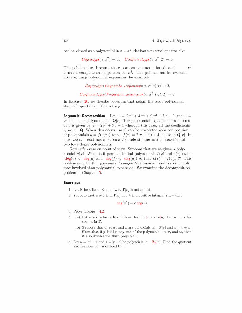
124 4. Single Variable Polynomials
can be viewed as a polynomial in v = x2, the basic structural operators give
Degree gpe(u, x2)→ 1, Coefficient gpe(u, x2, 2)→ 0.
The problem arises because these operators are structure-based, and x2
is not a complete sub-expression of x4. The problem can be overcome,however, using polynomial expansion. For example,
Degree gpe(Polynomial expansion(u, x2, t), t)→ 2,
Coefficient gpe(Polynomial expansion(u, x2, t), t, 2)→ 3.
In Exercise 20, we describe procedures that perform the basic polynomialstructural operations in this setting.
Polynomial Decomposition. Let u = 2 x4 + 4 x3 + 9 x2 + 7 x + 9 and v =x2+x+1 be polynomials in Q[x]. The polynomial expansion of u in termsof v is given by u = 2 v2 + 3 v + 4 where, in this case, all the coefficientsri are in Q. When this occurs, u(x) can be represented as a compositionof polynomials u = f(v(x)) where f(x) = 2 x2 + 3 x+ 4 is also in Q[x]. Inother words, u(x) has a particularly simple structure as a composition oftwo lower degree polynomials.
Now let’s reverse our point of view. Suppose that we are given a poly-nomial u(x). When is it possible to find polynomials f(x) and v(x) (withdeg(v) < deg(u) and deg(f) < deg(u)) so that u(x) = f(v(x))? Thisproblem is called the polynomial decomposition problem and is considerablymore involved than polynomial expansion. We examine the decompositionproblem in Chapter 5.
Exercises1. Let F be a field. Explain why F[x] is not a field.
2. Suppose that u �= 0 is in F[x] and k is a positive integer. Show that
deg(uk) = k deg(u).
3. Prove Theorem 4.2.
4. (a) Let u and v be in F[x]. Show that if u|v and v|u, then u = c v forsome c in F.
(b) Suppose that u, v, w, and p are polynomials in F[x] and u = v + w.Show that if p divides any two of the polynomials u, v, and w, thenit also divides the third polynomial.
5. Let u = x2 + 1 and v = x + 2 be polynomials in Z5[x]. Find the quotientand remainder of u divided by v.
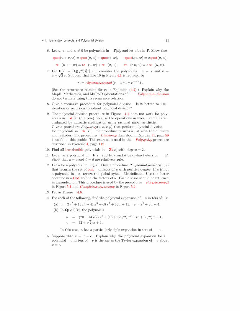
4.1. Elementary Concepts and Polynomial Division 125
6. Let u, v, and w �= 0 be polynomials in F[x], and let c be in F. Show that
quot(u + v,w) = quot(u,w) + quot(v,w), quot(c u,w) = c quot(u,w),
rem(u + v,w) = rem(u,w) + rem(v,w), rem(c u,w) = c rem(u,w).
7. Let F[x] = (Q(√
2))[x] and consider the polynomials u = x and v =x +
√2x. Suppose that line 10 in Figure 4.1 is replaced by
r := Algebraic expand r − v ∗ s ∗ xm−n .
(See the recurrence relation for ri in Equation (4.2).) Explain why theMaple, Mathematica, and MuPAD implementations of Polynomial divisiondo not terminate using this recurrence relation.
8. Give a recursive procedure for polynomial division. Is it better to useiteration or recursion to implement polynomial division?
9. The polynomial division procedure in Figure 4.1 does not work for poly-nomials in Zp[x] (p a prime) because the operations in lines 8 and 10 areevaluated by automatic simplification using rational number arithmetic.Give a procedure Poly div p(u, v, x, p) that performs polynomial divisionfor polynomials in Zp[x]. The procedure returns a list with the quotientand remainder. The procedure Division p described in Exercise 11, page 59is useful in this problem. This exercise is used in the Poly gcd p proceduredescribed in Exercise 4, page 142.
10. Find all irrreducible polynomials in Z3[x] with degree = 2.
11. Let h be a polynomial in F[x], and let c and d be distinct members of F.Show that h− c and h− d are relatively prime.
12. Let u be a polynomial in Q[x]. Give a procedure Polynomial divisors(u, x)that returns the set of monic divisors of u with positive degree. If u is nota polynomial in x, return the global symbol Undefined. Use the factoroperator in a CAS to find the factors of u. Each divisor should be returnedin expanded form. This procedure is used by the procedures Poly decomp 2in Figure 5.1 and Complete poly decomp in Figure 5.2.
13. Prove Theorem 4.6.
14. For each of the following, find the polynomial expansion of u in terms of v.
(a) u = 2 x5 + 13x4 + 41 x3 + 68x2 + 63 x + 11, v = x2 + 3x + 4.
(b) In Q(√
2)[x], the polynomials
u = (20 + 14√
2)x3 + (18 + 12√
2) x2 + (6 + 3√
2) x + 1,
v = (2 +√
2)x + 1.
In this case, u has a particularly simple expansion in terms of v.
15. Suppose that v = x − c. Explain why the polynomial expansion for apolynomial u in terms of v is the same as the Taylor expansion of u aboutx = c.

126 4. Single Variable Polynomials
16. Find the polynomial expansion of u = xn in terms of v = x − 1 for n =1, 2, 3, 4, 5. What pattern do you observe with the coefficients di? Explainwhy the coefficient pattern appears in these expansions.
17. Suppose that u is expressed as a polynomial expansion in terms of v withdeg(v) > 0. Show that deg(u) = deg(dk) + deg(v) k.
18. Prove Theorem 4.16.
19. Prove Theorem 4.17.
20. Let u and v be polynomials in Q[x] with deg(v, x) ≥ 1. Let’s define u tobe a polynomial in v if the coefficients di in the polynomial expansion ofu in terms of v are all rational numbers. For example, 3 x4 + 4x2 + 5 is apolynomial in terms of x2, while x3 + x2 is not. Give procedures for thefollowing operators.
(a) Polynomial exp(u, v, x) which returns true if u is a polynomial interms of v as defined above and false otherwise.
(b) Degree exp(u, v, x) which returns the degree of u in terms of v whenu is a polynomial in v or the symbol Undefined when u is not apolynomial in v.
(c) Coefficient exp(u, v, x, i) which returns the coefficient di when u is apolynomial in v or the symbol Undefined when u is not a polynomialin v.
4.2 Greatest Common Divisors in F[x]
The concept of the greatest common divisor of two polynomials u and vis a fundamental one in computer algebra. Loosely speaking, a greatestcommon divisor of u and v is a divisor of u and v that contains all thefactors that u and v have in common. The concept is defined formally inthe following definition.
Definition 4.19. Let u and v be polynomials in F[x]. The greatest com-mon divisor (gcd) of u and v (at least one of which is non-zero) is apolynomial d that satisfies the following properties.
1. d is a common divisor of u and v.
2. If e is any common divisor of u and v, then e|d.3. d is a monic polynomial.
The operator gcd(u, v, x) denotes the greatest common divisor. When thereis no chance of confusion, we omit the variable x and use the simplernotation gcd(u, v).
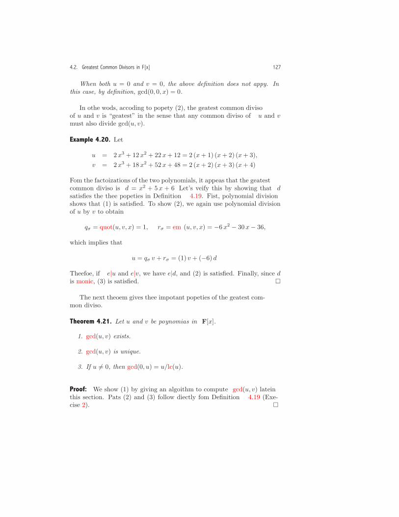
4.2. Greatest Common Divisors in F[x] 127
When both u = 0 and v = 0, the above definition does not apply. Inthis case, by definition, gcd(0, 0, x) = 0.
In other words, according to property (2), the greatest common divisorof u and v is “greatest” in the sense that any common divisor of u and vmust also divide gcd(u, v).
Example 4.20. Let
u = 2 x3 + 12 x2 + 22 x+ 12 = 2 (x+ 1) (x+ 2) (x+ 3),v = 2 x3 + 18 x2 + 52 x+ 48 = 2 (x+ 2) (x+ 3) (x+ 4).
From the factorizations of the two polynomials, it appears that the greatestcommon divisor is d = x2 + 5 x + 6. Let’s verify this by showing that dsatisfies the three properties in Definition 4.19. First, polynomial divisionshows that (1) is satisfied. To show (2), we again use polynomial divisionof u by v to obtain
qσ = quot(u, v, x) = 1, rσ = rem(u, v, x) = −6 x2 − 30 x− 36,
which implies that
u = qσ v + rσ = (1) v + (−6) d.
Therefore, if e|u and e|v, we have e|d, and (2) is satisfied. Finally, since dis monic, (3) is satisfied. �
The next theorem gives three important properties of the greatest com-mon divisor.
Theorem 4.21. Let u and v be polynomials in F[x].
1. gcd(u, v) exists.
2. gcd(u, v) is unique.
3. If u �= 0, then gcd(0, u) = u/lc(u).
Proof: We show (1) by giving an algorithm to compute gcd(u, v) later inthis section. Parts (2) and (3) follow directly from Definition 4.19 (Exer-cise 2). �

128 4. Single Variable Polynomials
Euclid’s GCD Algorithm in F[x]The gcd of two polynomials is obtained with a polynomial version of Eu-clid’s algorithm described in Section 2.1 The algorithm is based on thefollowing theorem.
Theorem 4.22. Let u and v �= 0 be polynomials in F[x], and let
rσ = rem(u, v, x).
Then,gcd(u, v) = gcd(v, rσ).
Proof: The proof of this theorem is the same as the proof for the integercase (see Theorem 2.9, page 21). �
We can find the gcd(u, v) by repeatedly applying Theorem 4.22. Whenv �= 0, define a sequence of polynomials R−1, R0, R1, . . . with the followingscheme:
R−1 = u,
R0 = v,
R1 = rem(R−1, R0, x),... (4.24)
Ri+1 = rem(Ri−1, Ri, x),...
The sequence (4.24) is called a polynomial remainder sequence. Since
deg(Ri+1) < deg(Ri),
some member of the sequence is 0. Let Rρ be the first such remainder. ByTheorem 4.22 and Theorem 4.21(3),
gcd(u, v) = gcd(R−1, R0)= gcd(R0, R1)... (4.25)= gcd(Rρ−1, Rρ−2)= gcd(Rρ−1, Rρ)= gcd(Rρ−1, 0)= Rρ−1/lc(Rρ−1),

4.2. Greatest Common Divisors in F[x] 129
where we have used the condition Rρ = 0 to terminate the iteration. Thisdiscussion is summarized in the following theorem.
Theorem 4.23. Let u and v be polynomials in F[x], at least one of whichis not zero. Then, gcd(u, v) = Rρ−1/lc(Rρ−1).
Proof: Although the relation was derived by assuming that v �= 0, it istrue when u �= 0 and v = 0 as well. In this case, ρ = 0 and gcd(u, 0) =u/lc(u) = R−1/lc(R−1). �
Example 4.24. Let u = x7−4 x5−x2+4 and v = x5−4 x3−x2+4. Then,
R1 = x4 − 5 x2 + 4, R2 = x3 − x2 − 4 x+ 4, R3 = 0.
Therefore, gcd(u, v) = x3 − x2 − 4 x+ 4. �
A procedure that obtains gcd(u, v) using the polynomial remainder se-quence (4.24) is given in Figure 4.3. Lines 1 and 2 are included so that adivision by zero is not encountered at line 6 for the special case when bothu = 0 and v = 0. The Algebraic expand operator at line 9 is included todistribute 1/Leading Coefficient gpe(U, x) when U is a sum.
Notice that in Polynomial gcd, we require that all field operations in Fbe obtained with automatic simplification. If this is not so, the proceduremay return an incorrect result. The next example illustrates this point.
Example 4.25. Consider the polynomials in Q(√
2)[x]:
u = x2 +(−1−
√2)x, v = x2 +
(−2− 2
√2)x+ 3 + 2
√2.
In this case, gcd(u, v) = x + (−1−√2). However, if automatic simplifica-tion does not perform all operations in Q(
√2)[x], we obtain the remainder
sequence4
R1 = x+√2x− 3− 2
√2,
R2 = 3+ 2√2− 14√
2 + 1− 10
√2√
2 + 1+
17(√2 + 1
)2 +12√2(√
2 + 1)2 ,
R3 = 0.
Since R2 is free of x, Polynomial gcd returns gcd(u, v) = 1, which is incor-rect. In fact, R2 simplifies to 0, and so the iteration should have terminatedwith R2 = 0, giving gcd(u, v) = R1/lc(R1) = x+ (−1−√2). �
4Similar results are obtained with Maple, Mathematica, and MuPAD implementa-tions of Polynomial division and Polynomial gcd.
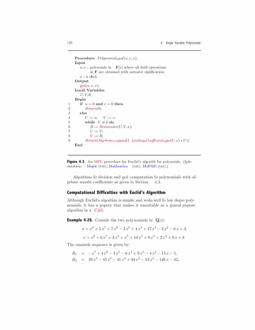
130 4. Single Variable Polynomials
Procedure Polynomial gcd(u, v, x);Input
u, v : polynomials in F[x] where all field operationsin F are obtained with automatic simplification;
x : a symbol;Output
gcd(u, v, x);Local VariablesU,V,R;
Begin1 if u = 0 and v = 0 then2 Return(0)3 else4 U := u; V := v;5 while V �= 0 do6 R := Remainder(U, V, x);7 U := V ;8 V := R;9 Return(Algebraic expand(1/Leading Coefficient gpe(U, x) ∗ U))
End
Figure 4.3. An MPL procedure for Euclid’s algorithm for polynomials. (Imple-mentation: Maple (txt), Mathematica (txt), MuPAD (txt).)
Algorithms for division and gcd computation for polynomials with al-gebraic number coefficients are given in Section 4.3.
Computational Difficulties with Euclid’s Algorithm
Although Euclid’s algorithm is simple and works well for low degree poly-nomials, it has a property that makes it unsuitable as a general purposealgorithm in a CAS.
Example 4.26. Consider the two polynomials in Q[x]:
u = x8 + 5 x7 + 7 x6 − 3 x5 + 4 x4 + 17 x3 − 2 x2 − 6 x+ 3,
v = x8 + 6 x7 + 3 x6 + x5 + 10 x4 + 8 x3 + 2 x2 + 9 x+ 8.
The remainder sequence is given by:
R1 = −x7 + 4 x6 − 4 x5 − 6 x4 + 9 x3 − 4 x2 − 15 x− 5,R2 = 39 x6 − 45 x5 − 41 x4 + 94 x3 − 53 x2 − 146 x− 42,
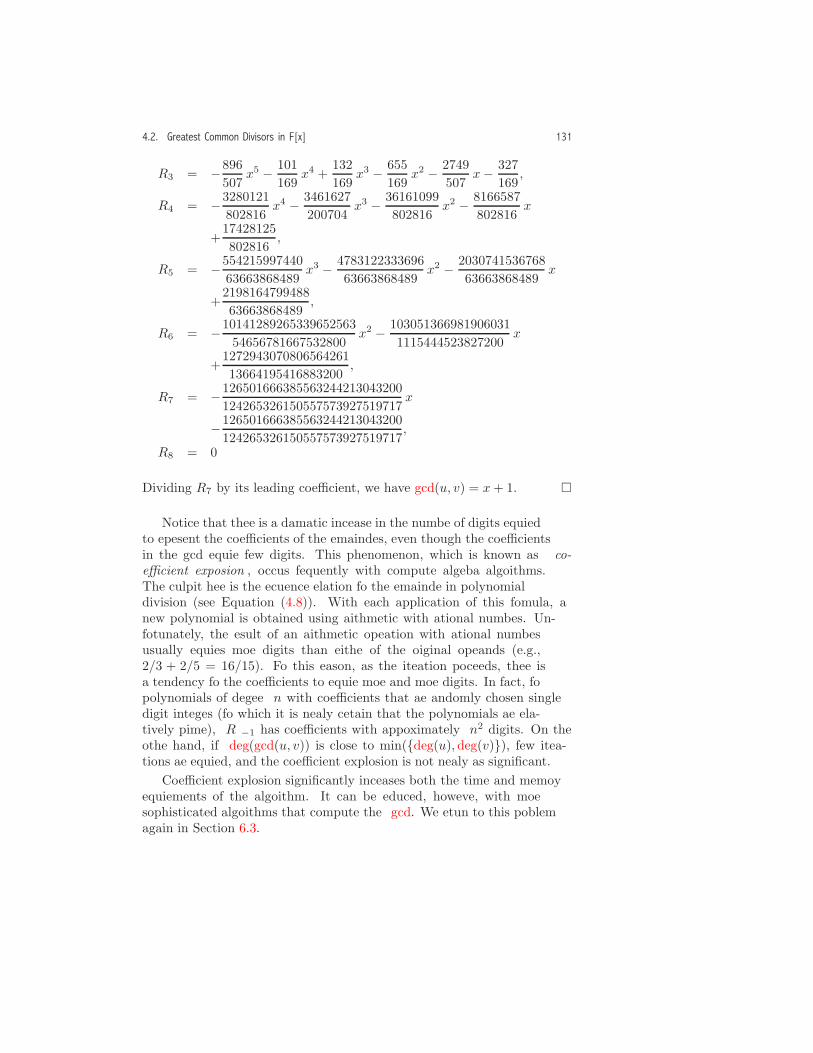
4.2. Greatest Common Divisors in F[x] 131
R3 = −896507
x5 − 101169
x4 +132169
x3 − 655169
x2 − 2749507
x− 327169
,
R4 = −3280121802816
x4 − 3461627200704
x3 − 36161099802816
x2 − 8166587802816
x
+17428125802816
,
R5 = −55421599744063663868489
x3 − 478312233369663663868489
x2 − 203074153676863663868489
x
+219816479948863663868489
,
R6 = −1014128926533965256354656781667532800
x2 − 1030513669819060311115444523827200
x
+127294307080656426113664195416883200
,
R7 = −126501666385563244213043200124265326150557573927519717
x
−126501666385563244213043200124265326150557573927519717
,
R8 = 0.
Dividing R7 by its leading coefficient, we have gcd(u, v) = x+ 1. �
Notice that there is a dramatic increase in the number of digits requiredto represent the coefficients of the remainders, even though the coefficientsin the gcd require few digits. This phenomenon, which is known as co-efficient explosion, occurs frequently with computer algebra algorithms.The culprit here is the recurrence relation for the remainder in polynomialdivision (see Equation (4.8)). With each application of this formula, anew polynomial is obtained using arithmetic with rational numbers. Un-fortunately, the result of an arithmetic operation with rational numbersusually requires more digits than either of the original operands (e.g.,2/3 + 2/5 = 16/15). For this reason, as the iteration proceeds, there isa tendency for the coefficients to require more and more digits. In fact, forpolynomials of degree n with coefficients that are randomly chosen singledigit integers (for which it is nearly certain that the polynomials are rela-tively prime), Rρ−1 has coefficients with approximately n2 digits. On theother hand, if deg(gcd(u, v)) is close to min({deg(u), deg(v)}), few itera-tions are required, and the coefficient explosion is not nearly as significant.
Coefficient explosion significantly increases both the time and memoryrequirements of the algorithm. It can be reduced, however, with moresophisticated algorithms that compute the gcd. We return to this problemagain in Section 6.3.

132 4. Single Variable Polynomials
The Extended Euclidean Algorithm in F[x]An extended Euclidean algorithm for polynomials in F[x] is similar to thealgorithm for the integers described in Section 2.1.
Theorem 4.27. For u and v polynomials in F[x], there exist polynomials Aand B in F[x] such that
Au+B v = gcd(u, v). (4.26)
The polynomials A and B are given in Equation (4.31).
Proof: Since the development for polynomials is nearly identical to whatwas done for the integers (page 23), we only summarize the approach. First,for the special case u = 0 and v = 0, we use A = 0 and B = 0. Wheneither u or v is not zero, there are polynomials Ai and Bi such that
Ri = Ai u+Bi v. (4.27)
These polynomials are given by the recurrence relations:
A−1 = 1, A0 = 0, (4.28)
B−1 = 0, B0 = 1, (4.29)
Ai = Ai−2 −QiAi−1, Bi = Bi−2 −QiBi−1, i ≥ 1, (4.30)
where Qi = quot(Ri−2, Ri−1, x). Now, since gcd(u, v) = Rρ−1/lc(Rρ−1),we have
A = Aρ−1/lc(Rρ−1), B = Bρ−1/lc(Rρ−1). (4.31)
�
Example 4.28. Let
u = x7 − 4 x5 − x2 + 4, v = x5 − 4 x3 − x2 + 4.
The greatest common divisor of these polynomials is given in Example 4.24as gcd(u, v) = R2 = x3 − x2 − 4 x+ 4. In addition,
A1 = 1, B1 = −x2,
A2 = −x, B2 = x3 + 1.A3 = x2 + x+ 1, B3 = −x4 − x3 − x2 − x− 1.
Therefore, by Equation (4.31),
A = A2/lc(R2) = −x,
4.2. Greatest Common Divisors in F[x] 133
B = B2/lc(R2) = x3 + 1. �
A procedure that obtains A and B using the recurrence relations (4.30)with initial conditions (4.28) and (4.29) is given in Figure 4.4. The variablesAp and Bp represent the previous values Ai−1 and Bi−1, and App and Bpprepresent Ai−2 and Bi−2.
Theorem 4.27 has many applications in computer algebra including thestatements in the next theorem which are used frequently in the remainderof the book.
Theorem 4.29. Suppose that u, v, and w are in F[x].
1. If w|u v and w and u are relatively prime, then w|v.2. If w|u v and w is irrreducible, then w|u or w|v.3. If u|w, v|w, and gcd(u, v) = 1, then u v|w.
Proof: The proofs are similar to the ones for Theorem 2.16 on page 27.�
Using Theorem 4.27, we obtain the following description of relativelyprime polynomials.
Theorem 4.30. Let u and v be polynomials in F[x] at least one of which isnot 0. Then u and v are relatively prime if and only if there are polynomialsA and B in F[x] such that
Au+B v = 1. (4.32)
Proof: First, if u and v are relatively prime, then Theorem 4.27 impliesEquation (4.32).
On the other hand, if Equation (4.32) is true, then since gcd(u, v)|uand gcd(u, v)|v, we have gcd(u, v)|1. Therefore, deg(gcd(u, v)) = 0 whichimplies that u and v are relatively prime. �
Properties of Ai and BiIn the next few theorems, we describe some properties of the polynomialsequences Ai and Bi.
Theorem 4.31. Let u and v be non-zero polynomials in F[x]. Then, fori = 1, 2, . . . , ρ,
u = (−1)i(BiRi−1 −Bi−1 Ri), (4.33)v = (−1)i−1(AiRi−1 −Ai−1 Ri). (4.34)
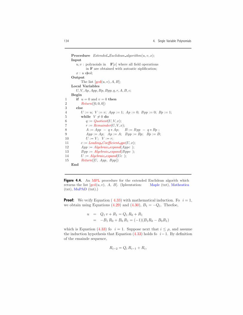
134 4. Single Variable Polynomials
Procedure Extended Euclidean algorithm(u, v, x);Input
u, v : polynomials in F[x] where all field operationsin F are obtained with automatic simplification;
x : a symbol;Output
The list [gcd(u, v), A,B];Local Variables
U, V,Ap,App,Bp,Bpp, q, r,A,B, c;Begin
1 if u = 0 and v = 0 then2 Return([0, 0, 0])3 else4 U := u; V := v; App := 1; Ap := 0; Bpp := 0; Bp := 1;5 while V �= 0 do6 q := Quotient(U, V, x);7 r := Remainder(U, V, x);8 A := App − q ∗ Ap; B := Bpp − q ∗ Bp ;9 App := Ap; Ap := A; Bpp := Bp; Bp := B;10 U := V ; V := r;11 c := Leading Coefficient gpe(U, x);12 App := Algebraic expand(App/c);13 Bpp := Algebraic expand(Bpp/c);14 U := Algebraic expand(U/c);15 Return([U, App, Bpp])
End
Figure 4.4. An MPL procedure for the extended Euclidean algorithm whichreturns the list [gcd(u, v), A, B]. (Implementation: Maple (txt), Mathematica(txt), MuPAD (txt).)
Proof: We verify Equation (4.33) with mathematical induction. For i = 1,we obtain using Equations (4.29) and (4.30), B1 = −Q1. Therefore,
u = Q1 v +R1 = Q1 R0 +R1
= −B1 R0 +B0 R1 = (−1)(B1R0 −B0R1)
which is Equation (4.33) for i = 1. Suppose next that i ≤ ρ, and assumethe induction hypothesis that Equation (4.33) holds for i−1. By definitionof the remainder sequence,
Ri−2 = QiRi−1 +Ri,
4.2. Greatest Common Divisors in F[x] 135
and from Equation (4.30)
Bi−2 = Bi +QiBi−1.
Using these relationships and the induction hypothesis, we have
u = (−1)i−1 (Bi−1 Ri−2 −Bi−2 Ri−1)= (−1)i−1 (Bi−1 (QiRi−1 +Ri)− (Bi +QiBi−1)Ri−1)= (−1)i (BiRi−1 −Bi−1 Ri)
which verifies the relationship for i. �
One way to find the cofactors cof(gcd(u, v), u) and cof(gcd(u, v), v) isto divide u and v by gcd(u, v). It is also possible to obtain them using therelationships in the next theorem.
Theorem 4.32. Let u and v be non-zero polynomials in F[x]. Then
cof(gcd(u, v), u) = (−1)ρBρ lc(Rρ−1),cof(gcd(u, v), v) = (−1)ρ−1Aρ lc(Rρ−1).
Proof: Since Rρ = 0 and gcd(u, v) = Rρ−1/lc(Rρ−1), these relationshipsfollow directly from Equations (4.33) and (4.34). �
Example 4.33. Let u = x7 − 4 x5 − x2 + 4 and v = x5 − 4 x3 − x2 + 4. Thegreatest common divisor of these polynomials is given in Example 4.24 asgcd(u, v) = R2 = x3 − x2 − 4 x + 4 with ρ = 3. The sequences Ai and Biare given in Example 4.28 where
A3 = x2 + x+ 1, B3 = −x4 − x3 − x2 − x− 1.
Therefore,
cof(gcd(u, v), u) = (−1)3B3 lc(R2) = x4 + x3 + x2 + x+ 1,cof(gcd(u, v), v) = (−1)2A3 lc(R2) = x2 + x+ 1. �
In Example 4.28, the degrees of the sequences Ai and Bi increase with i.In the next theorem we substantiate this observation.
Theorem 4.34. Let u and v be non-zero polynomials in F[x].
1. If ρ ≥ 2, then deg(A1) < deg(A2) < · · · < deg(Aρ).
136 4. Single Variable Polynomials
2. If ρ ≥ 2 and Q1 �= 0, then deg(B1) < deg(B2) < · · · < deg(Bρ).
3. If ρ ≥ 3 and Q1 = 0, then deg(B2) < deg(B3) < · · · < deg(Bρ).
Proof: We prove the theorem for the sequence Ai using mathematicalinduction. First, according to Exercise 3, deg(Qi) > 0 for i = 2, 3, . . . , ρ.Now, since A1 = 1 andA2 = −Q2, we have deg(A1) < deg(A2), and so thedegree relation holds for the base case i = 2. Let’s suppose that 3 ≤ i ≤ ρ,and assume the induction hypothesis that deg(Ai−2) < deg(Ai−1). Thisinequality together with Theorem 4.1(2) implies that
deg(Ai−2) < deg(Qi) + deg(Ai−1) = deg(QiAi−1),
which in turn implies that
deg(Ai−2−QiAi−1) = max({ deg(Ai−2), deg(QiAi−1)}) = deg(QiAi−1).
Finally, this relation together with the recurrence relation (4.30) gives
deg(Ai−1) < deg(Qi) + deg(Ai−1)= deg(QiAi−1)= deg(Ai−2 −QiAi−1)= deg(Ai)
which is the degree relation for i.The proof of the degree relationships for the sequence Bi is left to the
reader (Exercise 7). In this case the initial step for the induction dependson whether or not Q1 = 0. �
Using the previous theorem we have the following important result.
Theorem 4.35. Let u and v be polynomials in F[x] with positive degree.Then, deg(A) < deg(v) and deg(B) < deg(u).
Proof: First assume that ρ = 1. In this case v|u, and so gcd(u, v) =v/lc(v). Therefore, A = 0 and B = 1/lc(v) which implies that deg(A) <deg(v) and deg(B) < deg(u).Next suppose that ρ ≥ 2. Since A = Aρ−1/lc(Rρ−1), we have by Theo-
rem 4.32 and Theorem 4.34:
deg(A) = deg(Aρ−1)< deg(Aρ)≤ deg((−1)ρ−1Aρ lc(Rρ−1) gcd(u, v))= deg(v).

4.2. Greatest Common Divisors in F[x] 137
A similar argument shows that deg(B) < deg(v) when ρ ≥ 2, althoughthe case with ρ = 2 and Q1 = 0 is handled separately. �
Uniqueness of A and BThe polynomials A = Aρ−1/lc(Rρ−1) and B = Bρ−1/lc(Rρ−1) are not theonly ones that satisfy Equation (4.26). Indeed, if w is any polynomial,define
A′ = A+ w v, B′ = B − wu.
Then,
A′ u+B′ v = (A+ w v)u+ (B − wu) v = Au+B v = gcd(u, v).
However, when u and v are relatively prime, we have the following unique-ness result.
Theorem 4.36. Let u and v be polynomials in F[x] with positive degree, andsuppose that gcd(u, v) = 1. Then the polynomials A and B obtained withthe extended Euclidean algorithm are the only polynomials with deg(A) <deg(v) and deg(B) < deg(u) such that Au+B v = 1.
Proof: The existence of A and B is guaranteed by Theorem 4.35. To showthe uniqueness property, suppose that there are two pairs of polynomialsA, B and A′, B′ that satisfy the degree properties. Then, Au+B v = 1 =A′ u+B′ v, and
(A−A′)u = (B′ −B) v.
Since u divides the left side of this equation, it must also divide theright side. Therefore, since gcd(u, v) = 1, Theorem 4.29(1) implies thatu|B′ −B. However, since
deg(B′ −B) < deg(u),
we have B′ −B = 0. In a similar way A′ −A = 0. �
Example 4.37. The preceding theorem is not true when u and v have acommon factor with positive degree. For example, for u = x2 − 1 andv = x2 + 2 x+ 1, then
gcd(u, v) = R1/lc(R1) = x+ 1, A = −1/2, B = 1/2.
However, the polynomials A′ = x/2 and B′ = −x/2 + 1 also satisfy thedegree requirements, and A′ u + B′ v = x + 1. In fact, there are infinitely

138 4. Single Variable Polynomials
many pairs of polynomials A′ and B′ that satisfy these conditions (Exer-cise 13). This example is not just a rare occurrence but is indicative of theunderlying theory. We show in Chapter 7 that whenever u and v are notrelatively prime, this non-uniqueness property appears. �
Factorization of Polynomials
An important application of Theorem 4.27 is the following factorizationtheorem for polynomials.5
Theorem 4.38. Let u be a polynomial in F[x] with deg(u) > 0. Then, ucan be factored as
u = c p1 p2 · · · pr, (4.35)
where c is in F and each pi is a monic, irrreducible polynomial in F[x] withdeg(pi) > 0. The factorization is unique up to the order of the polynomi-als. The factorization (4.35) is called the irreducible factorization of uin F[x].
In other words, the uniqueness property states that two factorizationswith the factors pi listed in different orders are considered the same factor-ization.
Example 4.39. In Q[x] we have the unique factorization
2 x2 + 10 x+ 12 = 2 (x+ 2) (x+ 3).
An irreducible factorization depends on the field of coefficients. For exam-ple, u = x2 − 2 is irrreducible in Q[x] but can be factored as x2 − 2 =(x +
√2) (x − √2) in Q
(√2)[x]. Another example is x2 + 1 which is
irrreducible in Q[x] and Z3[x], but can be factored as
x2 + 1 = (x+ ı)(x− ı), in Q(ı)[x],x2 + 1 = (x+ 1)2, in Z2[x],x2 + 1 = (x+ 2)(x+ 3), in Z5[x]. �
Proof of Theorem 4.38: First, if u is irrreducible, then its irreduciblefactorization is given by
u = lc(u) p,
where p is the monic polynomial with coefficients obtained from the coef-ficients of u divided by lc(u).
5Theorem 4.27 is applied through Theorem 4.29(2) which follows from Theorem 4.27.

4.2. Greatest Common Divisors in F[x] 139
Next, if u is reducible, it can be factored u = v w where 0 < deg(v) <deg(u) and 0 < deg(w) < deg(u). If v and w are irrreducible, the processterminates. If not, the process continues by factoring v and w. Theorem4.1(2) implies that the process eventually terminates with the factorization
u = q1 q2 · · · qr, (4.36)
where each qi is irrreducible and 0 < deg(qi) < deg(u). In addition,
u = q1 q2 · · · qr = c p1 p2 · · · prwhere
c = lc(q1) lc(q2) · · · lc(qr),and pi is an irrreducible monic polynomial with coefficients obtained fromthe coefficients of qi divided by lc(qi).
To show the uniqueness of the factorization, suppose that u has twoirreducible factorizations
u = c p1 p2 · · · pr = c′ p′1 p′2 · · · p′s. (4.37)
Since c = lc(u) = c′, we divide both factorizations by the leading coefficientto obtain
p1 p2 · · · pr = p′1 p′2 · · · p′r′ . (4.38)
Now, since the irrreducible polynomial p1 divides the both sides of Equation(4.38), it divides some factor p′j on the right (Theorem 4.29(2)). In fact,since both polynomials are monic and irrreducible, pi = p′j . Dividing bothsides of Equation (4.38) by this polynomial, we obtain
p2 p3 · · · pr = p′1 p′2 · · · p′j−1 p
′j+1 · · · p′r′ .
Repeating this argument for each successive polynomial pi, i = 2, . . . , r, itfollows that r = r′ and each polynomial pi corresponds to a unique polyno-mial on the right side of Equation (4.37). Therefore, the two factorizationsare the same except for a possible rearrangement of the factors. �
By combining like factors in the previous theorem we obtain the follow-ing theorem.
Theorem 4.40. Let u be a polynomial in F[x] with deg(u) > 0. Then, ucan be factored uniquely as
u = c pn11 pn2
2 · · · pnss ,
where the polynomials pi are monic, irrreducible, and relatively prime.

140 4. Single Variable Polynomials
Theorems 4.38 and 4.40 are “non-constructive” mathematical state-ments because they assert the existence of a unique factorization but donot give an algorithm to compute it. In Chapter 9 we describe algorithmsthat obtain the irreducible factorization of polynomials in Q[x].
Chinese Remainder Problem in F[x]
The next theorem, which is also based on the extended Euclidean algo-rithm, is the polynomial version of the Chinese Remainder Theorem.
Theorem 4.41. Let u1, u2, . . . , ur be polynomials in F[x] with positive de-gree that are pairwise relatively prime, and let a1, a2, . . . , ar be polynomialsin F[x] with deg(ai) < deg(ui). Then, there is exactly one h in F[x] with
deg(h) < deg(u1) + · · ·+ deg(ur) (4.39)
that satisfies the remainder equations
rem(h, ui) = ai, i = 1, 2, . . . , r. (4.40)
Proof: We prove the theorem with mathematical induction. First, for thebase case r = 1, the division property for polynomials implies that h = a1.Let’s assume now that there is a polynomial z that satisfies the remainderequations
rem(z, ui) = ai, i = 1, . . . , r − 1, (4.41)
with deg(z) < deg(u1)+· · ·+deg(ur−1) and show how to extend the processone step further to find a polynomial h that satisfies the conditions in thetheorem. Observe that the condition (4.41) implies that
z = qi ui + ai, i = 1, . . . , r − 1, (4.42)
where qi = quot(z, ui). In addition, for v = u1 · · ·ur−1, the pairwise rela-tively prime hypothesis in the theorem implies that gcd(v, ur) = 1. Now,using the extended Euclidean algorithm, we obtain polynomials A and Bsuch that
Av +B ur = 1. (4.43)
Let
g = Av ar +B ur z, (4.44)u = v ur = u1 · · ·ur.
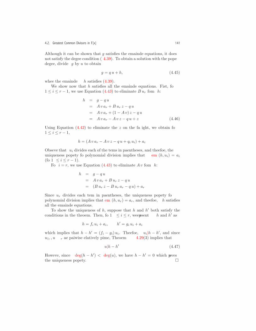
4.2. Greatest Common Divisors in F[x] 141
Although it can be shown that g satisfies the remainder equations, it doesnot satisfy the degree condition (4.39). To obtain a solution with the properdegree, divide g by u to obtain
g = q u+ h, (4.45)
where the remainder h satisfies (4.39).We show now that h satisfies all the remainder equations. First, for
1 ≤ i ≤ r − 1, we use Equation (4.43) to eliminate B ur from h:
h = g − q u
= Av ar +B ur z − q u
= Av ar + (1 −Av) z − q u
= Av ar −Av z − q u+ z. (4.46)
Using Equation (4.42) to eliminate the z on the far right, we obtain for1 ≤ i ≤ r − 1,
h = (Av ar −Av z − q u+ qi ui) + ai.
Observe that ui divides each of the terms in parentheses, and therefore, theuniqueness property for polynomial division implies that rem(h, ui) = ai(for 1 ≤ i ≤ r − 1).
For i = r, we use Equation (4.43) to eliminate Av from h:
h = g − q u
= Av ar +B ur z − q u
= (B ur z −B ur ar − q u) + ar.
Since ur divides each term in parentheses, the uniqueness property forpolynomial division implies that rem(h, ur) = ar, and therefore, h satisfiesall the remainder equations.
To show the uniqueness of h, suppose that h and h′ both satisfy theconditions in the theorem. Then, for 1 ≤ i ≤ r, we represent h and h′ as
h = fi ui + ai, h′ = gi ui + ai
which implies that h − h′ = (fi − gi)ui. Therefore, ui|h − h′, and sinceu1, . . . , ur are pairwise relatively prime, Theorem 4.29(3) implies that
u|h− h′. (4.47)
However, since deg(h − h′) < deg(u), we have h − h′ = 0 which provesthe uniqueness property. �
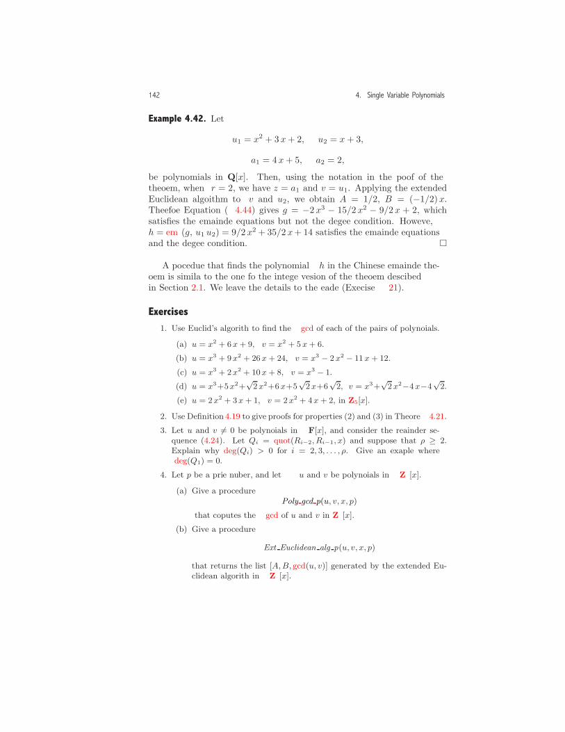
142 4. Single Variable Polynomials
Example 4.42. Let
u1 = x2 + 3 x+ 2, u2 = x+ 3,
a1 = 4 x+ 5, a2 = 2,
be polynomials in Q[x]. Then, using the notation in the proof of thetheorem, when r = 2, we have z = a1 and v = u1. Applying the extendedEuclidean algorithm to v and u2, we obtain A = 1/2, B = (−1/2)x.Therefore Equation (4.44) gives g = −2 x3 − 15/2 x2 − 9/2 x + 2, whichsatisfies the remainder equations but not the degree condition. However,h = rem(g, u1 u2) = 9/2 x2 + 35/2 x+ 14 satisfies the remainder equationsand the degree condition. �
A procedure that finds the polynomial h in the Chinese remainder the-orem is similar to the one for the integer version of the theorem describedin Section 2.1. We leave the details to the reader (Exercise 21).
Exercises1. Use Euclid’s algorithm to find the gcd of each of the pairs of polynomials.
(a) u = x2 + 6x + 9, v = x2 + 5 x + 6.
(b) u = x3 + 9x2 + 26x + 24, v = x3 − 2 x2 − 11 x + 12.
(c) u = x3 + 2x2 + 10x + 8, v = x3 − 1.
(d) u = x3+5x2+√
2x2+6x+5√
2x+6√
2, v = x3+√
2x2−4x−4√
2.
(e) u = 2x2 + 3x + 1, v = 2x2 + 4x + 2, in Z5[x].
2. Use Definition 4.19 to give proofs for properties (2) and (3) in Theorem 4.21.
3. Let u and v �= 0 be polynomials in F[x], and consider the remainder se-quence (4.24). Let Qi = quot(Ri−2, Ri−1, x) and suppose that ρ ≥ 2.Explain why deg(Qi) > 0 for i = 2, 3, . . . , ρ. Give an example wheredeg(Q1) = 0.
4. Let p be a prime number, and let u and v be polynomials in Zp[x].
(a) Give a procedurePoly gcd p(u, v, x, p)
that computes the gcd of u and v in Zp[x].
(b) Give a procedure
Ext Euclidean alg p(u, v, x, p)
that returns the list [A,B, gcd(u, v)] generated by the extended Eu-clidean algorithm in Zp[x].
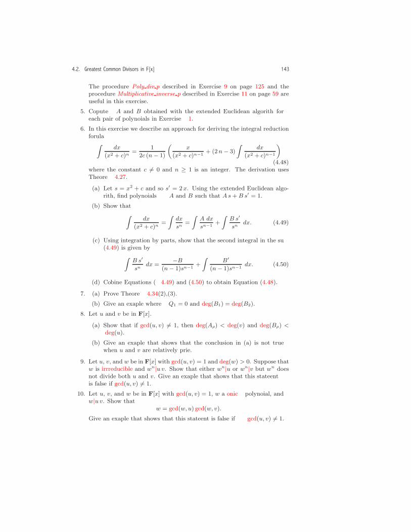
4.2. Greatest Common Divisors in F[x] 143
The procedure Poly div p described in Exercise 9 on page 125 and theprocedure Multiplicative inverse p described in Exercise 11 on page 59 areuseful in this exercise.
5. Compute A and B obtained with the extended Euclidean algorithm foreach pair of polynomials in Exercise 1.
6. In this exercise we describe an approach for deriving the integral reductionformula
dx
(x2 + c)n=
1
2c (n− 1)
x
(x2 + c)n−1+ (2n− 3)
dx
(x2 + c)n−1
(4.48)where the constant c �= 0 and n ≥ 1 is an integer. The derivation usesTheorem 4.27.
(a) Let s = x2 + c and so s′ = 2x. Using the extended Euclidean algo-rithm, find polynomials A and B such that As + B s′ = 1.
(b) Show that
dx
(x2 + c)n=
dx
sn=
A dx
sn−1+
B s′
sndx. (4.49)
(c) Using integration by parts, show that the second integral in the sum(4.49) is given by
B s′
sndx =
−B
(n− 1)sn−1+
B′
(n− 1)sn−1dx. (4.50)
(d) Combine Equations (4.49) and (4.50) to obtain Equation (4.48).
7. (a) Prove Theorem 4.34(2),(3).
(b) Give an example where Q1 = 0 and deg(B1) = deg(B2).
8. Let u and v be in F[x].
(a) Show that if gcd(u, v) �= 1, then deg(Aρ) < deg(v) and deg(Bρ) <deg(u).
(b) Give an example that shows that the conclusion in (a) is not truewhen u and v are relatively prime.
9. Let u, v, and w be in F[x] with gcd(u, v) = 1 and deg(w) > 0. Suppose thatw is irrreducible and wn|u v. Show that either wn|u or wn|v but wn doesnot divide both u and v. Give an example that shows that this statementis false if gcd(u, v) �= 1.
10. Let u, v, and w be in F[x] with gcd(u, v) = 1, w a monic polynomial, andw|u v. Show that
w = gcd(w, u) gcd(w, v).
Give an example that shows that this statement is false if gcd(u, v) �= 1.

144 4. Single Variable Polynomials
11. Let u, v, and w �= 0 be in F[x]. Show that
gcd(wu, w v) = w/lc(w) gcd(u, v).
12. Let u v, and w be in F[x] with gcd(u, v) = 1. Show that
gcd(w, u v) = gcd(w, u) gcd(w, v).
Give an example that shows that this statement is false if gcd(u, v) �= 1.
13. Suppose that u = x2 − 1 and v = x2 + 2 x + 1 where gcd(u, v) = x + 1.Show that there are infinitely many pairs of polynomials A and B whereAu + B v = x + 1 and deg(A) < deg(v), deg(B) < deg(u).
14. Let u and v be relatively prime and have positive degree, and suppose thatS and T are two polynomials such that S u + T v = 1. (S and T are notnecessarily the ones generated by the extended Euclidean algorithm.) LetA = rem(S, v) and B = rem(T, u). Show that A and B are the polynomialsobtained with the extended Euclidean algorithm.
15. Let u and v be polynomials in F[x] with positive degree. Show thatgcd(u, v) �= 1 if and only if there are polynomials C and D with deg(C) <deg(v) and deg(D) < deg(u) such that C u = D v.
16. In this problem, p and u are polynomials in Q[x] where p is irrreducibleand u′ is the derivative of u.
(a) Suppose that u = pn w. Show that pn−1|gcd(u, u′).
(b) Now show the converse of Part (a). Suppose that pn−1|gcd(u, u′).Show that pn|u.
17. Let u, v and w be in F[x] where u and v have positive degree, gcd(u, v) = 1,and deg(w) < deg(u)+deg(v). Show there are unique polynomials C and Din F[x] with deg(C) < deg(v) and deg(D) < deg(u) such that C u+ Dv =w.
18. In this exercise we describe a simple version of a rational simplificationoperator. The operator is applied to expressions in the class RS-IN (whereIN refers to “input”) that satisfy one of the following rules.
RS-IN-1. u is an integer.
RS-IN-2. u is a fraction.
RS-IN-3. u is the symbol x.
RS-IN-4. u is a sum with operands that are in RS-IN.
RS-IN-5. u is a product with operands that are in RS-IN.
RS-IN-6. u = vn, where v is in RS-IN, and n is an integer.
The goal is to transform u to a rational expression v in Q(x) in a standardform that satisfies one of the following rules.

4.2. Greatest Common Divisors in F[x] 145
RS-1. v is a polynomial in Q[x].
RS-2. For n = Numerator(v) and d = Denominator(v), n and d are monicpolynomials in Q[x] which satisfy the following conditions.
(a) d has positive degree.
(b) n and d are relatively prime as polynomials in Q[x].
RS-3. v = cw where c is a rational number and w satisfies RS-2.
(a) Give a procedure for Rational simplify sv(u, x) (where the suffix “sv”stands for “single variable”) that either returns the standard form of uor the global symbol Undefined if a division by zero is encountered.For example,
Rational simplify svx2 − 1
x + 1, x → x− 1,
Rational simplify svx + 1
x2 − 1 − (x + 1) ∗ (x− 1), x →Undefined,
Rational simplify sv1
1 + 1x+1
+2
x + 2, x → x + 3
x + 2,
Rational simplify sv2x + 4
3x + 9, x → (2/3)
x + 2
x + 3.
(b) For a CAS, the standard form for a rational expression may be differ-ent from the one given above. Experiment with a CAS to determinethe standard form for rationally simplified expressions in Q(x). (Usenormal in Maple and MuPAD and Together in Mathematica.) Onpage 257 we describe another standard form for rational expressions.
19. Find the irreducible factorization of each of the following polynomials inZ5[x].
(a) x2 + 2x + 2.
(b) x3 + 1.
20. Consider the polynomial (−1 + 5 ı)x2 + (9 + 8 ı)x + (3 − 6 ı) in (Q(ı))[x].Factor the polynomial in the form (4.35).
21. Let A = [a1, . . . , ar] and U = [u1, . . . , ur] be lists of polynomials in Q[x]that satisfy the conditions in the Chinese Remainder Theorem (Theorem4.41). Give a procedure Poly Chinese rem(A,U, x) that obtains the poly-nomial h described in the theorem.
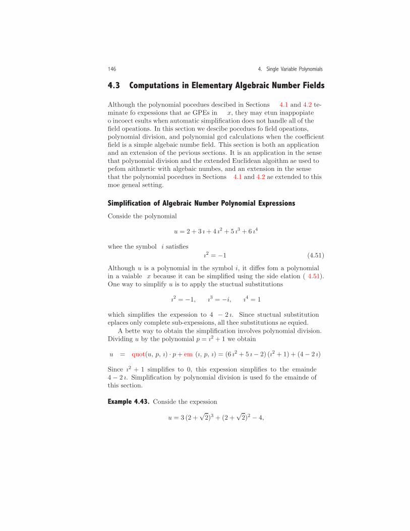
146 4. Single Variable Polynomials
4.3 Computations in Elementary Algebraic Number Fields
Although the polynomial procedures described in Sections 4.1 and 4.2 ter-minate for expressions that are GPEs in x, they may return inappropriateor incorrect results when automatic simplification does not handle all of thefield operations. In this section we describe procedures for field operations,polynomial division, and polynomial gcd calculations when the coefficientfield is a simple algebraic number field. This section is both an applicationand an extension of the previous sections. It is an application in the sensethat polynomial division and the extended Euclidean algorithm are used toperform arithmetic with algebraic numbers, and an extension in the sensethat the polynomial procedures in Sections 4.1 and 4.2 are extended to thismore general setting.
Simplification of Algebraic Number Polynomial Expressions
Consider the polynomial
u = 2 + 3 ı+ 4 ı2 + 5 ı3 + 6 ı4
where the symbol i satisfiesı2 = −1. (4.51)
Although u is a polynomial in the symbol i, it differs from a polynomialin a variable x because it can be simplified using the side relation (4.51).One way to simplify u is to apply the structural substitutions
ı2 = −1, ı3 = −i, ı4 = 1
which simplifies the expression to 4 − 2 ı. Since structural substitutionreplaces only complete sub-expressions, all three substitutions are required.
A better way to obtain the simplification involves polynomial division.Dividing u by the polynomial p = ı2 + 1 we obtain
u = quot(u, p, ı) · p+ rem(ı, p, ı) = (6 ı2 + 5 ı− 2) (ı2 + 1) + (4− 2 ı).
Since ı2 + 1 simplifies to 0, this expression simplifies to the remainder4 − 2 ı. Simplification by polynomial division is used for the remainder ofthis section.
Example 4.43. Consider the expression
u = 3 (2 +√2)3 + (2 +
√2)2 − 4,
4.3. Computations in Elementary Algebraic Number Fields 147
and let’s view u as a polynomial in the algebraic number x = 2+√2, which
satisfies the side relation f(x) = x2 − 4 x+ 2 = 0. The simplified form of uis given by
u = rem(u(α), f(α), α) = −30 + 46α (4.52)
= −30 + 46 (2 +√2). (4.53)
In fact, the general relation in Equation (4.52) holds for any root of f(x) =0. For example, for the root α = 2−√2, we also have the simplification
3 (2−√2)3 + (2 −√2)2 − 4 = −30 + 46 (2−√2). �
The Minimal Polynomial of an Algebraic Number
Let α be an algebraic number that is a root of the polynomial equationf(x) = 0, where f is in Q[x] and deg(f) ≥ 2. In order to simplify apolynomial u(α), we must divide u by the simplest polynomial that has αas a root. This polynomial is described in the following theorem.
Theorem 4.44. Let α be an algebraic number. Then, there is a unique,monic, irrreducible polynomial p(x) �= 0 in Q[x] such that p(α) = 0. Thepolynomial p is called the minimal polynomial of α.
Proof: Suppose that α is a root of the polynomial equation f(x) = 0.Then f can be factored as f(x) = c · p1(x) · p2(x) · · · pn(x), where each piis a monic and irrreducible polynomial in Q[x]. Since f(α) = 0, α is theroot of one of these polynomials, say pi′ . Let p = pi′ .
To show that p is the only polynomial with these properties, we firstshow that p is a divisor of any (non-zero) polynomial g(x) in Q[x] thathas α as a root. Since p is irrreducible, the two polynomials p and g areeither relatively prime or p|g. We show that the first of these two optionsis impossible.
If p and g were relatively prime, then, by the extended Euclidean algo-rithm, there are polynomials A(x) and B(x) in Q[x] such that
A(x) p(x) +B(x) g(x) = gcd(g, p) = 1. (4.54)
Substituting x = α into this expression, we obtain
A(α) p(α) +B(α) g(α) = A(α) · 0 +B(α) · 0 = 0. (4.55)
Since Equations (4.54) and (4.55) cannot both be true (0 �= 1), p and gcannot be relatively prime, and so p|g. Therefore, if g is a polynomial

148 4. Single Variable Polynomials
which satisfies the three properties in the theorem ( monic, irrreducible,g(α) = 0), we must have p = g. �
Example 4.45. In order to find the simplest form of u(α) using polyno-mial division, the side relation associated with α must be the minimalpolynomial. For example, let α = ı and
u = 2 + 3 ı+ 4 ı2 + 5 ı3 + 6 ı4.
The minimal polynomial of ı is p(x) = x2 + 1. Of course ı is also a root ofany multiple of p(x) such as
f(x) = (x2 + 1) (x− 1) = x3 − x2 + x− 1.
However,rem(u, f(ı), ı)→ 9 ı2 − 2 ı+ 13,
rather than the simplified form
rem(u, ı2 + 1, ı) = 4− 2 ı. �
Arithmetic in Algebraic Number Fields
In Section 2.3 we described a number of fields that are constructed byadjoining an algebraic number to the rational numbers Q (e.g., Q(ı)). Inthe next definition and theorem we describe a systematic approach forarithmetic in this setting.
Definition 4.46. Let α be an algebraic number with minimal polynomial psuch that deg(p, x) = n ≥ 2, and let Q(α) be the set of polynomials u inQ[α] such that deg(u, α) < n. For polynomials u(α) and v(α) in Q(α),define an addition operation as ordinary polynomial addition
u+ v,
and a multiplication operation as
rem(u · v, p(α), α).
Notice that with these operations both the sum and product of poly-nomials in Q(α) are in simplified form with respect to the side relationp(α) = 0.

4.3. Computations in Elementary Algebraic Number Fields 149
Example 4.47. Let α = 21/3. Since the minimal polynomial of α is p(x) =x3 − 2, the set Q(α) consists of polynomials of the form a + b α + c α2,where a, b, and c are rational numbers. Let
u = 1 + α+ 2α2, v = 2− α+ 3α2.
Using the operations described in Definition 4.46, the sum of u and v is
u+ v = 3 + 5α2,
and the product is
rem(u · v, p(α), α) = rem(2 + α+ 6α2 + α3 + 6α4, α3 − 2, α)= 4 + 13α+ 6α2. �
Theorem 4.48. The set Q(α) with the addition and multiplication opera-tions described in Definition 4.46 is a field.
Proof: The addition and multiplication operations are defined so thatthe closure axioms (F-1 and F-2) are automatically satisfied, and using theproperties of polynomials, the field axioms F-3 through F-11 are also easyto verify.
To show that Q(α) is a field, we need only show that each field elementu(α) �= 0 has a multiplicative inverse (Axiom F-12). Since the minimalpolynomial p is irrreducible with deg(u) < deg(p), and since u(α) �= 0, wehave gcd(u(α), p(α)) = 1. By the extended Euclidean algorithm, there arepolynomials A(α) and B(α) such that
A(α)u(α) +B(α) p(α) = 1 (4.56)
where, by Theorem 4.36, deg(A) < deg(p). To show that A(α) is themultiplicative inverse of u(α), we compute the product of A(α) and u(α)in Q(α). Using Equation (4.56), we have
rem(A(α)u(α), p(α), α) = rem(1−B(α) p(α), p(α), α) = 1.
Therefore, A is the multiplicative inverse of u, and Q(α) is a field. �
Example 4.49. Consider the field Q(21/3), where the minimal polynomialof α = 21/3 is p(x) = x3 − 2. Let u = 2 + 3 · 21/3. Applying the extendedEuclidean algorithm we obtain

150 4. Single Variable Polynomials
u−1 = A = 9/62α2 − 3/31α+ 2/31,
and therefore,(2 + 3 · 21/3
)−1
= 9/62 · 22/3 − 3/31 · 21/3 + 2/31.
In fact, A is the inverse for all solutions α of x3 − 2 = 0. For example,another solution is
α = 21/3
(−12+
31/2 ı
2
),
and so(21/3
(−12+
31/2 ı
2
))−1
= 9/62 ·(21/3
(−12+
31/2 ı
2
))2
− 3/31 ·(21/3
(−12+
31/2 ı
2
))+2/31. �
Procedures for the Field Operations in Q(α). Addition of u and v in Q(α)is obtained with automatic simplification, and the additive inverse of u isobtained with6
Algebraic expand(−1 · u).Multiplication in Q(α) is given by
Remainder(Algebraic expand(u · v), p, α),
where the minimal polynomial is expressed in terms of the symbol α insteadof the symbol x.
Procedures for the multiplicative inverse and division operations aregiven in Figure 4.5. The multiplicative inverse is obtained in the procedureAlg mult inverse with the extended Euclidean algorithm (line 1).
A general simplifier for expressions constructed from integers, fractions,the algebraic number α, sums, products, and powers with integer exponentsis described in Exercise 4.
Procedures for Polynomial Operations in Q(α)[x]. Let’s consider now the ex-tension of the polynomial operations described in Sections 4.1 and 4.2 forpolynomials in Q(α)[x].
6In a computer algebra system where −1 is distributed over a sum by automaticsimplification, the Algebraic expand operator can be omitted.

4.3. Computations in Elementary Algebraic Number Fields 151
Procedure Alg mult inverse(v, p, α);Input
α : a symbol that represents an algebraic number;p : a monic, irrreducible polynomial in Q[α] with deg(p, α) ≥ 2;v : a non-zero polynomial in Q(α) with deg(v) < deg(p);
OutputThe multiplicative inverse of v in Q(α);
Local Variablesw;
Begin1 w := Extended Euclidean algorithm(v, p, α);2 Return(Operand(w, 2))
End
Procedure Alg divide(u, v, p, α);Input
α : a symbol that represents an algebraic number;p : a monic, irrreducible polynomial in Q[α] with deg(p, α) ≥ 2;u, v : polynomials in Q(α) with degree < deg(p) and v �= 0;
OutputThe quotient of u divided by v in Q(α);
Local Variablesw;
Begin1 w := Alg mult inverse(v, p, α);2 Return(Remainder(Algebraic expand(u ∗ w), p, α))
End
Figure 4.5. MPL procedures for the division and multiplicative inverse operationsin Q(α). In both procedures, the minimal polynomial is expressed in terms of thesymbol α rather than the symbol x. (Implementation: Maple (txt), Mathematica(txt), MuPAD (txt).)
The polynomial division procedure7 shown in Figure 4.6 is a modifica-tion of the one given in Figure 4.1 on page 116.
Observe that at line 8, we obtain the quotient lcr/lcv with the Alg divideoperator. At line 10, the product of the algebraic number s with thecoefficients of v may give coefficients that are unsimplified with respect top(α) = 0 (see Example 4.50). For this reason, the operator Alg coeff simpis included at line 11 to simplify each of the (algebraic number) coefficientsof the polynomial (Exercise 2).
7See the comment concerning the MuPAD implementation in footnote 2 on page 115.

152 4. Single Variable Polynomials
Procedure Alg polynomial division(u, v, x, p, α);Input
u, v : polynomials in Q(α)[x] with v �= 0;x : a symbol;α : a symbol that represents an algebraic number;p : a monic, irrreducible polynomial in Q[α] with degree ≥ 2;
OutputA list [q, r] with the quotient and remainder;
Local Variablesq, r,m,n, lcv, lcr, s;
Begin1 q := 0;2 r := u;3 m := Degree gpe(r, x);4 n := Degree gpe(v, x).5 lcv := Leading Coefficient gpe(v, x);6 while m ≥ n do7 lcr := Leading Coefficient gpe(r, x);8 s := Alg divide(lcr, lcv, p, α);9 q := q + s ∗ xm−n;10 r := Algebraic expand (r − lcr ∗ xm) − (v − lcv xn) ∗ s ∗ xm−n ;11 r := Alg coeff simp(r, x, p, a);12 m := Degree gpe(r, x);13 Return([q, r])
End
Alg quotient(u, v, x, p, α)function
:=
Operand(Alg polynomial division(u, v, x, p, α), 1);
Alg remainder(u, v, x, p, α)function
:=
Operand(Alg polynomial division(u, v, x, p, α), 2);
Figure 4.6. An MPL procedure for polynomial division in Q(α)[x] and func-tions that extract the quotient and remainder. (Implementation: Maple (txt),Mathematica (txt), MuPAD (txt).)

4.3. Computations in Elementary Algebraic Number Fields 153
Example 4.50. Let α be a root of p(x) = x2 − 2 = 0, and consider thepolynomials in Q(α)[x]:
u = 2 x2 + αx, v = αx+ α.
Let’s consider the division of u by v using the Alg polynomial division pro-cedure. The quotient and remainder are initialized at lines 1–2 with
q = 0, r = 2 x2 + αx.
On the first pass through the loop, we have
s =2α= α, q = αx,
andr = xα− α2 x = (α− 2)x,
where the middle expression is the unsimplified form from line 10 and theexpression on the right is the simplified form from line 11. On the secondpass, we have
s =α− 2α
= 1− α, q = αx+ 1− α,
andr = −α+ α2 = −α+ 2,
where again the middle expression is the unsimplified form and the ex-pression on the right is the simplified form. At this point, the processterminates with quotient q = αx+ 1− α and remainder −α+ 2. �
A procedure that obtains the greatest common divisor8 inQ(α)[x] basedon Euclid’s algorithm is given in Figure 4.7. The operator Alg monic inline 6 assures that the gcd is a monic polynomial (Exercise 3).
Example 4.51. Let α be a root of p(x) = x2 − 2 = 0 and consider thepolynomials in Q(α)[x]:
u = x2 + (−1− α)x, v = x2 + (−2− 2α)x+ 3 + 2α.
The remainder sequence produced by Alg polynomial gcd at line 3 is
R = x+ αx− 3− 2α, (4.57)R = 0.
8Another approach is suggested in Exercise 10, page 347.

154 4. Single Variable Polynomials
Procedure Alg polynomial gcd(u, v, x, p, α);Input
u, v : polynomials in Q(α)[x];x : a symbol;α : a symbol that represents an algebraic number;p : a monic, irrreducible polynomial in Q[α] with degree ≥ 2;
Outputgcd(u, v);
Local VariablesU,V, R;
Begin1 U := u; V := v;2 while V �= 0 do3 R := Alg remainder(U, V, x, p, α);4 U := V ;5 V := R;6 Return(Alg monic(U,x, p, α))
End
Figure 4.7. An MPL procedure for the Euclidean algorithm that computesgcd(u, v) in Q(α)[x]. (Implementation: Maple (txt), Mathematica (txt), MuPAD(txt).)
Therefore, using the remainder (4.57), at line 6 we obtain
gcd(u, v) = R/lc(R) = x− 1− α. �
In a similar way, we can modify the procedures for polynomial expansionand the extended Euclidean algorithm to handle polynomials in Q(α)[x](Exercises 5 and 6).
Multiple Algebraic Extensions
We consider now the arithmetic and polynomial operations when a finiteset {α1, α2, . . . , αs} of algebraic numbers is adjoined to Q. We begin withsome examples.
Example 4.52. Consider the simplification problem for a polynomial ex-pression in the two positive algebraic numbers α1 =
√2 and α2 =
√3,
which satisfy the two side relations
p1(x1) = x21 − 2 = 0, p2(x2) = x2
2 − 3 = 0.

4.3. Computations in Elementary Algebraic Number Fields 155
To simplify
u = 2 + 3α1 + 4α21 + α2 − α1 α2 + α2
1 α2 + 3α22 − α1 α
22 − 2α2
1 α22,
we view u as a polynomial in Q(α1)[α2]:
u = (2 + 3α1 + 4α21) + (1 − α1 + α2
1)α2 + (3− α1 − 2α21)α
22.
Simplifying the coefficients in parentheses by replacing each of them withthe remainder of division by p1(α1), we obtain
u = (10 + 3α1) + (3− α1)α2 + (−1− α1)α22.
The final simplification is the remainder obtained by dividing this polyno-mial (considered in Q(α1)[α2]) by p2(α2):
u = rem(u, p2(α2), α2) → 7 + (3− α1)α2
= 7 +(3−√2
) √3. �
Example 4.53. Consider the simplification problem for a polynomial ex-pression in the two positive algebraic numbers α1 =
√2 and α2 =
√8,
which satisfy the two side relations
p1(x1) = x21 − 2 = 0, p2(x2) = x2
2 − 8 = 0.
Letu = α1 α2 − 4,
and consider the problem of simplifying u. If we proceed as in the lastexample by dividing u by p2(α2), we obtain the remainder u = α1 α2 − 4rather than the simplified form u =
√2√8 − 4 = 0. The difficulty arises
because there is a dependence relation between√2 and
√8:
2α1 − α2 = 2√2−√8 = 0. �
The last example shows that when there is an algebraic relationshipbetween algebraic numbers, simplification with polynomial division by theminimal polynomials may not determine that an expression simplifies tozero. In the next definition we describe the form of these dependencerelations.
Definition 4.54. Let S = {α1, α2, . . . , αs} be algebraic numbers, and letpi(xi) be the minimal polynomial of αi. The set S is algebraically depen-dent if there exists a non-zero polynomial h(x1, x2, . . . , xs) with rationalnumber coefficients such that
deg(h, xi) < deg(pi, xi), for i = 1, 2, . . . , s (4.58)

156 4. Single Variable Polynomials
andh(α1, α2, . . . , αs) = 0. (4.59)
If the set S is not dependent, it is called algebraically independent.
In other words, a set S of algebraic numbers is algebraically dependent ifthere is a polynomial relation between the numbers. The degree condition(4.58) is essential because without it the definition is meaningless. Indeed,
h(x1, . . . , xs) = p1(x1) · · · p(xs)
satisfies Equation (4.59) but not the inequality (4.58).
Example 4.55. Consider the positive algebraic numbers α1 =√2 and
α2 =√8 with minimal polynomials p1(x1) = x2
1 − 2 and p2(x2) = x22 − 8.
These numbers are algebraically dependent with
h(x1, x2) = 2 x1 − x2.
Notice that the dependence relation depends on which roots of the minimalpolynomials are considered. For example, for α1 = −
√2 and α2 =
√8, the
dependence relation is
h(x1, x2) = 2 x1 + x2.
The positive algebraic numbers α1 =√2, α2 =
√3, and α3 =
√6 are
algebraically dependent with
h(x1, x2, x3) = x1 x2 − x3.
The positive algebraic numbers
α1 =√2, α2 =
√3, α3 =
√30 + 12
√6
are algebraically dependent with
h(x1, x2, x3) = 3 x1 + 2 x2 − x3.
The dependence relationship h(α1, α2, α3) = 0 can be verified by squaringboth sides of the equation
3√2 + 2
√3 =
√30 + 12
√6. �

4.3. Computations in Elementary Algebraic Number Fields 157
Example 4.56. The positive algebraic numbers α1 =√2 and α2 =
√3 are
algebraically independent. To show this we must show that it is impossibleto find a non-zero polynomial
h(x1, x2) = a+ b x1 + c x2 + d x1 x2, (4.60)
with a, b, c, and d rational numbers such that
h(α1, α2) = a+ b√2 + c
√3 + d
√2√3 = 0. (4.61)
First, if such a polynomial did exist, then both c and d cannot be zerobecause, if this were so, Equation (4.61) becomes
a+ b√2 = 0. (4.62)
In this expression, b �= 0 because, if this were not so, then a = 0 as well,and h(x1, x2) is the zero polynomial. On the other hand, if b �= 0, Equation(4.62) implies that
√2 is a rational number which, of course, is not true.
Therefore, we assume that either c or d is not zero which implies, usingthe above reasoning, that c + d
√2 �= 0. When this is so, Equation (4.61)
implies√3 =−a− b
√2
c+ d√2
,
and by rationalizing the denominator, we obtain√3 = e+ f
√2,
where e and f are rational numbers. Squaring both sides of this expression,we obtain
3 = e2 + 2 e f√2 + 2 f2. (4.63)
If both e �= 0 and f �= 0, then again we would conclude that√2 is a rational
number, and so either e or f is zero.Suppose that e = 0 and f = f1/f2 where f1 and f2 are integers with
no common factor. Then from Equation (4.63), we have
3 f22 = 2 f2
1 . (4.64)
Since 3 divides the left side of the equality, Theorem 2.16(2) implies that3|f2
1 , and then Theorem 2.16(1) implies that 3|f1. Therefore, 32|f21 , and by
Equation (4.64), 3|f22 . Again, Theorem 2.16(1) implies that 3|f2, and so we
conclude that f1 and f2 have a common factor, which is a contradiction.Therefore, e �= 0. In a similar way we can conclude that f �= 0.
Finally, since both e and f cannot be non-zero, the polynomial (4.60)does not exist, and so
√2 and
√3 are independent algebraic numbers. �

158 4. Single Variable Polynomials
The last example is a special case of the next theorem which gives alarge set of independent algebraic numbers.9
Theorem 4.57. Let n1, n2, . . . , ns be distinct prime numbers, and let m1,m2,. . . ,ms be integers that are ≥ 2. Then {n1/m1
1 , n1/m22 , . . . , n
1/mss } is an
set of independent algebraic numbers.
Arithmetic with Two Independent Algebraic Numbers
Definition 4.58. Let α1 and α2 be independent algebraic numbers withminimal polynomials p1(x1) and p2(x2) with rational number coefficientsand degree ≥ 2. Let
Q(α1, α2)
be the set of polynomials u in Q(α1)[α2] with deg(u, α2) < deg(p2(x2), x2).For u and v in Q(α1, α2), the addition operation is defined as ordinarypolynomial addition, and the multiplication operation is
rem(u · v, p2(α2), α2
),
where the remainder operation is performed in Q(α1)[α2].
For u �= 0, the multiplicative inverse is obtained with the extendedEuclidean algorithm in Q(α1)[x2] using an approach similar to what wasdone in the proof of Theorem 4.48. (See Example 4.60 and Exercise 6.)This approach requires that the minimal polynomial p2(x2) be irrreduciblein Q(α1)[x2]. Although p2(x2) is irrreducible as a polynomial in Q[x2],it is only irrreducible in the larger setting Q(α1)[x2] when α1 and α2 areindependent algebraic numbers. This is the content of the next theorem.
Theorem 4.59. Let α1 and α2 be algebraic numbers with minimal polynomialsp1(x1) and p2(x2). The polynomial p2(x2) is irrreducible in Q(α1)[x2] ifand only if α1 and α2 are algebraically independent.
Proof: First assume that α1 and α2 are algebraically independent. Let’ssuppose that p2 were reducible as
p2 = f g
where f and g are monic polynomials in Q(α1)[x2] and
0 < deg(f, x2) < deg(p2, x2), 0 < deg(g, x2) < deg(p2, x2). (4.65)9Theorem 4.57 is proved in Besicovitch [9].

4.3. Computations in Elementary Algebraic Number Fields 159
Since α2 is a root of p2, it is a root of one of the factors (say f), and sincep2 is the (unique) minimal polynomial of α2, at least one coefficient of fmust depend on α1. (Otherwise f would be the minimal polynomial for α2
over Q.) Define a multivariate polynomial with
h(x1, x2) = Substitute(f, α1 = x1)
whereh(α1, α2) = f(α2) = 0. (4.66)
In addition, since f is in Q(α1)[x2], we have
deg(h, x1) < deg(p1, x1), (4.67)
and (4.65) implies
deg(h, x2) = deg(f, x2) < deg(p2, x2). (4.68)
Observe that the conditions (4.66), (4.67), and (4.68) imply that h is adependence relation for α1 and α2. However, since α1 and α2 are inde-pendent, a dependence relation does not exist, and so p2 irrreducible inQ(α1)[x2].
Conversely, let’s assume next that p2(x2) is irrreducible in Q(α1)[x2].If there were a dependence relation h(x1, x2) that satisfies the conditionsof Definition 4.54, then, since deg(h, x2) < deg(p2, x2), we have
gcd(h(α1, x2), p2(x2), x2) = 1
in Q(α1)[x2]. By the extended Euclidean algorithm, there are polynomialsA and B in Q(α1)[x2] such that
A(x2)h(α1, x2) +B(x2) p2(x2) = 1.
However, when x2 = α2, the left side of this equations is zero. Therefore,h(x1, x2) cannot exist, and so α1 and α2 are algebraically independent.�
Example 4.60. Consider the field Q(α1, α2) where
p1 = x21 − 2 = 0, p2 = x3
2 − 3 = 0.
By Theorem 4.57, α1 and α2 are algebraically independent. Let
u = (6α1 + 5) α22 + (4α1 + 3) α2 + 2α1 + 1.
160 4. Single Variable Polynomials
To find u−1, we view u as a polynomial in Q(α1)[α2] and apply the ex-tended Euclidean algorithm (Exercise 6).10 Since u and p2(α2) are rela-tively prime, the extended Euclidean algorithm obtains polynomials A andB in Q(α1)[α2], such that
Au+B p2 = 1.
In addition, the product of A and u in Q(α1, α2) is
rem (A · u, p2, α2) = rem ((1−B p2) · u, p2, α2) = 1,
and so
u−1 = A
=(
227182354
α1 − 109182354
)α2
2 +(17289364708
α1 − 7565182354
)α2
− 12985364708
α1 +306591177
. �
The General Approach
Definition 4.61. Let {α1, α2, . . . , αs} be a set of independent algebraic num-bers with minimal polynomials p1(x1), p2(x2), . . . , ps(xs) with rational num-ber coefficients and degree ≥ 2. Let
Q(α1, α2, . . . , αs)
be the set of all the polynomials u in Q(α1, α2, . . . , αs−1)[αs] such that
deg(u, αs) < deg(ps(xs), xs).
For u and v in Q(α1, α2, . . . , αs), the addition operation is defined as or-dinary polynomial addition, and the multiplication operation is
rem(u · v, ps(αs), αs
)where the remainder operation is performed in Q(α1, α2, . . . , αs−1)[αs].
As above, the independence of the algebraic numbers implies that ps(xs)is irrreducible in Q(α1, α2, . . . , αs−1)[xs] (Exercise 10). In addition, weobtain the multiplicative inverse using the extended Euclidean algorithmas was done in Example 4.60 above.
This previous discussion is summarized in the following theorem.
Theorem 4.62. Suppose that {α1, α2, . . . , αs} is a set of independent alge-braic numbers. Then Q(α1, α2, . . . , αs) is a field.
10Another(Exercise 6). approach is suggested in Exercise 11, page 347.
4.3. Computations in Elementary Algebraic Number Fields 161
Dependent Algebraic Numbers. Our description of the fieldQ(α1, α2, . . . , αs)requires that the algebraic numbers are independent. When there are de-pendence relations between the algebraic numbers, we can still obtain afield as long as the simplifications are defined using division by both theminimal polynomials and the dependence relations.
Example 4.63. Consider the dependent algebraic numbers α1 =√2 and
α2 =√8 with minimal polynomials p1(x1) = x2
1 − 2, p2(x2) = x22 − 8,
and dependence relation
h(x1, x2) = 2 x1 − x2 = 0, (4.69)
and consider the expression
u = α21 + 2 a2
2 + a21 a
22 − 8 a1 a2 − 2
which simplifies to 0. Simplification of u with division by the minimalpolynomials p1(α1) and p2(α2) obtains
u = −α1 α2 + 32
rather than the simplified form u = 0. However, simplification with divisionby one of the minimal polynomials (say p1(α1)) and h(α1, α2) obtains thesimplified form u = 0. �
The simplification problem with dependent algebraic numbers is besthandled using the techniques in Chapter 8. We consider the above simpli-fication again in Example 4.63 on page 161.
Procedures. When two independent algebraic numbers α1 and α2 are in-volved, the field computations in Q(α1, α2) and polynomial computationsin Q(α1, α2)[x] are based on the procedures when only one algebraic num-ber is involved. We leave these procedures to the reader (Exercise 11).
Procedures for arithmetic and polynomial calculations with more thantwo independent algebraic numbers are based on the recursive structureof the field described in the discussion preceding Theorem 4.62. Theseprocedures are also left to the reader (Exercise 12).
Manipulations with Explicit Algebraic Numbers. In most applications, the ex-plicit algebraic numbers that appear in an expression are radicals of in-tegers for which the minimal polynomials are easy to obtain. For morecomplicated algebraic numbers, however, the minimal polynomials have

162 4. Single Variable Polynomials
high degree and coefficients with many digits. For example, the algebraicnumber √√√√2 +
√3 +
1√5 +√7 +
(11 +
√13)−1
has the minimal polynomial11
p(x) = x32 − 32 x30 +66085344145609
x28
−545732992145609
x26 +42169175503388421201980881
x24
−149490753819100821201980881
x22 +103051255680436160
614857445549x20
−159162134521396736614857445549
x18 +4196565298931285686
17830865920921x16
−150557804634082800017830865920921
x14 − 74623838742862518417830865920921
x12
+80944975114672601617830865920921
x10 − 8672137049193978017830865920921
x8
−9749339484311804817830865920921
x6 +1447922068807436817830865920921
x4
+451757580728448017830865920921
x2 +22903604503282517830865920921
.
In these situations, the algorithms described in this section involve con-siderable computation, and the expressions for multiplicative inverses areso involved, they are not useful in practice.
The Denesting Problem. Another simplification problem for explicit alge-braic numbers is known as the denesting problem. The goal here is todetermine if an algebraic number that is defined using nested radicals canalso be expressed using fewer nested radicals. For example, each of thefollowing nested radicals on the left can be completely denested:√
5 + 2√2√3 =
√2 +√3,(
21/3 − 1))1/3
= (1/9)1/3 − (2/9)1/3 + (4/9)1/3,√51/3 − 41/3 = 1/3
(21/3 + 201/3 − 251/3
).
11In Section 7.2 we describe a procedure that obtains a multiple of the minimalpolynomial of an explicit algebraic number although, in most cases, it involves con-siderable computation. This minimal polynomial was obtained with this procedure.

4.3. Computations in Elementary Algebraic Number Fields 163
On the other hand, some nested radicals such as√1 + 2
√2√3 cannot be
denested.The denesting problem is a very involved problem which has only been
partially solved.12
Exercises
1. Find the multiplicative inverse of each of the following using the extendedEuclidean algorithm.
(a) 4 + 3√
2.
(b) 1 − 51/3 + 2 · 52/3.
(c) 1 +√
2 +√
3.
2. Let α be an algebraic number with minimal polynomial p (in terms of α),and let u be a polynomial in x that has coefficients that are polynomialsin Q[α]. Give a procedure Alg coeff simp(u, x, p, α) that simplifies eachcoefficient of u using the side relation p(α) = 0. Return an expression incollected form with respect to x. For example,
Alg coeff simp α3 x + α2 + 3, x, p, x → 2αx + 5,
Alg coeff simp α2 + α x− 2x− αx, x, p, x → 0.
3. Let α be an algebraic number with minimal polynomial p (in terms of α),and let u be a polynomial in Q(α)[x]. Give a procedure
Alg monic(u, x, p, α)
that transforms a polynomial u to monic form.
4. Let α be an algebraic number with minimal polynomial p (in terms of α).Consider the class G of expressions defined by the following rules.
G-1. u is an integer.
G-2. u is a fraction.
G-3. u is the symbol α.
G-4. u is sum with operands that are in G.
G-5. u is a product with operands that are in G.
G-6. u is a power with a base that is in G and an exponent that is aninteger.
Give a procedure
Alg gen simp(u, p, α)
12See Landau [60] and Jeffrey and Rich [49].

164 4. Single Variable Polynomials
that transforms u to either an expression in Q(α) or the global symbolUndefined if a division by zero is encountered. For example, if p =α5 − α + 1 and
u = 2 +α
3 + α +4
2α + α5
,
then
Alg gen simp(u, p, α) → − 1457
27821α4 +
2191
27821α3 − 5357
27821α2
+13555
27821α +
50559
27821,
Alg gen simp(1/p, p, α) → Undefined.
5. Let α be an algebraic number with minimal polynomial p (in terms of α),and let u and v be polynomials in Q(α)[x] with deg(v, x) ≥ 1. Give aprocedure
Alg poly expansion(u, v, x, t, p, α)
for polynomial expansion in Q(α)[x].
6. Let α be an algebraic number with minimal polynomial p (in terms of α),and let u and v be polynomials in Q(α)[x]. Give a procedure
Alg extend (u, v, x, p, α)
for the extended Euclidean algorithm in Q(α)[x].
7. This exercise describes another example of a finite field. Let p be a primenumber, and let f(x) be an irrreducible polynomial with positive degreein Zp[x]. The field Zp(α) contains all polynomials u in Zp[α] which satisfydeg(u) < deg(f), where the addition and multiplication operations aredefined as in Definition 4.46.
(a) Let f(x) = x2 + x + 1 in Z2[x]. List the polynomials in Z2(α), andgive the addition and multiplication tables.
(b) Suppose that deg(f) = n. Show that Zp(α) contains pn polynomials.This field is called the Galois field of order pn.
8. (a) Let α be an algebraic number with minimal polynomial p (in terms ofα). This exercise is similar to Exercise 18 on page 144. Give a rationalsimplification procedure Alg rational simplify sv(u, x, p, α) where thecoefficient field is now Q(α) instead of Q.
(b) Let α =√
2, and consider
u =x2 + (6 + 8α) x + 38 + 22α
x2 + (8 + 10α) x + 54 + 32α.
i. Find the simplified form of this expression using the proceduredescribed in Part (a).

4.3. Computations in Elementary Algebraic Number Fields 165
ii. Try to simplify u using the following simple approach. Sinceboth the numerator and denominator of u are quadratic in x,we can find factorizations for them using the quadratic formulafor the roots. What problems do you encounter when trying tosimplify the expression with this approach?
9. Determine whether the following sets of algebraic numbers are algebraicallydependent or independent. If the numbers are dependent, find the polyno-mial h which gives the dependence relation between the numbers.
(a) S =√
2, i .
(b) S =√
2,√
3, 5 + 2√
2√
3 .
(c) S =√
2,√
3,√
5 .
(d) S =√
6,√
10,√
15 .
(e) S =√
3 +√
2,√
3 −√2 .
(f) S = 21/3,−1/2 +√
3/2 ı .
(g) S = 21/3, 21/3(−1/2 +√
3/2 ı) .
10. Let α1, α2, . . . , αs be a set of independent algebraic numbers, and let pi bethe minimal polynomial of αi. Show that ps is irrreducible as a polynomialin Q(α1, α2, . . . , αs−1)[xs].
11. Consider two independent algebraic numbers α1 and α2 with minimalpolynomials p1 and p2.
(a) Let a and b �= 0 be in Q(α1, α2). Give procedures for the followingoperations.
i. Alg mult inverse 2 (a, p1, α1, p2, α2) for the multiplicative in-verse of a.
ii. Alg divide 2 (a, b, p1, α1, p2, α2) for the division of a by b.
(b) Let u and v be in Q(α1, α2)[x]. Give procedures for the followingoperations.
i. For v �= 0, Alg polynomial division 2 (u, v, x, p1, α1, p2, α2) forpolynomial division.
ii. Alg polynomial gcd 2 (u, v, x, p1, α1, p2, α2) for the polynomialgreatest common divisor.
iii. Alg extend 2 (u, v, x, p1, α1, p2, α2) for the extended Euclideanalgorithm.
12. Let {α1, α2, . . . , αs} be a set of independent algebraic numbers with minimalpolynomials p1, p2, . . . , ps. Define a list of two element lists
L = [[α1, p1], [α2, p2], . . . , [αs, ps]].

166 4. Single Variable Polynomials
(a) Let a and b �= 0 be in Q(α1, α2, . . . , αs). Give procedures for thefollowing operations.
i. Multiple alg mult inverse(b, L) for the multiplicative inverse ofa.
ii. Multiple alg divide(a, b, L) for division of a by b.
(b) Let u and v be in Q(α1, α2, . . . , αs)[x]. Give procedures for the fol-lowing operations.
i. For v �= 0, Multiple alg polynomial division(u, v, x, L) for poly-nomial division.
ii. Multiple alg gcd(u, v, x, L) for the polynomial greatest commondivisor.
iii. Multiple alg extend(u, v, x, L) for the extended Euclidean algo-rithm.
4.4 Partial Fraction Expansion in F(x)
Partial fraction expansion provides a way to decompose an involved rationalexpression into a sum of simpler rational expressions. The technique isimportant for indefinite integration, the solution of differential equations,and many areas of engineering. In this section we describe an approach thatis based on the extended Euclidean algorithm and polynomial expansion.
Let F be a field. In this section, a rational expression u/v is the ratioof polynomials u and v �= 0, each of which is in F[x]. The notation F(x)represents the set of all rational expressions.
Definition 4.64. A rational expression w = u/v in F(x) is proper if
deg(u, x) < deg(v, x).
If w is not proper, it is called improper.
Notice that, based on the definitions of the Numerator andDenominatoroperators,13 this definition includes the expression 0 because
Numerator(0)→ 0, Denominator(0)→ 1,
anddeg(0) = −∞ < deg(1) = 0.
13Formal definitions of the MPL Numerator and Denominator operators are given onthe CD that accompanies this book. The corresponding operators in Maple, Mathemat-ica, and MuPAD perform in this way (see page 14).

4.4. Partial Fraction Expansion in F(x) 167
Theorem 4.65. A rational expression w = u/v in F(x) can be representeduniquely as
u
v= q +
r
v
where q and r are in F[x] and r/v is proper.
Proof: The theorem follows from Theorem 4.1 (page 112) on polynomialdivision (Exercise 1). �
The next theorem contains the fundamental relation for partial fractionexpansion.
Theorem 4.66. Let u, v1 �= 0, and v2 �= 0 be polynomials in F[x] such thatgcd(v1, v2) = 1, and suppose that
u
v1 v2
is a proper rational expression. Then, there are unique polynomials u1 andu2 in F[x] such that
u
v1 v2=
u1
v1+
u2
v2
where u1/v1 and u2/v2 are proper rational expressions.
Proof: The proof, which is constructive, is based on the extended Eu-clidean algorithm. Since gcd(v1, v2) = 1, using the extended Euclideanalgorithm, there are polynomials A(x) and B(x) such that Av1+B v2 = 1.Therefore,
u
v1 v2=
(Av1 +B v2) · uv1 v2
=Au
v2+
B u
v1. (4.70)
The proof is not complete, however, because the two rational expressionsin the last sum may not be proper (see Example 4.67). By performing thedivisions in the sum on the right, we obtain
B u = q1 v1 + u1, A u = q2 v2 + u2,
with deg(u1) < deg(v1) and deg(u2) < deg(v2), and so Equation (4.70)becomes
u
v1 v2= q2 +
u2
v2+ q1 +
u1
v1(4.71)
= q1 + q2 +v1 u2 + v2 u1
v1 v2. (4.72)

168 4. Single Variable Polynomials
Since both of the rational expressions on the right in Equation (4.71) areproper, their sum in Equation (4.72) is also proper (Exercise 2). By Theo-rem 4.65, the proper rational expression u/(v1 v2) can only be representedin one way: as the sum of a polynomial and a proper rational expression.Since the polynomial part of this expression is 0, q1+ q2 in Equation (4.72)is also zero. Therefore,
u
v1 v2=
u1
v1+
u2
v2.
To show the uniqueness property, suppose that there were two repre-sentations
u
v1 v2=
u1
v1+
u2
v2=
w1
v1+
w2
v2(4.73)
=u1 v2 + u2 v1
v1 v2=
w1 v2 + w2 v1
v1 v2(4.74)
where all the rational expressions in Equation (4.73) are proper. Since bothexpressions in Equation (4.74) have the same denominator, their numera-tors are equal, and so
(u1 − w1) v2 = (w2 − u2) v1.
Therefore, since gcd(v1, v2) = 1, Theorem 4.29(1) (page 133) implies that
v2| (w2 − u2) . (4.75)
However, since all rational expressions in Equation (4.73) are proper,
deg(w2 − u2) < deg(v2), (4.76)
and therefore, the conditions (4.75) and (4.76) imply that w2 − u2 = 0. Ina similar way, u1 − w1 = 0, and so the representation is unique. �
Example 4.67. Let
u = x2 + 2, v1 = x+ 2, v2 = x2 − 1.
Therefore,u
v1 v2=
x2 + 2x3 + 2 x2 − x− 2
is a proper rational expression with gcd(v1, v2) = 1. By the extendedEuclidean algorithm, we obtain polynomials A and B such that
Av1 +B v2 = (−1/3x+ 2/3) v1 + (1/3) v2 = 1.

4.4. Partial Fraction Expansion in F(x) 169
Therefore,
u
v1 v2=
Au
v2+
B u
v1
=(−1/3)x3 + (2/3)x2 − (2/3)x+ 4/3
v2
+(1/3)x2 + 2/3
v1(4.77)
where the two rational expressions in Equation (4.77) are improper. Per-forming the divisions in Equation (4.77), we obtain
u
v1 v2= (−1/3)x+ 2/3 +
(−x+ 2)v2
+ (1/3)x− 2/3 +2v1
=2v1
+(−x+ 2)
v2. �
A procedure that performs the manipulations in the proof of Theorem4.66 is shown in Figure 4.8.
The next theorem describes the partial fraction expansion u/v in termsof the irreducible factorization in F[x] of the denominator v.
Theorem 4.68. Let u/v be a proper rational expression, and let
v = c · pn11 · pn2
2 · · · pnss
be the irreducible factorization of v in F[x]. Then, there are unique poly-nomials u1, u2, . . . , us in F[x], with
deg(ui) < ni · deg(pi),such that
u
v= (1/c)
s∑i=1
uipni
i
. (4.78)
Proof: Since the polynomials p1, . . . , ps are relatively prime, the two poly-nomials
pn11 and pn2
2 · pn33 · · · pns
s (4.79)
are relatively prime as well. Therefore, by Theorem 4.66, there are poly-nomials u1 and w such that
u
v=
1c
(u1
pn11
+w
pn22 pn3
3 · · · pnss
)(4.80)

170 4. Single Variable Polynomials
Procedure Partial fraction 1 (u, v1, v2, x);Input
u, v1, v2 : polynomials in F[x] where all field operationsin F are obtained with automatic simplification,gcd(v1, v2) = 1, and u/(v1 v2) is proper;
x : a symbol;Output
the list [u1, u2];Local Variables
s,A,B, u1, u2;Begin
1 s := Extended Euclidean algorithm(v1, v2, x);2 A := Operand(s, 2);3 B := Operand(s, 3);4 u1 := Remainder(Algebraic expand(B ∗ u), v1, x);5 u2 := Remainder(Algebraic expand(A ∗ u), v2, x);6 Return([u1, u2])
End
Figure 4.8. An MPL procedure for the two term partial fraction expansiondescribed in Theorem 4.66. (Implementation: Maple (txt), Mathematica (txt),MuPAD (txt).)
where both rational expressions on the right are proper. The expansion iscompleted by reapplying this process (recursively) to
w
pn22 pn3
3 · · · pnss
.
The proof of the uniqueness is left to the reader (Exercise 5). �
A recursive procedure that returns the expansion in Theorem 4.68 isgiven in Figure 4.9. The statement at line 1 is the termination conditionfor the recursion. When the condition is true, v has only one factor and sou/v is returned. The statements at lines 4–5 separate the first factor of vfrom the remaining factors as is done in (4.79). In lines 6–7, a check is doneto see if this factor is not part of c in Equation (4.78). If f is not free of x,then lines 9–11 obtain Equation (4.80) using procedure Partial fraction 1.Notice that both f and r are expanded because both may be in a factoredform. At line 12, the first term is added to the partial fraction expansionof the remaining terms of the sum which is determined recursively.
The most general form of the partial fraction expansion is described inthe next theorem.
4.4. Partial Fraction Expansion in F(x) 171
Procedure Partial fraction 2 (u, v, x)Input
u : a polynomial in F[x] where all field operationsin F are obtained with automatic simplification;
v : the irreducible factorization of a polynomial in F[x] withpositive degree and u/v proper;
x : a symbol;Output
the partial fraction expansion described in Theorem 4.68;Local Variables
f, r, s, u1, w;Begin
1 if Kind(v) �= ” ∗ ” then2 Return(u/v)3 else4 f := Operand(v, 1);5 r := v/f ;6 if Free of(f, x) then7 Return((1/f) ∗ Partial fraction 2 (u, r, x))8 else9 s := Partial fraction 1(u, Algebraic expand(f),
Algebraic expand(r), x);10 u1 := Operand(s, 1);11 w := Operand(s, 2);12 Return(u1/f + Partial fraction 2 (w, r, x))
End
Figure 4.9. An MPL procedure for the partial fraction expansion describedin Theorem 4.68. (Implementation: Maple (txt), Mathematica (txt), MuPAD(txt).)
Theorem 4.69. Let w = u/v be a rational expression in F(x), and let
v = c · pn11 · pn2
2 · · · pnss
be the irreducible factorization of v in F[x]. Then, there are unique poly-nomials q and
gi,j , i = 1, . . . , s, j = 1, . . . , ni,
with deg(gi,j) < deg(pi), such that
w =u
v= q + (1/c)
s∑i=1
ni∑j=1
gi,j
pji. (4.81)

172 4. Single Variable Polynomials
Proof: By Theorems 4.65 and 4.68, a rational expression can be repre-sented as
u
v= q +
r
v= q + (1/c)
s∑i=1
uipni
i
(4.82)
where ui/pni
i is a proper rational expression. By Theorem 4.13 on polyno-mial expansion, each polynomial ui, can be represented by the polynomialexpansion
ui =ni−1∑j=0
gi,jpji , (4.83)
with deg(gi,j) < deg(pi). (Notice that since ui/pni
i is proper, the upperlimit of the sum is ni − 1.) Therefore,
uipni
i
=ni∑j=1
gi,j
pji,
and substituting this expression into Equation (4.82) we obtain Equation(4.81).
The proof of the uniqueness of the representation is left to the reader(Exercise 6). �
The procedure that determines the representation in Theorem 4.69 isleft to the reader (Exercise 8).
Example 4.70. Consider the rational expression
f =x3 + 7 x2 + 26 x− 1055 x3− 25 x2−40 x+ 240
inQ(x). Since f is not proper, dividing the denominator into the numeratorwe obtain
f = 1/5 +12 x2 + 34 x− 1535 (x+ 3) (x− 4)2
where we have represented the denominator of the rational part in factoredform. By Theorem 4.68, we can represent this expression as
f = 1/5 + (1/5)((−3)x+ 3
+15 x− 35(x− 4)2
). (4.84)
We modify the last term in the sum by finding the polynomial expansionof 15 x− 35 in terms of x− 4:
15 x− 35 = 15 (x− 4) + 25. (4.85)

4.4. Partial Fraction Expansion in F(x) 173
Substituting Equation (4.85) into Equation (4.84), we obtain the completeexpansion
f = 1/5 + (1/5)((−3)x+ 3
+15
x− 4+
25(x − 4)2
).
�
Exercises
1. Prove Theorem 4.65.
2. Show that the sum of two proper rational expressions is a proper rationalexpression.
3. Show that the derivative of a proper rational expression is a proper rationalexpression.
4. Find a partial fraction expansion (in Q(x)) for each of the following usingthe algorithm described in this section.
(a)1
x3 + 2x2 + x.
(b)x3 + 2x2 − x− 3
x4 − 4x2 + 4.
(c)x3
x2 + 3x + 2.
5. Prove that the representation in Theorem 4.68 is unique.
6. Prove that the representation in Theorem 4.69 is unique.
7. Consider the proper rational expression u/v, and suppose that u and vhave a common factor of positive degree. How is this reflected in thepartial fraction expansion? Justify your answer.
8. In this exercise we describe procedures that obtain the partial fractionexpansion of a rational expression f in Q(x).
(a) Let u/v be a proper rational expression where u is in expanded formand v is the irreducible factorization of a polynomial in Q(x). Givea procedure Partial fraction 3 (u, v, x) that finds the partial fractionexpansion described in Theorem 4.69. (The quotient q is zero for thiscase.)
(b) Let f be a rational expression in Q(x) (which may be proper orimproper) where the numerator and the denominator of f are inalgebraically-expanded form. Give a procedure Partial fraction(f, x)that obtains the full partial fraction expansion described in Theorem4.69. Use the factor operator in a CAS to obtain the factorization ofthe denominator of f .
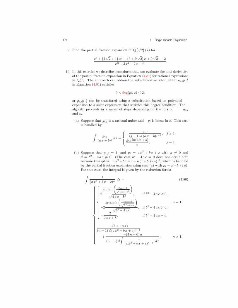
174 4. Single Variable Polynomials
9. Find the partial fraction expansion in Q√
2 (x) for
x4 + 2√
2 + 1 x2 + 5 + 9√
2 x + 9√
2 − 12
x3 + 3x2 − 2x− 6.
10. In this exercise we describe procedures that can evaluate the anti-derivativeof the partial fraction expansion in Equation (4.81) for rational expressionsin Q(x). The approach can obtain the anti-derivative when either gi,j/p
ji
in Equation (4.81) satisfies
0 < deg(pi, x) ≤ 2,
or gi,j/pji can be transformed using a substitution based on polynomial
expansion to a similar expression that satisfies this degree condition. Thealgorithm proceeds in a number of steps depending on the forms of gi,j
and pi.
(a) Suppose that gi,j is a rational number and pi is linear in x. This caseis handled by
gi,j
(ax + b)jdx =
− gi,j
(j − 1) a (a x + b)j−1, j > 1,
gi,j ln(ax + b)
a, j = 1.
(b) Suppose that gi,j = 1, and pi = a x2 + b x + c with a �= 0 andd = b2 − 4 a c �= 0. (The case b2 − 4 a c = 0 does not occur herebecause this implies a x2 + b x+ c = a (x+ b/(2a))2, which is handledby the partial fraction expansion using case (a) with pi = x+ b/(2 a).For this case, the integral is given by the reduction formula
1
(ax2 + b x + c)ndx = (4.86)
2
arctan 2 a x+b√4 a c−b2√
4 a c− b2, if b2 − 4 a c < 0,
−2
arctanh 2 a x+b√b2−4 a c√
b2 − 4 a c, if b2 − 4 a c > 0,
− 2
2a x + b, if b2 − 4 a c = 0,
n = 1,
−(b + 2 ax)
(n− 1) d (ax2 + b x + c)n−1
+−(4n− 6) a
(n− 1) d1
(ax2 + b x + c)n−1dx
, n > 1.
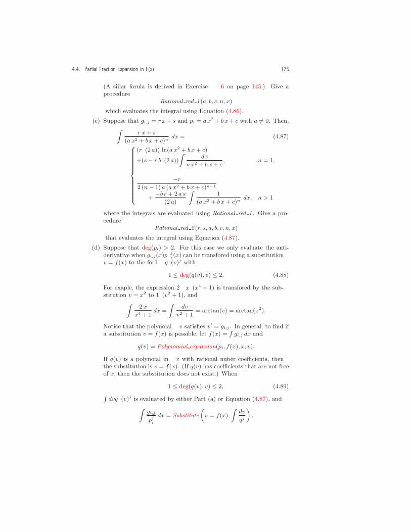
4.4. Partial Fraction Expansion in F(x) 175
(A similar formula is derived in Exercise 6 on page 143.) Give aprocedure
Rational red 1 (a, b, c, n, x)
which evaluates the integral using Equation (4.86).
(c) Suppose that gi,j = r x + s and pi = ax2 + b x + c with a �= 0. Then,
r x + s
(a x2 + b x + c)ndx = (4.87)
(r/(2 a)) ln(ax2 + b x + c)
+(s− r b/(2 a))dx
ax2 + b x + c, n = 1,
−r
2 (n− 1) a (a x2 + b x + c)n−1
+−b r + 2 a s
(2 a)
1
(a x2 + b x + c)ndx, n > 1
where the integrals are evaluated using Rational red 1 . Give a pro-cedure
Rational red 2 (r, s, a, b, c, n, x)
that evaluates the integral using Equation (4.87).
(d) Suppose that deg(pi) > 2. For this case we only evaluate the anti-derivative when gi,j(x)/pj
i (x) can be transformed using a substitutionv = f(x) to the form 1/q(v)j with
1 ≤ deg(q(v), v) ≤ 2. (4.88)
For example, the expression 2x/(x4 + 1) is transformed by the sub-stitution v = x2 to 1/(v2 + 1), and
2 x
x4 + 1dx =
dv
v2 + 1= arctan(v) = arctan(x2).
Notice that the polynomial v satisfies v′ = gi,j . In general, to find ifa substitution v = f(x) is possible, let f(x) = gi,j dx and
q(v) = Polynomial expansion(pi, f(x), x, v).
If q(v) is a polynomial in v with rational number coefficients, thenthe substitution is v = f(x). (If q(v) has coefficients that are not freeof x, then the substitution does not exist.) When
1 ≤ deg(q(v), v) ≤ 2, (4.89)
dv/q(v)j is evaluated by either Part (a) or Equation (4.87), and
gi,j
pji
dx = Substitute v = f(x),dv
qj.

176 4. Single Variable Polynomials
If deg(q(v), v) > 2, the anti-derivative is not evaluated by the tech-niques described here. Give a procedure
Rational red 3 (g, p, j, x)
that evaluates the anti-derivative of g/pj by
i. integrating g,
ii. obtaining the polynomial expansion with Polynomial expansion,
iii. checking if the substitution is possible, and
iv. evaluating the anti-derivative when the degree condition (4.89)is satisfied.
If the anti-derivative cannot be evaluated with this approach, returnthe global symbol Fail.
(e) Give a procedureRational red 4 (g, p, j, x)
that evaluates the anti-derivative of g/pj by evaluating the degreesof g and p and applying one of the cases (a), (b), (c), or (d). If theanti-derivative cannot be evaluated using these techniques, return theglobal symbol Fail.
(f) Let f be an algebraic expression. Give a procedure
Rational integrate(f, x)
that checks if f is a rational expression in Q(x) and when this is soevaluates f dx using the approach described in this exercise. If fdoes not have the proper form or if f dx cannot be evaluated usingthese techniques, return the global symbol Fail.
11. Give a procedureNumerical part frac(r)
that expresses a rational number 0 ≤ r < 1 in terms of rational numberswith prime denominators. For example, r = 1/6 = 1/2−1/3. To bypass theautomatic simplification of rational number expressions, use the functionrepresentations described in Figure 2.6 on page 39.
Use the ifactor operator in Maple and MuPAD and the FactorInteger
operator in Mathematica to obtain the prime factorization of the denom-inator of r. (Implementation: Maple (mws), Mathematica (nb), MuPAD(mnb).)
Further Reading
4.2 Greatest Common Divisors. See Akritas [2], Brown and Traub [16],Davenport et al. [29], Geddes et al. [39], Knuth [55], Yap [105], Mignotte [66],

4.4. Partial Fraction Expansion in F(x) 177
von zur Gathen and Gerhard [96], and Zippel [108] for modern approaches ingreatest common divisor calculation.
4.3 Computations in Algebraic Number Fields. See Buchberger et al.[17] and Smedley [91] for discussions of computations in algebraic number fields.Landau [60] describes an algorithm for denesting radicals based on Galois theory.
4.4 Partial Fraction Expansion. von zur Gathen and Gerhard [96] discuss
partial fraction expansion.


5
Polynomial Decomposition
A polynomial u(x) is called a composite polynomial if there are polyno-mials v(w) and w(x), both with degree greater than one, such that u isrepresented by the functional composition u(x) = v(w(x)). The compos-ite expression v(w(x)) is also called a decomposition of u in terms of thecomponents v(w) and w(x), and the process for finding v and w is calleddecomposing a polynomial. For example,
u(x) = x4 − 5 x2 + 6 (5.1)
is a composite polynomial with decomposition given by
v(w) = w2 − 5w + 6, w(x) = x2.
Decomposition plays an important role in the solution of polynomialequations. For example, to solve
u(w(x)) = (x2)2 − 5 (x2) + 6 = 0,
first solve the equation for w(x) = x2 to obtain x2 = 2, 3, and then solvethese equations to obtain x = ±√2,±√3. Most computer algebra systemsapply decomposition as part of the solution of polynomial equations.
It is easy to recognize that u(x) in Equation (5.1) is a composite poly-nomial. With more involved examples, however, a decomposition may notbe apparent or even possible. For example,
u(x) = x4 + 4 x3 + 3 x2 − 2 x+ 3 (5.2)
179

180 5. Polynomial Decomposition
can be decomposed as
(x2 + 2 x+ 1)2 − 3 (x2 + 2 x+ 1) + 5, (5.3)
while u(x) + x cannot be decomposed at all.How can we determine if a polynomial can be decomposed? Surpris-
ingly, there are some simple algorithms that do the job. In Section 5.1 wedescribe the basic theoretical concepts of polynomial decomposition, and inSection 5.2 we describe an algorithm that either finds a decomposition foru(x) (if one exists) or determines that no such decomposition is possible.
5.1 Theoretical Background
In this chapter all polynomials u(x) are in Q[x]. First of all, it is conve-nient to simplify our notation. We denote a composite polynomial u(x) =v(w(x)) using the operator notation ◦ as
u = v ◦ w,and to emphasize the dependence on a variable x, we represent the com-posite as
u(x) = (v ◦ w)(x).For example, the composite polynomial
u(x) = (x2 + 2 x+ 1)2 − 3 (x2 + 2 x+ 1) + 5,
is expressed as
u(x) = (w2 − 3w + 5) ◦ (x2 + 2 x+ 1). (5.4)
It also simplifies matters if we use the same variable name x to describe allpolynomial formulas. With this convention, Equation (5.4) becomes
u(x) = (x2 − 3 x+ 5) ◦ (x2 + 2 x+ 1).
Using the ◦ notation we can also represent more complex composite ex-pressions such as
f(x) = (u ◦ v ◦ w)(x) = u(v(w(x))).
Actually, the composition symbol ◦ is nothing more than a shorthand no-tation for the Substitute operator
(v ◦ w)(x) = Substitute(v(x), x = w(x)).
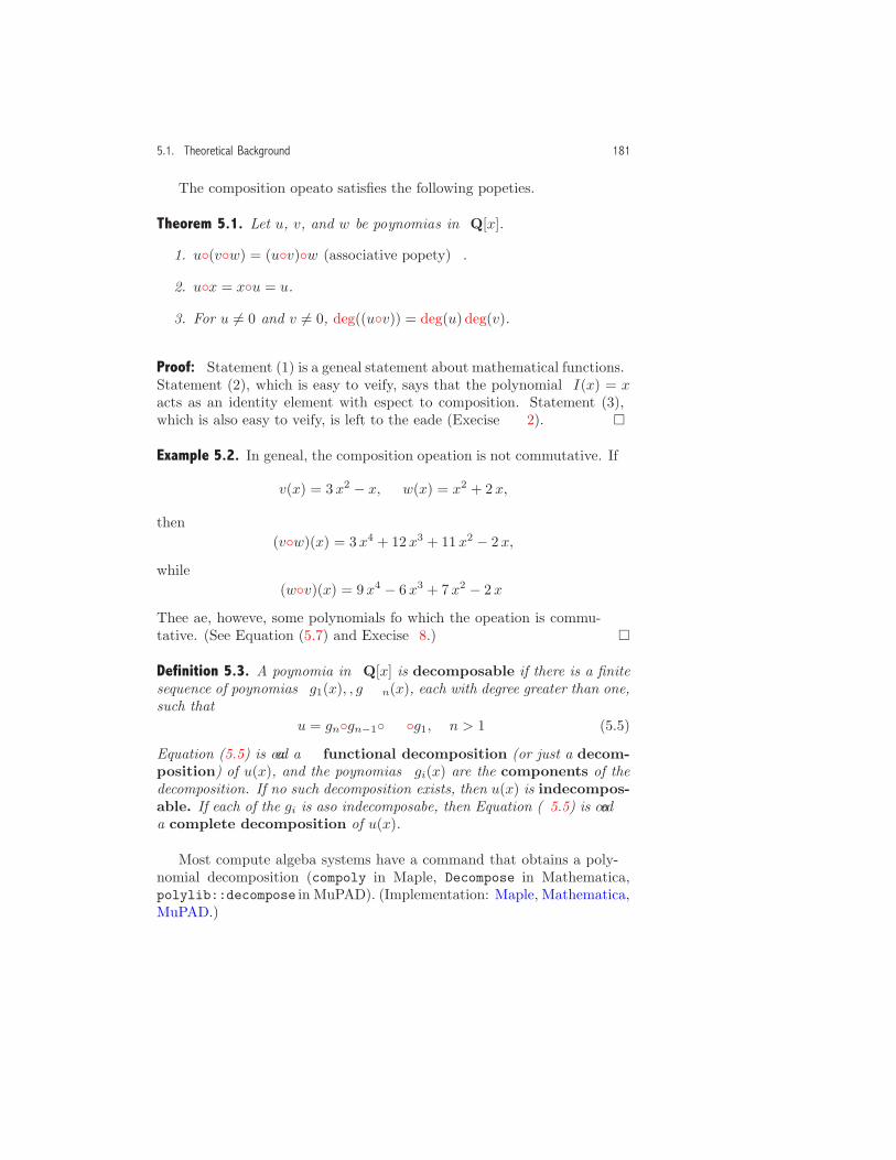
5.1. Theoretical Background 181
The composition operator satisfies the following properties.
Theorem 5.1. Let u, v, and w be polynomials in Q[x].
1. u◦(v◦w) = (u◦v)◦w (associative property).
2. u◦x = x◦u = u.
3. For u �= 0 and v �= 0, deg((u◦v)) = deg(u) deg(v).
Proof: Statement (1) is a general statement about mathematical functions.Statement (2), which is easy to verify, says that the polynomial I(x) = xacts as an identity element with respect to composition. Statement (3),which is also easy to verify, is left to the reader (Exercise 2). �
Example 5.2. In general, the composition operation is not commutative. If
v(x) = 3 x2 − x, w(x) = x2 + 2 x,
then(v◦w)(x) = 3 x4 + 12 x3 + 11 x2 − 2 x,
while(w◦v)(x) = 9 x4 − 6 x3 + 7 x2 − 2 x.
There are, however, some polynomials for which the operation is commu-tative. (See Equation (5.7) and Exercise 8.) �
Definition 5.3. A polynomial in Q[x] is decomposable if there is a finitesequence of polynomials g1(x), . . . , gn(x), each with degree greater than one,such that
u = gn◦gn−1◦ . . . ◦g1, n > 1. (5.5)
Equation (5.5) is called a functional decomposition (or just a decom-position) of u(x), and the polynomials gi(x) are the components of thedecomposition. If no such decomposition exists, then u(x) is indecompos-able. If each of the gi is also indecomposable, then Equation (5.5) is calleda complete decomposition of u(x).
Most computer algebra systems have a command that obtains a poly-nomial decomposition (compoly in Maple, Decompose in Mathematica,polylib::decompose in MuPAD). (Implementation: Maple, Mathematica,MuPAD.)

182 5. Polynomial Decomposition
The definition requires that the decomposition be non-trivial in thesense that all components gi must have degree greater than one. Thismeans
4 x2 + 18 x+ 22 = (2 x+ 3)2 + 3 (2 x+ 3) + 4is not a decomposition because 2 x+ 3 has degree one.
Example 5.4. The following polynomial has a decomposition with threecomponents:
u(x) = x8 + 4 x7 + 10 x6 + 16 x5 + 29 x4 + 36 x3 + 40 x2 + 24 x+ 39
=((x2 + x)2 + 2 (x2 + x)
)2 + 12((x2 + x)2 + 2 (x2 + x)
)+ 39
= (x2 + 12 x+ 39)◦(x2 + 2 x)◦(x2 + x).
Since none of the components can be decomposed, the decomposition iscomplete (Exercise 3). �
Example 5.5. A complete decomposition of a polynomial is not unique.For example, here are two different decompositions of a polynomial:
u(x) = x6 + 2 x4 + x2 + 1= (x3 + 2 x2 + x+ 1)◦(x2) (5.6)= (x3 − x2 + 1)◦(x2 + 1). �
In fact, any polynomial that can be decomposed has infinitely manydecompositions. This fact is based on the observation that the two linearpolynomials f(x) = mx+b and g(x) = x/m−b/m are inverses with respectto composition because they satisfy the property
(f◦g)(x) = (g◦f)(x) = x. (5.7)
Therefore, if u has a decomposition u = v◦w, another decomposition isobtained (using Theorem 5.1) in the following way:
u = v◦w = v◦x◦w = v◦(f◦g)◦w = (v◦f)◦(g◦w). (5.8)
For Equation (5.6), with f = x − 1, g = x+ 1, this construction takes theform:
u(x) = x6 + 2 x4 + x2 + 1= (x3 + 2 x2 + x+ 1)◦x2
= (x3 + 2 x2 + x+ 1)◦x◦x2 (5.9)= (x3 + 2 x2 + x+ 1)◦((x− 1)◦(x+ 1)
)◦x2
=((x3 + 2 x2 + x+ 1)◦(x− 1)
)◦((x+ 1)◦x2)
= (x3 − x2 + 1)◦(x2 + 1).
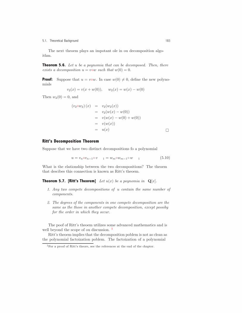
5.1. Theoretical Background 183
The next theorem plays an important role in our decomposition algo-rithm.
Theorem 5.6. Let u be a polynomial that can be decomposed. Then, thereexists a decomposition u = v◦w such that w(0) = 0.
Proof: Suppose that u = v◦w. In case w(0) �= 0, define the new polyno-mials
v2(x) = v(x+ w(0)), w2(x) = w(x) − w(0).
Then w2(0) = 0, and
(v2◦w2) (x) = v2(w2(x))= v2(w(x) − w(0))= v(w(x) − w(0) + w(0))= v(w(x))= u(x). �
Ritt’s Decomposition Theorem
Suppose that we have two distinct decompositions for a polynomial
u = vn◦vn−1◦ . . . v1 = wm◦wm−1◦ . . . w1. (5.10)
What is the relationship between the two decompositions? The theoremthat describes this connection is known as Ritt’s theorem.
Theorem 5.7. [Ritt’s Theorem] Let u(x) be a polynomial in Q[x].
1. Any two complete decompositions of u contain the same number ofcomponents.
2. The degrees of the components in one complete decomposition are thesame as the those in another complete decomposition, except possiblyfor the order in which they occur.
The proof of Ritt’s theorem utilizes some advanced mathematics and iswell beyond the scope of our discussion.1
Ritt’s theorem implies that the decomposition problem is not as clean asthe polynomial factorization problem. The factorization of a polynomial
1For a proof of Ritt’s theorem, see the references at the end of the chapter.

184 5. Polynomial Decomposition
into irrreducible factors is unique up to the order of the factors (Theo-rem 4.38, page 138). On the other hand, two complete decompositions ofa polynomial can look quite different. For example,
x6 + 2 x4 + x2 + 1 = (x3 + 2 x2 + x+ 1)◦(x2) (5.11)= (x2 + 1)◦(x3 + x).
Notice that each of these complete decompositions contains two polynomi-als, one with degree two and one with degree three, but the degrees appearin opposite order.
We have seen that one way two decompositions of a polynomial candiffer is through the application of linear polynomials and their inversesas is done in Equation (5.8). In fact, in some cases, it is possible to gofrom one decomposition to another by simply inserting linear polynomialsand their inverses at appropriate places in the first decomposition (seeEquation (5.9)). When this happens, the two decompositions are calledequivalent decompositions. However, the situation can be more complex.For example, the two decompositions in Equation (5.11) are not equivalentin this sense because it is impossible to change the order of the degreesin a decomposition by simply inserting a linear polynomial and its inverse(Exercise 4).
The relationship between different decompositions of a polynomial canbe described in more detail than we have done in this brief discussion.However, it is not necessary to understand these relationships to describea decomposition algorithm, and because the algorithm is our primary goal,we will not pursue this matter further. The reader who is interested inpursuing these questions should consult the references at the end of thechapter.
Sufficiency of Rational Decompositions
We conclude this section with an important theoretical point. Supposethat u is a polynomial in Q[x] that is indecomposable if we require thatthe components are also in Q[x]. Might it be possible to decompose u interms of polynomials with coefficients in a larger number field? After all,a polynomial’s irrreducible factorization depends on the coefficient field.Could the same thing happen for decompositions? Fortunately, for poly-nomial decomposition the answer is no.
Theorem 5.8. Suppose that u is a polynomial in Q[x] that has a decom-position u = v◦w. Then, u has an equivalent decomposition in terms ofpolynomials with rational number coefficients.

5.1. Theoretical Background 185
Proof: Suppose that u = v◦w. By Theorem 5.6, there is an equivalentdecomposition with w(0) = 0, so we assume that w satisfies this property.In a similar way, we can also find an equivalent decomposition so that w isa monic polynomial (Exercise 11(a)); therefore, we assume that w satisfiesthis property as well. We show that if u has rational coefficients and ifw satisfies these two properties, then both w and v must have rationalcoefficients as well.
Letu = um xm + um−1 x
m−1 + · · ·+ u1 x+ u0,
v = vn xn + vn−1 x
n−1 + · · ·+ v1 x+ v0, n > 1,
w = xp + wp−1 xp−1 + · · ·+ w1 x, p > 1, (5.12)
where the degrees of the polynomials satisfy the relation m = n p. (Noticethat w in Equation (5.12) is monic and w(0) = 0.) Then
u = v◦w= vn (xp + wp−1 x
p−1 + · · ·+ w1 x)n
+vn−1 (xp + wp−1 xp−1 + · · ·+ w1 x)n−1 (5.13)
+ · · ·+ v1 (xp + wp−1 xp−1 + · · ·+ w1 x) + v0.
In this representation, vn is the coefficient of xnp, and since np = m =deg(u), we have
vn = um (5.14)
which shows that vn is a rational number. In addition, the largest powerof x that is contributed by the second term of the representation (5.13) isxp (n−1), and so all of the powers
xp n, xp n−1, . . . , xp (n−1)+1
come from the first term
vn (xp + wp−1xp−1 + · · ·+ w1x)n. (5.15)
By examining the form of the coefficients in the expression (5.15), we willshow that all the coefficients of w are rational.
For example, let’s look at the coefficient of xp n−1. Expanding theexpression (5.15) with the binomial theorem, we have
vn(xp +
(wp−1 x
p−1 + · · ·+ w1 x))n
= vn
((xp)n + n (xp)n−1 (
wp−1 xp−1 + wp−2 x
p−2 + · · ·+ w1 x)
+n (n− 1)
2(xp)n−2 (
wp−1 xp−1 + wp−2 x
p−2 + · · ·+ w1 x)2
+ · · ·).
(5.16)

186 5. Polynomial Decomposition
Observe that the largest power of x that is contributed by the second termin Equation (5.16) is
xp (n−1)+(p−1) = xp n−1,
and the largest power contributed by the third term is
xp (n−2)+2 (p−1) = xp n−2.
From these observations, the coefficient of xp n−1 in Equation (5.16) isvn nwp−1, and since n p− 1 = m− 1, we have from Equation (5.13)
um−1 = vn nwp−1.
Therefore, since um−1 and vn are both rational, wp−1 is rational as well.Let’s consider next the coefficient of xpn−2 in Equation (5.16). This
term is obtained with
vn
(nxp (n−1) wp−2 x
p−2 +n (n− 1)
2xp (n−2) w2
p−1 x2 (p−1)
)
= vn
(nwp−2 +
n (n− 1)2
w2p−1
)xp n−2.
Therefore, since n p− 2 = m− 2, we have from Equation (5.13)
um−2 = vn
(nwp−2 +
n (n− 1)2
w2p−1
),
and since um−2, vn, and wp−1 are rational, wp−2 is also rational. Contin-uing in this fashion, we show that all the coefficients of w are rational.
We can also show that the coefficients of v are rational by comparingcoefficients in Equation (5.13). We have shown above that vn is rational (seeEquation (5.14)), and to show that vn−1 is rational, consider the coefficientsof xp (n−1). From Equation (5.13), we have
up (n−1) = vn r + vn−1,
where r is obtained by combining coefficients of xp (n−1) from the term
(xp + wp−1 xp−1 + · · ·+ w1 x)n.
Since, all the coefficients of w are rational, r is rational, and since up(n−1)
and vn are rational, vn−1 is rational as well. In a similar way, by comparingcoefficients of xp (n−2), we can show that vn−2 is rational. Continuing inthis fashion, we can show that all of the coefficients of v are rational. �

5.1. Theoretical Background 187
Exercises1. For the polynomial in Equation (5.2), solve the equation u(x) = 0 with the
help of polynomial decomposition.
2. Prove Theorem 5.1(3).
3. Explain why a polynomial of degree two or degree three cannot be decom-posed.
4. Explain why the order of the degrees in a decomposition of a polynomialu(x) cannot be changed by the insertion of a linear polynomial and itsinverse between two components.
5. Is every indecomposable polynomial irrreducible? Is every irrreduciblepolynomial indecomposable?
6. Find six distinct decompositions of u(x) = x30 such that the powers of thecomponents appear in different orders.
7. Find two different decompositions for the polynomial u = x4 + 2x3 +x2. Hint: there is a decomposition with one component x2. Do not usecomputer algebra software for this problem.
8. The Chebyshev polynomial Tn(x) of degree n is defined (for −1 ≤ x ≤ 1)by the trigonometric relations
Tn(x) = cos(n θ), x = cos(θ).
For example, T0(x) = cos(0) = 1 and T1(x) = cos(θ) = x.
(a) Show that T2(x) = 2x2 − 1.
(b) Derive the recurrence relation
Tn+1(x) = 2xTn(x) − Tn−1(x).
Hint: Use the identity cos(a + b) + cos(a− b) = 2 cos(a) cos(b).
(c) Show that Tm n = Tm◦Tn.
(d) Show that Tn◦Tm = Tm◦Tn. In other words, the polynomials Tn andTm commute under composition.
9. Consider the two monic polynomials u = x2 + b x+ c and v = x2 + e x+ f .Show that if u◦v = v◦u, then u = v. (This implies that two distinctquadratic polynomials cannot commute with respect to composition.)
10. Consider the following four polynomials:
u1 = 2x2 + 3x + 4, v1 = x2 − 5,
u2 = 8x2 + 30 x + 31, v2 =x2
2− 4.
(a) Show that u1◦v1 = u2◦v2.
188 5. Polynomial Decomposition
(b) Find polynomials f = mx+b and g = x/m−b/m such that u1◦f = u2
and g◦v1 = v2.
11. Suppose that u has a complete decomposition
u = gp◦gp−1◦ · · · ◦g1.
(a) Show that it is possible to modify the decomposition so that all ofthe components except gp are monic.
(b) Show that it is possible to modify the decomposition so that the onlycomponent that has a constant term is gp.
12. In this exercise we describe a collection of polynomials that illustrates thesecond statement in Ritt’s Theorem 5.7 (page 183). Let g(x) be a non-zeropolynomial, and consider the polynomials
u(x) = xn, v(x) = xr g(xn), w(x) = xr g(x)n.
(a) Show that deg(v, x) = deg(w, x) = r + deg(g, x)n.
(b) Show that u◦v = w◦u.
(c) Show that, if n and r+ deg(g, x)n are prime numbers, then u, v, andw are indecomposable.
This implies, if n and r+ deg(g, x)n are distinct as well as prime, that u◦vand v◦w are two distinct complete decompositions of the same polynomialwith degrees that occur in opposite order. For example, for n = 3, r = 2,and g(x) = x3 − 1, we have v = x11 − x2, w = x11 − 3 x8 + 3 x5 − x2, andu◦v = w◦u = x33 − 3x24 + 3 x15 − x6.
13. The polynomialu = x4−10x3 + 27 x2−10x + 3
can be decomposed as
u = 2x2 +2√
6
3+ 2
√2 x +
10
3+
2√
3
3◦
√2
2x2 − 5
√2
2x−
√6
6.
Find an equivalent decomposition that involves polynomials with rationalcoefficients.
5.2 A Decomposition Algorithm
In this section we describe an algorithm that finds the complete decom-position of a polynomial u(x) (if it exists) or determines that no suchdecomposition is possible. We begin, however, by looking at the simplerproblem of finding a two-level decomposition u = v◦w. In some cases, itwill be possible to decompose v or w.

5.2. A Decomposition Algorithm 189
Let’s assume that u = v◦w, and let
u(x) = umxm + um−1x
m−1 + · · ·+ u1x+ u0,
v(x) = vnxn + vn−1x
n−1 + · · ·+ v1x+ v0.
The algorithm is based on the properties of a decomposition that are de-scribed in Theorems 5.9 and 5.10.
Theorem 5.9. Let u be a polynomial in Q[x] that can be decomposed. Then,there is a decomposition u = v◦w such that w satisfies the following prop-erties.
1. 1 < deg(w, x) < deg(u, x).
2. deg(w, x) | deg(u, x).3. w(0) = 0.
4. w(x)|(u(x)− u0).
Proof: Property (1), which follows from Theorem 5.1(3), is just a re-statement of the property that both v and w must have degree greaterthan 1. Property (2) also follows from Theorem 5.1(3). Property (3) is arestatement of Theorem 5.6.
To show property (4), we have, using property (3),
u0 = u(0) = v(w(0)) = v(0) = v0.
Therefore,
u(x)− u0 = u(x)− v0
= vnw(x)n + vn−1w(x)n−1 + · · ·+ v1w(x),
and since w(x) divides each term in the sum, it also divides u(x)− u0. �
The property w(0) = 0 is a sufficient condition to guarantee that
w(x)|(u(x)− u0)
but it is not a necessary condition. There can be other divisors of u(x)−u0
that don’t satisfy this condition but lead to a decomposition (see Exam-ple 5.11).
Although we don’t know which divisors of u(x) − u0 lead to a decom-position, we do know that there is a decomposition v(x)◦w(x) for which

190 5. Polynomial Decomposition
w(x) is one of these divisors. The next theorem gives a way to computev(x) and provides a test that determines whether or not some trial divisorw(x) of u(x)− u0 leads to a decomposition.
Theorem 5.10. Suppose that a polynomial u in Q[x] can be decomposed asu = v◦w. Then v is given by the polynomial expansion of u in terms of w,and this expansion has coefficients that are free of x.
Proof: Since u = v◦w,u(x) = vn w(x)n + vn−1 w(x)n−1 + · · ·+ v1 w(x) + v0 (5.17)
where the coefficients vi are rational numbers. But the representation(5.17) is just the (unique) polynomial expansion u in terms of w (seeTheorem 4.13 on page 118). In general, the coefficients in a polynomialexpansion can be polynomials in x, but, in this case, the vi are rationalnumbers and therefore free of x. �
The two previous theorems suggest the following approach to find adecomposition for u(x). First, find the set of distinct polynomial divisorsof u(x)−u0. These divisors are found by first finding all irrreducible (non-constant) factors of u(x) − u0 and then forming all possible products ofthese factors. In this context, multiplication of a divisor w by a rationalnumber c is not another distinct divisor, and so, it is sufficient to consideronly monic divisors. For example, the set of distinct polynomial divisorsof 3 (x− 1) (x− 2)2 is (in factored form)
S ={x− 1, x− 2, (x − 2)2, (x− 1) (x− 2), (x− 1) (x− 2)2
}.
Each divisor that satisfies properties (1), (2), and (4) of Theorem 5.9 is apotential candidate for w(x).
Next, for each such candidate w(x) in S, form the polynomial expan-sion (5.17). If all the coefficients vi are free of x, then v and w give adecomposition of u. On the other hand, if none of the divisors in S leadsto an expansion with this property, then u is indecomposable.
Example 5.11. Consider the polynomial u(x) = x6 + 6 x4 + 3 x3 + 9 x2 +9 x+ 5. Since u(x)− 5 can be factored as
u(x)− 5 = x (x2 + 3) (x3 + 3x+ 3),
the divisor set is
S ={x, x2 + 3, x(x2 + 3), x3 + 3 x+ 3, x (x3 + 3 x+ 3),
(x2 + 3) (x3 + 3 x+ 3), x (x2 + 3) (x3 + 3 x+ 3)}. (5.18)

5.2. A Decomposition Algorithm 191
However, the only polynomial that satisfies all the properties of Theo-rem 5.9 is w(x) = x3 +3 x. To see if this expression gives a decomposition,we find the polynomial expansion2 of u in terms of w:
v(t) = Polynomial expansion(u, w, x, t)→ t2 + 3 t+ 5.
Since all of the coefficients of v(t) are free of x, we have the decomposition
u = v(x)◦w(x) = (x2 + 3 x+ 5)◦(x3 + 3 x).
There are two other divisors in (5.18) that do not satisfy Theorem 5.9(3) but do satisfy Parts (1), (2), and (4):
x2 + 3, x3 + 3 x+ 3.
For these cases, the polynomial expansions are
w(x) = x3 + 3 x+ 3, v(t) = t2 − 3 t+ 5, (5.19)w(x) = x2 + 3, v(t) = t3 − 3 t2 + 3 x t+ 5. (5.20)
Since v(t) in (5.19) is free of x, we have another decomposition
u = v(x)◦w(x) = (x2 − 3 x+ 5)◦(x3 + 3 x+ 3)
even though w(0) �= 0. On the other hand, since v(t) in (5.20) is not freeof x, we do not obtain an expansion with w(x) = x2 + 3. �
Example 5.12. Consider the polynomial u(x) = x4 + x3 + 3. Since
u(x)− 3 = x3 (x + 1),
the divisor set is
S ={x, x+ 1, x2, x2 + x, x3, x3 + x2, x4 + x3
}.
The only divisors that satisfy all the properties of Theorem 5.9 are w1(x) =x2+x and w2(x) = x2. The polynomial expansion of u in terms of w1(x) is
3− x t+ t2
and the expansion in terms of w2(x) is
3 + x t+ t2.
2The Polynomial expansion operator is given in Figure 4.2 on page 122.

192 5. Polynomial Decomposition
Procedure Poly decomp 2 (u, x);Input
u : a polynomial in Q[x];x : a symbol;
OutputEither a decomposition [v, w] or u if no decomposition exists;
Local Variables U, S, i, w, v;Global t;Begin
1 U := u− Coefficient gpe(u, x, 0);2 S := Polynomial divisors(U, x);3 i := 1;4 while i ≤ Number of operands(S) do5 w := Operand(S, i);6 if Degree gpe(w, x) �= Degree gpe(u, x) and Degree gpe(w, x) > 1
and Irem(Degree gpe(u, x), Degree gpe(w, x)) = 0 then7 v := Polynomial expansion(u,w, x, t);8 if Free of(v, x) then9 Return[(Substitute(v, t = x), w]);10 i := i + 1;11 Return(u)
End
Figure 5.1. An MPL procedure for a two-level polynomial decomposition. (Im-plementation: Maple (txt), Mathematica (txt), MuPAD (txt).)
In both cases, the expansion has a coefficient that depends on x, and so,u(x) cannot be decomposed in terms of these polynomials. Therefore, u(x)cannot be decomposed. �
A procedure for the decomposition process is shown in Figure 5.1. Ifu is decomposable, the procedure returns a list [v, w] that contains thepolynomials that make up a two-level decomposition, and if u is not de-composable, then the procedure returns u. The global symbol t is a mathe-matical symbol that is used in line 7 as an auxiliary variable in the operatorPolynomial expansion. We have used a global symbol to avoid using a localvariable that would not be assigned before it was used (see page 3).
At line 2, the operator Polynomial divisors is used to obtain the divi-sors3 of u − u0. At line 7, the operator Polynomial expansion returns apolynomial in terms of the fourth input parameter t with coefficients that
3The Polynomial divisors procedure is described in Exercise 12 on page 125. Thefactorization of u − u0 is obtained by the factor operator of a CAS in this procedure.

5.2. A Decomposition Algorithm 193
may depend on x. We check for this possibility by applying the Free ofoperator to the entire polynomial (line 8). If the while loop (lines 4–10)does not find a decomposition, the polynomial u cannot be decomposed.In this case, the algorithm simply returns u (line 11).
Notice that the algorithm does not check the condition w(0) = 0 andmay return a decomposition without this property.
The Complete Decomposition Algorithm
Next, we describe an algorithm that finds a complete decomposition foru. The algorithm either finds a sequence of indecomposable polynomialsg1, g2, . . . , gp (with p > 1) such that
u = gp◦gp−1◦ · · · ◦g1
or determines that u is indecomposable. The general idea is to build upthe decomposition, one component at a time, taking care not to miss anyintermediate components. We show below that it is possible to arrangethings so that each of the partial compositions
gi◦gi−1◦ · · · ◦g1, 1 ≤ i < p,
is a divisor of u−u0 where the components gi are obtained with polynomialexpansions (Theorems 5.13 and 5.14). We insure that each gi is indecom-posable by applying a minimal degree condition to the divisors of u − u0
(Theorem 5.15).Let’s see how to find the component gi (for i < p) assuming that the
components g1, g2, . . . , gi−1 have already been found. (The last componentgp is computed in a different way.) To simplify the notation, let
u = gp◦gp−1◦ · · · ◦gi+1◦gi◦gi−1◦ · · · ◦g1
= R◦gi◦C,where
C = gi−1◦ · · · ◦g1 (5.21)
is the decomposition so far and
R = gp◦gp−1◦ · · · ◦gi+1 (5.22)
is the decomposition that remains to be found after gi has been found. (Fori = 1 we initialize C to x.) Since i < p, we can assume that deg(R, x) > 0.
Theorem 5.13. Let u be a polynomial in Q[x] that can be decomposed as
u = R◦gi◦C.Then, for i < p, it is possible to choose gi with the following properties:

194 5. Polynomial Decomposition
1. deg(C, x) < deg(gi◦C, x) < deg(u, x).
2. deg(gi◦C, x) | deg(u, x).
3. (gi◦C)(0) = 0.
4. (gi◦C)(x)| (u(x)− u0).
Proof: The proof of this theorem is similar to the proof for Theorem 5.9(Exercise 5). �
The theorem implies that we can find gi◦C by examining the divisorsof u(x) − u0. Notice in this case that we do not get gi directly as somedivisor of u − u0, but instead obtain the composite expression gi◦C. Thisis consistent with what was done in the two-level algorithm because whencomputing g1, C is initialized to x and we get g1 directly.
The next theorem gives a way to compute gi from gi◦C and provides away to tell if some trial divisor of u− u0 contributes to the decomposition.
Theorem 5.14. Suppose that u in Q[x] can be decomposed as u = R◦gi◦C.
1. The polynomial R is found by computing the polynomial expansion ofu in terms of gi◦C, and this expansion has coefficients that are freeof x.
2. The polynomial gi is found by computing the polynomial expansion ofgi◦C in terms of C, and this expansion has coefficients that are freeof x.
Proof: To verify (1), let
R = rs xs + rs−1 x
s−1 + · · ·+ r0.
Observe that
u = R◦gi◦C = rs (gi(C))s + rs−1 (gi(C))s−1 + · · ·+ r0,
which is just the unique polynomial expansion of u in terms of gi(C).Since the coefficients rs, rs−1, . . . , r0 are rational numbers, they are free ofx. Although statement (1) is similar to Theorem 5.10 in the two-level case,we shall see that R only becomes part of the decomposition when findingthe final component gp. For the other components gi, i < p, we need onlycheck that the coefficients of R are free of x.
5.2. A Decomposition Algorithm 195
To verify (2), let
gi(x) = ap xp + ap−1 x
p−1 + · · ·+ a1 x+ a0.
Observe that
(gi◦C)(x) = ap (C(x))p + ap−1 (C(x))p−1 + · · ·+ a1 C(x) + a0, (5.23)
which is just the unique polynomial expansion of gi◦C in terms of C. Inorder for gi to be a component, its coefficients must be rational numbersand hence free of x. �
The next theorem provides a way to choose gi◦C so that gi is indecom-posable.
Theorem 5.15. Let u = R◦gi◦C, and suppose that gi◦C is the divisor ofu(x) − u0 of minimal degree that satisfies the conditions in Theorem 5.13and Theorem 5.14. Then, gi is indecomposable.
Proof: If gi were decomposable, then we can show that gi◦C does notsatisfy the minimal degree condition. To see why, suppose that gi is de-composable as
gi = v◦wwith deg(v, x) > 1 and deg(w, x) > 1. (This implies that deg(w, x) <deg(gi, x).) Then
u = R◦gi◦C = R◦v◦w◦C= (R◦v)◦(w◦C).
By an argument similar to the one in the proof of Theorem 5.9, we canassume that (w◦C)(0) = 0, and therefore w◦C is a divisor of u− u0. Since
deg(w◦C, x) = deg(w, x) deg(C, x)< deg(gi, x) deg(C, x)= deg(gi◦C, x),
gi◦C does not satisfy the minimal degree condition. Therefore gi must beindecomposable. �
The above theorems suggest the following approach for finding a com-plete decomposition of u(x). First, find all the divisors of u − u0. To findg1, initialize C to x, and find a divisor w of u− u0 of smallest degree that

196 5. Polynomial Decomposition
satisfies the conditions in Theorems 5.13 and 5.14. Since C = x, we imme-diately have g1 = w as was done in the two-level case.4 If no such divisorw exists, u is indecomposable.
To compute gi (1 < i < p), let C = gi−1◦ · · · ◦g1 be the decompositionso far, and let w be a divisor of u− u0 of minimal degree that satisfies theconditions in Theorems 5.13 and 5.14. In this case, we find gi using thepolynomial expansion of w in terms of C as is done in Equation (5.23).If no such divisor w exists, then C includes the first p − 1 components inthe decomposition and we need only compute the last component gp. Thiscomponent can be found by computing the polynomial expansion of u interms of C. It is not difficult to show that gp computed in this way isindecomposable (Exercise 6).
Example 5.16. Consider the polynomial
u := x8 + 4 x7 + 6 x6 + 4x5 + 3x4 + 4x3 + 2 x2 + 1.
The polynomial u− 1 can be factored as
u− 1 = x2 (x4 + 2 x3 + x2 + 2) (x+ 1)2.
Although there are 17 divisors of u − 1, the degree requirements of Theo-rem 5.13 eliminate all but five of them:
x2, x2 + x, x2 + 2x+ 1, x4 + 2x3 + x2, x4 + 2x3 + x2 + 2. (5.24)
To compute g1, let C = x, and first consider the three divisors of degreetwo in (5.24). There are three possibilities for g1◦C:
g1◦C = x2, R = t4 + (4 x+ 6) t3 + (4 x+ 3) t2
+ 2 t+ 1, (5.25)g1◦C = x2 + x, R = t4 + 2 t2 + 1, (5.26)g1◦C = x2 + 2 x+ 1, R = t4 + (2−4 x) t3 + (−1−4 x) t2
+ (−2−4 x) t+ 1. (5.27)
Again, we have expressed the polynomial expansions for R in terms ofa variable t to clearly distinguish the coefficients that may depend on x.(When C = x, we have g1◦C = g1, and so we have not computed thepolynomial expansion of g1◦C in terms of C.) Since R in (5.26) is the onlyone with coefficients that are free of x, we choose
g1◦C = x2 + x,4For the sake of consistency, the algorithm finds g1 using polynomial expansion even
though it can be found directly.

5.2. A Decomposition Algorithm 197
and since C = x,g1 = x2 + x.
Now to choose g2, let C = g1 and observe there are two divisors withdegree four in (5.24), each of which is a candidate for g2◦C. Computingthe polynomial expansions in Theorem 5.14 for each of them, we obtain
g2◦C = x4 + 2x3 + x2, g2 = t2, (5.28)R = t2 + 2t+ 1, (5.29)
or
g2◦C = x4 + 2x3 + x2 + 2, g2 = t2 + 2, (5.30)R = t2 − 2t+ 1. (5.31)
In both cases, both g2 and R are free of x and so either divisor will con-tribute to the decomposition. Using Equation (5.28) (with x substitutedfor t), we have g2 = x2. Since there are no more divisors to consider, weobtain g3 by substituting x for t in R in Equation (5.29). Therefore, acomplete decomposition is
u = (x2 + 2x+ 1)◦(x2)◦(x2 + x). �
A procedure that obtains the complete decomposition of a polyno-mial in Q[x] is shown in Figure 5.2. The procedure returns either a list[gp, gp−1, . . . , g1] that represents the decomposition or u if the polynomialis indecomposable. The while loop (lines 5–14) examines the divisors ofU = u− u0 and tries to choose an appropriate one to build up the decom-position. At line 6, the Find min deg operator (Exercise 4) chooses a trialdivisor w of minimal degree from the set S, and the statement at line 8checks the degree requirements mentioned in Theorem 5.13. If w passesthese tests, the polynomial expansions referred to in Theorem 5.14 arecomputed (lines 9–10), and the conditions mentioned in this theorem arechecked in line 11. (Recall that the operator Polynomial expansion returnsa polynomial in terms of the fourth input parameter t with coefficientsthat may depend on x.) If both expansions are free of x, we have foundthe next component which is adjoined to the list decomposition (line 12).At line 13, C is assigned the value w in preparation for searching for thenext component.
At line 14, the polynomial expansion R is assigned to final component .At this point, R has been used only to check the validity of w for computingthe next component (line 11). However, when the next to last component(gp−1) is computed, the current value of R is the polynomial expansion of

198 5. Polynomial Decomposition
Procedure Complete poly decomp(u, x);Input
u : a polynomial in Q[x] ;x : a symbol;
OutputA decomposition [gp, gp−1, . . . , g1] or u if no decomposition exists;
Local VariablesU, S, decomposition , C,w, g,R,final component ;
Global t;Begin
1 U := u− Coefficient gpe(u, x, 0);2 S := Polynomial divisors(U, x);3 decomposition := [ ];4 C := x;5 while S �= ∅ do6 w := Find min deg(S, x);7 S := S − {w};8 if Degree gpe(C,x) < Degree gpe(w, x)
and Degree gpe(w, x) < Degree gpe(u, x)and Irem(Degree gpe(u, x),Degree gpe(w, x)) = 0 then
9 g := Polynomial expansion(w,C, x, t);10 R := Polynomial expansion(u,w, x, t);11 if Free of(g, x) andFree of(R, x) then12 decomposition := Adjoin(Substitute(g, t = x), decomposition);13 C := w;14 final component := R;15 if decomposition = [ ] then16 Return(u)17 else18 Return(Adjoin(Substitute(final component , t = x), decomposition))
End
Figure 5.2. An MPL procedure for complete polynomial decomposition. (Imple-mentation: Maple (txt), Mathematica (txt), MuPAD (txt).)
u in terms of gp−1◦ · · · ◦g1 which is the last component gp in the decompo-sition.
If we go through the entire loop without finding any components, thepolynomial is indecomposable and we return the input polynomial (line 16).Otherwise, we add the final component to the decomposition list (line 18).
Notice that nowhere in the algorithm do we use the condition w(0) = 0(property (3) in Theorem 5.13). In fact, no harm is done by choosing a
5.2. A Decomposition Algorithm 199
divisor that does not satisfy this condition as long as all the other condi-tions in Theorems 5.13 and 5.14 are satisfied. The condition w(0) = 0 inTheorem 5.13 simply guarantees that we can limit our search to the divi-sors of u − u0. If a divisor in S without this property is used, we simplyget another decomposition.
Exercises1. Find a decomposition for the polynomial u(x) = x4 +6x3 +14 x2 +15x+9.
2. Find a decomposition for the polynomial u(x) = x8 +8x7 +48x6 +176 x5 +503 x4 + 988 x3 + 1456 x2 + 1320 x + 749.
3. Show that u(x) = x4 + x + 1 cannot be decomposed.
4. Let S be a set of polynomials in Q[x]. Give a procedure Find min deg(S, x)that returns a polynomial of smallest degree in S. If S = ∅, return theglobal symbol Undefined.
5. Prove Theorem 5.13.
6. Show that final component gp selected by the algorithm in Figure 5.2 isindecomposable.
7. Let u(x) = (x2 + 1)◦(x2 + 1)◦(x2 + 1). What decomposition is producedfor this polynomial by the algorithm in Figure 5.2? Explain why the abovedecomposition cannot be found by the algorithm.
8. Another approach that finds the complete decomposition of a polynomialu(x) is to modify the two-level procedure (Figure 5.1) so that it attempts tofurther decompose v and w by recursively calling itself with each of thesepolynomials as input. What are the advantages and disadvantages of thisapproach compared with the approach described in the text?
Further Reading
5.1 Theoretical Background. Barbeau [4] discusses many interesting ques-tions related to composition of polynomials. Theorem 5.7 was first proved by J.F. Ritt in [85]. This article also describes in detail the relationship between twodifferent decompositions of a polynomial. Other proofs of Theorem 5.7 are givenin Dorey and Whaples [33] and Engstrom [34].
5.2 A Decomposition Algorithm. The algorithms given in this section are
similar to those given in Barton and Zippel [5]. Another algorithm that does not
require polynomial factorization is given in Kozen and Landau [59].


6
Multivariate Polynomials
Most symbolic computation involves mathematical expressions that con-tain more than one symbol or generalized variable. In order to manipulatethese expressions, we must extend the concepts and algorithms describedin Chapter 4 to polynomials with several variables. This generalization isthe subject of this chapter. It includes a description of coefficient domainsand a recursive view of multivariate polynomials (Section 6.1), versions ofpolynomial division and expansion (Section 6.2), greatest common divi-sor algorithms (Section 6.3), and the extended Euclidean algorithm (Sec-tion 6.3).
6.1 Multivariate Polynomials and Integral Domains
A multivariate polynomial u in the set of distinct symbols {x1, x2, . . . , xp}is a finite sum with (one or more) monomial terms of the form
c xn11 xn2
2 · · ·xnpp
where the coefficient c is in a coefficient domainK and the exponents nj arenon-negative integers. (The axioms for K (which may not be a field) aregiven in Definition 6.2 below.) The notation K[x1, x2, . . . , xp] representsthe set of polynomials in the symbols x1, x2, . . . , xp with coefficients in K.For example, Z[x, y] represents all polynomials in x and y with coefficientsthat are integers.
A particularly important instance when K is not a field has to do withthe recursive representation of multivariate polynomials. For example, let
201
202 6. Multivariate Polynomials
Q[x, y] be the polynomials in x and y with rational number coefficients. Bycollecting coefficients of powers of x, a polynomial u(x, y) is represented as
u(x, y) = um(y)xm + um−1(y)xm−1 + · · ·+ u0(y),
where the coefficients ui(y) are in Q[y]. In this sense, Q[x, y] is equivalentto K[x] where the coefficient domain K = Q[y]. In general, we can viewK[x1, x2, . . . , xp] recursively as
K[x1, x2, . . . , xp] = K1[x1], (6.1)
whereKi = Ki+1[xi+1], 1 ≤ i ≤ p− 1, and Kp = K.
When multivariate polynomials are represented in this way, x1 is called themain variable and the remaining variables are called auxiliary variables.
Example 6.1. Consider the polynomial domain Q[x, y, z]. Then,
p = 3, x1 = x, x2 = y, x3 = z,
and
K3 = Q,
K2 = K3[x3] = Q[z],K1 = K2[x2] = (Q[z])[y].
Therefore,
Q[x, y, z] =K1[x] = (K2[y])[x] = ((K3[z])[y])[x] = ((Q[z])[y])[x]. �
Integral DomainsThe above discussion suggests that a fruitful way to approach the study ofpolynomials in several variables is to consider polynomials in one variableK[x] where K may not satisfy all of the properties of a field. But whataxioms should define K?
Let’s take as a prototype the recursive view of polynomials in two vari-ables with rational number coefficients (Q[y])[x]. The coefficient domain isnot a field since polynomials in K = Q[y] with positive degree do not haveinverses that are polynomials. K does, however, have all the properties ofanother algebraic system known as an integral domain.
Definition 6.2. Let K = {a, b, c, . . .} be a set of expressions and let a + band a · b be two operations defined for expressions a and b in K. The set Kis an integral domain if it satisfies the field axioms F-1, F-2,. . . ,F-11,together with the axiom:
I-1. If a · b = 0, then either a = 0 or b = 0.
6.1. Multivariate Polynomials and Integral Domains 203
Axiom I-1 replaces the field axiom F-12 that is concerned with mul-tiplicative inverses. However, since a field also satisfies axiom I-1 (Theo-rem 2.36, page 50), a field is also an integral domain.
The converse, of course, is not true. Both the integers Z and the poly-nomial domain Q[x] satisfy all the properties of an integral domain (seeExample 2.33 on page 48 and Theorem 4.2 on page 112) although neitherone is a field. By permitting the coefficients to come from a more generalalgebraic system, we extend the applicability of the polynomial conceptsand algorithms described in Chapter 4 but do so, unfortunately, at theexpense of a more cumbersome development.
Divisors in K
Although an integral domain may not contain inverses, the divisibility con-cept can still be defined.
Definition 6.3. Let b and c be expressions in an integral domain K.
1. An expression b �= 0 is a divisor of (or divides) c if there is anexpression d in K such that b · d = c. We use the notation b | c toindicate that b is a divisor of c and b/| c if it does not. The expressiond is called the cofactor of b in c and is represented by cof(b, c).
2. A common divisor of b and c is an expression d �= 0 in K such thatd | b and d | c.
Axiom I-1 states that an integral domain has no zero divisors. Theaxiom is equivalent to the following cancellation law.
Theorem 6.4. Let a �= 0, b, and c be expressions in an integral domain K.If a · b = a · c, then b = c.
The proof is left to the reader (Exercise 1). �
Units and Associates
Definition 6.5. Let b, c, and d be expressions in an integral domain K.
1. An expression b is called a unit if it has a multiplicative inverse.
2. Two expressions c �= 0 and d �= 0 are called associates if c = b · d,where b is a unit.

204 6. Multivariate Polynomials
In Q[x], the unit expressions are the non-zero polynomials with zerodegree (the rational numbers), and whenever one polynomial u is a (non-zero) rational multiple of another polynomial v, the two are associates. InZ, the only units are 1 and -1. At the other extreme, in a field all non-zeroexpressions are units, and any two non-zero expressions are associates.
Definition 6.6. Two expressions b and c in an integral domain K arerelatively prime if any common divisors of b and c is a unit.
For example, in Z the integers 3 and 5 are relatively prime because theonly common divisors are the units 1 and −1.
In the field Q, any two rational numbers are relatively prime becauseall common divisors are units.
On the other hand, in the integral domain Z[x], the polynomials 2 x+2and 2 x− 2 are not relatively prime because 2, which is not a unit, dividesboth polynomials.
Definition 6.7. An expression b �= 0 in an integral domain K is reducibleif there are non-unit expressions c and d such that b = c ·d. The expressionb is irreducible if it is not reducible.
For example, in Z the irrreducible expressions are ±1 and ±p wherep is prime number. In the field Q, all b �= 0 are irrreducible because allnon-zero expressions are units.
Example 6.8. Consider the expression u = 2 x + 2 as a member of theintegral domain Q[x]. In this context, u is irrreducible. However, when uis viewed as a member of the integral domain Z[x], u is reducible with thefactorization u = 2 (x+ 1). �
Unique Factorization Domains
Our prototype coefficient domain Q[y] has an additional property, namely,any polynomial u in Q[y] with positive degree has a unique factorization interms of irrreducible polynomials (Theorem 4.38, page 138). We postulatea similar property for our coefficient domains.
Definition 6.9. A unique factorization domain K is an integral domainthat satisfies the following axiom.

6.1. Multivariate Polynomials and Integral Domains 205
UFD-1. Each a �= 0 in K that is not a unit has a factorizationin terms of non-unit, irrreducible expressions in K
a = a1 · a2 · · ·ar.
The factorization is unique up to the order of the factors andassociates of the factors.
The set of integers Z is a unique factorization domain (Theorem 2.17,page 27).
The polynomial domain F[x] (F a field) is also a unique factorizationdomain. By Theorem 4.38, each u in F[x] with positive degree has a uniquefactorization of the form
u = c p1 p2 · · · pr,
where c is in F and each pi a is a monic, irrreducible polynomial in F[x]with deg(pi) > 0. The factorization in Definition 6.9 is obtained from thisfactorization by absorbing the coefficient c in one of the expressions pi.
When K is a field, it is a unique factorization domain in a superficialsense because every non-zero expression is a unit.
The next theorem describes the divisor properties of a unique factor-ization domain.
Theorem 6.10. Let K be a unique factorization domain, and let a, b, andc be in K.
1. If c|(a · b) and a and c are relatively prime, then c|b.2. If c|(a · b) and c is irrreducible, then c|a or c|b.
Proof: To show (1), first if one of the expressions a, b, or c is a unit,the property follows immediately (Exercise 2(d)). Next, suppose that theexpressions a, b, and c are not units and have the irrreducible factorizations
a = a1 · a2 · · · al, b = b1 · b2 · · · bm, c = c1 · c2 · · · cn,
where none of the factors is a unit. Since c|(a · b), there is an expression dsuch that
c1 · c2 · · · cn · d = a1 · a2 · · · al · b1 · b2 · · · bm,and since K is a unique factorization domain, each irrreducible factor ciis an associate of a (distinct) factor on the right side of the equation. In

206 6. Multivariate Polynomials
addition, since c and a are relatively prime, the factor ci cannot be anassociate of any of the factors aj . Therefore, for each factor ci, there is a(distinct) bk so that ci and bk are associates. Therefore, c|b.
The proof of (2) follows directly from (1). �
Polynomial Domains
Let’s return now to the polynomial domain K[x]. Recall that lc(u, x) rep-resents the leading coefficient of a polynomial and deg(u, x) its degree.1 Asbefore, the operators lc(u, x) and deg(u, x) satisfy the following properties.
Theorem 6.11. Let u and v be polynomials in K[x].
1. lc(u v) = lc(u) · lc(v).2. If u �= 0 and v �= 0, then deg(u v) = deg(u) + deg(v).
3. deg(u± v) ≤ max ({deg(u), deg(v)}).
Proof: The proof is similar to the one for Theorem 4.1 on page 112. �
The next theorem states that the integral domain property of the coef-ficient domain is inherited by the polynomial domain K[x].
Theorem 6.12. If K is an integral domain, then K[x] is also an integraldomain.
Proof: The theorem follows from Theorem 6.11(1), which implies that theproduct of two non-zero polynomials is always a non-zero polynomial. �
By utilizing the recursive nature of multivariate polynomials, we extendthe integral domain property to multivariate polynomials.
Theorem 6.13. If K is an integral domain, then K[x1, x2, . . . , xp] is alsoan integral domain.
Proof: Repeatedly apply Theorem 6.12. �
In Theorem 6.70 (page 260), we show that the unique factorizationproperty is also inherited from K to K[x] and K[x1, . . . , xp].
1 When the variable x is evident from context, we use the simpler notations lc(u)and deg(u).

6.2. Polynomial Division and Expansion 207
Exercises
1. Prove Theorem 6.4.
2. Let a, b, and c be in an integral domain K. Prove each of the followingstatements.
(a) If a and b are units, then a · b is a unit.
(b) If a is a unit, then a|b.(c) If a · b = c, where c is a unit, then a and b are units.
(d) Prove Theorem 6.10(1) when at least one of the expressions a, b, orc is a unit.
3. Explain why the polynomials u = x + x2 and v = 2x + 2x2 are associatesas polynomials in Q[x] but not associates as polynomials in Z[x].
4. Explain why Z6, which is described on page 53, is not an integral domain.
5. Let a and b be non-zero expressions in an integral domain K such that a|band b|a. Show that a = c · b, where c is a unit in K.
6. Give a procedure Associates(u, v, x) that determines if polynomials u andv in Q[x] are associates. If the polynomials are associates, return a rationalnumber c such that u = c · v. If the polynomials are not associates, returnthe symbol false.
7. Show that the units in K and the units in K[x] are the same expressions.
6.2 Polynomial Division and Expansion
Recursive Polynomial Division in K[x]
In Section 4.1, the division operation for polynomials with coefficients in afield is defined using recurrence relations which include the field computa-tion
lc(ri−1, x)/lc(v, x) (6.2)
(see Equations (4.1) and (4.2), page 113). This operation causes a problemwhen the coefficient domain K is not a field because lc(v, x)−1 may notexist in K.
For u and v polynomials in K[x], polynomial division is often used todetermine if u|v. If this is the goal, one way to define the division processis to continue the iteration as long as lc(v, x)|lc(ri, x), that is, as longas cof(lc(v, x), lc(ri, x)) exists in K. This suggests the following divisionscheme.

208 6. Multivariate Polynomials
Definition 6.14. Let u and v �= 0 be polynomials in K[x]. Recursivepolynomial division is defined by the sequence of quotients and remain-ders:
q0 = 0, r0 = u,
qi = qi−1 + cof(lc(v, x), lc(ri−1, x)) xdeg(ri−1,x)−deg(v,x), (6.3)
ri = ri−1 − cof(lc(v, x), lc(ri−1, x)) xdeg(ri−1,x)−deg(v,x) v.
The iteration terminates when either
deg(ri, x) < deg(v, x) (6.4)
orlc(v, x) /| lc(ri, x). (6.5)
If the process stops after i = σ iterations, then qσ and rσ are the recur-sive quotient and recursive remainder of u divided by v. We alsorepresent the quotient and the remainder by the operators recquot(u, v, x)and recrem(u, v, x).
This process is called recursive polynomial division because it depends on adivision process in the coefficient domain that determines if lc(v, x) divideslc(ri, x). For multivariate polynomials in K[x1, x2, . . . , xp], this means thatdivision in terms of the main variable x1 depends recursively on division ofpolynomials in K[x2, . . . , xp].
Recursive polynomial division satisfies the following properties.
Theorem 6.15. Let u and v �= 0 be polynomials in K[x].
1. The division process in Equation (6.3) terminates.
2. At termination,
u = qσ v + rσ , (6.6)
where eitherdeg(rσ, x) < deg(v, x) (6.7)
orlc(v, x) /| lc(rσ, x). (6.8)
Proof: The proof of this theorem is similar to the proof for Theorem 4.5on page 113 when the coefficient domain is a field. �

6.2. Polynomial Division and Expansion 209
When the coefficient domain is a field, the remainder satisfies the degreecondition (6.7) which is known as the Euclidean property of polynomialdivision (page 114). When the coefficient domain is not a field and whenthe condition (6.8) terminates the division process, the remainder may notsatisfy the Euclidean property.
Example 6.16. Consider u = x2 y2 + x and v = x y + 1 as members ofQ[x, y] with main variable x. Then dividing u by v, the first iteration gives
q1 = x y, r1 = x− x y.
Sincelc(v, x) = y /| 1− y = lc(r1, x),
the division terminates after one iteration with
u = q1 v + r1 = (x y)(x y + 1) + (x− x y).
Notice that deg(r1, x) = deg(v, x) = 1, and so the remainder does notsatisfy the Euclidean property. On the other hand, when y is the mainvariable, the process terminates after two iterations with
u = q2 v + r2 = (x y − 1)(x y + 1) + (x+ 1).
Observe that 0 = deg(r2, y) < deg(v, y) = 1, and so in this case theremainder does satisfy the Euclidean property. �
If the second condition (6.8) stops the iteration, the representation (6.6)may not be unique. This point is illustrated in the next example.
Example 6.17. Consider u = x y + x + y and v = x y as polynomials inQ[x, y] with main variable x. Since
lc(v, x) = y /| y + 1 = lc(u, x),
the process terminates with σ = 0, q0 = 0, and r0 = x y + x + y. In thiscase, u has another representation of the form in Equation (6.6)
u = 1 · (x y) + (y + x),
where again the expression y + x in the remainder position satisfies thesecond condition (6.8). �
In the next theorem, we show that recursive polynomial division candetermine if v|u.

210 6. Multivariate Polynomials
Theorem 6.18. Let u and v �= 0 be polynomials in K[x], and suppose thatv|u. Then, the recursive division process terminates with qσ = cof(v, u)and rσ = 0.
Proof: Since u = cof(v, u) v = qσv + rσ , we have
rσ = (cof(v, u)− qσ) v. (6.9)
By Theorem 6.11(1), this relationship implies that lc(v)|lc(rσ), and so thetermination condition (6.8) is not satisfied. In addition, if cof(v, u)−qσ �= 0,then from Equation (6.9), rσ �= 0. Therefore, a degree argument shows that
deg(v) ≤ deg(rσ), (6.10)
and so the termination condition (6.7) is not satisfied. However, one of thetermination conditions (6.7) or (6.8) must hold, and so qσ = cof(v, u) andrσ = 0. �
A procedure2 for recursive polynomial division for multivariate polyno-mials is given in Figure 6.1. The procedure is based on the recursive struc-ture of multivariate polynomials where the first symbol in L = [x1, . . . , xp]is the main variable (line 7). Notice that division in the coefficient domainK[x2, . . . , xp] is obtained by a recursive call on the procedure (line 15) andlines 1–5 provide a termination condition for the recursion. At lines 1–5,when L is the empty list, the division occurs in the coefficient domain whichcan be either Z or Q.
Monomial-Based Division in Q[x1, . . . , xp]
Another approach to polynomial division is called monomial-based divi-sion. Like recursive division, monomial-based division can determine ifv|u. However, because the process is based on the monomial structure ofpolynomials rather than the recursive structure, it may produce a differentquotient and remainder when v /|u.
To simplify the presentation, we describe the process for the polynomialdomain Q[x1, . . . , xp]. For the remainder of this section, we view polyno-mials in the form
u = u1 + · · ·+ un, (6.11)
2See footnote 2 on page 115 for comments about the termination condition in line 13.

6.2. Polynomial Division and Expansion 211
Procedure Rec poly div(u, v, L,K );Input
u, v : multivariate polynomials in L with rational numbercoefficients and v �= 0;
L : list of symbols;K : the symbol Z or Q;
Output the list [qσ, rσ];Local Variables x, r, q,m, n, lcv , lcr , d, c;Begin
1 if L = [ ] then2 if K = Z then3 if Kind(u/v) = integer thenReturn([u/v, 0])4 elseReturn([0, u])5 else Return([u/v, 0])6 else7 x := First(L);8 r := u;9 m := Degree gpe(r, x);10 n := Degree gpe(v, x);11 q := 0;12 lcv := Leading Coefficient gpe(v, x);13 while m ≥ n do14 lcr := Leading Coefficient gpe(r, x);15 d := Rec poly div(lcr , lcv ,Rest(L),K );16 if Operand(d, 2) �= 0 then Return([Algebraic expand(q), r])17 else18 c := Operand(d, 1) ;19 q := q + c ∗ xm−n;20 r := Algebraic expand(r − c ∗ v ∗ xm−n);21 m := Degree gpe(r, x);22 Return([Algebraic expand(q), r])
End
Rec quotient(u, v, L,K)function
:= Operand(Rec poly div(u, v, L,K), 1);
Rec remainder(u, v, L,K)function
:= Operand(Rec poly div(u, v, L,K), 2);
Figure 6.1. An MPL procedure for recursive polynomial division for multivariatepolynomials. The first symbol in L is the main variable. (Implementation: Maple(txt), Mathematica (txt), MuPAD (txt).)

212 6. Multivariate Polynomials
where each ui is a monomial of the form
ui = c xn11 · · ·xnp
p .
Recall, from Section 1.4, that xn11 · · ·xnp
p is called the variable part of ui,and the rational number c is called the coefficient part. We assume thatthe monomials in Equation (6.11) have distinct variable parts.3
Let’s begin with a simple example in which the divisor v is a monomial.
Example 6.19. Consider the polynomials with x the main variable:
u = 2 x2 y + 3 x2 + 4 x y + 5 x+ 6 y + 7, v = x y.
First, for recursive polynomial division of u by v, since
lc(v, x) = y /| 2 y + 3 = lc(u, x),
the process terminates immediately with σ = 0, qσ = 0, and rσ = u.On the other hand, monomial-based division recognizes that the mono-
mial v = x y divides the first and third monomials in u and we obtain
u = Qv +R = (2 x+ 4) (x y) +(3x2 + 5x+ 6y + 7
).
Notice that v does not divide any of the monomials in the remainder R.�
This example suggests another way to define a division process, at leastwhen v is a monomial. In general, for u = u1+ · · ·+un and v a monomial,this division process gives
u = G(u, v) v +R(u, v),
where
G(u, v) =n∑
i = 1v|ui
ui/v (6.12)
and
R(u, v) =n∑
i = 1v /|ui
ui. (6.13)
In Equation (6.12), the sum for the quotient includes all monomials fromu where v|ui, while in Equation (6.13) the sum for the remainder includesall monomials where v /|ui.
3In Maple, Mathematica, and MuPAD, in the context of automatic simplification,the monomials in a polynomial in Q[x1, . . . , xp] have distinct variable parts.

6.2. Polynomial Division and Expansion 213
Lexicographical Ordering of Monomials
To complete the definition of the new division process, we must show howit is defined when v is a sum of monomials. The approach we use is torepeatedly apply a process similar to that in Equations (6.12) and (6.13),but with v replaced by the leading monomial of v which is defined by theorder relation in the next definition.
Definition 6.20. Let u and v be monomials in Q[x1, . . . , xp].
1. u is less than v in lexicographical order with respect to the listL = [x1, . . . , xp] if one of the following conditions is true.
(a) deg(u, x1) < deg(v, x1);
(b) For some 1 < j ≤ p, deg(u, xi) = deg(v, xi) for i = 1, 2, . . . , j−1and deg(u, xj) < deg(v, xj).
The condition that u is less than v in lexicographical order is denotedby u ≺ v.
2. The monomials u and v are called equivalent monomials if theyhave the same variable part. The condition that u is equivalent to vis represented by u ≡ v.
3. The condition that u ≺ v or u ≡ v is denoted by u � v.
Example 6.21. For L = [x, y, z],
x2 y3 z4 ≺ x2 y4 z3, x y2 z ≺ x2 y, y z5 ≺ x, 2 x y ≡ 3 x y. (6.14)
�
Lexicographical order depends on the order of the symbols in the listL. In the previous example, when the order of the symbols is changed toL = [z, y, x], the lexicographical order of the first three examples in (6.14)is reversed.
The designation of this order relation as “lexicographical” suggests thatit is similar to an “alphabetical” order. Indeed, the most significant factorin the order relation is the main variable x1. It is only when u and v havethe same degree in this variable that the next variable x2 is significant. Ifthe degrees of u and v with respect to x2 are also the same, then x3 issignificant and so forth.
A procedure that determines if two monomials are in lexicographicalorder is described in Exercise 5.

214 6. Multivariate Polynomials
The properties of lexicographical order are given in the next theorem.
Theorem 6.22. Let u, v, and w �= 0 be monomials in Q[x1, . . . , xp].
1. If u≺v, then uw≺v w.
2. If v is not a rational number , then w≺v w.
The proof is left to the reader (Exercise 3).The leading monomial of a polynomial is defined in terms of the lexi-
cographical order of its monomials.
Definition 6.23. Let u be in Q[x1, . . . , xp], and let L = [x1, . . . , xp]. If uis a sum of monomials, then the leading monomial is the monomial ofu that is greatest in the lexicographical order. If u is a monomial, then theleading monomial is just u itself. The operator notation
lm(u, L)
denotes the leading monomial of u. The inclusion of the list L in thisnotation emphasizes that the leading monomial is defined with respect tothe order of the symbols in L. If this order is implicit from the discussion,we use the simpler notation lm(u).
Example 6.24. If u = 3 x2 y + 4 x y2 + y3 + x+ 1, then
lm(u, [x, y]) = 3 x2 y, lm(u, [y, x]) = y3. �
The leading monomial operator satisfies the following properties.
Theorem 6.25. Let u, v, and w be polynomials in Q[x1, . . . , xp], and letL = [x1, . . . , xp].
1. lm(u v, L) = lm(u, L) lm(v, L).
2. If u|v, then lm(u, L)|lm(v, L).3. If lm(u, L)≺lm(v, L) and w �= 0, then lm(uw,L)≺lm(v w,L).
Proof: To show (1), if either u = 0 or v = 0, then both sides of the relationin (1) are 0. If u �= 0 and v �= 0, let
u = u1 + u2 + · · ·+ um,
v = v1 + v2 + · · ·+ vn,

6.2. Polynomial Division and Expansion 215
Procedure Leading monomial(u,L);Input
u : multivariate polynomial in L with rational number coefficients;L : a list of symbols;
Outputlm(u,L);
Local Variablesx,m, c;
Begin1 if L = [ ] then2 Return(u)3 else4 x := First(L);5 m := Degree gpe(u, x);6 c := Coefficient gpe(u, x,m);7 Return(xm ∗ Leading monomial(c,Rest(L)))
End
Figure 6.2. An MPL procedure that determines the leading monomial of a poly-nomial with respect to the symbol order L = [x1, . . . , xp]. (Implementation:Maple (txt), Mathematica (txt), MuPAD (txt).)
where ui and vj are monomials with distinct variable parts, and lm(u) = u1,lm(v) = v1. We have
u v =m∑i=1
n∑j=1
uivj
,
and by Theorem 6.22(1), uivj≺u1v1 whenever either i �= 1 or j �= 1. There-fore, lm(u v, L) = u1 v1 = lm(u, L) lm(v, L).
The proofs of Parts (2) and (3) are left to the reader (Exercise 4). �
A procedure that determines the leading monomial is given in Fig-ure 6.2.
Monomial-Based Division Algorithm
Monomial-based division is defined by the following iteration scheme.
Definition 6.26. Let u and v �= 0 be polynomials in Q[x1, . . . , xp], andlet L = [x1, . . . , xp]. Suppose that vl = lm(v, L), and define the iteration

216 6. Multivariate Polynomials
schemeq0 = 0, r0 = u, (6.15)
and for i ≥ 1,
fi = G(ri−1, vl), (6.16)qi = qi−1 + fi, (6.17)
ri = ri−1 − fi v, (6.18)
where the function G is defined in Equation (6.12). The iteration termi-nates when G(ri, vl) = 0. If i = τ is the first such index, then qτ is themonomial-based quotient of u divided by v, and rτ is the monomial-based remainder. We also represent the quotient and the remainder withthe operator notation mbquot(u, v, L) and mbrem(u, v, L).
The division process repeatedly applies steps similar to Equations (6.12)and (6.13) with v replaced by vl. Using mathematical induction, we canshow that at each step
u = qi v + ri, (6.19)
(Exercise 7). If we definevr = v − vl, (6.20)
then the remainder relation has the form,
ri = (ri−1 −G(ri−1, vl) vl) + (−G(ri−1, vl) vr). (6.21)
The operation ri−1 − G(ri−1, vl) vl eliminates some monomials from ri−1,while −G(ri−1, vl) vr may contribute monomials to ri with new variableparts that may be divisible by vl. In fact, because of these new monomi-als, the process may continue at least one more iteration. This point isillustrated in the next example.
Example 6.27. Let u = x3 + 3 x2 y + 4 x y2 and v = x y + 2 y + 3 y2, andlet L = [x, y] define the variable order. Then
q0 = 0, r0 = u, vl = x y, vr = 2 y + 3 y2,
and the first iteration gives
f1 = G(r0, vl) = 3 x+ 4 y, q1 = 3 x+ 4 y,
and
r1 = (u− f1 vl) + (−f1 vr)= (u− (3 x2 y + 4 x y2)) + (−9 x y2 − 6 x y − 8 y2 − 12 y3)= x3 − 9 x y2 − 6 x y − 8 y2 − 12 y3.

6.2. Polynomial Division and Expansion 217
The next iteration givesf2 = −9 y − 6
andq2 = 3 x− 5 y − 6, r2 = x3 + 28 y2 + 15 y3 + 12 y. (6.22)
Since vl does not divide any monomial of r2, G(r2, vl) = 0 and the iterationterminates with τ = 2 and the quotient and remainder in (6.22).
On the other hand, recursive polynomial division terminates after σ = 0iterations with qσ = 0 and rσ = u. However, if the variable order is changedto [y, x], then both monomial-based division and recursive division give thesame result
qτ = qσ = (4/3)x, rτ = rσ = x3 + (5/3)x2 − (8/3)x y. �
Properties of Monomial-Based Division
In order to analyze monomial-based division, it is useful to express theiteration scheme in another form. Let vl = lm(v, L) and vr = v − vl, anddefine the iteration scheme:
Q0 = 0, S0 = 0, P0 = u, (6.23)
and, for i ≥ 1,
Fi = G(Pi−1, vl), (6.24)Qi = Qi−1 + Fi, (6.25)Si = Si−1 + Pi−1 − Fi vl, (6.26)Pi = −Fi vr (6.27)
where the function G is defined in Equation (6.12). The iteration termi-nates when G(Pi, vl) = 0.
The next Theorem 6.28 describes some properties of this iteration schemeand the connection between it and the one given in Definition 6.26.
Parts (1) and (3) show that the remainder ri is the sum of two parts,Si where the monomials are not divisible by vl and Pi where some of themonomials may be divisible by vl. This point is illustrated in Example 6.29below.
Parts (3), (4), and (5) of the theorem show that the new scheme givesthe same quotient and remainder as the scheme in Definition 6.26.
Part (6) is used to show that the division process terminates (Theorem6.30(1) below). Part (7) is similar Part (6), although it involves the fullremainder and the relation � rather than ≺. In fact, this distinctionbetween (6) and (7) is the reason the new version is easier to analyze.

218 6. Multivariate Polynomials
Theorem 6.28. Let u and v �= 0 be polynomials in Q[x1, . . . , xp], andlet L = [x1, . . . , xp] define the variable order. The iteration scheme inEquations (6.23)-(6.27) satisfies the following properties:
1. For i ≥ 1, vl does not divide any monomial of Si.
2. Pi = Fi+1vl + (Si+1 − Si).
3. ri = Si + Pi.
4. Fi = fi.
5. Qi = qi.
6. If τ ≥ 1, then lm(Pi)≺lm(Pi−1), for i = 1, . . . , τ .
7. If τ ≥ 1, then lm(ri) �lm(ri−1), for i = 1, . . . , τ .
8. Suppose that τ ≥ 1, and let t be a monomial in rτ for which there isno monomial in u with the same variable part as t. Then, t≺lm(u).
Proof: We show Part (1) with mathematical induction. First, for i = 1,we have
S1 = S0 + P0 + F1 vl = u−G(u, vl) vl = R(u, vl),
where the polynomial R(u, vl) is defined in Equation (6.13) and the mono-mials in this polynomial are not divisible by vl.
Let’s assume the induction hypothesis that Part (1) holds for i− 1 andshow that it holds for i. Using Equations (6.12), (6.13), and (6.24), wehave
Si = Si−1 + Pi−1 − Fi vl
= Si−1 + (Pi−1 −G(Pi−1, vl) vl)= Si−1 +R(Pi−1, vl).
Since neither term in the sum on the right is divisible by vl, it follows thatSi is not divisible by vl.
Part (2) is a restatement of Equation (6.26).To show Part (3), we again use mathematical induction. First, for
i = 0, r0 = u = S0 + P0. Let’s assume the induction hypothesis that(3) holds for i − 1 and show that it holds for i. From Part (1), we have
6.2. Polynomial Division and Expansion 219
G(Pi−1, vl) = G(Si−1 + Pi−1, vl), and therefore, using this relation, theinduction hypothesis, Equations (6.18), (6.20), (6.24), and (6.26), we have
Si + Pi = Si−1 + Pi−1 − Fivl − Fivr
= Si−1 + Pi−1 −G(Si−1 + Pi−1, vl) v= ri−1 −G(ri−1, vl) v= ri.
Part (4) follows from Parts (1) and (3), and Part (5) follows fromPart (4).
To show Part (6), we have lm(vr)≺vl, and with Fi �= 0, Theorem 6.25(3)implies that
lm(Pi) = lm(−Fivr)≺lm(−Fivl). (6.28)
In addition, since Fivl = G(Pi−1, vl)vl includes some of the monomials ofPi−1, we have
lm(−Fivl) �lm(Pi−1). (6.29)
Therefore, the relations (6.28) and (6.29) imply that lm(Pi)≺lm(Pi−1).To show Part (7), consider
ri = ri−1 −G(ri−1, vl) v= (ri−1 −G(ri−1, vl) vl) + (−G(ri−1, vl) vr). (6.30)
For the first term in the sum, since G(ri−1, vl) vl cancels some of the mono-mials from ri−1, we have
lm(ri−1 −G(ri−1, vl) vl) �lm(ri−1). (6.31)
For the second term in the sum in Equation (6.30), since lm(vr)≺vl andsince for i ≤ τ , G(ri−1, vl) �= 0, Theorem 6.25(3) implies that
lm(−G(ri−1, vl) vr)≺lm(−G(ri−1, vl) vl). (6.32)
In addition, since G(ri−1, vl) vl includes some monomials of ri−1, we have
lm(−G(ri−1, vl) vl)≺lm(ri−1). (6.33)
Therefore, from Equation (6.30) and the relations (6.31), (6.32), and (6.33),we have lm(ri) �lm(ri−1).
To show Part (8), there must be a monomial s in some Pi (for i ≥1) with the same variable part as t. (The coefficient parts of s and tdon’t have to be the same since coefficients may change at a later stepin the division process.) Therefore, since P0 = u, Part (6) implies thatt �lm(Pi)≺lm(u). �

220 6. Multivariate Polynomials
Example 6.29. Consider again Example 6.27 where u = x3+3 x2 y+4 x y2,v = x y + 2 y + 3 y2, and x is the main variable. Then, vl = x y, vr =2 y + 3 y2, and
Q0 = 0, S0 = 0, P0 = u,
F1 = 3 x+4 y, Q1 = 3 x+4 y, S1 = x3, P1 = −9 x y2−6 x y−8 y2−12 y3.
Observe that vl does not divide the monomial in S1, but does divide someof the monomials in P1. The next iteration is
F2 = −9 y − 6, Q2 = 3 x− 5 y − 6,S2 = x3 − 8 y2 − 12 y3, P2 = 12 y + 36 y2 + 27 y3,
where now vl does not divide any monomial of both S2 and P2. Therefore,the iteration terminates with τ = 2, and
qτ = 3 x− 5 y − 6, rτ = S2 + P2 = x3 + 28 y2 + 15 y3 + 12 y. �
The next theorem shows that monomial-based division is a legitimatedivision process.
Theorem 6.30. Let u and v �= 0 be polynomials in Q[x1, . . . , xp], and letL = [x1, . . . , xp].
1. The monomial-based division process terminates.
2. When the division process terminates,
u = qτ v + rτ , (6.34)
Q(rτ , vl) = 0, (6.35)
lm(rτ , L) �lm(u, L), (6.36)
lm(u)≡max({lm(qτ ) lm(v), lm(rτ )}) (6.37)
where the maximum is with respect to the monomial order relation.4
3. The quotient and remainder are unique in the sense that for the orderof symbols in L, they are the only polynomials that satisfy Equations(6.34) and (6.35).
4. If u �= 0, then lm(rτ , L)≺lm(u, L) if and only if vl|lm(u, L).5. If v|u, then qτ = cof(v, u) and rτ = 0.4In this context we assume that the max operator returns a monomial with coefficient
part 1.
6.2. Polynomial Division and Expansion 221
Proof: To show Part (1), we use the iteration in Equations (6.23)-(6.27).First, if v is a monomial, then v = vl, vr = 0, and the process terminateswith τ ≤ 1.
Suppose that v is not a monomial. If Fi �= 0, from Theorem 6.28(6),lm(Pi)≺lm(Pi−1), and, therefore, at some iteration G(Pi, vl) = 0 whichterminates the division.
To show Part (2), Equation (6.34) follows from Equation (6.19), andEquation (6.35) is the termination condition for the division. The relation(6.36) follows from Theorem 6.28(7) with r0 = u. To show Equation (6.37),from Equation (6.34), we have
lm(u) �max({lm(qτ v), lm(rτ )}) = max({lm(qτ )lm(v), lm(rτ )}). (6.38)
In addition,
lm(qτ ) · lm(v) = lm(qτ v) = lm(u − rτ ) �max({lm(u), lm(rτ )})≡lm(u).
This relation and the relation (6.36) imply that
max({lm(qτ )lm(v), lm(rτ )}) �lm(u). (6.39)
The relation (6.37) follows from the relations (6.38) and (6.39).To show Part (3), suppose that there were two representations,
u = qτ1 v + rτ1 , u = qτ2 v + rτ2 ,
where vl does not divide any monomials in rτ1 or rτ2 . Then,
(qτ2 − qτ1) v = rτ1 − rτ2 .
If rτ1 − rτ2 = 0, then, since Q[x1, . . . , xp] is an integral domain and v �= 0,qτ2 − qτ1 = 0. In this case, the representations are identical. On the otherhand, if rτ1 − rτ2 �= 0, then since v|rτ1 − rτ2 , Theorem 6.25(2) implies thatvl|lm(rτ1 − rτ2). Since the monomials in rτ1 − rτ2 are formed from themonomials in rτ1 and rτ2 and can differ from one of these monomials byat most a rational number factor (which does not affect the monomial’sdivisibility), vl must divide some monomial in either rτ1 or rτ2 (or in both)which contradicts the definition of the remainders.
To show Part (4), first assume that vl|lm(u). Then, in the first iterationlm(u) is eliminated, and since lm(P1)≺lm(u), we have lm(r1)≺lm(u). Fromthis observation and Theorem 6.28(6) we have lm(rτ )≺lm(u).
To show that the implication goes in the other direction, observe thatthere are two ways that a monomial can be eliminated during the divisionprocess. One way is when lm(vl) divides the monomial, and the other way

222 6. Multivariate Polynomials
Procedure Mb poly div(u, v, L);Input
u, v : multivariate polynomials in L with rational number coefficients,and v �= 0;
L : list of symbols;Output
[qτ , rτ ];Local Variables
q, r, f, vl;Begin
1 q := 0;2 r := u;3 vl := Leading monomial(v,L);4 f := G(r, vl);5 while f �= 0 do6 q := q + f ;7 r := Algebraic expand(r − f ∗ v);8 f := G(r, vl);9 Return([q, r])
End
Mb quotient(u, v, L)function
:= Operand(Mb poly div(u, v, L), 1);
Mb remaineder (u, v, L)function
:= Operand(Mb poly div(u, v, L), 2);
Figure 6.3. An MPL procedure for monomial-based polynomial division andfunctions that extract the quotient and remainder. (Implementation: Maple(txt), Mathematica (txt), MuPAD (txt).)
is when the monomial appears (with opposite sign) in some Pi. However,since lm(Pi)≺lm(u), Pi cannot eliminate lm(u). Therefore, vl | lm(u).
The proof of (5) is left to the reader (Exercise 8). �
A procedure for monomial-based division is given in Figure 6.3. Theprocedure G in lines 5 and 8 is described in Exercise 2. As a practicalmatter, it is only necessary to include the variables in the divisor v in thevariable list L because the only use of this list is to obtain the leadingmonomial of the divisor (line 3).

6.2. Polynomial Division and Expansion 223
Polynomial Expansion in Q[x1, . . . , xp]Let u and v be polynomials in Q[x1, . . . , xp]. A polynomial expansion foru in terms of v is a representation of u of the form
u = dkvk + dk−1v
k−1 + · · ·+ d0
where the di are also polynomials in Q[x1, . . . , xp]. One way to obtain anexpansion is to modify the single-variable polynomial expansion algorithmfor polynomials in F[x] by replacing the division operation with eitherrecursive polynomial division or monomial-based division. The expansionis obtained with the quotient sequence:
u = c0v + d0,
c0 = c1v + d1,
c1 = c2v + d2,
... (6.40)ck−2 = ck−1v + dk−1,
ck−1 = ckv + dk,
ck = 0.
where ck is the quotient of ci−k divided by v and dk is the correspondingremainder. The iteration terminates when a quotient ck is zero.
Example 6.31. Let u = 2x2+3x y+y2+3 and v = x+y be polynomials inQ[x, y]. Using recursive polynomial division with x as the main variable,we have
c0 = 2x+ y, d0 = 3,c1 = 2, d1 = −y,c2 = 0, d2 = 2,
and therefore,
u = d2 v2 + d1 v + d0 = 2 v2 − y v + 3.
In this case, expansion using monomial-based division with x as the mainvariable gives the same quotient sequence and same expansion. If insteady is the main variable, we obtain u = v2 + x v + 3 with either form ofdivision. �
Although either form of polynomial division can be used for expan-sion, monomial-based division often gives more appropriate representa-tions. This point is illustrated in the next example.

224 6. Multivariate Polynomials
Example 6.32. Let u = (x y)2 + x y+ x+ y2 and v = x y be polynomials inQ[x, y]. Using recursive division with x the main variable, we obtain
c0 = x y, d0 = x y + x+ y2,
c1 = 0, d1 = 0,
c2 = 0, d2 = 1,
and therefore,
u = d2 v2 + d1 v + d0 = v2 + x y + x+ y2.
This approach selects the (x y)2 term but overlooks the x y term. If instead,y is the main variable, both (x y)2 and x y are overlooked in the expansion.
On the other hand, using monomial-based division with either x or yas the main variable, we obtain the more reasonable representation
u = v2 + v + x+ y2. �
Since monomial-based division usually obtains more reasonable expan-sions, especially when v is a monomial, we use it for the remainder ofthis section. Using this approach, polynomial expansion has the followingproperties.
Theorem 6.33. Let u and v be polynomials in Q[x1, . . . , xp], and supposethat v has positive degree in some variable xi.
1. The expansion process terminates and gives a polynomial
u = dk vk + dk−1 v
k−1 + · · ·+ d0. (6.41)
2. Q(di, vl) = 0, for i = 0, . . . , k,
3. For the variable order L = [x1, . . . , xp], the expansion (6.41) thatsatisfies property (2) is unique.
The proof of the theorem is left to the reader (Exercise 9). �
A procedure for polynomial expansion that utilizes monomial-based di-vision is given in Figure 6.4. As in the single variable case (Figure 4.2,page 122), the procedure returns a polynomial
Pu(t) = dk tk + dk−1 t
k−1 + · · ·+ d1 t+ d0

6.2. Polynomial Division and Expansion 225
Procedure Mb poly exp(u, v, L, t);Input
u : a multivariate polynomial in L with rational coefficients;v : a non-constant multivariate polynomial in L with
rational coefficients;L : a list of symbols;t : an algebraic expression;
Outputthe polynomial Pu(t);
Local Variablesd, q, r;
Begin1 if u = 0 then2 Return(0)3 else4 d := Mb poly div(u, v, L);5 q := Operand(d, 1);6 r := Operand(d, 2);7 Return(Algebraic expand( t ∗Mb poly exp(q, v, L, t) + r))
End
Figure 6.4. An MPL procedure for polynomial expansion that utilizes monomial-based polynomial division. (Implementation: Maple (txt), Mathematica (txt),MuPAD (txt).)
which is the expansion polynomial with the polynomial v replaced by thesymbol t. As before, using the division relation
u = qτ v + rτ ,
we obtain the recurrence relation
Pu(t) = t Pqτ (t) + rτ (6.42)
(Exercise 11) which is applied at line 7.
Expansion-Based Substitutions
Using polynomial expansion, we can generalize the notion of substitutionfor multivariate polynomials. For example, to replace v = a+ b in
u = a2b+ 2 ab2 + b3 + 2 a+ 2 b+ 3

226 6. Multivariate Polynomials
by t, we use the expansion
Mb poly exp(u, v, [a, b], t)→ b t2 + 2 t+ 3.
Simplification with a Side Relation
One important substitution operation is concerned with simplification withrespect to a side relation. For example, to simplify the expression u =a ı3 + b ı2 + c ı + d with respect to the side relation ı2 = −1, we use theexpansion
Mb poly exp(u, ı2, [ı],−1)→ −a ı− b+ c ı+ d.
If a side relation is equated to zero, the simplification is obtained withmonomial-based division. For example, to apply the side relation ı2+1 = 0we use
mbrem(a ı3 + b ı2 + c ı+ d, ı2 + 1, [ı]
)→ −a ı− b+ c ı+ d.
A particularly important side relation for simplification is the trigono-metric identity
sin2(x) + cos2(x) − 1 = 0. (6.43)
Using division, we can apply the identity even in cases where the identityis hidden. For example, consider the simplification
u = sin4(x) + sin3(x) + 2 sin2(x) cos2(x) + cos4(x) (6.44)
=(sin2(x) + cos2(x)
)2+ sin3(x),
= 1 + sin3(x).
We can simplify Equation (6.44) directly using monomial-based division5
mbrem(u, sin2(x) + cos2(x)− 1, [cos(x), sin(x)]
)→ 1 + sin3(x). (6.45)
Using polynomial division, we can formulate a procedure
Trig ident(u)
that applies the identity (6.43) at appropriate places in u. This procedurehas the following properties.
5Although the procedures for monomial-based division and polynomial expansionhave been defined when L is a list of symbols, they work as well with function forms aslong as the members of L are independent.
6.2. Polynomial Division and Expansion 227
1. The procedure should apply the identity with an appropriate variableorder so that the new expression is really simpler than the old expres-sion. For example if the division (6.45) is applied with the variableorder [cos(x), sin(x)], we obtain
mbrem(u, sin2(x) + cos2(x)− 1, [sin(x), cos(x)]
)→ − sin(x) cos2(x) + sin(x) + 1. (6.46)
Since the remainder in (6.45) is smaller than the remainder in (6.46),it is reasonable to consider the first remainder as the simplified formof u.
One way to define the size of an expression is with the Tree size op-erator described in Exercise 12. Using this operator, we comparethe size of the original expression to the sizes of the expressions ob-tained using the remainder operation with the two variable orders[sin(x), cos(x)] and [cos(x), sin(x)] and choose as a simplified formthe one that has the smallest size. Using this criteria, the expression
u = sin3(x) + cos3(x)
is already simplified because the remainders
mbrem(u, sin2(x) + cos2(x)− 1, [cos(x), sin(x)]
)→ sin3(x) − cos(x) sin2(x) + cos(x),
mbrem(u, sin2(x) + cos2(x) − 1, [sin(x), cos(x)]
)→ cos3(x)− sin(x) cos2(x) + sin(x)
are larger in size than the original expression.
2. The procedure should apply the identity (6.43) for an arbitrary ar-gument of the sin and cos functions. For example, if
u = sin2(z) sin2(x)+sin2(z) cos2(x)+cos2(z) sin2(y)+cos2(z) cos2(y),
then Trig ident(u)→ 1.
We leave the formal definition of Trig ident to the reader (Exercise 13).
Generalized Polynomial Operations
Let u and v be multivariate polynomials with rational number coefficients.Polynomial operators such as Degree gpe(u, v) and Coefficient gpe(u, v, n)

228 6. Multivariate Polynomials
described in Section 1.4 perform in an awkward way when v is not a com-plete sub-expression of u. Using polynomial expansion, these operationscan be obtained in a way that produces more reasonable results. For ex-ample, if
u = x3y2 + x y2 = x (x y)2 + y (x y),
it is reasonable to define the degree of u with respect to v = x y as 2. Thisdegree operation is defined using the operations
w := Mb poly exp(u, v, [x, y], t);
Degree gpe(w, t);
The procedures that perform the polynomial operations in this generalsense are left to the reader (Exercise 14).
Exercises1. Let u and v be polynomials in K[x], and suppose that lc(v, x) is a unit.
Show that, in this case, the recursive polynomial division process satisfiesthe Euclidean property and the quotient and remainder are unique.
2. Let u be a polynomial and v �= 0 be a monomial in Q[x1, . . . , xp]. Give aprocedure G(u, v) that computes the function in Equation (6.12).
3. Prove Theorem 6.22.
4. Prove Theorem 6.25(2),(3).
5. (a) Let u and v be monomials, and let L be a list of symbols that deter-mines the symbol order. Give a procedure
Lexicographical order (u, v, L)
that determines if two monomials are in lexicographical order. Whenu≺v, the procedure returns true and otherwise returns false.
(b) Let u be a polynomial. Give a procedure, Monomial list(u, L) thatreturns a list of the monomials in u in lexicographical order.
6. Show that
mbquot(u1 + u2, v, L) = mbquot(u1, v, L) + mbquot(u2, v, L),
mbrem(u1 + u2, v, L) = mbrem(u1, v, L) + mbrem(u2, v, L).
7. For the monomial-based division process in Definition 6.26, show that u =qiv + ri for i = 0, . . . , τ .
8. Prove Theorem 6.30(5). Hint: Use the uniqueness property of monomialbased division.

6.3. Greatest Common Divisors 229
9. Prove Theorem 6.33.
10. Let u = a2 +b2 +c2 +a b+2a c+2 b c and v = a+b+c . Find a polynomialexpansion of u in terms of v for the variable order L = [a, b, c].
11. Derive the recurrence relation in Equation (6.42) for Pu(t).
12. Let u be an algebraic expression. Define the tree-size of u as the num-ber of symbols, integers, algebraic operators, and function names that oc-cur in u. For example, the expression (x + sin(x) + 2) ∗ x3 consists ofx,+, sin, x, 2, ∗, x,∧, and 3 and so has a tree-size of 9. Give a procedureTree size(u) that obtains the tree-size of u.
13. Let u be a GPE with generalized variables that are symbols, sine functionsor cosine functions. In addition, assume that u is a polynomial in eachgeneralized variable that is a sine or cosine. Give a procedure for the oper-ator Trig ident(u) that is described on page 226. The Tree size operatordescribed in Exercise 12 is useful in this exercise.
14. Let u and v be multivariate polynomials with rational number coefficients.Give procedures for the operators
Degree exp mv(u, v ,L), Coeff exp mv(u, v, n, L)
that return the degree and coefficient values when v is not necessarily acomplete sub-expression of u. Your procedures should employ polynomialexpansion as described on page 227. Make sure your procedures can de-termine when u is not a generalized polynomial in v. For example, for
u + sin(2x y + 1)(x y)2 + 2x y, v = x y,
thenDegree exp mv(u, v, [x, y]) → Undefined
because x y appears as part of the argument for sin.
6.3 Greatest Common Divisors
The goal of this section is the computation of greatest common divisorsin a multivariate polynomial domain K[x1, . . . , xp]. Our approach is toview a multivariate polynomial in a recursive way as a polynomial in amain variable x1 whose coefficients are polynomials in the integral domainK[x2, . . . , xp]. For this reason, the gcd computation involves computationin the original polynomial domain along with gcd computations in thecoefficient domain.
We begin by describing the gcd concept in an integral domain.
Definition 6.34. Let a and b be two expressions in an integral domain K.The greatest common divisor of a and b (at least one of which is non-zero) is an expression d in K that satisfies the following three properties.

230 6. Multivariate Polynomials
1. d is a common divisor of a and b.
2. If e is any common divisor of a and b, then e|d.
3. d is unit normal. (This property is defined below.)
The operator gcd(a, b) represents the greatest common divisor. If both ofthe expressions a and b are zero, the above definition does not apply. Inthis case, by definition, gcd(0, 0) = 0.
Properties (1) and (2) are the same as the properties in the gcd def-initions for integers and polynomials in F[x] (Definition 2.6, page 20 andDefinition 4.19, page 126). In general, however, there are many expressionsd that satisfy (1) and (2), although any two such expressions are associates(Exercise 5, page 207). In our previous discussions of greatest commondivisors, we made the concept precise by including a third property thatselects the unique gcd from among the associates. Property (3) is alsoincluded to make the gcd unique, although the definition of unit normaldepends on the domain K. This concept is described in the next definition.
Definition 6.35. The unit normal expressions are a subset H of K thatsatisfies the following properties.
1. The additive identity 0 and the multiplicative identity 1 are in H.
2. If a and b are in H, then a · b is in H.
3. For each b �= 0 in K, there is a unique unit c in K such that c · b isin H.
Example 6.36. Consider the integral domain K = Z which has the units±1. For this domain, H is the set of non-negative integers. Properties (1)and (2) of Definition 6.35 follow immediately, and for property (3), let
c ={1, if b > 0,−1, if b < 0. �
Example 6.37. The gcd definition is most meaningful when the two ex-pressions are not units, although the definition includes these cases as well.Consider the domain K = Q where all non-zero expressions are units. Inthis case,
H = {0, 1}.

6.3. Greatest Common Divisors 231
Properties (1) and (2) of Definition 6.35 follow immediately, and for prop-erty (3), let
c ={b−1, if b > 0,−b−1, if b < 0.
In this domain, whenever a or b is non-zero, gcd(a, b) = 1. �
Observe that in property (3) we require c to be a unique unit. By doingso we restrict the size of H and obtain the uniqueness of the gcd. Thispoint is the basis of the next theorem.
Theorem 6.38. Let a and b be expressions in an integral domain K.
1. The only expression that is both a unit and unit normal is the multi-plicative identity 1.
2. If a and b are relatively prime, then gcd(a, b) = 1.
3. Suppose that a �= 0 and b �= 0 are unit normal, a|b, and b|a. Then,a = b.
4. gcd(a, b) is unique.
Proof: To show (1), since a is a unit, for the expression c in Defini-tion 6.35(3), we can let c = a−1. In addition, since a is unit normal, wecan also let c = 1. However, the multiplier c in Definition 6.35(3) is unique,and so a−1 = 1 which implies that a = 1.
To show (2), recall that relatively prime in this context means everycommon divisor of a and b is a unit (Definition 6.6, page 204). Therefore,gcd(a, b) is a unit, and since gcd(a, b) is unit normal, Part (1) implies thatgcd(a, b) = 1.
The proof of (3) is left to the reader (Exercise 1).Since the gcd(a, b) is unit normal, Part (4) follows from Part (3). �
Properties of the Coefficient Domain K
In order to develop our gcd algorithm, we assume that the coefficient do-main K satisfies the following mathematical and computational properties.
1. K is a unique factorization domain.
2. There is a class H of unit normal expressions and an algorithm thatdetermines for each b �= 0 in K, an associate of b in H.
3. There is an algorithm that determines gcd(a, b) in K.
232 6. Multivariate Polynomials
The coefficient domains considered here are either Q, Z, or a polynomialdomain in the auxiliary variables, where the base numerical domain is eitherQ or Z. These domains satisfy these three properties.6
Greatest Common Divisors in K[x]Since the polynomial domain K[x] is an integral domain, the gcd defini-tion Definition 6.34 applies here as well. In this context, we represent thegreatest common divisor by gcd(u, v, x) or by gcd(u, v) when x is evidentfrom the discussion.
For polynomial domains, the unit normal expressions are defined in thefollowing way.
Definition 6.39. Let K be a coefficient domain. A polynomial u in K[x] isunit normal if lc(u, x) is unit normal in K.
It is straightforward to check that the set of unit normal polynomialssatisfies the three properties in Definition 6.35 (Exercise 2).
Example 6.40. For multivariate polynomials, the unit normal propertydepends on which variable is the main variable. Consider
u = 7 x− 2 x y − 5 + y2
as a polynomial with coefficients in Z. If y is the main variable, thenlc(u, y) = 1, and so u is unit normal in Z[x, y].
On the other hand, if x is the main variable, then lc(u, x) = 7 − 2 y,which is not unit normal in Z[y] because −2 is not unit normal in Z. There-fore, u is not unit normal in Z[y, x]. �
The next theorem gives three important properties of the greatest com-mon divisor.
Theorem 6.41. Let u and v be polynomials in K[x].
1. gcd(u, v, x) exists.
2. gcd(u, v, x) is unique.
3. If u �= 0, then gcd(0, u, x) = c u where c is the unique unit in K sothat c u is unit normal.
6For polynomial domains, this assertion follows from the recursive nature of the gcdalgorithm (Figure 6.7) and Theorem 6.71 on page 260.

6.3. Greatest Common Divisors 233
Proof: We show (1) by giving an algorithm to compute gcd(u, v, x) laterin this section.
Part (2) follows from Theorem 6.38(4).Part (3) follows directly from Definitions 6.34 and 6.35. �
The recursive nature of Definition 6.39 provides a way to select a uniquegcd in a multivariate polynomial domain. This point is illustrated by thenext example.
Example 6.42. Let
u = (2 y + 1) x2 + (10 y + 5) x+ (12 y + 6),
v = (2 y + 1) x2 + (12 y + 6) x+ (18 y + 9),
be polynomials in Q[x, y] with main variable x. The polynomial
w = (2 y + 1)x+ (6 y + 3)
satisfies properties (1) and (2) of the gcd definition, but is not unit normalbecause its leading coefficient 2 y + 1 is not unit normal in Q[y]. In fact,reasoning recursively, a polynomial in Q[y] is unit normal if its leadingcoefficient is unit normal in Q. In other words, the unit normal expressionsin Q[y] are either the monic polynomials or the 0 polynomial. Therefore,
gcd(u, v) = (1/2)w = (y + 1/2)x+ (3 y + 3/2).
Next, let’s consider u and v as polynomials in Z[x, y]. Since the unit normalexpressions in Z are the non-negative integers, in this setting w is unit normaland gcd(u, v) = w. �
Pseudo-Division
When the coefficient domain is a field, we find the gcd of u and v by usingpolynomial division to define the polynomial remainder sequence
R−1 = u,
R0 = v,
Ri+1 = rem(Ri−1, Ri, x), i ≥ 0, (6.47)
wheregcd(Ri+1, Ri) = gcd(Ri, Ri−1). (6.48)
Sincedeg(Ri+1) < deg(Ri), (6.49)
234 6. Multivariate Polynomials
some member of the remainder sequence is 0. If Rρ is the first such re-mainder, then
gcd(u, v) = Rρ−1/lc(Rρ−1).
Let’s try to extend this process to a multivariate polynomial domainby replacing the remainder operation in Equation (6.47) with either therecursive remainder or the monomial-based remainder. For both of thesedivision operations, Equation (6.48) is valid but, since neither one satisfiesthe Euclidean property (6.49), there is no guarantee that the remaindersequence terminates. In fact, for
u = y x2 + 2 y x+ y, v = y x2 − x2 − y + 1, (6.50)
Equation (6.47) with recursive division gives an infinite remainder sequence(for either variable order) even though gcd(u, v) = x+ 1. For example, forthe variable order L = [x, y], we have
lc(u, x) = y, lc(v, x) = y − 1,
which implieslc(u, x) /| lc(v, x), lc(v, x) /| lc(u, x).
Therefore,
recrem(u, v, [x, y]) = u, recrem(v, u, [x, y]) = v,
and the remainder sequence alternates between u and v. Monomial-baseddivision (using either variable order) also gives a remainder sequence thatdoes not terminate.
There is, however, a way to define a division-like process that givesa remainder sequence that leads to the gcd. To guarantee that the gcdremainder sequence terminates, we need a division process for u divided byv that terminates with a remainder r that satisfies the Euclidean property
deg(r) < deg(v). (6.51)
One approach is to use recursive division but to modify u so that thedivision process proceeds until the inequality (6.51) is satisfied. To see howthis is done, consider the polynomials in Z[x]:
u = x2 + x+ 1, v = 3 x+ 1.
Dividing u by v using recursive division, the termination condition
lc(v) = 3 /| 1 = lc(u) (6.52)
6.3. Greatest Common Divisors 235
immediately stops the process with
recrem(u, v, x) = r0 = x2 + x+ 1
which does not satisfy the degree condition (6.51).One way to circumvent (6.52) is simply to replace u by
lc(v)u = 3 x2 + 3 x+ 3.
When this is done, the division process has one iteration, and
recrem(lc(v)u, v, x) = r1 = 2 x+ 3
where the termination condition
lc(v) = 3 /| 2 = lc(r1) (6.53)
stops the process, and so again, the remainder r1 does not satisfy the degreecondition (6.51). We can, however, avoid the conditions in both (6.52) and(6.53) by replacing u by
lc(v)2 u = 9 x2 + 9 x+ 9.
Now, the division process has two iterations, and
recrem(lc(v)2 u, v, x) = r2 = 7,
where the degree condition
deg(r2) < deg(v)
terminates the process.In general, suppose that u and v �= 0 are in K[x] with deg(u) ≥ deg(v).
To guarantee that the degree condition (6.51) stops the process, we needto find an integer δ ≥ 0 so that when lc(v)δ u is divided by v, lc(v) | lc(ri−1)at each step of the process. To find δ, suppose that the division processhas a sequence of remainders
u = r0, r1, . . . , rδ,
where rδ is the first remainder with
deg(rδ) < deg(v). (6.54)
As in the above example, to obtain this condition we multiply u by lc(v)for each of the δ steps in the process. The maximum number of steps inthe process occurs when
deg(ri) = deg(ri−1)− 1, i = 1, . . . , δ. (6.55)

236 6. Multivariate Polynomials
When this happens,deg(rδ) = deg(u)− δ,
and so the inequality (6.54) gives
deg(u)− deg(v) < δ.
Therefore, forδ = deg(u)− deg(v) + 1, (6.56)
recursive division of lc(v)δ u by v gives
lc(v)δ u = recquot(lc(v)δ u, v) v + recrem(lc(v)δ u, v) (6.57)= q v + r,
with the termination condition
deg(r, x) < deg(v, x).
The division in Equation (6.57) with u replaced by lc(v, x)δ u is calledthe pseudo-division of u by v. We shall see below, when the coefficient domainK is not a field, that this process provides a way to compute the gcd usinga remainder sequence.
Pseudo-Division Computation. From Equation (6.3), the pseudo-division inEquation (6.57) involves the iteration scheme:
q0 = 0, r0 = lc(v)δ u,
qi = qi−1 + cof(lc(v, x), lc(ri−1, x))xdeg(ri−1,x)−deg(v,x), (6.58)
ri = ri−1 − cof(lc(v, x), lc(ri−1, x)) v xdeg(ri−1,x)−deg(v,x),
where the degree condition
deg(ri, x) < deg(v, x)
terminates the process. In this form, the operation cof(lc(v, x), lc(ri−1, x))involves division in the coefficient domain K.
There is another way to view pseudo-division that avoids division in thecoefficient domain. Consider the iteration scheme:
p0 = 0, s0 = u,
pi = lc(v, x) pi−1 + lc(si−1, x) xdeg(si−1,x)−deg(v,x), (6.59)
si = lc(v, x) si−1 − lc(si−1, x) v xdeg(si−1,x)−deg(v,x)

6.3. Greatest Common Divisors 237
where the degree condition
deg(si, x) < deg(v, x)
terminates the process. Observe that this process does not involve divisionin the coefficient domain.
The next theorem gives the relationship between Equation (6.58) andEquation (6.59).
Theorem 6.43. Let u and v �= 0 be polynomials in K[x] with deg(u, x) ≥deg(v, x). Then,
qi = lc(v)δ−i pi, (6.60)ri = lc(v)δ−i si. (6.61)
Proof: We verify Equation (6.61) using mathematical induction. For thebase case i = 0,
r0 = lc(v)δ u = lc(v)δ−0 s0.
Let’s assume the induction hypothesis that Equation (6.61) holds for i− 1and show that it also holds for i. We have
ri = ri−1 − cof(lc(v), lc(ri−1)) v xdeg(ri−1)−deg(v)
= lc(v)δ−(i−1) si−1
− cof(lc(v), lc
(lc(v)δ−(i−1)si−1
))v xdeg(si−1)−deg(v)
= lc(v)δ−(i−1) si−1 − lc(v)δ−(i−1)−1lc(si−1) v xdeg(si−1)−deg(v)
= lc(v)δ−i(lc(v) si−1 − lc(si−1) v xdeg(si−1)−deg(v)
)= lc(v)δ−i si. �
In the next definition we summarize the pseudo-division process that isbased on Theorem 6.43.
Definition 6.44. Let u and v �= 0 be polynomials in K[x] and let
δ = max({deg(u, x)− deg(v, x) + 1, 0}).The pseudo-division of u by v is defined by the iteration
p0 = 0, s0 = u,
pi = lc(v, x)pi−1 + lc(si−1, x)xdeg(pi−1,x)−deg(v,x), (6.62)
si = lc(v, x)si−1 − lc(si−1, x) v xdeg(si−1,x)−deg(v,x).

238 6. Multivariate Polynomials
The process terminates when
deg(si, x) < deg(v, x). (6.63)
Let σ be the value of i at termination. Then,
q = lc(v)δ−σ pσ (6.64)
is called the pseudo-quotient and
r = lc(v)δ−σ sσ (6.65)
is called the pseudo-remainder of u divided by v. We also represent thepseudo-quotient with the operator notation psquot(u, v, x) and the pseudo-remainder with psrem(u, v, x).
The definition includes the case deg(u, x) ≥ deg(v, x), for which δ ≥ 1,and the case deg(u, x) < deg(v, x), for which δ = 0.
When deg(u, x) ≥ deg(v, x), there is at least one iteration, and so σ ≥ 1.Observe that the pseudo-quotient and pseudo-remainder include the factorlc(v)δ−σ so that they correspond to the quotient and remainder obtainedby the recursive division of lc(v)δ u by v.
When deg(u, x) < deg(v, x), there are no iterations, and so σ = 0. Inthis case, psquot(u, v, x) = 0 and psrem(u, v, x) = u.
Example 6.45. Let u = 5 x4y3 + 3 xy + 2 and v = 2 x3y + 2 x + 3 bepolynomials in Q[x, y] with main variable x. Then, δ = 2 and
p1 = 5 y3 x, s1 = −10 x2 y3 − 15x y3 + 6x y2 + 4y.
Since deg(s1, x) < deg(v, x), the process terminates with σ = 1, and
q = lc(v, x)δ−σ p1 = (2 y)1 p1 = 10 y4x,
r = lc(v, x)δ−σ s1 = −20 x2y4 − 30 x y4 + 12 x y3 + 8 y2. �
Pseudo-division satisfies the following properties.
Theorem 6.46. Let u and v �= 0 be polynomials in K[x].
1. The pseudo-division process terminates with σ ≤ δ.
2. At termination,lc(v, x)δu = q v + r (6.66)
wheredeg(r, x) < deg(v, x). (6.67)

6.3. Greatest Common Divisors 239
3. The polynomials q and r are the only ones that satisfy (6.66) and(6.67).
Proof: The degree condition (6.67) is called the Euclidean Property forpseudo-division. The proof of the theorem is similar to the one for Theorem4.5 on page 113. The details are left to the reader (Exercise 3). �
A procedure7 for pseudo-division that is based on Definition 6.44 is givenin Figure 6.5.
The next example shows that the basic gcd relationship in Equation(6.48) does not always hold for pseudo-division.
Example 6.47. Consider u = x and v = x y + y as polynomials in Q[x, y]with main variable x. Then, δ = 1, σ = 1, and
lc(v, x)u = x y = q v + r = (1)(x y + y) + (−y).
Notice that gcd(u, v) = 1 while gcd(v, r) = y, and so gcd(u, v) �= gcd(v, r).In other words, the pseudo-division process has introduced an extraneousfactor y into the greatest common divisor of v and r. �
Since pseudo-division is such a simple process (it doesn’t utilize thegcd properties of the coefficient domain), it is not surprising that it cannotbe used directly to find the gcd. However, we show below that by firstpreprocessing the polynomials and modifying the gcd remainder sequence,pseudo-division can be used as the basis for a gcd algorithm. Before we dothis, however, we need a few more mathematical tools.
Content and Primitive Part
Definition 6.48. Let u be a polynomial in K[x]. The content of u isdefined by one of the following rules.
1. If u =n∑i=0
aixi is a sum with two or more (non-zero) terms, then the
content is the greatest common divisor in K of the non-zero coeffi-cients of u.
7See footnote 2 on page 115 for comments about the termination condition in line 8.

240 6. Multivariate Polynomials
Procedure Pseudo division(u, v, x);Input
u, v : multivariate polynomials with x the main variable;x : a symbol;
Outputthe list [q, r];
Local Variablesp, s,m, n, δ, lcv , σ, lcs ;
Begin1 p := 0;2 s := u;3 m := Degree gpe(s, x);4 n := Degree gpe(v, x);5 δ := Max({m− n + 1, 0});6 lcv := Coefficient gpe(v, x, n);7 σ := 0;8 while m ≥ n do9 lcs := Coefficient gpe(s, x,m);10 p := lcv ∗ p + lcr ∗ xm−n;11 s := Algebraic expand lcv ∗ s− lcs ∗ v ∗ xm−n ;12 σ := σ + 1;13 m := Degree gpe(s, x);
14 Return Algebraic expand lcvδ−σ ∗ p ,Algebraic expand lcvδ−σ ∗ sEnd
Pseudo quotient(u, v, x)function
:= Operand(Pseudo division(u, v, x), 1);
Pseudo remainder(u, v, x)function
:= Operand(Pseudo division(u, v, x), 2);
Figure 6.5. An MPL procedure for pseudo-division of u by v and functions thatextract the pseudo-quotient and pseudo-remainder. (Implementation: Maple(txt), Mathematica (txt), MuPAD (txt).)
2. If u = aixi is a non-zero monomial, then the content is d ai where d
is the unique unit in K so that the content is unit normal.
3. If u = 0, then the content is 0.
The content is denoted by cont(u, x) or by cont(u) if x is understood fromthe context.
Observe that cont(u, x) is always unit normal.

6.3. Greatest Common Divisors 241
Example 6.49. In Z[x], we have
cont(4 x2 − 6 x, x) = 2, cont(2 x, x) = 2, cont(−x, x) = 1.
In Q[x], all non-zero polynomials have content 1.
In Q[x, y] with main variable x, we have
cont((1/2)x y + 6 y, x) = y, cont(2 x, x) = 1, cont(−x, x) = 1. �
Definition 6.50. A polynomial u �= 0 in K[x] is a primitive polynomial ifcont(u, x) = 1.
Example 6.51. In Z[x], the polynomials 2 x2 + 3 x and −x are primitive,while 4x2 + 6x and 2x are not.
In Q[x], all non-zero polynomials are primitive.
In Q[x, y] with main variable x, the polynomials x y+ y+1 and 2x areprimitive, while (1/2)x y + 6y and x2y2 are not. �
Theorem 6.52. A polynomial u �= 0 in K[x] can be factored uniquely asu = c v, where c is unit normal in K and v is primitive in K[x].
Proof: To obtain the factorization, let
u =n∑i=0
aixi, c = cont(u, x).
Therefore, u = c v where
v =n∑i=0
cof(c, ai)xi.
To show that v is primitive, we show that an expression r that divideseach of the non-zero coefficients of v must be a unit. Since r c divideseach coefficient of u, and since c is the greatest common divisor of thecoefficients of u, r c|c. Therefore, c = r c cof(r c, c), and by Theorem 6.4,1 = r cof(r c, c). This implies r is a unit, and so v is primitive.
To show the uniqueness property, suppose that there were two suchfactorizations
u = c1 v1 = c2 v2

242 6. Multivariate Polynomials
where
v1 =n∑i=0
eixi, v2 =
n∑i=0
fixi.
Since c1ei = c2fi for i = 0, . . . , n, and since v1 and v2 are primitive, wehave
c1 = gcd(c1e0, . . . , c1en) = gcd(c2f0, . . . , c2fn) = c2.
This implies v1 = v2, and so the representation is unique. �
Definition 6.53. Let u �= 0 be a polynomial in K[x]. The polynomial v inTheorem 6.52 is called the primitive part of u with respect to x and isdenoted by pp(u, x). If u = 0, the primitive part of u is, by definition, 0.If x is understood from the context, we use the simpler notation pp(u).
Example 6.54. Let u = (y2 + 2y + 1)x2 + (2y2 − 2 )x + (3y + 3) be apolynomial in Q[x, y] with main variable x. Then,
cont(u, x) = y + 1, pp(u, x) = (y + 1)x2 + (2y − 2)x+ 3. �
Gauss’s Theorem
To develop our algorithm, we need the fact that the product of primitivepolynomials is primitive (Theorem 6.56 below). The next theorem, whichis a fundamental one for the analysis of polynomials in K[x], is used toprove this property.
Theorem 6.55. Let u and v be in K[x], and let c be an irrreducible expres-sion in K that divides each coefficient of the product u v. Then, c divideseach coefficient of u or each coefficient of v.
Proof: Let
u = umxm + um−1x
m−1 + · · ·+ u1x+ u0,
v = vnxn + vn−1x
n−1 + · · ·+ v1x+ v0.
Then, the coefficient ck of xk in u v is given by
c0 = u0v0,
c1 = u0v1 + u1v0,
c2 = u0v2 + u1v1 + u2v0,
...
6.3. Greatest Common Divisors 243
ck =k∑i=0
uivk−i (6.68)
...
where the coefficients of u and v in the sum (6.68) that have subscriptslarger than their degrees are assumed to be zero. Suppose that c dividesall the coefficients ck. If c does not divide all the coefficients of u or v, thenthere are indices i0 and j0 such that
c|u0, u1, . . . , ui0−1, c /|ui0 , (6.69)
c|v0, v1, . . . , vj0−1, c /| vj0 . (6.70)
Let
R =i0−1∑i=0
uivi0+j0−i, S =i0+j0∑i=i0+1
uivi0+j0−i.
Then, by Equation (6.68),
ci0+j0 = R+ ui0vj0 + S
where c|R, c|S, and c|ci0+j0 . Therefore, c|ui0vj0 , and since c is irrreducible,Theorem 6.10(2) implies c|ui0 or c|vj0 , which contradicts the conditions(6.69) or (6.70). Therefore, c divides all the coefficients of u or v. �
Theorem 6.56. [Gauss’s Theorem] If u and v are primitive polynomials inK[x], then u v is also primitive.
Proof: If u v were not primitive, then there would be a (non-unit) irrreducibleexpression c in K that divides each of the coefficients of u v. Then, by The-orem 6.55, c divides all the coefficients of either u or v which implies thatone of these polynomials is not primitive. �
The next theorem is a restatement of Gauss’s theorem in terms ofcontents and primitive parts.
Theorem 6.57. Let u and v be polynomials in K[x]. Then,
cont(u v) = cont(u) cont(v), (6.71)pp(u v) = pp(u) pp(v). (6.72)
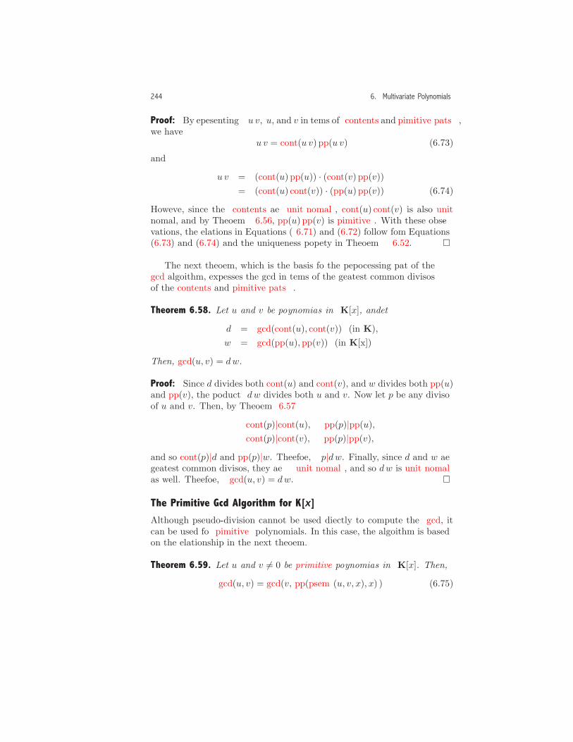
244 6. Multivariate Polynomials
Proof: By representing u v, u, and v in terms of contents and primitive parts,we have
u v = cont(u v) pp(u v) (6.73)
and
u v = (cont(u) pp(u)) · (cont(v) pp(v))= (cont(u) cont(v)) · (pp(u) pp(v)). (6.74)
However, since the contents are unit normal, cont(u) cont(v) is also unitnormal, and by Theorem 6.56, pp(u) pp(v) is primitive. With these obser-vations, the relations in Equations (6.71) and (6.72) follow from Equations(6.73) and (6.74) and the uniqueness property in Theorem 6.52. �
The next theorem, which is the basis for the preprocessing part of thegcd algorithm, expresses the gcd in terms of the greatest common divisorsof the contents and primitive parts.
Theorem 6.58. Let u and v be polynomials in K[x], and let
d = gcd(cont(u), cont(v)) (in K),w = gcd(pp(u), pp(v)) (in K[x]).
Then, gcd(u, v) = dw.
Proof: Since d divides both cont(u) and cont(v), and w divides both pp(u)and pp(v), the product dw divides both u and v. Now let p be any divisorof u and v. Then, by Theorem 6.57
cont(p)|cont(u), pp(p)|pp(u),cont(p)|cont(v), pp(p)|pp(v),
and so cont(p)|d and pp(p)|w. Therefore, p|dw. Finally, since d and w aregreatest common divisors, they are unit normal, and so dw is unit normalas well. Therefore, gcd(u, v) = dw. �
The Primitive Gcd Algorithm for K[x]Although pseudo-division cannot be used directly to compute the gcd, itcan be used for primitive polynomials. In this case, the algorithm is basedon the relationship in the next theorem.
Theorem 6.59. Let u and v �= 0 be primitive polynomials in K[x]. Then,
gcd(u, v) = gcd(v, pp(psrem(u, v, x), x) ). (6.75)

6.3. Greatest Common Divisors 245
Proof: Let r = psrem(u, v, x). To prove the theorem, we show that the twopairs of polynomials u, v and v, pp(r, x) have the same common divisors.
Let p be a polynomial that divides u and v. Observe that p is primitivebecause it divides a primitive polynomial (Exercise 8). In addition, since
lc(v, x)δ u = psquot(u, v, x) v + r, (6.76)
p|r, and there is a polynomial s such that r = p s. By Theorem 6.57,
pp(r, x) = pp(p s, x) = pp(p, x) pp(s, x) = p · pp(s, x),
and so p|pp(r, x).Next, let’s suppose that p divides v and pp(r, x) where, by Exercise 8,
p is primitive. Therefore, by Equation (6.76), p|lc(v, x)δ u, and there is apolynomial s such that
lc(v, x)δ u = s p
= cont(s, x) pp(s, x) cont(p, x) pp(p, x)= cont(s, x) pp(s, x) p
where, by Theorem 6.56, the product pp(s, x) p is primitive. Since u isprimitive and since cont(s, x) is unit normal, Theorem 6.52 implies
c lc(v, x)δ = cont(s, x)
where c is the unique unit inK so that c lc(v, x)δ is unit normal. Therefore,
u = pp(u) = c pp(s, x) p,
and p|u.This analysis shows that the polynomials u and v and the polynomials
v and pp(r, x) have the same common divisors, and therefore gcd(u, v) =gcd(v, pp(r, x)). �
The next example shows that the pp operator in Equation (6.75) is re-quired since the pseudo-division of a primitive polynomial u by a primitivepolynomial v may give a pseudo-remainder that is not primitive.
Example 6.60. The polynomials
u = x2 + x+ (y + 1), v = x2y2 + x
are primitive in Z[x, y] with main variable x. Then,

246 6. Multivariate Polynomials
psrem(u, v, x) = (y2 − 1)x+ y2 (y + 1)
which is not primitive. �
We describe now a gcd algorithm for polynomials that is based on The-orems 6.58 and 6.59. Let u and v be two non-zero polynomials in K[x].First, compute
d = gcd(cont(u, x), cont(v, x)). (6.77)
This step, which constitutes the preprocessing step of the algorithm, usesa gcd algorithm in the coefficient domain K to compute the contents andthe gcd in Equation (6.77). Next, when v �= 0, consider the remaindersequence:
R−1 = pp(u),R0 = pp(v),R1 = pp(psrem(R−1, R0, x)),
... (6.78)Ri = pp(psrem(Ri−2, Ri−1, x)),
...
This sequence is called the primitive remainder sequence because each ofthe remainders is primitive. Since pseudo-division satisfies the Euclideanproperty, there is some remainder in this sequence which is zero. LetRρ = 0 be the first such remainder. By Theorem 6.59,
gcd(pp(u), pp(v)) = gcd(R−1, R0)= gcd(R0, R1)... (6.79)= gcd(Rρ−1, Rρ) = gcd(Rρ−1, 0)= Rρ−1
where Rρ−1 is the non-normalized form of the gcd. Therefore, by Theorem6.58 and Equation (6.77),
gcd(u, v) = c · d · Rρ−1
where the unit c in K transforms the gcd to unit normal form.This discussion is summarized in the following theorem.

6.3. Greatest Common Divisors 247
Theorem 6.61. Let u and v be polynomials in K[x] at least one of which isnon-zero, and let
d = gcd(cont(u, x), cont(v, x)). (6.80)
Then,gcd(u, v) = c · d ·Rρ−1 (6.81)
where c is the unique unit so that transforms the gcd to unit normal form.
Proof: Although the theorem was derived assuming v �= 0, it is true whenu �= 0 and v = 0 as well. In this case, ρ = 0 and
Rρ−1 = pp(u), d = cont(u).
Therefore,
gcd(u, 0) = c · d · Rρ−1 = c · cont(u) pp(u) = c u
where c transforms u to unit normal form. �
The algorithm based on Equations (6.78), (6.79), (6.80), and (6.81)is called the primitive gcd algorithm because the remainders in Equa-tion (6.78) are primitive.
Example 6.62. Let
u = −yx2 + y3, v = yx2 + 2y2x+ y3
be polynomials in Z[x, y] with main variable x. Then,
cont(u, x) = y, cont(v, x) = y,
d = gcd(cont(u, x), cont(v, x)) = y,
R−1 = pp(u, x) = −x2 + y2,
R0 = pp(v, x) = x2 + 2yx+ y2,
and
R1 = pp(psrem(R−1, R0, x), x)= pp(2 y2 + 2 y x, x)= y + x,
R2 = pp(psrem(R0, R1, x), x)= pp(0, x)= 0.

248 6. Multivariate Polynomials
At this point, the process terminates, and using Equation (6.81),
gcd(u, v) = dR1 = y x+ y2. �
The Mv poly gcd and Mv poly gcd rec Procedures. Procedures that obtainthe gcd in the multivariate polynomial domain K[x1, . . . , xp] when K iseither Z or Q are given in Figures 6.6 and 6.7. The input polynomialsare multivariate polynomials (in expanded form) in the symbols in the listL where the first symbol in L is the main variable. The main procedureMv poly gcd handles some simple cases in lines 1–4, and, at line 6, calls onthe recursive procedure Mv poly gcd rec which performs the calculations.The Normalize operator in lines 2, 4, and 6, which transforms the gcd tounit normal form, is described in Exercise 12. Since the unit normal formdepends on the base coefficient domain, the domain variable K is includedin the parameter list for Normalize.
The procedure Mv poly gcd rec, which returns the greatest commondivisor in non-normalized form, is highly recursive because the contentcomputations in lines 7, 8, and 17 and the gcd computation in line 9 in-volve recursive calls on the procedure. (The Polynomial content operatoris described in Exercise 7.)
Procedure Mv poly gcd(u, v, L,K);Input
u, v : multivariate polynomials with variables in L and coefficientsin Z or Q;
L : list of symbols;K : the symbol Z or Q;
Outputgcd(u, v);
Begin1 if u = 0 then2 Return(Normalize(v, L,K))3 elseif v = 0 then4 Return(Normalize(u,L,K))5 else6 Return(Normalize(Mv poly gcd rec(u, v, L,K), L, K))
End
Figure 6.6. The main MPL procedure that obtains the gcd of two multivari-ate polynomials with coefficients in Z or Q. (Implementation: Maple (txt),Mathematica (txt), MuPAD (txt).)

6.3. Greatest Common Divisors 249
Procedure Mv poly gcd rec(u, v, L,K);Input
u, v : non-zero multivariate polynomials with variables in L andcoefficients in Z or Q;
L : a list of symbols;K : the symbol Z or Q;
Outputgcd(u, v) (not normalized);
Local Variablesx,R, cont u, cont v , d, pp u, pp v , r, pp r, cont r ;
Begin1 if L = [ ] then2 if K = Z then Return(Integer gcd(u, v))3 elseif K = Q then Return(1)4 else5 x := First(L);6 R := Rest(L);7 cont u := Polynomial content(u, x,R,K);8 cont v := Polynomial content(v, x,R,K);9 d := Mv poly gcd rec(cont u, cont v , R,K);10 pp u := Rec quotient(u, cont u, L,K);11 pp v := Rec quotient(u, cont v , L,K);12 while pp v �= 0 do13 r := Pseudo remainder(pp u, pp v , x);14 if r = 0 then15 pp r := 016 else17 cont r := Polynomial content(r, x,R,K);18 pp r := Rec quotient(u, cont r , L,K);19 pp u := pp v ;20 pp v := pp r ;21 Return(Algebraic expand(d ∗ pp u))
End
Figure 6.7. The MPL procedure that obtains a (non-normalized) gcd of twomultivariate polynomials with coefficients in Z or Q. (Implementation: Maple(txt), Mathematica (txt), MuPAD (txt).)
Lines 1–3 provide a termination condition for the recursion. When theinput list L is empty, the input expressions are in the base coefficient domain.When this domain is Z, we return the gcd of the two integers (line 2), andwhen the domain is Q, we simply return the integer 1 (line 3).

250 6. Multivariate Polynomials
In lines 5–9, we obtain the expression d in Equation (6.80), and, inlines 10–11, we obtain the primitive parts of the input polynomials. Inlines 12–20, we form the polynomial remainder sequence (6.78), and, inline 21, we obtain the gcd in non-normalized form using Equation (6.81).(The constant c that obtains the normalized form is obtained in Normalizeat line 6 of Mv poly gcd .)
Appraisal of the Algorithm
In Example 4.26 on page 130 we showed that the gcd algorithm in Q[x]exhibits a phenomenon called coefficient explosion where succeeding poly-nomials in the remainder sequence have coefficients that require more andmore digits. The next example shows that this problem can be even morepronounced for multivariate polynomials.
Example 6.63. Consider the polynomials
u = x3y2 + 6 x4y + 9 x5 + 4 x2y2 + 24 x3y + 36 x4 + 5 xy2 + 30 yx2
+45 x3 + 2 y2 + 12 y x+ 18 x2,
v = x5y2 + 8 x4y + 16 x3 + 12 x4y2 + 96 x3y + 192 x2 + 45 x3y2
+360 yx2 + 720 x+ 50 x2y2 + 400 y x+ 800
as polynomials in Z[x, y] with x the main variable. Observe that
deg(u, x) = 5, deg(u, y) = 2, deg(v, x) = 5, deg(v, y) = 2,
and the maximum number of digits in the integer coefficients in u and vis 3.
By collecting coefficients in powers of x, we obtain
u = 9 x5 + (6 y + 36)x4 +(y2 + 24 y + 45
)x3 +
(4 y2 + 30 y + 18
)x2
+(5 y2 + 12 y
)x+ 2 y2,
v = y2 x5 +(8 y + 12 y2
)x4 +
(96 y + 16 + 45 y2
)x3
+(192 + 50 y2 + 360 y
)x2 + (720 + 400 y)x+ 800.
In this form, we see that
cont(u, x) = 1, cont(v, x) = 1,
and so,d = gcd(cont(u, x), cont(v, x)) = 1.

6.3. Greatest Common Divisors 251
Therefore, R−1 = u and R0 = v, and at the first iteration, we have (incollected form)
r = psrem(R−1, R0, x)=
(−72 y− 72 y2 + 6 y3)x4
+(y4 − 360 y2 − 144− 864 y + 24 y3
)x3
+(4 y4 − 3240 y− 1728 + 30 y3 − 432 y2
)x2
+(5 y4 − 6480− 3600 y+ 12 y3
)x
+2 y4 − 7200.
Although pseudo-division has decreased the degree in the main variable xby 1, it has increased the degree in y to 4 and increased the size of theinteger coefficients. Because of this, the content computation at line 17 ofMv poly gcd rec involves coefficient explosion of up to 7 digits. Since thecontent of this polynomial is 1, we have R1 = r.
At the next iteration, we obtain
r = psrem(R0, R1, x)=
(− 6048 y6 + y10 + 672 y8 − 2448 y7 + 20736 y2
− 48 y9 + 82944 y3 + 221184 y4 + 29376 y5)x3
+(4 y10 + 57024 y5 − 89856 y6 + 2040 y8 + 4464 y7
+995328 y3 + 248832 y2 − 192 y9 + 1254528 y4)x2
+(− 144288 y6 + 1848 y8 + 5 y10 − 176256 y5
+1710720 y4− 240 y9 + 19296 y7 + 3732480 y3
+933120 y2)x
+1036800 y2− 345600 y5 + 22464 y6 + 172800 y4
+912 y8 − 96 y9 + 2 y10 + 1152 y7 + 4147200 y3.
Again, pseudo-division has decreased the degree in x by 1, but has increasedthe degree in y to 10, and has increased the size of the integer coefficients.At this step, the content computation at line 17 involves coefficients withup to 41 digits. Since the content of this polynomial is y2, we have
R2 = Rec quotient(r, y2, [x, y]).
The iteration continues until R5 = 0. The coefficient and degree explo-sion for the remaining iterations is summarized in Figure 6.8. Observe that,at iterations 3 and 4, the remainder r involves more coefficient explosionand degree explosion in y (columns 2 and 4). In addition, the degree of

252 6. Multivariate Polynomials
i Max. Digits deg(r, x) deg(r, y) deg(cont(r), y) Max. Digitsr in computation
(line 13) (line 13) (line 13) (line 17) of cont r(line 17)
1 4 4 4 0 7
2 7 3 10 2 41
3 14 2 18 10 44
4 17 1 24 24 17
5 1 −∞ −∞ −∞ 1
Figure 6.8. The degree and coefficient explosion in the procedure Mv poly gcd recfor the polynomials in Example 6.63.
the content increases (column 5), and the most significant coefficient ex-plosion occurs during the content computation (column 6). Although, atthe fourth iteration deg(r, y) = 24, all of this involves content, and oncethis content is removed, the algorithm obtains
gcd(u, v) = x+ 2. �
The Subresultant gcd Algorithm in K[x]There are two competing actions at work in the gcd algorithm that affectthe coefficient and degree explosion. First, the content computation anddivision at lines 17–18 of Mv poly gcd rec tend to reduce the size of theremainders. On the other hand, the content computation for these remain-ders involves significant coefficient explosion and degree explosion in theauxiliary variables.
We describe now another approach that avoids the content computationof the pseudo-remainders but still tends to reduce the size of the remain-ders. The algorithm is known as the subresultant gcd algorithm because itsmathematical justification is based on a mathematical concept with thisname. Since the mathematics behind this algorithm is quite involved, weonly describe the algorithm and refer the reader to the references cited atthe end of the chapter for the mathematical details.
Let u and v be in K[x]. As before, we first compute
d = gcd(cont(u, x), cont(v, x)), (6.82)
and, for this algorithm, compute
g = gcd(lc(u, x), lc(v, x)) (6.83)
where the gcd and content computations are done in K. For v �= 0 anddeg(u, x) ≥ deg(v, x), this approach replaces the sequence in Equation (6.78)
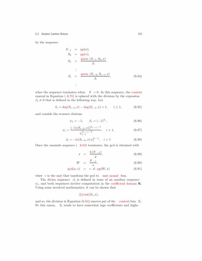
6.3. Greatest Common Divisors 253
by the sequence
S−1 = pp(u),S0 = pp(v),
S1 =psrem(S−1, S0, x)
β1,
...
Si =psrem(Si−2, Si−1, x)
βi, (6.84)
...
where the sequence terminates when Sρ = 0. In this sequence, the contentremoval in Equation (6.78) is replaced with the division by the expressionβi �= 0 that is defined in the following way. Let
δi = deg(Si−2, x)− deg(Si−1, x) + 1, i ≥ 1, (6.85)
and consider the recurrence relations
ψ1 = −1, β1 = (−1)δ1 , (6.86)
ψi =(−lc(Si−2, x))δ(i−1)−1
ψδ(i−1)−2
i−1
, i > 1, (6.87)
βi = −lc(Si−2, x)ψδi−1i , i > 1. (6.88)
Once the remainder sequence (6.84) terminates, the gcd is obtained with
s =lc(Sρ−1)
g, (6.89)
W =Sρ−1
s, (6.90)
gcd(u, v) = c · d · pp(W,x) (6.91)
where c is the unit that transforms the gcd to unit normal form.The divisor sequence βi is defined in terms of an auxiliary sequence
ψi, and both sequences involve computation in the coefficient domain K.Using some involved mathematics, it can be shown that
βi|cont(Si, x),and so, the division in Equation (6.84) removes part of the content from Si.For this reason, Si tends to have somewhat larger coefficients and higher

254 6. Multivariate Polynomials
degree in the auxiliary variables than Ri. On the other hand, βi does notinvolve a gcd computation which significantly reduces the coefficient anddegree explosion in K. These points are illustrated in Example 6.64 below.
Finally, this approach requires that deg(u, x) ≥ deg(v, x), and whenthis is not so, it is necessary to interchange u and v.
The Sub resultant gcd rec Procedure. In Figures 6.9 and 6.10, we give aprocedure that uses this algorithm to obtain a gcd in the multivariatepolynomial domain K[x1, . . . , xp] when K is either Z or Q. The procedure,which is similar to the procedure for Mv poly gcd rec in Figure 6.7, returnsthe gcd in non-normalized form. The normalized form is obtained using theprocedure Mv poly gcd (Figure 6.6) with Mv poly gcd rec at line 6 replacedby Sub resultant gcd rec.
In lines 6–11, we select U and V so that deg(U, x) ≥ deg(V, x). Inlines 13–15 we obtain d in Equation (6.82) using the Polynomial content sroperator described in Exercise 7 and a recursive call on the procedure. Theremainder sequence is initialized in lines 16–17, and g in Equation (6.83) isobtained in line 18. In lines 19–38, we obtain the remainder sequence (6.84)where βi and ψi are obtained in lines 23–32. Finally, a non-normalized formof the gcd is obtained in lines 39–43 using Equations (6.89), (6.90), and(6.91). (The constant c that obtains the normalized form is obtained inNormalize at line 6 of Mv poly gcd .)
Example 6.64. Consider the gcd calculation for the polynomials in Ex-ample 6.63. In Figure 6.11 we summarize the degree and coefficient explo-sion obtained by Sub resultant gcd rec in the pseudo-remainder calculation(line 21) and β calculation (lines 26 and 32).
Comparing these results with those in Figure 6.8, we see, for this pro-cedure, the remainder r involves coefficient explosion (column 2) of up to24 digits and degree explosion (column 4) up to degree 32. This is some-what larger than for r in Mv poly gcd rec which involves up to 17 digitsand degree 24.
On the other hand, β involves coefficient explosion (column 6) of upto 11 digits and degree explosion (column 5) up to degree 16, which is sig-nificantly smaller than the computation of cont r in Mv poly gcd rec, whichinvolves up to 44 digits and degree 24. Because of this, the computationtime for this example for Sub resultant gcd rec is about one third the timefor Mv poly gcd rec. �
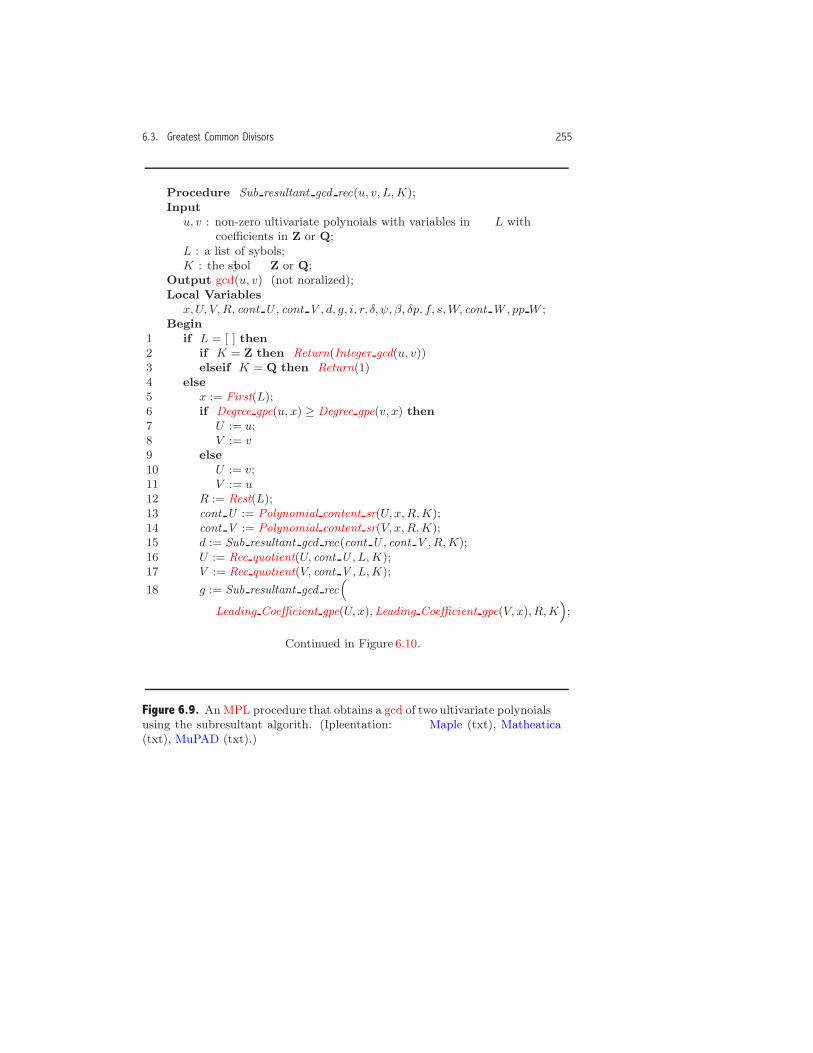
6.3. Greatest Common Divisors 255
Procedure Sub resultant gcd rec(u, v, L,K);Input
u, v : non-zero multivariate polynomials with variables in L withcoefficients in Z or Q;
L : a list of symbols;K : the symbol Z or Q;
Output gcd(u, v) (not normalized);Local Variables
x,U, V,R, cont U , cont V , d, g, i, r, δ, ψ, β, δp, f, s,W, cont W , pp W ;Begin
1 if L = [ ] then2 if K = Z then Return(Integer gcd(u, v))3 elseif K = Q then Return(1)4 else5 x := First(L);6 if Degree gpe(u, x) ≥ Degree gpe(v, x) then7 U := u;8 V := v9 else10 U := v;11 V := u12 R := Rest(L);13 cont U := Polynomial content sr(U, x,R,K);14 cont V := Polynomial content sr(V, x,R,K);15 d := Sub resultant gcd rec(cont U , cont V , R,K);16 U := Rec quotient(U, cont U , L,K);17 V := Rec quotient(V, cont V , L,K);
18 g := Sub resultant gcd rec
Leading Coefficient gpe(U, x),Leading Coefficient gpe(V, x),R,K ;
Continued in Figure 6.10.
Figure 6.9. An MPL procedure that obtains a gcd of two multivariate polynomialsusing the subresultant algorithm. (Implementation: Maple (txt), Mathematica(txt), MuPAD (txt).)
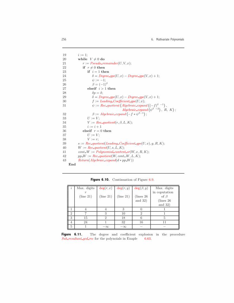
256 6. Multivariate Polynomials
19 i := 1;20 while V �= 0 do21 r := Pseudo remainder(U, V, x);22 if r �= 0 then23 if i = 1 then24 δ = Degree gpe(U, x) −Degree gpe(V, x) + 1;25 ψ := −1;26 β = (−1)δ
27 elseif i > 1 then28 δp = δ;29 δ = Degree gpe(U, x) −Degree gpe(V, x) + 1;30 f := Leading Coefficient gpe(U,x);31 ψ := Rec quotient Algebraic expand (−f)δp−1 ,
Algebraic expand ψδp−2 , R, K ;
32 β := Algebraic expand −f ∗ ψδ−1 ;33 U := V ;34 V := Rec quotient(r, β, L,K);35 i := i + 136 elseif r = 0 then37 U := V ;38 V := r;39 s := Rec quotient(Leading Coefficient gpe(U, x), g, R,K);40 W := Rec quotient(U, s, L,K);41 cont W := Polynomial content sr(W,x,R,K);42 pp W := Rec quotient(W, cont W , L,K);43 Return(Algebraic expand(d ∗ pp W ))
End
Figure 6.10. Continuation of Figure 6.9.
i Max. digits deg(r, x) deg(r, y) deg(β, y) Max. digitsr in computation
(line 21) (line 21) (line 21) (lines 26 of βand 32) (lines 26
and 32)
1 4 4 3 0 1
2 7 3 10 2 1
3 15 2 18 6 5
4 24 1 32 16 11
5 1 −∞ −∞ − −
Figure 6.11. The degree and coefficient explosion in the procedureSub resultant gcd rec for the polynomials in Example 6.63.

6.3. Greatest Common Divisors 257
Because of coefficient and degree explosion, gcd computation for polyno-mials with large coefficients and many variables of high degree is a difficultproblem. There are, however, more sophisticated algorithms that obtainthe gcd more efficiently than those given here. The references cited at theend of the chapter survey some of the recent developments for this problem.
Rational Simplification
One application of multivariate polynomial gcd computation is to obtainthe rationally simplified form of an algebraic expression. Consider the classof expressions RS-IN defined by the following rules.
RS-IN-1. u is an integer.
RS-IN-2. u is a fraction.
RS-IN-3. u is a symbol.
RS-IN-4. u is sum with operands that are in RS-IN.
RS-IN-5. u is a product with operands that are in RS-IN.
RS-IN-6. u is a power with a base that is in RS-IN and exponent that isan integer.
In the next definition we describe a standard form for expressions inRS-IN.
Definition 6.65. Let u be an expression in RS-IN. The expression u is inrationally simplified form if it satisfies one of the following rules.
RS-1. u is a multivariate polynomial with integer coefficients.
RS-2. Letn = Numerator(u), d = Denominator(u).
Then, n and d satisfy the following:
1. n and d are multivariate polynomials in a list of symbols L withinteger coefficients.
2. d �= 0 and d �= 1.
3. n and d are relatively prime.
4. n and d are in unit normal form.
RS-3. u = (−1) v where v satisfies RS-2.

258 6. Multivariate Polynomials
The process of transforming an expression in the class RS-IN to a ra-tionally simplified form in the class RS is called rational simplification.
Example 6.66. The following transformations illustrate the rational sim-plification process:
−4 a2 + 4 b2
8 a2 − 16 a b+ 8 b2→ − a+ b
2 a− 2 b, L = [a, b], (6.92)
→ a+ b
2 b− 2 a, L = [b, a], (6.93)
1(1a+
c
a b
) +a b c+ ac2
(b+ c)2→ a, L = [a, b, c],
2 a3 + 22 a b+ 6 a2 + 7 a+ 6 a2b+ 12 b2 + 21 b7 a2 − 2 a2b− 5 a− 5 a b2 + 21 a b− 15 b+ 3 b3
(6.94)
→ 2 a2 + 4 b+ 6 a+ 77 a− 2 a b+ b2 − 5
, L = [b, a].
The expression to the right of the arrow is in rationally simplified form. Ineach case the variable order is indicated by a list L where the main variableis the first symbol in L. Observe that in Equations (6.92) and (6.93), therational simplified form depends on the variable order. In Equation (6.94),there is a common factor of a+3 b in the numerator and denominator. �
In Exercise 13 we describe a procedure that obtains the rationally sim-plified form of an expression.
The Extended Euclidean Algorithm in K[x]When the coefficient domain is a field, using the extended Euclidean algo-rithm, we obtain polynomials A and B such that Au + B v = gcd(u, v).When the coefficient domain is not a field, this relationship takes the fol-lowing form.
Theorem 6.67. Let u and v be polynomials in K[x]. Then, there arepolynomials A and B in K[x] and a unit normal expression s in K suchthat
Au+B v = s gcd(u, v). (6.95)

6.3. Greatest Common Divisors 259
Proof: A constructive proof of the theorem is similar to the proofs forTheorem 2.12 (page 24) and Theorem 4.27 (page 132) with modificationsto accommodate the properties of the coefficient domain K. The details ofthe proof are left to the reader (Exercise 14). �
Example 6.68. Consider the polynomials
u = −4 x3y + 4 xy3 + 4 xy, v = 6 x4y + 12 x3y2 + 6 y3x2
in Z[x, y] with main variable x. Then,
s = 24 y4 + 24 y2, gcd(u, v) = 2 xy,
A = 12 y2+24 y4x2+24 y5x+12 y2x2, B = 16 y4x+8 xy2−16 y5−16 y3.
�
The next theorem extends the divisor properties described in Theorem6.10 (page 205) from the coefficient domain K to K[x].
Theorem 6.69. Suppose that u, v, and w are in K[x] with w|u v.1. If w and u are relatively prime, then w|v.2. If w is irrreducible, then w|u or w|v.
Proof: To show (1), by Theorem 6.67, there are polynomials A and B inK[x] and an s in K such that
Aw +B u = s gcd(w, u)
where, since w and u are relatively prime, s gcd(w, u) is in K. Therefore,
Aw v + B u v = s gcd(w, u) v,
and, since w divides each term in the sum, w|s gcd(w, u) v. Furthermore,Theorem 6.57 implies that
pp(w, x)|pp(s gcd(w, u), x) pp(v, x),and, since pp(s gcd(w, u), x) = 1,
pp(w, x)|pp(v, x). (6.96)
In addition, since w|u v, Theorem 6.57 implies
cont(w, x)|cont(u, x) cont(v, x).
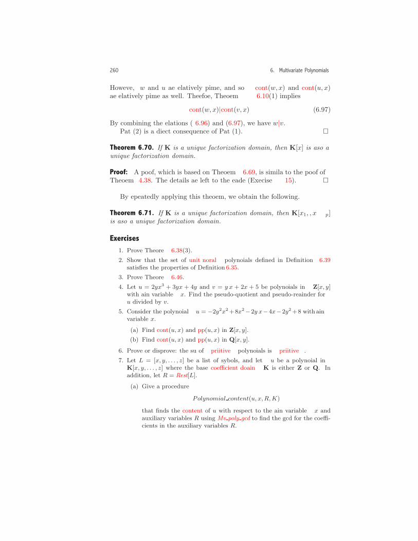
260 6. Multivariate Polynomials
However, w and u are relatively prime, and so cont(w, x) and cont(u, x)are relatively prime as well. Therefore, Theorem 6.10(1) implies
cont(w, x)|cont(v, x). (6.97)
By combining the relations (6.96) and (6.97), we have w|v.Part (2) is a direct consequence of Part (1). �
Theorem 6.70. If K is a unique factorization domain, then K[x] is also aunique factorization domain.
Proof: A proof, which is based on Theorem 6.69, is similar to the proof ofTheorem 4.38. The details are left to the reader (Exercise 15). �
By repeatedly applying this theorem, we obtain the following.
Theorem 6.71. If K is a unique factorization domain, then K[x1, . . . , xp]is also a unique factorization domain.
Exercises1. Prove Theorem 6.38(3).
2. Show that the set of unit normal polynomials defined in Definition 6.39satisfies the properties of Definition 6.35.
3. Prove Theorem 6.46.
4. Let u = 2yx3 + 3yx + 4y and v = y x + 2x + 5 be polynomials in Z[x, y]with main variable x. Find the pseudo-quotient and pseudo-remainder foru divided by v.
5. Consider the polynomial u = −2y2x2 +8x2−2y x−4x−2y2 +8 with mainvariable x.
(a) Find cont(u, x) and pp(u, x) in Z[x, y].
(b) Find cont(u, x) and pp(u, x) in Q[x, y].
6. Prove or disprove: the sum of primitive polynomials is primitive.
7. Let L = [x, y, . . . , z] be a list of symbols, and let u be a polynomial inK[x, y, . . . , z] where the base coefficient domain K is either Z or Q. Inaddition, let R = Rest[L].
(a) Give a procedure
Polynomial content(u, x,R,K)
that finds the content of u with respect to the main variable x andauxiliary variables R using Mv poly gcd to find the gcd for the coeffi-cients in the auxiliary variables R.

6.3. Greatest Common Divisors 261
(b) Give a procedure
Polynomial content sr(u, x,R,K)
that finds the content that uses the subresultant algorithm to findthe gcd for the coefficients in the auxiliary variables R.
8. Let p, u, and v be in K[x].
(a) Suppose that u is primitive and v|u. Show that v is also primitive.
(b) For p a primitive polynomial and p|gcd(u, v, x), show that
p|gcd(pp(u, x),pp(v, x), x).
9. Suppose that u and v are polynomials in K[x], and suppose that
deg(gcd(u, v), x) = 0.
Show that pp(u, x) and pp(v, x) are relatively prime.
10. Suppose that u and v are polynomials in K[x] with positive degree, andsuppose that psrem(u, v, x) = 0. Show that u and v have a common factorwith positive degree.
11. Let u and v be polynomials in K[x]. Show that
(a) gcd(cont(u, x), cont(v, x), x) = cont(gcd(u, v, x), x).
(b) gcd(pp(u, x),pp(v, x), x) = pp(gcd(u, v, x), x).
12. Let u be a polynomial in K[x, y, . . . , z] with x the main variable where thecoefficient domain K is either Z or Q, and let L = [x, y, . . . , z]. Give aprocedure
Normalize(u,L,K)
that finds the unit normal form of u. If u = 0, return 0. Note: Thenormalized form depends on the base coefficient domain.
13. Let u be an expression that satisfies the RS-IN rules on page 257, and letL be the list of the symbols in u. Give a procedure Rational simplify(u,L)that transforms u to rationally simplified form. If a division by zero isencountered, return the global symbol Undefined.
14. Prove Theorem 6.67 using the following approach. Assume that
deg(u, x) ≥ deg(v, x),
and consider the remainder sequence
T−1 = u,
T0 = v,
T1 = psrem(pp(T−1, x),pp(T0, x), x),
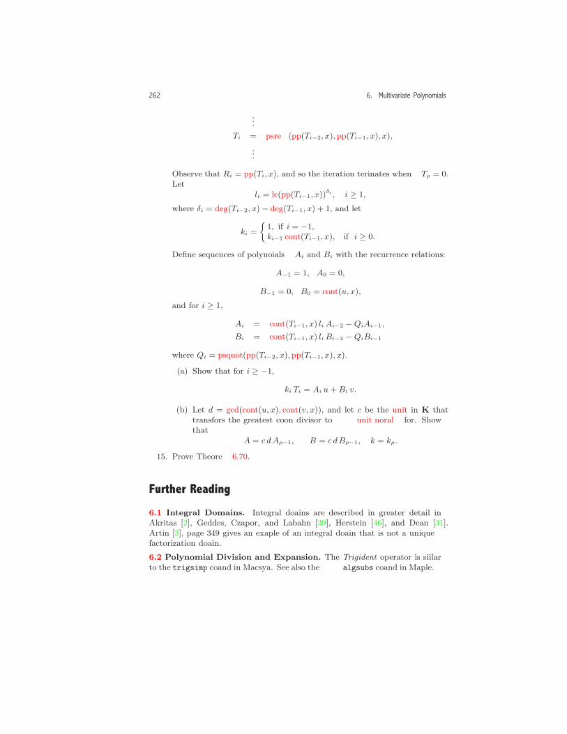
262 6. Multivariate Polynomials
...
Ti = psrem(pp(Ti−2, x),pp(Ti−1, x), x),
...
Observe that Ri = pp(Ti, x), and so the iteration terminates when Tρ = 0.Let
li = lc(pp(Ti−1, x))δi , i ≥ 1,
where δi = deg(Ti−2, x) − deg(Ti−1, x) + 1, and let
ki =1, if i = −1,ki−1 cont(Ti−1, x), if i ≥ 0.
Define sequences of polynomials Ai and Bi with the recurrence relations:
A−1 = 1, A0 = 0,
B−1 = 0, B0 = cont(u, x),
and for i ≥ 1,
Ai = cont(Ti−1, x) li Ai−2 −QiAi−1,
Bi = cont(Ti−1, x) li Bi−2 −QiBi−1
where Qi = psquot(pp(Ti−2, x),pp(Ti−1, x), x).
(a) Show that for i ≥ −1,
ki Ti = Ai u + Bi v.
(b) Let d = gcd(cont(u, x), cont(v, x)), and let c be the unit in K thattransforms the greatest common divisor to unit normal form. Showthat
A = c dAρ−1, B = c dBρ−1, k = kρ.
15. Prove Theorem 6.70.
Further Reading
6.1 Integral Domains. Integral domains are described in greater detail inAkritas [2], Geddes, Czapor, and Labahn [39], Herstein [46], and Dean [31].Artin [3], page 349 gives an example of an integral domain that is not a uniquefactorization domain.
6.2 Polynomial Division and Expansion. The Trigident operator is similarto the trigsimp command in Macsyma. See also the algsubs command in Maple.

6.3. Greatest Common Divisors 263
6.3 Greatest Common Divisors. The approach here is similar to the approach
in Knuth [55]. The subresultant algorithm presented here is given in Brown [14],
[15], Brown and Traub [16], and Collins [25], [27]. For modern developments
in gcd calculations, see Akritas [2], Geddes, Czapor, and Labahn [39], von zur
Gathen and Gerhard [96], Winkler [101], Yap [105], and Zippel [108].


7
The Resultant
In this chapter we introduce the concept of the resultant of two polynomials.The resultant has applications in calculations with algebraic numbers, thefactorization of polynomials with coefficients in algebraic number fields, thesolution of systems of polynomial equations, and the integration of rationalfunctions.
The resultant of polynomials u and v is formally defined in Section 7.1as the determinant of a matrix whose entries depend on the coefficients ofthe polynomials. In addition, we describe a Euclidean type algorithm thatobtains the resultant without a determinant calculation. In Section 7.2, weuse resultants to find polynomial relations for explicit algebraic numbers.
7.1 The Resultant Concept
Suppose that we are given two polynomials
u = x2 + t x+ 2, v = x2 + 5 x+ 6,
and want to know for which values of t the polynomials have a commonfactor with positive degree. Since the polynomials do not have a commonfactor for all values of t, a greatest common divisor algorithm cannot beused for this purpose. In this section, we introduce the resultant of twopolynomials which provides a way to determine t.
Let’s generalize things a bit. Let u and v be polynomials in F[x] withdegree 2:
u = u2 x2 + u1 x+ u0, v = v2 x
2 + v1 x+ v0.
265

266 7. The Resultant
Our goal is to find a function of the coefficients of the two polynomialsthat determines if there is a common factor. Suppose, for the moment,that gcd(u, v) = 1. Then, by Theorem 4.36 on page 137, there are uniquepolynomials A(x) and B(x) with deg(A) < deg(v) and deg(B) < deg(u)such that
Au+B v = 1. (7.1)
With A = a1 x+ a0 and B = b1 x+ b0, Equation (7.1) becomes
(a1 x+ a0) (u2 x2 + u1 x+ u0) + (b1 x+ b0) (v2 x
2 + v1 x + v0) = 1.
Expanding the left side of this equation and comparing the coefficients ofpowers of x, we obtain a system of linear equations:
u2 a1 + v2 b1 = 0, (coefficient of x3),u1 a1 + u2 a0 + v1 b1 + v2 b0 = 0, (coefficient of x2),u0 a1 + u1 a0 + v0 b1 + v1 b0 = 0, (coefficient of x1),
u0 a0 + v0 b0 = 1, (coefficient of x0).
In matrix form these equations become:
M
a1
a0
b1b0
=
0001
, (7.2)
where M is the matrix of coefficients
M =
u2 0 v2 0u1 u2 v1 v2
u0 u1 v0 v1
0 u0 0 v0
.
Since the polynomials A and B are the unique solution to Equation (7.1),the system (7.2) also has a unique solution. Therefore, when gcd(u, v) = 1,we have det(M) �= 0.
Conversely, if we assume that det(M) �= 0, then Equation (7.2) hasa solution, which implies that Equation (7.1) has a solution, and so byTheorem 4.30 on page 133, u and v are relatively prime.
The value det(M) is called the resultant of the polynomials u and v.In practice, we usually work with the transpose of the matrix M , which isobtained by interchanging the rows and columns
MT =
u2 u1 u0 00 u2 u1 u0
v2 v1 v0 00 v2 v1 v0
.

7.1. The Resultant Concept 267
Since det(MT ) = det(M), the determinant of the transpose gives an iden-tical result.
Example 7.1. Let’s return to the problem proposed at the beginning of thesection with u = x2 + t x+ 2 and v = x2 + 5 x+ 6. Since we want u and vto have a common factor, their resultant must be 0. Therefore,
det(MT ) = det
1 t 2 00 1 t 21 5 6 00 1 5 6
= 6 t2 − 40 t+ 66 = 0.
This equation has the roots t = 3, 11/3, which are the values of t for whichu and v have a common factor. For t = 3, the common factor is x+2, andfor t = 11/3, the common factor is x+ 3. �
The resultant concept is formally described in the next two definitions.
Definition 7.2. Let K be a coefficient domain,1 and let
u(x) = umxm + um−1x
m−1 + · · ·+ u0,
v(x) = vnxn + vn−1x
n−1 + · · ·+ v0
be polynomials in K[x] with m = deg(u) > 0 and n = deg(v) > 0. Definethe matrix
S(u, v, x) =
um um−1 · · · u0
um um−1 · · · u0
. . . . . .um um−1 · · · u0
vn vn−1 · · · v0
vn vn−1 · · · v0
. . . . . .vn vn−1 · · · v0
(7.3)
which has n rows of u’s coefficients and m rows of v’s coefficients. Theblank locations in the matrix contain zeroes. The matrix S(u, v, x) is calledthe Sylvester matrix2 of the two polynomials u and v.
1In this section, the coefficient domain K satisfies the properties on page 231.2The matrix is named after the mathematician James Joseph Sylvester (1814- 1897)
who first studied the matrix in relation to the elimination of variables from systems ofpolynomial equations.

268 7. The Resultant
The Sylvester matrix has n + m rows and columns and is only de-fined when u and v have positive degree. For example, if deg(u) = 2 anddeg(v) = 3,
S(u, v, x) =
u2 u1 u0 0 00 u2 u1 u0 00 0 u2 u1 u0
v3 v2 v1 v0 00 v3 v2 v1 v0
.
Definition 7.3. Let u and v be non-zero polynomials in K[x], with m =deg(u) and n = deg(v). The resultant3 of u and v is defined as
res(u, v, x) =
1, if deg(u, x) = 0, deg(v, x) = 0,un0 , if deg(u, x) = 0, deg(v, x) > 0,vm0 , if deg(u, x) > 0, deg(v, x) = 0,det(S(u, v, x)), if deg(u, x) > 0, deg(v, x) > 0.
(7.4)
The resultant is not defined when either u or v is the zero polynomial.4
When there is no chance for confusion, we omit the variable x and use thenotation res(u, v).
The most important case of the definition is when both polynomialshave positive degree, and the other cases are natural extensions of thiscase. For example, if deg(u, x) = 0 and deg(v, x) > 0, then a naturalextension of the Sylvester matrix is one with n = deg(v, x) rows of u’scoefficients and m = deg(u, x) = 0 rows of v’s coefficients. Since u = u0,this matrix has the form
S =
u0 . . . 00 u0 . . . 0
. . .0 0 . . . u0
,
where there are n rows and columns. Therefore, det(S) = un0 , and so it isreasonable for this case to define res(u, v) = un0 .
Example 7.4. Let
u = 2 x+ 3, v = 4 x2 + 5 x+ 6. (7.5)3The resultant is obtained in Maple with the resultant operator, in Mathematica
with the Resultant operator, and in MuPAD with the polylib :: resultant operator.(Implementation: Maple (mws), Mathematica (nb), MuPAD (mnb).)
4In Maple, Mathematica, and MuPAD, the resultant operator returns 0 when eitheru or v is 0.

7.1. The Resultant Concept 269
The resultant is
res(u, v) = det
2 3 0
0 2 34 5 6
= 30. (7.6)
In the definition of the Sylvester matrix, we emphasized that the leadingcoefficients of u and v cannot be 0. Indeed, if the resultant is computed witha Sylvester matrix that is too large, the value may change. For example,suppose that we redefine u in Equation (7.5) as
u = c x2 + 2 x+ 3
where c is an undefined symbol. Then,
res(u, v) = det
c 2 3 00 c 2 34 5 6 00 4 5 6
= 36 c2 − 129 c+ 120. (7.7)
To return to the situation in Equation (7.5), we let c = 0, and so res(u, v) =120 rather than the value 30 obtained in Equation (7.6). �
Properties of the Resultant
The resultant satisfies the following properties.
Theorem 7.5. Let b and c be in the coefficient domain K, and let u and vbe non-zero polynomials in K[x] with m = deg(u) and n = deg(v).
1. res(u, v) = (−1)mn res(v, u).
2. res(c u, v) = cn res(u, v).
3. res(u, c v) = cm res(u, v).
4. res(x, v) = v(0).
5. If u = b (x− c), then res(u, v) = bnv(c).
6. If the coefficients of u are linear in the symbol c, then
deg(res(u, v), c) ≤ n.
7. res((x − b)u, v) = v(b) res(u, v).

270 7. The Resultant
Proof: To prove (1), we assume first that both u and v have positivedegree and show that S(v, u, x) is obtained from S(u, v, x) by m · n rowinterchanges. Let Si be the ith row of S(u, v, x) where S1, S2, . . . Sn arethe rows with coefficients of u and Sn+1, Sn+2, . . . Sn+m are the rows withcoefficients of v. Consider the following row interchanges:
S1
S2
...Sn
Sn+1
Sn+2
...Sn+m
→
Sn+1
S1
...Sn
Sn+2
Sn+3
...Sn+m
→
Sn+1
Sn+2
S1
...Sn
Sn+3
Sn+4
...Sn+m
→ · · · →
Sn+1
Sn+2
...Sn+m
S1
S2
...Sn
.
To move each Si (n + 1 ≤ i ≤ n + m) to its new place requires n rowinterchanges, and since there arem such rows to move, the row interchangeproperty for determinants implies that res(u, v) = (−1)mnres(v, u). Ifdeg(u) = 0 or deg(v) = 0, (1) can also be easily verified from the definition.
The proofs of (2) and (3), which also follow from the properties fordeterminants, are left to the reader (Exercise 5).
To show (4), we assume first that deg(v) > 0. Then, the Sylvestermatrix is the n+ 1 by n+ 1 matrix
S(x, v, x) =
1 0 · · ·0 1 0 · · ·
...· · · 1 0
vn vn−1 · · · v0
,
and, therefore,
res(x v) = det(S(x, v, x)) = v0 = v(0).
When deg(v) = 0, the relationship follows directly from the definition ofthe resultant.
To show (5), first assume that deg(v) > 0. Then,
res(b (x− c), v) = det
b −b c 0 · · ·0 b −b c 0 · · ·
...0 · · · b −b c
vn vn−1 · · · v0
.
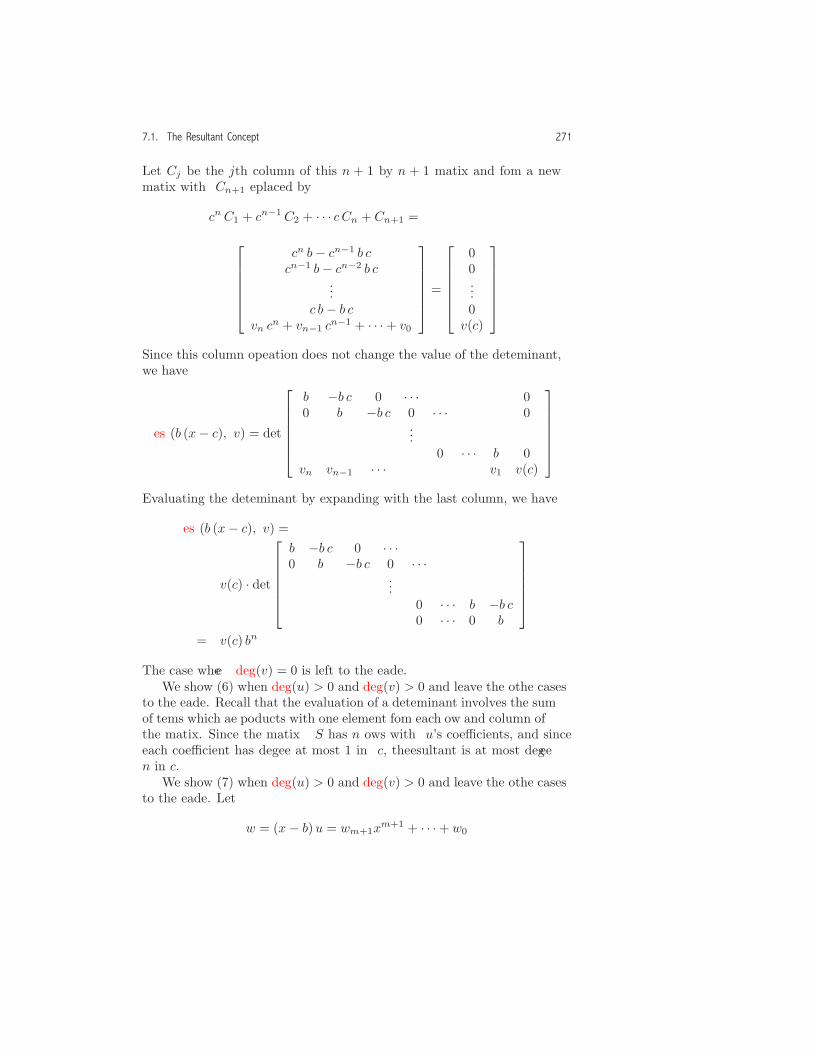
7.1. The Resultant Concept 271
Let Cj be the jth column of this n + 1 by n + 1 matrix and form a newmatrix with Cn+1 replaced by
cn C1 + cn−1 C2 + · · · cCn + Cn+1 =
cn b− cn−1 b ccn−1 b− cn−2 b c
...c b− b c
vn cn + vn−1 c
n−1 + · · ·+ v0
=
00...0
v(c)
.
Since this column operation does not change the value of the determinant,we have
res(b (x− c), v) = det
b −b c 0 · · · 00 b −b c 0 · · · 0
...0 · · · b 0
vn vn−1 · · · v1 v(c)
.
Evaluating the determinant by expanding with the last column, we have
res(b (x− c), v) =
v(c) · det
b −b c 0 · · ·0 b −b c 0 · · ·
...0 · · · b −b c0 · · · 0 b
= v(c) bn.
The case where deg(v) = 0 is left to the reader.We show (6) when deg(u) > 0 and deg(v) > 0 and leave the other cases
to the reader. Recall that the evaluation of a determinant involves the sumof terms which are products with one element from each row and column ofthe matrix. Since the matrix S has n rows with u’s coefficients, and sinceeach coefficient has degree at most 1 in c, the resultant is at most degreen in c.
We show (7) when deg(u) > 0 and deg(v) > 0 and leave the other casesto the reader. Let
w = (x − b)u = wm+1xm+1 + · · ·+ w0

272 7. The Resultant
where
wi =
{um, i = m+ 1,ui−1 − b ui, i = 1, . . . ,m,−b ui, i = 0.
(7.8)
We have res(w, v) = det(S(w, v, x)) where S(w, v, x) is the m+ 1 + n bym+ 1 + n matrix
S(w, v, x) =
wm+1 wm · · · w0
wm+1 wm · · · w0
. . . . . .wm+1 wm · · · w0
vn vn−1 · · · v0
vn vn−1 · · · v0
. . . . . .vn vn−1 · · · v0
. (7.9)
Multiplying column Ci (1 ≤ i < m+1+ n) by bm+1+n−i and adding thesecolumns to the last column, we obtain a new matrix S2 where the lastcolumn has the entries
bm+n C1 + bm+n−1 C2 + · · ·+ b Cm+n
=
bm+nwm+1 + · · ·+ bn−1 w0
...bm+1 wm+1 + · · ·+ w0
bm+n vn + · · ·+ bm v0
...bn vn + · · ·+ v0
=
bn−1w(b)...
w(b)bm v(b)
...v(b)
=
0...0
bm v(b)...
v(b)
.
We can factor v(b) out of the last column and obtain a new matrix S3
where the last column has the entries
0, . . . , 0, bm, · · · , 1,and
res(w, v) = det(S(w, v, x)) = det(S2) = v(b) · det(S3). (7.10)
Observe that det(S(w, v, x)) is a polynomial in b, and by Part (6),
deg(det(S(w, v, x)), b) ≤ n.

7.1. The Resultant Concept 273
However, since deg(v(b), b) = n, Equation (7.10) implies
deg(v(b) · det(S3), b) = deg(v(b), b) + deg(det(S3), b, )= n+ deg(det(S3), b)≤ n,
and sodeg(det(S3), b) = 0.
In other words, the symbol b is eliminated in the evaluation of det(S3).Therefore, we substitute 0 for b in S3 and obtain a new matrix S4 with them+ 1 + n entries
0, . . . , 0, 1
in the last column. From Equation (7.10), evaluating det(S4) by expandingabout the last column, we obtain
res(w, v) =
v(b) det
wm+1 wm · · · w0
wm+1 wm · · · w0
. . . . . .wm+1 wm · · · w1
vn vn−1 · · · v0
vn vn−1 · · · v0
. . . . . .vn vn−1 · · · v0
(7.11)
where the matrix has n rows of w coefficients, m rows of v coefficients, andthe last entry in row n is w1. However, when b = 0, Equation (7.8) gives
wi ={ui−1, i = 1, · · · ,m,0, i = 0,
and therefore, Equation (7.11) gives
res(w, v) = v(b) det
um um−1 · · · u0
um um−1 · · · u0
. . . . . .um um−1 · · · u1
vn vn−1 · · · v0
vn vn−1 · · · v0
. . . . . .vn vn−1 · · · v0
= v(b) res(u, v). �

274 7. The Resultant
Fundamental Theorems
The next three theorems are fundamental to the application of resultants.
Theorem 7.6. Let u and v be polynomials of positive degree in K[x]. Then,u and v have a common factor of positive degree if and only if there arenon-zero polynomials C and D in K[x] with
deg(C) < deg(v), deg(D) < deg(u) (7.12)
such thatC u+Dv = 0.
Proof: First, assume that u and v have a common factor w of positivedegree. Then, u = pw, v = q w, and so let C = −q and D = p. Therefore,C and D are non-zero and satisfy the degree conditions (7.12). In addition,
C u+Dv = −q (pw) + p (q w) = 0.
Conversely, assume that C and D exist with the properties stated inthe theorem, and suppose that u and v do not have a common factor ofpositive degree. Then, pp(u) and pp(v) are relatively prime (Exercise 9,page 261) and
pp(C) pp(u) = −pp(D) pp(v).
Using Theorem 6.69(1), we have
pp(u)|pp(D). (7.13)
But since pp(D) �= 0 and
deg(pp(D)) = deg(D) < deg(u) = deg(pp(u)),
the condition (7.13) can’t be true. Therefore, u and v have a commonfactor of positive degree. �
The next theorem is the resultant version of the relationship obtainedwith the extended Euclidean algorithm.
Theorem 7.7. Let u and v be polynomials in K[x] with deg(u) = m > 0and deg(v) = n > 0. Then, there are polynomials A and B in K[x] withdeg(A) < n and deg(B) < m such that
Au+B v = res(u, v). (7.14)
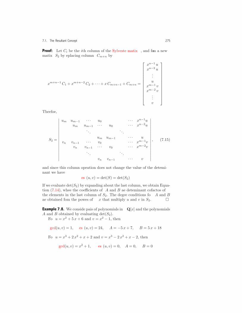
7.1. The Resultant Concept 275
Proof: Let Ci be the ith column of the Sylvester matrix, and form a newmatrix S2 by replacing column Cm+n by
xm+n−1 C1 + xm+n−2 C2 + · · ·+ xCm+n−1 + Cm+n =
xn−1 uxn−2 u
...u
xm−1 vxm−2 v
...v
.
Therefore,
S2 =
∣∣∣∣∣∣∣∣∣∣∣∣∣∣∣∣∣∣
um um−1 · · · u0 · · · xn−1uum um−1 · · · u0 · · · xn−2u
. . . . . .um um−1 · · · u
vn vn−1 · · · v0 · · · xm−1vvn vn−1 · · · v0 · · · xm−2v
. . . . . .vn vn−1 · · · v
∣∣∣∣∣∣∣∣∣∣∣∣∣∣∣∣∣∣
, (7.15)
and since this column operation does not change the value of the determi-nant we have
res(u, v) = det(S) = det(S2).
If we evaluate det(S2) by expanding about the last column, we obtain Equa-tion (7.14), where the coefficients of A and B are determinant cofactors ofthe elements in the last column of S2. The degree conditions for A and Bare obtained from the powers of x that multiply u and v in S2. �
Example 7.8. We consider pairs of polynomials inQ[x] and the polynomialsA and B obtained by evaluating det(S2).
For u = x2 + 5 x+ 6 and v = x2 − 1, then
gcd(u, v) = 1, res(u, v) = 24, A = −5 x+ 7, B = 5 x+ 18.
For u = x3 + 2 x2 + x+ 2 and v = x3 − 2 x2 + x− 2, then
gcd(u, v) = x2 + 1, res(u, v) = 0, A = 0, B = 0.

276 7. The Resultant
In this case, the polynomials A and B are not unique. Indeed
Au+B v = (−x+ 2)u+ (x + 2) v = 0. �
The next theorem describes the fundamental relationship between theresultant and the common structure (in x) of u and v.
Theorem 7.9. Let u and v be polynomials in K[x] with positive degree.Then, u and v have a common factor w with deg(w, x) > 0 if and only ifres(u, v, x) = 0.
Proof: To prove the theorem first suppose that w is a common factor of uand v with deg(w, x) > 0. Then, by Equation (7.14), w|res(u, v). However,since w has positive degree and since res(u, v) is inK, we have res(u, v) = 0.
Conversely, suppose that res(u, v) = 0. By Theorem 7.7 there are poly-nomials A and B with deg(A) < n and deg(B) < m such that
Au+B v = 0. (7.16)
Observe that if A �= 0 and B �= 0, then Theorem 7.6 implies that thereis a common factor of u and v with positive degree. Unfortunately, thepolynomials A and B obtained in Theorem 7.7 may both be zero (seeExample 7.8 above). When this occurs, we obtain a proof as follows. If
A(x) = an−1xn−1 + an−2x
n−2 + · · ·+ a0,
B(x) = bm−1xm−1 + bm−2x
m−2 + · · ·+ b0,
the matrix form of Equation (7.16) is given by
ST ·
∣∣∣∣∣∣∣∣∣∣∣∣∣∣∣∣∣∣
an−1
an−2
...a0
bm−1
bm−2
...b0
∣∣∣∣∣∣∣∣∣∣∣∣∣∣∣∣∣∣
=
00
...
00
(7.17)
where ST is the transpose of the Sylvester matrix S. Since det(ST ) =det(S) = res(u, v) = 0, the homogeneous system (7.17) has a solution withsome ai or bi not zero. This implies that there are polynomials A andB, not both zero, which satisfy Equation (7.16). In fact, Equation (7.16)

7.1. The Resultant Concept 277
implies that Au = −B v which implies that both A and B are not zero.Therefore, Theorem 7.6 implies that u and v have a common factor ofpositive degree. �
Euclidean Algorithms for Resultant Calculation
Although the resultant can be computed directly from the determinant def-inition, it can also be obtained with an algorithm similar to the Euclideanalgorithm. Since the development is simpler when the coefficient domainis a field F, we consider this case first.
Resultant Calculation in F[x]. In this case, the algorithm is based on the nexttheorem which is the resultant version of Theorem 4.22 on page 128.
Theorem 7.10. Suppose that u and v are polynomials in F[x] with posi-tive degree, where m = deg(u) and n = deg(v). Let rσ be defined by thepolynomial division
u = qσ v + rσ,
and let s = deg(rσ). Then,
res(u, v, x) ={0, if rσ = 0,(−1)mn vm−s
n res(v, rσ , x), if (rσ) �= 0. (7.18)
Proof: To verify the first case, if rσ = 0, then deg(gcd(u, v)) > 0, and byTheorem 7.9, res(u, v) = 0.
Assume next that rσ �= 0. First observe that when m < n, we haverem(u, v) = u, and the second case follows from Theorem 7.5(1).
For the remainder of the proof we assume that m ≥ n. Let’s look atthe interplay between the division process and the matrix S. Recall thatthe remainder in polynomial division is defined by the iteration scheme
ri = ri−1 − lc(ri−1)lc(v)
v xdeg(ri−1)−deg(v), r0 = u. (7.19)
Since m ≥ n, there is a least one iteration step and
r1 = u− umvn
v xm−n (7.20)
where deg(r1) ≤ m− 1. Suppose that
r1 = u(1)m−1x
m−1 + u(1)m−2x
m−2 + · · ·+ u(1)0
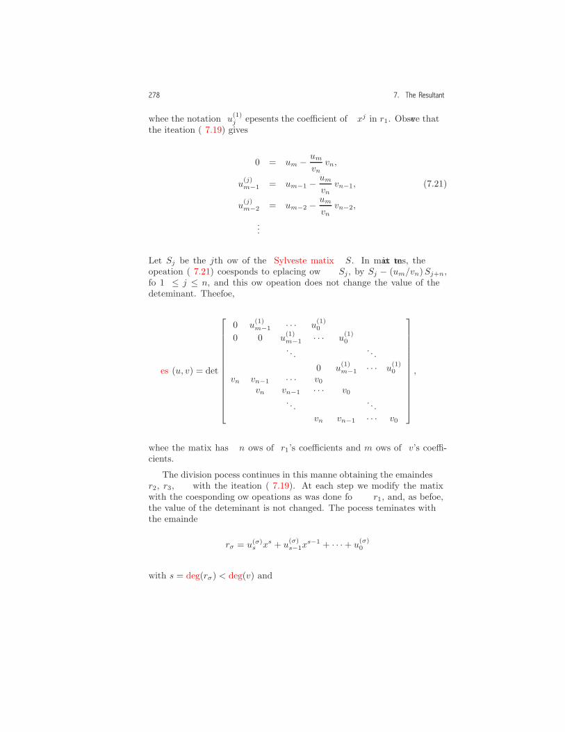
278 7. The Resultant
where the notation u(1)j represents the coefficient of xj in r1. Observe that
the iteration (7.19) gives
0 = um − umvn
vn,
u(j)m−1 = um−1 − um
vnvn−1, (7.21)
u(j)m−2 = um−2 − um
vnvn−2,
...
Let Sj be the jth row of the Sylvester matrix S. In matrix terms, theoperation (7.21) corresponds to replacing row Sj , by Sj − (um/vn)Sj+n,for 1 ≤ j ≤ n, and this row operation does not change the value of thedeterminant. Therefore,
res(u, v) = det
0 u(1)m−1 · · · u
(1)0
0 0 u(1)m−1 · · · u
(1)0
. . . . . .0 u
(1)m−1 · · · u
(1)0
vn vn−1 · · · v0
vn vn−1 · · · v0
. . . . . .vn vn−1 · · · v0
,
where the matrix has n rows of r1’s coefficients and m rows of v’s coeffi-cients.
The division process continues in this manner obtaining the remaindersr2, r3, . . . with the iteration (7.19). At each step we modify the matrixwith the corresponding row operations as was done for r1, and, as before,the value of the determinant is not changed. The process terminates withthe remainder
rσ = u(σ)s xs + u
(σ)s−1x
s−1 + · · ·+ u(σ)0
with s = deg(rσ) < deg(v) and
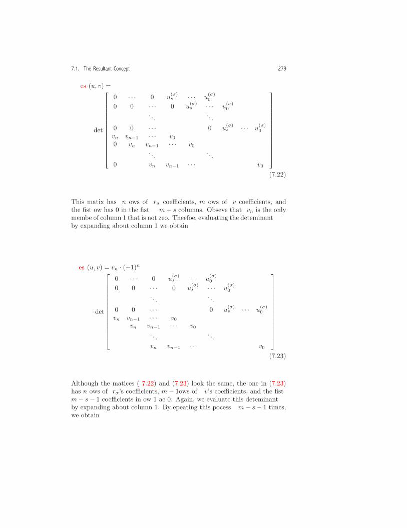
7.1. The Resultant Concept 279
res(u, v) =
det
0 · · · 0 u(σ)s · · · u
(σ)0
0 0 · · · 0 u(σ)s · · · u
(σ)0
. . . . . .0 0 · · · 0 u
(σ)s · · · u
(σ)0
vn vn−1 · · · v0
0 vn vn−1 · · · v0
. . .. . .
0 vn vn−1 · · · v0
.
(7.22)
This matrix has n rows of rσ coefficients, m rows of v coefficients, andthe first row has 0 in the first m− s columns. Observe that vn is the onlymember of column 1 that is not zero. Therefore, evaluating the determinantby expanding about column 1 we obtain
res(u, v) = vn · (−1)n
· det
0 · · · 0 u(σ)s · · · u
(σ)0
0 0 · · · 0 u(σ)s · · · u
(σ)0
. . . . . .0 0 · · · 0 u
(σ)s · · · u
(σ)0
vn vn−1 · · · v0
vn vn−1 · · · v0
. . . . . .vn vn−1 · · · v0
.
(7.23)
Although the matrices (7.22) and (7.23) look the same, the one in (7.23)has n rows of rσ ’s coefficients, m − 1 rows of v’s coefficients, and the firstm− s− 1 coefficients in row 1 are 0. Again, we evaluate this determinantby expanding about column 1. By repeating this process m− s− 1 times,we obtain

280 7. The Resultant
res(u, v) =
(vn(−1)n)m−s · det
u(σ)s · · · u
(σ)0
0 u(σ)s · · · u
(σ)0
. . . . . .· · · u
(σ)s · · · u
(σ)0
vn vn−1 · · · v0
vn vn−1 · · · v0
. . . . . .vn vn−1 · · · v0
,
(7.24)
where there are n rows of rσ’s coefficients and s = deg(rσ) rows of v’scoefficients.
Let’s assume first that deg(rσ) ≥ 1. Since the determinant in Equa-tion (7.24) is res(rσ, v), it follows from Theorem 7.5(1) that
res(u, v) = (vn(−1)n)m−s (−1)n s res(v, rσ) = (−1)nm vm−sn res(v, rσ),
which proves the second case of the theorem when deg(rσ) ≥ 1. Finally,suppose that deg(rσ) = 0. Evaluating the determinant and using Defini-tion 7.3, we obtain
res(u, v) = ((−1)nvn)m (u(σ)0 )
n= (−1)nm vmn rnσ = (−1)nmvmn res(v, rσ),
which proves the second case of the theorem. �
We can compute res(u, v) by repeatedly applying Theorem 7.10 tomembers of the polynomial remainder sequence Ri (see Equation (4.24),page 128).
Example 7.11. Let u = 2 x3−3 x+1 and v = 3 x2−4 x+3. The remaindersequence is given by
R−1 = u, R0 = v, R1 = −13/9 x− 5/3, R2 = 1962/169.
Therefore, applying Theorem 7.10, we have
res(u, v) = res(R−1, R0) = (−1)3·2 33−1 res(R0, R1)= 9 · res(R0, R1). (7.25)
Since deg(R2) = 0, using Equation (7.4), we have res(R1, R2) = (1962/169)1,and therefore
res(R0, R1) = (−1)1·2 (−13/9)2 res(R1, R2) = 218/9. (7.26)

7.1. The Resultant Concept 281
Procedure Polynomial resultant(u, v, x);Input
u, v : non-zero polynomials in F[x] where all fieldin F are obtained with automatic simplification;
x : a symbol;Output
res(u, v, x);Local Variables
m,n, r, s, l;Begin
1 m := Degree gpe(u, x);2 n := Degree gpe(v, x);3 if n = 0 then4 Return(vm)5 else6 r := Remainder(u, v, x);7 if r = 0 then8 Return(0)9 else10 s := Degree gpe(r, x);11 l := Coefficient gpe(v, x, n);12 Return(Algebraic expand(
(−1)m∗n ∗ lm−s ∗ Polynomial resultant(v, r, x)))End
Figure 7.1. An MPL procedure for a Euclidean algorithm that obtains theresultant for polynomials in F[x]. (Implementation: Maple (txt), Mathematica(txt), MuPAD (txt).)
Therefore, using Equation (7.25), we have res(u, v) = 218. �
A procedure for the resultant that is based on Theorem 7.10 is given inFigure 7.1. Lines 3 and 4, which are based on Equation (7.4), and Lines 7and 8, which are based on Equation (7.18), provide termination conditionsfor the recursion. Lines 7 through 12 are based on the recursion relationin the theorem.
Resultant Calculation in K[x]. When the coefficient domain K is not a field,resultant calculation is based on pseudo-division rather than ordinary poly-nomial division. Let u and v be polynomials in K[x] with positive degreewherem = deg(u, x), n = deg(v, x), δ = m−n+1, andm ≥ n. In addition,
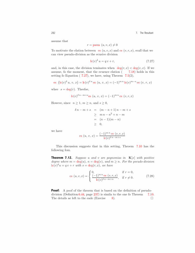
282 7. The Resultant
assume thatr = psrem(u, v, x) �= 0.
To motivate the relation between res(u, v, x) and res(v, r, x), recall that wecan view pseudo-division as the recursive division
lc(v)δ u = q v + r, (7.27)
and, in this case, the division terminates when deg(r, x) < deg(v, x). If weassume, for the moment, that the recurrence relation (7.18) holds in thissetting for Equation (7.27), we have, using Theorem 7.5(2),
res(lc(v)δ u, v, x
)= lc(v)δ n res(u, v, x) = (−1)mn lc(v)m−s res(v, r, x)
where s = deg(r). Therefore,
lc(v)δ n−m+sres(u, v, x) = (−1)mn res(v, r, x).However, since n ≥ 1, m ≥ n, and s ≥ 0,
δ n−m+ s = (m− n+ 1)n−m+ s
≥ mn− n2 + n−m
= (n− 1)(m− n)≥ 0,
we have
res(u, v, x) =(−1)mn res(v, r, x)
lc(v)δ n−m+s.
This discussion suggests that in this setting, Theorem 7.10 has thefollowing form.
Theorem 7.12. Suppose u and v are polynomials in K[x] with positivedegree where m = deg(u), n = deg(v), and m ≥ n. For the pseudo-divisionlc(v)δu = q v + r with s = deg(r, x), we have
res(u, v, x) =
0, if r = 0,(−1)mn res(v, r, x)
lc(v)δ n−m+n, if r �= 0. (7.28)
Proof: A proof of the theorem that is based on the definition of pseudo-division (Definition 6.44, page 237) is similar to the one for Theorem 7.10.The details are left to the reader (Exercise 8). �
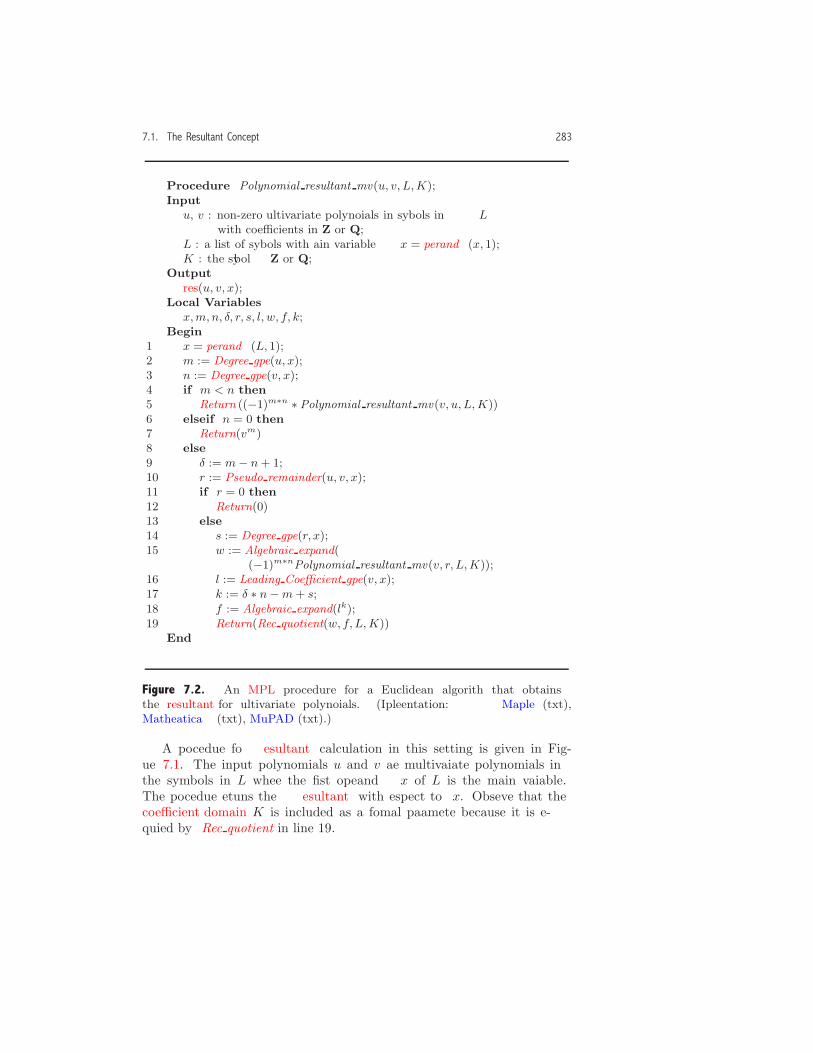
7.1. The Resultant Concept 283
Procedure Polynomial resultant mv(u, v, L,K);Input
u, v : non-zero multivariate polynomials in symbols in Lwith coefficients in Z or Q;
L : a list of symbols with main variable x = Operand(x, 1);K : the symbol Z or Q;
Outputres(u, v, x);
Local Variablesx,m, n, δ, r, s, l, w, f, k;
Begin1 x = Operand(L, 1);2 m := Degree gpe(u, x);3 n := Degree gpe(v, x);4 if m < n then5 Return ((−1)m∗n ∗ Polynomial resultant mv(v, u, L,K))6 elseif n = 0 then7 Return(vm)8 else9 δ := m− n + 1;10 r := Pseudo remainder(u, v, x);11 if r = 0 then12 Return(0)13 else14 s := Degree gpe(r, x);15 w := Algebraic expand(
(−1)m∗nPolynomial resultant mv(v, r, L,K));16 l := Leading Coefficient gpe(v, x);17 k := δ ∗ n−m + s;18 f := Algebraic expand(lk);19 Return(Rec quotient(w, f, L,K))
End
Figure 7.2. An MPL procedure for a Euclidean algorithm that obtainsthe resultant for multivariate polynomials. (Implementation: Maple (txt),Mathematica (txt), MuPAD (txt).)
A procedure for resultant calculation in this setting is given in Fig-ure 7.1. The input polynomials u and v are multivariate polynomials inthe symbols in L where the first operand x of L is the main variable.The procedure returns the resultant with respect to x. Observe that thecoefficient domain K is included as a formal parameter because it is re-quired by Rec quotient in line 19.

284 7. The Resultant
Recursive call deg(r, x) deg(r, y) Max. digitsr
1 4 4 42 3 10 63 2 22 144 1 54 33
Figure 7.3. Coefficient and degree explosion for the monomials in r obtained atline 10 in the procedure Polynomial resultant mv for the polynomials in Exam-ple 7.13.
Since Polynomial resultant and Polynomial resultant mv are based onpolynomial remainder sequences, they produce coefficient and degree ex-plosion similar to the gcd procedures in Figure 4.3 and Figure 6.6. Thispoint is illustrated in the next example.
Example 7.13. Consider the polynomials
u = x3y2 + 6 x4y + 9 x5 + 4 x2y2 + 24 x3y + 36 x4 + 5 xy2 + 30 yx2
+45 x3 + 2 y2 + 12 y x+ 18 x2,
v = x5y2 + 8 x4y + 16 x3 + 12 x4y2 + 96 x3y + 192 x2 + 45 x3y2
+360 yx2 + 720 x+ 50 x2y2 + 400 y x+ 800
as polynomials in Z[x, y] with x the main variable. In Example 6.63(page 250), we obtained gcd(u, v) = x+2, and, therefore, by Theorem 7.9,
res(u, v, x) = 0.
In Figure 7.3, we give a summary of the coefficient and degree explosion ob-tained in the monomials in the pseudo-remainder r at line 10 in Figure 7.1.Observe that there is a dramatic increase in the coefficient and degree ex-plosion for subsequent procedure calls. Eventually, the pseudo-remainderr = 0 terminates the recursion (lines 11–12), and so the recursion unwindsgiving a resultant of 0. �
Resultant Calculation: The Subresultant Remainder Sequence. There are a num-ber of ways to reduce the coefficient and degree explosion in resultant calculation.We briefly describe an approach based on the subresultant remainder se-quence that was used in Section 6.3 to reduce coefficient and degree explo-sion in multivariate gcd calculations. This approach involves the remaindersequence
S−1 = pp(u),

7.1. The Resultant Concept 285
Recursive call deg(r, x) deg(r, y) Max. digitsr
1 4 4 42 3 8 73 2 12 94 1 16 14
Figure 7.4. Coefficient and degree explosion for the monomials in r obtained atline 9 in the procedure Sr polynomial resultant rec for the polynomials in Exam-ples 7.13 and 7.14.
S0 = pp(v),
S1 =psrem(S−1, S0, x)
β1,
...
Si =psrem(Si−2, Si−1, x)
βi, (7.29)
...
which reduces the coefficient and degree explosion by dividing the pseudo-remainders by the expression βi given by the recurrence relations
ψ1 = −1, β1 = (−1)δ1 , (7.30)
ψi =(−lc(Si−2, x))δ(i−1)−1
ψδ(i−1)−2
i−1
, i > 1, (7.31)
βi = −lc(Si−2, x)ψδi−1i , i > 1 (7.32)
whereδi = deg(Si−2, x)− deg(Si−1, x) + 1, i ≥ 1. (7.33)
Procedures to compute the resultant using this approach are given inFigures 7.5, 7.6, and 7.7. The main procedure Sr polynomial resultantremoves the content of the polynomials and then obtains the resultant of theprimitive parts using the recursive procedure Sr polynomial resultant rec.At line 10, the resultant is obtained using Theorem 7.5(2),(3).
The recursive procedure Sr polynomial resultant rec performs the cal-culations using the subresultant remainder sequence. Observe that theformal parameter list includes δp and ψp which correspond to the previous
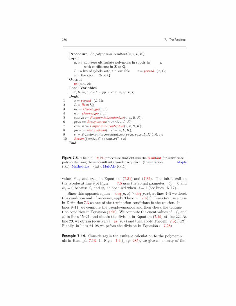
286 7. The Resultant
Procedure Sr polynomial resultant (u, v, L,K);Input
u, v : non-zero multivariate polynomials in symbols in Lwith coefficients in Z or Q;
L : a list of symbols with main variable x = Operand(x, 1);K : the symbol Z or Q;
Outputres(u, v, x);
Local Variablesx,R,m, n, cont u , pp u, cont v , pp v , s;
Begin1 x = Operand(L, 1);2 R = Rest(L);3 m := Degree gpe(u, x);4 n := Degree gpe(v, x);5 cont u := Polynomial content sr(u, x,R,K);6 pp u := Rec quotient(u, cont u, L,K);7 cont v := Polynomial content sr(v, x,R,K);8 pp v := Rec quotient(v, cont v , L,K);9 s := Sr polynomial resultant rec(pp u, pp v , L,K, 1, 0, 0);10 Return((cont u)n ∗ (cont v)m ∗ s)
End
Figure 7.5. The main MPL procedure that obtains the resultant for multivariatepolynomials using the subresultant remainder sequence. (Implementation: Maple(txt), Mathematica (txt), MuPAD (txt).)
values δi−1 and ψi−1 in Equations (7.31) and (7.32). The initial call onthe procedure at line 9 of Figure 7.5 uses the actual parameters δp = 0 andψp = 0 because δp and ψp are not used when i = 1 (see lines 15–17).
Since this approach requires deg(u, x) ≥ deg(v, x), at lines 4–5 we checkthis condition and, if necessary, apply Theorem 7.5(1). Lines 6-7 use a casein Definition 7.3 as one of the termination conditions for the recursion. Inlines 9–11, we compute the pseudo-remainder and then check the termina-tion condition in Equation (7.28). We compute the current values of ψi andβi in lines 15–21, and obtain the division in Equation (7.29) at line 22. Atline 23, we obtain (recursively) res(v, r) and then apply Theorem 7.5(1),(2).Finally, in lines 24–28 we perform the division in Equation (7.28).
Example 7.14. Consider again the resultant calculation for the polynomi-als in Example 7.13. In Figure 7.4 (page 285), we give a summary of the

7.1. The Resultant Concept 287
Procedure Sr polynomial resultant rec(u, v, L,K, i, δp, ψp);Input
u, v : non-zero multivariate polynomials in symbols in Lwith coefficients in Z or Q;
L : a list of symbols with main variable x = Operand(x, 1);K : the symbol Z or Q;i, δp, ψp : non-negative integers;
Outputres(u, v, x);
Local Variablesx,m, n, r, δ, R, ψ, β, f, s, w, l, k;
Begin1 x = Operand(L, 1);2 m := Degree gpe(u, x);3 n := Degree gpe(v, x);4 if m < n then5 Return((−1)m∗n ∗ Sr polynomial resultant rec(v, u, L,K, i, δp, ψp))6 elseif n = 0 then7 Return(vm)8 else9 r := Pseudo remainder(u, v, x);10 if r = 0 then11 Return(0)
Continued in Figure 7.7
Figure 7.6. A recursive MPL procedure that obtains the resultant for multivari-ate polynomials using the sub-resultant remainder sequence. (Implementation:Maple (txt), Mathematica (txt), MuPAD (txt).)
coefficient and degree explosion obtained in the monomials in the pseudo-remainder r at line 9 in the procedure Sr polynomial resultant rec in Fig-ure 7.6. Comparing these results with those in Figure 7.3, we see that sub-resultant remainder sequence significantly reduces degree and coefficientexplosion. �
Exercises1. Let u = x3 − 1 and v = x2 + 2.
(a) Give the Sylvester matrix S(u, v, x).
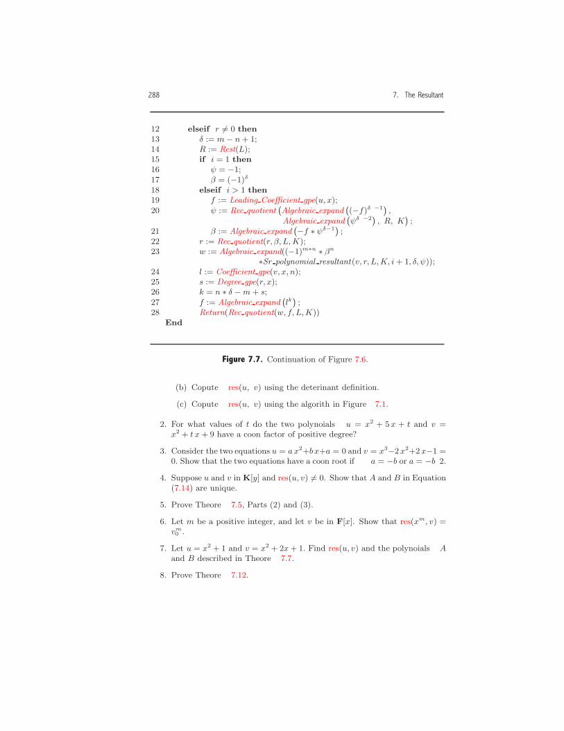
288 7. The Resultant
12 elseif r �= 0 then13 δ := m− n + 1;14 R := Rest(L);15 if i = 1 then16 ψ = −1;17 β = (−1)δ
18 elseif i > 1 then19 f := Leading Coefficient gpe(u, x);
20 ψ := Rec quotient Algebraic expand (−f)δp−1 ,
Algebraic expand ψδp−2 , R, K ;21 β := Algebraic expand −f ∗ ψδ−1 ;22 r := Rec quotient(r, β, L,K);23 w := Algebraic expand((−1)m∗n ∗ βn
∗Sr polynomial resultant(v, r, L,K, i + 1, δ, ψ));24 l := Coefficient gpe(v, x, n);25 s := Degree gpe(r, x);26 k = n ∗ δ −m + s;
27 f := Algebraic expand lk ;28 Return(Rec quotient(w, f, L,K))
End
Figure 7.7. Continuation of Figure 7.6.
(b) Compute res(u, v) using the determinant definition.
(c) Compute res(u, v) using the algorithm in Figure 7.1.
2. For what values of t do the two polynomials u = x2 + 5x + t and v =x2 + t x + 9 have a common factor of positive degree?
3. Consider the two equations u = ax2+b x+a = 0 and v = x3−2x2+2x−1 =0. Show that the two equations have a common root if a = −b or a = −b/2.
4. Suppose u and v in K[y] and res(u, v) �= 0. Show that A and B in Equation(7.14) are unique.
5. Prove Theorem 7.5, Parts (2) and (3).
6. Let m be a positive integer, and let v be in F[x]. Show that res(xm, v) =vm0 .
7. Let u = x2 + 1 and v = x2 + 2x + 1. Find res(u, v) and the polynomials Aand B described in Theorem 7.7.
8. Prove Theorem 7.12.

7.2. Polynomial Relations for Explicit Algebraic Numbers 289
7.2 Polynomial Relations for Explicit Algebraic Numbers
Let α be an explicit algebraic number. The algorithm described in thissection uses the resultant to find a non-zero polynomial u(x) in Q[x] thathas α as a root. The algorithm is based on the following theorem.
Theorem 7.15. Let v(x) and w(x) be polynomials in Q[x] with positivedegree, and suppose that v(α) = 0 and w(β) = 0. Then:
1. α+ β is a root of
u(x) = res(v(x − y), w(y), y) = 0.
2. αβ is a root of
u(x) = res(ym v(x/y), w(y), y) = 0
where m = deg(v(x), x).
3. If α �= 0, then α−1 is a root of
u(x) = res(x y − 1, v(y), y) = 0.
4. If a/b is a positive rational number in standard form, then αa/b is aroot of
u(x) = res(v(y), xb − ya, y) = 0.
Proof: To show (1), define the polynomial
f(y) = v(α+ β − y).
Since f(β) = v(α) = 0 and w(β) = 0, the polynomials f and w havea common root β, and Theorem 7.9 implies that res(f(y), w(y), y) = 0.Therefore,
u(α+ β) = res(v(α + β − y), w(y), y) = res(f(y), w(y), y) = 0.
The other statements in the theorem are proved in a similar way (Ex-ercise 2). �
As a consequence of Theorem 7.15, we have the following theorem.
Theorem 7.16. The algebraic numbers A are a field.

290 7. The Resultant
Proof: Theorem 7.15 shows that the algebraic numbers are closed underaddition (Axiom F-1) and multiplication (Axiom F-2), and that the multi-plicative inverse of a non-zero algebraic number is also an algebraic number(Axiom F-12). The remaining field properties follow because the algebraicnumbers are included in the field of complex numbers. �
In the next few examples, we show that by repeatedly applying Theo-rem 7.15 we obtain a polynomial that has a given explicit algebraic numberas a root.
Example 7.17. Consider the explicit algebraic number
α = 21/2 + 31/2 + 51/2.
The three radicals in the sum have minimal polynomials
p2(x) = x2 − 2, p3(x) = x2 − 3, p5(x) = x2 − 5.
Using Theorem 7.15(1), 21/2 + 31/2 is a root of
u(x) = res(p2(x− y), p3(y), y) = x4 − 10 x2 + 1.
Applying the theorem again, we have α is a root of
res(u(x− y), p5(y), y) = x8 − 40 x6 + 352 x4 − 960 x2 + 576.
Since this polynomial is monic and irrreducible, it is the minimal polynomialfor α. �
Example 7.18. Consider the explicit algebraic number
α =1√
2 +√3+
1√5 +√7.
From the last example, the polynomial u1(x) = x4−10 x2+1 has 21/2+31/2
as a root, and applying Theorem 7.15(3), we obtain
u2(x) = res(x y − 1, u1(y), y) = x4 − 10 x2 + 1
which has 1/(21/2 + 31/2) as a root. (Although u1 = u2 in this case,this is not generally true.) In a similar way, 1/(51/2 + 71/2) is a root ofu3(x) = 4 x4 − 24 x2 + 1. Applying Theorem 7.15(1), α is a root of
u4(x) = res(u2(x − y), u3(y), y)= 256 x16 − 16384 x14 + 363776 x12 − 3729408 x10
+ 18468704 x8 − 39450624 x6 + 23165264 x4
− 3909760 x2 + 46225.

7.2. Polynomial Relations for Explicit Algebraic Numbers 291
Since this polynomial is irrreducible in Q[x], (1/lc(u4)) · u4 is the minimalpolynomial for α. �
Example 7.19. Letα =√2√3 +√6.
Repeated application of Theorem 7.15 gives
u(x) = x8 − 48 x6 + 576 x4 = x4 (x2 − 24)2 (7.34)
which has α as a root. In this case, u(x) is reducible and the factors of ugive additional information about α. In a numerical sense, α can have upto eight different values that correspond to the sign interpretations of itsthree square root symbols
(±√2)(±
√3) ±
√6. (7.35)
These numerical values are indicated by the factors of the polynomial. Forexample, since x4 is a factor, there are four choices of signs where theexpression (7.35) simplifies to zero:
(+√2)(+
√3)−
√6, (+
√2)(−
√3) +
√6,
(−√2)(+
√3) +
√6, (−
√2)(−
√3)−
√6.
In addition, since (x2 − 24)2 is a factor, there are two choices of signswhere the expression (7.35) simplifies to +
√24 = 2(+
√6), and two choices
of signs where it simplifies to −√24 = 2(−√6).It is interesting to see what happens when Theorem 7.15(3) is applied
to u(x) in Equation (7.34) to find the polynomial associated with
1(±√2)(±√3) ± √6 , (7.36)
because, for some choices of signs, the denominator is 0. In this case weobtain
res(x y − 1, u(y), y) = res(x y − 1, y8 − 48 y6 + 576 y4, y)= 576 x4 − 48 x2 + 1= (24 x2 − 1)2
which has as its solutions the four expressions in (7.36) where the signsare chosen so that division by 0 does not occur. In Exercise 3, we give aresultant relation that shows why this is so. �
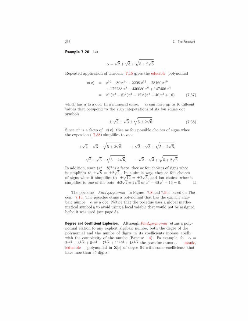
292 7. The Resultant
Example 7.20. Let
α =√2 +√3 +
√5 + 2
√6.
Repeated application of Theorem 7.15 gives the reducible polynomial
u(x) = x16 − 80 x14 + 2208 x12 − 28160 x10
+ 172288 x8 − 430080 x6 + 147456 x4
= x4 (x2 − 8)2(x2 − 12)2(x4 − 40 x2 + 16) (7.37)
which has α for a root. In a numerical sense, α can have up to 16 differentvalues that correspond to the sign interpretations of its four square rootsymbols
±√2±√3±
√5± 2
√6. (7.38)
Since x4 is a factor of u(x), there are four possible choices of signs wherethe expression (7.38) simplifies to zero:
+√2 +√3−
√5 + 2
√6, +
√2−√3 +
√5 + 2
√6,
−√2 +√3−
√5− 2
√6, −
√2−√3 +
√5 + 2
√6.
In addition, since (x2−8)2 is a factor, there are four choices of signs whereit simplifies to ±√8 = ±2√2. In a similar way, there are four choicesof signs where it simplifies to ±√12 = ±2√3, and four choices where itsimplifies to one of the roots ±2√2± 2
√3 of x4 − 40 x2 + 16 = 0. �
The procedure Find polynomial in Figures 7.8 and 7.9 is based on The-orem 7.15. The procedure returns a polynomial that has the explicit alge-braic number α as a root. Notice that the procedure uses a global mathe-matical symbol y to avoid using a local variable that would not be assignedbefore it was used (see page 3).
Degree and Coefficient Explosion. Although Find polynomial returns a poly-nomial relation for any explicit algebraic number, both the degree of thepolynomial and the number of digits in its coefficients increase rapidlywith the complexity of the number (Exercise 4). For example, for α =21/2 + 31/2 + 51/2 + 71/2 + 111/2 + 131/2 the procedure returns a monic,irrreducible polynomial in Z[x] of degree 64 with some coefficients thathave more than 35 digits.
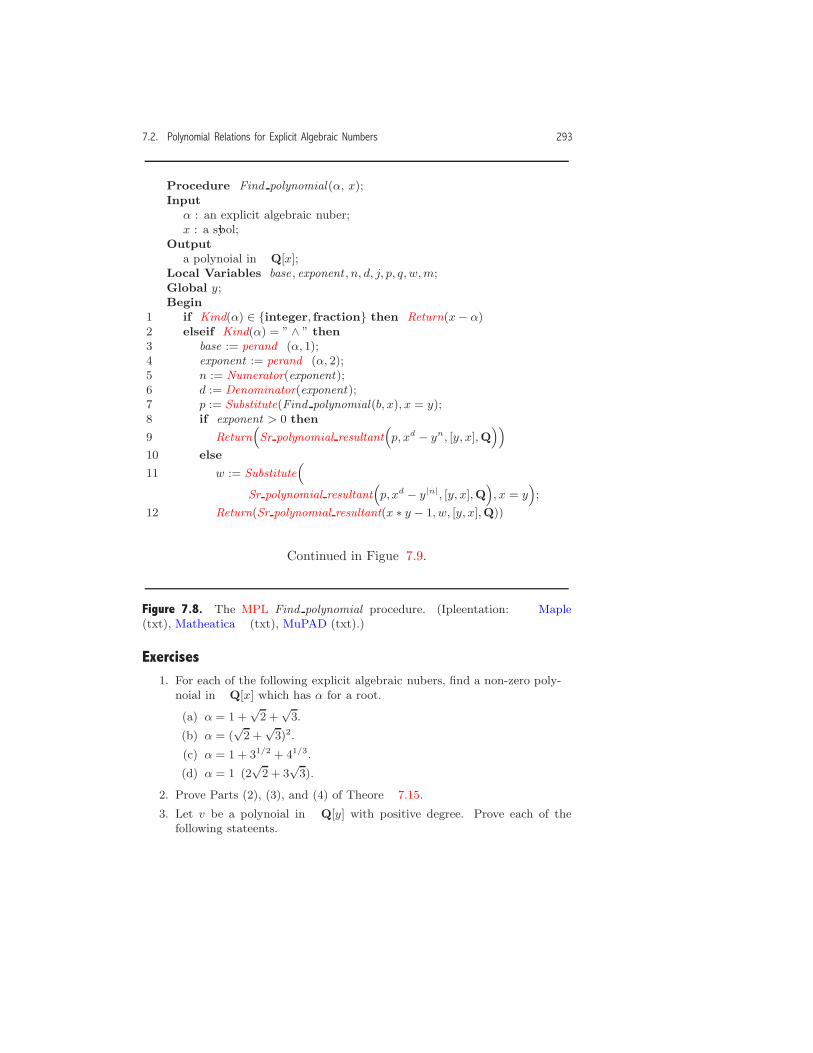
7.2. Polynomial Relations for Explicit Algebraic Numbers 293
Procedure Find polynomial(α, x);Input
α : an explicit algebraic number;x : a symbol;
Outputa polynomial in Q[x];
Local Variables base , exponent , n, d, j, p, q, w,m;Global y;Begin
1 if Kind(α) ∈ {integer, fraction} then Return(x− α)2 elseif Kind(α) = ” ∧ ” then3 base := Operand(α, 1);4 exponent := Operand(α, 2);5 n := Numerator(exponent);6 d := Denominator(exponent);7 p := Substitute(Find polynomial(b, x), x = y);8 if exponent > 0 then
9 Return Sr polynomial resultant p, xd − yn, [y, x],Q
10 else
11 w := Substitute
Sr polynomial resultant p, xd − y|n|, [y, x],Q , x = y ;
12 Return(Sr polynomial resultant(x ∗ y − 1, w, [y, x],Q))
Continued in Figure 7.9.
Figure 7.8. The MPL Find polynomial procedure. (Implementation: Maple(txt), Mathematica (txt), MuPAD (txt).)
Exercises1. For each of the following explicit algebraic numbers, find a non-zero poly-
nomial in Q[x] which has α for a root.
(a) α = 1 +√
2 +√
3.
(b) α = (√
2 +√
3)2.
(c) α = 1 + 31/2 + 41/3.
(d) α = 1/(2√
2 + 3√
3).
2. Prove Parts (2), (3), and (4) of Theorem 7.15.
3. Let v be a polynomial in Q[y] with positive degree. Prove each of thefollowing statements.

294 7. The Resultant
13 elseif Kind(α) = ” + ” then14 w := Find polynomial(Operand(α, 1), x);15 for j := 2 to Number of operands(α) do16 p := Find polynomial(Operand(α, j), x);17 q := Algebraic expand(Substitute(p, x = x− y));18 w := Sr polynomial resultant(q,Substitute(w, x = y), [y, x],Q);19 Return(w)20 elseif Kind(α) = ” ∗ ” then21 w := Find polynomial(Operand(α, 1), x);22 for j := 2 to Number of operands(α) do23 p := Find polynomial(Operand(α, j), x);24 m := Degree gpe(p, x);
25 q := Algebraic expand ym ∗ Substitute(p, x = x/y) ;
26 w := Sr polynomial resultant(q,Substitute(w, x = y), [y, x],Q);27 Return(w)
End
Figure 7.9. Continuation of Figure 7.8.
(a) If y|v(y), then res(x y − 1, v(y), y) = res(x y − 1, v(y)/y, y).
(b) Suppose that v(y) = 0 has zero as a root of multiplicity r. Show thatres(x y − 1, v(y), y) = res(x y − 1, v(y)/yr, y).
Notice that this exercise implies that if α �= 0 is a root of v(y) = 0, whichalso has zero as a root of multiplicity r, we can still apply the relation inTheorem 7.15 because the resultant is computed as if the factor yr (whichcorresponds to the root y = 0 of multiplicity r) has been removed.
4. In this exercise, we describe a way to find the degrees of the polyno-mials u(x) in Theorem 7.15. Let v and w be polynomials in F[x] withm = deg(v, x) > 0 and n = deg(w, x) > 0. Prove each of the followingstatements.
(a) deg(res(v(x− y), w(y), y), x) = mn.
(b) deg(res(ym v(x/y), w(y), y), x) = mn.
(c) If r is the maximum positive integer such that yr|v(y), then
deg(res(x y − 1, v(y), y), x) = m− r.
(d) If a/b is a positive rational number in standard form, then
deg(res(v(y), xb − ya, y), x) = bm.

7.2. Polynomial Relations for Explicit Algebraic Numbers 295
5. Suppose that α is a root of xm − 1 = 0 and β is a root of xn − 1 = 0. Showthat αβ is a root of xm n − 1.
6. Let α be an algebraic number which is a root of ax2 + b x+ c = 0, and letβ be an algebraic number which is a root of d x2 + e x + f = 0.
(a) Show that if c �= 0, then 1/α is a root of c x2 + b x + a = 0. (Thecondition c �= 0 implies that α �= 0.)
(b) Show that αβ is a root of
a2d2x4 − a b d e x3 + −2 a c d f + a e2 c + d b2f x2
−b c e f x + c2f2 = 0.
(c) Show that α + β is a root of
a2d2x4 + 2 a b d2 + 2 d e a2 x3
+ b2d2 + 2 d2a c + 3 a b d e + a2e2 + 2 a2d f x2
+ 2 a2e f + d e b2 + 2 a b d f + a e2b + 2 d2b c + 2 a c d e x
+ c2d2 + a b e f − 2 a c d f + a2f2 + f d b2 + a e2c + b c d e
= 0.
Further Reading
7.1 The Resultant Concept. See Akritas [2], Buchberger et al. [17] (“Com-puting in Algebraic Extensions”), Cohen [22], Geddes et al. [39], von zur Gathenand Gerhard [96], and Zippel [108] for a discussion of resultants. See Collins [26]for a discussion of the computation of multivariate polynomial resultants.
7.2 Polynomial Relations For Explicit Algebraic Numbers. The mate-
rial in this section is based on the work of R. Loos (see Buchberger et al. [17],
“Computing in Algebraic Extensions”).

8
Polynomial Simplificationwith Side Relations
In Section 4.3 we considered the simplification of polynomials with sym-bols for algebraic numbers that are defined as the solutions of polynomialequations. In Section 6.2 we considered the simplification of multivariatepolynomials with respect to a single polynomial side relation. In this chap-ter we again consider the polynomial simplification problem but this timeallow for several multivariate polynomial side relations that may have sym-bols in common. Because of this, the supporting mathematical theory ismore involved than the material in Sections 4.3 and 6.2. The algorithm inthis chapter is a generalization of the algorithms in these earlier sections.
In Section 8.1 we describe the division process that is used in the simpli-fication algorithm. In Section 8.2 we give a precise definition of the simpli-fication problem and introduce the concept of a Grobner basis which playsa key role in our algorithm. Finally, in Section 8.3, we give an algorithmthat finds a Grobner basis and the polynomial simplification algorithm.
8.1 Multiple Division and Reduction
To simplify the presentation, we assume that all polynomials are in thedomain Q[x1, . . . , xp]. We begin with some examples.
Example 8.1. Suppose that w, x, y, and z, satisfy the two side relations
f1 = w2 + x2 − 1 = 0, (8.1)
297
298 8. Polynomial Simplification with Side Relations
f2 = y z − 1 = 0, (8.2)
and consider the simplification of the polynomial
u =(y z2 + xw
)f1 + (w − z x) f2 (8.3)
= yz2 w2 + y z2 x2 − y z2 + xw3 + x3 w − xw + w y z
−w − z2 x y + z x (8.4)
with respect to the two side relations. Although it is evident from theunexpanded form in Equation (8.3) that u simplifies to 0 at all points thatsatisfy the side relations, this is not apparent from the expanded formin Equation (8.4). We can simplify the expanded form, however, usingmonomial-based division. First, dividing u by f1 and then using the siderelation f1 = 0, we obtain
u = mbquot(u, f1, [w, x]) f1 +mbrem(u, f1, [w, x])= mbrem(u, f1, [w, x])= w y z − w − z2 x y + z x
In a similar way, dividing the new u by f2 and then using the side relationf2 = 0, we obtain the simplified form for u
u = mbrem(u, f2, [y, z]) = 0.
In this example, since the two side relations are expressed in terms ofdifferent variables, we obtain the simplification with two division steps. �
The next example shows that the simplification problem is more in-volved when the two side relations have variables in common.
Example 8.2. Let x and y be solutions of the two side relations:
f1 = 3 x2 + 5x y − 5 x− 2 y2 + 11 y − 12 = 0, (8.5)f2 = 2 x2 + x y − 5 x− 3 y2 + 10 y − 7 = 0, (8.6)
and consider the simplification of the polynomial
u = x f1 + y f2 (8.7)= 3 x3 + 7 x2y − 5 x2 − x y2 + 6 x y − 12 x (8.8)−3 y3 + 10 y2 − 7y
with respect to these side relations. Again, it is evident from the unex-panded form in Equation (8.7) that u simplifies to 0, but not from theexpanded form in Equation (8.8).

8.1. Multiple Division and Reduction 299
Let’s try to obtain this simplification using monomial-based division.Dividing u by f1 with x as the main variable and then using the siderelation f1 = 0, we obtain
u = mbquot(u, f1, [x, y]) f1 +mbrem(u, f1, [x, y])= mbrem(u, f1, [x, y])
= −73x y2 − 5
3x y − 5
3y3 +
83y2 + y (8.9)
However, since lm(f2, [x, y]) = 2 x2 does not divide any monomial of uin Equation (8.9), division by f2 does not obtain the simplified form 0.Although we can continue the division process on u with y as the mainvariable, this again does not lead to the simplified form 0. In fact, nomatter how we order the divisions or the variables we cannot obtain thesimplified form 0 using monomial-based division.
The problem here is not so much with the division process but withthe form of the side relations. We shall see (in Section 8.3) that the firststep in our simplification algorithm is to obtain an equivalent set of siderelations (called the Grobner basis), and then to apply the division processwith these new side relations. In this case, the algorithm in Section 8.3gives the Grobner basis relations
g1 = 258 x+ 462 y3 − 1471 y2 + 339 y = 0, (8.10)g2 = 66 y4 − 163 y3 − 128 y2 + 217 y+ 116 = 0. (8.11)
Dividing u by g1 with x as the main variable, we obtain the remainder
r = −136959979507
y9 +26164677159014
y8 − 171536827318028
y7 +30264928275724504
y6
+37302171115724504
y5 − 80037712035724504
y4 +2405012995724504
y3
+12882318291431126
y2 − 1917572951431126
y − 137520262715563
,
and then division of r by g2 gives remainder 0. �
The goal in this chapter is the description of an algorithm that simplifiesa multivariate polynomial u with respect to the relations f1 = 0, . . . , fn =0. A precise description of this problem is given in Section 8.2, and thesimplification algorithm is given in Section 8.3.
Multiple Division
Let’s begin by examining in greater detail the division of a polynomial bya list of polynomial divisors. The condition in the next definition is usedto terminate the division process.

300 8. Polynomial Simplification with Side Relations
Definition 8.3. Let F be a set or list of non-zero distinct polynomialsf1, . . . , fn, and let L be a list of symbols . The polynomial u is reduced1
with respect to F if either u = 0 or if no monomial in u is divisible bylm(fi, L), i = 1, . . . , n.
This condition is similar to the one that terminates monomial-baseddivision with a single divisor (Definition 6.26, page 215). In Example 8.2above, Equation (8.9) is reduced with respect to the side relations in Equa-tions (8.5) and (8.6).
Definition 8.4. Let F = [f1, . . . , fn] be a list of non-zero polynomials, andlet L be a list of symbols that defines the variable order. Multiple divisionof a polynomial u by the divisor list F is defined by the iteration scheme:
c1 := c2 := · · · := cn := 0; r := u;
while r is not reduced with respect to F dofor i := 1 to n do
q := mbquot(r, fi, L);ci := ci + q;r := mbrem(r, fi, L);
The process terminates when r is reduced with respect to F . Upon termi-nation, the polynomials c1, . . . , cn are the multiple quotients with respectto F , and r is the multiple remainder.
Observe that the relations for q, ci, and r are defined (by assignments)in terms of the previous values of r and ci. The algorithm includes a forloop which is nested within a while loop. We have done this becausedivision by fj may introduce new opportunities for division by some otherfi with i < j, which means the process may require several passes throughthe while loop. (See Example 8.5 below and Exercise 2.) In addition, ateach division step in the for loop,
rold = qnew fi + rnew ,
where the rold is the old remainder value, and rnew and qnew are the newvalues. Therefore, since r = u at the start, at each iteration step we havethe representation
u = c1 f1 + · · ·+ cn fn + r (8.12)1Similar terms reducible and irrreducible were introduced to describe the factorization
of polynomials (Definition 4.11, page 118) and the factorization of expressions in anintegral domain (Definition 6.7, page 204). In this chapter the term reduced refers to theconcept in Definition 8.4.
8.1. Multiple Division and Reduction 301
where the polynomials ci and r are the most recently computed values. Attermination, the remainder r is reduced with respect to F .
The division process depends on both the order of the polynomials inF and the order of the symbols in L. This point is illustrated in the nextexample.
Example 8.5. Let
u = x3 + 2 x2y − 5 x+ y3 − 3 y, f1 = x y − 1, f2 = x2 + y2 − 4,
F = [f1, f2], and L = [x, y]. Monomial-based division of u by f1 gives
c1 = 0 + q = mbquot(u, f1, [x, y]) = 2 x,
r = mbrem(u, f1, [x, y]) = x3 − 3 x+ y3 − 3 y.
Next, division of r by f2 gives
c2 = 0 + q = mbquot(r, f2, [x, y]) = x,
r = mbrem(r, f2, [x, y]) = −x y2 + x+ y3 − 3 y.
Observe that division by f2 has created a new opportunity for division byf1. Division of r by f1 for a second time gives
c1 = 2 x+ q = 2 x+mbquot(r, f1, [x, y]) = 2 x− y,
r = mbrem(r, f1, [x, y]) = x+ y3 − 4 y.
Since r is reduced with respect to F , the process terminates, and we obtainthe representation for u in the form of Equation (8.12)
u = (2 x− y) f1 + x f2 + (x+ y3 − 4 y). (8.13)
The representation in Equation (8.12) is not unique. To obtain anotherrepresentation, we reverse the order of the divisions. Starting the processby dividing u by f2, we obtain
c2 = 0 + q = mbquot(u, f2, [x, y]) = x+ 2 y,
r = mbrem(u, f2, [x, y]) = −x y2 − x− y3 + 5 y,
and division of r by f1 gives
c1 = 0 + q = mbquot(r, f1, [x, y]) = −y,
r = mbrem(r, f1, [x, y]) = −x− y3 + 4 y.

302 8. Polynomial Simplification with Side Relations
Since r is reduced with respect to F , the division process terminates withanother representation
u = (−y) f1 + (x+ 2 y) f2 + (−x− y3 + 4 y). (8.14)
A third representation of the form in Equation (8.12) is obtained byusing y as the main variable and dividing u by [f1, f2]
u = x f1 + y f2 + (y + x3 − 4 x).
In this case, division of u by [f2, f1] with y as the main variable gives thesame representation. In fact, there are infinitely many representations ofthe form in Equation (8.12), although only three of them are obtained bymultiple division (Exercise 1). �
The properties of multiple division are given in the next theorem.
Theorem 8.6. Let u be a polynomial, F = [f1, . . . , fn] a list of non-zeropolynomials, and L a list of symbols that defines the variable order.
1. The multiple division algorithm terminates.
2. When the algorithm terminates,
u = c1f1 + · · ·+ cnfn + r (8.15)
where r is reduced with respect to F . In addition,
lm(r) �lm(u), (8.16)
and
lm(u)≡max ({lm(c1) lm(f1), . . . , lm(cn) lm(fn), lm(r)}) (8.17)
where the maximum is with respect to the monomial order relation.
Proof: Consider the algorithm in Definition 8.4. First, if u = 0, thealgorithm terminates immediately, and so we assume that u �= 0. After onepass through the while loop, the remainder r = R1 has the form
R1 = M1 + T1,
whereM1 is reduced with respect to F , and each monomial in T1 is divisibleby some lm(fi), i = 1, . . . , n− 1. (We have not included lm(fn) in this list
8.1. Multiple Division and Reduction 303
because after completing the for loop, R1 is reduced with respect to fn.)We show that
lm(T1)≺lm(u).
To see why, let t be a monomial of T1, and suppose that lm(fi)|t. How-ever, after division by fi, all monomials in the current remainder are notdivisible by lm(fi). Therefore, for some j > i, the operation mbrem(r, fj)has created a monomial s with the same variable part as t. By Theo-rem 6.30(2), at each step in the for loop, lm(r) �lm(u). In addition, byTheorem 6.28(8), s≺lm(r), and therefore lm(T1)≺lm(u).
Consider now the second pass through the while loop. Since M1 isreduced with respect to F , the termination of the process depends only onT1. Therefore, for the sake of analysis, let’s apply the division operationsto M1 and T1 separately.2 First, since M1 is reduced with respect to F ,the execution of the for loop beginning with r = M1 simply gives M1 fora remainder. Next, beginning with r = T1, the execution of the for loopgives a remainder M2+T2 where M2 is reduced with respect to F and eachmonomial in T2 is divisible by some lm(fi), i = 1, . . . , n − 1. Therefore,starting with r = M1 +T1, the execution of the for loop gives a remainder
R2 = M1 +M2 + T2.
In addition, using an argument similar to the one in the previous paragraph,we have
lm(T2)≺lm(T1).
In general, after s passes through the while loop, the remainder has theform
Rs = M1 + · · ·+Ms + Ts
where eachMi is reduced with respect to F , each monomial in Ts is divisibleby some lm(fi), i = 1, . . . , n− 1, and
lm(Ts)≺lm(Ts−1)≺ · · ·≺lm(T1)≺lm(u).Therefore, after some pass through the while loop, Ti = 0 and the processterminates.
To show (2), Equation (8.15) is given in Equation (8.12), and the re-duction (8.16) follows by repeatedly applying the relation (6.36) in Theo-rem 6.30 (page 220) at each monomial-based division step in the for loop.
For now, we omit the proof of Equation (8.17), because we prove it laterfor a more general division process called reduction. �
A procedure that performs multiple division is described in Exercise 3.2See Exercise 6 on page 228 for a justification for this approach.

304 8. Polynomial Simplification with Side Relations
Reduction
From an algorithmic perspective, multiple division is adequate for our sim-plification process as long as the side relations have the proper form. Froma theoretical (and practical) perspective, however, we need a more flexi-ble division process. The next two examples illustrate some limitations ofmultiple division.
Example 8.7. Let f1 = x y − 1, f2 = x2 + y2 − 4, L = [x, y], and
u = 2 x3 + 3 x2y + x2 + 2 y3 + 4 y + 1.
Using multiple division of u by F1 = [f1, f2], we obtain the representation
u = (3 x− 2 y) f1 + (2 x+ 1) f2 + r (8.18)
with remainderr = 11 x+ 2 y3 − y2 + 2 y + 5.
Next, let f3 = r, and consider the division of u by
F2 = [f1, f2, f3]. (8.19)
Since we have included the remainder r in F2, we might expect the remain-der in this division to be 0. Instead, we obtain the representation
u = 3 x f1 + (2 x+ 1) f2 +(− 211
y2 + 1)
f3 (8.20)
+(411
y5 − 211
y4 +411
y3 +1011
y2 + 2 y)
where the sum in parentheses on the last line is the non-zero remainder.The problem here is the division of u by F1 requires two passes throughthe while loop using the divisor sequence f1, f2, f1, f2. By including f3 inF2, multiple division uses the divisor sequence f1, f2, f3, f1, f2, f3 whichgives a non-zero remainder. In fact, no matter how we order the divisors inEquation (8.19), multiple division obtains a representation with a non-zeroremainder.
There is, however, a way to divide u by the set {f1, f2, f3} that obtainsthe remainder 0, although it doesn’t use the divisor sequence specified bythe for loop in Definition 8.4. In fact, if we perform division using thedivisor sequence
f1, f2, f1, f2, f3, (8.21)
we obtain the representation

8.1. Multiple Division and Reduction 305
u = (3 x− 2 y) f1 + (2 x+ 1) f2 + f3 (8.22)
which has remainder 0. �
Example 8.8. Let f1 = x y − 1, f2 = x2 + y2 − 4, L = [x, y], and
u = x2 + x y + y2 − 5.
Using multiple division of u by [f1, f2], we obtain the representation
u = f1 + f2 (8.23)
which has remainder 0. Consider next the division of
v =(x y2
)u = x3 y2 + x2 y3 + x y4 − 5 x y2 (8.24)
by [f1, f2]. Since we have simply multiplied u by the monomial x y2, wemight expect that this division also has remainder 0. Instead, we obtainthe representation
v = (x2 y + x y2 + x+ y3 − 4 y) f1 + 0 · f2 +(x+ y3 − 4 y
), (8.25)
where the sum in parentheses on the right is the non-zero remainder. Inaddition, reversing the order of the divisors does not help because divisionof v by [f2, f1] gives the representation
v = (−y) f1 + (y3 + x y2) f2 + (−y5 + 4 y3 − y) (8.26)
where again the sum in parentheses on the right is the non-zero remainder.In Example 8.16 below, we show how to obtain a remainder 0 for Equation(8.24) using another approach to division. �
In the previous two examples, we start with a division (Equations (8.18)and (8.23)), and then consider a related division where we would like (butdo not obtain) a remainder 0 (Equations (8.20) and (8.25)). Since weneed a division process that is flexible enough to obtain both of thesesimplifications, we consider another approach to division.
The new (and more general) division scheme must overcome two prob-lems with multiple division. First, as we saw in Example 8.7, the newprocess must have some flexibility in the choice of the order of the divi-sors. Next, as we saw in Example 8.8, simply reordering the divisors doesnot solve all of our problems. As we shall see in Example 8.16 below, theproblem here is that each monomial-based division step actually performstoo much simplification. For this reason, we need to change the individualdivision step as well as the order of the divisions.

306 8. Polynomial Simplification with Side Relations
The operation in the next definition replaces monomial-based divisionwith a simplified division process.
Definition 8.9. Let u and f �= 0 be polynomials, and let L be a list ofsymbols that defines the variable order. For m a monomial of u such thatlm(f)|m, the reduction step of u by f using the monomial m is given by
Q = m/lm(f),R = u−Qf.
The polynomial Q is the quotient of the reduction step, and R is its re-mainder. We use the notation
u[f,m]=⇒ R (8.27)
to indicate that the reduction step of u by f using the monomial m gives aremainder R.
The reduction step simplifies the process by applying only one step ofmonomial-based division to a single monomial m of u. Since
u = Qf +R, (8.28)
we view the reduction step as a form of division even though the remainderR may not be reduced with respect to the divisor f . Since a reduction stepis used to simplify u with respect to side relation f = 0, we have introducedthe notation in (8.27) as a way of indicating that the process simplifies uto R in the context of this side relation.
Example 8.10. Let
u = x3 y2 + x2 y3 + x y4 − 5 x y2, f = x2 + y2 − 4,
m = x3 y2, and L = [x, y]. Then, lm(f) = x2 and
Q = x3 y2/x2 = x y2, R = u−Qf = x2 y3 − x y2,
and so, u[f,m]=⇒ x2 y3 − x y2. �
The properties of a reduction step are given in the next theorem.
Theorem 8.11. Let u and f �= 0 be polynomials, and let L be a list ofsymbols that defines the variable order.

8.1. Multiple Division and Reduction 307
1. The remainder R in a reduction step of u by f with the monomial msatisfies lm(R) �lm(u).
2. If u �= 0 and m = lm(u), then lm(R)≺lm(u).3. lm(u)≡max({lm(Q) lm(f), lm(R)})
where the maximum is with respect to the monomial order relation.
Proof: To show (1), first, if u = 0, the inequality follows immediately fromthe definition. Next, suppose that u �= 0, and let f = lm(f) + fr where frrepresents the lower order monomials. Then
R = u− m
lm(f)f
= u− m
lm(f)lm(f)− m
lm(f)fr
= (u−m)−(
m
lm(f)fr
). (8.29)
Let’s consider the two expressions in parentheses. First,
lm(u−m) �lm(u). (8.30)
In addition,
lm(
m
lm(f)fr
)≺lm
(m
lm(f)lm(f)
)= m �lm(u). (8.31)
From Equation (8.29) and the relations (8.30) and (8.31), we have
lm(R) �max({
u− lm(u), lm(
m
lm(f)fr
)})�lm(u).
For Part (2), the proof is the same as Part (1) with the relation (8.30)replaced by lm(u− lm(u))≺lm(u).
To show (3), first, if u = 0, the relationship follows immediately fromthe definition. Next, if u �= 0 we have, using Equation (8.28),
lm(u) �max({lm(Q)lm(f), lm(R)}). (8.32)
In addition, by Part (1),
lm(Qf) = lm(u −R) �max({lm(u), lm(R)})≡lm(u). (8.33)
From Part (1) and the relation (8.33), we have
max({lm(Q)lm(f), lm(R)}) �lm(u). (8.34)

308 8. Polynomial Simplification with Side Relations
Therefore, the relations (8.32) and (8.34) imply that
lm(u)≡max({lm(Q)lm(f), lm(R)}). �
The new division process for a set of divisors is described in the nextdefinition.
Definition 8.12. Let F = {f1, . . . , fn} be a set of non-zero polynomials, andlet L be a list of symbols that defines the variable order. The reduction ofa polynomial u by the divisor set F is defined by the iteration scheme:
c1 := c2 := · · · := cn := 0; r := u;
while r is not reduced with respect to F doSelect a monomial m in r and a divisor fi in F
such that lm(fi, L)|m;Q := m/lm(fi, L);ci := ci +Q;r := r −Qfi;
The process terminates when r is reduced with respect to F . When this oc-curs, the polynomials c1, . . . , cn are the reduction quotients with respectto F , and r is the reduction remainder. We use the notation
uF−→ r (8.35)
to indicate that the reduction of u by F gives a remainder r.
Observe that each pass through thewhile loop involves a single reductionstep, and, for each step,
rold = Qnew fi + rnew ,
where rold is the old remainder value, and rnew and Qnew are the newvalues. Therefore, since r = u at the start, at each iteration step we obtainthe representation
u = c1 f1 + · · ·+ cn fn + r, (8.36)
where the polynomials ci and r are the most recently computed values. Attermination, the remainder r is reduced with respect to F .
Since the division process introduced here is used to simplify an expres-sion with respect to side relations f1 = 0, . . . , fn = 0, we have introduced

8.1. Multiple Division and Reduction 309
the notation in (8.35) as a way of indicating that the process simplifies u tor in the context of these side relations using some reduction step sequence
u = r0[fi1 ,m1]=⇒ r1
[fi2 ,m2]=⇒ · · · [fiq ,mq ]
=⇒ = rq = r. (8.37)
Keep in mind, however, if we chose another reduction step sequence, wemay obtain
uF−→ s
where s �= r.Of course, the process in Definition 8.12 is not really an algorithm until
we give a selection scheme for choosing the monomial m and the divisorfi. One possible scheme is multiple division (see Example 8.13 below), andanother one is given in Figure 8.1 below. For now, we assume that somescheme is given (which may vary from example to example) and the processterminates.
A reduction can be obtained with many different reduction step se-quences. This point is illustrated in the next example.
Example 8.13. Let
u = x3 + 2 x2 y − 5 x+ y3 − 3 y, f1 = x y − 1, f2 = x2 + y2 − 4,
where L = [x, y]. In Example 8.5 we considered the multiple division ofu by [f1, f2] which obtains the remainder x + y3 − 4 y using the divisorsequence f1, f2, f1 (see Equation (8.13)). From the reduction perspective,this division obtains
u{f1, f2}−→ x+ y3 − 4 y (8.38)
using the reduction step sequence
u[f1,2x
2y]=⇒ x3 − 3 x+ y3 − 3 y
[f2,x3]
=⇒ −x y2 + x+ y3 − 3 y (8.39)[f1,−x y2]=⇒ x+ y3 − 4 y.
We also obtain the reduction (8.38) using two other reduction step se-quences:
u[f2,x
3]=⇒ 2 x2 y − x y2 − x+ y3 − 3 y
[f1,2x2y]
=⇒ −x y2 + x+ y3 − 3y (8.40)[f1,−xy2]=⇒ x+ y3 − 4 y,

310 8. Polynomial Simplification with Side Relations
u[f2,x
3]=⇒ 2 x2 y − x y2 − x+ y3 − 3 y
[f1,−x y2]=⇒ 2 x2y − x+ y3 − 4 y (8.41)[f1,2 x
2y]=⇒ x+ y3 − 4 y,
although neither one of them is obtained by multiple division.In Example 8.5 we also considered the multiple division of u by [f2, f1],
which obtains the remainder −x−y3+4y using the divisor sequence f2, f1
(see Equation (8.14)). This division corresponds to the reduction
u{f1,f2}−→ − x− y3 + 4 y (8.42)
using the reduction step sequence
u[f2,2x
2y]=⇒ x3 − 5 x− y3 + 5 y
[f2,x3]
=⇒ −x y2 − x− y3 + 5 y (8.43)[f1,−x y2]=⇒ −x− y3 + 4 y.
In this case, the first two reduction steps correspond to monomial-baseddivision by f2, and the last step to monomial-based division by f1.
We can also obtain the reduction (8.42) using two other reduction stepsequences (Exercise 4). In fact, these six reduction step sequences are theonly ones possible with u, f1, and f2.
In Example 8.37 below, we show that u can be simplified to 0 withrespect to the side relations f1 = 0, f2 = 0, although this is not obtainedwith reduction by {f1, f2}. �
Example 8.14. Let f1 = x y − 1, f2 = x2 + y2 − 4, L = [x, y], and
u = 2x3 + 3x2y + x2 + 2y3 + 4y + 1.
In Example 8.7 we considered the multiple division of u by F1 = [f1, f2]which obtained the remainder 11x+2y3−y2+2y+5 (see Equation (8.18)).This corresponds to the reduction
u{f1,f2}−→ 11x+ 2y3 − y2 + 2y + 5 (8.44)
with reduction step sequence
u[f1,3x
2y]=⇒ 2x3 + x2 + 3x+ 2y3 + 4y + 1
[f2,2x3]
=⇒ x2 − 2x y2 + 11x+ 2y3 + 4y + 1 (8.45)

8.1. Multiple Division and Reduction 311
[f2,x2]
=⇒ 2 y3 + 4 y + 5 + 11 x− 2 xy2 − y2
[f1,−2x y2]=⇒ 11x+ 2y3 − y2 + 2y + 5.
We can also obtain the reduction (8.44) with 11 other reduction step se-quences, although none of them are obtained with multiple division. Inaddition, there are 12 reduction step sequences that reduce u to anotherpolynomial, one of which corresponds to multiple division by [f2, f1] (Ex-ercise 5).
Let f3 = 11x + 2y3 − y2 + 2y + 5 which is the polynomial obtainedwith the reduction (8.44). In Example 8.7 we observed that u could not bereduced to 0 using multiple division by the polynomials {f1, f2, f3} usingany divisor order. However, u
{f1,f2,f3}−→ 0 using the reduction step sequence(8.45) followed by the reduction step
11x+ 2y3 − y2 + 2y + 5[f3,11x]=⇒ 0. �
The next theorem, which plays a role in the implementation of ouralgorithm, describes the last reduction in the previous example.
Theorem 8.15. Let S = {f1, . . . , fn} be a set of non-zero polynomials, andlet L be a list of symbols that defines the variable order. Suppose that thereis a reduction step sequence which gives
uS−→ r, (8.46)
and let fn+1 = r and T = {f1, . . . , fn, fn+1}. Then there is a reductionstep sequence which gives
uT−→ 0. (8.47)
Proof: The reduction step sequence for (8.47) is simply the one used toobtain (8.46) followed by the reduction step
r[fn+1,lm(r)]
=⇒ 0. �
Example 8.16. Consider the reduction of u = x2+x y+y2−5 with respectto F = {f1, f2} = {x y − 1, x2 + y2 − 4} with L = [x, y]. In Example8.8 we showed that multiple division of u by [f1, f2] gives a representationwith remainder 0 (see Equation (8.23)). This division is obtained with thereduction step sequence
u[f1,x y]=⇒ (
x2 + y2 − 4) [f2,x
2]=⇒ 0. (8.48)

312 8. Polynomial Simplification with Side Relations
In Example 8.8 we also showed that multiple division of v = (x y2)u =x3y2 + x2y3 + x y4 − 5x y2 by [f1, f2] obtains remainder x + y3 − 4y (seeEquation (8.25)). This multiple division is obtained with the reductionstep sequence
v[f1,x
3 y2]=⇒ (
x2y3 + x2y + x y4 − 5x y2)
[f1,x2y3]
=⇒ (x2y + x y4 − 4x y2
)[f1,x
2y]=⇒ (
x y4 − 4x y2 + x)
[f1,x y4]
=⇒ (−4x y2 + x+ y3)
[f1,x]=⇒ (x+ y3 − 4y
).
Observe that multiple division has forced all reduction steps to be donewith f1. In other words, so much simplification is done by f1 there isnothing left to be done by f2. However, using a reduction step sequencesimilar to (8.48) we obtain
v[f1,x
2y3]=⇒ (
x3y2 + x y4 − x y2) [f2,x
3y2]=⇒ 0. (8.49)
In each case, the monomial used for reduction is the product of x y2 andthe corresponding monomial in (8.48). �
The next theorem, which plays an important role in the theoretical jus-tification of our algorithm, describes the relationship between the sequences(8.48) and (8.49).
Theorem 8.17. Let F = {f1, . . . , fn} be a set of non-zero polynomials, andlet L be a list of symbols that defines the variable order. Suppose that fora polynomial u, u F−→ g. Then, for a monomial m, mu
F−→mg.
Proof: Since uF−→ g, there is a sequence of reduction steps
u = r0[fi1 ,m1]=⇒ r1
[fi2 ,m2]=⇒ · · · [fiq ,mq]
=⇒ = rq = g.
whererj+1 = rj − mj
lm(fij )fij , j = 1, . . . , q.
Therefore,mrj+1 = mrj − mmj
lm(fij )fij ,

8.1. Multiple Division and Reduction 313
and
mu = mr0[fi1 ,mm1]=⇒ mr1
[fi2 ,mm2]=⇒ · · · [fiq ,mmq ]
=⇒ mrq = mg. �
The properties of the reduction process are given in the next theorem.
Theorem 8.18. Let u be a polynomial, F = [f1, . . . , fn] a list of non-zeropolynomials, and L a list of symbols that defines the variable order. Then,when reduction terminates
u = c1f1 + · · ·+ cnfn + r, (8.50)
lm(r) �lm(u), (8.51)
lm(u)≡max ({lm(c1)lm(f1), . . . , lm(cn)lm(fn), lm(r)}) (8.52)
where the maximum is with respect to the monomial order relation.
Proof: The representation (8.50) is given in Equation (8.36), and therelation (8.51) follows by applying Theorem 8.11(1) at each reduction stepin the process.
We show that Equation (8.52) holds at each reduction step using math-ematical induction. When the process begins,
c1 = 0, . . . , cn = 0, r = u.
At the first reduction step, for some fi in F , lm(fi)|lm(u) and
u = Qfi + r, ci = Q.
By Theorem 8.11(3),
lm(u)≡max({lm(Qfi), lm(r)}) = max({lm(ci)lm(fi), lm(r)}) (8.53)
which is Equation (8.52) at this point.For the induction step, we assume that Equation (8.52) holds at some
point in the process and show that it also holds at the next reduction step.Suppose that at this step
rnew = r −Qfi (8.54)
where rnew and Q are the most recently computed values. Since,
u = c1f1 + · · ·+ cnfn +Qfi + rnew
= c1f1 + · · ·+ ci−1fi−1 + (ci +Q)fi + ci+1fi+1 + · · ·+ cnfn + rnew ,
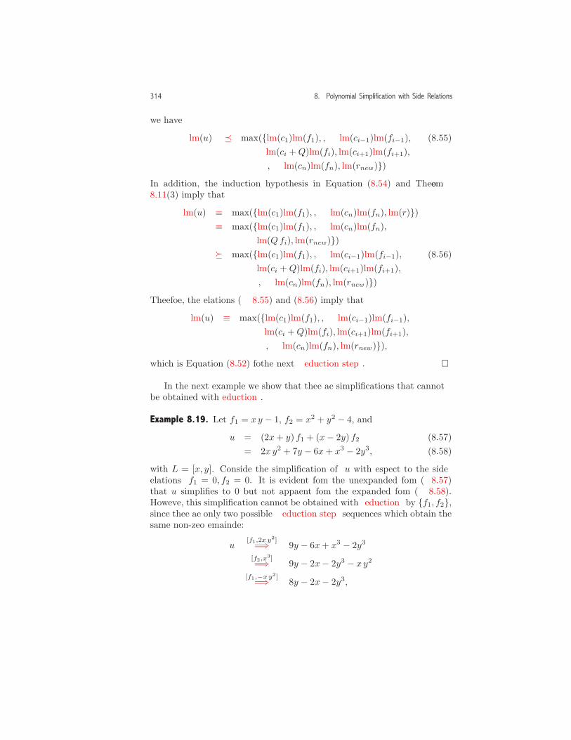
314 8. Polynomial Simplification with Side Relations
we have
lm(u) � max({lm(c1)lm(f1), . . . , lm(ci−1)lm(fi−1), (8.55)lm(ci +Q)lm(fi), lm(ci+1)lm(fi+1),. . . , lm(cn)lm(fn), lm(rnew )}).
In addition, the induction hypothesis in Equation (8.54) and Theorem8.11(3) imply that
lm(u) ≡ max({lm(c1)lm(f1), . . . , lm(cn)lm(fn), lm(r)})≡ max({lm(c1)lm(f1), . . . , lm(cn)lm(fn),
lm(Qfi), lm(rnew )})� max({lm(c1)lm(f1), . . . , lm(ci−1)lm(fi−1), (8.56)
lm(ci +Q)lm(fi), lm(ci+1)lm(fi+1),. . . , lm(cn)lm(fn), lm(rnew )}).
Therefore, the relations (8.55) and (8.56) imply that
lm(u) ≡ max({lm(c1)lm(f1), . . . , lm(ci−1)lm(fi−1),lm(ci +Q)lm(fi), lm(ci+1)lm(fi+1),. . . , lm(cn)lm(fn), lm(rnew )}),
which is Equation (8.52) for the next reduction step. �
In the next example we show that there are simplifications that cannotbe obtained with reduction.
Example 8.19. Let f1 = x y − 1, f2 = x2 + y2 − 4, and
u = (2x+ y) f1 + (x− 2y) f2 (8.57)= 2x y2 + 7y − 6x+ x3 − 2y3, (8.58)
with L = [x, y]. Consider the simplification of u with respect to the siderelations f1 = 0, f2 = 0. It is evident from the unexpanded form (8.57)that u simplifies to 0 but not apparent from the expanded form (8.58).However, this simplification cannot be obtained with reduction by {f1, f2},since there are only two possible reduction step sequences which obtain thesame non-zero remainder:
u[f1,2x y
2]=⇒ 9y − 6x+ x3 − 2y3
[f2,x3]
=⇒ 9y − 2x− 2y3 − x y2
[f1,−x y2]=⇒ 8y − 2x− 2y3,

8.1. Multiple Division and Reduction 315
u[f2,x
3]=⇒ x y2 + 7y − 2x− 2y3
[f1,x y2]
=⇒ 8y − 2x− 2y3.
The problem here is not the reduction process, but the form of the siderelations. In Example 8.37 (page 327) we show how this simplification isobtained using reduction with an equivalent set of side relations called theGrobner basis. �
Reduction AlgorithmIn Figure 8.1 we give a procedure Reduction that reduces u with respect toF using a selection scheme which obtains the reduction in Theorem 8.15.In this approach the current remainder is a sum r + R, where r containsmonomials that cannot be reduced by F , and R contains monomials thatmay be reducible. By doing this we can check for termination by sim-ply comparing R to 0 instead of checking whether the full remainder isreduced with respect to F , as is done in Definition 8.12. These variablesare initialized in lines 1–2.
At each pass through the while loop, we try to reduce R using areduction step with monomial m = lm(R) and a polynomial f from F .The divisibility test is given in line 11. Since a successful division at line10 results in a monomial which may have a coefficient that is an integer orfraction, we check for this by checking if the denominator of Q is an inte-ger. If the test is successful, we perform the reduction (line 12), update thequotient (line 13), and then continue the process with the first polynomialin F (line 14). By always returning to the first divisor after a successfulreduction, we insure that the selection scheme obtains the reduction inTheorem 8.15.
If the test at line 11 fails, we try again with the next divisor in thelist (line 16). However, if i is larger than the number of polynomials inF , the current monomial m is not divisible by the leading monomial ofany polynomial in F , and so it is removed from R (line 18), added to r(line 19), and the process repeats with the first polynomial in F (line 20).Lines 22-23 are included so that the quotients are returned in the list q.
Theorem 8.20. Let u be a polynomial, F = [f1, . . . fn] be a list of non-zero polynomials, and L be a list of symbols that defines the variable order.Then, the reduction algorithm in Figure 8.1 terminates.
Proof: By Theorem 8.11(2), at each execution of line 12, lm(R) decreaseswith respect to the ≺ relation. On the other hand, if lm(f) /| lm(R)for all polynomials f in F , then line 18 is executed and again lm(R) de-
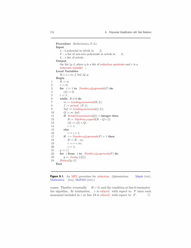
316 8. Polynomial Simplification with Side Relations
Procedure Reduction(u, F, L);Input
u : a polynomial in symbols in L;F : a list of non-zero polynomials in symbols in L;L : a list of symbols;
Outputthe list [q, r] where q is a list of reduction quotients and r is areduction remainder;
Local VariablesR, r, i, c,m, f, lmf , Q, q;
Begin1 R := u;2 r := 0;3 for i := 1 to Number of operands(F ) do4 c[i] := 0;5 i := 1;6 while R �= 0 do7 m := Leading monomial(R,L);8 f := Operand(F, i);9 lmf := Leading monomial(f, L);10 Q := m/lmf ;11 if Kind(Denominator(Q)) = integer then12 R := Algebraic expand(R−Q ∗ f);13 c[i] := c[i] + Q;14 i := 115 else16 i := i + 1;17 if i = Number of operands(F ) + 1 then18 R := R−m;19 r := r + m;20 i := 1;21 q := [ ];22 for i from 1 to Number of operands(F ) do23 q := Join(q, [c[i]]);24 Return([q, r])
End
Figure 8.1. An MPL procedure for reduction. (Implementation: Maple (txt),Mathematica (txt), MuPAD (txt).)
creases. Therefore, eventually R = 0, and the condition at line 6 terminatesthe algorithm. At termination, r is reduced with respect to F since eachmonomial included in r at line 19 is reduced with respect to F . �
8.1. Multiple Division and Reduction 317
The motivation for introducing the reduction process is to have a di-vision process that is flexible enough to obtain the reductions mentionedin Theorems 8.15 and 8.17. Although the Reduction procedure obtains thereduction in Theorem 8.15, it may not obtain the reduction in Theorem8.17. While Theorem 8.17 is of theoretical importance for the verificationof our simplification algorithm, it does not appear as a computational stepin the algorithm. For this reason, it is enough to know that the generalreduction process in Definition 8.12 can obtain this reduction, even thoughit is not obtained by the selection scheme used for the procedure Reduction.
Exercises1. Let u = x3 + 2x2y− 5x+ y3 − 3y, f1 = x y− 1 and f2 = x2 + y2 − 4, where
x is the main variable. Show that there are infinitely many representationsof u of the form (8.12). Hint: Find a general representation that containsEquations (8.13) and (8.14).
2. Let u = x y z + x z2 − x + y3 + y2 − y z2 + y − 1, and let
f1 = z2 − 1, f2 = y2 + y − z2, f3 = x z − y.
Show that u simplifies to 0 using the side relations f1 = 0, f2 = 0, f3 = 0.Note: This simplification requires three passes through the while loop inthe multiple division process in Definition 8.4.
3. Let u be a polynomial, F a list of non-zero polynomials, and let L be a listof variables that defines the variable order. Give a procedure
Multiple division(u, F, L)
that returns a two element list that contains the list of multiple quotientsand the multiple remainder.
4. Let
u = x3 + 2x2y − 5x + y3 − 3y, f1 = x y − 1, f2 = x2 + y2 − 4,
where L = [x, y].
(a) In Example 8.13 we gave a reduction step sequence for
u{f1,f2}−→ − x− y3 + 4y.
Find two more reduction step sequences that obtain this reduction.
(b) Show that there are six reduction step sequences for u with {f1, f2}.
5. Let f1 = x y − 1, f2 = x2 + y2 − 4, L = [x, y], and
u = 2x3 + 3x2y + x2 + 2y3 + 4y + 1.
318 8. Polynomial Simplification with Side Relations
(a) In Example 8.14 we gave a reduction sequence that obtains
u{f1,f2}−→ 11x + 2y3 − y2 + 2y + 5.
Find two more reduction step sequences that obtain this reduction.
(b) Find a reduction step sequence that reduces u to another polynomialusing {f1, f2}.
6. Let F = {f1, f2} = {x y − 1, x2 + y2 − 4} and L = [x, y]. For
u = x3 + 3x2y − 3y3,
find all possible reduction step sequences and indicate which ones corre-spond to a multiple division and which ones correspond to the algorithmin Figure 8.1.
8.2 Equivalence, Simplification, and Ideals
Let’s return now to our main goal, the development of a simplificationalgorithm that transforms a polynomial u to an equivalent polynomial vthat is simplified with respect to the side relations
f1 = 0, . . . , fn = 0. (8.59)
Polynomial Equivalence with Side Relations
Since simplification involves finding an equivalent simplified expression, webegin by addressing the meaning of equivalence.
Definition 8.21. Let u and v be polynomials, and let F = {f1, . . . , fn}be a set of non-zero polynomials in Q[x1, . . . , xp]. The polynomial u isequivalent to v with respect to the side relations (8.59) if
u(a1, . . . , ap) = v(a1, . . . , ap)
at each point (x1, . . . , xp) = (a1, . . . , ap) that is a solution of the system(8.59). (The values ai can be real or complex.) We use the notation
uF= v
to indicate that u is equivalent to v.
In other words, since the system of equations (8.59) defines a set ofpoints, two polynomials u and v are equivalent if they have the same valueas functions at each point in the solution set.

8.2. Equivalence, Simplification, and Ideals 319
Example 8.22. In Example 8.19 on page 314 we considered the simplifica-tion of
u = 2x y2 + 7y − 6x+ x3 − 2y3
with respect to the side relations
f1 = x y − 1 = 0, f2 = x2 + y2 − 4 = 0.
These equations have the four solutions
x = −(1/2√6 + 1/2
√2)3
+ 2√6 + 2
√2, y = 1/2
√6 + 1/2
√2,
x = −(1/2√6− 1/2
√2)3
− 2√6 + 2
√2, y = 1/2
√6− 1/2
√2,
x = −(−1/2
√6 + 1/2
√2)3
+ 2√6− 2
√2, y = −1/2
√6 + 1/2
√2,
x = −(−1/2√6− 1/2
√2)3
− 2√6− 2
√2, y = −1/2√6− 1/2
√2.
Since u evaluates to 0 at each of these points, we have uF=0. �
Consistent Side Relations
Polynomial equivalence is only meaningful if the system (8.59) has at leastone solution. This point is illustrated in the next example.
Example 8.23. Consider the side relations
f1 = x y + x+ 2y + 3 = 0, (8.60)
f2 = x y + 2y + 1 = 0. (8.61)
with F = {f1, f2}. This system of equations does not have a solution for xand y in the complex numbers. To see why, first eliminate y by subtractingEquation (8.61) from Equation (8.60) which gives x = −2. Substitutingthis value into Equation (8.60) gives 1 = 0, and so the system does nothave a solution.
In this situation equivalence is not meaningful because, in a trivialsense, any two polynomials are equivalent. In fact, 0 F=1 because thesetwo constant polynomials agree as functions at each point of the emptysolution set. �
In order that our simplification problem be meaningful, we assume thatour side relation equations are consistent in the following sense.

320 8. Polynomial Simplification with Side Relations
Definition 8.24. A system of equations f1 = 0, . . . , fn = 0 that has at leastone solution is called a consistent system of equations. If the system doesnot have a solution it is called an inconsistent system.
In Section 8.3 we show how to test for the consistency of the side rela-tions.
Equivalence and Reduction
Although Definition 8.21 is useful in a theoretical sense, it is not usefulin an algorithmic sense. First, consistent systems of equations may haveeither finitely many or infinitely many solutions. In addition, in most casesit is impossible to find a formula representations for solutions, and evenin cases where formulas are available, the verification of equivalence caninvolve a difficult radical simplification.
A better approach is to avoid the solution of the side relation equa-tions altogether. The next theorem suggests a more fruitful approach thatinvolves reduction.
Theorem 8.25. Let u and r be polynomials, F = {f1, . . . , fn} a set ofnon-zero polynomials, and L a list that determines variable order. Then,uF−→ r implies that u F= r.
Proof: Since uF−→ r, the polynomial u has a representation
u = c1f1 + · · · cnfn + r. (8.62)
For each point (x1, . . . , xp) = (a1, . . . , ap) in the solution set of
f1 = 0, . . . , fn = 0,
we have
u(a1, . . . , ap) = c1(a1, . . . , ap)f1(a1, . . . , ap) + · · ·+cn(a1, . . . , ap)fn(a1, . . . , ap) + r(a1, . . . , ap)
= r(a1, . . . , ap). �
This theorem suggests that instead of testing equivalence directly, wemight use reduction to test for equivalence. Unfortunately, something islost in the translation, since, as we saw in Example 8.19 (page 314), u F= r
does not imply that u F−→ r.
8.2. Equivalence, Simplification, and Ideals 321
The Zero Equivalence Problem
One aspect of simplification has to do with the zero equivalence problemwhich involves checking whether or not
uF=0. (8.63)
An important class of polynomials that satisfy Equation (8.63) consists ofthose polynomials that have a representation of the form
u = c1f1 + · · ·+ cnfn (8.64)
where c1, . . . , cn are polynomials in Q[x1, . . . , xp]. For this class of poly-
nomials, reduction can determine that uF=0 although this involves first
finding an equivalent set of side relations (the Grobner basis), and then ap-plying reduction with this new basis. (See Theorem 8.33(b) on page 325.)Unfortunately, there are polynomials that are equivalent to 0 that do nothave the form (8.64) for which reduction with a Grobner basis does notobtain 0. (See Theorem 8.58 on page 345 and Example 8.57 on page 345.)
The Goal of the Simplification Algorithm
In light of the previous discussion, we give two goals for our simplificationalgorithm.
1. If u has a representation of the form (8.64), the algorithm determines(using reduction) that u F=0. In addition, we require that this prop-erty does not depend on either the order in the symbol list L or theselection scheme used for reduction.
2. For polynomials u in Q[x1, . . . , xp] that do not have a representa-tion of the form (8.64), the algorithm obtains (using reduction) apolynomial r that is reduced with respect of F such that u F= r.
In order to describe the algorithm, we introduce some new terminologyand theoretical concepts.
Ideals
The collection of polynomials of the form (8.64) is referred to by the ter-minology in the next definition.
Definition 8.26. LetF = {f1, . . . , fn}

322 8. Polynomial Simplification with Side Relations
be a set of non-zero polynomials. The ideal I generated by F is the set ofpolynomials of the form
u = c1f1 + · · ·+ cnfn, (8.65)
where c1, . . . , cn are polynomials in Q[x1, . . . , xp]. The set F is called abasis for I, and the notation
I = < f1, . . . , fn >
indicates that I is generated by the basis.
In other words, one goal of the simplification algorithm is to obtain thesimplified form 0 for all polynomials in the ideal I = <f1, . . . , fn>.
The next theorem describes the basic algebraic properties of an ideal.
Theorem 8.27. Let I be an ideal with basis F = {f1, . . . , fn}.1. If u and v are in I, then u+ v is in I.
2. If u is in I and c is in Q[x1, . . . , xp], then c u is in I.
3. Suppose that u and v �= 0 are in I, and suppose that m is a monomial
of u with lm(v)|m. Then, u[v,m]=⇒ r implies that r is in I.
4. If u is in I and uF−→ r, then r is in I.
Proof: The proof of Parts (1) and (2) follow directly from the definitionof an ideal. The proof of Part (3) follows from the definition of a reductionstep together with Parts (1) and (2), and Part (4) follows from (3). Thedetails of the proofs are left to the reader (Exercise 2). �
Example 8.28. Consider the ideal I = <x + y, x − y > which consists ofall polynomials of the form
u(x, y) = c1(x + y) + c2(x− y) (8.66)
where c1 and c2 are polynomials. For example, the polynomial x2+y2 is inI with c1 = x and c2 = −y. The representation (8.66) is not unique sincec1 = y and c2 = x gives another representation for x2 + y2.
An ideal can have many different bases. For example, {x, y} is also abasis for I. To show this, we show that the set of polynomials of the form
u(x, y) = d1x+ d2y (8.67)

8.2. Equivalence, Simplification, and Ideals 323
is the same as the set of polynomials of the form (8.66). First, since
c1(x+ y) + c2(x− y) = (c1 + c2)x+ (c1 − c2) y,
any polynomial of the form (8.66) has the form (8.67). Conversely, since
d1x+ d2y =d1 + d2
2(x+ y) +
d1 − d2
2(x− y),
any polynomial of the form (8.67) has the form (8.66).Using the basis {x, y}, we can obtain another simple description of this
ideal. From Equation (8.67), u(0, 0) = 0, and so, each polynomial in Ihas a zero constant term. Conversely, any polynomial with zero constantterm is in I. To show this, suppose that u has a zero constant term,and consider the representation u = q x + r where q = mbquot(u, x) andr = mbrem(u, x). Notice that q x is the sum of all monomials in u thathave x as a factor, and r can depend on y but is free of x. Then, since
u(0, 0) = 0 = q(0, 0) · 0 + r(0),
we have r(0) = 0, which means that r has a zero constant term. Therefore,r = y s(y), and u has the required representation q x+ s y. �
In the next example, we show that for single variable polynomials, idealstake a particularly simple form.
Example 8.29. Consider an ideal I = <f1, . . . , fn> in Q[x] . Let f �= 0 bea polynomial in the ideal of minimal degree. We show that {f} is anotherbasis for the ideal. For any polynomial u in I, polynomial division of u byf gives u = q f + r where deg(r) < deg(f). However, since r = u− q f is inthe ideal, the minimal degree property of f implies that r = 0. Therefore,u = q f which means f is a basis for the ideal. In fact, it can be shownthat I = <gcd(f1, . . . , fn)> (Exercise 3(b)). �
An ideal with a single polynomial for a basis is called a principal ideal.The previous example shows that for single variable polynomials, all idealsare principal ideals. For polynomials with more than one variable, however,there are ideals that are not principal (Exercise 4).
Grobner Bases for IdealsReduction with respect to an ideal basis F may not obtain the remainder 0for polynomials in the ideal. However, if the basis is a special type knownas a Grobner basis,3 reduction does obtain the remainder 0.
3Grobner bases for ideals were invented by Bruno Buchberger who called themGrobner bases in honor of his Ph.D. dissertation advisor Wolfgang Grobner. Thesebases are also known as standard bases.

324 8. Polynomial Simplification with Side Relations
Definition 8.30. Let F = {f1, . . . , fn} be a set of non-zero polynomials,and suppose that I = < f1, . . . , fn >. The set F is a Grobner basis forI if for each u in I, there is an fi such that lm(fi)|lm(u).
Example 8.31. Consider the ideal I = <x+y, x−y> which was consideredin Example 8.28, and assume that L = [x, y].
We show first that F = {f1, f2} = {x+ y, x− y} is not a Grobner basisfor I. To see why, consider the polynomial
u = 2 y = f1 − f2
which is in I. Since both lm(f1, L) = x and lm(f2, L) = x do not dividelm(y, L) = y, F is not a Grobner basis.
However, G = {g1, g2} = {x, y} is a Grobner basis for the ideal. Toshow that G satisfies the Grobner basis property, from Example 8.28, Iconsists of all polynomials in x and y that do not have a constant term.Therefore, either lm(g1, L) = x or lm(g2, L) = y divides the leading mono-mial of each polynomial in I.
A similar argument shows that {x− y, 2y} is also a Grobner basis forI, and so, the Grobner basis is not unique. �
Example 8.32. Consider the ideal
I = <f1, f2> = <xy − 1, x2 + y2 − 4>
with L = [x, y]. We show that F = {f1, f2} is not a Grobner basis for I.Let
u = x+ y3 − 4y = −x f1 + y f2.
Observe that both lm(f1) = x y and lm(f2) = x2 do not divide lm(u) = x,and, therefore, F is not a Grobner basis.
A Grobner basis for this ideal is
G = {g1, g2} = {−y3 + 4y − x, y4 − 4y2 + 1}.First, since
f1 = −y g1 − g2, f2 = (−x+ y3 − 4y)g1 + (y2 − 4)g2,
andg1 = x f1 − y f2, g2 = (−x y + 1)f1 + y2f2,
G is also a basis for the ideal.Next, let
u = c1 g1 + c2 g2 = c1(−y3 + 4y − x) + c2(−y4 + 4y2 − 1)
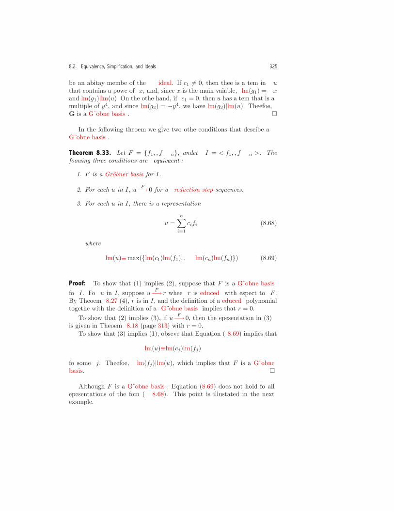
8.2. Equivalence, Simplification, and Ideals 325
be an arbitrary member of the ideal. If c1 �= 0, then there is a term in uthat contains a power of x, and, since x is the main variable, lm(g1) = −xand lm(g1)|lm(u). On the other hand, if c1 = 0, then u has a term that is amultiple of y4, and since lm(g2) = −y4, we have lm(g2)|lm(u). Therefore,G is a Grobner basis. �
In the following theorem we give two other conditions that describe aGrobner basis.
Theorem 8.33. Let F = {f1, . . . , fn}, and let I = < f1, . . . , fn >. Thefollowing three conditions are equivalent:
1. F is a Grobner basis for I.
2. For each u in I, u F−→ 0 for all reduction step sequences.
3. For each u in I, there is a representation
u =n∑i=1
cifi (8.68)
where
lm(u)≡max({lm(c1)lm(f1), . . . , lm(cn)lm(fn)}). (8.69)
Proof: To show that (1) implies (2), suppose that F is a Grobner basisfor I. For u in I, suppose u
F−→ r where r is reduced with respect to F .By Theorem 8.27 (4), r is in I, and the definition of a reduced polynomialtogether with the definition of a Grobner basis implies that r = 0.
To show that (2) implies (3), if u F−→ 0, then the representation in (3)is given in Theorem 8.18 (page 313) with r = 0.
To show that (3) implies (1), observe that Equation (8.69) implies that
lm(u)≡lm(cj)lm(fj)
for some j. Therefore, lm(fj)|lm(u), which implies that F is a Grobnerbasis. �
Although F is a Grobner basis, Equation (8.69) does not hold for allrepresentations of the form (8.68). This point is illustrated in the nextexample.
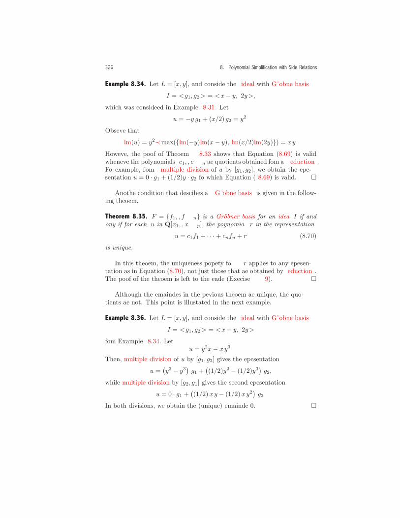
326 8. Polynomial Simplification with Side Relations
Example 8.34. Let L = [x, y], and consider the ideal with Grobner basis
I = <g1, g2> = <x− y, 2y>,
which was considered in Example 8.31. Let
u = −y g1 + (x/2) g2 = y2.
Observe that
lm(u) = y2≺max({lm(−y)lm(x− y), lm(x/2)lm(2y)}) = x y.
However, the proof of Theorem 8.33 shows that Equation (8.69) is validwhenever the polynomials c1, . . . , cn are quotients obtained from a reduction.For example, from multiple division of u by [g1, g2], we obtain the repre-sentation u = 0 · g1 + (1/2)y · g2 for which Equation (8.69) is valid. �
Another condition that describes a Grobner basis is given in the follow-ing theorem.
Theorem 8.35. F = {f1, . . . , fn} is a Grobner basis for an ideal I if andonly if for each u in Q[x1, . . . , xp], the polynomial r in the representation
u = c1f1 + · · ·+ cnfn + r (8.70)
is unique.
In this theorem, the uniqueness property for r applies to any represen-tation as in Equation (8.70), not just those that are obtained by reduction.The proof of the theorem is left to the reader (Exercise 9). �
Although the remainders in the previous theorem are unique, the quo-tients are not. This point is illustrated in the next example.
Example 8.36. Let L = [x, y], and consider the ideal with Grobner basis
I = <g1, g2> = <x− y, 2y>
from Example 8.34. Letu = y2x− x y3.
Then, multiple division of u by [g1, g2] gives the representation
u =(y2 − y3
)g1 +
((1/2)y2 − (1/2)y3
)g2,
while multiple division by [g2, g1] gives the second representation
u = 0 · g1 +((1/2)x y − (1/2)x y2
)g2.
In both divisions, we obtain the (unique) remainder 0. �
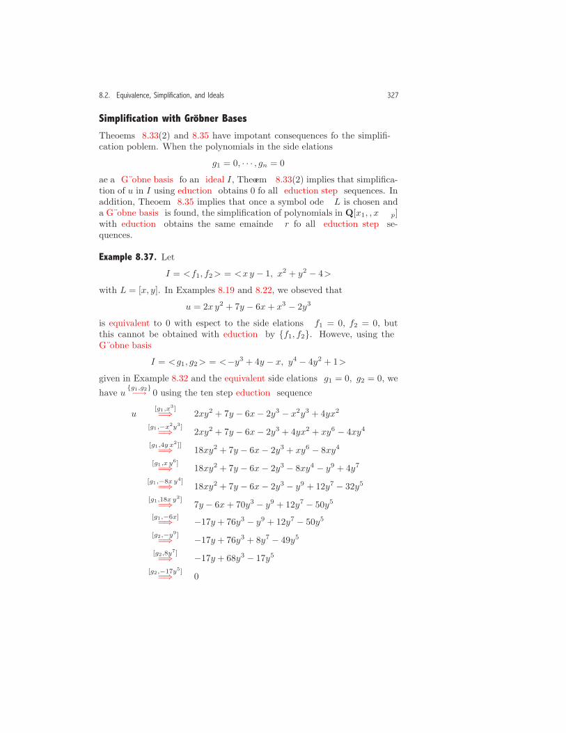
8.2. Equivalence, Simplification, and Ideals 327
Simplification with Grobner Bases
Theorems 8.33(2) and 8.35 have important consequences for the simplifi-cation problem. When the polynomials in the side relations
g1 = 0, · · · , gn = 0
are a Grobner basis for an ideal I, Theorem 8.33(2) implies that simplifica-tion of u in I using reduction obtains 0 for all reduction step sequences. Inaddition, Theorem 8.35 implies that once a symbol order L is chosen anda Grobner basis is found, the simplification of polynomials in Q[x1, . . . , xp]with reduction obtains the same remainder r for all reduction step se-quences.
Example 8.37. Let
I = <f1, f2> = <xy − 1, x2 + y2 − 4>
with L = [x, y]. In Examples 8.19 and 8.22, we observed that
u = 2x y2 + 7y − 6x+ x3 − 2y3
is equivalent to 0 with respect to the side relations f1 = 0, f2 = 0, butthis cannot be obtained with reduction by {f1, f2}. However, using theGrobner basis
I = <g1, g2> = <−y3 + 4y − x, y4 − 4y2 + 1>
given in Example 8.32 and the equivalent side relations g1 = 0, g2 = 0, we
have u{g1,g2}−→ 0 using the ten step reduction sequence
u[g1,x
3]=⇒ 2xy2 + 7y − 6x− 2y3 − x2y3 + 4yx2
[g1,−x2y3]=⇒ 2xy2 + 7y − 6x− 2y3 + 4yx2 + xy6 − 4xy4
[g1,4y x2]]
=⇒ 18xy2 + 7y − 6x− 2y3 + xy6 − 8xy4
[g1,x y6]
=⇒ 18xy2 + 7y − 6x− 2y3 − 8xy4 − y9 + 4y7
[g1,−8x y4]=⇒ 18xy2 + 7y − 6x− 2y3 − y9 + 12y7 − 32y5
[g1,18x y2]
=⇒ 7y − 6x+ 70y3 − y9 + 12y7 − 50y5
[g1,−6x]=⇒ −17y+ 76y3 − y9 + 12y7 − 50y5
[g2,−y9]=⇒ −17y+ 76y3 + 8y7 − 49y5
[g2,8y7]
=⇒ −17y+ 68y3 − 17y5
[g2,−17y5]=⇒ 0.

328 8. Polynomial Simplification with Side Relations
Since a Grobner basis introduces many more opportunities for reductionsteps, it usually produces longer reduction sequences and increases dramat-ically the number of possible sequences. �
A Computational Test for a Grobner Basis
In the remainder of this section we develop a computational test for aGrobner basis. We begin with some new terminology.
Definition 8.38. Let u and v be non-zero monomials, and let L be a listthat defines the variable order. The least common multiple of u and vis a monomial d that satisfies the following three properties.
1. u|d and v|d.2. If u|e and v|e, then d|e.3. The coefficient part of d is 1.
The operator lcm(u, v, L) represents the least common multiple, andwhen L is understood from context, we use the simpler notation lcm(u, v).
The variable part of the monomial
u v
gcd(u, v)
satisfies the three properties of the definition (Exercise 10(a)). An operatorthat obtains the least common multiple is described in Exercise 10a(b).
Definition 8.39. Let u and v be non-zero polynomials, and let L be a listof symbols that defines the variable order. The S-polynomial of u and vis defined by
S(u, v, L) =d
lm(u, L)u− d
lm(v, L)v, (8.71)
whered = lcm(lm(u, L), lm(v, L)).
When L is evident from context, we use the simpler notation S(u, v).
In this definition, d/lm(u, L) and d/lm(v, L) are monomials, and byTheorem 6.25(1),
lm(
d
lm(u, L)u
)= d = lm
(d
lm(v, L)v
).

8.2. Equivalence, Simplification, and Ideals 329
Therefore, in Equation (8.71), the leading monomials ofd u
lm(u, L)and
d v
lm(v, L)cancel.
Example 8.40. Let u = x y − 1 and v = x2 + y2 − 4, and let L = [x, y]define the variable order. Then, d = lcm(x2, x y) = x2y, and
S(u, v, L) =x2 y
x yu− x2 y
x2v = xu− y v = −x− y3 + 4 y.
This polynomial is the one used in Example 8.32 to show that a basis wasnot a Grobner basis. �
A procedure that obtains an S-polynomial is described in Exercise 10a.
Theorem 8.41. The S-polynomials satisfy the following properties.
1. S(u, u) = 0.
2. S(u, v) = −S(v, u).3. If u and v are in an ideal I, then S(u, v) is also in I.
4. If m and n are monomials, then,
S(mu, n v) =A
BS(u, v),
where
A = lcm(lm(mu), lm(n v)), B = lcm(lm(u), lm(v)).
5. Suppose that u and v are non-zero polynomials, and
lm(u) = lm(v) = M.
Then:
(a) lm(S(u, v))≺M .
(b) Iff = c u+ d v
where c and d are rational numbers and lm(f)≺M , then
f = k S(u, v)
where k is a rational number.

330 8. Polynomial Simplification with Side Relations
Proof: The proofs of Parts (1), (2), (3), and (4), which follow from thedefinition, are left to the reader (Exercise 5).
To show (5a), observe in this case S(u, v) = u− v. Since M is elimi-nated from S(u, v), we have lm(S(u, v))≺M .
To show (5b), let V be the variable part of M . We have
u = a V + r, v = b V + s,
where r and s represent lower order monomials, and a and b are non-zerorational numbers. Since f = (c a+d b)V + c r+d s and lm(f)≺M , we havec a+ d b = 0, and
f = c a (u/a) + d b (v/b)
= c a
(V
aVu− V
b Vv
)+
v
b(c a+ d b)
= c a S(u, v). �
The next theorem uses S-polynomials to give a computational test thatdetermines if a basis is a Grobner basis.
Theorem 8.42. Let I = < g1, . . . , gn > where n ≥ 2, and let L be a listof symbols that defines the variable order. The following conditions areequivalent.
1. G = {g1, . . . , gn} is a Grobner basis for I.
2. For all i < j, S(gi, gj)G−→ 0 for all reduction step sequences.
3. For all i < j, S(gi, gj)G−→ 0 for at least one reduction step sequence.
Notice that condition (2) refers to all reduction step sequences, whilecondition (3) refers to at least one reduction step sequence. By statingthe theorem in this way, we can use condition (2) to show that G is not aGrobner basis by finding just one reduction step sequence which does notobtain 0 and can use the weaker condition (3) to show that G is a Grobnerbasis.
Proof of Theorem 8.42: To show that (1) implies (2), if G is a Grobnerbasis, then, since S(gi, gj) is in I, Theorem 8.33(2) implies that
S(gi, gj)G−→ 0.
It is obvious that (2) implies (3).

8.2. Equivalence, Simplification, and Ideals 331
We show that (3) implies (1) using the condition in Theorem 8.33(3).Since the proof for this case is quite involved, we illustrate the basic ideafor a basis with two polynomials {g1, g2}. We will show that the conditionin (3) implies that each f in I = < g1, g2 > has a representation
f = c1g1 + c2g2 (8.72)
such thatlm(f)≡max({lm(c1g1), lm(c2g2)}). (8.73)
Suppose that Equation (8.73) does not hold for a representation where
lm(f)≺M = max({lm(c1g1), lm(c2g2)}). (8.74)
In Example 8.34, we showed that, in this situation, we can find anotherrepresentation for f where Equation (8.73) holds using multiple divisionby a Grobner basis. We take a similar approach here although we can’tsimply divide f by [g1, g2], because the point of the proof is to show that{g1, g2} is a Grobner basis. Instead, we apply the reduction process to arelated polynomial to find a new representation f = d1 g1 + d2 g2 where
M2 = max({lm(d1 g1), lm(d2 g2)})≺M.
If lm(f)≡M2, the proof is complete. If lm(f)≺M2, we repeat the process (afinite number of times) until we find a representation that satisfies Equation(8.73).
The inequality (8.74) implies that in Equation (8.72) the leading mono-mials of c1g1 and c2g2 must cancel, and, therefore,
M = lm(c1g1) = lm(c2g2). (8.75)
Let Vi be the variable part of lm(ci), i = 1, 2. We have
c1 = k1V1 + l1, c2 = k2V2 + l2 (8.76)
where k1 and k2 are rational numbers and l1 and l2 represent the lowerorder monomials with respect to ≺. Define
g = k1V1g1 + k2V2g2. (8.77)
Observe thatf = g + l1g1 + l2g2, (8.78)
and since
lm(V1g1)≡lm(c1g1) = M = lm(c2g2)≡lm(V2g2), (8.79)

332 8. Polynomial Simplification with Side Relations
lm(l1g1)≺M, lm(l2g2)≺M, (8.80)
it follows that g contains the part of f that creates the inequality (8.74).In addition, Theorem 8.41(5b) (applied to V1g1, V2g2, and g), Theorem8.41(4), and Equation (8.79) imply that
g = k S(V1g1, V2g2) = kVMd
S(g1, g2), (8.81)
where k is a rational number,
VM = lcm(lm(V1g1), lm(V2, g2))
is the variable part of M , and
d = lcm(lm(g1), lm(g2)).
Equation (8.81), condition (3), and Theorem 8.17 imply that
gG−→ 0
for some reduction step sequence. Therefore, Theorem 8.18 implies thatthere is a representation
g = e1g1 + e2g2 (8.82)
wherelm(g)≡max({lm(e1)lm(g1), lm(e2)lm(g2)}). (8.83)
In addition,
S(V1g1, V2g2) =VM
lm(V1g1)V1g1 − VM
lm(V2g2)V2g2. (8.84)
Equation (8.79) implies that VM/lm(V1g1) and VM/lm(V2g2) are rationalnumbers, and since the leading monomials in
VMlm(V1g1)
V1g1
andVM
lm(V2g2)V2g2
cancel, it follows from Equations (8.79) and (8.84) that
lm(g)≡lm(S(V1g1, V2g2))≺max({lm(V1g1), lm (V2g2)})≡M. (8.85)

8.2. Equivalence, Simplification, and Ideals 333
Finally, from Equations (8.78) and (8.82), we have the new representation
f = (e1 + l1)g1 + (e2 + l2)g2, (8.86)
where from the relations (8.80), (8.83), and (8.85),
M2 = max({lm((e1 + l1)g1), lm((e2 + l2)g2)})� max({lm(e1g1), lm(l1g1), lm(e2g2), lm(l2g2)})≡ max({lm(g), lm(l1g1), lm(l2g2), })≺ M.
To summarize, we have constructed a new representation for f in Equa-tion (8.86) where lm(f) �M2≺M. If lm(f)≡M2, Theorem 8.33(3) impliesthat {g1, g2} is a Grobner basis. If lm(f)≺M2, we reapply the constructiona finite number of times until a representation is found such that
f = p1 f1 + p2 f2, lm(f)≡max({lm(p1 f1), lm(p2 f2)}).
Therefore, Theorem 8.33(3) implies that {g1, g2} is a Grobner basis. �
Exercises1. Use a CAS to find a Grobner basis for some of the ideals in this section.Note: In Maple use gbasis, in Mathematica use GroebnerBasis, and inMuPAD use groebner::gbasis. Since computer algebra systems use anumber of ordering schemes for monomials, make sure the system uses thelexicographical order. (Implementation: Maple (mws), Mathematica (nb),MuPAD (mnb).)
2. Prove Theorem 8.27.
3. Let I be an ideal in Q[x].
(a) If I = < f1, f2 >, show that I = < gcd(f1, f2) > . Hint: Use theextended Euclidean algorithm.
(b) If I = < f1, . . . , fn >, show that I = < gcd(f1, . . . , fn) > .
4. Let I = < x, y >.
(a) Show that < 3x + 2y, 2x + 3y > is also a basis for I .
(b) Show that I is not a principal ideal. Hint: Suppose that
I = < f(x, y) >,
and use a degree argument to show that if x and y are multiples off(x, y), then f(x, y) is a rational number.

334 8. Polynomial Simplification with Side Relations
5. Suppose that I = < f >. Show that {f} is a Grobner basis for the ideal.
6. Suppose that I = < f1, . . . , fn > where
Variables(fi) ∩Variables(fj) = ∅for i �= j. Show that {f1, . . . , fn} is a Grobner basis for I .
7. Suppose that I = < f1, . . . , fn > where each fi is a monomial. Show that{f1, . . . , fn} is a Grobner basis for I .
8. Consider the ideal I = < f1, f2 >= < y x2 + 1, y3 + 2y − 1 >.
(a) Show that {f1, f2} is not a Grobner basis for I .
(b) Show that {g1, g2} = {x2 + y2 + 2, y3 + 2y− 1} is a Grobner basis forI using Definition 8.30.
9. Prove Theorem 8.35.
10. (a) Let u and v be non-zero monomials. Show that the polynomial
u v
gcd(u, v)
satisfies properties (1) and (2) of Definition 8.38. Hint: See Exercise18, page 35.
(b) Let L be a list of symbols that defines the variable order, and letu and v be non-zero monomials in the symbols in L with rationalnumber coefficients. Give a procedure
Monomial lcm(u, v, L)
that obtains the lcm(u, v, L). If u = 0 or v = 0, return the globalsymbol Undefined.
(c) Let u and v be polynomials, and let L be a list that defines the variableorder. Give a procedure S poly(u, v, L) that returns S(u, v, L) inexpanded form.
11. Prove Theorem 8.41, Parts (1), (2), (3), and (4).
8.3 A Simplification Algorithm
Let u be a polynomial in Q[x1, . . . , xp], and consider the simplification ofu with respect to the side relations f1 = 0, . . . , fn = 0. Our discussionin the previous two sections suggests that our simplification algorithm hastwo steps.
1. Let I = < f1, . . . , fn >, and let L be a list that determines thevariable order. Find a Grobner basis G = {g1, . . . , gm} so thatI = <g1, . . . , gm>.

8.3. A Simplification Algorithm 335
2. Find the simplified form of u as the (reduced) remainder r of thereduction u
G−→ r.
The next theorem shows that this algorithm obtains the two goals ofour simplification algorithm (page 321).
Theorem 8.43. Suppose that F = {f1, . . . , fn}, and let I be the ideal that isgenerated by F . In addition, suppose that G = {g1, . . . , gm} is a Grobnerbasis for I.
1. For u in I, u G−→ 0.
2. If u G−→ r, then uF= r.
3. If u G−→ r, then r is reduced with respect to F .
Proof: Statement (1) is a restatement of Theorem 8.33(2) (page 325).To show (2), Theorem 8.25 states that u G−→ r implies u G= r. Since
I = <f1, . . . , fn> = <g1, . . . , gm>,
the two systems f1 = 0, . . . , fn = 0 and g1 = 0, . . . , gm = 0 have the samesolutions, and therefore u F= r.
The proof of (3), which follows from the definition, is left to the reader(Exercise 1). �
Grobner Basis Algorithm
The first step in a simplification algorithm involves finding a Grobner basisfor an ideal. An algorithm that does this is based on the reduction propertyfor S-polynomials given in Theorem 8.42 on page 330. We illustrate thegeneral approach in the next example.
Example 8.44. Consider the ideal
I = <f1, f2> = <xy + x+ 1, x y2 + y + x2 + 1>,
and let L = [x, y]. Our strategy is to add the non-zero reductions ofS-polynomials to the basis until the third condition in Theorem 8.42 issatisfied. In this example, all reductions are done with the selection schemegiven in Figure 8.1 on page 316.
First, S(f1, f2) = x2 + x− x y3 − y2 − y, and since
S(f1, f2){f1,f2}−→ r = x− 2 y − 1,

336 8. Polynomial Simplification with Side Relations
the condition in Theorem 8.42(2) is not satisfied for this S-polynomial.When this happens, however, since r is in I, we can include it in the basis.Therefore, if f3 = r, we have I = <f1, f2, f3>, and by Theorem 8.15,
S(f1, f2){f1,f2,f3}−→ 0. (8.87)
To determine if {f1, f2, f3} is a Grobner basis, we must also check thatthe reduction condition for S-polynomials is satisfied for S(f1, f3) andS(f2, f3). However,
S(f1, f3) = x+ 2 y2 + y + 1{f1,f2,f3}−→ r = 2 y2 + 3 y + 2, (8.88)
and since r �= 0, we append f4 = r to the basis giving I = <f1, f2, f3, f4>.As before, by Theorem 8.15,
S(f1, f3){f1,f2,f3,f4}−→ = 0.
In addition, a calculation shows that
S(f2, f3) = x y2 + 2 x y + x+ y + 1{f1,f2,f3,f4}−→ = 0.
At this point, since we are using the selection scheme in Figure 8.1, we havethe reduction conditions
S(fi, fj){f1,f2,f3,f4}−→ = 0, i < j = 1, 2, 3.
In fact, some calculation also shows that
S(fi, f4){f1,f2,f3,f4}−→ = 0, i = 1, 2, 3,
and therefore
{f1, f2, f3, f4} = {x y+x+1, x y2+ y+x2+1, x−2 y−1, 2 y2+3 y+2}
is a Grobner basis for I. �
The algorithm we have followed in the last example is known as Buch-berger’s algorithm. We show in Theorem 8.52 below that the algorithmterminates and obtains a Grobner basis for an ideal.
A procedure for Buchberger’s algorithm is given in Figure 8.2. Theinput list F of polynomials generates an ideal, and the input list L ofsymbols determines the variable order. At line 1, the variable G, whicheventually contains the Grobner basis, is initialized to F . The variable P ,

8.3. A Simplification Algorithm 337
Procedure G basis(F,L);Input
F : a list of non-zero polynomials in L;L : a list of symbols;
Outputa list with a Grobner basis;
Local VariablesG,P, i, j, t, s, r;
Begin1 G := F ;2 P := [ ];3 for i := 1 to Number of operands(G) do4 for j := i + 1 to Number of operands(G) do5 P := Join(P, [[Operand(G, i),Operand(G, j)]]);6 while P �= [ ] do7 t := Operand(P, 1);8 P := Rest(P );9 s := S poly(Operand(t, 1),Operand(t, 2), L);10 r := Operand(Reduction(s,G,L), 2);11 if r �= 0 then12 for i from 1 to Number of operands(G) do13 P := Join(P, [[Operand(G, i), r]]);14 G := Join(G, [r]);15 Return(G)
End
Figure 8.2. An MPL procedure for Buchberger’s algorithm. (Implementation:Maple (txt), Mathematica (txt), MuPAD (txt).)
which is a list of two element lists of polynomials from G, is constructed inlines 2–5. This list, which is used to construct the S-polynomials, changesas the algorithm progresses (lines 8, 12–13). For each pass through thewhile loop, we first choose (and remove) a pair t from P , construct anS-polynomial from t (lines 7–9), and then perform the reduction s
G−→ r(line 10). (The S poly procedure is described in Exercise 10, page 334.)We then check the condition in Theorem 8.42 (line 11). If the reducedpolynomial r �= 0, new pairs of polynomials, which are constructed frommembers of the current basis G with r, are added to P , and r is addedto G (lines 12–14). The algorithm terminates when P = [ ], which meansthere are no more S-polynomials to test.

338 8. Polynomial Simplification with Side Relations
In its current form, the G basis procedure returns a basis with someredundant polynomials. The next theorem provides a way to eliminatethis redundancy
Theorem 8.45. Let I = < g1, . . . , gn > where G = {g1, . . . , gn} is aGrobner basis for I, and suppose that L is a list of symbols that definesthe variable order. If
gi{g1,...,gi−1,gi+1,...,gn}−→ 0,
then {g1, . . . , gi−1, gi+1, . . . , gn} is also a Grobner basis for I.
The proof, which follows from the definition of a Grobner basis, is leftto the reader (Exercise 4). �
Example 8.46. In Example 8.44 we considered the ideal
I = <f1, f2> = <xy + x+ 1, x y2 + y + x2 + 1>
where L = [x, y] and showed that
{f1, f2, f3, f4} = {x y+ x+1, x y2 + y+ x2 +1, x− 2y− 1, 2y2 + 3y+ 2}is a Grobner basis for the ideal. However, using the selection scheme in
Figure 8.1, we have f1{f2,f3,f4}−→ 0 and f2
{f3,f4}−→ 0. Therefore,
{f3, f4} = {x− 2y − 1, 2y2 + 3y + 2}is also a Grobner basis for I. �
In Exercise 5 we describe a procedure, based on Theorem 8.45, thateliminates redundant polynomials from a Grobner basis.
In most cases, finding a Grobner basis involves significant computa-tion and coefficient explosion, particularly if the coefficients or degreesare large, or there are many variables, or the algorithm encounters manyS-polynomials that do not reduce to 0. This point is illustrated in the nextexample.
Example 8.47. Consider the ideal
I = <f1, f2> = <2x3y + 3x2 + 6, 5x2 + x+ 3y2 + y + 1>
where L = [x, y]. The G basis procedure forms a basis of eight polynomials:

8.3. A Simplification Algorithm 339
f1 = 2 x3y + 3 x2 + 6,f2 = 5 x2 + x+ 3 y2 + y + 1,
f3 = −35xy3 − 1
5xy2 − 4
25xy − 3
10x+
325
y3 − 4350
y2 − 1350
y +2710
,
f4 =310
xy2 +73750
xy − 2225
x− 325
y5 − 225
y4 − 38375
y3 +23750
y2
+1250
y − 1950
,
f5 = − 355111250
xy − 4297750
x− 625
y7 − 625
y6 − 128125
y5
− 4481125
y4 − 1621311250
y3 − 61885625
y2 +134325625
y − 389250
,
f6 = −55134547958770
x− 647416266325
y7 − 540886266325
y6 − 8071024798975
y5
−265583087190775
y4 − 357057262396925
y3 − 1864529191754
y2 +37229059914381550
y
−970717974793850
,
f7 =16203551
y9 +21603551
y8 +27003551
y7 +10503551
y6 +9553
y5 +137853551
y4
−292953551
y3 − 207853551
y2 +527853551
y +186753551
,
f8 =9003551
y8 +9003551
y7 +12003551
y6 +55010653
y5 +34753551
y4 +65003551
y3
−5532510653
y2 − 54003551
y +311253551
.
After removing redundant polynomials from the basis, we obtain a Grobnerbasis {f6, f8}. �
Both the Grobner basis and the path taken by the algorithm are de-pendent on the choice of reduction selection scheme, the order of the siderelations, and the symbol order. This point is illustrated in the next ex-ample.
Example 8.48. Let
F = {f1, f2, f3} = {x y + x+ z − 3, x z + y + x2 + 1, y + z2 + x+ 2},L = [x, y, z], and let I be the ideal generated by F . For the basis or-der [f1, f2, f3], the G basis procedure obtains a Grobner basis with sevenmembers, and, once redundant polynomials are eliminated, we have theGrobner basis

340 8. Polynomial Simplification with Side Relations
{y + z2 + x+ 2,
− 2 y + 5 z + z4 − 2 z2 − 10,− 5 z3 + 13 z2 − z6 − 2 z4 + z5 − 18 z + 20
}.
On the other hand, for the basis order [f2, f3, f1], the G basis procedure ob-tains a Grobner basis with nine members, and once redundant polynomialsare eliminated, we have the Grobner basis{
y + z2 + x+ 2,
3 z + 6 y − 7 z2 − z4 + 5 z3 + z6 − z5 + 10,5/3 z3 − 13/3 z2 + 1/3 z6 + 2/3 z4 − 1/3 z5 + 6 z − 20/3
}. �
Termination of Buchberger’s Algorithm
In order to show that Buchberger’s algorithm terminates, we must look atsome more advanced concepts from the theory of ideals. First, in mosttextbooks on this subject, an ideal is defined in a more general way thanwe have given in Definition 8.26 (page 321).
Definition 8.49. A set I ⊂ Q[x1, . . . , xp] is an ideal if it satisfies thefollowing two conditions.
1. If u and v are in I, then u+ v is also in I.
2. If u is in I and c is in Q[x1, . . . , xp], then c u is also in I.
In this definition an ideal is defined as any set of polynomials thatsatisfies properties (1) and (2) of Theorem 8.27 on page 322. Although thisdefinition appears more general than the one in Definition 8.26, the twodefinitions are actually equivalent as long as we restrict our attention tothe domainQ[x1, . . . , xp]. This fact is the content of the following theorem,known as the Hilbert Basis Theorem.
Theorem 8.50. Let I be an ideal in the sense of Definition 8.49 whichis contained in Q[x1, . . . , xp]. Then, I is generated by a finite basis ofpolynomials.
The proof of the theorem is given in the references cited at the end ofthe chapter. �
The ideal described in the next definition is used in the proof of thetermination of Buchberger’s algorithm.

8.3. A Simplification Algorithm 341
Definition 8.51. Let F = {f1, . . . , fn} be a set of non-zero polynomials thatgenerate an ideal I, and let L be a list of symbols. The leading monomialideal of F is the ideal
LMI(F ) = < lm(f1), . . . , lm(fn)> .
Theorem 8.52. Let F = [f1, . . . , fn] be a list of non-zero polynomials thatgenerate an ideal I, and let L be a list of symbols that determines the vari-able order. Then, the G basis procedure terminates and returns a Grobnerbasis for I.
Proof: The proof of termination, which is based on the Hilbert BasisTheorem, is by contradiction. If the algorithm does not terminate, there isan infinite sequence of sets
G1 = {f1, . . . , fn},G2 = G1 ∪ {r1},
...Gk+1 = Gk ∪ {rk},
...
where rk �= 0 is the reduction with respect to Gk of the S-polynomial oftwo polynomials in Gk. Although
G1 ⊂ G2 ⊂ · · ·Gk ⊂ Gk+1 ⊂ · · · , (8.89)
we still haveGk ⊂ I, k = 1, 2, . . . . (8.90)
In order to apply the Hilbert Basis Theorem, we need to introduceanother ideal into the discussion. From (8.89), we have
LMI(G1) ⊂ LMI(G2) ⊂ · · · ⊂ LMI(Gk) ⊂ LMI(Gk+1) ⊂ · · · . (8.91)
In addition, since rk is reduced with respect to Gk, lm(rk) is not divisibleby the leading monomial of any polynomial in Gk, and therefore
LMI(Gk) �= LMI(Gk+1). (8.92)
DefineJ = ∪∞k=1LMI(Gk),

342 8. Polynomial Simplification with Side Relations
where the notation indicates that J is the union of all the ideals LMI(Gk),k = 1, 2, . . .. Observe that J is also an ideal (in the sense of Definition 8.49),which is included in Q[x1, . . . , xp]. Therefore, the Hilbert Basis Theoremimplies that it has a finite basis
J = <p1, . . . , pm>, (8.93)
where each polynomial pj is in some LMI(Gkj ) (which depends on j). Sincethe basis in Equation (8.93) is finite, there is a positive integer k′ where
{p1, . . . , pm} ⊂ LMI(Gk′ ),
and therefore
LMI(Gk) = LMI(Gk′ ), for k ≥ k′. (8.94)
However, since (8.92) and (8.94) cannot both be true, we reach a contra-diction which implies that the G basis algorithm terminates.
To complete the proof, we must show that the set Gk′ is a Grobnerbasis for I. First, since F ⊂ Gk′ , Equation (8.90) implies that Gk′ is a
basis for I. In addition, by Equation (8.94), for f , g in Gk′ , S(f, g)Gk′−→ 0,
and therefore Theorem 8.42 implies that Gk′ is a Grobner basis for I. �
Simplification
Before we present our simplification procedure, we need to address theproblem of side relation consistency. The following theorem shows thatthis question is easily addressed as part of the simplification process.
Theorem 8.53. Let F = {f1, . . . , fn} be a set of non-zero polynomials, andlet I be the ideal generated by F . Then, the system f1 = 0, . . . , fn = 0is inconsistent if and only if each Grobner basis for I contains a non-zeroconstant polynomial.
Proof: The original system of side relations and the system of side relationsdetermined by a Grobner basis have the same solutions. Therefore, if theGrobner basis contains a non-zero constant c, we have a side relation c = 0which implies that the system is inconsistent.
The proof of the implication in the reverse direction, which is moreinvolved, is given in the references cited at the end of the chapter. �
Example 8.54. In Example 8.23 we showed that the system of equations
f1 = x y + x+ 2y + 3 = 0, f2 = x y + 2y + 1 = 0
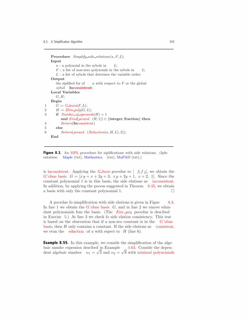
8.3. A Simplification Algorithm 343
Procedure Simplify side relations(u, F, L);Input
u : a polynomial in the symbols in L;F : a list of non-zero polynomials in the symbols in L;L : a list of symbols that determines the variable order;
Outputthe simplified form of u with respect to F or the globalsymbol Inconsistent;
Local VariablesG,H ;
Begin1 G := G basis(F,L);2 H := Elim poly(G,L);3 if Number of operands(H) = 1
and Kind(Operand(H, 1)) ∈ {integer, fraction} then4 Return(Inconsistent)5 else6 Return(Operand(Reduction(u,H,L), 2));
End
Figure 8.3. An MPL procedure for simplifications with side relations. (Imple-mentation: Maple (txt), Mathematica (txt), MuPAD (txt).)
is inconsistent. Applying the G basis procedure to [f1.f2], we obtain theGrobner basis G = [x y + x + 2y + 3, x y + 2y + 1, x + 2, 1]. Since theconstant polynomial 1 is in this basis, the side relations are inconsistent.In addition, by applying the process suggested in Theorem 8.45, we obtaina basis with only the constant polynomial 1. �
A procedure for simplification with side relations is given in Figure 8.3.In line 1 we obtain the Grobner basis G, and in line 2 we remove redun-dant polynomials from the basis. (The Elim poly procedure is describedin Exercise 5.) At line 3 we check for side relation consistency. This testis based on the observation that if a non-zero constant is in the Grobnerbasis, then H only contains a constant. If the side relations are consistent,we return the reduction of u with respect to H (line 6).
Example 8.55. In this example, we consider the simplification of the alge-braic number expression described in Example 4.63. Consider the depen-dent algebraic numbers α1 =
√2 and α2 =
√8 with minimal polynomials
344 8. Polynomial Simplification with Side Relations
p1(x1) = x21 − 2, p2(x2) = x2
2 − 8, and dependence relation
h(x1, x2) = 2 x1 − x2 = 0, (8.95)
and consider the expression
u = α21 + 2 a2
2 + a21 a
22 − 8 a1 a2 − 2
which simplifies to 0. Simplification of u with division by the minimalpolynomials p1(α1) and p2(α2) obtains
u = −8α1 α2 + 32
rather than the simplified form u = 0. However,
Simplify side relations(u, [p1(α1), h(α1, α2)], [α1, α2])→ 0
and
Simplify side relations(u, [p2(α1), h(α1, α2)], [α1, α2])→ 0.
Observe that, in both cases, we obtain the simplified form using only oneof the minimal polynomials together with the dependence relation. �
Appraisal of the Simplification Algorithm
Practical Limitations. Although the simplification algorithm achieves thegoals listed on page 321, it is most useful as a test for zero equivalenceat least for expressions that have a representation in the form (8.64). How-ever, when an input expression does not simplify to 0, the algorithm canreturn a surprisingly complex expression. This point is illustrated in thenext example.
Example 8.56. Let
I = <f1, f2> = <2x3y + 3x2 + 6, 5x2 + x+ 3y2 + y + 1>
with L = [x, y] which was considered in Example 8.47 on page 338, andconsider the simplification of
u = f1 + f2 + x (8.96)= 2x3y + 8x2 + 2x+ 3y2 + y + 7
with respect to the side relations f1 = 0 and f2 = 0. It is apparent fromEquation (8.96) that u simplifies to x with respect to these side relations.

8.3. A Simplification Algorithm 345
In fact, using the Reduction procedure, we obtain u{f1,f2}−→ x. However,
simplifying with reduction by the Grobner basis obtained in Example 8.47,we obtain a much more involved expression
r =372290599827018205
y − 932264555134547
y2 − 71411452275672735
y3 − 372508821205595
y5
− 53116616827018205
y4 − 11653488275672735
y7 − 9735948275672735
y6 − 97071797275672735
.
The problem here is the simple expression x in Equation (8.96) is notreduced with respect to the Grobner basis. However, reduction with theGrobner basis can determine that r − x simplifies to 0. �
Theoretical Limitations. In the next example we show that reduction withGrobner bases cannot always solve the zero equivalence problem.
Example 8.57. Let
F = {f1, f2} = {x2 − 2x+ y2 − 4y + 1, x2 + 4x+ y2 − 4y + 7}
with L = [x, y], and consider the simplification of u = 2x + 3y − 4 withrespect to the side relations f1 = 0, f2 = 0. In this case, the side relationsrepresent two circles that intersect at the single point (x, y) = (−1, 2), andsince u evaluates to 0 at this point, u F=0.
However, in this case we cannot reduce u to 0 even with a Grobnerbasis. Indeed, a Grobner basis for the ideal I = <f1, f2> is
G = {g1, g2} = {−6x− 6, y2 − 4y + 4},
and uG−→ 3y − 6. �
This example shows that the relationship between equivalence and reductionis not as straightforward as we would like. However, a theoretical relation-ship between the two concepts is given in the following theorem.
Theorem 8.58. Let F = {f1, . . . , fn} be a set of non-zero polynomials inQ[x1, . . . , xp], and consider the side relations
f1 = 0, . . . , fn = 0. (8.97)
In addition, let G be a Grobner basis for I =< f1, . . . , fn >. Then, u F= 0if and only if um G−→ 0 for some positive integer m.

346 8. Polynomial Simplification with Side Relations
In other words, u simplifies to 0 within the context of the side relationsin (8.97) if and only if um can be simplified to 0 using reduction with aGrobner basis. The proof of the theorem, which depends on some involvedconcepts from the theory of ideals, is given in the references cited at theend of this chapter. �
Example 8.59. Consider the side relations and polynomial u from Example8.57 above. In this case, u2 G=⇒ 0 using the reduction step sequence
u2 = 4x2 + 12x y − 16x+ 9y2 − 24y + 16[4x2, g1]=⇒ 12x y − 20x+ 9y2 − 24y + 16
[12x y, g1]=⇒ −20x+ 9y2 − 36y + 16
[−20x, g1]=⇒ 9y2 − 36y + 16
[9y2, g2]=⇒ 0. �
Exercises1. Prove Theorem 8.43(3).
2. Use Buchberger’s algorithm to find a Grobner basis for each of the followingideals. In addition, remove any redundant polynomials from the Grobnerbasis. In each case, the variable order is given by L = [x, y].
(a) I = <xy − 1, x2 + y2 − 4>.
(b) I = <x2 y − 1, x + y2 − 4>.
(c) I = <x2 + x y + y2, x y>.
(d) I = <x3 y + x2 − 1, x + y2 + 1>.
(e) I = <x3 y + x2 − 1, x y2 + y + 1>.
(f) I = <x2 − 2, x2 + 2x y + 2, y2 − 2>.
3. Let F = {f1, f2, f3} = {x y − 1, x z − 1, y z − 1}, and let I be the idealgenerated by F .
(a) Find a Grobner basis for I .
(b) Using the simplification algorithm in this section show that
3 x y zF=x + y + z.
4. Prove Theorem 8.45.
5. Let G be a set of polynomials which is a Grobner basis for an ideal, andlet L be a list of symbols that defines the variable order. Give a procedureElim poly(G,L) that eliminates the redundant polynomials from G usingthe condition described in Theorem 8.45.
8.3. A Simplification Algorithm 347
6. Suppose that f1, . . . , fn are non-zero polynomials in Q[x]. Suppose thatwe use the G basis procedure followed by Elim poly procedure (Exercise 5)to find a Grobner basis for I =< f1, . . . , fn >. Explain why this processproduces a basis with one polynomial which is a (non- monic) greatestcommon divisor of f1, . . . , fn. Hint: See Exercise 3, page 333.
7. Consider the polynomial u = x + 3y − 7 and the two side relations
f1 = x y−2x−y+2 = 0, f2 = x4−4x3 +6x2−4x+y3−6y2 +12y−7 = 0.
(a) Show that u{f1,f2}
= 0 with respect to the side relations, but that thiscannot be obtained by reduction with the Grobner basis G for theideal I = <f1, f2>.
(b) Find a positive integer m such that um G−→ 0.
8. Let F = [f1, . . . , fn] be a list of non-zero polynomials that is a basis for anideal I , and let L be a list of variables that defines the variable order. Letu be a polynomial in I . Give a procedure
Represent basis(u, F, L)
that finds a representation for u in terms of the basis F . Notice thatthis can only be done directly with reduction when F is a Grobner basis.Therefore, if F is not a Grobner basis, you will need to modify the G basisprocedure so that it keeps track of a representation of each member of theGrobner basis in terms of F , and then uses this information along with therepresentation of u in terms of a Grobner basis to find the representationof u in terms of F .
9. Consider the ideal
I = <f1, f2> = <xy −√
2, x2 + y2 − 4√
2 >
which is included in the domain Q√
2 [x, y]. Find a Grobner basis for I .
Hint: α =√
2 satisfies α2 − 2 = 0.
10. Grobner basis computation can be used to compute (non- monic) greatestcommon divisors of polynomials with one variable (Exercise 3, page 333).How can you use a Grobner basis computation to compute the gcd ofu = x2 − 2 and v = x2 − 2
√2x + 2 in Q
√2 [x]?
11. Consider the algebraic number u = 1 + 2√
2 + 3√
3. How can you use thesimplification algorithm in this section to find the multiplicative inverse ofu in the field Q(
√2,√
3)?
Further Reading
In this chapter we have given an introduction to the concept of a Grobner basis.
There is, however, much more to this subject. A good starting point for this

348 8. Polynomial Simplification with Side Relations
material is Geddes, Czapor, and Labahn [39], Chapter 10. Adams and Loustau-
nau [1] is a comprehensive introduction to both the theory and applications of
Grobner bases. Our approach in Theorem 8.42, is similar to the one given in this
book which contains the complete proof as well as the proofs for Theorems 8.50,
8.53 and 8.58. Becker, Weispfenning, and Kredel [6] gives a more advanced (and
theoretical) discussion of Grobner bases, including an algorithm to compute the
power m in Theorem 8.58. Chou [20] describes how Grobner bases are used for
the mechanical development of proofs in geometry. The article by Buchberger
[18], the inventor of Grobner bases, is of historical interest.
9
Polynomial Factorization
The goal of this chapter is the complete description of a modern algorithmfor the factorization of polynomials in Q[x] in terms of irrreducible poly-nomials.
In Section 9.1 we describe an algorithm that obtains a partial factor-ization of a polynomial. The algorithm can separate factors of differentmultiplicities as in
x5 + 7 x4 + 17 x3 + 17 x2 + 7 x+ 1 = (x+ 1)(x2 + 3 x+ 1
)2,
but is unable to separate factors of the same multiplicity as in
x3 + 4 x2 + 4 x+ 1 = (x+ 1)(x2 + 3 x+ 1
).
This factorization is important, however, because it reduces the factoriza-tion problem to polynomials without multiple factors. In Section 9.2 wedescribe the classical approach to factorization, which is known as Kro-necker’s algorithm. This algorithm is primarily of historical interest be-cause it is much too slow to be used in practice. In Section 9.3 we describean algorithm that factors polynomials in Zp[x]. Although this algorithmis important in its own right, it is included here because it plays a role inthe modern approach for factorization in Q[x]. Finally, in Section 9.4 wedescribe a modern factorization algorithm, known as the Berlekamp-Henselalgorithm, which uses a related factorization in Zp[x] together with a liftingalgorithm to obtain the factorization in Q[x].
The efficient factorization of polynomials is a difficult computationalproblem. For this reason, both the mathematical and computational tech-niques in this chapter are more involved than those in previous chapters.
349

350 9. Polynomial Factorization
9.1 Square-Free Polynomials and Factorization
A square-free polynomial is one without any repeated factors. In this sec-tion we examine the square-free concept and describe an algorithm thatfactors a polynomial that is not square-free in terms of square-free factors.This type of factorization is the easiest one to obtain and is an importantfirst step in the irrreducible factorization of polynomials.
Square-Free Polynomials
The formal definition of a square-free polynomial reflects the origin of theterm “square-free.”
Definition 9.1. Let F be a field. A polynomial u in F[x] is square-freeif there is no polynomial v in F[x] with deg(v, x) > 0 such that v2|u.
Although the definition is expressed in terms of a squared factor, itimplies that the polynomial does not have a factor of the form vn withn ≥ 2.
Example 9.2. The polynomial u = x2+3 x+2 = (x+1) (x+2) is square-free,while u = x4 + 7 x3 + 18 x2 + 20 x+ 8 = (x+ 1) (x+ 2)3 is not. �
The square-free property can also be described in terms of the irrreduciblefactorization of a polynomial.
Theorem 9.3. Suppose that u is a polynomial in F[x] with an irrreduciblefactorization
u = c pn11 pn2
2 · · · pns−1s−1 pns
s .
Then, u is square-free if and only if ni = 1 for 1 ≤ i ≤ s.
The proof, which is straightforward, is left to the reader (Exercise 4). �
Theorem 9.5 (below) describes a simple test that determines if a poly-nomial is square-free. This test involves the derivative of a polynomial qin F[x], which is defined using the ordinary differentiation rules given incalculus. For a monomial q = a xn, the derivative q′ is given by
q′ =
0, if n = 0,(a+ · · ·+ a)︸ ︷︷ ︸
n
xn−1, if n > 0, (9.1)

9.1. Square-Free Polynomials and Factorization 351
where the notation indicates the sum has n copies of a. The derivative ofa polynomial is defined as the sum of the derivatives of its monomials.
In Equation (9.1), we have resisted using the simpler expression q′ =n axn because the integer n may not be in the field F. For example, forq = 2 x4 + x+ 2 in Z3[x],
q′ = (2 + 2 + 2 + 2)x3 + 1 = 2 x3 + 1.
With this derivative definition as a staring point, we can obtain theordinary sum and product rules for differentiation.
In the proof of Theorem 9.5 (below), we use the fact that a polynomialu with positive degree has a derivative which is not the zero polynomial.Unfortunately, for some coefficient fields F, this property is not true. Forexample, in Z3[x], we have
(x3 + 1)′ = (1 + 1 + 1)x2 = 0 · x2 = 0.
However, if F contains the integers Z, the property does hold.1
Theorem 9.4. Let F be a field that contains Z, and suppose that u is apolynomial in F[x] with positive degree. Then, u′ is not the zero polynomial.
Proof: Let u = an xn + · · · + a0, where n > 0 and an �= 0. For the
leading monomial an xn, the derivative is n anxn−1. Since a field has no
zero divisors, the coefficient n an �= 0, and, therefore, the derivative is notthe zero polynomial. �
For the remainder of this section, we assume that all fields contain Z.
Theorem 9.5. Let F be a field that contains Z, and let u be a polynomialin F[x]. Then, u is square-free if and only if gcd(u, u′) = 1.
Proof: We prove the theorem by proving its negation, namely, u is notsquare-free if and only if gcd(u, u′) �= 1.
Let’s suppose first that u is not square-free, which means there arepolynomials v and w, with deg(v) > 0, such that u = v2 w. Differentiatingthis expression, we have
u′ = 2 v v′ w + v2 w′.
1In abstract algebra textbooks, a field F that contains the integers Z is called a fieldof characteristic 0.

352 9. Polynomial Factorization
Since v divides each term of the sum, it also divides u′, and since v also di-vides u, it divides gcd(u, u′) as well. Therefore, deg(gcd(u, u′)) ≥ deg(v) >0 which implies that gcd(u, u′) �= 1.
We show that the implication goes in the other direction as well. Ifgcd(u, u′) �= 1, there is an irrreducible polynomial v with positive degreethat divides both u and u′. Therefore,
u = q1 v, u′ = q2 v, (9.2)
and differentiating the first expression, we have
u′ = q1 v′ + q′1 v.
In this expression, v divides both u′ and q′1 v, which implies that
v|q1 v′.
Since v is irrreducible, it divides one of the terms in this product (Theorem4.29(2), page 133). However, by Theorem 9.4, v′ �= 0, and since deg(v′) <deg(v), we have v /| v′. Therefore, v|q1 and so, q1 = r v. Substitutingthis expression into u, we obtain u = r v2, which implies that u is notsquare-free. �
Example 9.6. Consider the polynomial u = x3+1 in Q[x]. Then, u′ = 3 x2
and gcd(u, u′) = 1 which means that u is square-free. However, u can befactored as u = (x+ 1)(x2 − x+ 1). �
Since the square-free concept is so closely connected to the gcd concept,it is not surprising that the property does not depend on the size of thecoefficient field. This is the content of the next theorem.
Theorem 9.7. Suppose that F1 and F2 are fields with Z contained in F1
and F1 contained in F2. Then, if u is square-free as a polynomial in F1[x],it is also square-free as a polynomial F2[x].
Proof: The proof follows from the observation that for u in F1[x], thecomputation of gcd(u, u′) (using differentiation and Euclid’s algorithm)involves operations in F1, and so its value does not change if u is viewedas a polynomial in F2[x]. �
Example 9.8. Since the polynomial u = x2 − 2 is square-free in Q[x], it isalso square-free in Q(
√2)[x]. On the other hand, x2 − 2 is irrreducible in
Q[x], but can be factored as (x−√2)(x+√2) in Q(√2)[x]. �
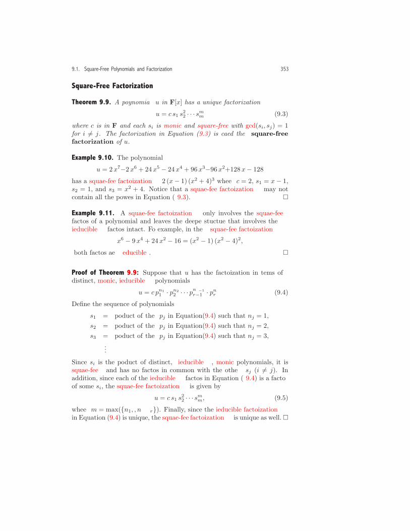
9.1. Square-Free Polynomials and Factorization 353
Square-Free Factorization
Theorem 9.9. A polynomial u in F[x] has a unique factorization
u = c s1 s22 · · · smm (9.3)
where c is in F and each si is monic and square-free with gcd(si, sj) = 1for i �= j. The factorization in Equation (9.3) is called the square-freefactorization of u.
Example 9.10. The polynomial
u = 2 x7−2 x6 + 24 x5 − 24 x4 + 96 x3−96 x2+128 x− 128
has a square-free factorization 2 (x− 1) (x2 + 4)3 where c = 2, s1 = x − 1,s2 = 1, and s3 = x2 + 4. Notice that a square-free factorization may notcontain all the powers in Equation (9.3). �
Example 9.11. A square-free factorization only involves the square-freefactors of a polynomial and leaves the deeper structure that involves theirrreducible factors intact. For example, in the square-free factorization
x6 − 9 x4 + 24 x2 − 16 = (x2 − 1) (x2 − 4)2,
both factors are reducible. �
Proof of Theorem 9.9: Suppose that u has the factorization in terms ofdistinct, monic, irrreducible polynomials
u = c pn11 · pn2
2 · · · pnr−1r−1 · pnr
r . (9.4)
Define the sequence of polynomials
s1 = product of the pj in Equation(9.4) such that nj = 1,s2 = product of the pj in Equation(9.4) such that nj = 2,s3 = product of the pj in Equation(9.4) such that nj = 3,
...
Since si is the product of distinct, irrreducible, monic polynomials, it issquare-free and has no factors in common with the other sj (i �= j). Inaddition, since each of the irrreducible factors in Equation (9.4) is a factorof some si, the square-free factorization is given by
u = c s1 s22 · · · smm, (9.5)
where m = max({n1, . . . , nr}). Finally, since the irrreducible factorizationin Equation (9.4) is unique, the square-free factorization is unique as well. �
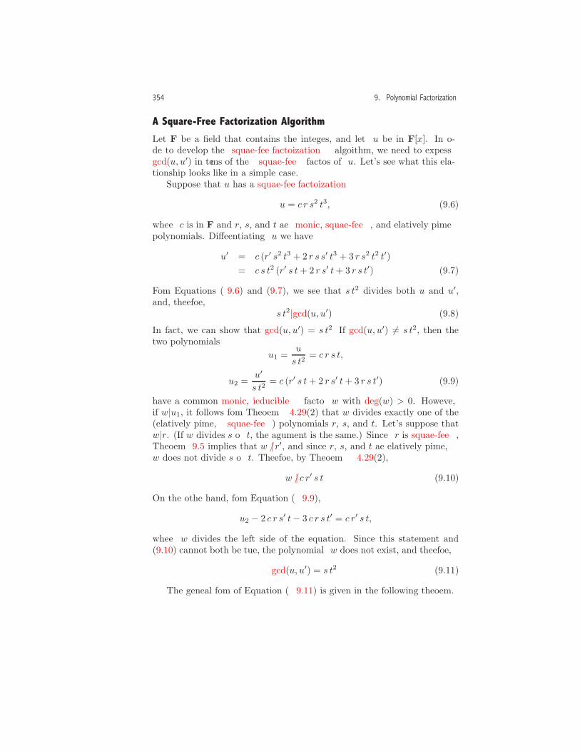
354 9. Polynomial Factorization
A Square-Free Factorization Algorithm
Let F be a field that contains the integers, and let u be in F[x]. In or-der to develop the square-free factorization algorithm, we need to expressgcd(u, u′) in terms of the square-free factors of u. Let’s see what this rela-tionship looks like in a simple case.
Suppose that u has a square-free factorization
u = c r s2 t3, (9.6)
where c is in F and r, s, and t are monic, square-free, and relatively primepolynomials. Differentiating u we have
u′ = c (r′ s2 t3 + 2 r s s′ t3 + 3 r s2 t2 t′)= c s t2 (r′ s t+ 2 r s′ t+ 3 r s t′). (9.7)
From Equations (9.6) and (9.7), we see that s t2 divides both u and u′,and, therefore,
s t2|gcd(u, u′). (9.8)
In fact, we can show that gcd(u, u′) = s t2. If gcd(u, u′) �= s t2, then thetwo polynomials
u1 =u
s t2= c r s t,
u2 =u′
s t2= c (r′ s t+ 2 r s′ t+ 3 r s t′) (9.9)
have a common monic, irrreducible factor w with deg(w) > 0. However,if w|u1, it follows from Theorem 4.29(2) that w divides exactly one of the(relatively prime, square-free) polynomials r, s, and t. Let’s suppose thatw|r. (If w divides s or t, the argument is the same.) Since r is square-free,Theorem 9.5 implies that w /| r′, and since r, s, and t are relatively prime,w does not divide s or t. Therefore, by Theorem 4.29(2),
w /| c r′ s t. (9.10)
On the other hand, from Equation (9.9),
u2 − 2 c r s′ t− 3 c r s t′ = c r′ s t,
where w divides the left side of the equation. Since this statement and(9.10) cannot both be true, the polynomial w does not exist, and therefore,
gcd(u, u′) = s t2. (9.11)
The general form of Equation (9.11) is given in the following theorem.

9.1. Square-Free Polynomials and Factorization 355
Theorem 9.12. Suppose that F is a field that contains Z, and suppose thatu in F[x] has the square-free factorization u = c s1 s
22 · · · smm with m ≥ 2.
Then,
gcd(u, u′) =m∏i=2
si−1i . (9.12)
Proof: The general proof, which follows the lines of the above argument,is left to the reader (Exercise 7). �
To motivate the square-free factorization algorithm, suppose that u isa monic polynomial with a square-free factorization
u = q r2 s3 t4,
where q, r, s, and t are monic, square-free, and relatively prime polynomi-als. We show that it is possible to find the factors q, r, s and t using onlythe polynomial division and greatest common divisor operations.
First, let’s see how to obtain the factor q. Using Theorem 9.12, let
R = gcd(u, u′) = r s2 t3 (9.13)
where the exponent of each factor in R is one less than the correspondingexponent in u. Next, using polynomial division, we obtain a polynomialthat is the product of each polynomial in the factorization:
F = quot(u,R) = q r s t. (9.14)
LetG = gcd(R,F ) = r s t, (9.15)
where all the factors except q appear to the first power. Finally, we obtainq with the division
F
G= quot(q r s t, r s t) = q. (9.16)
To obtain the next factor r, we redefine R by dividing the old value of R(from Equation (9.13)) by the value for G (from Equation (9.15)),
R = quot(r s2 t3, r s t) = s t2, (9.17)
and redefine F as the current value of G in Equation (9.15):
F = r s t. (9.18)

356 9. Polynomial Factorization
Procedure Square free factor(u, x);Input
u : a polynomial in F[x] where all field operationsin F are obtained with automatic simplificationand Z is contained in F;
x : a symbol;Output
The square-free factored form of the polynomial u;Local Variables
U, c, P,R, F, j,G, s;Begin
1 if u = 0 then Return(u)2 else3 c := Leading Coefficient gpe(u, x);4 U := Algebraic expand(u/c);5 P := 1;6 R := Polynomial gcd(U, Derivative(U,x), x);7 F := Quotient(U,R,x);8 j := 1;9 while R �= 1 do10 G := Polynomial gcd(R,F, x);11 s := Quotient(F,G, x);12 P := P ∗ sj ;13 R := Quotient(R,G, x);14 F := G;15 j := j + 1;16 P := P ∗ F j ;17 Return(c ∗ P )
End
Figure 9.1. The MPL square-free factorization procedure. (Implementation:Maple (txt), Mathematica (txt), MuPAD (txt).)
Then, repeating the operations in Equations (9.15) and (9.16), we obtainthe polynomial r:
G = gcd(R,F ) = s t,F
G= quot(r s t, s t) = r.
Continuing in this fashion we find all the components in the factorization.
A procedure that obtains the square-free factorization using these op-erations is given in Figure 9.1. In lines 3 and 4 we remove the leading
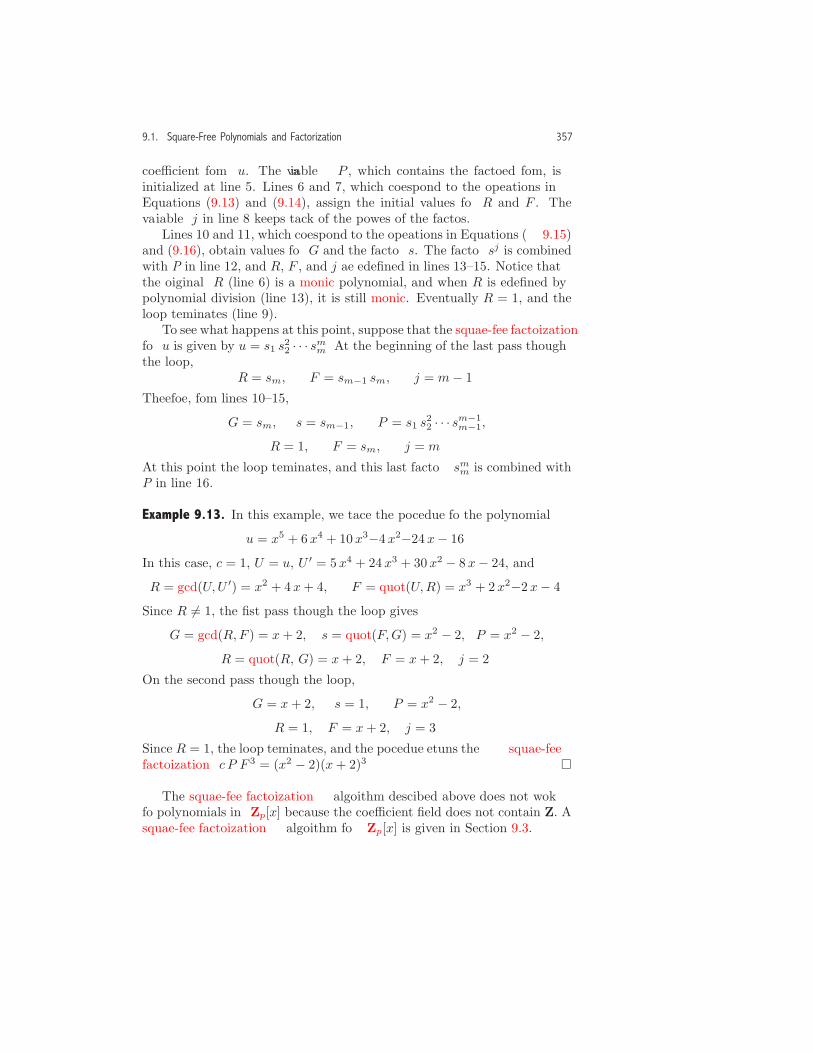
9.1. Square-Free Polynomials and Factorization 357
coefficient from u. The variable P , which contains the factored form, isinitialized at line 5. Lines 6 and 7, which correspond to the operations inEquations (9.13) and (9.14), assign the initial values for R and F . Thevariable j in line 8 keeps track of the powers of the factors.
Lines 10 and 11, which correspond to the operations in Equations (9.15)and (9.16), obtain values for G and the factor s. The factor sj is combinedwith P in line 12, and R, F , and j are redefined in lines 13–15. Notice thatthe original R (line 6) is a monic polynomial, and when R is redefined bypolynomial division (line 13), it is still monic. Eventually R = 1, and theloop terminates (line 9).
To see what happens at this point, suppose that the square-free factorizationfor u is given by u = s1 s
22 · · · smm. At the beginning of the last pass through
the loop,R = sm, F = sm−1 sm, j = m− 1.
Therefore, from lines 10–15,
G = sm, s = sm−1, P = s1 s22 · · · sm−1
m−1,
R = 1, F = sm, j = m.
At this point the loop terminates, and this last factor smm is combined withP in line 16.
Example 9.13. In this example, we trace the procedure for the polynomial
u = x5 + 6 x4 + 10 x3−4 x2−24 x− 16.
In this case, c = 1, U = u, U ′ = 5 x4 + 24 x3 + 30 x2 − 8 x− 24, and
R = gcd(U,U ′) = x2 + 4 x+ 4, F = quot(U,R) = x3 + 2 x2−2 x− 4.
Since R �= 1, the first pass through the loop gives
G = gcd(R,F ) = x+ 2, s = quot(F,G) = x2 − 2, P = x2 − 2,
R = quot(R, G) = x+ 2, F = x+ 2, j = 2.
On the second pass through the loop,
G = x+ 2, s = 1, P = x2 − 2,
R = 1, F = x+ 2, j = 3.
Since R = 1, the loop terminates, and the procedure returns the square-freefactorization c P F 3 = (x2 − 2)(x+ 2)3. �
The square-free factorization algorithm described above does not workfor polynomials in Zp[x] because the coefficient field does not contain Z. Asquare-free factorization algorithm for Zp[x] is given in Section 9.3.

358 9. Polynomial Factorization
Square-Free Factorization in Z[x]Let’s consider briefly the square-free factorization of polynomials in Z[x]using the gcd operations described in Section 6.3. In this case, both thetheorems and algorithm are similar to those given above with modificationsto account for the form of the gcd in this setting.
Since a polynomial in Z[x] with positive degree has a non-zero deriva-tive, a theorem similar to Theorem 9.5 is valid. However, since the gcdin Z[x] is unit normal rather than monic, the theorem takes the followingform.
Theorem 9.14. Let u be a polynomial in Z[x]. Then, u is square-free ifand only if deg(gcd(u, u′)) = 0.
In this setting, u has a unique square-free factorization of the form
u = c s1 s22 · · · smm, (9.19)
where2
c = sign(lc(u)) cont(u), (9.20)and the si are square-free, primitive, unit normal, and relatively prime(Exercise 12). In this setting, the analogue of Equation (9.12) is
gcd(u, u′) = |c|m∏i=2
si−1i ,
where the absolute value guarantees that the gcd is unit normal.
Example 9.15. Let
u = −750 x4 − 525 x3 + 90 x2 + 132 x+ 24.
Then, cont(u) = 3, and u has the square-free factorization
u = −3 (2 x− 1) (5 x+ 2)3.
In order that each factor be unit normal, it is necessary to take
c = sign(lc(u)) cont(u) = sign(−750) · 3 = −3. �
A procedure that finds the factorization in Equation (9.19) in Z[x] issimilar to the one in Figure 9.1 with two changes. First, c is initializedusing Equation (9.20). In addition, the gcd operators in lines 6 and 10are replaced by the operator Mv poly gcd (page 249). The details of theprocedure are left to the reader (Exercise 13).
2 In Equation (9.20), the sign operator returns +1 for a positive rational number, −1for a negative rational number, and 0 for the number 0.

9.1. Square-Free Polynomials and Factorization 359
Exercises1. Determine whether or not each of the polynomials is square-free.
(a) u = x3/3 + x2/2 + 1 in Q[x].
(b) u = 2 x3 + 9x2 + 12x + 24 in Q[x].
(c) u = x3 − 6√
2x2 + 22x− 12√
2 in Q(√
2)[x].
2. For which real numbers t is the polynomial x3 + t x2 + 8x+ 4 square-free?
3. Let n be a positive integer, and let c �= 0 be a rational number. Show thatu = xn − cn is square-free.
4. Prove Theorem 9.3.
5. Let F be a field that contains the integers, and let u and v �= 0 be polyno-mials in F[x].
(a) For an integer n ≥ 2, show that if vn|u, then vn−1|gcd(u, u′).
(b) For n ≥ 2 an integer and v irrreducible, show that if vn−1|gcd(u, u′),then vn|u. Give an example that shows this statement may not holdwhen v is reducible.
(c) Show that the polynomial quot(u, gcd(u, u′))is square-free.
(d) Show that any irrreducible factor of u is also an irrreducible factor of
quot(u, gcd(u, u′)).
6. Let u(x) have the square-free factorization u = c s1 s22 · · · sm
m. Show that
deg(u, x) = deg(s1, x) + 2 deg(s2, x) + · · · + mdeg(sm, x).
7. Prove Theorem 9.12.
8. Prove that u in Q[x] is square-free if and only if it has no multiple rootsthat are complex numbers.
9. Using the algorithm described in this section, find a square-free factorizationfor each of the following polynomials.
(a) u = x3 + x2−8x− 12 in Q[x].
(b) u = x3 − 7√
2x2 + 32x− 24√
2 in Q(√
2)[x].
10. Give a procedureAlg square free factor(u, x, p, α) that finds the square-freefactorization for polynomials in Q(α)[x] where α is an algebraic numberwith minimal polynomial p.
11. Another algorithm that obtains the square-free factorization is suggestedby the following manipulations. Suppose that u is a monic polynomial inF[x] with a square-free factorization u = q r2 s3 t4. Let
R = gcd(u, u′) = r s2 t3, F = quot(u,R) = q r s t (9.21)

360 9. Polynomial Factorization
D = quot(u′, R) − F ′ = q (r′ s t + 2 r s′ t + 3 r s t′).
We obtain the first factor with the operation
s1 = gcd(F,D) = q. (9.22)
To obtain the next factor, redefine F by dividing the old value of F (fromEquation (9.21)) by the value for s1 to obtain F = quot(q r s t, q) = r s t,and redefine D with
D = quot(D, s1) − F ′ = r (s′ t + 2 r s t′),
where the D on the right side of the equation is the old value of D. Then,performing the operation in Equation (9.22), we get the next factor
s2 = gcd(F,D) = r.
Continuing in this fashion, we find all the components in the factoriza-tion. Give a procedure that finds the square-free factorization using theseoperations.
12. Let u be a polynomial in Z[x]. Show that u has a square-free factorization ofthe form u = c s1 s
22 s
mm where the si are square-free, primitive, unit normal,
and relatively prime and c = sign(lc(u)) cont(u).
13. Give a procedure Square free factor Z (u, x) that obtains the square-freefactorization of u in Z[x] using the approach described on page 358.
9.2 Irreducible Factorization: The Classical Approach
In this section we describe a simple (but highly inefficient) algorithm thatobtains the irrreducible factorization for polynomials in Q[x].
First, we show that it is sufficient to give a factorization algorithm forpolynomials in the simpler domain Z[x]. Let
u = unxn + · · ·+ u0
be a polynomial in Q[x], and let ai and bi be the numerator and denomi-nator of the coefficients ui. To obtain an equivalent factorization in Z[x],let M be the least common multiple3 of the denominators,
M = lcm(b0, b1, . . . , bn), (9.23)3A procedure that obtains the least common multiple of two integers is described
in Exercise 18 on page 35. The least common multiple of integers b0, . . . , bn is givenrecursively by
lcm(b0, . . . , bn) = lcm(lcm(b0, . . . , bn−1), bn).

9.2. Irreducible Factorization: The Classical Approach 361
and define the polynomial in Z[x]:
v = M u = (M an/bn)xn + · · ·+ (M a0/b0). (9.24)
Then,
u =v
M=
cont(v)M
pp(v), (9.25)
where pp(v) is a primitive polynomial in Z[x]. In addition, if pp(v) has theirrreducible factorization (in Z[x])
pp(v) = p1(x) · · · pr(x),
then a factorization of u is given by
u =cont(v)
Mp1(x) · · · pr(x). (9.26)
Although the polynomials pi are not necessarily monic, this form is simi-lar to the one obtained by the factor operator in most computer algebrasystems.
Example 9.16. If u = (3/2)x2 − 3/8, then
M = 8, v = 12 x2 − 3, cont(v) = 3, pp(v) = 4 x2 − 1.
We have u = (3/8) (4 x2 − 1) = (3/8) (2 x− 1)(2 x+ 1). �
Before describing a factorization algorithm, we need to verify a technicalpoint. Although each polynomial pi in Equation (9.26) is irrreducible inZ[x], we need to show that it is also irrreducible in the larger domain Q[x].This point is addressed in the following theorem.
Theorem 9.17. Let u be an irrreducible polynomial in Z[x] with positivedegree. Then, u is also irrreducible in Q[x].
Proof: The proof is by contradiction. Suppose that u = p q, where p andq are in Q[x] with positive degree. We use p and q to find a factorizationin Z[x].
Let M be the least common multiple of the denominators of the coef-ficients of p, and let N be the least common multiple of the denominatorsof q. Then, the polynomials
p0 = M p, q0 = N q

362 9. Polynomial Factorization
are in Z[x] with positive degree, and
(M ·N)u = p0 q0.
In addition, if the integer M ·N has the irrreducible factorization
M ·N = i1 i2 · · · is,
theni1 i2 · · · is u = p0 q0.
Now, by Theorem 6.55 (page 242), i1 divides either all of the coefficientsof p0 or all of the coefficients of q0. If i1 divides all of the coefficients p0,we form a new polynomial p1 in Z[x] by dividing i1 into each coefficient ofp0. Therefore,
i2 i3 · · · is u = p1 q0.
Continuing in this fashion, we can eliminate each integer factor ij from theleft side of the equation and represent u as a product of polynomials in Z[x]with positive degree. This contradicts the hypothesis that u is irrreduciblein Z[x]. �
Kronecker’s Factorization Algorithm in Z[x]Let u be a polynomial in Q[x] with positive degree. Using the algorithmdescribed in Section 9.1 and Equation (9.25), the factorization problem isreduced to the factorization of primitive, square-free polynomials in Z[x].The algorithm described in this section also works, however, when u is notprimitive or square-free. The approach we describe below is attributed tothe German mathematician Leopold Kronecker (1823–1891).
Let u(x) be a polynomial of degree n ≥ 2, and suppose that u(x) canbe factored in Z[x] as
u(x) = q(x) v(x) (9.27)
where both factors have positive degree. Since deg(q(x)) + deg(v(x)) = n,one of the factors (say q(x)) has degree ≤ n/2, and since n/2 may not bean integer, let s = �n/2�. The algorithm either finds a factor q(x) withpositive degree ≤ s or shows that q(x) cannot be found. Let
q(x) = qs xs + qs−1 x
s−1 + · · ·+ q0. (9.28)
Since q(x) has s + 1 unknown coefficients, we first determine its value ats+1 values of x and then find its coefficients by solving a system of linearequations. We use the original polynomial u(x) to find the x values andthe corresponding q(x) values.

9.2. Irreducible Factorization: The Classical Approach 363
Since u(x) has degree n, the equation u(x) = 0 has at most n roots,and there are integers x1, x2, . . . , xs+1 such that
u(xi) �= 0, i = 1, 2, . . . , s+ 1.
Although we don’t know the value of q(xi), we do know from Equation(9.27) that q(xi)|u(xi). If we let Si represent the set of (positive andnegative) divisors of u(xi), then
q(xi) ∈ Si, i = 1, 2, . . . , s+ 1. (9.29)
Since we don’t know the values q(xi), the best that we can do is try thevarious possibilities from the sets Si. To determine a possible candidatefor q(x), we choose a collection of values
ri ∈ Si, i = 1, 2, . . . , s+ 1,
and find the polynomial q(x) that passes through the points
(x1, r1), (x2, r2), . . . , (xs+1, rs+1).
If q(x) is a divisor of u(x) with positive degree, then we have found a factorof u(x). If not, we repeat this process for another set of values r1, . . . , rs+1.We keep doing this until we either have found a factor or have exhaustedall possible choices of the values ri.
If we don’t find a factor by this method, the original polynomial isirrreducible. If we do find a factor, then we divide q(x) into u(x) andobtain the factorization u(x) = q(x) v(x). However, since either q(x) orv(x) may have coefficients that are fractions (rather than integers), wefirst find an equivalent factorization in terms of polynomials with integercoefficients (Exercise 3), and then complete the factorization by applyingthe process recursively to these new factors.
Example 9.18. Consider the polynomial
u(x) = x4 + 2 x3 + 2 x2 + 2 x+ 1.
Since u has degree 4, we search for a factor with degree s = �4/2� = 2:
q(x) = q2 x2 + q1 x+ q0. (9.30)
To find the coefficients q1, q2, and q3, we need three values of x whereu(x) �= 0. These values are given by u(0) = 1, u(1) = 8, and u(2) = 45,and therefore,
S1 = {±1},S2 = {±1,±2,±4,±8},S3 = {±1,±3,±5,±9± 15,±45}.
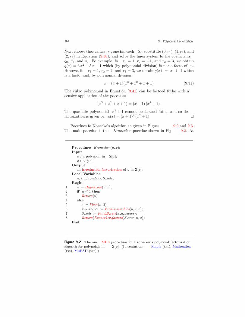
364 9. Polynomial Factorization
Next choose three values ri, one from each Si, substitute (0, r1), (1, r2), and(2, r2) in Equation (9.30), and solve the linear system for the coefficientsq0, q1, and q2. For example, for r1 = 1, r2 = −1, and r3 = 3, we obtainq(x) = 3 x2 − 5 x + 1 which (by polynomial division) is not a factor of u.However, for r1 = 1, r2 = 2, and r3 = 3, we obtain q(x) = x + 1 whichis a factor, and, by polynomial division
u = (x+ 1)(x3 + x2 + x+ 1). (9.31)
The cubic polynomial in Equation (9.31) can be factored further with arecursive application of the process as
(x3 + x2 + x+ 1) = (x+ 1) (x2 + 1).
The quadratic polynomial x2 + 1 cannot be factored further, and so thefactorization is given by u(x) = (x+ 1)2 (x2 + 1). �
Procedures for Kronecker’s algorithm are given in Figures 9.2 and 9.3.The main procedure is the Kronecker procedure shown in Figure 9.2. At
Procedure Kronecker (u, x);Input
u : a polynomial in Z[x];x : a symbol;
Outputan irrreducible factorization of u in Z[x];
Local Variablesn, s, x u values ,S sets ;
Begin1 n := Degree gpe(u, x);2 if n ≤ 1 then3 Return(u)4 else5 s := Floor(n/2);6 x u values := Find x u values(u, s, x);7 S sets := Find S sets(x u values);8 Return(Kronecker factors(S sets, u, x))
End
Figure 9.2. The main MPL procedure for Kronecker’s polynomial factorizationalgorithm for polynomials in Z[x]. (Implementation: Maple (txt), Mathematica(txt), MuPAD (txt).)

9.2. Irreducible Factorization: The Classical Approach 365
Procedure Kronecker factors(S sets, u, x);Input
u : a polynomial in Z[x];S sets : a list of lists of the form [xi, Si] where Si is
the set of positive and negative divisors of u(xi);x : a symbol;
Outputan irrreducible factorization of u in Z[x];
Local Variables c,m,N, i, j, S, points,X, q, v, k, w, g, p;Begin
1 N := 1;2 for i := 1 to Number of operands(S sets) do3 c[i] := 1;4 m[i] := Number of operands(Operand(Operand(S sets, i), 2));5 N := N ∗m[i];6 k := 1;7 while k ≤ N do8 points := [ ];9 for j := 1 to Number of operands(S sets) do10 w := Operand(S sets , j);11 X := Operand(w, 1);12 S := Operand(w, 2);13 points := Adjoin([X,Operand(S, c[j])], points);14 q := Lagrange polynomial(points, x);15 if Degree gpe(q, x) > 0 then16 g := Polynomial division(u, q, x);17 if Operand(g, 2) = 0 then18 v := Operand(g, 1);19 p := Find integer factors(q, v, x);20 Return(Kronecker(Operand(p, 1), x)
∗Kronecker(Operand(p, 2), x));21 j := 1;22 while j ≤ Number of operands(S sets) do23 if c[j] < m[j] then24 c[j] := c[j] + 1;25 j := Number of operands(S sets) + 126 else27 c[j] := 1; j := j + 1;28 k := k + 1;29 Return(u)
End
Figure 9.3. The MPL Kronecker factors procedure. (Implementation: Maple(txt), Mathematica (txt), MuPAD (txt).)

366 9. Polynomial Factorization
line 6, the procedure Find x u values obtains a list of lists
[[x1, u(x1)], . . . , [xs+1, u(xs+1)]], (9.32)
where xi is an integer and u(xi) �= 0. At line 7, the procedure Find S setsobtains another list
[[x1, S1], . . . , [xs+1, Ss+1]] (9.33)
where Si is the set of positive and negative divisors of u(xi). The detailsof both of these procedures are left to the reader (Exercises 4 and 5).
The Kronecker factors procedure, which is the heart of the algorithm,is invoked at line 8. This procedure is given in Figure 9.3. The proceduresearches for a factor of u by choosing, in a systematic way, values ui fromthe sets Si and creating and testing a trial factor that passes through thepoints
[[x1, u1], . . . , [xs+1, us+1]].
The array c[i], i = 1, 2, . . . , s+ 1 keeps track of which divisor is selectedfrom each Si, while the array m[i] contains the number of divisors in Si.Both of these arrays are given values in lines 2–5. Since each c[i] is initial-ized to 1, the first trial factor passes through the point [xi,Operand(Si, 1)]for 1 ≤ i ≤ s + 1. The variable N , which contains the number of ways atrial factor can be chosen, is also initialized in this loop.
The main loop of the procedure is given in lines 7–28. In lines 8–13,we construct a list called points that is used to find a trial divisor q inline 14. (The Lagrange polynomial procedure is described in Exercise 6.)In lines 15–17, we check if q is a divisor with positive degree and, if so,divide q into u at line 16. If the remainder of this division is 0 (line 17),then v is the quotient (line 18). Since q and v may have coefficients thatare not integers, at line 19 we first find the equivalent factors with integercoefficients using the Find integer factors procedure (Exercise 3), and thenapply the Kronecker procedure recursively to the new polynomials andreturn the product of the factors (line 20). In lines 21–29, we incrementthe c[j] values and j in preparation for trying another trial factor q. Ifwe complete the main loop without finding a divisor, then we return theirrreducible polynomial u (line 29).
Computational Efficiency of Kronecker’s Algorithm
Although Kronecker’s algorithm shows that polynomial factorization is analgorithmic process, it is notoriously slow. In fact, the algorithm is onlypractical for low degree polynomials with small coefficients, since in othercases the number of trial factors is prohibitively large.

9.2. Irreducible Factorization: The Classical Approach 367
Since polynomial factorization is such an important operation for com-puter algebra, it has attracted the attention of research mathematicians andcomputer scientists who have developed a number of more efficient (andmuch more involved) approaches to the problem. We describe a modernfactorization algorithm in Section 9.4.
Kronecker’s Algorithm for Multivariate Polynomials
Kronecker’s algorithm has a natural extension to multivariate polynomialswhich we illustrate with an example.
Example 9.19. Consider the polynomial
u(x, y) = 3 x y − y x3 − x2 + 2 x+ xy2 + x2 y + y2 x2.
Let’s first express u(x, y) as a polynomial in y with coefficients that arepolynomials in x:
u(x, y) =(2 x− x2
)+(3 x+ x2 − x3
)y +
(x+ x2
)y2.
We can simplify the process with
cont(u, y) = gcd(2 x− x2, 3 x+ x2 − x3, x+ x2
)= x
and the preliminary factorization
u = cont(u, y) pp(u, y) = x · ((2 − x) +(3 + x− x2
)y + (1 + x)y2
).
(9.34)In this case, cont(u, y) is irrreducible. If this were not so, it could befactored with the univariate version of Kronecker’s algorithm.
Let
w(x, y) = pp(u, y) =((2 − x) +
(3 + x− x2
)y + (1 + x)y2
).
Observe that w(x, y) is a quadratic in y, and so, if it can be factored, bothof the factors must be linear in y. Let
q(x, y) = m(x) y + b(x) (9.35)
be one of the linear factors, and suppose that
w(x, y) = q(x, y) v(x, y)
where v(x, y) is also linear in y. To find the two coefficients m(x) and b(x),we imitate what was done in the univariate case, but now the unknown
368 9. Polynomial Factorization
coefficients are polynomials in x. To do this, we need to find the valuesof q(x, y) at two values y = y1 and y = y2, and then, by substituting(y1, q(x, y1)) and (y2, q(x, y2)) into Equation (9.35), we obtain two linearequations for the two unknown polynomials m(x) and b(x). We use w(x, y)to find the two y values and the corresponding q(x, y) values.
As in the univariate case, we need two y values with w(x, y) �= 0. Inthis case,
w(x, 0) = 2− x, w(x, 1) = 6 + x− x2
will do. Since q(x, y) is a divisor of w(x, y), we must find all the divisors ofw(x, 0) and w(x, 1). Since these expressions are polynomials in x, we canfind the divisors of these polynomials by first factoring them (using Kro-necker’s algorithm for univariate polynomials) and then finding all divisorsof the polynomials (Exercise 12, page 125). Therefore,
q(x, 0) ∈ S1 = {±1, ± (2 − x)},q(x, 1) ∈ S2 = {±1, ± (2 + x), ± (3 − x), ± (2 + x) (3 − x)}.
To find a trial factor q(x, y), we choose an expression r1 from S1 and anexpression r2 from S2. Therefore, substituting
y = 0, q(x, y) = r1
andy = 1, q(x, y) = r2
into Equation (9.34), we obtain two equations for m(x) and b(x). If thesolution q(x, y) is a divisor of w(x, y), then q(x, y) is a factor. If not werepeat the process with other values for u1 and u2. For example, if wechoose
r1 = 2− x, r2 = 3− x,
we obtain the two equations
2− x = m(x) · 0 + b(x), 3− x = m(x) · 1 + b(x).
Solving these equations we obtain b(x) = 2 − x and m(x) = 1, and so atrial factor is q(x, y) = y + (2 − x). In this case q(x, y) is a factor, and bydividing q(x, y) into w(x, y) we obtain the factorization
w(x, y) = (y + 2− x) (x y + y + 1).
Therefore, using Equation (9.34), the original polynomial u(x, y) can befactored as
u(x, y) = x (y + 2− x) (x y + y + 1). �

9.2. Irreducible Factorization: The Classical Approach 369
Exercises1. Factor each of the following using Kronecker’s algorithm.
(a) x3 + 2x2 + 2x + 1
(b) x3 + x2 + x + 1
2. Use Kronecker’s algorithm to show that u = x2 + 1 cannot be factored inZ[x].
3. Let u be a polynomial in Z[x], and let u = v w be a factorization in termsof rational coefficients. Give a procedure
Find integer factors(v, w, x)
that returns a list [v1, w1] where u = v1 · w1 is a factorization in Z[x].
4. Let u be a polynomial in Z[x] with positive degree, x a symbol, and s > 0an integer. Give a procedure
Find x u values(u, x, s)
that returns the list (9.32), where xi is an integer and u(xi) �= 0.
5. Let L be a list of the form (9.32). Give a procedure
Find S sets(L)
that returns the list (9.33). (Exercise 6 on page 34 is useful in this exercise.)
6. Let P = [[x1, y1], . . . , [xr+1, yr+1]] be a list of 2 element lists, where xi
and yi are rational numbers. The Lagrange interpolation polynomial thatpasses through these points is given by
L(x) =
r+1
i=1
yiLi(x).
where
Li(x) =(x− x1) · · · (x− xi−1)(x− xi+1) · · · (x− xr+1)
(xi − x1) · · · (xi − xi−1)(xi − xi+1) · · · (xi − xr+1).
Give a procedure Lagrange polynomial(P, x) that returns the polynomialL(x). For example,
Lagrange polynomial([[1, 1], [2,−1]], x) → −2x + 3.
7. Give a procedure
Find Z poly(u, x)
that returns the list [cont(v)/M, pp(v)] where M is given by Equation(9.23) and v is given by Equation (9.24).

370 9. Polynomial Factorization
8. Give a procedure
Factor sv(u, x)
that finds the irrreducible factorization of a polynomial u in Q[x]. (The suf-fix “sv” stands for “single variable.”) First, find a square-free factorizationof u in Q[x]. Then, use Kronecker’s algorithm to factor the primitive partof the integer-coefficient version of each square-free factor of u (see Equa-tions (9.23)-(9.26)). (Exercise 7 is useful in this exercise.)
In Exercise 18 on page 429, we suggest a modification of this procedure thatfinds the irrreducible factorization in Z[x] using the approach described inSection 9.4.
9. Use Kronecker’s algorithm to factor u = y2 + x y + y + x.
9.3 Factorization in Zp[x]
Let p > 1 be a prime number. In this section we describe an algorithmthat finds the irrreducible factorization of a polynomial u in Zp[x]. First,we obtain a square-free factorization of u by using a modification of theapproach described in Section 9.1, and then complete the process by findingthe irrreducible factorization of each of the square-free factors. Since thefinite field Zp has a richer algebraic structure than the infinite integraldomain Z, the irrreducible factorization problem is simpler in Zp[x] thanin Z[x].
Although the factorization problem in Zp[x] is important in its ownright, we introduce it here because it plays an essential role in the factor-ization algorithm in Z[x].Notation Convention. In this section, to simplify the notation, we
use the ordinary algebraic operators (+ and ·) for addition and multiplica-tion of polynomials rather than the more cumbersome notation ⊕p and ⊗pintroduced for Zp in Section 2.3. For example, for u(x) and v(x) in Zp[x],u(x) + v(x) refers to the addition of polynomials where the arithmetic ofcorresponding coefficients of the polynomials is performed in Zp.
Algebraic Relationships in Zp[x]
We begin by describing a number of algebraic relationships that apply topolynomials in Zp[x].
Theorem 9.20. Let p > 1 be a prime number. Then, in Zp[x],
xp − x = x (x− 1) · · · (x− (p− 2)) (x − (p− 1)). (9.36)

9.3. Factorization in Zp[x] 371
Proof: By Fermat’s little theorem (Theorem 2.43(3), page 54), each b inZp is a root of xp − x = 0. Since both sides of Equation (9.36) are monicand have the same degree and roots, the relationship follows. �
The relationship in the next theorem is the polynomial version of Theo-rem 2.43(2) on page 54. The proof is similar to the proof for that theorem.
Theorem 9.21. Let p > 1 be a prime number, and let u(x) and v(x) bepolynomials in Zp[x]. Then, (u(x) + v(x))p = u(x)p + v(x)p. �
The relationship in the next theorem plays a key role in the developmentof both the square-free and irrreducible factorization algorithms in Zp[x].
Theorem 9.22. Let p > 1 be a prime number, and let u(x) be in Zp[x].Then, u(x)p = u(xp).
Proof: The proof uses mathematical induction on n = deg(u). For n = 0,the polynomial u is a constant, and so the theorem follows from Fermat’slittle theorem (page 54). Suppose that n > 0, and assume the inductionhypothesis that the theorem holds for polynomials with degree ≤ n − 1.We have
u(x) = unxn + v(x)
where v represents all the terms in u(x) that have degree ≤ n − 1. UsingTheorem 9.21 and the induction hypothesis applied to v, we have
u(x)p = (unxn + v(x))p = (unxn)p + v(x)p
= upn · (xn)p + v(xp) = un · (xp)n + v(xp)= u(xp). �
Square-Free Factorization Algorithm in Zp[x]In Section 9.1 we described an algorithm that obtains the square-freefactorization for polynomials in F[x] when the field F contains the inte-gers. In that setting, both the mathematics and the algorithm use theproperty that a polynomial with positive degree cannot have a zero deriva-tive (Theorem 9.4, page 351). Since this property does not hold for allpolynomials in Zp[x] (e.g., for p = 3, (x3 + 1)′ = 0), the mathematical de-velopment and algorithm must be modified. Fortunately, there is a simpleway to describe polynomials in Zp[x] which have a zero derivative.
Theorem 9.23. Let p > 1 be a prime number, and let u be a polynomial inZp[x]. Then, u′ = 0 if and only if u = f(xp), where f(x) is in Zp[x].
372 9. Polynomial Factorization
Proof: If u = f(xp), then p divides the coefficient of each monomial in thederivative, and so u′ = 0. Conversely, suppose that u = anx
n + · · · + a0
and u′ = 0. This implies that p divides the coefficient of each monomialai i x
i−1 of u′, and since p is a prime, by Theorem 2.16(2), we have p|ai orp|i. If p|ai, then since 0 ≤ ai ≤ p− 1, we have ai = 0. On the other hand,if p|i, the monomial in u has the form ai(xp)q where q = iquot(i, p). Sinceeach non-zero monomial has this form, u has the form f(xp). �
Using the last theorem and Theorem 9.22, we obtain the analogue ofTheorem 9.5 in Zp[x].
Theorem 9.24. Let p > 1 be a prime number, and let u be a polynomial inZp[x]. Then, u is square-free if and only if gcd(u, u′) = 1.
Proof: The proof is similar to the one for Theorem 9.5 (page 351), withthe following modification to the second half of the proof when u has afactor with positive degree and zero derivative. As in the earlier proof,suppose that u = q1 v with deg(v) > 0, but now suppose that v′ = 0.Then, by Theorems 9.22 and 9.23, v = (f(x))p, which implies that u is notsquare-free. With this observation added to the proof of Theorem 9.5, weobtain a proof of the present theorem. �
Suppose now that u has the square-free factorization
u = c∏
1≤i≤msii (9.37)
where the polynomials si are monic, square-free, and relatively prime. Analgorithm that obtains this factorization is similar to the one given in Sec-tion 9.1 with a modification that accounts for the possibility that some ofthe square-free factors may have zero derivative. Let
v =∏
1 ≤ i ≤ ms′i = 0
sii, w =∏
1 ≤ i ≤ ms′i = 0
sii,
where v and w are monic and
u = c v w. (9.38)
Since w′ = 0, we have u′ = c v′ w, and since each square-free factor of vhas non-zero derivative, gcd(v, v′) is obtained with manipulations similarto those given in Section 9.1. Therefore (using Exercise 11, page 144),

9.3. Factorization in Zp[x] 373
gcd(u, u′) = gcd(c v w, c v′ w)= w gcd(v, v′) (9.39)
= w∏
2 ≤ i ≤ ms′i = 0
si−1i .
A procedure that obtains the square-free factorization in Zp[x] is similarto the one in Figure 9.1 (page 356) with three modifications. The followingdiscussion refers to the variables in this procedure.
First, Equation (9.39) shows that the variable R assigned at line 6 ofthis procedure has w as a factor. In addition, this factor is not removedfrom R by the manipulations in the loop (lines 10–15). To see why, supposethat at line 4, U = v w. Then at lines 6–7,
R = w gcd(v, v′), F =U
R=
v
gcd(v, v′).
In addition, in the while loop that begins at line 9, G at line 10 does nothave w as a factor, and so R at line 13 does have w as a factor. Therefore,if line 9 is replaced by
while Derivative(R, x) �= 0 do,
then at line 16, P contains the square-free factorization of v and R = w.The secondmodification of the procedure obtains the square-free factorization
of w. By Theorems 9.22 and 9.23, we can represent w as
w(x) = f(xp) = f(x)p, (9.40)
where f(x) is obtained by substituting x1/p for x in w. We obtain thesquare-free factorization of f with a recursive application of the procedureand then obtain the factorization for w by taking the factorization for f tothe power p.
Finally, the square-free factorization for u is obtained using the factor-izations for v and w and Equation (9.38). The details of the procedure areleft to the reader (Exercise 1).
Irreducible Factorization of Square-Free Polynomials in Zp[x]To complete the factorization problem, we must obtain the irrreduciblefactorization of each of the monic, square-free polynomials si in Equa-tion (9.37).
Let u be a monic square-free polynomial in Zp[x] with n = deg(u). Asimple approach to the factorization problem is obtained by mimicking the

374 9. Polynomial Factorization
trial-factors approach used by Kronecker’s algorithm. If u is reducible, itmust have a monic factor of degree m with 1 ≤ m ≤ iquot(n, 2), and sinceZp is finite, there are a finite number of trial polynomials of this type.Using polynomial division, we check each trial polynomial (starting withpolynomials of degree 1), and if a factor f is found, we obtain the completefactorization by applying the algorithm recursively to quot(u,f). If none ofthe trial polynomials is a factor, then u is irrreducible.
Although, the approach is not difficult to implement (Exercise 10), likeKronecker’s algorithm, it is highly inefficient. Indeed, the number of trialfactors is given by
piquot(n,2)+1 − p
p− 1
which is large even for small values of p (Exercise 2). For example, for p =11 and n = 16, there are 235, 794, 768 trial factors with degree 1 ≤ m ≤ 8.There has got to be a better way!
A better approach is an algorithm, discovered in the late 1960s by E.R. Berlekamp, that obtains the factorization by reducing the problem tothe solution of a system of linear equations followed by a number of gcdcalculations.
Auxiliary Polynomials
The first step in the development of the algorithm is the formal definitionof the auxiliary polynomials that are used in the gcd calculations. TheChinese remainder theorem (Theorem 4.41, page 140) plays a central rolehere since it guarantees (in a theoretical sense) the existence of these poly-nomials. However, the Chinese remainder procedure that finds the solutionto the remainder equations has no computational role in the algorithm.
The auxiliary polynomials are defined in the following way. Let u(x) bea monic and square-free polynomial in Zp[x] with an irrreducible factorization
u = u1 · · · ur, (9.41)
where each ui is monic and has positive degree. Suppose that a1, . . . , arare in Zp, and consider the polynomial h(x) that satisfies the system ofremainder equations and degree condition
rem(h(x), ui) = ai for 1 ≤ i ≤ r, deg(h) < deg(u). (9.42)
Since u is square-free, the ui are distinct, and so the Chinese remaindertheorem guarantees that there is a unique h(x) that satisfies these condi-tions.
9.3. Factorization in Zp[x] 375
Example 9.25. Suppose that p = 5 and u = x6 + x5 + x + 4. Using thealgorithm described later in this section, the irrreducible factorization foru in Z5[x] is given by
u = u1 u2 u3 = (x2 + x+ 2) (x2 + 2 x+ 3) (x2 + 3 x+ 4).
Each choice of a1, a2, and a3 gives a unique polynomial h(x). For example,if a1 = 1, a2 = 2, and a3 = 3, then using the algorithm suggested in theproof of the Chinese remainder theorem, we have
h = 4 x5 + 4 x. (9.43)
In a similar way, if a1 = 1, a2 = 1, and a3 = 2, then
h = 2 x5 + x4 + 4 x3 + 4 x2 + 2 x+ 1. (9.44)
Finally, if a1 = 1, a2 = 1, and a3 = 1, then
h = 1. (9.45)
�
The next theorem gives two important properties of the auxiliary poly-nomials h(x).
Theorem 9.26. Let p > 1 be a prime number, and let u(x) be a monic,square-free polynomial in Zp[x] with the irrreducible factorization
u = u1 · · ·ur.
1. There are pr distinct polynomials h(x) that satisfy the remainderequations (9.42) where each sequence a1, . . . , ar gives a unique h(x).
2. For each h(x) that satisfies the remainder equations (9.42),
u(x) =p−1∏j=0
gcd(u(x), h(x) − j) (9.46)
where the factors in the product are relatively prime.
Proof: To show (1), for each sequence a1, a2, . . . , ar, the Chinese remaindertheorem shows that there is a unique h(x) that satisfies the remainderequations (9.42). In addition, since 0 ≤ ai ≤ p − 1, there are pr such
376 9. Polynomial Factorization
sequences, and since each sequence gives a distinct polynomial, there arepr such polynomials.
To show (2), first observe that the factors in Equation (9.46) are rela-tively prime since the polynomials h(x)−j, j = 0, 1, . . . , p−1 are relativelyprime (Exercise 11, page 125). Since both sides of Equation (9.46) aremonic, we need only show that each side divides the other side. Let
H(x) =p−1∏j=0
gcd(u(x), h(x) − j).
Since h(x) satisfies the remainder equations (9.42), each irrreducible fac-tor ui of u divides some h(x) − j, which implies that each ui|H(x). Inaddition, since the polynomials u1, . . . , ur are relatively prime, Theorem4.29(3) (page 133) implies that u(x)|H(x). On the other hand, each of therelatively prime factors of H(x) divides u(x), and so H(x)|u(x). Therefore,we obtain Equation (9.46). �
The relationship in Equation (9.46) shows that the auxiliary polynomi-als provide a way to obtain a factorization using gcd calculations. However,for some j, the expression gcd(u(x), h(x)− j) may be 1, and for other j, itmay be reducible. Both of these points are illustrated in the next example.
Example 9.27. Suppose that p = 5, and consider the polynomial
u = x6 + x5 + x+ 4
in Zp[x] from Example 9.25. Using the h in Equation (9.43) and the pro-cedure Poly div p (Exercise 9, page 125), the factorization in Equation(9.46) is
u = 1 · (x2 + x+ 2) (x2 + 2 x+ 3) (x2 + 3 x+ 4) · 1.In this case, we obtain all three irrreducible factors of u. However, usingthe h in Equation (9.44), we obtain
u = 1 · 1 · (x4 + 3 x3 + 2 x2 + 2 x+ 1) (x2 + 3 x+ 4) · 1.In this case, two of the irrreducible factors of u coalesce into one factor.Finally, using the h given in Equation (9.45),
u = 1 · (x6 + x5 + x+ 4) · 1 · 1 · 1.In this case, Equation (9.46) does not obtain any of the irrreducible factorsof u. �
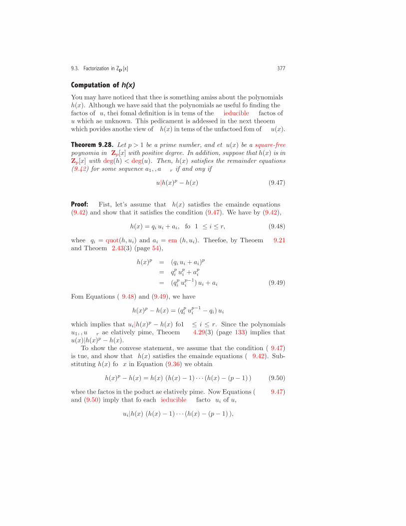
9.3. Factorization in Zp[x] 377
Computation of h(x)You may have noticed that there is something amiss about the polynomialsh(x). Although we have said that the polynomials are useful for finding thefactors of u, their formal definition is in terms of the irrreducible factors ofu which are unknown. This predicament is addressed in the next theoremwhich provides another view of h(x) in terms of the unfactored form of u(x).
Theorem 9.28. Let p > 1 be a prime number, and let u(x) be a square-freepolynomial in Zp[x] with positive degree. In addition, suppose that h(x) is inZp[x] with deg(h) < deg(u). Then, h(x) satisfies the remainder equations(9.42) for some sequence a1, . . . , ar if and only if
u|h(x)p − h(x). (9.47)
Proof: First, let’s assume that h(x) satisfies the remainder equations(9.42) and show that it satisfies the condition (9.47). We have by (9.42),
h(x) = qi ui + ai, for 1 ≤ i ≤ r, (9.48)
where qi = quot(h, ui) and ai = rem(h, ui). Therefore, by Theorem 9.21and Theorem 2.43(3) (page 54),
h(x)p = (qi ui + ai)p
= qpi upi + api
= (qpi up−1i )ui + ai. (9.49)
From Equations (9.48) and (9.49), we have
h(x)p − h(x) = (qpi up−1i − qi)ui
which implies that ui|h(x)p − h(x) for 1 ≤ i ≤ r. Since the polynomialsu1, . . . , ur are relatively prime, Theorem 4.29(3) (page 133) implies thatu(x)|h(x)p − h(x).
To show the converse statement, we assume that the condition (9.47)is true, and show that h(x) satisfies the remainder equations (9.42). Sub-stituting h(x) for x in Equation (9.36) we obtain
h(x)p − h(x) = h(x) (h(x) − 1) · · · (h(x)− (p− 1) ) (9.50)
where the factors in the product are relatively prime. Now Equations (9.47)and (9.50) imply that for each irrreducible factor ui of u,
ui|h(x) (h(x) − 1) · · · (h(x) − (p− 1) ),

378 9. Polynomial Factorization
and since ui is irrreducible, it divides exactly one factor on the right of thisexpression. Let ai be the member of Zp determined by this factor. There-fore, ui|h− ai for i = 1, . . . , r, and the uniqueness property for polynomialdivision implies that h satisfies the remainder equations rem(h, ui) = ai. �
A Linear System of Equations for h(x)We show next how the alternate description of h in Theorem 9.28 is usedto obtain a system of (dependent) linear equations which has as solutionsall the auxiliary polynomials h(x).
Let n = deg(u) ≥ 1. Since deg(h) < n, each h(x) has the form
h(x) = h0 + h1x+ · · ·+ hn−1xn−1. (9.51)
Let’s set up a system of equations for the coefficients of h. First, byTheorem 9.22,
h(x)p = h(xp) =n−1∑j=0
hjxp j ,
and
h(x)p − h(x) =n−1∑j=0
hj (xp j − xj). (9.52)
By polynomial division,
xp j = Qj(x)u(x) + rj(x) (9.53)
where deg(rj(x)) ≤ n−1. Substituting this expression into Equation (9.52),we have
h(x)p − h(x) =n−1∑j=0
hj (Qj(x)u(x) + rj(x)− xj)
=
n−1∑j=0
hj Qj(x)
u(x) +
n−1∑j=0
hj (rj(x) − xj).
Observe that the sum on the far right has degree < n, and therefore, usingthe condition (9.47) and the uniqueness property of polynomial division,we have
0 = rem(h(x)p − h(x), u(x)) =n−1∑j=0
hj (rj(x)− xj). (9.54)

9.3. Factorization in Zp[x] 379
Now, suppose that
rj(x) =n−1∑i=0
rijxi, (9.55)
and let
δij ={0, i �= j,1, i = j.
Substituting Equation (9.55) into Equation (9.54), we obtain
0 =n−1∑j=0
hj
(n−1∑i=0
(rijx
i)− xj
)
=n−1∑j=0
hj
(n−1∑i=0
(rijx
i − δijxi))
=n−1∑i=0
n−1∑j=0
hj (rij − δij)
xi,
where in the last sum the coefficient of each xi is 0. This gives the followingsystem of n linear equations for the coefficients of h(x):
n−1∑j=0
hj (rij − δij) = 0, i = 0, 1, . . . , n− 1.
In matrix form the system of equations is
R h = 0, (9.56)
where
R =
∣∣∣∣∣∣∣∣∣r0,0 − 1 r0,1 · · · r0,(n−1)r1,0 r1,1 − 1 · · · r1,(n−1)
......
...r(n−1),0 r(n−1),1 · · · r(n−1),(n−1) − 1
∣∣∣∣∣∣∣∣∣(9.57)
and
h =
∣∣∣∣∣∣∣∣∣h0
h1
...hn−1
∣∣∣∣∣∣∣∣∣, 0 =
∣∣∣∣∣∣∣∣∣00...0
∣∣∣∣∣∣∣∣∣. (9.58)
The system of equations (9.56) is not independent. For one thing, sincedeg(u) > 0, r0(x) = rem(xp·0, u) = 1, and so all entries in the first column
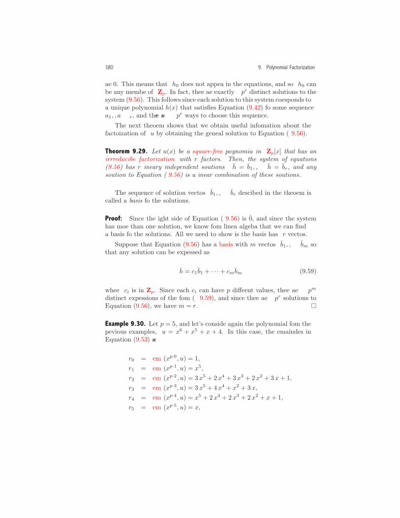
380 9. Polynomial Factorization
are 0. This means that h0 does not appear in the equations, and so h0 canbe any member of Zp. In fact, there are exactly pr distinct solutions to thesystem (9.56). This follows since each solution to this system corresponds toa unique polynomial h(x) that satisfies Equation (9.42) for some sequencea1, . . . , ar, and there are pr ways to choose this sequence.
The next theorem shows that we obtain useful information about thefactorization of u by obtaining the general solution to Equation (9.56).
Theorem 9.29. Let u(x) be a square-free polynomial in Zp[x] that has anirrreducible factorization with r factors. Then, the system of equations(9.56) has r linearly independent solutions h = b1, . . . , h = br, and anysolution to Equation (9.56) is a linear combination of these solutions.
The sequence of solution vectors b1, . . . , br described in the theorem iscalled a basis for the solutions.
Proof: Since the right side of Equation (9.56) is 0, and since the systemhas more than one solution, we know from linear algebra that we can finda basis for the solutions. All we need to show is the basis has r vectors.
Suppose that Equation (9.56) has a basis with m vectors b1, . . . , bm sothat any solution can be expressed as
h = c1b1 + · · ·+ cmbm (9.59)
where ci is in Zp. Since each ci can have p different values, there are pm
distinct expressions of the form (9.59), and since there are pr solutions toEquation (9.56), we have m = r. �
Example 9.30. Let p = 5, and let’s consider again the polynomial from theprevious examples, u = x6 + x5 + x + 4. In this case, the remainders inEquation (9.53) are
r0 = rem(xp·0, u) = 1,r1 = rem(xp·1, u) = x5,
r2 = rem(xp·2, u) = 3 x5 + 2 x4 + 3 x3 + 2 x2 + 3 x+ 1,r3 = rem(xp·3, u) = 3 x5 + 4 x4 + x2 + 3 x,r4 = rem(xp·4, u) = x5 + 2 x4 + 2 x3 + 2 x2 + x+ 1,r5 = rem(xp·5, u) = x,

9.3. Factorization in Zp[x] 381
which gives
R =
∣∣∣∣∣∣∣∣∣∣∣∣
1− 1 0 1 0 1 00 0− 1 3 3 1 10 0 2− 1 1 2 00 0 3 0− 1 2 00 0 2 4 2− 1 00 1 3 3 1 0− 1
∣∣∣∣∣∣∣∣∣∣∣∣
=
∣∣∣∣∣∣∣∣∣∣∣∣
0 0 1 0 1 00 4 3 3 1 10 0 1 1 2 00 0 3 4 2 00 0 2 4 1 00 1 3 3 1 4
∣∣∣∣∣∣∣∣∣∣∣∣(9.60)
where all arithmetic is done in Z5[x]. Using an approach described later inthis section, a basis for the solutions is
b1 =
∣∣∣∣∣∣∣∣∣∣∣∣
100000
∣∣∣∣∣∣∣∣∣∣∣∣, b2 =
∣∣∣∣∣∣∣∣∣∣∣∣
004410
∣∣∣∣∣∣∣∣∣∣∣∣, b3 =
∣∣∣∣∣∣∣∣∣∣∣∣
010001
∣∣∣∣∣∣∣∣∣∣∣∣. (9.61)
Since the basis has three vectors, we know that u has three irrreduciblefactors. These solutions to Equation (9.56) correspond to the three linearlyindependent solutions to Equation (9.42):
b1(x) = 1, b2(x) = x4 + 4 x3 + 4 x2, b3(x) = x5 + x,
and any auxiliary polynomial h(x) is a linear combination of these polyno-mials. For example, h(x) in Equation (9.44) is given by
h = 2 x5 + x4 + 4 x3 + 4 x2 + 2 x+ 1 = 1 · b1 + 1 · b2 + 2 · b3. �
Separating the Factors of u(x) with Basis PolynomialsThe final step in the factorization process involves finding the irrreduciblefactors of u using the auxiliary polynomials h(x). The basic tool for thisfactorization is the relation in Equation (9.46) on page 375. However,as we saw in Example 9.27, for some h(x), Equation (9.46) may not ob-tain the complete irrreducible factorization. In fact, if u has more than

382 9. Polynomial Factorization
p factors, Equation (9.46) cannot obtain the complete factorization withone h(x), and so more than one auxiliary polynomial is needed. Thenext theorem and subsequent discussion show how the basis polynomialsb1(x), b2(x), . . . , br(x) can be used to separate the factors.
Theorem 9.31. Suppose that u is a square-free polynomial in Zp[x] withr ≥ 2 factors, and let ui and uj be two distinct irrreducible factors of u.
1. There is a basis polynomial bk(x) such that rem(bk, ui) �= rem(bk, uj).
2. There is an element d in Zp such that
ui|gcd(u, bk − d), uj /| gcd(u, bk − d)
where bk is obtained in Part (1) of the theorem.
Proof: To show (1), from the definition of the auxiliary polynomials, thereis an h that satisfies Equation (9.42) such that
rem(h, ui) = ai �= aj = rem(h, uj). (9.62)
In addition, we can represent h as
h = c1 b1 + · · ·+ cr br
where ci is in Zp. We claim that it is not possible to have
rem(bk, ui) = rem(bk, uj), 1 ≤ k ≤ r.
If this were so,
rem(h, ui) = c1 rem(b1, ui) + · · ·+ cr rem(br, ui)= c1 rem(b1, uj) + · · ·+ cr rem(br, uj)= rem(h, uj)
which contradicts the conditions in (9.62).To show (2), let bk be the polynomial obtained in Part (1), and let
d = rem(bk, ui). Then, ui|bk − d, which implies that ui|gcd(u, bk − d).Next, if uj|gcd(u, bk − d), then uj|bk − d, and the uniqueness property ofpolynomial division implies that rem(bk, uj) = d which contradicts Part(1) of the theorem. �
Theorem 9.31(2) gives a way to determine each factor ui of u. Thetheorem implies that for each of the other factors
uj, j = 1, . . . , i− 1, i+ 1, . . . , r,

9.3. Factorization in Zp[x] 383
there is a basis polynomial bθ(j) in {b1, . . . , br} and an element dj in Zpsuch that
ui|gcd(u, bθ(j) − dj), uj /| gcd(u, bθ(j) − dj), (9.63)
for j = 1, . . . , i − 1, i+ 1, . . . , r. (The function notation θ(j) indicates thechoice of the basis polynomial depends on the factor uj.) If we let
ej = gcd(u, bθ(j) − dj), (9.64)
thenui = gcd(e1, . . . , ei−1, ei+1, . . . , er). (9.65)
Indeed, by (9.63), ui divides all the ej , and so it divides the gcd on theright. However, since
gcd(e1, . . . , ei−1, ei+1, . . . , er)|ej |u,
and since no other factor of u divides all the ej , we obtain Equation (9.65).The relationship in Equation (9.65) is important in a theoretical sense
because it shows that by performing a sufficient number gcd calculationsof the form
gcd(u, bk − j), k = 1, . . . , r, j = 0, . . . , p− 1,
we have enough information to obtain each factor of u. However, theformula is not useful in a computational sense because it overstates thework required. Later in this section, we give an algorithm that obtains thefactorization from the basis polynomials.
Procedures for Berlekamp’s Algorithm
Let u be a square-free and monic polynomial in Zp[x]. Berlekamp’s algo-rithm obtains the irrreducible factorization of u using the following threesteps.
1. Find the matrix R.
2. Using the matrix R, find a list S = [b1, . . . , br] that contains a basisof auxiliary polynomials. When there are r polynomials in S, thepolynomial u has r irrreducible factors.
3. Use the basis polynomials in S to find the irrreducible factors of u.

384 9. Polynomial Factorization
Procedure Berlekamp factor(u, x, p);Input
u : a monic, square-free polynomial in Zp[x];x : a symbol;p : a prime > 1;
OutputThe set of irrreducible factors of u;
GlobalR : an n by n matrix with entries in Zp;
Local Variablesn, S;
Begin1 n := Degree gpe(u, x);2 if n = 0 or n = 1 thenReturn({u})3 else4 R matrix(u, x, n, p);5 S := Auxiliary basis(x, n, p);6 if Number of operands(S) = 1 then7 Return({u})8 else9 Return(Find factors(u, S, x, p))
End
Procedure R matrix(u, x, n, p);Input
u : a monic, square-free polynomial in Zp[x];x : a symbol;n : a positive integer representing deg(u);p : a prime > 1;
OutputCreates the global matrix R
GlobalR : an n by n matrix with entries in Zp;
The body of the procedure is left to the reader (Exercise 5).
Figure 9.4. The MPL procedure Berlekamp factor and the heading of the pro-cedure R matrix in Berlekamp’s algorithm. The Berlekamp factor procedurereturns the set of irrreducible factors of u. (Implementation: Maple (txt),Mathematica (txt), MuPAD (txt).)
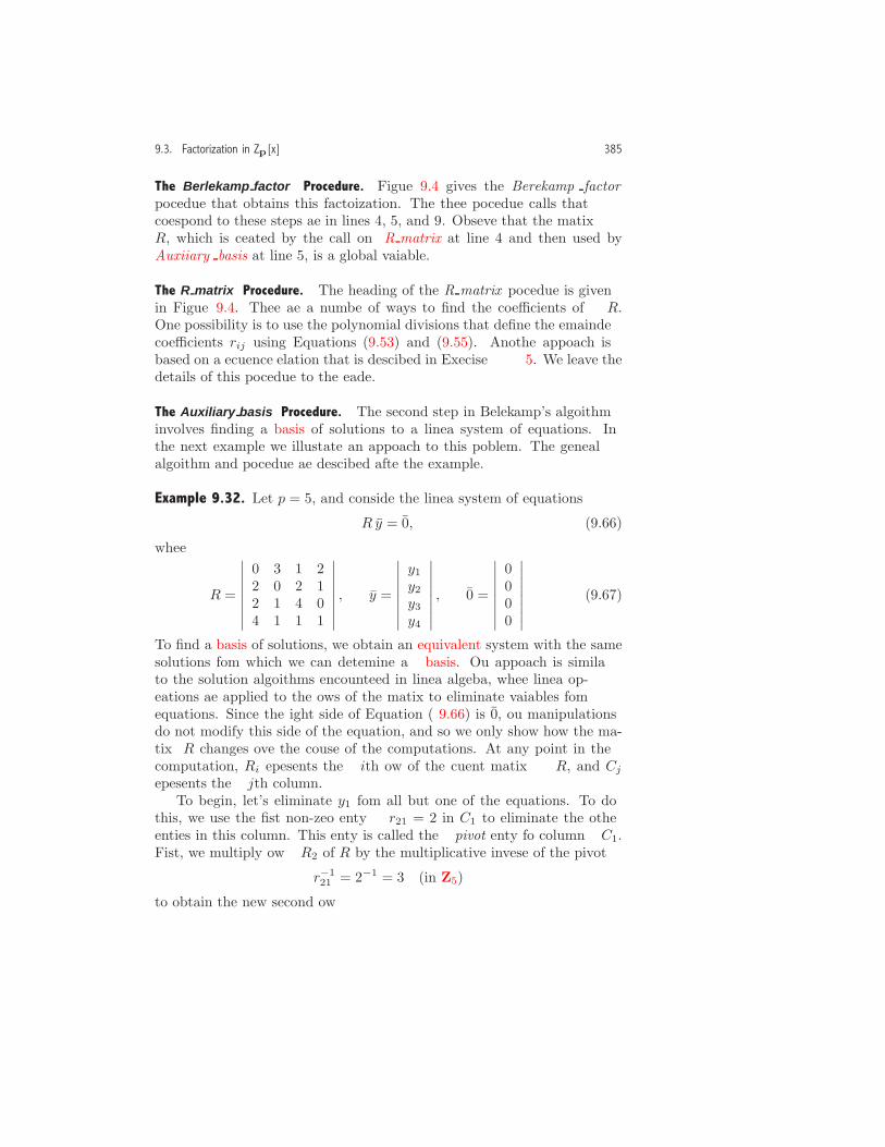
9.3. Factorization in Zp[x] 385
The Berlekamp factor Procedure. Figure9.4 gives the Berlekamp factorprocedure that obtains this factorization. The three procedure calls thatcorrespond to these steps are in lines 4, 5, and 9. Observe that the matrixR, which is created by the call on R matrix at line 4 and then used byAuxiliary basis at line 5, is a global variable.
The R matrix Procedure. The heading of the R matrix procedure is givenin Figure 9.4. There are a number of ways to find the coefficients of R.One possibility is to use the polynomial divisions that define the remaindercoefficients rij using Equations (9.53) and (9.55). Another approach isbased on a recurrence relation that is described in Exercise 5. We leave thedetails of this procedure to the reader.
The Auxiliary basis Procedure. The second step in Berlekamp’s algorithminvolves finding a basis of solutions to a linear system of equations. Inthe next example we illustrate an approach to this problem. The generalalgorithm and procedure are described after the example.
Example 9.32. Let p = 5, and consider the linear system of equations
R y = 0, (9.66)
where
R =
∣∣∣∣∣∣∣∣0 3 1 22 0 2 12 1 4 04 1 1 1
∣∣∣∣∣∣∣∣ , y =
∣∣∣∣∣∣∣∣y1
y2
y3
y4
∣∣∣∣∣∣∣∣ , 0 =
∣∣∣∣∣∣∣∣0000
∣∣∣∣∣∣∣∣ . (9.67)
To find a basis of solutions, we obtain an equivalent system with the samesolutions from which we can determine a basis. Our approach is similarto the solution algorithms encountered in linear algebra, where linear op-erations are applied to the rows of the matrix to eliminate variables fromequations. Since the right side of Equation (9.66) is 0, our manipulationsdo not modify this side of the equation, and so we only show how the ma-trix R changes over the course of the computations. At any point in thecomputation, Ri represents the ith row of the current matrix R, and Cjrepresents the jth column.
To begin, let’s eliminate y1 from all but one of the equations. To dothis, we use the first non-zero entry r21 = 2 in C1 to eliminate the otherentries in this column. This entry is called the pivot entry for column C1.First, we multiply row R2 of R by the multiplicative inverse of the pivot
r−121 = 2−1 = 3 (in Z5)
to obtain the new second row
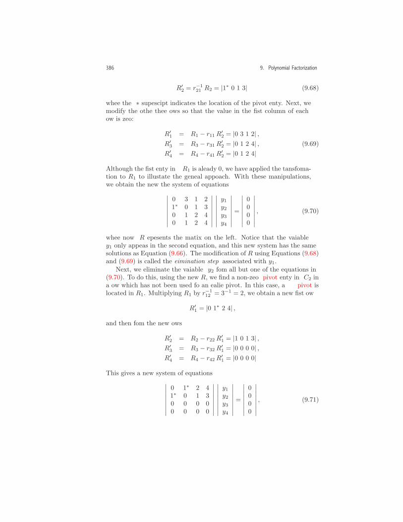
386 9. Polynomial Factorization
R′2 = r−1
21 R2 = |1∗ 0 1 3| (9.68)
where the ∗ superscript indicates the location of the pivot entry. Next, wemodify the other three rows so that the value in the first column of eachrow is zero:
R′1 = R1 − r11 R
′2 = |0 3 1 2| ,
R′3 = R3 − r31 R
′2 = |0 1 2 4| , (9.69)
R′4 = R4 − r41 R
′2 = |0 1 2 4| .
Although the first entry in R1 is already 0, we have applied the transforma-tion to R1 to illustrate the general approach. With these manipulations,we obtain the new the system of equations∣∣∣∣∣∣∣∣
0 3 1 21∗ 0 1 30 1 2 40 1 2 4
∣∣∣∣∣∣∣∣
∣∣∣∣∣∣∣∣y1
y2
y3
y4
∣∣∣∣∣∣∣∣ =∣∣∣∣∣∣∣∣0000
∣∣∣∣∣∣∣∣ , (9.70)
where now R represents the matrix on the left. Notice that the variabley1 only appears in the second equation, and this new system has the samesolutions as Equation (9.66). The modification of R using Equations (9.68)and (9.69) is called the elimination step associated with y1.
Next, we eliminate the variable y2 from all but one of the equations in(9.70). To do this, using the new R, we find a non-zero pivot entry in C2 ina row which has not been used for an earlier pivot. In this case, a pivot islocated in R1. Multiplying R1 by r−1
12 = 3−1 = 2, we obtain a new first row
R′1 = |0 1∗ 2 4| ,
and then form the new rows
R′2 = R2 − r22 R
′1 = |1 0 1 3| ,
R′3 = R3 − r32 R
′1 = |0 0 0 0| ,
R′4 = R4 − r42 R
′1 = |0 0 0 0| .
This gives a new system of equations∣∣∣∣∣∣∣∣0 1∗ 2 41∗ 0 1 30 0 0 00 0 0 0
∣∣∣∣∣∣∣∣
∣∣∣∣∣∣∣∣y1
y2
y3
y4
∣∣∣∣∣∣∣∣ =∣∣∣∣∣∣∣∣0000
∣∣∣∣∣∣∣∣ , (9.71)

9.3. Factorization in Zp[x] 387
where now R represents the matrix on the left. Notice that the variable y2
only appears in the first equation, and this system has the same solutionsas Equation (9.66).
Next, using the new R, we try to eliminate y3 from all but one equationby finding a pivot in C3. However, since the only non-zero entries in C3
are in rows that already contain pivots, we cannot find a pivot. Instead,this situation is an opportunity to construct the first member of the basis.Since there are now only two independent equations, we can assign valuesto two of the variables (say y3 = 1 and y4 = 0) and find a basis vector ofthe form
S3 =
∣∣∣∣∣∣∣∣y1
y2
10
∣∣∣∣∣∣∣∣ . (9.72)
The subscript 3 refers to the current column, and the two unknown valuesy1 and y2 are determined using the two non-zero equations in (9.71). (Wewill see below why this is a useful form.) Using the first equation in (9.71),we have y2 +2 = 0 or y2 = −2 = 3 (in Z5), and using the second equation,we have y1 + 1 = 0 or y1 = −1 = 4. Therefore, the first basis vector is
S3 =
∣∣∣∣∣∣∣∣4310
∣∣∣∣∣∣∣∣ . (9.73)
Finally, we try to find a pivot for y4, and again find that the only non-zero entries in C4 are in rows that already contain pivots. Instead, we finda second basis solution of the form
S4 =
∣∣∣∣∣∣∣∣y1
y2
01
∣∣∣∣∣∣∣∣ . (9.74)
Using the first two non-zero equations in (9.71), we obtain
S4 =
∣∣∣∣∣∣∣∣2101
∣∣∣∣∣∣∣∣ . (9.75)
Let’s show that the set S = {S3, S4} is a basis for the solutions. First,the solutions in S are linearly independent since one solution is not a con-stant multiple of the other solution. To show that any solution y of Equa-tion (9.67) is a linear combination of the basis, we use Equation (9.71) to

388 9. Polynomial Factorization
obtain y1 and y2 in terms of y3 and y4 (in Z5) as
y1 = −y3 − 3 y4 = 4 y3 + 2 y4, y2 = −2 y3 − 4 y4 = 3 y3 + y4.
Therefore,
y =
∣∣∣∣∣∣∣∣y1
y2
y3
y4
∣∣∣∣∣∣∣∣ =∣∣∣∣∣∣∣∣4 y3 + 2 y4
3 y3 + y4
y3
y4
∣∣∣∣∣∣∣∣ = y3S3 + y4S4.
Notice that the forms used for the basis vectors lead to this simple rela-tionship. �
The General Approach. Let’s consider the general system of equations (9.66),where R is an n by n matrix with entries in Zp, and y and 0 are n-dimensional vectors. An algorithm that obtains a basis of solutions usesan approach similar to the one in the last example. First, we try to find apivot entry in column C1 by selecting a row Ri where ri1 �= 0. If a pivot isfound, we modify R using the elimination step given below in Equations(9.76) and (9.77) with j = 1. On the other hand, if all the entries in C1
are zero, then a pivot cannot be found, and we define the first solutionbasis vector
S1 =
∣∣∣∣∣∣∣∣∣10...0
∣∣∣∣∣∣∣∣∣.
In this case, y1 does not appear in any equation, and so S1 is a solution tothe system of equations.
In general, let R be the matrix obtained after applying the eliminationstep (if possible) to Cj−1. We search for a pivot in the next column Cj .A pivot occurs in this column at row Ri if the following conditions aresatisfied.
1. rij �= 0.
2. Ri does not contain the pivot entry for some column Cl with l < j.
Let’s suppose a pivot is found in row Ri. We modify the matrix R usingthe following elimination step.
1. Replace row Ri by a new row
R′i = r−1
ij Ri. (9.76)

9.3. Factorization in Zp[x] 389
2. For each of the other rows Rk (k �= i), form a new row
R′k = Rk − rkj R
′i. (9.77)
We claim that this elimination step at Cj with Equations (9.76) and(9.77) does not change any element in column Cl with l < j. This follows,since in the pivot row Ri, ril = 0 for l < j. Indeed, if Cl has a pivot, sinceRi contains the pivot location for Cj (and not for Cl), the elimination stepfor Cl implies that ril = 0. On the other hand, if Cl does not have apivot, then we also have ril = 0, because otherwise Ri would contain apivot for Cl.
Once the pivot operation for column Cj is done, in the new matrix R,
rkj ={1, for k = i,0, for k �= i
which implies that the variable yj appears only in the ith equation. Inaddition, the new system R h = 0 has the same solutions as the originalsystem.
To keep track of which rows contain pivots, we define a sequence ofnon-negative integers Pi, i = 1, . . . , n with the following rules.
1. At the start of the algorithm, Pi = 0, i = 1, . . . , n.
2. If the pivot in column Cj is in row Ri, then Pi = j.
Observe that the condition Pi = 0 provides a simple check that row Ridoes not contain a pivot.
Next, let’s suppose that a pivot is not found in Cj . In this case, wedefine the next basis vector
Sj =
∣∣∣∣∣∣∣∣∣∣∣
s1j
...
snj
∣∣∣∣∣∣∣∣∣∣∣=
∣∣∣∣∣∣∣∣∣∣∣∣∣∣∣∣
s1j
...s(j−1) j
10...0
∣∣∣∣∣∣∣∣∣∣∣∣∣∣∣∣,
where
slj =
−rej , if l < j and Pe = l for some (unique) 1 ≤ e ≤ n,0, if l < j and Pe �= l for all 1 ≤ e ≤ n,1, if l = j,0, if j < l.
(9.78)
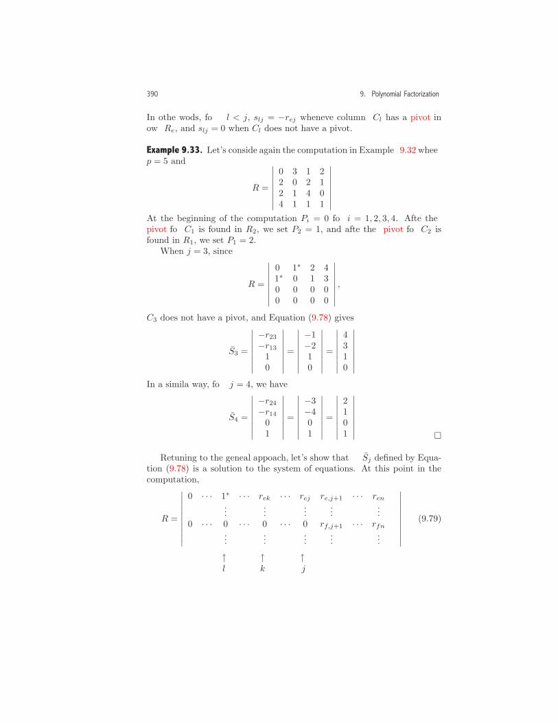
390 9. Polynomial Factorization
In other words, for l < j, slj = −rej whenever column Cl has a pivot inrow Re, and slj = 0 when Cl does not have a pivot.
Example 9.33. Let’s consider again the computation in Example 9.32 wherep = 5 and
R =
∣∣∣∣∣∣∣∣0 3 1 22 0 2 12 1 4 04 1 1 1
∣∣∣∣∣∣∣∣ .At the beginning of the computation Pi = 0 for i = 1, 2, 3, 4. After thepivot for C1 is found in R2, we set P2 = 1, and after the pivot for C2 isfound in R1, we set P1 = 2.
When j = 3, since
R =
∣∣∣∣∣∣∣∣0 1∗ 2 41∗ 0 1 30 0 0 00 0 0 0
∣∣∣∣∣∣∣∣ ,C3 does not have a pivot, and Equation (9.78) gives
S3 =
∣∣∣∣∣∣∣∣−r23−r1310
∣∣∣∣∣∣∣∣ =∣∣∣∣∣∣∣∣−1−210
∣∣∣∣∣∣∣∣ =∣∣∣∣∣∣∣∣4310
∣∣∣∣∣∣∣∣ .In a similar way, for j = 4, we have
S4 =
∣∣∣∣∣∣∣∣−r24−r1401
∣∣∣∣∣∣∣∣ =∣∣∣∣∣∣∣∣−3−401
∣∣∣∣∣∣∣∣ =∣∣∣∣∣∣∣∣2101
∣∣∣∣∣∣∣∣ . �
Returning to the general approach, let’s show that Sj defined by Equa-tion (9.78) is a solution to the system of equations. At this point in thecomputation,
R =
∣∣∣∣∣∣∣∣∣∣
0 · · · 1∗ · · · rek · · · rej re,j+1 · · · ren...
......
......
0 · · · 0 · · · 0 · · · 0 rf,j+1 · · · rfn...
......
......
∣∣∣∣∣∣∣∣∣∣(9.79)
↑ ↑ ↑l k j

9.3. Factorization in Zp[x] 391
where row Re is a typical row with a pivot and row Rf is a typical rowwithout a pivot. To show that Re · Sj = 0, suppose that in Equation (9.79)column l contains the pivot and column k is another typical column to theleft of Cj . From Equation (9.78), the vector Sj has the form
Sj =
∣∣∣∣∣∣∣∣∣∣∣∣∣∣∣∣∣∣
:−rej:0:10:0
∣∣∣∣∣∣∣∣∣∣∣∣∣∣∣∣∣∣
← l
← k
← j. (9.80)
Using the corresponding entries in Re and Sj , we have
Re · Sj = 1 · (−rej) + · · ·+ rek · 0 + rej · 1 + · · ·+re,j+1 · 0 + · · ·+ ren · 0
= 0.
In row Rf , which does not contain a pivot, all entries in positions ≤ j are 0.Indeed, entries in columns with pivots are 0, and entries in other columnsare 0 because Rf does not contain a pivot. Therefore,
Rf · Sj = 0
and Sj is a solution to the system of equations. In fact, Sj is a solution tothe system of equations at the end of the computation because all futurechanges in R occur in columns j + 1 to n, and the entries of Sj are 0 forall positions from j + 1 to n.
Using the above scheme, we obtain a set of solutions to Equation (9.66)
S = {Sj | Cj does not have a pivot} (9.81)
where the notation indicates a new Sj is formed whenever Cj does not havea pivot.
To show that S is a basis we must show that: (1) the solutions in S arelinearly independent, and (2) each solution to Equation (9.66) is a linearcombination of the solutions in S. The linear independence follows directlyfrom the definition for Sj and is left to the reader (Exercise 6).
To show (2), we show that for any solution y to Equation (9.66), wehave
y =∑j
Cj does nothave a pivot
yj Sj .

392 9. Polynomial Factorization
We verify this by showing that for each component yl of y,
yl =∑j
Cj does nothave a pivot
yj slj . (9.82)
To show this, first assume that Cl (the column associated with the variableyl) does not have a pivot. With this assumption, Equation (9.78) impliesthat
slj ={0, if l �= j ,1, if l = j,
and so Equation (9.82) follows.On the other hand, suppose that Cl has a pivot with Pe = l, and
consider the entries in row Re at the end of the computation. First, theelimination steps give rel = 1, and rej = 0 for all other columns Cj thathave pivots. We also have rej = 0 when j < l, where Cj does not have apivot because, if this were not so, Re would contain a pivot for one of thesecolumns Cj . Therefore, substituting y into the eth equation, we obtain
yl +∑j > l
Cj does nothave a pivot
yj rej = 0. (9.83)
However, since Cl has a pivot in Re, Equation (9.78) implies that
slj =
{−rej , if l < j,1, if l = j,0, if j < l,
(9.84)
and Equations (9.83) and (9.84) imply
yl =∑j > l
Cj does nothave a pivot
yj (−rej)
=∑j
Cj does nothave a pivot
yj slj .
The procedureAuxiliary basis that obtains a basis is given in Figures 9.5and 9.6. Since the procedure is used by the Berlekamp factor procedure,the basis is returned as a list S of polynomials rather than as a list ofvectors.

9.3. Factorization in Zp[x] 393
Procedure Auxiliary basis(x, n, p);Input
x : a symbol;n : a positive integer;p : a prime > 1;
Outputa list containing a basis of one or more auxiliary polynomials;
GlobalR : an n by n matrix with entries in Zp;
Local Variablesi, P, S, j, pivot found , a, k, f, l, s, e, c;
Begin1 for i := 1 to n do2 P [i] := 0;3 S := [ ];4 for j := 1 to n do5 i := 1;6 pivot found := false;7 while not pivot found and i ≤ n do8 if R[i, j] �= 0 and P [i] = 0 then9 pivot found := true10 else i := i + 1;11 if pivot found then12 P [i] := j;13 a := Multiplicative inverse p(R[i, j], p);14 for l := 1 to n do15 R[i, l] := Irem(a ∗R[i, l], p);16 for k := 1 to n do17 if k �= i then18 f := R[k, j];19 for l := 1 to n do20 R[k, l] := Irem(R[k, l] − f ∗R[i, l], p)
Continued in Figure 9.6.
Figure 9.5. An MPL procedure that finds a basis of auxiliary polynomials. (Im-plementation: Maple (txt), Mathematica (txt), MuPAD (txt).)
In lines 1–2, the variables P [i] (which correspond to Pi in the abovediscussion) are initialized to 0. In the j loop that begins at line 4, weexamine each column of the current matrix R to determine if it contains apivot (lines 5–10). If a pivot is found, we perform the elimination step inEquations (9.76) and (9.77) (lines 12–20). The procedureMultiplicative inverse pin line 13 is described in Exercise 11 on page 59.

394 9. Polynomial Factorization
21 elseif not pivot found then22 s := xj−1;23 for l := 1 to j − 1 do24 e := 0;25 i := 1;26 while e = 0 and i ≤ n do27 if l = P [i] then e := i28 else i := i + 1;29 if e > 0 then30 c := Irem(−R[e, j], p);
31 s := s + c ∗ xl−1;32 S := Join(S, [s]);33 Return(S)
End
Figure 9.6. Continuation of Figure 9.5.
If a pivot is not found, we construct a basis solution (lines 22–31). Al-though the basis polynomial is defined by the vector in Equation (9.78),the component slj corresponds to the coefficient of xl−1 in a basis polyno-mial (see Equations (9.51) and (9.58)). Based on the property that slj = 1when l = j, at line 22 we initialize the polynomial to xj−1. The loopstarting at line 23 determines the coefficients of smaller powers of x. Thestatements in lines 24–28 determine if a column Cl has a pivot row, and, ifone is found, the row of the pivot is represented by the integer e. If Cl hasa pivot, the coefficient of the polynomial is determined (in Zp) at line 31,while if a pivot is not found, the coefficient is 0, and so no action is taken.
The matrices that arise in Berlekamp’s algorithm always have zeroesin column C1. Therefore, when Auxiliary basis is applied to these matri-ces, the first basis polynomial is always the polynomial 1. The procedureFind factors described below makes use of this observation.
The Find factors Procedure. The procedure Find factors, that finds theirrreducible factors using the list S of basis polynomials, is shown in Fig-ure 9.7. The procedure is based on the relationships in the followingtheorem.
Theorem 9.34. Let u be a square-free, monic polynomial in Zp[x], and leth be an auxiliary polynomial that satisfies the remainder equations (9.42)on page 374.

9.3. Factorization in Zp[x] 395
1. If w is monic and w|u, then
w =p−1∏j=0
gcd(w, h− j). (9.85)
2. Suppose that w is monic with w|u, and let g = gcd(w, h − j) withdeg(g) > 0. Then,
gcd(g, h− i) ={g, i = j,1, i �= j, (9.86)
and for q = quot(w, g),
q =p−1∏i = 0i = j
gcd(q, h− i). (9.87)
The proofs of these properties are left to the reader (Exercise 8). �
The relationship in Equation (9.85) shows that the basic factor rela-tionship in Equation (9.46) also holds for divisors w of u even though his defined in terms of u. This means that we can obtain the irrreduciblefactors of u using operations of the form
gcd(w, bk(x)− j), (9.88)
where w is either u or some (reducible or irrreducible) divisor of u obtainedearlier in the computation. The relationships in Equations (9.86) and (9.87)are used below to justify the logic of the algorithm. We illustrate theapproach in the next example.
Example 9.35. Let p = 5, and consider the polynomial u = x6+x5+x+4.Three basis polynomials were obtained in Example 9.30 (page 380), and sou has three factors. Since b1 = 1, we do not obtain new factors with thisbasis polynomial. Using the second basis polynomial b2 = x4 + 4x3 + 4x2,we have
gcd(u, b2 − j) = 1, j = 0, 1. (9.89)
However,
g = gcd(u, b2 − 2) = x4 + 4x3 + 4x2 + 3
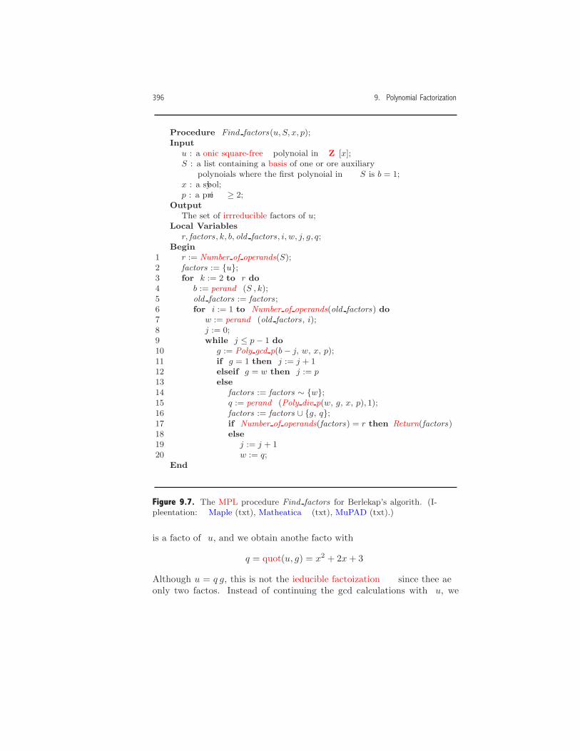
396 9. Polynomial Factorization
Procedure Find factors(u, S, x, p);Input
u : a monic square-free polynomial in Zp[x];S : a list containing a basis of one or more auxiliary
polynomials where the first polynomial in S is b = 1;x : a symbol;p : a prime ≥ 2;
OutputThe set of irrreducible factors of u;
Local Variablesr, factors , k, b, old factors , i, w, j, g, q;
Begin1 r := Number of operands(S);2 factors := {u};3 for k := 2 to r do4 b := Operand(S , k);5 old factors := factors ;6 for i := 1 to Number of operands(old factors) do7 w := Operand(old factors , i);8 j := 0;9 while j ≤ p− 1 do10 g := Poly gcd p(b− j, w, x, p);11 if g = 1 then j := j + 112 elseif g = w then j := p13 else14 factors := factors ∼ {w};15 q := Operand(Poly div p(w, g, x, p), 1);16 factors := factors ∪ {g, q};17 if Number of operands(factors) = r then Return(factors)18 else19 j := j + 120 w := q;
End
Figure 9.7. The MPL procedure Find factors for Berlekamp’s algorithm. (Im-plementation: Maple (txt), Mathematica (txt), MuPAD (txt).)
is a factor of u, and we obtain another factor with
q = quot(u, g) = x2 + 2x+ 3.
Although u = q g, this is not the irrreducible factorization since there areonly two factors. Instead of continuing the gcd calculations with u, we
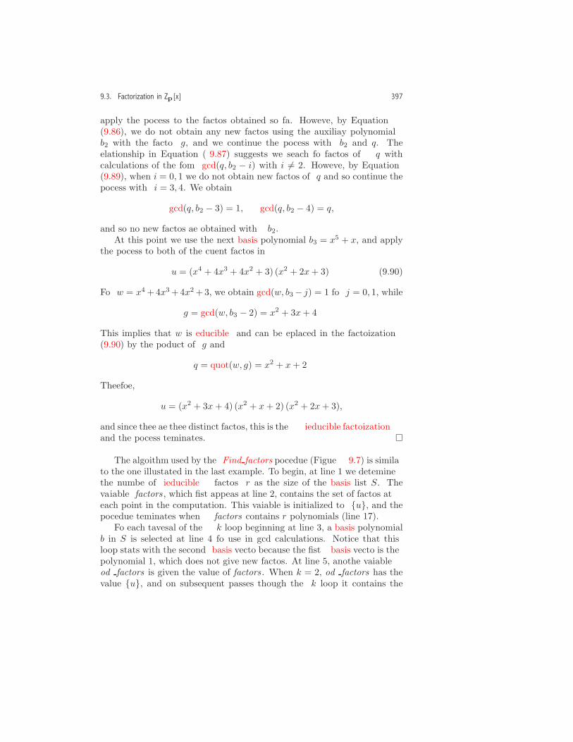
9.3. Factorization in Zp[x] 397
apply the process to the factors obtained so far. However, by Equation(9.86), we do not obtain any new factors using the auxiliary polynomialb2 with the factor g, and we continue the process with b2 and q. Therelationship in Equation (9.87) suggests we search for factors of q withcalculations of the form gcd(q, b2 − i) with i �= 2. However, by Equation(9.89), when i = 0, 1 we do not obtain new factors of q and so continue theprocess with i = 3, 4. We obtain
gcd(q, b2 − 3) = 1, gcd(q, b2 − 4) = q,
and so no new factors are obtained with b2.At this point we use the next basis polynomial b3 = x5 + x, and apply
the process to both of the current factors in
u = (x4 + 4x3 + 4x2 + 3) (x2 + 2x+ 3). (9.90)
For w = x4 +4x3+4x2+3, we obtain gcd(w, b3− j) = 1 for j = 0, 1, while
g = gcd(w, b3 − 2) = x2 + 3x+ 4.
This implies that w is reducible and can be replaced in the factorization(9.90) by the product of g and
q = quot(w, g) = x2 + x+ 2.
Therefore,
u = (x2 + 3x+ 4) (x2 + x+ 2) (x2 + 2x+ 3),
and since there are three distinct factors, this is the irrreducible factorizationand the process terminates. �
The algorithm used by the Find factors procedure (Figure 9.7) is similarto the one illustrated in the last example. To begin, at line 1 we determinethe number of irrreducible factors r as the size of the basis list S. Thevariable factors , which first appears at line 2, contains the set of factors ateach point in the computation. This variable is initialized to {u}, and theprocedure terminates when factors contains r polynomials (line 17).
For each traversal of the k loop beginning at line 3, a basis polynomialb in S is selected at line 4 for use in gcd calculations. Notice that thisloop starts with the second basis vector because the first basis vector is thepolynomial 1, which does not give new factors. At line 5, another variableold factors is given the value of factors . When k = 2, old factors has thevalue {u}, and on subsequent passes through the k loop it contains the

398 9. Polynomial Factorization
divisors obtained using the previous basis polynomials. We introduce thisnew variable because we reference each of the old factors at line 7, and thevalue of factors is changed whenever a new factor is found.
In the i loop beginning at line 6, we select an old factor w at line 7 andtry to find a new factor by applying the gcd operation in line 10 for variousvalues of j. Notice that when g = 1 (line 11), we have not found a newfactor, and so we increment j by 1 which continues the computation. Ifg = w, then Equation (9.85) implies that we will not find any new factorswith this w using the current basis function, and so we assign j to p, whichterminates the j loop.
If g is any other polynomial, then we have found a factor of w. At thispoint, we remove w from factors (line 14), add g and q = quot(w, g) tofactors (line 16), and check for termination at line 17. If this condition isnot satisfied, then by Equation (9.86), there is no reason to continue thegcd calculations with g and the current basis polynomial b because largervalues of j obtain a gcd of 1. In addition, Equation (9.87) implies thatany factors of q obtained with the current b are obtained with j valuesdifferent from the current j. However, none of the factors of the current qare obtained with earlier j values because they would have been obtainedearlier in the computation, and we would have a different q at this point.Therefore, we are justified in using larger values of j, and so we incrementj by 1 (line 10), assign the value of q to w (line 20), and continue lookingfor factors of the new w at line 9.
The process described in the previous paragraph is applied (using the iloop) to each of the old factors of u. If we don’t obtain all the factors withthe current basis polynomial, we continue the process with the next basispolynomial (lines 3, 4). Continuing in this fashion, we eventually obtainall factors of u.
Exercises
1. Give a procedure Square free factor p(u, x, p) that obtains the square-freefactorization of u using the recursive approach that is described beginningon page 373. Explain why the recursion terminates. (Exercise 9, page 125and Exercise 4, page 142 are useful in this problem.)
2. Let u be a monic polynomial in Zp[x] with deg(u) = n. Show that there are
(piquot(n,2)+1−p)/(p−1) trial factors of degree m with 1 ≤ m ≤ iquot(n, 2).
3. Let A and U be lists of r > 0 polynomials in Zp[x] that satisfy the condi-tions in the Chinese Remainder theorem (Theorem 4.41, page 140). Givea procedure Polynomial Chinese rem p(A,U, x, p).
4. (a) Show that h(x) = c (a constant polynomial in Zp) if and only ifa1 = a2 = · · · = ar = c.
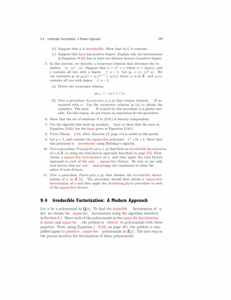
9.4. Irreducible Factorization: A Modern Approach 399
(b) Suppose that u is irrreducible. Show that h(x) is constant.
(c) Suppose that h(x) has positive degree. Explain why the factorizationin Equation (9.46) has at least two distinct factors of positive degree.
5. In this exercise, we describe a recurrence relation that determines the re-mainders rem(xp j , u). Suppose that u = xn + v where n = deg(u), andv contains all terms with a degree ≤ n − 1. Let yk = rem(xk, u). Wecan represent yk as yk(x) = ck x
n−1 + zk(x), where ck is in Zp and zk(x)contains all terms with degree ≤ n− 2.
(a) Derive the recurrence relation
yk+1 = −ck v + x zk.
(b) Give a procedure R matrix(u, x, n, p) that creates the matrix R as-sociated with u. Use the recurrence relation in (a) to obtain theremainders. The matrix R created by this procedure is a global vari-able. For this reason, do not return an expression from the procedure.
6. Show that the set of solutions S in (9.81) is linearly independent.
7. Use the algorithm that finds an auxiliary basis to show that the matrix inEquation (9.60) has the basis given in Equation (9.61).
8. Prove Theorem 9.34. Hint: Exercise 12, page 144 is useful in this problem.
9. Let p = 5, and consider the square-free polynomial x3 + 2x+ 4. Show thatthis polynomial is irrreducible using Berlekamp’s algorithm.
10. Give a procedure Trial factor p(u, x, p) that finds an irrreducible factorizationof u in Zp[x] using the trial-factors approach described on page 373. First,obtain a square-free factorization of u, and then apply the trial factorsapproach to each of the monic, square-free factors. Be sure to use onlytrial factors that are monic, and arrange the computation to minimize thenumber of trial divisors.
11. Give a procedure Factor p(u, x, p) that obtains the irrreducible factor-ization of u in Zp[x]. The procedure should first obtain a square-freefactorization of u and then apply the Berlekamp factor procedure to eachof the square-free factors.
9.4 Irreducible Factorization: A Modern Approach
Let u be a polynomial in Q[x]. To find the irrreducible factorization of u,first, we obtain the square-free factorization using the algorithm describedin Section 9.1. Since each of the polynomials in the square-free factorizationis monic and square-free, the problem is reduced to polynomials with theseproperties. Next, using Equation (9.24) on page 361, the problem is sim-plified again to primitive, square-free polynomials in Z[x]. The last step inthe process involves the factorization of these polynomials.

400 9. Polynomial Factorization
The algorithm described in this section obtains the irrreducible factorizationof a square-free, monic polynomial u in Z[x] by factoring a related poly-nomial in Zp[x] (for a suitable prime p) and then using the factors of thisnew polynomial to obtain the factors of u.Notation Conventions. In this section, we perform polynomial op-
erations in both Z[x] and Zm[x]. To distinguish the operations in the twocontexts, we adopt the following notation conventions.
1. For polynomial operations in Z[x], we use the ordinary infix symbolsfor addition (+) and multiplication (·).
2. For polynomial operations in Zm[x], we use the symbols ⊕m for ad-dition and ⊗m for multiplication that were introduced in Section 2.3.In this section, m is either a prime number p (in which case Zp is afield) or a positive integer power of a prime.
3. To simplify the notation, polynomials in both Z[x] and Zm[x] arerepresented using ordinary infix notation.
For example, u = x2 + 3 x+ 2 and v = x3 + 4 x+ 4 are polynomials inboth Z[x] and Z5[x]. We have, in Z[x],
u+ v = x3 + x2 + 7 x+ 6,
and, in Z5[x],u⊕5 v = x3 + x2 + 2 x+ 1.
Reduction to Monic Polynomials
The algorithm in this section applies to monic, square-free polynomials inZ[x]. Since the transformation in Equation (9.24) obtains a non- monic,primitive polynomial in Z[x], the first order of business is to restate thefactorization problem in terms of monic polynomials. Simply dividing apolynomial by its leading coefficient does not work, however, because somecoefficients of the new polynomial may not be integers. Instead, we proceedas follows. Let
u =n∑i=0
aixi
be a primitive polynomial in Z[x]. Our approach is to define a monicpolynomial v associated with u, factor v, and then use the factors of v toobtain the factors of u. Let
v = an−1n u(y/an) (9.91)
9.4. Irreducible Factorization: A Modern Approach 401
= an−1n
n∑i=0
ai(y/an)i (9.92)
=n−1∑i=0
an−1−in aiy
i + yn,
where v is a monic polynomial in Z[y]. Suppose that v has the irrreduciblefactorization
v = p1(y) · · · pr(y).One way to obtain a factorization for u is to invert the transformation inEquation (9.92):
u =(1/an−1
n
)v(an x) =
(1/an−1
n
)p1(an x) · · · pr(an x) (9.93)
although in this factorization, when an �= ±1, the leading constant is in Qbut not necessarily in Z. However, since
v(an x) = an−1n u
and since u is primitive, we have
cont(v(an x), x) = an−1n cont(u, x) = an−1
n .
Therefore, using Theorem 6.57, u has the factorization
u =(1/an−1
n
)v(an x)
=(1/an−1
n
)cont(v(an x), x) pp(v(an x), x)
= pp(v(an x), x)= pp(p1(anx), x) · · · pp(pr(anx), x). (9.94)
Example 9.36. Consider the primitive polynomial
u(x) = 8 x5 − 48 x4 + 90 x3 − 90 x2 + 117 x− 27.
Then,
v = 84 u(y/8) = y5 − 48 y4 + 720 y3 − 5760 y2 + 59904 y− 110592
which has the factorization
v = p1 p2 p3 = (y − 24)(y2 + 96
) (y2 − 24 y + 48
).
Inverting the transformation using Equation (9.93), we obtain
u = (1/4096) (8 x− 24)(64 x2 + 96
) (64 x2 − 192 x+ 48
).
However, using Equation (9.94), we have
u = pp(p1(8x), x) pp(p2(8x), x) pp(p3(8x), x)= (x− 3)
(2 x2 + 3
) (4 x2 − 12 x+ 3
). �

402 9. Polynomial Factorization
The Symmetric Representation for ZmLet m ≥ 2 be an integer. In Section 2.3 we considered the set
Zm = {0, 1, . . . ,m− 1} (9.95)
with the two binary operations
a⊕m b = irem(a+ b, m), a⊗m b = irem(a · b, m).
With these operations, Zm satisfies the field axioms F-1 through F-11, andsatisfies axiom F-12 if and only if m is prime (Theorem 2.41, page 53).The representation (9.95) is called the non-negative representation for Zmbecause all elements are non-negative integers.
Our algorithm factors a polynomial u in Z[x] by factoring a relatedpolynomial in Zm[x], and then using the factors in Zm[x] to obtain thefactors of u. Since u and its factors may have negative coefficients, we needanother representation for Zm that includes some negative integers. Thisalternate representation is defined as
Zm = {−iquot(m− 1, 2), . . . , 0, . . . , iquot(m, 2)}. (9.96)
For example,
Z5 = {−2,−1, 0, 1, 2}, Z6 = {−2,−1, 0, 1, 2, 3}.For m odd, this representation is symmetric about 0, while for m even,it is nearly symmetric with one more integer to the right of 0 than tothe left. For this reason, the representation (9.96) is called the symmetricrepresentation for Zm.
The connection between the two representations is defined as follows;each b in the non-negative representation is associated with the uniqueinteger in the symmetric representation given by
Sm(b) ={b, if 0 ≤ b ≤ iquot(m, 2),b−m, if iquot(m, 2) < b < m. (9.97)
For example, for m = 5, S5(3) = −2 and S5(4) = −1.For a and b in Zm in symmetric form, define the binary operations
a⊕m b = Sm(irem(a+ b, m)), a⊗m b = Sm(irem(a · b, m)).
For m = 5, the operations are given by the following tables.
⊕5 0 1 2 -2 -1
0 0 1 2 -2 -1
1 1 2 -2 -1 0
2 2 -2 -1 0 1
-2 -2 -1 0 1 2
-1 -1 0 1 2 -2
⊗5 0 1 2 -2 -1
0 0 0 0 0 0
1 0 1 2 -2 -1
2 0 2 -1 1 -2
-2 0 -2 1 -1 2
-1 0 -1 -2 2 1
9.4. Irreducible Factorization: A Modern Approach 403
The Projection from Z[x] to Zm[x]
The projection operator in the next definition defines the relationship be-tween Z[x] and Zm[x].
Definition 9.37. Let m ≥ 2 be an integer, and let u = an xn + · · ·+ a0 be
in Z[x].
1. For the non-negative representation of Zm, define
Tm(u) = irem(an, m)xn + · · ·+ irem(a0, m). (9.98)
2. For the symmetric representation of Zm, define
Tm(u) = Sm(irem(an, m))xn + · · ·+ Sm(irem(a0, m)). (9.99)
In either case, Tm(u) is called the projection of u in Zm[x].
Example 9.38. For u = x2 +5 x+8, using the non-negative representationof Z5, we have T5(u) = x2+3, while using the symmetric representation, wehave T5(u) = x2−2. Notice that there are infinitely many polynomials withthe projection x2 − 2. For example, using the symmetric representation,we also have T5(6 x2 + 10 x+ 13) = x2 − 2. �
To simplify our notation, we use the same operator Tm(u) for both thenon-negative and symmetric representations for Zm. In our mathematicaldiscussions, it will be clear from the context whether (9.98) or (9.99) isappropriate. In our procedures, however, we use the projection operatorsTnn(u, x, m) for the non-negative representation (9.98) and Ts(u, x, m)for the symmetric representation (9.99) (Exercise 2).
The projection operator satisfies the following properties.
Theorem 9.39. Let m ≥ 2 be an integer, and let v and w be polynomialsin Z[x]. Then, the projection operator satisfies the following properties.
1. deg(Tm(v)) ≤ deg(v) where the operator < applies when m|lc(v).2. Tm(v) = 0 if and only if m divides each coefficient of v.
3. For v in Zm[x], Tm(v) = v.
4. Tm(Tm(v)) = Tm(v).
5. Tm(v + w) = Tm(v)⊕mTm(w).6. Tm(v · w) = Tm(v)⊗mTm(w).

404 9. Polynomial Factorization
Proof: We prove the theorem using the non-negative, representation ofZm and leave the proof of the symmetric case to the reader (Exercise 3).
Parts (1), (2), and (3) follow directly from Definition 9.37, and Part (4)follows from Part (3).
To show (5), first for integers a and b, integer division gives
a = q1 m+ Tm(a), b = q2 m+ Tm(b). (9.100)
Therefore,
Tm(a+ b) = irem(a+ b, m)= irem(q1m+ Tm(a) + q2m+ Tm(b), m)= irem(Tm(a) + Tm(b), m)= Tm(a)⊕mTm(b). (9.101)
Part (5) follows for polynomials by applying this relationship to the corre-sponding coefficients of v and w.
To show (6), using (9.100), we obtain
Tm(a · b) = irem(q1q2 m2 + Tm(a)q2m+ Tm(b)q1m+ Tm(a)Tm(b),m
)= irem(Tm(a) · Tm(b), m)= Tm(a)⊗mTm(b). (9.102)
Part (6) follows for polynomials by applying Equations (9.101) and (9.102)to the coefficients of v · w. �
As a consequence of Theorem 9.39(5),(6), the polynomial operations⊕m and ⊗m can be obtained by performing the corresponding operationsin Z[x] (with expansion and automatic simplification) and then projectingthe results into Zm[x]. This point is illustrated in the next example.
Example 9.40. In Z7[x] (using the symmetric representation), we have
(2 x− 3)⊗7 (3 x− 1)⊗7
(x2 + 4 x− 1
)= T7(2 x− 3)⊗7 T7(3 x− 1)⊗7 T7
(x2 + 4 x− 1
)= T7
((2 x− 3) (3 x− 1) (x2 + 4 x− 1)
)= T7
(6 x4 + 13 x3 − 47 x2 + 23 x− 3
)= −x4 − x3 + 2 x2 + 2 x− 3. �
The next theorem gives some simple relationships between polynomialsin Z[x] and Zm[x] that are useful in our manipulations.
9.4. Irreducible Factorization: A Modern Approach 405
Theorem 9.41. Let u and v be polynomials in Zm[x]. Then, there arepolynomials h and k in Z[x] such that
u⊕mv = u+ v +mh,
u⊗mv = u · v +mk,
Tm(u) = u+mh,
where the operations on the right sides of the equations are performedin Z[x].
Proof: The theorem, which holds for either the non-negative or symmet-ric representations of Zm[x], follows directly from the definitions of thearithmetic operations in Zm (Exercise 8). �
Relationship of Factorization of u and Tm(u)Let’s return now to the factorization problem. Theorem 9.39(6) shows thata factorization of u in Z[x] is reflected in a factorization of Tm(u) in Zm[x].For example, in Z[x], we have
u = x2 + 11x+ 28 = (x+ 7)(x+ 4),
and in Z5[x], we have the symmetric representation
T5(u) = x2 + x− 2 = (x+ 2)⊗5(x− 1).
In some cases, however, the projection has more factors than u does. Forexample, in Z[x],
u = x3 + x2 + x+ 1 = (x+ 1)(x2 + 1),
while, in Z5[x],
T5(u) = (x+ 1)⊗5(x+ 2)⊗5(x− 2).
However, when m /| lc(u), Tm(u) cannot have fewer factors (of positivedegree) than u. Indeed, if
u = u1 · · ·urwhere each factor has positive degree, then Theorem 9.39(6) implies that
Tm(u) = Tm(u1)⊗m · · · ⊗mTm(ur).In addition, by Theorem 4.1 (page 112), m|/ lc(ui). and so Theorem 9.39(1)implies that each polynomial Tm(ui) has positive degree.

406 9. Polynomial Factorization
On the other hand, if m|lc(u), the projection may have fewer factors.For example, in Z[x],
u = 5 x2 + 11 x+ 2 = (5 x+ 1) (x+ 2)
while T5(u) = x+ 2.We summarize this discussion in the next theorem.
Theorem 9.42. Let u be a polynomial in Z[x] such that m /| lc(u).1. Suppose that the irrreducible factorization of u has r factors with pos-
itive degree and the irrreducible factorization of Tm(u) has s factorswith positive degree. Then, s ≥ r.
2. If Tm(u) is irrreducible in Zm[x], then u is irrreducible in Z[x].
Part (2) of the theorem is an important special case of Part (1).
Example 9.43. The converse of Theorem 9.42(2) is not true. For example,u = x2 + x+ 4 is irrreducible in Z[x], while
T5(u) = x2 + x− 1 = (x− 2)⊗5(x− 2)
in Z5[x]. In fact, T5(u) is not even square-free. �
Example 9.44. Let’s show that the polynomial
u = x3 + 6 x2 + 16 x+ 1
is irrreducible using Theorem 9.42(2). First, we try
T2(u) = x3 + 1 = (x+ 1)⊗2
(x2 + x+ 1
).
Since the projection is reducible, this gives no information about the re-ducibility of u. In a similar way,
T3(u) = x3 + x+ 1 =(x2 + x− 1
)⊗3 (x− 1)
andT5(u) = x3 + x2 + x+ 1 = (x+ 1)⊗5 (x+ 2)⊗5 (x− 2) ,
and so we still cannot arrive at a conclusion. However,
T7(u) = x3 − x2 + 2 x+ 1
is irrreducible in Z7[x], and therefore, u is irrreducible in Z[x]. �
9.4. Irreducible Factorization: A Modern Approach 407
The previous examples show that the irrreducible factorizations of uand Tm(u) can look quite different. The question is then: how can theirrreducible factorization of Tm(u) help obtain the factors of u?
Here is one approach. Let’s suppose that u has the irrreducible factor-ization
u = u1 · · ·ur (9.103)
in Z[x], and suppose thatm is large enough so that the coefficients of u andeach of its factors ui are in the symmetric representation of Zm[x]. Then,since Tm(u) = u and Tm(ui) = ui,
u = u1⊗m · · · ⊗muris a factorization of u in Zm[x]. However, if some of the ui are reducible inZm[x], this is not the irrreducible factorization for u in this setting.
On the other hand, if
u = v1⊗m · · · ⊗mvsis the irrreducible factorization of u in Zm[x], then each ui is either somevj or the product (in Zm[x]) of a number of vj . This suggests that each vjor the product of a number of vj is a possible factor of u in Z[x] and, bychecking all such polynomials, we can recover the factors ui in Equation(9.103). We illustrate this approach in the next example.
Example 9.45. Consider the polynomial
u = x4 + 5x3 + 6x2 + 5x+ 1
where u and each factor of u is in Z13[x]. Since 13 is prime, we factor thesquare-free polynomial u using Berlekamp’s algorithm which gives (in thesymmetric representation for Z13)
u = (x+ 4)⊗13(x+ 6)⊗13(x− 2)⊗13(x − 3).
However, none of these linear factors is a factor of u in Z[x].Let’s consider the trial factors obtained as the product of two of the
linear factors. For example, we try
v = (x+ 4)⊗13(x+ 6) = x2 − 3x− 2
but find, using polynomial division in Z[x], that v is not a factor. On theother hand,
v = (x + 4)⊗13(x− 3) = x2 + x+ 1
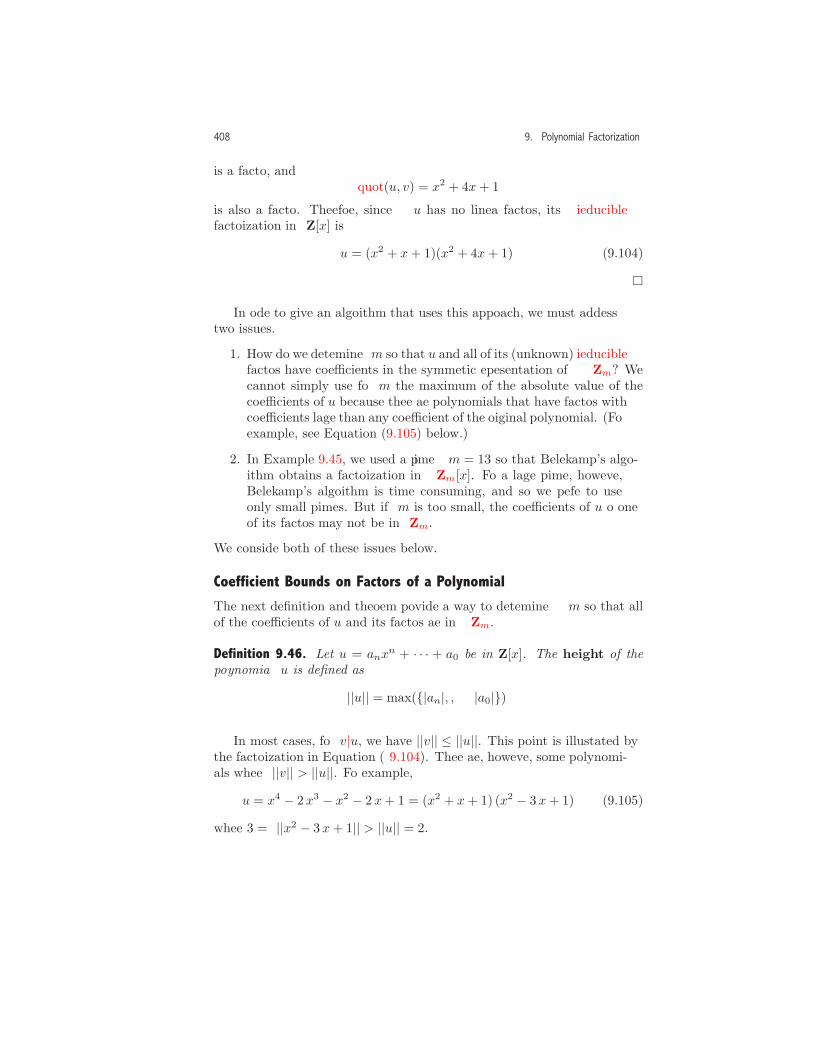
408 9. Polynomial Factorization
is a factor, andquot(u, v) = x2 + 4x+ 1
is also a factor. Therefore, since u has no linear factors, its irrreduciblefactorization in Z[x] is
u = (x2 + x+ 1)(x2 + 4x+ 1). (9.104)
�
In order to give an algorithm that uses this approach, we must addresstwo issues.
1. How do we determinem so that u and all of its (unknown) irrreduciblefactors have coefficients in the symmetric representation of Zm? Wecannot simply use for m the maximum of the absolute value of thecoefficients of u because there are polynomials that have factors withcoefficients larger than any coefficient of the original polynomial. (Forexample, see Equation (9.105) below.)
2. In Example 9.45, we used a prime m = 13 so that Berlekamp’s algo-rithm obtains a factorization in Zm[x]. For a large prime, however,Berlekamp’s algorithm is time consuming, and so we prefer to useonly small primes. But if m is too small, the coefficients of u or oneof its factors may not be in Zm.
We consider both of these issues below.
Coefficient Bounds on Factors of a Polynomial
The next definition and theorem provide a way to determine m so that allof the coefficients of u and its factors are in Zm.
Definition 9.46. Let u = anxn + · · · + a0 be in Z[x]. The height of the
polynomial u is defined as
||u|| = max({|an|, . . . , |a0|}).
In most cases, for v|u, we have ||v|| ≤ ||u||. This point is illustrated bythe factorization in Equation (9.104). There are, however, some polynomi-als where ||v|| > ||u||. For example,
u = x4 − 2 x3 − x2 − 2 x+ 1 = (x2 + x+ 1) (x2 − 3 x+ 1) (9.105)
where 3 = ||x2 − 3 x+ 1|| > ||u|| = 2.

9.4. Irreducible Factorization: A Modern Approach 409
The next theorem gives a bound on the coefficients of a factor of u.
Theorem 9.47. Let u and v be in Z[x] where v|u, and let n = deg(u).Then, ||v|| ≤ B where
B = 2n√n+ 1 ||u||. (9.106)
We do not prove this theorem, since the proof depends on some involvedmathematics that is well beyond the scope of this book. The general theorythat leads to this theorem is cited in the references at the end of thischapter. �
The upper bound B is usually considerably greater than the coefficientsof v. For example, for u in Equation (9.105),
B = 24√5 · 2 ≈ 71.55,
while the coefficients of both factors of u are actually bounded by 3. How-ever, B provides a way to obtain an m so that u and all of its irrreduciblefactors are in the symmetric representation Zm[x]. Since each b in Zm[x]satisfies |b| ≤ m/2 (see Equation (9.96)), we choose an integer m with
2B ≤ m. (9.107)
For example, for u in Equation (9.105),
m = 144 ≥ 2B ≈ 143.11.
Example 9.48. Consider the polynomial
u = x5 − 48x4 + 720x3 − 5760x2 + 59904x− 110592.
Then, ||u|| = 110592 and B = 25√6 110592. Therefore, for
m ≥ 26√6 · 110592,
all coefficients of u and its irrreducible factors are in Zm[x]. The actualvalue of m used in the factorization of u is determined in Example 9.57below. �
Hensel’s Lifting Theorem
We have described an approach that factors u in Z[x] by obtaining afactorization in Zm[x] for a suitably large positive integer m. AlthoughBerlekamp’s algorithm obtains the factorization when m is prime, it is not
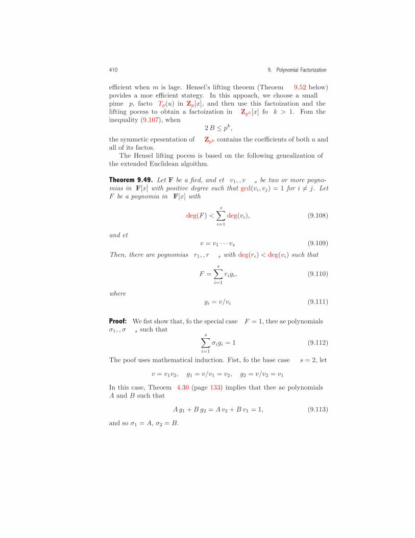
410 9. Polynomial Factorization
efficient when m is large. Hensel’s lifting theorem (Theorem 9.52 below)provides a more efficient strategy. In this approach, we choose a smallprime p, factor Tp(u) in Zp[x], and then use this factorization and thelifting process to obtain a factorization in Zpk [x] for k > 1. From theinequality (9.107), when
2B ≤ pk,
the symmetric representation of Zpk contains the coefficients of both u andall of its factors.
The Hensel lifting process is based on the following generalization ofthe extended Euclidean algorithm.
Theorem 9.49. Let F be a field, and let v1, . . . , vs be two or more polyno-mials in F[x] with positive degree such that gcd(vi, vj) = 1 for i �= j. LetF be a polynomial in F[x] with
deg(F ) <s∑i=1
deg(vi), (9.108)
and letv = v1 · · · vs. (9.109)
Then, there are polynomials r1, . . . , rs with deg(ri) < deg(vi) such that
F =s∑i=1
rigi, (9.110)
wheregi = v/vi. (9.111)
Proof: We first show that, for the special case F = 1, there are polynomialsσ1, . . . , σs such that
s∑i=1
σigi = 1. (9.112)
The proof uses mathematical induction. First, for the base case s = 2, let
v = v1v2, g1 = v/v1 = v2, g2 = v/v2 = v1.
In this case, Theorem 4.30 (page 133) implies that there are polynomialsA and B such that
Ag1 +B g2 = Av2 +B v1 = 1, (9.113)
and so σ1 = A, σ2 = B.

9.4. Irreducible Factorization: A Modern Approach 411
For the induction step, assume that Equation (9.112) is true for thes− 1 polynomials v1, . . . , vs−1. Define v and gi by Equations (9.109) and(9.111), and let
hi =v
vsvi, i = 1, . . . , s− 1. (9.114)
By the induction hypothesis, there are polynomials τ1, . . . , τs−1 such that
s−1∑i=1
τihi = 1. (9.115)
The polynomials gs = v/vs and vs are relatively prime, and so, by Theorem4.30, there are polynomials A and B such that
Avs + B gs = 1. (9.116)
In addition, from Equations (9.111), (9.114), and (9.115), we have
vs = vs
s−1∑i=1
τihi =s−1∑i=1
(τivsgsvi
)=s−1∑i=1
τigi. (9.117)
Therefore, using Equations (9.116) and (9.117), we obtain
1 = A
s−1∑i=1
τigi +B gs =s∑i=1
σigi (9.118)
where
σi ={Aτi, i = 1, . . . , s− 1,B, i = s. (9.119)
We now use Equation (9.112) to derive the representation (9.110) for ageneral polynomial F that satisfies the condition (9.108). From Equation(9.112), we have
s∑i=1
F σigi = F, (9.120)
and by polynomial division
F σi = qivi + ri (9.121)
whereqi = quot(F σi, vi), ri = rem(F σi, vi), (9.122)
and deg(ri) < deg(vi). Using Equations (9.111), (9.120), and (9.121), wehave
s∑i=1
rigi =s∑i=1
F σigi −s∑i=1
qivigi = F − vs∑i=1
qi. (9.123)
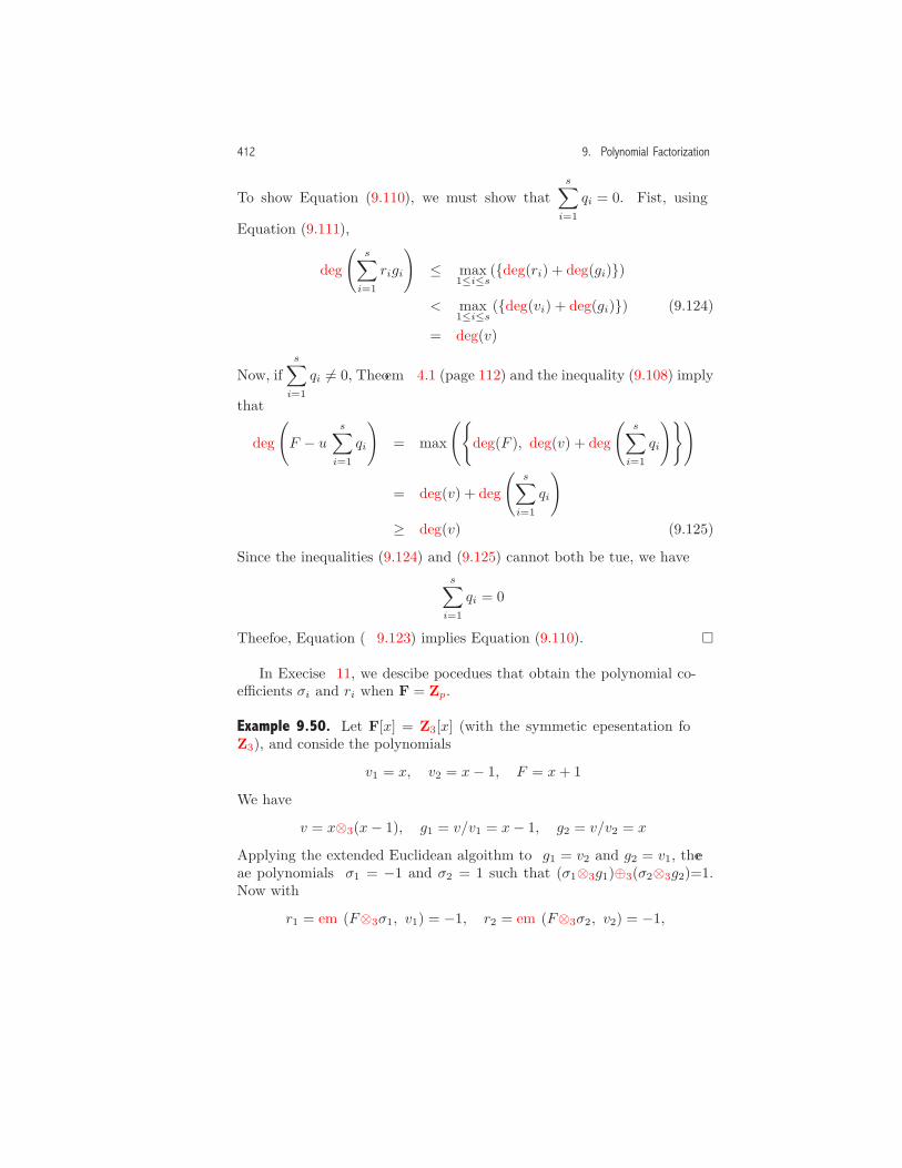
412 9. Polynomial Factorization
To show Equation (9.110), we must show thats∑i=1
qi = 0. First, using
Equation (9.111),
deg
(s∑i=1
rigi
)≤ max
1≤i≤s({deg(ri) + deg(gi)})
< max1≤i≤s
({deg(vi) + deg(gi)}) (9.124)
= deg(v).
Now, ifs∑i=1
qi �= 0, Theorem 4.1 (page 112) and the inequality (9.108) imply
that
deg
(F − u
s∑i=1
qi
)= max
({deg(F ), deg(v) + deg
(s∑i=1
qi
)})
= deg(v) + deg
(s∑i=1
qi
)
≥ deg(v). (9.125)
Since the inequalities (9.124) and (9.125) cannot both be true, we haves∑i=1
qi = 0.
Therefore, Equation (9.123) implies Equation (9.110). �
In Exercise 11, we describe procedures that obtain the polynomial co-efficients σi and ri when F = Zp.
Example 9.50. Let F[x] = Z3[x] (with the symmetric representation forZ3), and consider the polynomials
v1 = x, v2 = x− 1, F = x+ 1.
We have
v = x⊗3(x− 1), g1 = v/v1 = x− 1, g2 = v/v2 = x.
Applying the extended Euclidean algorithm to g1 = v2 and g2 = v1, thereare polynomials σ1 = −1 and σ2 = 1 such that (σ1⊗3g1)⊕3(σ2⊗3g2)=1.Now with
r1 = rem(F⊗3σ1, v1) = −1, r2 = rem(F⊗3σ2, v2) = −1,
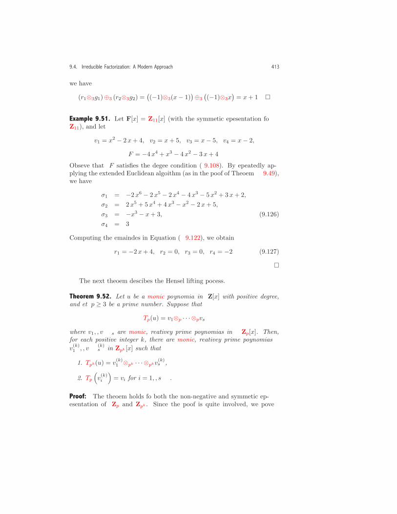
9.4. Irreducible Factorization: A Modern Approach 413
we have
(r1⊗3g1)⊕3 (r2⊗3g2) =((−1)⊗3(x− 1)
)⊕3
((−1)⊗3x
)= x+ 1. �
Example 9.51. Let F[x] = Z11[x] (with the symmetric representation forZ11), and let
v1 = x2 − 2 x+ 4, v2 = x+ 5, v3 = x− 5, v4 = x− 2,
F = −4 x4 + x3 − 4 x2 − 3 x+ 4.
Observe that F satisfies the degree condition (9.108). By repeatedly ap-plying the extended Euclidean algorithm (as in the proof of Theorem 9.49),we have
σ1 = −2 x6 − 2 x5 − 2 x4 − 4 x3 − 5 x2 + 3 x+ 2,σ2 = 2 x5 + 5 x4 + 4 x3 − x2 − 2 x+ 5,σ3 = −x3 − x+ 3, (9.126)σ4 = 3.
Computing the remainders in Equation (9.122), we obtain
r1 = −2 x+ 4, r2 = 0, r3 = 0, r4 = −2. (9.127)
�
The next theorem describes the Hensel lifting process.
Theorem 9.52. Let u be a monic polynomial in Z[x] with positive degree,and let p ≥ 3 be a prime number. Suppose that
Tp(u) = v1⊗p · · · ⊗pvswhere v1, . . . , vs are monic, relatively prime polynomials in Zp[x]. Then,for each positive integer k, there are monic, relatively prime polynomialsv(k)1 , . . . , v
(k)s in Zpk [x] such that
1. Tpk(u) = v(k)1 ⊗pk · · · ⊗pkv
(k)s ,
2. Tp
(v(k)i
)= vi for i = 1, . . . , s.
Proof: The theorem holds for both the non-negative and symmetric rep-resentation of Zp and Zpk . Since the proof is quite involved, we prove

414 9. Polynomial Factorization
the theorem for s = 2 using the symmetric representation. The proof,which uses mathematical induction, gives an algorithm for computing v
(k)1
and v(k)2 .
First, for the base case k = 1, v(1)1 = v1 and v
(1)2 = v2 satisfy properties
(1) and (2) of the theorem.Next, suppose that k ≥ 2, and let’s assume that we have found v
(k−1)1
and v(k−1)2 , and show how to lift one more step to find v
(k)1 and v
(k)2 . By the
induction hypothesis, property (1) of the theorem gives the factorizationin Zpk−1 [x]
Tpk−1(u) = v(k−1)1 ⊗pk−1v
(k−1)2 . (9.128)
However, the product v(k−1)1 v
(k−1)2 in Z[x] may not be a factorization of u,
and so we define the “error” in Z[x] between u and this factorization as
E = u− v(k−1)1 v
(k−1)2 . (9.129)
This error polynomial E is used to lift the factorization from Zpk−1 [x] toZpk [x].
First, let’s show that E satisfies the degree condition
deg(E) < deg(u). (9.130)
Since u is monic,
deg(u) = deg(Tpk−1(u)
)= deg
(v(k−1)1
)+ deg
(v(k−1)2
),
and since v(k−1)1 and v
(k−1)2 are also monic, the subtraction in Equation
(9.129) eliminates the highest degree monomial, which gives the inequality(9.130). In addition, since
deg(u) = deg (Tp(u)) = deg (v1) + deg (v2) ,
we havedeg(E) < deg (v1) + deg (v2) . (9.131)
By Equations (9.128) and (9.129),
Tpk−1(E) = 0,
and so Theorem 9.39(2) implies that pk−1 divides the coefficient of eachmonomial in E.
On the other hand, the projection Tpk(E) in Zpk [x] may not be 0,although the coefficient of each monomial in this projection has the form

9.4. Irreducible Factorization: A Modern Approach 415
r pk−1 where r is in Zp. To see why, since each coefficient of E has theform q pk−1, dividing q by p we obtain
q pk−1 = (a p+ s) pk−1 = a pk + s pk−1
where 0 ≤ s ≤ p− 1. From Equation (9.97), we have
Tpk
(q pk−1
)= Spk
(irem
(q pk−1, pk
))= Spk
(irem
(a pk + s pk−1, pk
))= Spk
(s pk−1
)=
{s pk−1, if 0 ≤ s pk−1 ≤ iquot
(pk, 2
),
s pk−1 − pk, if iquot(pk, 2
)< s pk−1 < pk
= r pk−1
where
r ={s, if 0 ≤ s ≤ iquot(p, 2),s− p, if iquot(p, 2) < s < p.
Therefore, the coefficient of each monomial in Tpk(E) has the form r pk−1
with r in Zp.Next, define
F = Tpk(E)/pk−1 (9.132)
where the above discussion shows that F is in Zp[x]. In addition, from theinequality (9.131), we have
deg(F ) < deg(v1) + deg(v2),
and so Theorem 9.49 implies that there are polynomials r1 and r2 in Zp[x]such that
(r2⊗pv1) ⊕p (r1⊗pv2) = F (9.133)
withdeg (r1) < deg (v1) , deg (r2) < deg (v2) . (9.134)
The polynomials r1 and r2 are used below to define the polynomials v(k)1
and v(k)2 .
However, before we do this, we need to mention a technical point. Sup-pose that b is in Zpk−1 and c is in Zp. Then, since the prime p ≥ 3 is odd,Equation (9.96) implies that
−pk−1 − 12
≤ b ≤ pk−1 − 12
, − p− 12≤ c ≤ p− 1
2.

416 9. Polynomial Factorization
Applying these inequalities to the expression b+ pk−1 c, we have
−pk−1 − 12
− pk−1
(p− 12
)≤ b + pk−1 c ≤ pk−1 − 1
2+ pk−1
(p− 12
),
and, therefore,
− pk − 12
≤ b+ pk−1 c ≤ pk − 12
(9.135)
which implies b+ pk−1 c is in Zpk .Define the polynomials at the next step k with
v(k)1 = v
(k−1)1 + pk−1r1, v
(k)2 = v
(k−1)2 + pk−1r2. (9.136)
We show that v(k)1 and v
(k)2 satisfy the properties the theorem. First, ap-
plying the inequality (9.135) to the coefficients of the monomials in v(k)1
and v(k)2 , it follows that both polynomials are in Zpk [x]. Next, since the
polynomials v(1)1 , v(k−1)
1 , v(1)2 , and v
(k−1)2 are all monic, property (2) of the
induction hypothesis implies that
deg(v(k−1)1
)= deg (v1) , deg
(v(k−1)2
)= deg (v2) . (9.137)
Therefore, the inequality (9.134) and Equations (9.136) and (9.137) implythat v(k)
1 and v(k)2 are also monic, and
deg(v(k)1
)= deg(v1), deg
(v(k)2
)= deg(v2).
To show that v(k)1 and v
(k)2 satisfy property (1), first observe, using
property (2) in the induction hypothesis and Theorem 9.41, there are poly-nomials M and N in Z[x] such that
v(k−1)1 = v1 + pM, v
(k−1)2 = v2 + pN. (9.138)
In addition, since, k ≥ 2, we have
2(k − 1) ≥ k,
and this inequality, Equations (9.136) and (9.138), and the properties ofthe projection operator (Theorem 9.39) imply that
v(k)1 ⊗pkv
(k)2 =
(v(k−1)1 + pk−1r1
)⊗pk
(v(k−1)2 + pk−1r2
)= Tpk
((v(k−1)1 + pk−1r1
) (v(k−1)2 + pk−1r2
))
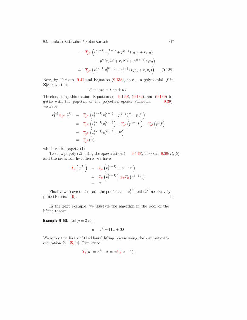
9.4. Irreducible Factorization: A Modern Approach 417
= Tpk
(v(k−1)1 v
(k−1)2 + pk−1 (r2v1 + r1v2)
+ pk (r2M + r1N) + p2(k−1)r1r2
)= Tpk
(v(k−1)1 v
(k−1)2 + pk−1 (r2v1 + r1v2)
). (9.139)
Now, by Theorem 9.41 and Equation (9.133), there is a polynomial f inZ[x] such that
F = r2v1 + r1v2 + p f.
Therefore, using this relation, Equations (9.129), (9.132), and (9.139) to-gether with the properties of the projection operator (Theorem 9.39),we have
v(k)1 ⊗pkv
(k)2 = Tpk
(v(k−1)1 v
(k−1)2 + pk−1(F − p f)
)= Tpk
(v(k−1)1 v
(k−1)2
)+ Tpk
(pk−1F
)− Tpk
(pkf
)= Tpk
(v(k−1)1 v
(k−1)2 + E
)= Tpk(u),
which verifies property (1).To show property (2), using the representation (9.136), Theorem 9.39(2),(5),
and the induction hypothesis, we have
Tp
(v(k)i
)= Tp
(v(k−1)i + pk−1ri
)= Tp
(v(k−1)i
)⊕pTp
(pk−1r1
)= vi.
Finally, we leave to the reader the proof that v(k)1 and v
(k)2 are relatively
prime (Exercise 9). �
In the next example, we illustrate the algorithm in the proof of thelifting theorem.
Example 9.53. Let p = 3 and
u = x2 + 11x+ 30.
We apply two levels of the Hensel lifting process using the symmetric rep-resentation for Z3[x]. First, since
T3(u) = x2 − x = x⊗3(x− 1),

418 9. Polynomial Factorization
we havev(1)1 = v1 = x, v
(1)2 = v2 = x− 1.
The preliminary calculations for this example were done in Example 9.50,where we obtained σ1 = −1 and σ2 = 1. We compute these polynomials atthe beginning of the process since they are used at each of the lifting steps.
To obtain v(2)1 and v
(2)2 , we have
E = u− v(1)1 v
(1)2 = 12 x+ 30
andF = T32(E)/3 = (3 x+ 3)/3 = x+ 1.
Again, from Example 9.50, we have r1 = −1 and r2 = −1. Therefore, inZ32 [x],
v(2)1 = T32(v(1)
1 + 3 r1) = x− 3, v(2)2 = T32(v(1)
2 + 3 r2) = x− 4.
To obtain v(3)1 and v
(3)2 , we have
E = u− v(2)1 v
(2)2 = 18 x+ 18
andF = T33(E)/32 = −x− 1.
At this step, by Equation (9.122),
r1 = rem(F⊗pσ1, v1) = −1, r2 = rem(F⊗pσ2, v2) = −1,
and, therefore,
v(3)1 = T33(v(2)
1 + 32 r1) = x+ 6, v(3)2 = T33(v(2)
2 + 32 r2) = x+ 5.
Since u = v(3)1 v
(3)2 is in Z[x], the lifting process terminates. (If we continue,
the next E = 0, and therefore v(4)1 = v
(3)1 and v
(4)2 = v
(3)2 .) �
Hensel Lifting Process. The Hensel lifting process is based on the follow-ing calculations. First, using Equations (9.113) and (9.119), we obtain asequence of polynomials σ1, . . . , σn in Zp[x] such that
(σ1⊗pg1)⊕p · · · ⊕p(σn⊗pgs) = 1, (9.140)
wherev = v1⊗p · · · ⊗pvs

9.4. Irreducible Factorization: A Modern Approach 419
(in unexpanded form) and gi = v/vi. The polynomials σi are computedat the beginning of the process because they are used at each lifting step.Next, let v
(1)i = v1, i = 1, . . . , s, and to obtain v
(j)i , . . . , v
(j)s (for 2 ≤ j ≤
k), let
E = u− v(j−1)1 · · · v(j−1)
s , (9.141)F = Tpj(E)/pj , (9.142)
where the algebraic operations (expansion and automatic simplification)are performed in Z[x]. Following this, we obtain the coefficient polynomialsri (for 1 ≤ i ≤ s), defined by Equation (9.122) with the operation (in Zp[x])
ri = rem(F⊗pσi, vi), i = 1, . . . , s. (9.143)
Finally, we obtain the new lifted factors with
v(j)i = Tpj
(v(j−1)i + pj−1ri
), i = 1, . . . , s, (9.144)
where the algebraic operation on the expression in parentheses is performedin Z[x].
Example 9.54. Consider the polynomial
u = x5 − 48 x4 + 720 x3 − 5760 x2 + 59904 x− 110592,
and let p = 11. By projecting u into Z11[x] and factoring the (square-free)projection using Berlekamp’s algorithm, we have (in the symmetric repre-sentation)
T11(u) = v = v1⊗11v2⊗11v3⊗11v4
=(x2 − 2 x+ 4
)⊗11 (x+ 5)⊗11 (x− 5) (9.145)⊗11 (x− 2)
= v(1)1 ⊗11v
(1)2 ⊗11v
(1)3 ⊗11v
(1)4 .
The preliminary calculations for this example were done in Example 9.51,where the σi are given in Equation (9.126). Then, from Equation (9.141)with j = 2,
E = u− (x2 − 2 x+ 4
)(x+ 5) (x− 5) (x− 2)
= −44 x4 + 737 x3 − 5852 x2 + 60104 x− 110792,
and therefore, by Equation (9.142),
F = T112(E)/11 = −4 x4 + x3 − 4 x2 − 3 x+ 4.

420 9. Polynomial Factorization
Again, from Example 9.51, the polynomials ri are given in Equation (9.127).Therefore, from Equation (9.144),
v(2)1 = x2 − 24 x+ 48, v
(2)2 = x+ 5, v
(2)3 = x− 5, v
(2)4 = x− 24.
In a similar way, for j = 3,
E = 121 x3 − 5808 x2 + 75504 x− 139392
andF = x3 − 4 x2 − 3 x+ 3.
From Equation (9.143), we have
r1 = 0, r2 = 1, r3 = −1, r4 = 0,
and from Equation (9.144), we have
v(3)1 = x2 − 24 x+ 48, v
(3)2 = x+ 126, v
(3)3 = x− 126, v
(3)4 = x− 24.
This example is continued in Examples 9.56 and 9.57 below. �
Choosing a Prime Number p. In order to apply the Hensel lifting process, theirrreducible factorization of Tp(u) in Zp[x] must have relatively prime (andtherefore distinct) factors. In other words, Tp(u) must be a square-freepolynomial. However, even though u is square-free, Tp(u) may not havethis property. (This happens in Example 9.43.) The next theorem shows,however, that it is always possible to find some prime p where Tp(u) issquare-free.
Theorem 9.55. Let p be a prime number, and let u be a square-free polyno-mial in Z[x] such that p/| lc(u). Then Tp(u) is not square-free for at mosta finite number of p.
Proof: Recall that Tp(u) is square-free if and only if
res(Tp(u), Tp(u)′) �= 0.
(See Theorem 7.9 (page 276) and Theorem 9.24 (page 372).) In addition,using Exercise 12,
res(Tp(u), Tp(u)′) = Tp(res(u, u′))
and since the integer res(u, u′) is divisible by at most a finite number ofprimes p, the theorem follows. �

9.4. Irreducible Factorization: A Modern Approach 421
Example 9.56. Consider the polynomial
u = x5 − 48 x4 + 720 x3 − 5760 x2 + 59904 x− 110592.
Then
res(u, u′) = −509012486930992988160000 = −2483105472.
Since 2, 3, 5, and 7 are divisors of the resultant, p = 11 is the first primefor which Tp(u) is square-free. �
Termination of the Hensel Lifting Process. There are two ways the Hensel lift-ing process can terminate. First, if at some point in the lifting process theerror polynomial E = 0, the most recently lifted factors v(j−1)
1 , . . . , v(j−1)s
are the true factors of u in Z[x]. This situation, which arises when u andTp(u) have the same number of irrreducible factors, occurs in Example9.53. On the other hand, if Tp(u) has more factors than u, the error poly-nomial E will never be 0. In this case, the lifting process continues untilwe are guaranteed that the symmetric representation of Zpk contains thecoefficients of u and all of its irrreducible factors. This situation arises inExample 9.57 below. Using the inequality (9.107), we choose this maximumlifting step to be the smallest integer k such that
2B ≤ pk, (9.146)
where B is defined in Equation (9.106). In this case, some of the liftedfactors may not be factors of u in Z[x]. This point is illustrated in the nextexample.
Example 9.57. In this example, we obtain the irrreducible factorization ofthe polynomial
u = x5 − 48 x4 + 720 x3 − 5760 x2 + 59904 x− 110592.
First, in Example 9.56 we determined that p = 11, and in Example 9.48 wedetermined that B = 25
√6 · 110592. Using the inequality (9.146), we have
k ≥ ln(2B)/ ln(p) ≈ 6.951,
and so k = 7. The factorization of T11(u) and the first two lifting steps aredescribed in Example 9.54. The lifting steps for j = 3, 4, 5, 6, and 7 aresimilar with
v(7)1 = x2−24 x+48, v
(7)2 = x−2868179, v
(7)3 = x+2868179, v
(7)4 = x−24.

422 9. Polynomial Factorization
This is an instance where there are more lifted factors than irrreduciblefactors of u. By polynomial division in Z[x], v(7)
1 and v(7)4 are irrreducible
factors of u, while v(7)2 and v
(7)3 are not. However, the polynomial v(7)
2 ⊗117
v(7)3 = x2 − 96 divides u, and so the irrreducible factorization in Z[x] is
u = (x2 − 24x+ 48) (x2 + 96) (x− 24). �
Procedures
The Irreducible factor Procedure. The procedure Irreducible factor , whichobtains the irrreducible factorization of a primitive, square-free polynomial,is shown in Figure 9.8. The global symbol y is a mathematical symbolintroduced at line 3. We have used a global symbol to avoid using a localvariable that would not be assigned before it was used (see page 3).
In lines 1–3, we obtain a monic polynomial V with the transformationin Equation (9.92). At line 4, the Find prime operator obtains a suitableprime number p that is guaranteed by Theorem 9.55 (Exercise 13). At line5, the Berlekamp factor operator (page 384) obtains the set of irrreduciblefactors of the projection of V in Zp[y]. Since Berlekamp factor is definedin terms of the non-negative representation of Zp[x], the operator Tnnprojects V into the non-negative representation (Exercise 2).
At line 6, if there is only one factor in S, the irrreducible polynomialu is returned. Otherwise, we find the value for k defined by the inequality(9.146) with the Find k operator (Exercise 17), and then, at line 9, findthe set of irrreducible factors with the Hensel lift operator (defined below).The Map operator in this statement transforms the factors in S to thesymmetric representation using the projection operator Ts described inExercise 2. Finally, in lines 10–15, we invert the monic transformationfrom line 3 (see Equation (9.94)).
The Hensel lift Procedure. A procedure that performs the Hensel liftingprocess is given in Figure 9.9. In lines 1–2, when k = 1 there is no liftingto be done. In this case, we recover the factors of u by applying theTrue factors operator (described below) to the set S.
The case k ≥ 2 is handled in lines 4–19. Since it is more convenient towork with a list of (distinct) factors than with a set, we obtain a list Vat line 4. (The operator Operand list obtains the list of operands of themain operator of an expression (see page 14).) In line 5, we obtain thecoefficient polynomials σi defined by Equation (9.140) using the operatorGen extend sigma p described in Exercise 11.
The actual lifting process is obtained in lines 6–18. At line 7, we forma product Vp of the factors in the list V . (The Construct operator, which

9.4. Irreducible Factorization: A Modern Approach 423
Procedure Irreducible factor(u , x);Input
u : a primitive, square-free polynomial in Z[x] with positive degree;x : a symbol;
OutputThe factored form of u;
Local Variablesn, l, V, p, S, k,W,M, i, w;
Global y;Begin
1 n := Degree gpe(u, x);2 l := Leading coefficient gpe(u, x);3 V := Algebraic expand(Substitute(ln−1 ∗ u, x = y/l));4 p := Find prime(V, y);5 S := Berlekamp factor(Tnn(V, y, p), y, p);6 if Number of operands(S) = 1 then Return(u)7 else8 k := Find k(V, y, p);9 W := Hensel lift(V, Map(Ts, S, y, p), y, p, k);10 W := Substitute(W, y = l ∗ x);11 M := 1;12 for i := 1 to Number of operands(W ) do13 w := Operand(W, i);14 M := M ∗Algebraic expand(w/Polynomial content(w, x, [ ], Z));15 Return(M)
End
Figure 9.8. An MPL procedure that obtains the irrreducible factorization ofa primitive, square-free polynomial in Z[x]. (Implementation: Maple (txt),Mathematica (txt), MuPAD (txt).)
creates the product, is described on page 9.) At line 8, we obtain the errorexpression E defined in Equation (9.129). In lines 9–10, if E = 0, we havefound the true factors in Z[x], which terminates the process, and so wereturn the set of factors. Otherwise, we perform the next lifting step bycomputing F (see Equation (9.142)) and the coefficient polynomials ri (seeEquation (9.143)) using the operator Gen extend R p described in Exercise11. In lines 14–18, we form the new list Vnew of lifted factors (see Equation(9.144)) and assign this to V in preparation for the next lifting step. If wecomplete the for loop that begins at line 6, V may have too many factors,which are combined at line 19 by the True factors operator.

424 9. Polynomial Factorization
Procedure Hensel lift(u, S, x, p, k);Input
u : a monic, square-free polynomial in Z[x] with positive degree;S : a set of relatively prime monic polynomials in Zp[x]
where Tp(u) is the product in Zp[x] of members of S.(The members of S use the symmetric representation of Zp);
x : a symbol;p : a prime ≥ 3;k : a positive integer;
Outputthe set of irrreducible factors of u;
Local Variablesi, j, R,Vp,Vnew , V, E, F, v lift, G;
Begin1 if k = 1 then2 Return(True factors(u, S, x, p, k))3 else4 V := Operand list(S);5 G := Gen extend sigma p(V, x, p);6 for j := 2 to k do7 Vp := Algebraic expand(Construct(” ∗ ”, V ));8 E := u− Vp;9 if E = 0 then10 Return(Construct(set, V ))11 else12 F := Algebraic expand Ts E, x, pj /pj−1 ;13 R := Gen extend R p(V,G, F, x, p);14 Vnew := [ ];15 for i := 1 to Number of operands(V ) do
16 v lift := Algebraic expand
Operand(V, i) + pj−1 ∗Operand(R, i) ;
17 Vnew := Join(Vnew , [v lift ])18 V := Vnew ;19 Return(True factors(u,Construct(set, V ), x, p, k))
End
Figure 9.9. An MPL procedure that performs the Hensel lifting process. (Imple-mentation: Maple (txt), Mathematica (txt), MuPAD (txt).)
The True factors Procedure. The last step in the algorithm uses the liftedfactors v
(k)1 , . . . , v
(k)s to determine the irrreducible factors of u. This step
is based on the observation that each factor of u is either one of the lifted

9.4. Irreducible Factorization: A Modern Approach 425
polynomials or the product (in Zpk [x]) of lifted polynomials. We improvethe efficiency of the algorithm by only testing trial factors that are theproduct of m lifted polynomials, where m ≤ s/2. Indeed, there is at mostone factor constructed with m > s/2, and this factor can be obtained bydividing all factors obtained with m < s/2 from u.
The True factors procedure shown in Figure 9.10 tests all trial factorsuntil the complete factorization is found. The input to the procedure in-cludes the polynomial u and a set l of lifted factors in Zpk [x], and theoutput is the set of irrreducible factors of u in Z[x].
In lines 1–2, we assign the values of u and l to the local variables U andL, which change in the course of the computation. At each point in thecomputation, U represents the divisor of u that remains to be factored, andL is the set of lifted polynomials that are used to factor U . The variablefactors initialized at line 3 contains the set of factors found so far, and thevariable m in line 4 represents the number of polynomials from L in a trialfactor. Since m is initialized to 1, the procedure first checks if each liftedpolynomial is a factor.
The operator Comb at line 6 obtains the set C of all m element subsetsof L (Exercise 15). The loop that begins at line 7 checks if a membert of C leads to a factor of U . In lines 9–10, we compute a trial factorT by expanding in Zpk [x] the product of the members of t. At line 11,we divide U by T , and, if the remainder (Operand(D, 2)) is 0, we haveobtained a factor of U which is added to factors (line 13). Since none ofthe polynomials in t can be used again in another factor, the members oft are removed from L (line 15), and any remaining m element sets in Cthat contain members of t are removed from C (line 16). (The operatorClean up is described in Exercise 14.) On the other hand, if the remainderOperand(D, 2) is not 0, we remove t from C (line 18) and return to thebeginning of the loop (line 7). Once all members of C have been eliminated,we increment m (line 19) and return to the beginning of the loop (line 5).
When the loop in lines 5–19 is done, there are two possibilities. If U = 1then all the factors of u have been found. On the other hand, if U �= 1,then this polynomial is also an irrreducible factor of u, and so it is addedto factors. In either case, the set of factors is returned at line 22.
We have given a basic version of the Berlekamp-Hensel polynomial fac-torization algorithm for polynomials in Q[x]. The polynomial factorizationproblem for single variable and multivariate polynomials with large coeffi-cients and many variables of high degree is a difficult computational prob-lem. There are, however, more sophisticated versions of the Berlekamp-Hensel algorithm and other algorithms that handle this problem more ef-ficiently than the algorithm given here. The references cited at the end ofthe chapter survey some of the recent developments for this problem.

426 9. Polynomial Factorization
Procedure True factors(u, l, x, p, k);Input
u : a monic, square-free polynomial in Z[x] with positive degree;l : the set of lifted factors in Zpk [x];x : a symbol;p : a prime number;k : a positive integer;
Outputthe set of irrreducible factors of u;
Local VariablesU,L, factors ,m,C, t, T,D;
Begin1 U := u;2 L := l;3 factors := ∅;4 m := 1;5 while m ≤ Number of operands(L)/2 do6 C := Comb(L, m);7 while C �= ∅ do8 t := Operand(C, 1);9 T := Construct(” ∗ ”, t);10 T := Ts(Algebraic expand(T ), x, pk);11 D := Polynomial division(U, T, x);12 if Operand(D, 2) = 0 then13 factors := factors ∪ {T};14 U := Operand(D, 1)15 L := L ∼ t;16 C := Clean up(C, t);17 else18 C := C ∼ {t};19 m := m + 1;20 if U �= 1 then21 factors := factors ∪ {U};22 Return(factors)
End
Figure 9.10. The MPL procedure that finds the irrreducible factors of u in Z[x]using the lifted polynomials. (Implementation: Maple (txt), Mathematica (txt),MuPAD (txt).)

9.4. Irreducible Factorization: A Modern Approach 427
Exercises1. Let b be in the non-negative representation of Zm. Show that Sm(b) is in
the symmetric representation of Zm. Hint: See Exercise 3, page 33.
2. Let u be a polynomial in Z[x].
(a) Give a procedure Tnn(u, x, m) that obtains the projection Tm(u)using the non-negative representation of Zm.
(b) Give a procedure Ts(u, x, m) that obtains the projection Tm(u)using the symmetric representation of Zm.
3. Prove Theorem 9.39 when Zm has the symmetric representation.
4. Let m and n be integers which are ≥ 2, and suppose that m|n. Show thatTm(Tn(u)) = Tm(u).
5. Suppose that u and v are in Z[x] where v|u.
(a) If deg(u) = 2, show that ||v|| ≤ ||u||.(b) Find an example with deg(u) = 3 where ||u|| < ||v||.(c) In Equation (9.105) we give an example where deg(u) = 4 and ||u|| <
||v||. Find another example.
6. Suppose that u and v are polynomials in Z[x] where v|u and deg(v) = 1.Show that ||v|| ≤ ||u||.
7. Suppose that u and v are polynomials in Z[x] where v|u and u, v andquot(u, v) have non-negative coefficients. Show that ||v|| ≤ ||u||.
8. Prove Theorem 9.41.
9. Show that the polynomials v(k)1 and v
(k)2 in the proof of Theorem 9.52 are
relatively prime.
10. (a) Factor x2 + 5x + 6 using the approach in this section.
(b) Show that x4 + 1 is irrreducible in Z[x] using the approach in thissection.
11. Let V be a list of two or more relatively prime, monic polynomials inZp[x], where p is a prime number and Zp is represented with the symmetricrepresentation.
(a) Give a procedure
Gen extend sigma p(V, x, p)
that returns the coefficient list [σ1, . . . , σs] defined by Equation (9.112),where σi is represented with the symmetric representation for Zp.
(b) Let S be the list obtained by Part (a), and let F be a polynomial inZp[x] that satisfies the inequality (9.108). Give a procedure
Gen extend R p(V, S, F, x, p)
that returns the list [r1, . . . , rs] defined by Equation (9.121), whereri is represented with the symmetric representation for Zp.

428 9. Polynomial Factorization
Note: This exercise uses operators for polynomial division (Exercise 9,page 125) and the extended Euclidean algorithm (Exercise 4, page 142)that must be modified to operate with the symmetric representation forZp[x].
12. Let p be a prime number and suppose that p /| lc(v) and p /| lc(w). Showthat Tm(res(v,w)) = res(Tm(v), Tm(w)), where the resultant on the rightis computed in Zp[x].
13. Let u be a square-free polynomial in Z[x]. Give a procedure
Find prime(u, x)
that returns a suitable prime number guaranteed by Theorem 9.55. Thisprocedure requires a list of primes. You can either provide a list of primesor use a CAS operator that generates prime numbers such as ithprime(n)in Maple, Prime[n] in Mathematica, and ithprime(n) in MuPAD (Im-plementation: Maple (mws), Mathematica (nb), MuPAD (mnb).)
14. Let C be a set whose members are also sets, and let t be another set. Givea procedure Clean up(C, t) that returns a new set which contains thosemembers s of C such that s ∩ t = ∅. For example, if
C = {{1, 2}, {1, 3}, {1, 4}, {1, 5}, {2, 3}, {2, 4}, {2, 5}, {3, 4}, {3, 5}, {4, 5}}
and t = {1, 2}, then Clean up(C, t) → {{3, 4}, {3, 5}, {4, 5}}.
15. Let S be a set of mathematical expressions and let k be an integer with 0 ≤k ≤ Number of operands(S). Give a procedure Comb(S, k) that returns theset of all k element subsets of S. For example, if S = {a, b, c, d}, then
Comb(S, 2) → {{a, b}, {a, c}, {a, d}, {b, c}, {b, d}, {c, d}}.
The procedure can be defined by the following recursive transformationrule sequence.
(a) If k = Number of operands(S), then Comb(S, k) → {S}.
(b) Comb(S, 0) → {∅}.
(c) Let x = Operand(S, 1), T = S ∼ {x}, and D = Comb(T, k − 1). ForD = {S1, . . . , Sn}, let E = {S1 ∪ {x}, . . . , Sn ∪ {x}}. Then
Comb(S, k) → Comb(T, k) ∪E.
16. The height of a polynomial is the maximum of the absolute values of itscoefficients. Let u be an algebraic expression. Give a procedure
Polynomial height(u, x)
that returns the height of a polynomial. If u is not a polynomial in x,return the global symbol Undefined.

9.4. Irreducible Factorization: A Modern Approach 429
17. Let u be a polynomial in Z[x], and let p be a prime number. Give aprocedure Find k(u, x, p) that finds the integer k defined by the inequality(9.146). (See Exercise 16 for the computation of ||u||.)
18. Modify the procedure Factor sv (see Exercise 8, page 370) that factorspolynomials in Q[x] so that operator Irreducible factor replaces Kronecker.
Further Reading
9.1 Square-Free Polynomials and Factorization. The algorithm in thissection is given in Musser [73]. Yun [106] describes a number of algorithms forsquare-free factorization of single variable and multivariable polynomials, includ-ing the algorithm in Exercise 11 on page 359. Other square-free factorizationalgorithms are given in Wang and Trager [97].
9.3 Factorization in Zp[x]. The approach here is similar to the approach inKnuth [55] and Akritas [2]. See Dean [31] and Mignotte [66] for a discussion ofirrreducible factorization in Zp[x]. Berlekamp’s algorithm is also described Dav-enport, Siret, and Tournier [29], Mignotte and Stefanescu [67], Geddes, Czapor,and Labahn [39], Yap [105], Winkler [101], and Zippel [108].
9.4 Irreducible Factorization in Q[x], A Modern Approach. The approach
here is similar to the approach in Knuth [55] and Akritas [2]. Modern polynomial
factorization algorithms are also described in Davenport, Siret, and Tournier [29],
Geddes, Czapor, and Labahn [39], Mignotte and Stefanescu [67], von zur Gathen
and Gerhard [96], Yap [105], Winkler [101] and Zippel [108]. Zippel [108] gives
a theory on bounds of coefficients of divisors of a polynomial. Theorem 9.47 is
based on Proposition 87 in this book. Coefficient bounds are also discussed in
Akritas [2], Cohen [22], and Mignotte [66].


Bibliography
[1] Williams W. Adams and Philippe Loustaunau. An Introduction toGrobner Bases. Graduate Studies in Mathematics, Volume 3. Amer-ican Mathematical Society, Providence, RI, 1994.
[2] Alkiviadis G. Akritas. Elements of Computer Algebra with Applica-tions. John Wiley & Sons, New York, 1989.
[3] Michael Artin. Algebra. Prentice Hall, Inc., Englewood Cliffs, NJ,1991.
[4] E. J. Barbeau. Polynomials. Springer-Verlag, New York, 1989.
[5] David Barton and Richard Zippel. Polynomial decomposition algo-rithms. Journal of Symbolic Computation, 1(1):159–168, 1985.
[6] Thomas Becker, Volker Weispfenning, and Heinz Kredel. Grobnerbases, A Computational Approach to Commutative Algebra. Springer-Verlag, New York, 1993.
[7] Laurent Bernardin. A review of symbolic solvers. SIGSAM Bulletin,30(1):9–20, March 1996.
[8] Laurent Bernardin. A review of symbolic solvers. In Michael J.Wester, editor, Computer Algebra Systems, A Practical Guide, pages101–120. John Wiley & Sons, Ltd., New York, 1999.
[9] A. S. Besicovitch. On the linear independence of fractional powers ofintegers. J. London Math. Soc., 15:3–6, 1940.
431
432 Bibliography
[10] Garrett Birkhoff and Saunders Mac Lane. A Survey of Modern Al-gebra. A K Peters, Ltd., Natick, MA, 1997.
[11] E. Bond, M. Auslander, S. Grisoff, R. Kenney, M. Myszewski, J. Sam-met, R. Tobey, and S. Zilles. Formac–An experimental formula ma-nipulation compiler. In Proc. 19th ACM National Conference, pagesK2.1–1–K2.1–11, August 1964.
[12] William E. Boyce and Richard C. DiPrima. Elementary DifferentialEquations. Sixth Edition. John Wiley & Sons, New York, 1997.
[13] Manuel Bronstein. Symbolic Integration I, Transcendental Functions.Springer-Verlag, New York, 1997.
[14] W. S. Brown. On Euclid’s algorithm and the computation of polyno-mial greatest common divisors. Journal of the Association for Com-puting Machinery, 18(4):478–504, October 1971.
[15] W. S. Brown. The subresultant prs algorithm. ACM Transactionson Math. Software, 4(3):237–249, September 1978.
[16] W. S. Brown and J. F. Traub. On Euclid’s algorithm and the theory ofsubresultants. Journal of the Association for Computing Machinery,18(4):505–514, October 1971.
[17] B. Buchberger, G. E. Collins, R. Loos, and R. Albrecht. Com-puter Algebra, Symbolic and Algebraic Computation. Second Edition.Springer-Verlag, New York, 1983.
[18] Bruno Buchberger. Grobner bases: An algorithmic method in poly-nomial ideal theory. In N. K. Bose, editor, Recent Trends in Mul-tidimensional Systems Theory, pages 184–232. D. Reidel PublishingCompany, Dordrecht, Holland, 1985.
[19] Ronald Calinger. Classics of Mathematics. Moore Publishing Com-pany Inc., Oak Park, IL, 1982.
[20] Shang-Ching Chou. Mechanical Geometry Theorem Proving. D. Rei-del Publishing Company, Boston, 1988.
[21] Barry A. Cipra. Do mathematicians still do math. Science, 244:769–770, May 19, 1989.
[22] Henri Cohen. A Course in Computational Algebraic Number Theory.Springer-Verlag, New York, 1993.

Bibliography 433
[23] J. S. Cohen, L. Haskins, and J. P. Marchand. Geometry of equilib-rium configurations in the ising model. Journal of Statistical Physics,31(3):671–678, June 1983.
[24] Joel S. Cohen. Computer Algebra and Symbolic Computation: Ele-mentary Algorithms. A K Peters, Natick, MA, 2002.
[25] George Collins. Subresultants and reduced polynomial remaindersequences. J. ACM, 14:128–142, January 1967.
[26] George Collins. The calculation of multivariate polynomial resul-tants. J.ACM, 18(4):515–532, October 1971.
[27] George Collins. Computer algebra of polynomials and rational func-tions. American Mathematical Monthly, 80(7):725–754, September1973.
[28] Thomas H. Cormen, Charles E. Leiserson, and Ronald L. Rivest.Introduction to Algorithms. McGraw-Hill, New York, 1989.
[29] J. H. Davenport, Y. Siret, and E. Tournier. Computer Algebra, Sys-tems and Algorithms for Algebraic Computation. Academic Press,New York, 1988.
[30] P. J. Davis and R. Hersh. The Mathematical Experience. Birkhauser,Boston, MA, 1981.
[31] Richard A. Dean. Classical Abstract Algebra. Harper and Row, NewYork, 1990.
[32] William R. Derrick and Stanley I. Grossman. Differential Equationswith Applications. Third Edition. West Publishing Company, St.Paul, MN, 1987.
[33] F. Dorey and G. Whaples. Prime and composite polynomials. Journalof Algebra, 28:88–101, 1974.
[34] H. T. Engstrom. Polynomial substitutions. Amer. J. of Mathematics,63:249–255, 1941.
[35] James F. Epperson. An Introduction to Numerical Methods and Anal-ysis. John Wiley & Sons, New York, 2002.
[36] R. J. Fateman. Macsyma’s general simplifier. philosophy and op-eration. In V.E. Lewis, editor, Proceedings of MACSYMA’s Users’Conference, Washington, D.C., June 20–22 1979, pages 563–582.MITLaboratory for Computer Science, Cambridge, MA, 1979.

434 Bibliography
[37] Richard J. Fateman. Symbolic mathematics system evaluators. InMichael J. Wester, editor, Computer Algebra Systems, A PracticalGuide, 255–284. John Wiley & Sons, Ltd., New York, 1999.
[38] Richard J. Gaylord, N. Kamin, Samuel, and Paul R. Wellin. AnIntroduction to Programming with Mathematica, Second Edition.Springer-Verlag, New York, 1996.
[39] K.O. Geddes, S.R. Czapor, and G. Labahn. Algorithms for ComputerAlgebra. Kluwer Academic Publishers, Boston, 1992.
[40] Jurgen Gerhard, Walter Oevel, Frank Postel, and Stefan Wehmeier.MuPAD Tutorial, English Edition. Springer-Verlag, New York, 2000.
[41] John W. Gray. Mastering Mathematica, Programming Methods andApplications. Second Edition. Academic Press, New York, 1997.
[42] J. Gutierrez and T. Recio. Advances on the simplification of sine-cosine equations. Journal of Symbolic Computation, 26(1):31–70,July 1998.
[43] G. H. Hardy and E. M. Wright. An Introduction To The Theory ofNumbers. Oxford at The Clarendon Press, London, 1960.
[44] K. M. Heal, M. L. Hansen, and K. M. Rickard. Maple 6 LearningGuide. Waterloo Maple Inc., Waterloo, ON, Canada, 2000.
[45] Andre Heck. Introduction to Maple. Second Edition. Springer-Verlag,New York, 1996.
[46] I. N. Herstein. Topics in Algebra. Second Edition. Xerox PublishingCompany, Lexington, MA, 1975.
[47] E. W. Hobson. Treatise on Plane and Advanced Trigonometry. Sev-enth Edition. Dover Publications, Inc., New York, 1957.
[48] Douglas R. Hofstadter. Godel, Escher, Bach: An Eternal GoldenBraid. Random House Inc., New York, 1980.
[49] David J. Jeffrey and Albert D. Rich. Simplifying square roots ofsquare roots by denesting. In Michael J. Wester, editor, ComputerAlgebra Systems, A Practical Guide, pages 61–72. JohnWiley & Sons,Ltd., New York, 1999.
[50] Richard D. Jenks and Robert S. Sutor. Axiom, The Scientific Com-putation System. Springer-Verlag, New York, 1992.

Bibliography 435
[51] N. Kajler, editor. Computer-Human Interaction in Symbolic Compu-tation. Springer-Verlag, New York, 1998.
[52] Israel Kleiner. Field theory, from equations to axiomatization. part i.American Mathematical Monthly, 106(7):677–684, August-September1999.
[53] Israel Kleiner. Field theory, from equations to axiomatization. part ii.American Mathematical Monthly, 106(9):859–863, November 1999.
[54] Morris Kline. Mathematics and The Search for Knowledge. OxfordUniversity Press, New York, 1985.
[55] D. Knuth. The Art of Computer Programming, volume 2. SecondEdition. Addison-Wesley, Reading, MA, 1981.
[56] Donald Knuth, Ronald Graham, and Oren Patashnik. ConcreteMathematics, A Foundation For Computer Science. Addison-Wesley,Reading, MA, 1989.
[57] K. Korsvold. An on-line algebraic simplify program. Technical report,Stanford University, 1965. Stanford University Artificial IntelligenceProject, Memorandum 37.
[58] J. S. Kowalik, editor. Coupling Symbolic and Numerical Computingin Expert Systems. Elsevier Science Publishers, New York, 1986.
[59] Dexter Kozen and Susan Landau. Polynomial decomposition algo-rithms. Journal of Symbolic Computation, 7:445–456, 1989.
[60] Susan Landau. Simplification of nested radicals. SIAM J. Comput.,21(1):85–110, February 1992.
[61] Ulrich Libbrecht. Chinese Mathematics in the Thirteenth Century.MIT Press, Cambridge, MA, 1973.
[62] R. Lidl and H. Niederreiter. Introduction to Finite Fields and theirApplications. Revised Edition. Cambridge University Press, NewYork, 1994.
[63] C. C. Lin and L. A. Segel. Mathematics Applied to DeterministicProblems in the Natural Sciences. Classics in Applied Mathematics1. Society for Industrial and Applied Mathematics, Philadelphia,1988.
[64] John D. Lipson. Elements of Algebra and Algebraic Computing. Ben-jamin/Cummings, Menlo Park, CA, 1981.

436 Bibliography
[65] Stephen B. Maurer and Anthony Ralston. Discrete AlgorithmicMathematics. A K Peters, Ltd., Natick, MA, 1998.
[66] Maurice Mignotte. Mathematics for Computer Algebra. Springer-Verlag, New York, 1991.
[67] Maurice Mignotte and Doru Stefanescu. Polynomials, An Algorith-mic Approach. Springer-Verlag, New York, 1999.
[68] Bhubaneswar Mishra. Algorithmic Algebra. Springer-Verlag, NewYork, 1993.
[69] M. B. Monagan, K. O. Geddes, K. M. Heal, G. Labahn, S. M.Vorkoetter, and J. McCarron. Maple 6 Programming Guide. Wa-terloo Maple Inc., Waterloo, ON, Canada, 2000.
[70] Joel Moses. Symbolic Integration. PhD thesis, MIT, September 1967.
[71] Joel Moses. Algebraic simplification: A guide for the perplexed.Communications of the ACM, 14(8):527–537, August 1971.
[72] George M. Murphy. Ordinary Differential Equations and Their So-lutions. D. Van Nostrand, New York, 1960.
[73] David Musser. Algorithms for Polynomial Factorization. PhD thesis,Department of Computer Science, University of Wisconsin, 1971.
[74] Paul J. Nahin. An Imaginary Tale, The Story of√−1. Princeton
University Press, Princeton, NJ, 1998.
[75] Jurg Nievergelt, J. Craig Farrar, and Edward M. Reingold. Com-puter Approaches to Mathematical Problems. Prentice-Hall, Engle-wood Cliffs, NJ, 1974.
[76] F. S. Nowlan. Objectives in the teaching college mathematics. Amer-ican Mathematical Monthly, 57(1):73–82, February 1950.
[77] R. Pavelle, M. Rothstein, and J. P. Fitch. Computer algebra. Scien-tific American, 245:136–152, 1981.
[78] Louis L. Pennisi. Elements of Complex Variables. Holt, Rinehart andWinston, New York, 1963.
[79] Charles Pinter. A Book of Abstract Algebra. Second Edition.McGraw-Hill, New York, 1990.

Bibliography 437
[80] Marcelo Polezzi. A geometrical method for finding an explicit formulafor the greatest common divisor. American Mathematical Monthly,104(5):445–446, May 1997.
[81] Frank Postel and Paul Zimmermann. Solving ordinary differentialequations. In Michael J. Wester, editor, Computer Algebra Systems,A Practical Guide, pages 191–209. John Wiley & Sons, Ltd., NewYork, 1999.
[82] T. W. Pratt. Programming Languages, Design and Implementation.Second Edition. Prentice Hall, Englewood Cliffs, NJ, 1984.
[83] Gerhard Rayna. Reduce, Software for Algebraic Computation.Springer-Verlag, New York, 1987.
[84] D. Richardson. Some undecidable problems involving elementaryfunctions of a real variable. Journal of Symbolic Logic, 33(4):511–520, December 1968.
[85] J. F. Ritt. Prime and composite polynomials. Trans. Am. Math.Soc., 23:51–66, 1922.
[86] P. Sconzo, A. LeSchack, and R. Tobey. Symbolic computation of fand g series by computer. The Astronomical Journal, 70(1329):269–271, May 1965.
[87] George F. Simmons. Differential Equations with Applications andHistorical Notes. Second Edition. McGraw-Hill, New York, 1991.
[88] George F. Simmons. Calculus with Analytic Geometry. Second Edi-tion. McGraw-Hill, New York, 1996.
[89] Barry Simon. Symbolic magic. In Michael J. Wester, editor, Com-puter Algebra Systems, A Practical Guide, pages 21–24. John Wiley& Sons, Ltd., New York, 1999.
[90] Barry Simon. Symbolic math powerhouses revisited. In Michael J.Wester, editor, Computer Algebra Systems, A Practical Guide. JohnWiley & Sons, Ltd., New York, 1999.
[91] Trevor J. Smedley. Fast methods for computation with algebraicnumbers. Research Report CS-90-12, Department of Computer Sci-ence, University of Waterloo, May 1990.
[92] Jerome Spanier and Keith B. Oldham. An Atlas of Functions. Hemi-sphere Publishing Corporation, New York, 1987.

438 Bibliography
[93] Frederick W. Stevenson. Exploring the Real Numbers. Prentice Hall,Upper Saddle River, NJ, 2000.
[94] David R. Stoutemyer. Crimes and misdemeanors in the com-puter algebra trade. Notices of the American Mathematical Society,38(7):778–785, September 1991.
[95] R. Tobey, R. Bobrow, and S. Zilles. Automatic simplification inFormac. In Proc. AFIPS 1965 Fall Joint Computer Conference, vol-ume 27, pages 37–52. Spartan Books, Washington, DC, November1965. Part 1.
[96] Joachim von zur Gathen and Jurgen Gerhard. Modern ComputerAlgebra. Cambridge University Press, New York, 1999.
[97] Paul Wang and Barry Trager. New algorithms for polynomial squarefree decomposition over the integers. SIAM Journal of Comp., 8:300–305, 1979.
[98] Mark Allen Weiss. Data Structures and Problem Solving Using C++.Second Edition. Addison-Wesley, Reading, MA, 2000.
[99] Clark Weissman. Lisp 1.5 Primer. Dickenson Publishing Company,Belmont, CA, 1967.
[100] Michael J. Wester. Computer Algebra Systems, A Practical Guide.John Wiley & Sons, Ltd., New York, 1999.
[101] F. Winkler. Polynomial Algorithms in Computer Algebra. Springer-Verlag, New York, 1996.
[102] Stephen Wolfram. The Mathematica Book. Fourth Edition. Cam-bridge University Press., New York, 1999.
[103] D. Wooldridge. An algebraic simplify program in Lisp. Technicalreport, Stanford University, December 1965. Artificial IntelligenceProject, Memo 11.
[104] W. A. Wulf, M. Shaw, P. Hilfinger, and L. Flon. Fundamental Struc-tures of Computer Science. Addison-Wesley, Reading, MA, 1981.
[105] Chee Keng Yap. Fundamental Problems of Algorithmic Algebra. Ox-ford University Press, New York, 2000.
[106] David Y. Y. Yun. On square-free decomposition algorithms. In R. D.Jenks, Proceedings of the 1976 ACM Symposium of Symbolic andAlgebraic Computation, pages 26–35. ACM, New York, 1976.

Bibliography 439
[107] David Y. Y. Yun and David R. Stoutemyer. Symbolic mathematicalcomputation. In J. Belzer, A.G. Holzman, and A. Kent, editors,Encyclopedia of Computer Science and Technology, volume 15, pages235–310. M. Dekker, New York, 1980.
[108] Richard Zippel. Effective Polynomial Computation. Kluwer Aca-demic Publishers, Boston, 1993.
[109] Daniel Zwillinger. Handbook of Differential Equations. AcademicPress, Boston, MA, 1989.

Index
A (algebraic numbers), 55Absolute value(u), 14Actual parameters
for a function, 3for a procedure, 3
Adjoin(L), 4Admissible factor
of a product, 82Admissible term
of a sum, 83Akritas, A., 14Alg monic(u, x, p, α), 163Alg coeff simp(u, x, p, α), 163Alg collect(u), 61Alg divide(u, v, p, α), 151Algebraic expressions, 6
simplified structure, 6Algebraic number field, 57Algebraic numbers, 55
denesting problem, 162explicit, 56explicit nesting depth, 60field property, 289implicit, 56independence of, 155
Algebraic expand(u), 14Alg extend(u, v, x, p, α), 164Alg gen simp(u, p, α), 164Alg mult inverse(v, p, α), 151Alg poly expansion
(u, v, x, t, p, α), 164
Alg polynomial division(u, v, x, p, α), 152
Alg quotient(u, v, x, p, α), 152
Alg rational simplify sv(u, x, p, α), 164
Alg remainder(u, v, x, p, α), 152
Alg square free factor(u, x, p, α), 359
ASAE (u), 90Associates(u, v, x), 207
Automatic simplification, 5
basic quotienttransformation, 76
basic associativetransformations, 69
basic differencetransformations, 75
basic distributivetransformation, 65
basic identitytransformations, 76
basic numericaltransformations, 78
basic powertransformations, 74
basic unarytransformations, 78
context of, 5
Automatically simplified
441

442 Index
algebraic expression(ASAE), 81
Automatic simplify(u), 92Auxiliary basis(x, n, p), 393
Base(u), 90base(u), 81Base rep(n, b), 35Basic algebraic expression
(BAE), 80Berlekamp’s algorithm
auxiliary polynomials, 374Berlekamp, E.R., 374Berlekamp factor(u, x, p), 384Buchberger, B., 14
C (complex numbers), 47CAIN (Computer Algebra Informa-
tion Network), 14CAS, 1Ceiling(u), 34Ceiling function, 34Chinese remainder problem
for F[x], 140for integers, 28
Chinese remainder(X,M), 34Chinese remainder 2
(m, n, r, s), 36Clean up(C, t), 428Coeff exp mv(u, v, n, L), 229Coefficient explosion
in Euclid’s algorithmin Q[x], 131
Coefficient exp(u, v, x, i), 126Coefficient gpe(u, x, j), 12cof(b, c), 203cof(v, u), 117Cofactor
in F[x], 117in K, 203
Comb(S, k), 428Common divisor
in F[x], 118in an integral domain, 203of two integers, 19
Compare(u, v), 90
Complete sub-expression, 10Complete poly decomp
(u, x), 198Computer algebra system (CAS), 1COMPUTER ALGEBRA,
Algorithms, Systemsand Applications, 14
Consistent side relations, 320computational test, 342
Const(u), 90const(u), 83Construct (f, L), 9cont(u, x), 240Czapor, S.R., 14
Davenport, J.H., 14Decision structures, 3
in CAS languages, 6deg(u, x), 12
properties of, 112Degree
of a GME, 12of a GPE, 12
Degree argument, 115Degree exp(u, v, x), 126Degree exp mv(u, v, L), 229Degree gpe(u, x), 12Denominator(u), 14Denominator fun(u), 43Derivative(u, x), 14Derivative fun(u, x), 108DiffOp, 39Division p(s, t, p), 60Divisor
in F[x], 117of an integer (b | a), 19
Divisors(n), 34
Elim poly(G,L), 346Equivalent monomials (≡), 213Equivalent polynomials
with respect to siderelations, 318
Euclid’s gcd algorithmfor integers, 22in F[x], 128

Index 443
Euclidean propertyof polynomial division
in F[x], 114of pseudo-division, 239
Evaluate difference(v, w), 43Evaluate power(u, n), 42Evaluate product(v, w), 43Evaluate quotient(u), 42Evaluate sum(v, w), 43Explicit algebraic number, 289Explicit algebraic number
(u), 60Exponent(u), 90exponent(u), 81Expression
function notation for infixoperators, 39
main operator, 6algebraic, 6non-algebraic, 8structure, 6tree, 6
Extended Euclidean algorithmfor integers, 24in F[x], 132
Extended Euclidean algorithm(u, v, x), 134
Ext Euclidean alg p(u, v, x, p), 142
FactOp, 39Factor p(u, x, p), 399Factor sv(u, x), 370Fermat’s little theorem, 54Fibonacci numbers
and remaindersequences, 35
Fieldaxioms, 44division or quotient
operation, 51, 59exponentiation or power opera-
tion, 51, 59finite, 52, 59subtraction or difference opera-
tion, 51
Find factors(u, S, x, p), 396Find integer factors(v, w, x), 369Find k(u, x, p), 429Find min deg(u, x), 198Find min deg(S, x), 199Find polynomial(α, x), 292Find prime(u, x), 428Find S sets(L), 369Find x u values(u, x, s), 369Find Z poly(u, x), 369First(L), 4Fitch, J.P., 14Floor(u), 34Floor function, 34Formal parameters
in MPL, 3of a function, 3
FracOp, 39Fraction
in standard form, 37Fraction (fraction), 7Free of (u, t), 10Fundamental Theorem of
Arithmetic, 27
Galois field, 164Galois theory, 56Gauss’s Theorem, 242Gaussian rational number
expression (GRNE), 61Gaussian rational numbers, 47
standard form, 61G basis(F,L), 337gcd(a, b), 20, 230gcd(u, v, x), 232gcd(u, v, x), 127Geddes, K.O., 14General monomial expression
(GME), 11coefficient part, 11variable part, 11
General polynomial expression(GPE), 11
degree of, 12Generalized coefficients, 11Generalized variables, 11
444 Index
Gen extend R p(U,S,w, x, p), 427Gen extend sigma p(V, x, p), 427Gerhard, J., 14GPE, 11Greatest common divisor
primitive algorithm in K[x], 247in F[x], 126of two integers, 20Euclid’s algorithm in F[x], 128Euclid’s algorithm in Z, 22in K[x], 232in K, 229subresultant algorithm
in K[x], 252Grobner basis, 324
Hensel lift(u, S, x, p, k), 424Hilbert Basis Theorem, 340
Ideal, 322, 340basis, 322principal, 323
Identifieras a mathematical symbol or vari-
able, 2as a programming variable, 2
Integer expression, 108Integer divisor(n), 34Integer expression(u), 108Integer lcm(a, b), 36Integers, 17
least common multiple, 36pairwise relatively
prime, 28prime, 27relatively prime, 19remainder sequence, 22representation in base b, 35
Integral domain, 48, 202associates, 203greatest common divisor, 229irreducible expression, 204relatively prime, 204unit, 203unit normal, 230
Integer ext euc alg(a, b), 26
Integer gcd(a, b), 23iquot(a, b), 18irem(a, b), 18Irreducible factor (u, x), 423Iteration structures, 3
in CAS languages, 6
Join(L), 4
Kind(u), 8Kronecker (u, x), 364Kronecker factors
(S sets, u, x), 365
Labahn, G., 14Lagrange polynomial(P, x), 369lc(u, x), 12
properties of, 112lcm(a, b), 36lcm(u, v, L), 328Leading monomial, 214Leading monomial ideal, 341Leading coefficient gpe
(u, x), 12Leading monomial(u, L), 215Least common multiple
of monomials, 328Lexicographical order
of monomials, 213Lexicographical order
(u, v, L), 228Lipson, J.D., 14Lists
empty list([ ]), 3notation, 3operations, 4properties, 3
lm(u, L), 214LMI(F ), 341Local variables
in MPL, 3
Map operatorin CAS languages, 11
Maple, 1, 65, 70, 72, 73, 75, 90, 117,262, 333, 428

Index 445
decision structures, 6
iteration structures, 6
list operations, 4map operator, 11
polynomial operators, 13
primitive structural operations, 9
set operations, 4structure based operators, 9
Map(F, u), 10
Map(G, u, y, . . . , z), 10
Mathematica, 1, 65, 70, 71, 73, 75,90, 117, 333, 428
decision structures, 6
iteration structures, 6list operations, 4
Map operator, 11
polynomial operators, 13
primitive structural operations, 9set operations, 4
structure based operators, 9
Mathematical expressions
Data objects, 3program statements, 3
Mathematical operators
procedures for, 3
Mathematical pseudo-language(MPL), 2
Max({n1, . . . , nr}), 14Max(S)
with respect to lexicographical or-der, 220
Mb poly div(u, v, L), 222
mbquot(u, v, L), 216
Mb quotient(u, v, L), 222mbrem(u, v, L), 216
Mb remaineder (u, v, L), 222
Merge products(p, q), 102
Merge products(p, q), 107Mignotte, M., 14
Minimal polynomial
of an algebraic number, 147
Mishra, B., 14
Monomial lcm, 334Monomial list(u,L), 228
MPL
general form of afunction, 3
general form of aprocedure, 5
assignment, 3decision structures, 3iteration structures, 3operators
logical, 2relational, 2
use of formal parameters, 3use of local variables, 3
MPLoperators
algebraic, 2Mult inv 23 (u), 59Multiple division, 300Multiple quotients, 300Multiple remainder, 300Multiple division(u,F ,L), 317Multiplicative inverse p
(t, p), 60MuPAD, 1, 65, 70, 75, 90, 117, 333,
428decision structures, 6iteration structures, 6map operator, 11polynomial operators, 13primitive structural operations, 9set operations, 4structure based operators, 9
MuPADlist operations, 445
Mv poly gcd rec(u, v, L,K), 249Mv poly gcd(u, v, L,K), 248
Nest depth(u), 60Number of digits(n), 34Number of operands(u), 8Numerator (u), 14Numerator fun(u), 43Numerical part frac(r), 176
Operand(u, i)., 9Operand list(u), 14Operator

446 Index
structure based, 10Operator evaluation
and automatic simplification of ar-guments, 6
Partial fraction(f, x), 173Partial fraction 1
(u, v1, v2, x), 170Partial fraction 2 (u, v, x), 171Partial fraction 3 (u, v, x), 173Pavelle, R., 14Poly Chinese rem(A,U, x), 145Poly decomp 2 (u, x, t), 192Poly div p(u, v, x, p), 125Poly gcd p(u, v, x, p), 142Polynomial
height, 428square-free factorization, 353irreducible factorization
in F[x], 138content, 239decomposition
algorithm, 188complete , 181equivalent, 184
derivative in F[x], 350irreducible, 118leading monomial, 214monic, 112multivariate
main and auxiliaryvariables, 202
primitive, 241primitive part, 242reduced with respect to F , 300reducible, 118remainder sequence, 246square-free, 350
Polynomial decomposition, 124Polynomial division
in F[x], 113monomial-based, 215recursive, 208
Polynomial expansionin F[x], 119in Q[x1, . . . , xp], 223
Polynomial operatorsusing polynomial
expansion, 123Polynomial remainder sequence
in F[x], 128Polynomial, composite, 179Polynomial content sr
(u, x,R,K), 261Polynomial content
(u, x,R,K), 260Polynomial height(u, x), 428Polynomial Chinese rem p
(A,U, x, p), 398Polynomial division
(u, v, x), 116Polynomial divisors(u, x), 125, 192Polynomial exp(u, v, x), 126Polynomial expansion
(u, v, x, t), 122Polynomial gcd(u, v, x), 130Polynomial gpe(u, v), 11Polynomial resultant
(u, v, x), 281Polynomial resultant mv
(u, v, L,K), 283Polynomials
Relatively primein F[x], 118
PowOp, 39pp(u, x), 242Primitive gcd algorithm
in K[x], 247Primitive operators
general polynomialexpressions, 11
simplified mathematicalexpressions, 8
ProdOp, 39Pseudo-division, 237Pseudo division(u, v, x), 240Pseudo quotient(u, v, x), 240Pseudo remainder(u, v, x), 240psquot(u, x), 238psrem(u, x), 238
Q(u, v), 228

Index 447
Q (rational numbers), 45quot(u, v, x), 113Quotient(u, v, x), 116QuotOp, 39
R (mathematical real numbers), 45Rational expressions
proper, 166standard form in Q(x), 144
Rational numberin standard form, 37
Rational number expression(RNE), 38
Rational simplification, 144, 258Rational integrate(f, x), 176Rationally simplified form, 257Rational red 1 (a, b, c, n, x), 175Rational red 2
(r, s, a, b, c, n, x), 175Rational red 3 (g , p, j , x), 176Rational red 4 (g , p, j , x), 176Rational simplify(u,L), 261Rational simplify sv(u, x), 145Rec poly div(u, v, L,K ), 211recquot(u, v, x), 208Rec quotient(u, v, L,K), 211recrem(u, v, x), 208Rec remainder(u, v, L,K), 211Reduction, 308Reduction(u, F, L), 316Reduction quotients, 308Reduction remainder, 308Reduction step, 306Reduction step quotient, 306Reduction step remainder, 306rem(u, v, x), 113Remainder(u, v, x), 116Remainder representation
for integers, 28Represent basis(u, F, L), 347Rest(L), 4Resultant
and polynomial divisionin F[x], 277
Euclidean algorithm for, 281properties of, 270
and pseudo-divisionin K[x], 282
definition, 268Subresultant algorithm, 284
res(u, x), 268Return(u), 14Ritt’s decomposition
theorem, 183R matrix (u, x, n, p), 384, 399Rothstein, M., 14
sci.math.symbolic discussion site, 14Sets, 2
operations, 4sign(u), 358SIGSAM (Special Interest Group on
Symbolic and Algebraic Manip-ulation), 14
Simplified structureof differences, 7of factorials, 8of fractions, 7, 8of products, 7of quotients, 7of sums, 7
Simplify difference(u), 106Simplify difference(u), 108Simplify factorial(u), 106, 108Simplify function(u), 108Simplify Gaussian(u), 61Simplify integer power
(v, n), 95, 107Simplify power(u), 107Simplify power rec(u), 107Simplify power(u), 94Simplify product(u), 107Simplify product(u), 98Simplify product rec(L), 99Simplify quotient(u), 106Simplify quotient(u), 107Simplify rational number
(u), 37Simplify RNE(u), 40Simplify RNE rec(u), 40Simplify side relations
(u, F, L), 343

448 Index
Simplify function(u), 106
Siret, Y., 14S poly(u, v, L), 334
Square-free polynomial, 350Square free factor p(u, x, p), 398
Square free factor(u, x), 356Square free factor Z (u, x), 360
Sr polynomial resultant(u, v, L,K), 286
Sr polynomial resultant rec(u, v, L,K), 287
Stefanescu, D., 14
Stoutemyer, D.R., 14Subresultant gcd algorithm
in K[x], 252Sub resultant gcd rec
(u, v, L,K), 255
Substitute(u, t = r), 10Substitution
with polynomialexpansion, 123
SumOp, 39Sylvester’s matrix, 267
Symbol manipulation system, 1SymbolicNet, 14
Term(u), 90term(u), 83
Tm(u), 403Tnn(u, x, m), 403, 427
Tournier, E., 14Transcendental number, 58
Transformation rulesGRNE (Gaussian rational
number expressions), 61G, 163
MPRD (Merge products(p, q)), 102
RNE (Rational NumberExpressions), 38
RS-IN , 257
RS, 144, 257SINTPOW
(Simplify integerpower(v, n)), 95
SPOW (Simplify power(u)), 94
SPRDREC(Simplifyproduct rec rec(L)), 99
SPRD (Simplify product(u)), 98
RS-IN, 144Tree-size of an expression, 229Tree size(u), 229Trial factor p(u, x, p), 399Trig ident(u), 229True factors(u, s, x, p, k), 426Ts(u, x, m), 403, 427
Unique factorization domain, 204
Variables(u), 12Variables 2 (u), 61von zur Gathen, J., 14
Wester, M., 14Winkler, F., 14Wolfram, S., 1
Yap, C.K., 14Yun, D.Y.Y., 14
Z (integers), 17Zero divisor
in an integral domain, 203Zero divisors
in F[x], 112in fields, 50in integers, 48
Zero equivalence problemfor polynomial side
relations, 321Zippel, R., 14Zp, 52Zp
multiplicative inversesusing Fermat’s littletheorem, 55

A K Peters, Ltd.
ISBN 1-56881-159-4
ì<(sl&q)=ibbfji< +^-Ä-U-Ä-U
Computer Algebra andSymbolic ComputationM a t h e m a t i c a l M e t h o d s
J O E L S . C O H E NComputer Algebra andSymbolic ComputationM a t h e m a t i c a l M e t h o d s
J O E L S . C O H E N
A KPETERS
Computer Algebra and Symbolic ComputationCohen
Math
em
atical Me
tho
ds
Mathematica™, Maple™, and similar software packages provideprograms that carry out sophisticated mathematical operations. Inthis book the author explores the mathematical methods that formthe basis for such programs, in particular the application of algorithmsto methods such as algebraic simplification, polynomial decomposition,polynomial greatest common divisor computation, and polynomialfactorization.
This text:
• is well-suited for self-study and can be used as the basis foran advanced undergraduate or beginning graduate course.
• maintains the style set by Elementary Algorithms• introduces advanced methods to treat complex operations.• presents implementations in such programs as Mathematica™,
Maple™, and MuPAD™.• includes a CD with the complete text, hyperlinks, and algorithms
as well as additional reference files.
For the student, Mathematical Methods is an essential companion toElementary Algorithms, illustrating applications of basic ideas. Forthe professional, Mathematical Methods is a look at new applicationsof familiar concepts.


![Optimization for Machine Learning - Approximation Theory ... · [Austel et al., 2017] propose MINLP model Find simplest symbolic mathematical expression ... objective Constrain the](https://img.pdfslide.us/doc/110x75/5ccc9b9188c993b2538c9da1/optimization-for-machine-learning-approximation-theory-austel-et-al.jpg)


![Optimization for Machine Learning - wiki.mcs.anl.gov · [Austel et al., 2017] propose MINLP model Find simplest symbolic mathematical expression ... objective Constrain the \grammar"](https://img.pdfslide.us/doc/110x75/5ccc9b9188c993b2538c9d99/optimization-for-machine-learning-wikimcsanlgov-austel-et-al-2017-propose.jpg)