Embed Size (px)
Citation preview
us Army Corps of Engineers© Engineer Research and Development Center
Computer-Aided Structural Engineering Project
User's Guide: Computer Program for Simulation of Construction Sequence for Stiff Wall Systems with Multiple Levels of Anchors (CMULTIANC) William P. Dawkins, Ralph W. Strom, Robert M. Ebeling August 2003
Approved for public release; distribution is unlimited.
L
Computer-Aided Structural ERDC/iTL SR-03-1 Engineering Project August 2003
User's Guide: Computer Program for Simulation of Construction Sequence for Stiff Wall Systems with IVIultiple Levels of Anchors (CMULTIANC) William P. Dawkins
5818 Benning Drive Houston, TX 77096
Ralph W. Strom
9474 S. E. Carnaby Way Portland, OR 97266
Robert M. Ebeling
Information Technology Laboratory U.S. Army Engineer Research and Development Center 3909 Halls Ferry Road Vicksburg, MS 39180-6199
Final report
Approved for public release; distribution is unlimited
Prepared for U.S. Army Corps of Engineers Washington, DC 20314-1000
Under Work Unit 31589
ABSTRACT: This report describes the PC-based computer program CMULTIANC, used to evaluate the effects of staged construction activities (i.e., excavation and tieback post-tensioning) on wall and soil behavior. The CMULTIANC simplified construction sequencing analysis is applicable to stiff walls with a single row or multiple rows of post-tensioned tieback anchors. Top-down construction is assumed in this analysis procedure.
The retaining wall system is modeled using beam on inelastic foundation methods with elastoplastic soil- pressure deformation curves (R-y curves) used to represent the soil behavior. The R-y curves are developed within the CMULTIANC program in accordance with the reference deflection method. The retaining wall is analyzed on a per-unit length run of wall basis. One-dimensional finite elements are used to model the retaining wall with closely spaced inelastic concentrated springs to represent soil-to-structure interactions on both sides of the wall. Discrete concentrated, elastoplastic springs are used to represent the anchors.
For each level of excavation (associated with a particular tieback installation) CMULTIANC performs three sequential analyses: (a) staged excavation analysis (to the excavation level needed for anchor installation) to capture soil loading effects, (b) R-y curve shifting to capture plastic soil movement effects, and (c) tieback installation analysis to capture tieback anchor prestressing effects. R-y curves are shifted to capture the plastic movement that takes place in the soils as the wall displaces toward the excavation for those conditions where actual wall computed displacements exceed active computed displacements. R-y curve shifting is necessary to properly capture soil reloading effects as tieback anchors are post- tensioned and the wall is pulled back into the retained soil.
DISCLAIMER: The contents of this report are not to be used for advertising, publication, or promotional purposes. Citation of trade names does not constitute an official endorsement or approval of the use of such commercial products. All product names and trademarks cited are the property of their respective owners. The findings of this report are not to be construed as an official Department of the Army position unless so designated by other authorized documents.
Contents
Conversion Factors, Non-SI to SI Units of Measurement vii
Preface viii
1—Background on Tieback Retaining Wall Systems 1
1.1 Design of Flexible Tieback Wall Systems...... 1 1.2 Design of Stiff Tieback Wall Systems 2
1.2.1 Identifying stiff wall systems 3 1.2.2 Tieback wall performance objectives 5 1.2.3 Progressive design of tieback wall systems 7
1.3 RIGID 1 Method 9 1.4 RIGID 2 Method ■ 10 1.5 WINKLER 1 Method 10 1.6 WINKLER 2 Method H 1.7 NLFEM Method 12 1.8 Factors Affecting Analysis Methods and Results 12
1.8.1 Overexcavation 12 1.8.2 Ground anchor preloading 13
1.9 Construction Long-Term, Construction Short-Term, and Postconstruction Conditions 13
1.10 Construction-Sequencing Analyses 14
2—Computer Program CMULTIANC 16
2.1 Introduction 16 2.2 Disclaimer 16 2.3 System Overview 16 2.4 Anchors 1^ 2.5 Excavation Elevations 17 2.6 Soil Profile 18
2.6.1 Unit weights 18 2.6.2 Strength properties 18
2.7 Water 18 2.8 Vertical Surcharge Loads 19 2.9 Limiting Soil and Water Pressures 19 2.10 Calculation Points 19 2.11 Active and Passive Pressures 20
2.11.1 Undrained (cohesive) soils 20 2.11.2 Drained (cohesionless) soils 20 2.11.3 Pressure coefficients 20
III
2.11.4 Profiles with interspersed undrained and drained layers 22 2.11.5 Pressures due to surcharge loads 22
2.12 Water Pressures 22 2.13 Nonlinear Soil and Anchor Springs 22 2.14 Displacements at Limiting Forces 24 2.15 Shifted Soil Spring Curves 25 2.16 Anchor Springs 25 2.17 Finite Element Model 28
2.17.1 Typical element 28 2.17.2 Typical node 29
2.18 External Supports 29 2.19 Method of Solution 29 2.20 Stability of Solution 30 2.21 Computer Program 30 2.22 Input Data Files 31 2.23 Output Data File ""'"^31 2.24 Graphics 32 2.25 Construction Sequence Simulation 32
2.25.1 Input data 32 2.25.2 Stage 1: Initial conditions 32 2.25.3 Stage 2: Solution for initial conditions 33 2.25.4 Stage 3: Shift of SSI curves ^."33 2.25.5 Stage 4: Solution w^ith shifted SSI curves 33 2.25.6 Stage 5: Top anchor installation 33 2.25.7 Stage 6: Excavation 33 2.25.8 Subsequent stages 33
2.26 Units and Sign Conventions 34
3—Example Solutions 35
3.1 Introduction 35 3.2 Soletanche Wall Z'"ZZZ"''Z" 35 3.3 Bonneville Type Wall 1'1...".'..."."46 3.4 CacoiloWall !.m.'.".".50
References 55
Appendix A: Guide for Data Input Al
A.l Introduction Al A. 1.1 Source of input Al A. 1.2 Data editing Al A.1.3 Input data file generation Al A. 1.4 Sections of input Al A.l.5 Predefined data file A2
A.2 Heading A3 A.3 Wall Segment Data A3 A.4 Anchor Data A3 A.5 Soil Profile Data A4 A.6 Initial Water Data A6 A.7 Right-Side Surface Surcharge Data A6 A.8 Excavation Data AlO A.9 Wall Bottom Conditions Al 1
IV
A.IO Termination All
Appendix B: Abbreviated Input Guide Bl
SF298
List of Figures
Figure 1-1. Definition of span length Z, 4
Figure 2-1. Schematic of wall/soil system 17
Figure 2-2. Log-spiral passive pressure coefficients (after Department of the Navy 1982) 21
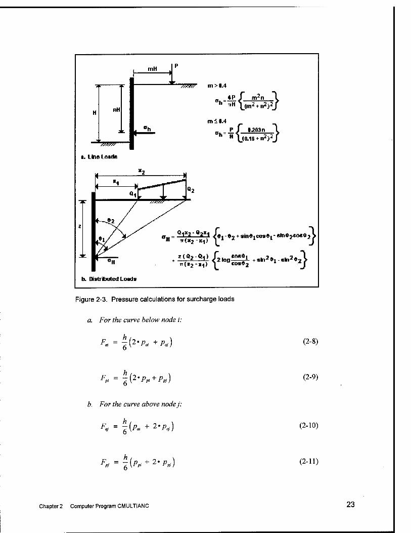
Figure 2-3. Pressure calculations for surcharge loads 23
Figure 2-4. Water pressures 24
Figure 2-5. Nonlinear soil springs 24
Figure 2-6. Concentrated soil springs 25
Figure 2-7. Shifted SSI soil springs 26
Figure 2-8. Nonlinear anchor spring 26
Figure 2-9. Finite element model 28
Figure 2-10. Typical element 28
Figure 2-11. Typical node 29
Figure 3-1. Soletanche wall 35
Figure 3-2. Input file for Soletanche wall 36
Figure 3-3. Echoprint of input data for Soletanche wall 37
Figure 3-4. Initial limit pressures for Soletanche wall 38
Figure 3-5. Initial SSI curves for Soletanche wall 39
Figure 3-6. Results for initial conditions for Soletanche wall 40
Figure 3-7. Shifted SSI curves for Soletanche wall 41
Figure 3 -8. Summary of results after anchor lock-off load for Soletanche wall 42
Figure 3-9. Summary of results for anchor spring replacing lock-off load for Soletanche wall 43
Figure 3-10. Limit pressures after excavation to elevation -30 for Soletanche wall 44
Figure 3-11. Left-side SSI curves after excavation to elevation -30 for Soletanche wall 44
Figure 3-12. Summary of results after excavation to elevation -30 for Soletanche wall 45
Figure 3-13. Maxima summary for Soletanche wall 46
Figure 3-14. Bonneville type wall simulation 46
Figure 3-15. Input file for Bonneville wall 47
Figure 3-16. Echoprint of input data for Bonneville wall 48
Figure 3-17. Maxima summary for Bonneville wall 50
Figure 3-18. Cacoilowall 50
Figure 3-19. Input file for Cacoilo wall 51
Figure 3-20. Echoprint of input data for Cacoilo wall 52
Figure 3-21. Initial water and soil limit pressures for initial conditions 54
Figure 3-22. Maxima summary for Cacoilo wall 55
List of Tables
Table 1-1.
Table 1-2.
Table 1-3.
Table 1-4.
Table 1-5.
Table 2-1.
Table 2-2.
Stiffness Categorization of Focus Wall Systems (Strom and Ebeling 2001) 4
General Stiffness Quantification for Focus Wall Systems (Strom and Ebeling 2001) 5
Design and Analysis Tools for Flexible Wall Systems (Ebeling et al. 2002) 7
Design and Analysis Tools for Stiff Wall Systems (Strom and Ebeling 2002) 8
Summary of R-y Curve Construction Methods (Strom and Ebeling 2001) 9
Reference Displacements 25
Units and Sign Conventions 34
VI
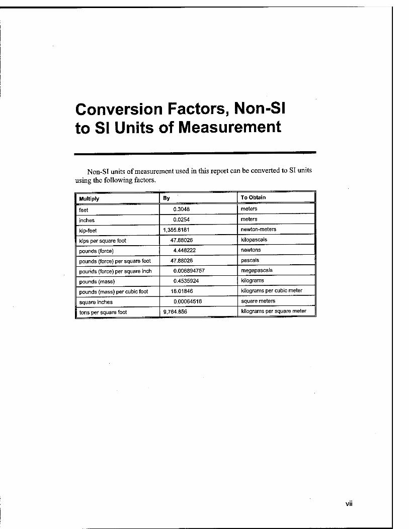
Conversion Factors, Non-SI to SI Units of Measurement
Non-SI units of measurement used in this report can be converted to SI units using the following factors.
Multiply By To Obtain
feet 0.3048 meters
Inches 0.0254 meters
kip-feet 1,355.8181 newton-meters
kips per square foot 47.88026 kilopascals
pounds (force) 4.448222 newtons
pounds (force) per square foot 47.88026 pascals
pourids (force) per square inch 0.006894757 megapascals
pounds (mass) 0.4535924 kilograms
pounds (mass) per cubic foot 16.01846 kilograms per cubic meter
square inches 0.00064516 square meters
tons per square foot 9,764.856 kilograms per square meter
VII
Preface
This report describes the software program CMULTIANC, newly developed to simulate the simplified construction sequence method of analysis of a stiff, tieback wall with multiple levels of prestressed anchors (assuming top-down construction). Funding for this research was provided by the Computer-Aided Structural Engineering Research Program sponsored by Headquarters, U.S. Army Corps of Engineers (HQUSACE), as part of the Infrastructure Technology Research and Development Program. Ms. Yazmin Seda-Sanabria, Geotechnical and Structures Laboratory (GSL), Vicksburg, MS, U.S. Army Engineer Research and Development Center (ERDC), was Program Manager. The study was conducted under Work Unit 31589, "Computer-Aided Structural Engineering (CASE)," for which Dr. Robert L. Hall, GSL, is Problem Area Leader and Mr. Chris Merrill, Chief, Computational Science and Engineering Branch, Information Technology Laboratory (ITL), ERDC, is Principal Investigator. The HQUSACE Technical Monitor is Ms. Anjana Chudgar, CECW-ED.
This report was prepared by Dr. William P. Dawkins, Houston, TX; Mr. Ralph W. Strom, Portland, OR; and Dr. Robert M. Ebeling, Engineering and Informatic Systems Division (EISD), ITL. Dr. Ebeling was the author of the scope of work for this research. The research was conducted under the direct supervision of Dr. Charles R. Welch, Chief, EISD; and Dr. Jeffery P. Holland, Director, ITL.
Commander and Executive Director of ERDC was COL John W. Morris III, EN. Director was Dr. James R. Houston.
VIII
1 Background on Tieback Retaining Wall Systems
This report describes the personal computer (PC) -based computer program CMULTIANC, used to simulate the simplified construction sequence method of analysis of a stiff tieback wall. Top-down construction is assumed in this analysis procedure.
The user's guide to CMULTIANC is given in Chapter 2. This chapter serves as an introduction to the categorization and analysis of "flexible" and "stiff tie- back retaining wall systems involving the use of prestressed anchors. The multi- anchored tieback earth retaining wall systems used by the U.S. Army Corps of Engineers are classified as either "flexible" or "rigid" according to Strom and Ebeling (2001, 2002) and Ebeling et al. (2002). The categorization of a tieback wall as being either flexible or rigid is used for convenience in determining the appropriate analysis and/or design procedure associated with a particular type (i.e., category) of wall.
1.1 Design of Flexible Tieback Wall Systems
The equivalent beam on rigid support method of analysis using apparent earth-pressure envelopes is most often the design method of choice, primarily because of its expediency in the practical design of tieback wall systems. This method provides the most reliable solution for flexible wall systems, i.e., soldier beam-lagging systems and sheet-pile wall systems, since for these types of systems a significant redistribution of earth pressures occurs behind the wall. Soil arching, stressing of ground anchors, construction-sequencing effects, and lagging flexibility all cause the earth pressures behind flexible walls to redistribute to, and concentrate at, anchor support locations (FHWA-RD-98-066). This redistribution effect in flexible wall systems cannot be captured by equivalent beam on rigid support methods or by beam on inelastic foundation analysis methods where the active and passive limit states are defined in terms of Rankine or Coulomb coefficients. Full-scale wall tests on flexible wall systems (FHWA-RD-98-066) indicated that the active earth pressure used to define the minimxmi load associated with the soil springs behind the wall had to be reduced by 50 percent to match measured behavior. Since the apparent earth-pressure diagrams used in equivalent beam on rigid support analyses were developed fi-om measured loads, and thus include the effects of soil arching, stressing of ground anchors, construction-sequencing effects, and lagging flexibility, they provide a
Chapter 1 Background on Tieback Retaining Wall Systems
better indication of the strength performance of flexible tieback wall systems. This is not the case for *ftj5^wall systems, however, and in fact the diagrams are applicable only to those flexible wall systems in which
• Overexcavation to facilitate ground anchor installation does not occur.
• Ground anchor preloading is compatible with active limit state conditions.
• The water table is below the base of the wall.
The design of flexible wall systems is illustrated in Ebeling et al. (2002).
1.2 Design of Stiff Tieback Wall Systems
Construction-sequencing analyses are important in the evaluation of stiff tieback wall systems, since for such systems the temporary construction stages are often more demanding than the final permanent loading condition (Kerr and Tamaro 1990). This may also be true for flexible wall systems where significant overexcavation occurs and for flexible wall systems subject to anchor prestress loads producing soil pressures in excess of active limit state conditions. The purpose of the example problems contained herein is to illustrate the use of construction-sequencing analysis for the design of stiff tieback wall systems. Although many types of construction-sequencing analyses have been used in the design of tieback wall systems, only three types of construction-sequencing analyses are demonstrated in the example problems. The three construction- sequencing analyses chosen for the example problems are ones considered to be the most promising for the design and evaluation of Corps tieback wall systems:
• Equivalent beam on rigid supports by classical methods (identified as the RIGID 2 method by Strom and Ebeling 2002).
• Beam on inelastic foundation methods using elastoplastic soil-pressure deformation curves (R-y curves) that account for plastic (nonrecoverable) movements (identified as the WINKLER 1 method by Strom and Ebeling 2002).
• Beam on inelastic foundation methods using elastoplastic soil-pressure deformation curves (R-y curves) for the resisting side only with classical soil pressures applied on the driving side (identified as the WINKLER 2 method by Strom and Ebeling 2002).
The results from these three construction-sequencing methods are compared in Strom and Ebeling (2002) with the results obtained fi-om the equivalent beam on rigid support method using apparent pressure loading (identified herein as the RIGID I method). Recall that apparent earth pressures are an envelope of maxi- mum past pressures encountered over all stages of excavation. The results are also compared with field measurements and finite element analyses in Strom and Ebeling (2002).
Chapter 1 Background on Tieback Retaining Wall Systems
1.2.1 Identifying stiff wall systems
Five focus wall systems were identified and described in detail in Strom and Ebeling (2001):
• Vertical sheet-pile system with wales and post-tensioned tieback anchors.
• Soldier beam system with wood or reinforced concrete lagging and post- tensioned tieback anchors. For the wood lagging system, a permanent concrete facing system is required.
• Secant cyUnder pile system with post-tensioned tieback anchors.
• Continuous reinforced concrete slurry wall system with post-tensioned tieback anchors.
• Discrete concrete slurry wall system (soldier beams with concrete lagging) with post-tensioned tieback anchors.
Deformations and wall movements in excavations are a function of soil strength and wall stiffness, with wall stiffness a function of structural rigidity El of the wall and the vertical spacing of anchors L. Soil stiffness correlates to soil strength; therefore, soil strength is often used in lieu of soil stiffness to charac- terize the influence of the soil on wall displacements. Steel sheet-pile and steel soldier beams with timber lagging systems are considered to be flexible tieback wall systems. Secant cyUnder pile, continuous concrete slurry wall, and discrete concrete slurry wall systems are considered to be stiff tieback wall systems. The effect of wall stiffness on wall displacements and earth pressures is described in Xanthakos (1991) and in FHWA-RD-81-150. In the FHWA report, it is indicated that Clough and Tsui (1974) showed, by finite element analyses, that wall and soil movements could be reduced by increasing wall rigidity and tieback stiffiiess. None of the reductions in movements were proportional to the increased stiffiiess, however. For example, an increase in wall rigidity of 32 times reduced the movements by a factor of 2. Likewise, an increase in the tieback stiffiiess by a factor of 10 caused a 50 percent reduction in movements.
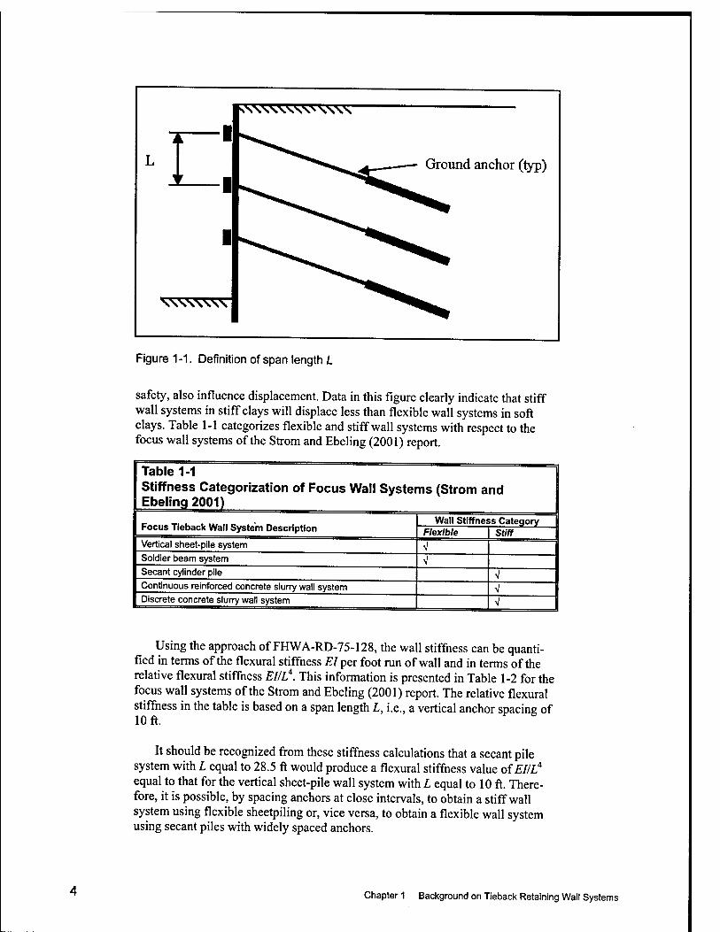
Other investigators have also studied the effect of support stiffness for clays (as reported in FHWA-RD-75-128). They defined system stiffness by EIIL'^, where El is the stiffiiess of the wall and L is the distance between supports (Figure 1-1). The measure of wall stiffness is defined as a variation on the inverse of Rowe's flexibility number for walls, and is thus expressed by EIIL^, where L is the vertical distance between two rows of anchors. Wall stiffness refers not only to the structural rigidity derived from the elastic modulus and the moment of inertia, but also to the vertical spacing of supports (in this case anchors). It is suggested by Figure 9-106 in FHWA-RD-75-128 that, for stiff clays with a stability number Y///5„ equal to or less than 3, a system stiffness EIIL^ of 10 or more would keep soil displacement equal to or less than 1 in.''^ However, other factors, such as prestress level, overexcavation, and factors of
' At this time, the authors of this report recommend that, when tieback wall system displacements are the quantity of interest (i.e., stringent displacement control design), they should be estimated by nonlinear finite element-soil structure interaction (NLFEM) analysis. ^ A table of factors for converting non-SI units of measurement to SI units is presented on page vii.
Chapter 1 Background on Tieback Retaining Wall Systems
s\vs\vs\
k^^V^V^S"sV^\\\
Ground anchor (typ)
Figure 1-1. Definition of span length L
safety, also influence displacement. Data in this figure clearly indicate that stiff wall systems in stiff clays will displace less than flexible wall systems in soft clays. Table 1-1 categorizes flexible and stiff wall systems with respect to the focus wall systems of the Strom and Ebeling (2001) report.
Table 1-1 Stimiess Categorization of Focus Wall Systems (Strom and Ebeling 2001)
Focus Tieback Wall System Description Wall Stiffness Cateqorv 1
Flexible stiff Vertical sheet-pile system V Soldier beam system V Secant cylinder pile V Continuous reinforced concrete sluny wall system V Discrete concrete slurry wall system V
Using the approach of FHWA-RD-75-128, the wall stiffness can be quanti- fied in terms of the flexural stiffness El per foot run of wall and in terms of the relative flexural stiffness EI/L'*. This information is presented in Table 1-2 for the focus wall systems of the Strom and Ebeling (2001) report. The relative flexural stiffness in the table is based on a span length L, i.e., a vertical anchor spacing of 10 ft.
It should be recognized from these stiffness calculations that a secant pile system with L equal to 28.5 ft would produce a flexural stiffness value of ^//Z," equal to that for the vertical sheet-pile wall system with L equal to 10 ft. There- fore, it is possible, by spacing anchors at close intervals, to obtain a stiff wall system using flexible sheetpiling or, vice versa, to obtain a flexible wall system using secant piles with widely spaced anchors.
Chapter 1 Background on Tieback Retaining Wall Systems
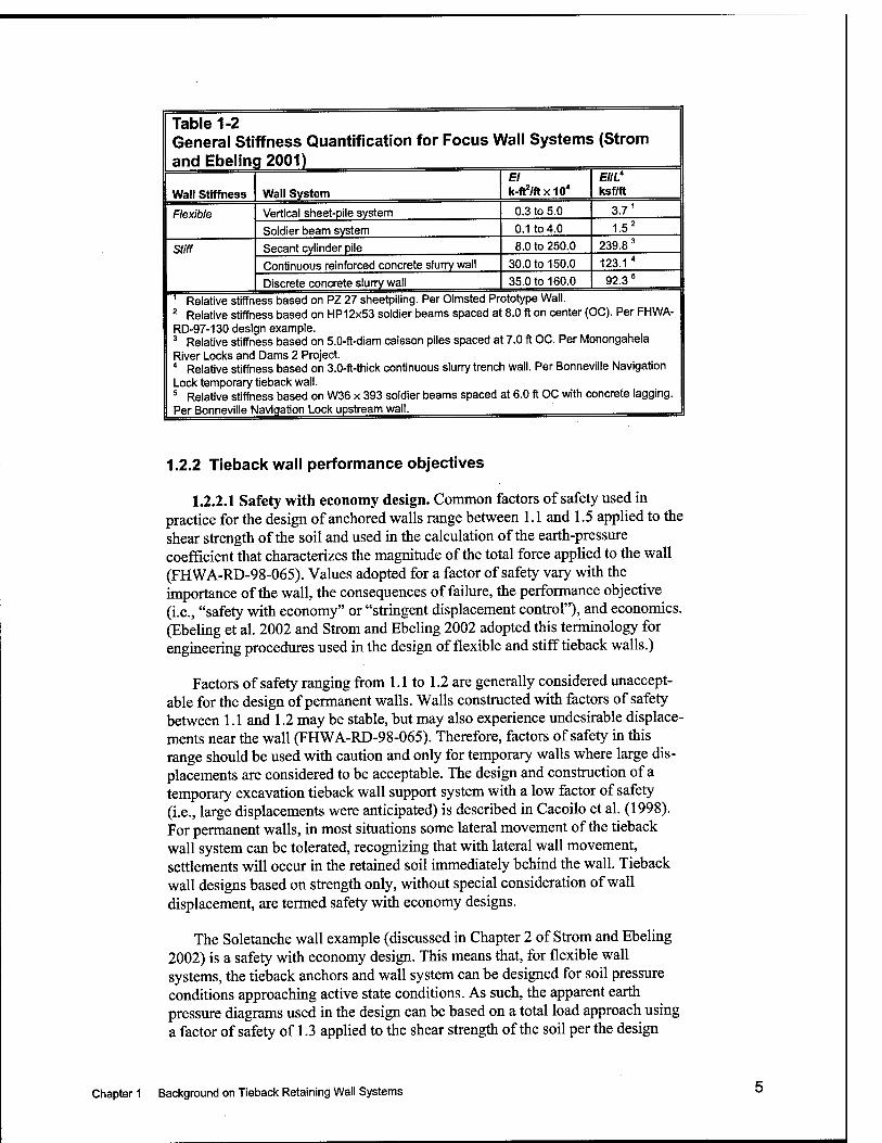
Table 1-2 General Stiffness Quantification for Focus Wall Systems (Strom and Ebelinq 2001)
Waif Stiffness Wall System El k-ft^/ftx10*
EIIL* ksf/fl
Flexible Vertical sheet-pile system 0.3 to 5.0 3.7^
Soldier beam system 0.1 to 4.0 1.5^
Stiff Secant cylinder pile 8.0 to 250.0 239.8 ^
Continuous reinforced concrete slun^ wall 30.0 to 150.0 123.1 *
Discrete concrete slun^ wall 35.0 to 160.0 92.3 =
' Relative stiffness based on PZ 27 sheetpiling. Per Olmsted Prototype Wall. ^ Relative stiffness based on HP12x53 soldier beams spaced at 8.0 ft on center (OC). Per FHWA- RD-97-130 design example. ^ Relative stiffness based on 5.0-ft-diam caisson piles spaced at 7.0 ft OC. Per Monongahela River Locl<s and Dams 2 Project. ■* Relative stiffness based on 3.0-ft-thick continuous slunv trencfi wall. Per Bonneville Navigation Locl< temporary tieback wall. ^ Relative stiffness based on W36 x 393 soldier beams spaced at 6.0 ft OC with concrete lagging. Per Bonneville Navigation Lock upstream wall.
1.2.2 Tieback wall performance objectives
1.2.2.1 Safety with economy design. Common factors of safety used in practice for the design of anchored walls range between 1.1 and 1.5 applied to the shear strength of the soil and used in the calculation of the earth-pressure coefiFicient that characterizes the magnitude of the total force applied to the wall (FHWA-RD-98-065). Values adopted for a factor of safety vary with the importance of the wall, the consequences of failure, the performance objective (i.e., "safety with economy" or "stringent displacement control"), and economics. (Ebeling et al. 2002 and Strom and Ebeling 2002 adopted this terminology for engineering procedures used in the design of flexible and stiff tieback walls.)
Factors of safety ranging from 1.1 to 1.2 are generally considered unaccept- able for the design of permanent walls. Walls constructed with factors of safety between 1.1 and 1.2 may be stable, but may also experience undesirable displace- ments near the wall (FHWA-RD-98-065). Therefore, factors of safety in this range should be used with caution and only for temporary walls where large dis- placements are considered to be acceptable. The design and construction of a temporary excavation tieback wall support system with a low factor of safety (i.e., large displacements were anticipated) is described in Cacoilo et al. (1998). For permanent walls, in most situations some lateral movement of the tieback wall system can be tolerated, recognizing that with lateral wall movement, settlements will occur in the retained soil immediately behind the wall. Tieback wall designs based on strength only, without special consideration of wall displacement, are termed safety with economy designs.
The Soletanche wall example (discussed in Chapter 2 of Strom and Ebeling 2002) is a safety with economy design. This means that, for flexible wall systems, the tieback anchors and wall system can be designed for soil pressure conditions approaching active state conditions. As such, the apparent earth pressure diagrams used in the design can be based on a total load approach using a factor of safety of 1.3 applied to the shear strength of the soil per the design
Chapter 1 Background on Tieback Retaining Wall Systems
recommendations of FHWA-RD-97-130. Trapezoidal earth pressure distributions are used for this type of analysis. For stiff wall systems, active earth pressures in the retained soil can often be assumed and used in a construction-sequencing analysis to size anchors and determine wall properties. Earth pressure distribution for this type of analysis would be in accordance with classical earth pressures theory, i.e., triangular with the absence of a water table.
The general practice for the safety with economy design is to keep anchor prestress loads to a minimum consistent with active, or near-active, soil pressure conditions (depending upon the value assigned to the factor of safety). This means the anchor size would be smaller, the anchor spacing larger, and the anchor prestress lower than those found in designs requiring "stringent displacement control."
1.2.2.2 "Stringent displacement control" design. A performance objective for a tieback wall can be to restrict wall and soil movements during excavation to a tolerable level so that structures adjacent to the excavation will not experience distress (as for the Bonneville temporary tieback wall example). According to FHWA-RD-81-150, the tolerable ground surface settlement may be less than 0.5 in. if a settlement-sensitive structure is founded on the same soil used for supporting the anchors. Tieback wall designs that are required to meet specified displacement control performance objectives are termed stringent displacement control designs. Selection of the appropriate design pressure diagram for deter- mining anchor prestress loading depends on the level of wall and soil movement that can be tolerated. Walls built with factors of safety between 1.3 and 1.5 applied to the shear strength of the soil may result in smaller displacements if stiff wall components are used (FHWA-RD-98-065).
To minimize the outward movement, the design would proceed using soil pressures at a magnitude approaching at-rest pressure conditions (i.e., a factor of safety of 1.5 applied to the shear strength of the soil). It should be recognized that even though the use of a factor of safety equal to 1.5 is consistent with an at-rest (i.e., zero soil-displacement condition) earth pressure coefficient (as shown in Figure 3-6 of Engineer Manual 1110-2-2502 (Headquarters, U.S. Army Corps of Engineers 1989)), several types of lateral wall movement could still occur. These include cantilever movements associated with installation of the first anchor; elastic elongation of the tendon anchor associated with a load increase; anchor yielding, creep, and load redistribution in the anchor bond zone; and mass move- ments behind the ground anchors (FHWA-SA-99-015). It also should be recog- nized that a stiff rather than flexible wall system may be required to reduce bending displacements in the wall to levels consistent with the performance objectives established for the stringent displacement control design. A stringent displacement control design for a flexible wall system, however, would result in anchor spacings that are closer and anchor prestress levels that are higher than those for a comparable safety with economy design. If displacement control is a critical performance objective for the project being designed, the use of a stiff rather than flexible wall system should be considered.
Chapter 1 Background on Tieback Retaining Wall Systems
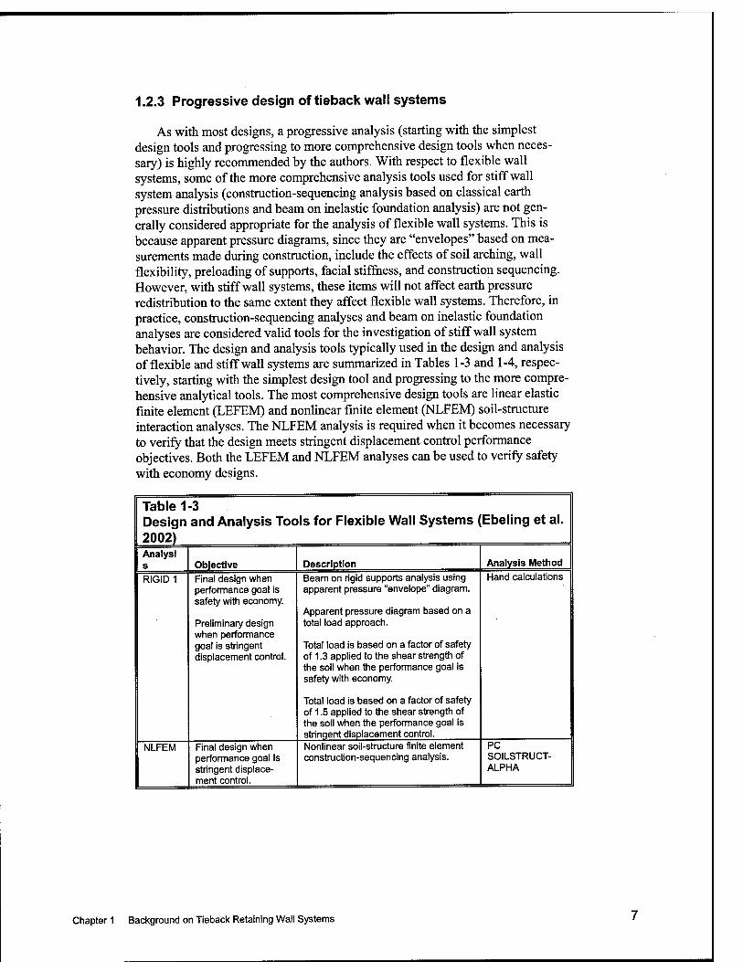
1.2.3 Progressive design of tieback wall systems
As with most designs, a progressive analysis (starting with the simplest design tools and progressing to more comprehensive design tools when neces- sary) is highly recommended by the authors. With respect to flexible wall systems, some of the more comprehensive analysis tools used for stiff wall system analysis (construction-sequencing analysis based on classical earth pressure distributions and beam on inelastic foundation analysis) are not gen- erally considered appropriate for the analysis of flexible wall systems. This is because apparent pressure diagrams, since they are "envelopes" based on mea- surements made during construction, include the effects of soil arching, wall flexibility, preloading of supports, facial stiffness, and construction sequencing. However, with stiff wall systems, these items will not affect earth pressure redistribution to the same extent they affect flexible wall systems. Therefore, in practice, construction-sequencing analyses and beam on inelastic foundation analyses are considered valid tools for the investigation of stiff wall system behavior. The design and analysis tools typically used in the design and analysis of flexible and stiff wall systems are summarized in Tables 1-3 and 1-4, respec- tively, starting with the simplest design tool and progressing to the more compre- hensive analytical tools. The most comprehensive design tools are linear elastic finite element (LEFEM) and nonlinear finite element (NLFEM) soil-structure interaction analyses. The NLFEM analysis is required when it becomes necessary to verify that the design meets stringent displacement control performance objectives. Both the LEFEM and NLFEM analyses can be used to verify safety with economy designs.
Table 1-3 Design and Analysis Tools for Flexible Wall Systems (Ebeling et al. 2002)
1 Analysi 1 s Objective Description Analysis iVIethod
RIGID 1 Final design when performance goal is safety with economy.
Preliminary design when performance goal is stringent displacement control.
Beam on rigid supports analysis using apparent pressure "envelope" diagram.
Apparent pressure diagram based on a total load approach.
Total load is based on a factor of safety of 1.3 applied to the shear strength of the soil when the performance goal is safety with economy
Total load is based on a factor of safety of 1.5 applied to the shear strength of the soil when the performance goal is stringent displacement control.
Hand calculations
NLFEM Final design when performance goal is stringent displace- ment control.
Nonlinear soli-structure finite element construction-sequencing analysis.
PC SOILSTRUCT- ALPHA
Chapter 1 Background on Tieback Retaining Wall Systems
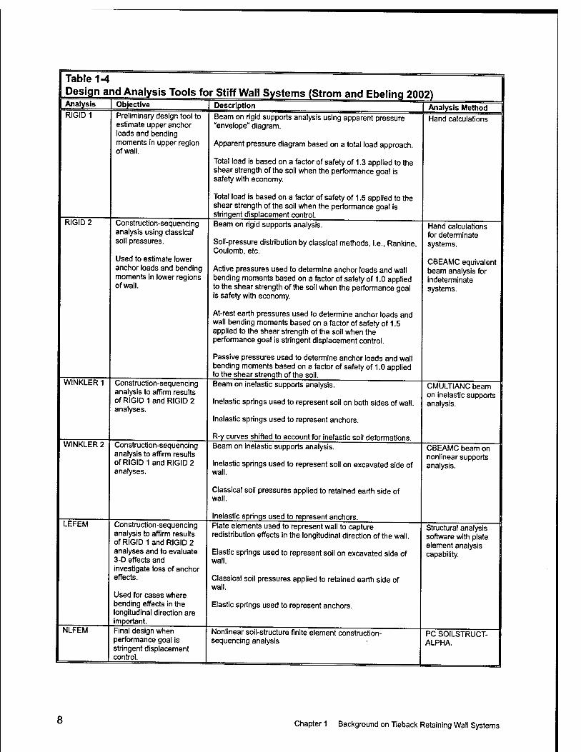
Table 1-4 Design and Analysis Tools for Stiff Wall Systems (Strom and Ebeling 2002) Analysis RIGID 1
RIGID 2
Objective
Preliminary design tool to estimate upper anchor loads and bending moments in upper region of wall.
Construction-sequencing analysis using classical soil pressures.
Used to estimate lower anchor loads and bending moments in lower regions of wall.
WINKLER 1
WINKLER 2
LEFEM
NLFEM
Description
Beam on rigid supports analysis using apparent pressure "envelope" diagram.
Apparent pressure diagram based on a total load approach.
Total load is based on a factor of safety of 1.3 applied to the shear strength of the soil when the performance goal is safety with economy
Total load is based on a factor of safety of 1.5 applied to the shear strength of the soil when the performance goal is stringent displacement control. Beam on rigid supports analysis.
Construction-sequencing analysis to affirm results of RIGID 1 and RIGID 2 analyses.
Construction-sequencing analysis to affirm results of RIGID land RIGID 2 analyses.
Construction-sequencing analysis to affirm results of RIGID land RIGID 2 analyses and to evaluate 3-D effects and investigate loss of anchor effects.
Used for cases where bending effects in the longitudinal direction are important. Final design when performance goal is stringent displacement control.
Soil-pressure distribution by classical methods, i.e., Rankine, Coulomb, etc.
Active pressures used to determine anchor loads and wall bending moments based on a factor of safety of 1.0 applied to the shear strength of the soil when the perfomiance goal is safety with economy.
At-rest earth pressures used to detennine anchor loads and wall bending moments based on a factor of safety of 1.5 applied to the shear strength of the soil when the performance goal is stringent displacement control.
Passive pressures used to determine anchor loads and wall bending moments based on a factor of safety of 1.0 applied to the shear strength of the soil. Beam on inelastic supports analysis.
inelastic springs used to represent soil on both sides of wall.
Inelastic springs used to represent anchors.
R-y curves shifted to account for inelastic soil deformations. Beam on inelastic supports analysis
inelastic springs used to represent soil on excavated side of wall.
Classical soil pressures applied to retained earth side of wall.
inelastic springs used to represent anchors. Plate elements used to represent wall to capture redistribution effects in the longitudinal direction of the wall.
Elastic springs used to represent soil on excavated side of wall.
Classical soil pressures applied to retained earth side of wall.
Elastic springs used to represent anchors.
Nonlinear soil-structure finite element construction- sequencing analysis
Analysis Method
Hand calculations
Hand calculations for determinate systems.
CBEAMC equivalent beam analysis for indeterminate systems.
CMULTIANC beam II on inelastic supports analysis.
CBEAMC beam on nonlinear supports analysis.
Structural analysis software with plate element analysis capability.
PC SOILSTRUCT- ALPHA.
Chapter 1 Background on Tieback Retaining Wall Systems
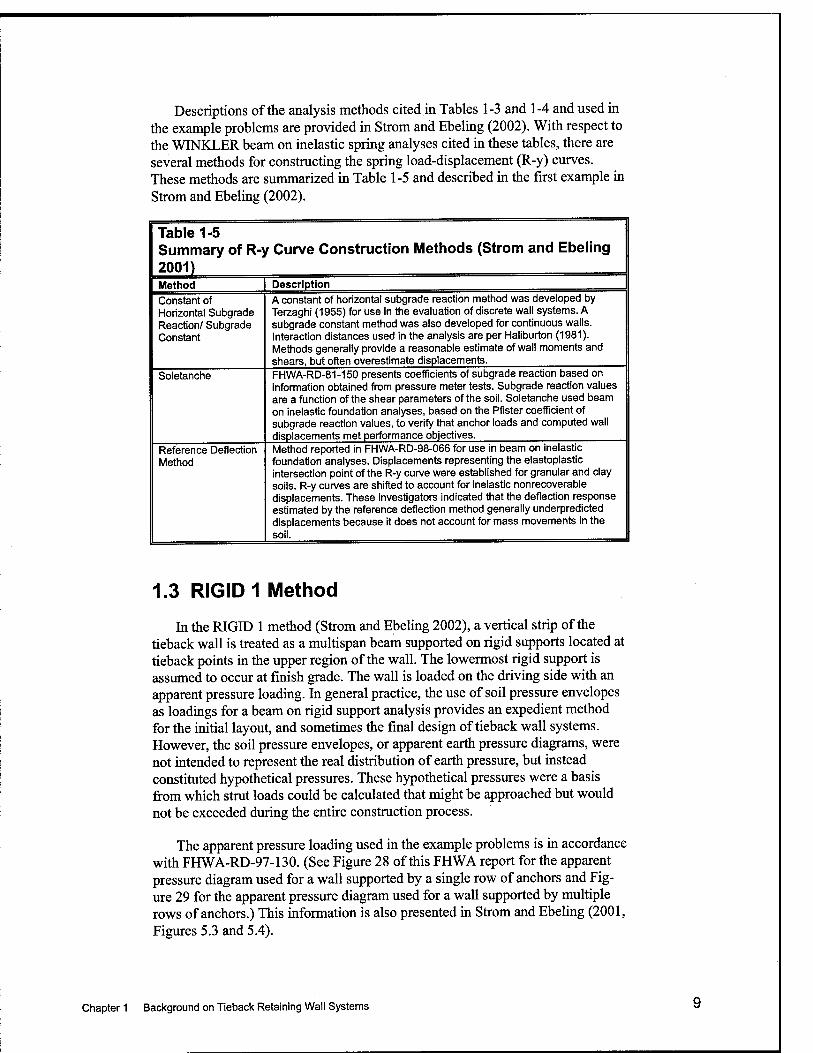
Descriptions of the analysis methods cited in Tables 1-3 and 1-4 and used in the example problems are provided in Strom and Ebeling (2002). With respect to the WINKLER beam on inelastic spring analyses cited in these tables, there are several methods for constructing the spring load-displacement (R-y) curves. These methods are summarized in Table 1-5 and described in the first example in Strom and Ebeling (2002).
Table 1-5 Summary of R-y Curve Construction Methods (Strom and Ebeling 2001) Method Constant of Horizontal Subgrade Reaction/ Subgrade Constant
Soletanche
Reference Deflection Method
Description A constant of horizontal subgrade reaction method was developed by Terzaghi (1955) for use in the evaluation of discrete wall systems. A subgrade constant method was also developed for continuous walls. Interaction distances used In the analysis are per Haliburton (1981). IVIethods generally provide a reasonable estimate of wall moments and shears, but often overestimate displacements. FHWA-RD-81-150 presents coefficients of subgrade reaction based on information obtained from pressure meter tests. Subgrade reaction values are a function of the shear parameters of the soil. Soletanche used beam on inelastic foundation analyses, based on the Pfister coefficient of subgrade reaction values, to verify that anchor loads and computed wall displacements met performance objectives. Method reported in FHWA-RD-98-066 for use in beam on inelastic foundation analyses. Displacements representing the elastoplastic intersection point of the R-y curve were established for granular and clay soils. R-y curves are shifted to account for inelastic nonrecoverable displacements. These investigators indicated that the deflection response estimated by the reference deflection method generally underpredicted displacements because it does not account for mass movements in the soil.
1.3 RIGID 1 Method
In the RIGID 1 method (Strom and Ebeling 2002), a vertical strip of the tieback wall is treated as a multispan beam supported on rigid supports located at tieback points in the upper region of the wall. The lowermost rigid support is assumed to occur at finish grade. The wall is loaded on the driving side with an apparent pressure loading. In general practice, the use of soil pressure envelopes as loadings for a beam on rigid support analysis provides an expedient method for the initial layout, and sometimes the final design of tieback wall systems. However, the soil pressure envelopes, or apparent earth pressure diagrams, were not intended to represent the real distribution of earth pressure, but instead constituted hypothetical pressures. These hypothetical pressures were a basis fi-om which strut loads could be calculated that might be approached but would not be exceeded during the entire construction process.
The apparent pressure loading used in the example problems is in accordance with FHWA-RD-97-130. (See Figure 28 of this FHWA report for the apparent pressure diagram used for a wall supported by a single row of anchors and Fig- ure 29 for the apparent pressure diagram used for a wall supported by multiple rows of anchors.) This information is also presented in Strom and Ebeling (2001, Figures 5.3 and 5.4).
Chapter 1 Background on Tieback Retaining Wall Systems
RIGID 1 design procedures are illustrated in the example problems contained in Strom and Ebeling (2002) and in the example problems in Section 10 of FHWA-RD-97-130. When tiebacks arc prestrcssed to levels consistent with active pressure conditions (i.e., Example 1 in Strom and Ebeling 2002), the total load used to determine the apparent earth pressure is based on that approximately corresponding to a factor of safety of 1.3 on the shear strength of the soil. When tiebacks are prestrcssed to minimize wall displacement (Example 2 in Strom and Ebeling 2002), the total load used to determine the apparent earth pressure is based on at-rest earth pressure coefficient conditions, or that approximately corresponding to a factor of safety of 1.5 applied to the shear strength of the soil. Empirical formulas are provided with the apparent pressure method for use in estimating anchor forces and wall bending moments.
1.4 RIGID 2 Method
As with the RIGID 1 method, a vertical strip of the tieback wall is treated as a multispan beam supported on rigid supports located at tieback points (Strom and Ebeling 2002). The lowest support location is assumed to be below the bottom of the excavation at the point of zero net pressure (Ratay 1996). Two earth pressure diagrams are used in each of the incremental excavation, anchor placement, and prestressing analyses. Active earth pressure (or at-rest earth pressure when wall displacements are critical) is applied to the driving side and extends from the top of the ground to the actual bottom of the wall. Passive earth pressure (based on a factor of safety of 1.0 applied to the shear strength of soil) is applied to the resisting side of the wall and extends from the bottom of the excavation to the actual bottom of the wall. The application of the RIGID 2 method is demonstrated in the two example problems in Strom and Ebeling (2002). The RIGID 2 method is useful for determining if the wall and anchor capacities determined by the RIGID 1 analysis are adequate for stiff tieback wall systems, and permits redesign of both flexible and stiff tieback wall systems to ensure that strength is adequate for all stages of construction. No useful informa- tion can be obtained from the RIGID 2 analysis regarding displacement demands, however.
1.5 WINKLER1 Method
The WINKLER 1 method (described in Strom and Ebeling 2002) uses idealized elastoplastic springs to represent soil load-deformation response and anchor springs to represent ground anchor load-deformation response. The elastoplastic curves (R-y curves) representing the soil springs for the example problems are based on the reference deflection method (FHWA-RD-98-066). Other methods are available for developing elastoplastic R-y curves for beam on inelastic foundation analyses. The reference deflection method (FHWA-RD-98- 066), the Haliburton (1981) method, and the Pfister method (FHWA-RD-81-150) are described in the first example problem. Elastoplastic curves can be shifted with respect to the undeflected position of the tieback wall to capture non- recoverable plastic movements that may occur in the soil during various con- struction stages (e.g., excavating, anchor placement, and prestressing of anchors).
' ^ Chapter 1 Background on Tieback Retaining Wall Systems
This R-y curve shifting was used in both example problems to consider the non- recoverable active state yielding that occurs in the retained soil during the first- stage excavation (cantilever-stage excavation). The R-y curve shift following the first-stage excavation will help to capture the increase in earth pressure that occurs behind the wall as anchor prestress is applied, and as second-stage excava- tion takes place. In the two example problems in Strom and Ebeling (2002), once the upper anchor is installed, the second-stage excavation causes the upper section of the tieback wall to deflect into the retained soil—soil that has previ- ously experienced active state yielding during first-stage excavation. The WINKLER 1 method is useful for determining if the wall and anchor capacities determined by a RIGID 1 or RIGID 2 analysis are adequate, and permits redesign of stiff tieback wall systems to ensure that strength is adequate for all stages of construction. It also provides usefiil information on "relative" displacement demands and facihtates redesign of the wall system when it becomes necessary to meet displacement-based performance objectives.
The PC-based computer program CMULTIANC used to simulate the simplified construction sequence in the analysis of a stiff tieback wall is classified as a WINKLER 1 type analysis by Strom and Ebeling (2002). Top- down construction is assumed in this analysis procedure. This report presents three abbreviated example analyses. Strom and Ebeling (2002) compare the resuhs from CMULTIANC and other methods of analysis for two of the example tieback walls (the Soletanche wall and Bonneville wall analyses) contained within this report.
1.6 WINKLER 2 Method
The WINKLER 2 method (Strom and Ebeling 2002) is a simple beam on inelastic foundation method that uses soil loadings on the driving side of the wall and elastoplastic soil springs on the resisting side of the wall in an incremental excavation, anchor placement, and anchor prestressing analysis. As with the WINKLER 1 method, the elastoplastic curves representing the soil springs are based on the reference deflection method, and anchor springs are used to represent the ground anchor load-deformation response. However, the WINKLER 2 method is unable to capture the effects of nonrecoverable plastic movements that may occur in the soil during various construction stages. Although not considered to be as reUable as the WINKLER 1 method, the WINKLER 2 method is usefiil for determining if the wall and anchor capacities determined by a RIGID 1 or RIGID 2 analysis are adequate, and the method permits redesign of stiff tieback wall systems to ensure that strength is adequate for all stages of construction. It also provides information on relative displace- ment demands (i.e., the effects of system alterations described in terms of changes in computed displacements) and permits redesign of the wall system to meet stringent displacement control performance objectives.
^ At this time, the authors of this report do not propose to use WINKLER inelastic spring-based methods of analyses to predict wall displacements. However, the differences in the computed deformations of an altered wall system based on WINKLER analyses may be useful as a qualitative assessment of change in stiffness effects.
Chapter 1 Background on Tieback Retaining Wall Systems 11
1.7 NLFEM Method
When displacements are important with respect to project performance objectives, a nonlinear finite element soil-structure interaction (SSI) analysis should be performed. In an NLFEM analysis, soil material nonlinearities are considered. Displacements are often of interest when displacement control is required to prevent damage to structures and utilities adjacent to the excavation. To keep displacements within acceptable limits, it may be necessary to increase the level of prestressing beyond that required for basic strength performance. An increase in tieback prestressing is often accompanied by a reduction in tieback spacing. As tieback prestressing is increased, wall lateral movements and ground surface settlements decrease. Associated with an increased level of prestress is an increase in soil pressures. The higher soil pressures increase demands on the structural components of the tieback wall system. General-purpose NLFEM programs for two-dimensional plane strain analyses of SSI problems are available (e.g., PC-SOILSTRUCT-ALPHA) to assess displacement demands on tieback wall systems. These programs can calculate displacements and stresses due to incremental construction and/or load application and are capable of modeling nonlinear stress-strain material behavior. An accurate representation of the nonlinear stress/strain behavior of the soil, as well as proper simulation of the actual (incremental) construction process (excavation, anchor installation, anchor prestress, etc.), in the finite element model is essential if this type of analysis is to provide meaningful results. This type of analysis is referred to as a complete construction sequence analysis (versus the simplified construction sequence analysis of CMULTIANC). See Strom and Ebeling (2001) for additional details regarding nonlinear SSI computer programs for displacement prediction.
1.8 Factors Affecting Analysis Methods and Results
1.8.1 Overexcavation
Overexcavation below ground anchor support locations is required to provide space for equipment used to install the ground anchors. It is imperative that the specified construction sequence and excavation methods are adhered to and that overexcavation below the elevation of each anchor is limited to a maximum of 2 ft. Construction inspection requirements in FHWA-SA-99-015 require inspec- tors to ensure that overexcavation below the elevation of each anchor is limited to 2 ft, or as defined in the specifications. In the Bonneville temporary tieback wall example, an overexcavation of 5.5 ft was considered for the initial design. This should be a "red flag" to the designer that a construction-sequencing evaluation is needed, and that such an evaluation will likely demonstrate that the maximum force demands on the wall and tiebacks will occur during intermediate stages of construction rather than for the final permanent loading condition. For additional information on the effect of overexcavation on tieback wall performance, see Yoo (2001).
12 Chapter 1 Background on Tieback Retaining Wall Systems
1.8.2 Ground anchor preloading
Unless anchored walls are prestressed to specific active stress levels and their movement is consistent with the requirements of the active condition at each construction stage, the lateral earth pressure distribution will be essentially non- linear with depth, and largely determined by the interaction of local factors. These may include soil type, degree of fixity or restraint at the top and bottom, wall stiffness, special loads, and construction procedures (Xanthakos 1991). To ensure that ground anchor prestressing is consistent with active state conditions, the designer will generally limit anchor prestress to values that are between 70 and 80 percent of those determined using an equivalent beam on rigid supports analysis based on apparent pressure loadings (FHWA-RD-81-150). However, this may produce wall movements toward the excavation that are larger than tolerable, especially in cases where structures critical to settlement are founded adjacent to the excavation. Larger anchor prestressed loads are generally used when structures critical to settlement are founded adjacent to the excavation. Selection of an arbitrary prestress load can be avoided by using the WINKLER 1 method beam on inelastic foundation analysis described previously. This type of analysis permits the designer to relate wall movement to anchor prestress and/or anchor spacing in order to produce tieback wall performance that is consistent with displacement performance objectives.
1.9 Construction Long-Term, Construction Short-Term, and Postconstruction Conditions
For a free-draining granular backfill, the pore-water pressure does not usually include excess pore-water pressures generated in the soil by changes in the total stress regime due to construction activities (excavation, etc.). This is because the rate of construction is much slower than the ability of a pervious and firee- draining granular soil to rapidly dissipate construction-induced excess pore-water pressures.
However, for sites containing soils of low permeabiUty (soils that drain slower than the rate of excavation/construction), the total pore-water pressures will not have the time to reach a steady-state condition during the construction period. In these types of slow-draining, less permeable soils (often referred to as cohesive soils), the shear strength of the soil during wall construction is often characterized in terms of its undrained shear strength. The horizontal earth pressures are often computed using values of the undrained shear strength for these types of soils, especially during the short-term, construction loading condi- tion (sometimes designated as the undrained loading condition—^where the term xmdrained pertains to the state within the soil during this stage of loading).
As time progresses, however, walls retained in these types of soils can vmdergo two other stages of construction loading: the construction long-term (drained or partially drained) condition and the postconstruction/permanent (drained) condition. Under certain circumstances, earth pressures may be com- puted in poorly drained soils using the Mohr-Coulomb (effective stress-based) shear strength parameter values for the latter load case(s).
Chapter 1 Background on Tieback Retaining Wall Systems ' 3
Liao and Neff (1990), along with others, point out that all three stages of loading must be considered when designing tieback wall systems, regardless of soil type. As stated previously, for granular soils, the construction short- and long-term conditions are usually synonymous since drainage in these soils occurs rapidly. Differences in the construction short- and long-term conditions are gen- erally significant only for cohesive soils. Changes in the groundwater level (if present) before and after anchor wall construction, as well as postconstruction/ permanent, must be considered in these evaluations. Designers must work closely with geotechnical engineers to develop a soils testing program that will produce soil strength parameters representative of each condition—construction short term, construction long term, and postconstruction. The program should address both laboratory and field testing requirements. Additional information on con- struction short-term, construction long-term, and postconstruction condition earth-pressure loadings can be found in Strom and Ebeling (2001). Methods used to estimate long-term (drained) shear strength parameters for stiff clay sites are presented in Appendix A of Strom and Ebeling (2002).
1.10 Construction-Sequencing Analyses
Tieback wall design procedures vary in practice, depending on whether the tieback wall is considered to be flexible or stiff Flexible wall systems include the following:
• Vertical sheet-pile systems.
• Soldier beam and lagging systems.
As stated previously, flexible wall systems are often designed using an equivalent beam on rigid support method of analysis with an apparent earth pressure envelope loading. The flexible wall system design approach is illustrated herein with respect to the two stiff tieback wall examples in Strom and Ebeling (2002) in order to be able to compare the results with those obtained using the simplified construction-sequencing type analyses (of CMULTIANC). The flexible wall design process is also illustrated in Ebeling et al. (2002).
Stiff tieback wall systems include the following:
• Secant cylinder pile systems.
• Continuous reinforced concrete (tremie wall) systems.
• Soldier beam-tremie wall systems.
In practice, the stiff tieback wall systems employ some type of construction- sequencing analysis, i.e., staging analysis, in which the anchor loads, wall bending moments, and possibly wall deflections are determined for each con- struction stage. In general, designers recommend against application of the apparent pressure diagram approach, used for flexible tieback wall systems, for the design of stiff tieback wall systems (Kerr and Tamaro 1990). Equivalent beam on rigid support methods and beam on inelastic foundation methods are
14 Chapter 1 Background on Tieback Retaining Wall Systems
those methods most commonly used in the construction-sequencing analysis. Classical earth pressure theories (Rankine, Coulomb, etc.) are generally used in the equivalent beam on rigid support method. Profiles of lateral earth pressures on both sides of the wall are developed by classical theory with active pressures acting on the driving side and passive pressures acting on the resisting side. An at-rest pressure profile may be used to represent driving side earth pressures for stiff wall systems that are required to meet stringent displacement performance objectives. The beam on inelastic foundation method allows displacement performance to be assessed directly (in a relative but not an absolute sense). It is therefore preferred over the equivalent beam on rigid support method for tieback wall systems where displacement performance is critical. Both the equivalent beam on rigid support method and the beam on inelastic foundation method are demonstrated in a simplified construction-sequencing analysis with respect to the design and evaluation of two stiff tieback wall systems in Strom and Ebeling (2002). Two of these example CMULTIANC analyses are presented in this report.
Chapter 1 Background on Tieback Retaining Wall Systems 15
2 Computer Program CMULTIANC
2.1 Introduction
This report describes the computer program CMULTIANC, which performs analyses simulating the construction sequence of a stiff, multiply anchored tie- back wall. "Stiff walls are described by Strom and Ebeling (2001, 2002). The analyses are performed using a one-dimensional finite element method described by Dawkins (1994a, 1994b).
2.2 Disclaimer
The program is based on criteria provided by the Information Technology Laboratory, Vicksburg, MS, U.S. Army Engineer Research and Development Center. The program has been checked within reasonable limits to assure that the results are accurate within the limitations of the procedures employed. However, there may exist combinations of parameters which may cause the program to produce questionable results. It is the responsibility of the user to judge the validity of the results reported by the program. The author assumes no responsi- bility for the design or performance of any system based on the results of this program.
2.3 System Overview
The procedures employed in this program are applicable to stiff anchored tieback walls as described in Strom and Ebeling (2001, 2002).
The general wall/soil system shown in Figure 2-1 may be used for either cantilever or anchored walls. The system is assumed to be uniform perpendicular to the plane of the figure. A typical 1-ft slice of the uniform system is used for analysis.
16 Chapter 2 Computer Program CMULTIANC
Line Load-\ Surcharge Load
\
1 ^^
,^ Soil Layer-^
^Lauier Boundarv
^^.
1^ '
/-Soil Layer-^
WaterSurface-^
- ^WaterSurface ^SoilLayer-^
Layer Boundary ^ ^ Layer Boundary
7" /-Soil Layer ^
^ Soil Layer ^
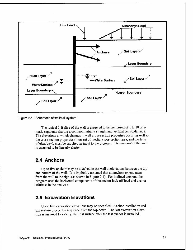
Figure 2-1. Schematic of wall/soil system
The typical 1-ft slice of the wall is assumed to be composed of 1 to 10 pris- matic segments sharing a common initially straight and vertical centroidal axis. The elevations at which changes in wall cross-section properties occur, as well as the cross-section properties (moment of inertia, cross-section area, and modulus of elasticity), must be supplied as input to the program. The material of the wall is assumed to be linearly elastic.
2.4 Anchors
Up to five anchors may be attached to the wall at elevations between the top and bottom of the wall. It is implicitly assumed that all anchors extend away from the wall to the right (as shown in Figure 2-1). For inclined anchors, the program uses the horizontal components of the anchor lock-offload and anchor stiffness in the analysis.
2.5 Excavation Elevations
Up to five excavation elevations may be specified. Anchor installation and excavation proceed in sequence from the top down. The last excavation eleva- tion is assumed to specify the final surface after the last anchor is installed.
Chapter 2 Computer Program CMULTIANC 17
2.6 Soil Profile
A different soil profile, composed of 1 to 11 distinct layers, is assumed to exist on either side of the wall. Boundaries between subsurface layers are assumed to be straight horizontal lines. Soil layers are assumed to extend ad infinitum away from the wall. The lowest layer described on either side of the wall is assumed to extend ad infinitum downward.
2.6.1 Unit weights
Each layer is characterized by two unit weights: moist and saturated.
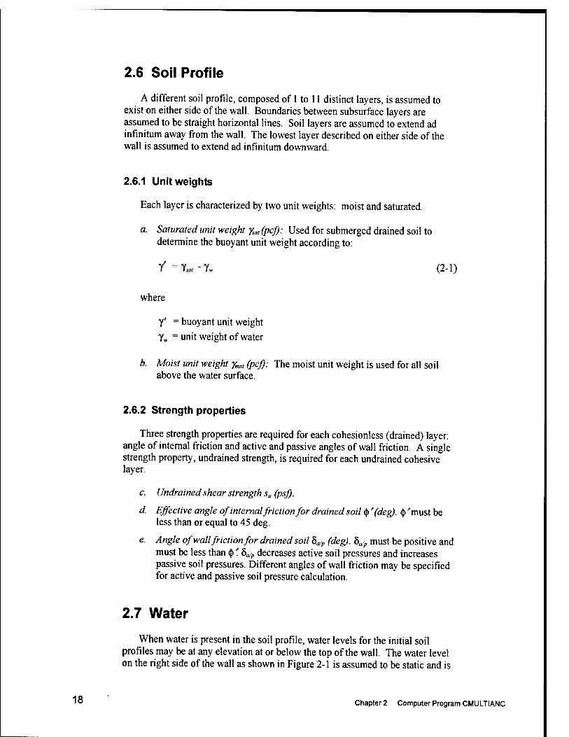
a. Saturated unit weight %at (pcj): Used for submerged drained soil to determine the buoyant unit weight according to:
i = Isa, - YH. (2-1)
where
Y' = buoyant unit weight
Y^ = unit weight of water
b. Moist unit weight y„^„ (pcJ): The moist unit weight is used for all soil above the water surface.
2.6.2 Strength properties
Three strength properties are required for each cohesionless (drained) layer: angle of internal friction and active and passive angles of wall friction. A single strength property, undrained strength, is required for each undrained cohesive layer.
c. Undrained shear strength 5„ (psj).
d. Effective angle of internal friction for drained soil fy '(deg). ^ 'must be less than or equal to 45 deg.
e. Angle of wall friction for drained soil ha'p (deg). 5^p must be positive and must be less than ^'. hajp decreases active soil pressures and increases passive soil pressures. Different angles of wall friction may be specified for active and passive soil pressure calculation.
2.7 Water
When water is present in the soil profile, water levels for the initial soil profiles may be at any elevation at or below the top of the wall. The water level on the right side of the wall as shown in Figure 2-1 is assumed to be static and is
' ° Chapter 2 Computer Program CMULTIANC
unchanged during the construction sequence. Water elevations on the left side must also be specified for each excavation described for the construction sequence. The water elevation for an excavation must be at or below the initial water elevation on the left side and at or below the elevation specified for the previous excavation.
2.8 Vertical Surcharge Loads
Vertical surcharge loads may be applied as line loads or distributed loads to the right-side surface:
a. Line loads. Vertical line loads may be applied to the right-side surface.
b. Distributed loads. Five distributed load variations are available:
(1) Uniform load. A uniform surcharge is constant and extends ad infinitum over the entire soil surface. Only one uniform load may be prescribed on the right-side surface.
(2) Strip loads. Strip loads are uniformly distributed over a finite segment of the soil surface. Several strip loads may be applied to the right-side surface.
(3) Ramp load. A ramp load begins at zero at some distance fi-om the wall, increases linearly to a maximum value, and continues ad infinitum as a uniform load. Only one ramp load may be applied to the right-side surface.
(4) Triangular loads. A triangular load begins at zero at some distance from the wall, increases linearly to a maximum, then decreases to linearly to zero. Several triangular loads may be applied to the right- side surface.
(5) Variable distributed load. A variable distributed loading is described by a sequence of distance/load points. The load is assumed to vary linearly between adjacent points.
2.9 Limiting Soil and Water Pressures
Horizontal loads are imposed on the structure by the surrounding soil (including the effects of surface surcharges), the effects of anchors, and water. Water pressures are unaffected by displacements. Soil pressures depend on both the magnitude and direction of wall displacements and vary between limiting active and passive pressures.
2.10 Calculation Points
Force magnitudes and wall response are calculated at the following points:
Chapter 2 Computer Program CMULTIANC '"
a. At 1-ft intervals beginning at the top of the wall.
b. At the top and bottom of the wall and at the locations of changes in cross section.
c. At the intersection of the soil surface and soil layer boundaries on each side of the wall.
d At the intersection of the water surface on each side of the wall.
e. At the location of the anchors.
/ At other locations to establish the resultant force or pressure distribution as necessary for the analysis.
2.11 Active and Passive Pressures
2.11.1 Undrained (cohesive) soils
Active and passive soil pressures,/?^A and/?/./,, respectively, in a homogeneous undrained (cohesive) soil profile are calculated from:
PAH = P.-2s„ (2-2)
Pph =Pv + 2s ^ (2-3)
where pv, is the cumulative vertical pressure using y^^ for soil above water
a"<iy.«ft>r submerged soil plus any uniform surcharge.
2.11.2 Drained (cohesioniess) soils
Active and passive soil pressures for a homogeneous drained (cohesioniess) soil profile are calculated using earth pressure coefficients as described in the next section.
2.11.3 Pressure coefficients
The earth pressure coefficients are given by:
a. Active coefficient:
K,= COS(j)
j^ |sin(<t) + 5Jsin(t)
cos5„
cos 5„ (2-4)
20 Chapter 2 Computer Program CMULTIANC
b. Passive coefficient for bp <^I2:
Kp = coscj)
|sin((|) + 5^)sin(j) 1-.
cos 8„
cos5„ (2-5)
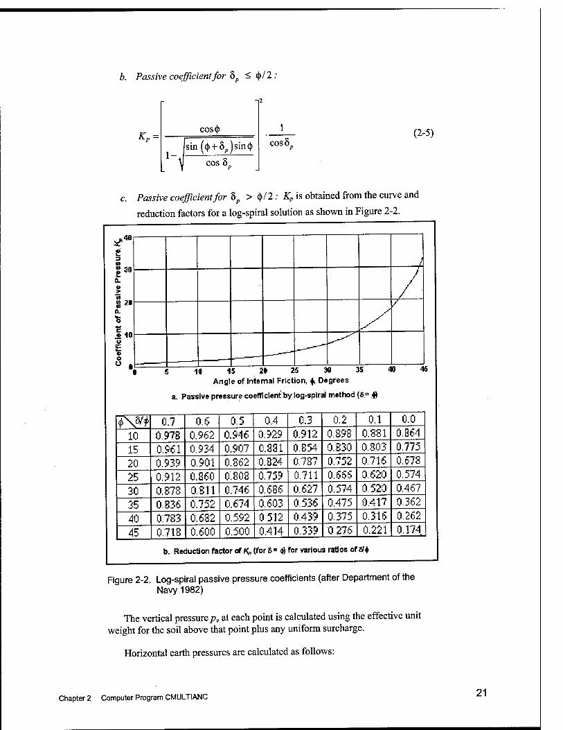
c. Passive coefficient for 5^ > ^/2: Kp is obtained from the curve and
reduction factors for a log-spiral solution as shown in Figure 2-2.
3 n
Q.
S2" <L <■- O
■ **
« 10 u E » o O
10 Angle of Internal Friction, ^ Degrees
a. Passive pressure coefficient by log-spiral method (5= ♦)
<f^\^^ 0.7 0.6 0,5 0.4 0.3 0.2 0,1 0,0
10 0.97S 0.962 0.946 0.929 0.912 0.898 0.881 0,864
15 0.961 0.934 0.907 0.881 0.854 0.830 0,803 0,775
20 0.939 0.901 0.862 0.824 0.787 0.752 0,715 0,678
25 0.912 0.860 0.808 0.759 0.711 0.556 0,520 0,574
30 0.878 0.811 0.746 0,686 0.527 0.574 0,520 0,467
35 0.836 0.752 0.674 0.603 0.535 0.475 0,417 0,362
40 0.783 0.682 0.592 0,512 0.439 0.375 0,315 0,262
45 0.718 0.600 0.500 0.414 0.339 0,275 0.221 0,174
b. Reduction factor of K^ (for S= (t>) for various ratios of 6f*
Figure 2-2. Log-spiral passive pressure coefficients (after Department of the Navy 1982)
The vertical pressure/^v at each point is calculated using the effective unit weight for the soil above that point plus any uniform surcharge.
Horizontal earth pressures are calculated as follows:
Chapter 2 Computer Program CMULTIANC 21
22
a. A ctive pressures.
PAh = K^-p^-cosbp (2-6)
b. Passive pressures.
Pph= ^p-Py-cosd^ (2-7)
2.11.4 Profiles with interspersed undrained and drained layers
When a change in either (|), s„, or unit weight occurs at a boundary between layers, dual pressure values are calculated using the soil properties above and below the boundary. The vertical pressure increases with total unit soil weight in undrained (cohesive) layers and with effective unit weight in drained (cohesion- less) layers.
2.11.5 Pressures due to surcharge loads
The contribution of surcharges (other than a uniform surcharge) to horizontal pressures is calculated from the theory of elasticity according to Figure 2-3.
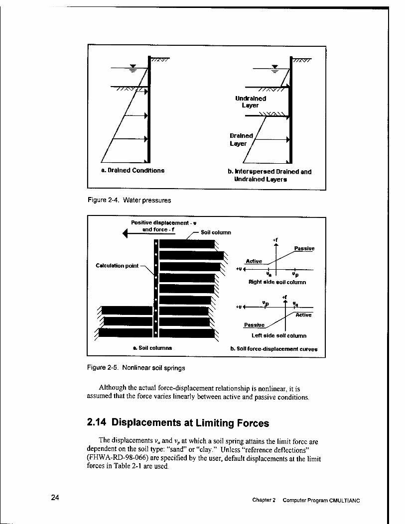
2.12 Water Pressures
Hydrostatic pressures arc applied to the wall when the water level on either side is above the bottom of the wall and the soil is drained. Water pressures in undrained soils are incorporated in the soil pressures, and additional water pressures in undrained layers are set to zero. Potential water pressure distri- butions are illustrated in Figure 2-4.
2.13 Nonlinear Soil and Anchor Springs
The soil pressure or anchor force exerted on the wall at any point is assumed to depend only on the displacement at that point (i.e., the Winkler assumption). In effect, the Winkler assumption results in treating the soil and anchors as isolated translation resisting elements.
Under the Winkler assumption, the soil system may be visualized as a system of independent columns with curves representing the soil pressure-displacement relationship for the soil columns as shown in Figure 2-5.
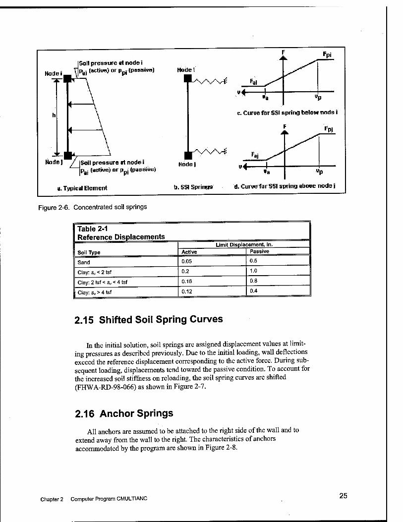
Soil-structure interaction at each node is represented by two concentrated springs with characteristics obtained from soil pressures immediately above and below the node as illustrated in Figure 2-6 for the soil on the right side.
Limiting forces are calculated as follows:
Chapter 2 Computer Program CMULTIANC
mH
nH
I. Line Loads
MfiW m > 0.4
^ ♦P
ml 1.4 P /" 1.203 n ^
•* H\.(0.1B*n2>2j
•l •2 * »in*ico»*i- slnSjeosej } ^(Q; Ql) r co^ .sin3»i.«ln2*2l
b. KstrlHited Loads
Figure 2-3. Pressure calculations for surcharge loads
a. For the curve below node i:
h Fa> = -^{^'Pa^ ^P<^) (2-8)
Pp> = T{^'Ppi + P.j) (2-9)
b. For the curve above nodej:
F, = -(p, + 2.pJ (2-10)
Ppj = l(Ppi^^'P^) (2-11)
Chapter 2 Computer Program CMULTIANC 23
TTT^^yrr^ 777^^77 Undrained
Layer
Drained. Layer
■777^77
a. Drained Conditions b. Interspersed Drained and Undrained Layers
Figure 2-4. Water pressures
Positive displacement - g and force - f Soil column
Active +V4-
Passive
Rigtit side soil column
+f
+v^ Active
a. Soil columns
Passive
Left side soil column
b. Soil force-displacement curves
Figure 2-5. Nonlinear soil springs
Although the actual force-displacement relationship is nonlinear, it is assumed that the force varies linearly between active and passive conditions.
2.14 Displacements at Limiting Forces
The displacements v^ and Vp at which a soil spring attains the limit force are dependent on the soil type: "sand" or "clay." Unless "reference deflections" (FHWA-RD-98-066) are specified by the user, default displacements at the limit forces in Table 2-1 are used.
24 Chapter 2 Computer Program CMULTIANC
tkidei,
Soil pressure at nodei Pgj (active) or Ppj (passiiie)
Hadej /jSoil pressurett nodei Pgj (active) or Ppj (passive)
a. Typical Element
Figure 2-6. Concentrated soil springs
Hade J
hi vi—^■
c. Curve far SSI spring below node i
b. SSI Springs d. Curve far SSI spring abose node j
Table 2-1 Reference Displacements
Soil Type
Limit Displacement, in. || Active Passive
Sand 0.05 0.5
Clay: s„ < 2 tsf 0.2 1.0
Clay: 2 tsf < s„ < 4 tsf 0.16 0.8
1 Clay: s„ > 4 tsf 0.12 0.4 ■ ■■,„„ , ■;;;i^;j.
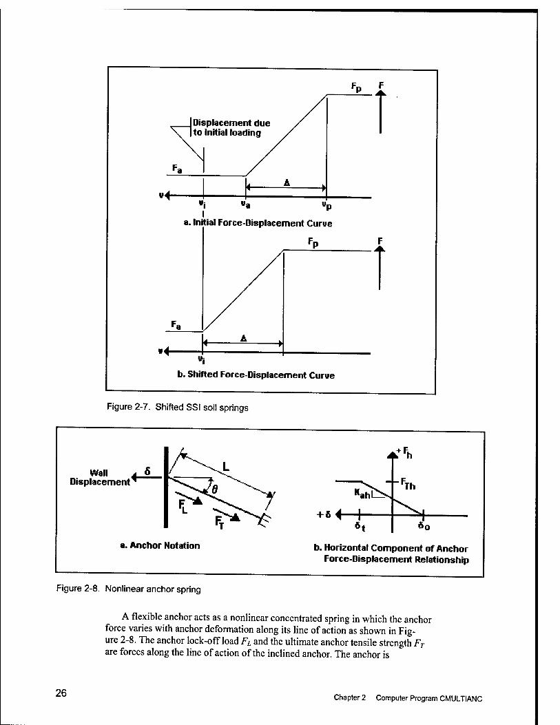
2.15 Shifted Soil Spring Curves
In the initial solution, soil springs are assigned displacement values at limit- ing pressures as described previously. Due to the initial loading, wall deflections exceed the reference displacement corresponding to the active force. During sub- sequent loading, displacements tend toward the passive condition. To account for the increased soil stiffness on reloading, the soil spring curves are shifted (FHWA-RD-98-066) as shown in Figure 2-7.
2.16 Anciior Springs
All anchors are assumed to be attached to the right side of the wall and to extend away from the wall to the right. The characteristics of anchors accommodated by the program are shown in Figure 2-8.
Chapter 2 Computer Program CMULTIANC 25
Displacement due initial loading
«4- I
a. Initial Force-Displacement Curve
"4-
b. Shifted Force-Displacement Curve
Figure 2-7. Shifted SSI soil springs
Wall Displacement 4-
F
I
-^^•^h
--F,
■^aiiL^
+ 5^-4-
Th
a. Anchor Notation b. Horizontal Component of Anchor Force-Displacement Relationship
Figure 2-8. Nonlinear anchor spring
A flexible anchor acts as a nonlinear concentrated spring in which the anchor force varies with anchor deformation along its line of action as shown in Fig- ure 2-8. The anchor lock-offload FL and the ultimate anchor tensile strength FT are forces along the line of action of the inclined anchor. The anchor is
26 Chapter 2 Computer Program CMULTIANC
characterized by the properties modulus of elasticity E, cross-section area A, effective length L, slope 6, and plan spacing between adjacent anchors s.
CMULTIANC deals only with horizontal displacement of the wall. Conse- quently, the force-displacement relationship for the anchor spring must be expressed by the horizontal components of anchor force and spring stiffness. During the construction sequence simulation, a force equal to the horizontal component of the anchor lock-offload (Fi cos 0) is applied at the point of anchor attachment. After the displacements due to the lock-offload are determined, the lock-offload is replaced by a nonlinear concentrated anchor spring. The force- deformation relationships for the anchor spring are obtained from the following expressions.
The horizontal component of the anchor spring stiffness per foot of wall is given by
Ls "-ah cos'e (2-12)
Defining displacements for the anchor spring force-displacement relationship
are given by
6„ = 5, - F,, I K^ (2-13)
6, = 8„ + F^ / K^, (2-14)
where
s
is the horizontal component of the anchor lock-offload per foot of wall,
Fj^=^cose s
is the horizontal component of the anchor ultimate strength
5i = lateral displacement of the point of attachment from the solution with the anchor lock-offload Fa applied.
For deformation beyond 8,, the anchor force is constant at Fn- For deforma- tions intermediate to 5, and 5<„ the anchor force-deformation relationship may be represented as a combination of a concentrated force and a linear concentrated spring. The anchor force and displacement reported by the program are com- ponents along the line of action of the anchor. The reported anchor force is the TOTAL (NOT per foot of wall) force in the anchor.
Chapter 2 Computer Program CMULTIANC 27
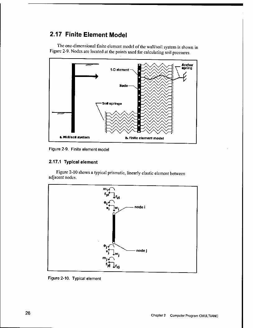
2.17 Finite Element IVIodel
The one-dimensional finite element model of the wall/soil system is shown in Figure 2-9. Nodes are located at the points used for calculating soil pressures.
Figure 2-9. Finite element model
2.17.1 Typical element
Figure 2-10 shows a typical prismatic, linearly elastic element between adjacent nodes.
Figure 2-10. Typical element
28 Chapter 2 Computer Program CMULTIANC
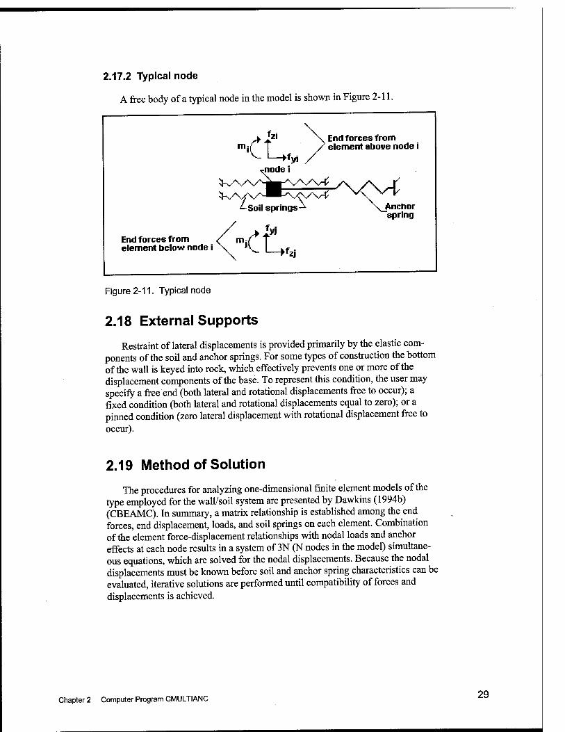
2.17.2 Typical node
A free body of a typical node in the model is shown in Figure 2-11.
End forces from element below node I
End forces from element aboue node i
■^XC^ Anchor 'spring
Figure 2-11. Typical node
2.18 External Supports
Restraint of lateral displacements is provided primarily by the elastic com- ponents of the soil and anchor springs. For some types of construction the bottom of the wall is keyed into rock, which effectively prevents one or more of the displacement components of the base. To represent this condition, the user may specify a free end (both lateral and rotational displacements free to occur); a fixed condition (both lateral and rotational displacements equal to zero); or a pinned condition (zero lateral displacement with rotational displacement free to occur).
2.19 Method of Solution
The procedures for analyzing one-dimensional finite element models of the type employed for the wall/soil system are presented by Dawkins (1994b) (CBEAMC). In summary, a matrix relationship is established among the end forces, end displacement, loads, and soil springs on each element. Combination of the element force-displacement relationships with nodal loads and anchor effects at each node results in a system of 3N (N nodes in the model) simultane- ous equations, which are solved for the nodal displacements. Because the nodal displacements must be known before soil and anchor spring characteristics can be evaluated, iterative solutions are performed until compatibility offerees and displacements is achieved.
Chapter 2 Computer Program CMULTIANC 29
30
2.20 Stability of Solution
If the nodal displacements arc excessive, the elastic component of the soil and/or anchor springs may not be present. If all elastic restraint against lateral displacement is lost, the wall/soil system is unstable. The program checks for "reasonable" displacements during each iteration and terminates execution if instability is indicated.
2.21 Computer Program
The computer program CMULTIANC is menu driven to provide flexibility of control. Input data may be provided from a predefined data file or from the user's keyboard during execution. Input data may be edited from the keyboard at any time. The program generates input and output files as well as providing for graphical display of input data and results of the solution.
The menu on the main screen consists of the follov^'ing main and submenu items:
a. File Menu: The File Menu comprises the following submenu items:
(1) New: Allows saving any unsaved input or output data; initializes and/or erases all data variables.
(2) Open: Allows saving any unsaved input or output data; initializes and/or erases all data variables; displays the Open File dialog box to permit a predefined input data file to be read.
(3) Save: Allows saving any input and/or output data files at any time.
(4) Print: Allows the input and/or output files to be printed at any time.
(5) Exit: Allows saving any unsaved input or output data; terminates execution and unloads CMULTIANC.
b. Edit Menu: Allows saving any unsaved input or output data; permits editing and/or entering input data from the user's keyboard.
c. View Menu: The View Menu comprises the following submenu items:
(1) Current Input File: Displays the current input data in Input Data File format.
(2) Output File: Displays the current output file.
(3) Input Plots: Displays schematics of system geometry, surface surcharges, and horizontal loads.
(4) Limiting Soil and Water Pressures: Displays graphs of active and passive soil pressures and net water pressure.
Chapter 2 Computer Program CMULTIANC
(5) Results Plots: Displays graphs of deflections, moment diagram, shear diagram, and final soil pressures.
d. Solve Menu: Initiates solution of the problem and allows stepping through the construction sequence with the following submenu items:
(1) Generate Limiting Soil Pressures and SSI curves.
(2) Solve for Initial Displacements.
(3) Shift SSI Curves.
(4) Solve with Shifted SSI Curves.
(5) Install Anchors in Sequence.
(6) Evaluate Effects of Excavation in Sequence.
e. Help Menu: Invokes the CMULTIANC Help File.
2.22 Input Data Files
Input data may be supplied from a predefined permanent file or fi-om the user's keyboard during execution. Input data are described in Appendix A, and an abbreviated input guide is given in Appendix B. Whenever data are entered from the keyboard, either initially or by editing existing data, the program generates a temporary file in input file format for storing the data. The temporary file may be saved as a permanent file at any time. Unless the temporary file is saved, existing input is lost when the program is exited or when existing data are edited during execution.
2.23 Output Data File
As soon as input data are read from a permanent file or entered firom the keyboard, a temporary output file is generated. The temporary output file may be saved as a permanent file at any time during execution. Unless the temporary output file is saved as a permanent file, output data will be lost when the program is exited or when new input data are provided. The temporary (permanent) output file contains the following information:
a. Echoprint of input data: Presents a listing of input data with headings and appropriate units. The echoprint is automatically generated on completion of input.
b. Limiting soil and water pressures: As soon as active and passive soil pressures on each side of the wall and water pressures have been calcu- lated, a tabular listing of these data is added to the temporary output file.
c. SSI curve data: At each stage of the construction sequence, current SSI curve data are added to the output file.
Chapter 2 Computer Program CMULTIANC 31
32
d. Results of solution: As soon as the solution for each stage of the con- struction sequence has been successfully completed, a complete tabula- tion of results is appended to the output file. This tabulation contains a summary of maximum axial and lateral displacements, bending moment, shear, and soil pressures and a listing of lateral and axial displacements, axial force, shear force, bending moment, and left-side and right-side soil pressure at each calculation point.
2.24 Graphics
The following graphic displays of input data are provided by the program:
a. System: A schematic showing the wall, any anchors, the soil surface, soil layer boundaries, and water levels on each side of the wall.
b. Surcharge Loads: Schematics of vertical line, uniform, strip, ramp, triangular, and/or variable loads applied to the soil surface.
c. Limiting Soil and Water Pressures: Plots of active, at-rest, and passive soil pressures for each side of the wall and net water pressures when water elevation data are provided.
d. Results: Following a successful solution, plots are available for lateral displacements, shear forces, bending moments, and final soil pressures throughout the length of the wall.
2.25 Construction Sequence Simulation
2.25.1 Input data
It is assumed that the input data, whether entered from the keyboard or from a data file, contain data for all system components including anchors to be installed and excavation elevations to be encountered during the construction sequence.
The soil profile for the right side is unchanged during the construction sequence. The initial soil surface for the left side is assumed to be below the elevation of the topmost anchor. The left-side profile will be revised as the construction sequence proceeds.
All pertinent data resulting from each stage in the sequence are appended to the output file, which may be examined at any time.
2.25.2 Stage 1: Initial conditions
The first stage of the solution entails evaluation of limiting soil pressures and establishment of the soil force-displacement spring (SSI) curves for zero wall displacements for the right- and left-side soil profiles described previously. All anchors are inactive during this stage.
Chapter 2 Computer Program CMULTIANC
2.25.3 Stage 2: Solution for initial conditions
A solution is performed for the displacements and system forces for the initial conditions.
2.25.4 Stage 3: Shift of SSI curves
The wall displacements from Stage 2 are compared with the deformation corresponding to the initiation of the active plateau for each SSI curve on the left side. The SSI curve is shifted whenever the active plateau is attained.
2.25.5 Stage 4: Solution with shifted SSI curves
The solution with the shifted SSI curves should duplicate the solution from Stage 2. This solution is an indication that the SSI curves have been correctly shifted.
2.25.6 Stage 5: Top anchor installation
2.25.6.1 Stage 5a: Application of anchor lock-off load. A horizontal force equal to the horizontal component of the anchor lock-offload per foot of wall is applied in four increments at the elevation of the anchor, and a solution for this condition is performed.
2.25.6.2 Stage 5b: Application of anchor spring. The deflection at the anchor together with anchor tension capacity and anchor stiffness are used to develop the characteristics of the nonlinear anchor spring. The spring is evaluated so that the force in the spring at the anchor elevation is equal to the anchor lock- off load. The force representing the anchor lock-offload is removed, and a solution with the anchor spring in place is performed. The results of this solution should duplicate those from Stage 5a.
2.25.7 Stage 6: Excavation
The soil on the left side down to the first (last if only one anchor is specified) excavation elevation is removed. If water data are provided, the water level on the left side is altered to the elevation specified for the current excavation. The limiting soil (and water) pressures and SSI curves are reevaluated for the new left side profile, and a solution is performed.
2.25.8 Subsequent stages
Stages 5 and 6 are repeated until all anchors have been installed and the final excavation is performed.
Chapter 2 Computer Program CMULTIANC 33
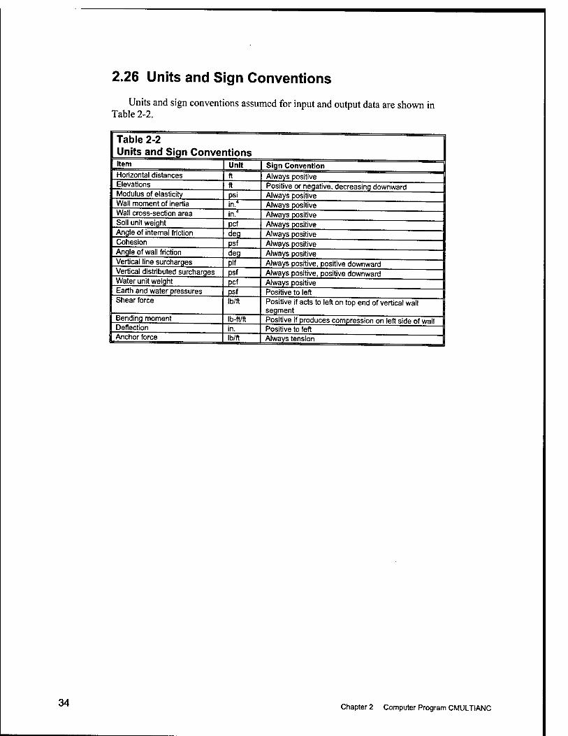
2.26 Units and Sign Conventions
Units and sign conventions assumed for input and output data are shown in Table 2-2.
Table 2-2 Units and Sign Conventions Kern Unit Sign Convention Horizontal distances ft Always positive Elevations ft Positive or negative, decreasing downward Modulus of elasticity psi Always positive Wall moment of inertia in.^ Always positive Wall cross-section area In.' Always positive Soil unit weight pcf Always positive Angle of internal friction deg Always positive Cohesion psf Always positive Angle of wall friction deg Always positive Vertical line surcharges pit Always positive, positive downward Vertical distributed surcharges psf Always positive, positive downward Water unit weight pcf Always positive Earth and water pressures psf Positive to left Shear force lb/ft Positive if acts to left on top end of vertical wall
segment Bending moment Ib-ft/ft Positive if produces compression on left side of wall Deflection in. Positive to left Anchor force lb/ft Always tension
34 Chapter 2 Computer Program CMULTIANC
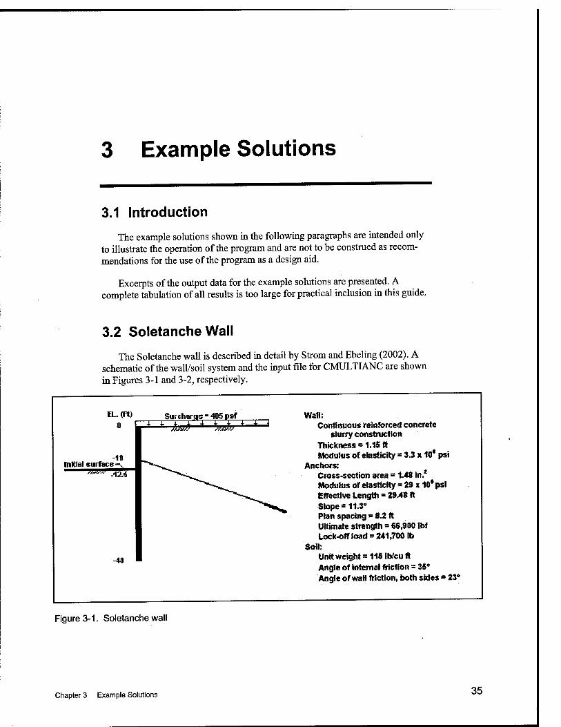
3 Example Solutions
3.1 Introduction
The example solutions shown in the following paragraphs are intended only to illustrate the operation of the program and are not to be construed as recom- mendations for the use of the program as a design aid.
Excerpts of the output data for the example solutions are presented. A complete tabulation of all results is too large for practical inclusion in this guide.
3.2 Soletanche Wall
The Soletanche wall is described in detail by Strom and Ebeling (2002). A schematic of the wall/soil system and the input file for CMULTIANC are shown in Figures 3-1 and 3-2, respectively.
^L. (Ft) Surcharge = 405 pgf
-10 Initial surf ace-v.
-12.S
-40
Wall: Cfmiinuom rettiforced concrete
Thickness s 1.1$ ft Modulus of eftcis^ic% = 3.3 x 10* psi
Ancliors: CrosS'Section area = 1-4B In.* Modulus of elastlcil^ - 2» x 14* psi Iffective Length = 29M ft SkH>e=11.3° Plan spacmg = 8.2 ft UIHmale strength = S6,900 Ibf Lock-off load = 241,700 tb
Soil: Unit weight = IIS Ib/cw ft Angle of hntef nal irictloii = 35« Angle of wall fMctlon, both sides « 23*
Figure 3-1. Soletanche wall
Chapter 3 Example Solutions 35
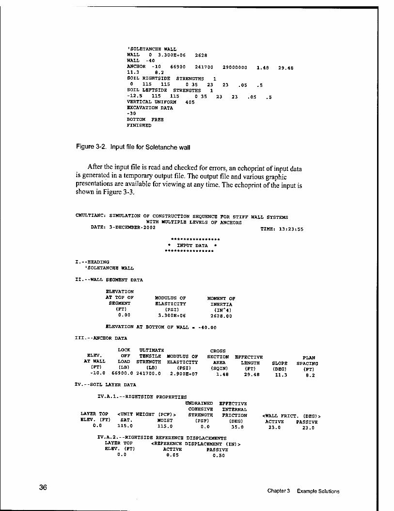
'SOLETANCHE WALL WALL 0 3.300E+06 2628 WALL -40 ANCHOR -10 66900 11.3 8.2 SOIL RIGHTSIDE STRENGTHS 1 0 115 115 0 35 23
SOIL LEFTSIDE STRENGTHS 1 -12.5 115 115 0 35 23 VERTICAL UNIFORM 405 EXCAVATION DATA -30 BOTTOM FREE FINISHED
241700 29000000 1.48 29.48
23 .05 .5
23 .05
Figure 3-2. Input file for Soletanche wall
After the input file is read and checked for errors, an echoprint of input data is generated in a temporary output file. The output file and various graphic presentations are available for viewing at any time. The echoprint of the input is shown in Figure 3-3.
CMULTIANC: SIMULATION OF CONSTRUCTION SEQUENCE FOR STIFF WALL SYSTEMS WITH MULTIPLE LEVELS OF ANCHORS
DATE: 3-DECEMBER-2002 TIME: 13:23:55
* INPUT DATA •
I.--HEADING 'SOLETANCHE WALL
II.--WALL SEGMENT DATA
ELEVATION AT TOP OF SEGMENT
(FT) 0.00
MODULUS OF ELASTICITY
(PSD 3.300E+06
ELEVATION AT BOTTOM OF WALL •
III.--ANCHOR DATA
MOMENT OF INERTIA (IN"4)
2628.00
-40.00
LOCK ULTIMATE ELEV. OFF TENSILE MODULUS OF
AT WALL LOAD STRENGTH ELASTICITY (FT) (LB) (LB) (PSD -10.0 66900.0 241700.0 2.900E+07
IV.--SOIL LAYER DATA
CROSS SECTION EFFECTIVE AREA LENGTH (SQIN) (FT) 1.48 29.48
PLAN SLOPE SPACING (DEG) (FT) 11.3 8.2
IV.A.l.--RIGHTSIDE PROPERTIES UNDRAINED COHESIVE
LAYER TOP <UNIT WEIGHT (PCF) > STRENGTH ELEV. (FT) SAT. MOIST (PSF)
0.0 115.0 115.0 0.0
EFFECTIVE INTERNAL FRICTION
(DEG) 35.0
IV.A.2.--RIGHTSIDE REFERENCE DISPLACEMENTS LAYER TOP <REFERENCE DISPLACEMENT (IN) > ELEV. (FT) ACTIVE PASSIVE
0.0 0.05 0.50
<WALL FRICT. (DEG)> ACTIVE PASSIVE
23.0 23.0
36 Chapter 3 Example Solutions
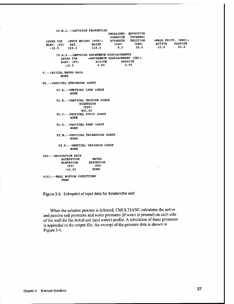
IV.B.l.--LEFTSIDE PROPERTIES UNDRAINED EFFECTIVE COHESIVE INTERNAL
LAYER TOP <UNIT WEIGHT (PCF)> STRENGTH FRICTION <WALL FRICT. (DEG)> ELEV. (FT) SAT. MOIST (PSF) (DEG) ACTIVE PASSIVE
-12.5 115.0 115.0 0.0 35.0 23.0 23.0
IV.A.2.--LEFTSIDE REFERENCE DISPLACEMENTS LAYER TOP <REFERENCE DISPLACEMENT (IN) > ELEV. (FT) ACTIVE PASSIVE
-12.5 0.05 0.50
V.--INITIAL WATER DATA NONE
VI.--VERTICAL SURCHARGE LOADS
VI.A.--VERTICAL LINE LOADS NONE
VLB.--VERTICAL UNIFORM LOADS RIGHTSIDE
(PSF) 405.00
VI.C.--VERTICAL STRIP LOADS NONE
VI.D.--VERTICAL RAMP LOADS NONE
VI.E.--VERTICAL TRIANGULAR LOADS NONE
VI.F.--VERTICAL VARIABLE LOADS NONE
VII.--EXCAVATION DATA EXCAVATION WATER ELEVATION ELEVATION
(FT) (FT) -30.00 NONE
VIII.--WALL BOTTOM CONDITIONS FREE
Figure 3-3. Echoprint of input data for Soletanclie wall
When the solution process is initiated, CMULTIANC calculates the active and passive soil pressures and water pressures (if vi^ater is present) on each side of the wall for the initial soil (and water) profile. A tabulation of these pressures is appended to the output file. An excerpt of the pressure data is shown in Figure 3-4.
Chapters Example Solutions ^'
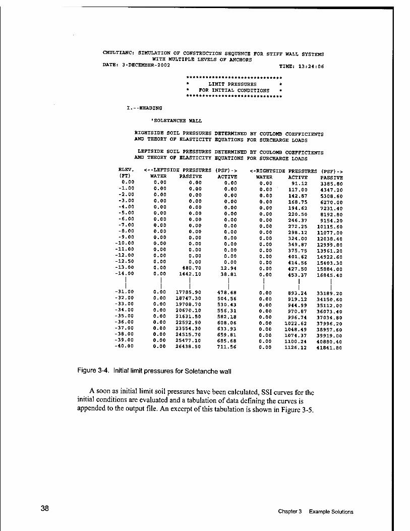
38
CMULTIANC: SIMULATION OF CONSTRUCTION SEQUENCE FOR STIFF WALL SYSTEMS WITH MULTIPLE LEVELS OF ANCHORS
DATE: 3-DECEMBER-2002 TIME: 13:24 :06
****************************** * LIMIT PRESSURES * * FOR INITIAL CONDITIONS * ******************************
I.- -HEADING
•SOLETANCHE WALL
RIGHTSIDE SOIL PRESSURES DETERMINE! BY COULOMB COEFFICIENTS 1 AND THEORY OF ELASTICITY EQUATIONS FOR SURCHARGE LOADS
LEFTSIDE SOIL PRESSURES DETERMINED BY COULOMB COEFFICIENTS 1 AND THEORY OF ELASTICITY EQUATIONS FOR SURCHARGE LOADS
ELEV. <--LEFTSIDE PRESSURES (PSF)-> <-RIUUTSIDE PRESSURES (PSF)-> 1 (FT) WATER PASSIVE ACTIVE WATER ACTIVE PASSIVE 0.00 0.00 0.00 0.00 0.00 91.12 3385.80
-1.00 0.00 0.00 0.00 0.00 117.00 4347.20 -2.00 0.00 0.00 0.00 0.00 142.87 5308.60 -3.00 0.00 0.00 0.00 0.00 168.75 6270.00 -4.00 0.00 0.00 0.00 0.00 194.62 7231.40 -5.00 0.00 0.00 0.00 0.00 220.50 8192.80 -6.00 0.00 0.00 0.00 0.00 246.37 9154.20 -7.00 0.00 0.00 0.00 0.00 272.25 10115.60 -8.00 0.00 0.00 0.00 0.00 298.12 11077.00 -9.00 0.00 0.00 0.00 0.00 324.00 12038.40
-10.00 0.00 0.00 0.00 0.00 349.87 12999.80 -11.00 0.00 0.00 0.00 0.00 375.75 13961.20 -12.00 0.00 0.00 0.00 0.00 401.62 14922.60 -12.50 0.00 0.00 0.00 0.00 414.56 15403.30 -13.00 0.00 480.70 12.94 0.00 427.50 15884.00 -14.00 0.00
1 1442.10 38.81
1 0.00 453.37
1 16845.40
1 -31.00
1 0.00 17785.90
1 478.68 0.00
1 893.24
1 33189.20
-32.00 0.00 18747.30 504.56 0.00 919.12 34150.60 -33.00 0.00 19708.70 530.43 0.00 944.99 35112.00 -34.00 0.00 20670.10 556.31 0.00 970.87 36073.40 -35.00 0.00 21631.50 582.18 0.00 996.74 37034.80 -36.00 0.00 22592.90 608.06 0.00 1022.62 37996.20 -37.00 0.00 23554.30 633.93 0.00 1048.49 38957.60 -38.00 0.00 24515.70 659.81 0.00 1074.37 39919.00 -39.00 0.00 25477.10 685.68 0.00 1100.24 40880.40 -40.00 0.00 26438.50 711.56 0.00 1126.12 41841.80
Figure 3-4. Initial limit pressures for Soletanche wail
A soon as initial limit soil pressures have been calculated, SSI curves for the initial conditions are evaluated and a tabulation of data defining the curves is appended to the output file. An excerpt of this tabulation is shown in Figure 3-5.
Chapter 3 Example Solutions
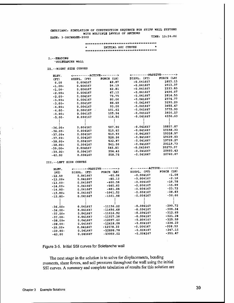
CMULTIANC: SIMULATION OF CONSTRUCTION SEQUENCE FOR STIFF WALL SYSTEMS WITH MULTIPLE LEVELS OF ANCHORS
DATE: 3-DECEMBER-2002 TIME: 13:24:06
*************************************** * INITIAL SSI CURVES * ***************************************
I.--HEADING •SOLETANCHE WALL
II.--RIGHT SIDE CURVES
< ACTIVE < PASS IVE > ELEV. (FT) DISPL. (FT) FORCE (LB) DISPL. (FT) FORCE (LB)
0.00 0.004167 49.87 -0.041667 1853.13
-1.00+ 0.004167 54.19 -0.041667 2013.37
-1.00- 0.004167 62.81 -0.041667 2333.83
-2.00+ 0.004167 67.12 -0.041667 2494.07
-2.00- 0.004167 75.75 -0.041667 2814.53
-3.00+ 0.004167 80.06 -0.041667 2974.77
-3.00- 0.004167 88.69 -0.041667 3295.23
-4.00+ 0.004167 93.00 -0.041667 3455.47
-4.00- 0.004167 101.62 -0.041667 3775.93
-5.00+ 0.004167 105.94 -0.041667 3936.17
-5.00- 1
0.004167 114.56 -0.041667
1 4256.63
1 -36.00+ 0.004167 507.00
1 -0.041667 18837.87
-36.00- 0.004167 515.62 -0.041667 19158.33
-37.00+ 0.004167 519.93 -0.041667 19318.57
-37.00- 0.004167 528.56 -0.041667 19639.03
-38.00+ 0.004167 532.87 -0.041667 19799.27
-38.00- 0.004167 541.50 -0.041667 20119.73
-39.00+ 0.004167 545.81 -0.041667 20279.97
-39.00- 0.004167 554.43 -0.041667 20600.43
-40.00 0.004167 558.75 -0.041667 20760.67
III.--LEFT SIDE CURVES
ELEV. < PASSIVE > < AUli VJS ^
(FT) DISPL. (FT) FORCE (LB) DISPL. (FT) FORCE (LB)
12.50 0.041667 -40.06 -0.004167 -1.08
13.00+ 0.041667 -80.12 -0.004167 -2.16
13.00- 0.041667 -400.58 -0.004167 -10.78
14.00+ 0.041667 -560.82 -0.004167 -15.09
14.00- 0.041667 -881.28 -0.004167 -23.72
15.00+ 0.041667 -1041.52 -0.004167 -28.03
15.00- 1
0.041667 -1361.98
1 -0.004167
1 -36.66
1 36.00+ 0.041667
1 -11136.22
1 -0.004167 -299.72
36.00- 0.041667 -11456.68 -0.004167 -308.34
37.00+ 0.041667 -11616.92 -0.004167 -312.65
37.00- 0.041667 -11937.38 -0.004167 -321.28
38.00+ 0.041667 -12097.62 -0.004167 -325.59
38.00- 0.041667 -12418.08 -0.004167 -334.22
39.00+ 0.041667 -12578.32 -0.004167 -338.53
-39.00- 0.041667 -12898.78 -0.004167 -347.15
■40.00 0.041667 -13059.02 -0.004167 -351.47
Figure 3-5. Initial SSI curves for Soletanche wail
The next stage in the solution is to solve for displacements, bending moments, shear forces, and soil pressures throughout the wall using the initial SSI curves. A summary and complete tabulation of results for this solution are
Chapter 3 Example Solutions 39
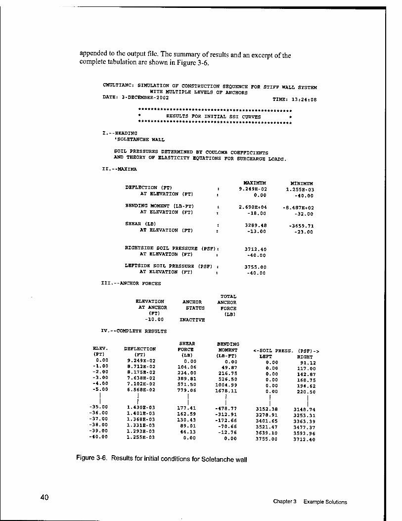
appended to the output file. The summary of results and an excerpt of the complete tabulation are shown in Figure 3-6.
CMULTIANC: SIMULATION OF CONSTRUCTION SEQUENCE FOR STIFF WALL SYSTEM WITH MULTIPLE LEVELS OF ANCHORS
DATE: 3-DECEMBER-2002 TIME: 13:24:08
* RESULTS FOR INITIAL SSI CURVES *
I. - -HEADING 'SOLETANCHE WALL
SOIL PRESSURES DETERMINED BY COULOMB COEFFICIENTS AND THEORY OF ELASTICITY EQUATIONS FOR SURCHARGE LOADS.
II.--MAXIMA
DEFLECTION (FT) AT ELEVATION (FT)
BENDING MOMENT (LB-FT) AT ELEVATION (FT)
SHEAR (LB) AT ELEVATION (FT)
RIGHTSIDE SOIL PRESSURE (PSF) AT ELEVATION (FT) i
LEFTSIDE SOIL PRESSURE (PSF) AT ELEVATION (FT) ;
III.--ANCHOR FORCES
MAXIMUM BJINIMUM 9.249E-02 1.255E-03
0.00 -40.00
2.690E+04 -8.487E+02 -18.00 -32.00
3289.48 -3659.71 -13.00 -23.00
3712.40 -40.00
3755.00 -40.00
ELEVATION AT ANCHOR
(FT) -10.00
IV.--COMPLETE RESULTS
ANCHOR STATUS
INACTIVE
TOTAL ANCHOR FORCE (LB)
ELEV. DEFLECTION (FT) (FT) 0.00 9.249E-02
-1.00 8.712E-02 -2.00 8.175E-02 -3.00 7.638E-02 -4.00 7.102E-02 -5.00
1 6.568E-02
1 1
35.00 1
1.430E-03 36.00 1.401E-03 37.00 1.368E-03 38.00 1.331E-03 39.00 1.293E-03 40.00 1.255E-03
SHEAR FORCE (LB) 0 .00
104 .06 234 .00 389 81 571 50 779 06
177 41 162 59 130 43 89 01 44 13 0 00
BENDING MOMENT (LB-FT)
0.00 49.87 216.75 526.50
1004.99 1678.11
-478.77 -312.91 -172.66 -70.66 -12.76
0.00
<-SOIL PRESS. (PSF)-> LEFT
0 0 0 0 0 0
00 00 00 00 00 00
3152.38 3278.91 3401.65 3521.47 3639.10 3755.00
RIGHT 91.12
117.00 142.87 168.75 194.62 220.50
3148.74 3253.31 3363.39 3477.37 3593.96 3712.40
Figure 3-6. Results for initial conditions for Soletanche wall
40 Chapter 3 Example Solutions
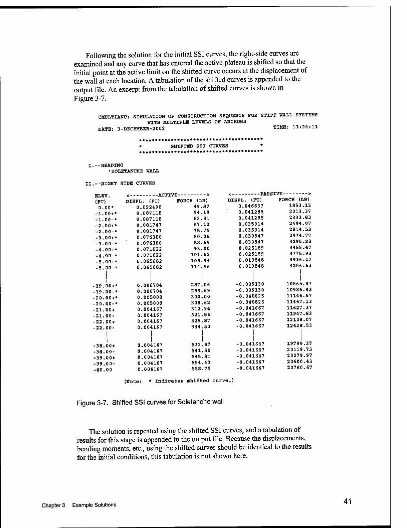
Following the solution for the initial SSI curves, the right-side curves are examined and any curve that has entered the active plateau is shifted so that the initial point at the active limit on the shifted curve occurs at the displacement of the wall at each location. A tabulation of the shifted curves is appended to the output file. An excerpt fi-om the tabulation of shifted curves is shovm in Figure 3-7.
CMULTIANC: SIMULATION OF CONSTRUCTION SEQUENCE FOR STIFF WALL SYSTEMS WITH MULTIPLE LEVELS OF ANCHORS
DATE: 3-DECEMBER-2002 TIME: 13:24:11
*************************************** * SHIFTED SSI CURVES * ***************************************
--HEADING ■SOLETANCHE WALL
--RIGHT SIDE CURVES
<- ACTIVE <- PASS IVE > ELEV. (FT) DISPL. (FT) FORCE (LB) DISPL. (FT) FORCE (LB)
0.00* 0.092490 49.87 0.046657 1853.13
-1.00+* 0.087118 54.19 0.041285 2013.37
-1.00-* 0.087118 62.81 0.041285 2333.83
-2.00+* 0.081747 67.12 0.035914 2494.07
-2.00-* 0.081747 75.75 0.035914 2814.53
-3.00+* 0.076380 80.06 0.030547 2974.77
-3.00-* 0.076380 88.69 0.030547 3295.23
-4.00+* 0.071022 93.00 0.025189 3455.47
-4.00-* 0.071022 101.62 0.025189 3775.93
-5.00+* 0.065682 105.94 0.019848 3936.17
-5.00-* 1
0.065682 1
114.56
1 0.019848 4256.63
i -19.00+*
1 0.006704
1 287.06 -0.039130 10665.97
-19.00-* 0.006704 295.69 -0.039130 10986.43
-20.00+* 0.005008 300.00 -0.040825 11146.67
-20.00-* 0.005008 308.62 -0.040825 11467.13
-21.00+ 0.004167 312.94 -0.041667 11627.37
-21.00- 0.004167 321.56 -0.041667 11947.83
-22.00+ 0.004167 325.87 -0.041667 12108.07
-22.00- 1
0.004167 1
334.50 -0.041667
1 12428.53
1 1
■38.00+ 1
0.004167 532.87 1
-0.041667 1
19799.27
-38.00- 0.004167 541.50 -0.041667 20119.73
-39.00+ 0.004167 545.81 -0.041667 20279.97
-39.00- 0.004167 554.43 -0.041667 20600.43
-40.00 0.004167 558.75 -0.041667 20760.67
(Note: * Indicates shifted curve.)
Figure 3-7. Shifted SSI curves for Soletanche wall
The solution is repeated using the shifted SSI curves, and a tabulation of results for this stage is appended to the output file. Because the displacements, bending moments, etc., using the shifted curves should be identical to the results for the initial conditions, this tabulation is not shovm here.
Chapter 3 Example Solutions 41
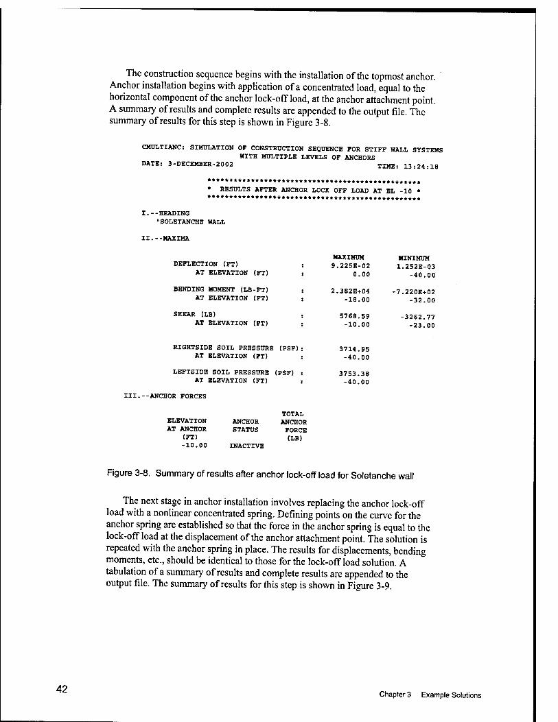
The construction sequence begins with the installation of the topmost anchor. Anchor installation begins with application of a concentrated load, equal to the horizontal component of the anchor lock-offload, at the anchor attachment point. A summary of results and complete results are appended to the output file. The summary of results for this step is shown in Figure 3-8.
CMULTIANC: SIMULATION OF CONSTRUCTION SEQUENCE FOR STIFF WALL SYSTEMS WITH MULTIPLE LEVELS OF ANCHORS
DATE: 3-DECEMBER-2002 TIME: 13:24:18
* RESULTS AFTER ANCHOR LOCK OFF LOAD AT EL -10 *
I.--HEADING •SOLETANCHE WALL
II.--MAXIMA
DEFLECTION (FT) AT ELEVATION (FT)
BENDING MOMENT (LB-FT) AT ELEVATION (FT)
SHEAR (LB) AT ELEVATION (FT)
MAXIMUM 9.225E-02
0.00
2.382E+04 -18.00
5768.59 -10.00
MINIMUM 1.252E-03
-40.00
-7.220E+02 -32.00
-3262.77 -23.00
RIGHTSIDE SOIL PRESSURE (PSF) AT ELEVATION (FT)
LEFTSIDE SOIL PRESSURE (PSF) AT ELEVATION (FT)
III.--ANCHOR FORCES
3714.95 -40.00
3753.38 -40.00
ELEVATION AT ANCHOR
(FT) -10.00
TOTAL ANCHOR ANCHOR STATUS FORCE
(LB) INACTIVE
Figure 3-8. Summary of results after anchor lock-off load for Soletanche wall
The next stage in anchor installation involves replacing the anchor lock-off load with a nonlinear concentrated spring. Defining points on the curve for the anchor spring are established so that the force in the anchor spring is equal to the lock-offload at the displacement of the anchor attachment point. The solution is repeated with the anchor spring in place. The results for displacements, bending moments, etc., should be identical to those for the lock-offload solution. A tabulation of a summary of results and complete results are appended to the output file. The summary of results for this step is shown in Figure 3-9.
42 Chapter 3 Example Solutions
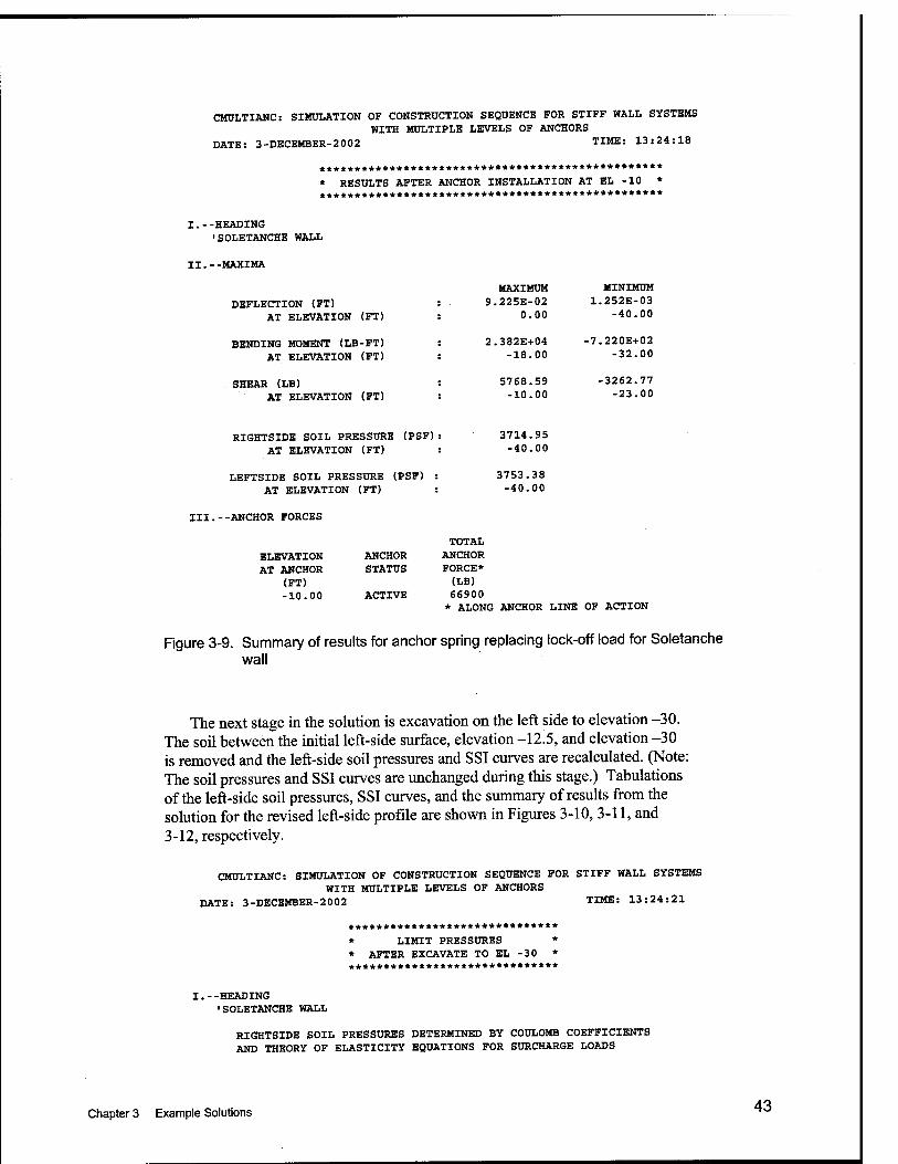
CMULTIANC: SIMULATION OF CONSTRUCTION SEQUENCE FOR STIFF WALL SYSTEMS WITH MULTIPLE LEVELS OF ANCHORS
DATE: 3-DECEMBER-2002 TIME: 13:24:18
************************************************* * RESULTS AFTER ANCHOR INSTALLATION AT EL -10 * *************************************************
I.--HEADING 'SOLETANCHE WALL
II.--MAXIMA
MAXIMUM MINIMUM DEFLECTION (FT) : 9.225E-02 1.252E-03
AT ELEVATION (FT) : 0.00 -40.00
BENDING MOMENT (LB-FT) : 2.382E+04 -7.220E+02 AT ELEVATION (FT) : -18.00 -32.00
SHEAR (LB). : 5768.59 -3262.77 AT ELEVATION (FT) : -10.00 -23.00
RIGHTSIDE SOIL PRESSURE (PSF): 3714.95 AT ELEVATION (FT) : -40.00
LEFTSIDE SOIL PRESSURE (PSF) : 3753.38 AT ELEVATION (FT) : -40.00
III.--ANCHOR FORCES
TOTAL ELEVATION ANCHOR ANCHOR AT ANCHOR STATUS FORCE*
(FT) (LB) -10.00 ACTIVE 66900
* ALONG ANCHOR LINE OF ACTION
Figure 3-9. Summary of results for anchor spring replacing lock-off load for Soletanche wall
The next stage in the solution is excavation on the left side to elevation -30. The soil between the initial left-side surface, elevation -12.5, and elevation -30 is removed and the left-side soil pressures and SSI curves are recalculated. (Note: The soil pressures and SSI curves are unchanged during this stage.) Tabulations of the left-side soil pressures, SSI curves, and the summary of results from the solution for the revised left-side profile are shovra in Figures 3-10, 3-11, and 3-12, respectively.
CMULTIANC: SIMULATION OF CONSTRUCTION SEQUENCE FOR STIFF WALL SYSTEMS WITH MULTIPLE LEVELS OF ANCHORS
DATE: 3-DECEMBER-2002 TIME: 13:24:21
****************************** * LIMIT PRESSURES * * AFTER EXCAVATE TO EL -30 * ******************************
I. - -HEADING •SOLETANCHE WALL
RIGHTSIDE SOIL PRESSURES DETERMINED BY COULOMB COEFFICIENTS AND THEORY OF ELASTICITY EQUATIONS FOR SURCHARGE LOADS
Chapter 3 Example Solutions 43
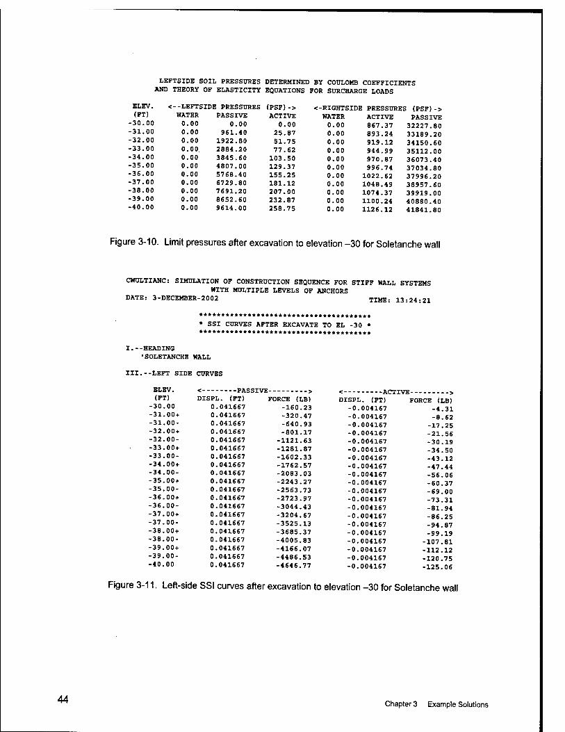
LEFTSIDE SOIL PRESSURES DETERMINED BY COULOMB COEFFICIENTS AND THEORY OF ELASTICITY EQUATIONS FOR SURCHARGE LOADS
ELEV. <-.LEFTSIDE PRESSURES (PSF)-> <-RIGHTSIDE PRESSURES (PSF)-> (FT) WATER PASSIVE ACTIVE WATER ACTIVE PASSIVE 30.00 0.00 0.00 0.00 0.00 867.37 32227.80 31.00 0.00 961.40 25.87 0.00 893.24 33189.20 32.00 0.00 1922.80 51.75 0.00 919.12 34150.60 33.00 0.00 2884.20 77.62 0.00 944.99 35112.00 34.00 0.00 3845.60 103.50 0.00 970.87 36073.40 35.00 0.00 4807.00 129.37 0.00 996.74 37034.80 36.00 0.00 5768.40 155.25 0.00 1022.62 37996.20 37.00 0.00 6729.80 181.12 0.00 1048.49 38957.60 38.00 0.00 7691.20 207.00 0.00 1074.37 39919.00 39.00 0.00 8652.60 232.87 0.00 1100.24 40880.40 40.00 0.00 9614.00 258.75 0.00 1126.12 41841.80
Figure 3-10. Limit pressures after excavation to elevation -30 for Soletanche wall
CMULTIANC: SIMULATION OF CONSTRUCTION SEQUENCE FOR STIFF WALL SYSTEMS WITH MULTIPLE LEVELS OF ANCHORS
DATE: 3-DECEMBER-2002 TIME: 13:24:21
* SSI CURVES AFTER EXCAVATE TO EL -30 * ***************************************
I.--HEADING ■SOLETANCHE WALL
III.--LEFT SIDE CURVES
ELEV. < PASSIVE - — — —-» — __^ ^- — — — — — — — - ZkPTTVT?
(FT) DISPL. (FT) FORCE (LB) ^ — — — — — — — AK- i. X V ri
DISPL. (FT) — --> FORCE (LB)
30.00 0.041667 -160.23 -0.004167 -4.31 31.00+ 0.041667 -320.47 -0.004167 -8.62 31.00- 0.041667 -640.93 -0.004167 -17.25 32.00+ 0.041667 -801.17 -0.004167 -21.56 32.00- 0.041667 -1121.63 -0.004167 -30.19 33.00+ 0.041667 -1281.87 -0.004167 -34.50 33.00- 0.041667 -1602.33 -0.004167 -43.12 34.00+ 0.041667 -1762.57 -0.004167 -47.44 34.00- 0.041667 -2083.03 -0.004167 -56.06 35.00+ 0.041667 -2243.27 -0.004167 -60.37 35.00- 0.041667 -2563.73 -0.004167 -69.00 36.00+ 0.041667 -2723.97 -0.004167 -73.31 36.00- 0.041667 -3044.43 -0.004167 -81.94 37.00+ 0.041667 -3204.67 -0.004167 -86.25 37.00- 0.041667 -3525.13 -0.004167 -94.87 38.00+ 0.041667 -3685.37 -0.004167 -99.19 38.00- 0.041667 -4005.83 -0.004167 -107.81 39.00+ 0.041667 -4166.07 -0.004167 -112.12 39.00- 0.041667 -4486.53 -0.004167 -120.75 40.00 0.041667 -4646.77 -0.004167 -125.06
Figure 3-11. Left-side SSI curves after excavation to elevation -30 for Soletanche wall
44 Chapter 3 Example Solutions
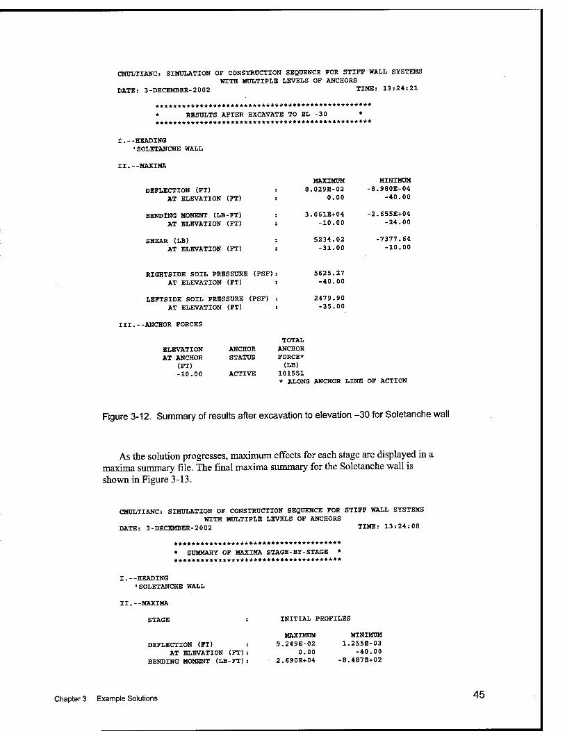
CMULTIANC: SIMULATION OF CONSTRUCTION SEQUENCE FOR STIFF WALL SYSTEMS WITH MULTIPLE LEVELS OF ANCHORS
DATE: 3-DECEMBER-2002 TIME: 13:24:21
************************************************* * RESULTS AFTER EXCAVATE TO EL -30 * *************************************************
I.--HEADING 'SOLETANCHE WALL
II.--MAXIMA
DEFLECTION (FT) AT ELEVATION (FT)
BENDING MOMENT (LB-FT) AT ELEVATION (FT)
SHEAR (LB) AT ELEVATION (FT)
MAXIMUM 8.029E-02
0.00
3.061E+04 -10.00
5234.02 -31.00
MINIMUM -8.980E-04
-40.00
-2.655E+04 -24.00
-7377.64 -10.00
RIGHTSIDE SOIL PRESSURE (PSF); AT ELEVATION (FT)
5625.27 -40.00
LEFTSIDE SOIL PRESSURE (PSF) AT ELEVATION (FT)
2479.90 -35.00
III.--ANCHOR FORCES
TOTAL ELEVATION ANCHOR ANCHOR AT ANCHOR STATUS FORCE*
(FT) (LB) -10.00 ACTIVE 101551
* ALONG ANCHOR LINE OF ACTION
Figure 3-12. Summary of results after excavation to elevation -30 for Soletanche wall
As the solution progresses, maximum effects for each stage are displayed in a maxima summary file. The final maxima summary for the Soletanche wall is shovra in Figure 3-13.
CMULTIANC: SIMULATION OF CONSTRUCTION SEQUENCE FOR STIFF WALL SYSTEMS WITH MULTIPLE LEVELS OF ANCHORS
DATE: 3-DECEMBER-2002 TIME: 13:24:08
************************************** * SUMMARY OF MAXIMA STAGE-BY-STAGE * **************************************
I. - -HEADING 'SOLETANCHE WALL
II.--MAXIMA
STAGE INITIAL PROFILES
DEFLECTION (FT) AT ELEVATION (FT)
BENDING MOMENT (LB-FT)
MAXIMUM 9.249E-02
0.00 2.690E+04
MINIMUM 1.255E-03
-40.00 -8.487E+02
Chapter 3 Example Solutions 45
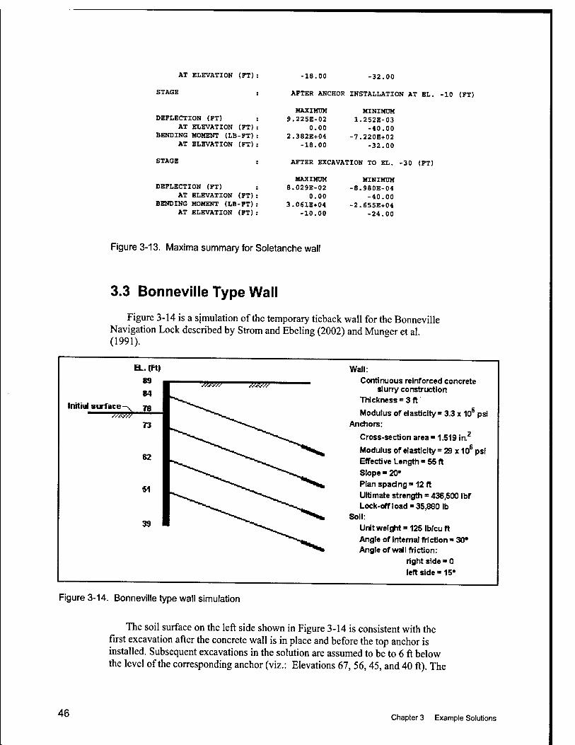
AT ELEVATION (FT) : -18.00 -32.00
STAGE : AFTER ANCHOR INSTALLATION AT EL
MAXIMUM MINIMUM DEFLECTION (FT) 9.225E-02 1.252E-03
AT ELEVATION (FT) 0.00 -40.00 BENDING MOMENT (LB-FT) 2.382E+04 -7.220E+02
AT ELEVATION (FT) -18.00 -32.00
STAGE AFTER EXCAVATION TO EL. - 30 (FT
MAXIMUM MINIMUM DEFLECTION (FT) 8.029E-02 -8.980E-04
AT ELEVATION (FT) 0.00 -40.00 BENDING MOMENT (LB-FT) 3.061E+04 -2.655E+04
AT ELEVATION (FT) -10.00 -24.00
-10 (FT)
Figure 3-13. Maxima summary for Soletanche wall
3.3 Bonneville Type Wall
Figure 3-14 is a simulation of the temporary tieback wall for the Bonneville Navigation Lock described by Strom and Ebeling (2002) and Munger et al (1991).
Irritial surface-^ 77?^
EL.(R)
89
84
78
73
62
SI
39
"TZlTTr -m^TT
Wall: Continuous reinforced concrete
slurry construction Thickness =3 ft
Modulus of elasticity = 3.3 x 10^ psi Andiors:
Cross-section area= 1.519 ia^
Modulus of elasticity=29 x 10^ psi EfTective Lengtti = 55 ft Slope " 20» Plan spacing »12 ft Ultimate strengtii = 436,500 Ibf Lock-offload-35,880 lb
Soil: Unitweiglit=125lb/cuft Angle of internal friction = 30* Angle of wall friction:
rlgtit side =» 0 left side -15*
Figure 3-14. Bonneville type wail simulation
The soil surface on the left side shown in Figure 3-14 is consistent with the first excavation after the concrete wall is in place and before the top anchor is installed. Subsequent excavations in the solution are assumed to be to 6 ft below the level of the corresponding anchor (viz.: Elevations 67, 56, 45, and 40 ft). The
46 Chapter 3 Example Solutions
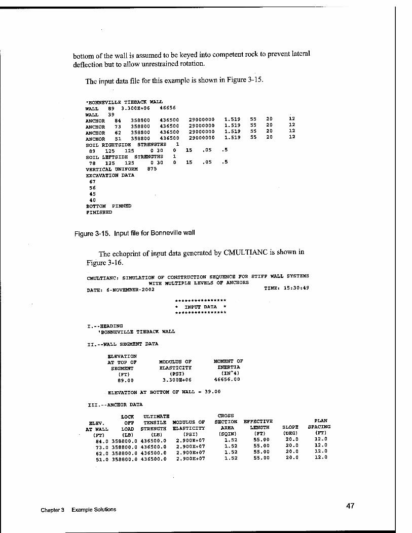
bottom of the wall is assumed to be keyed into competent rock to prevent lateral deflection but to allow unrestrained rotation.
The input data file for this example is shown in Figure 3-15.
■BONNEVILLE TIEBACK WALL WALL 89 3.300E+06 46656 WALL 39 ANCHOR 84 358800 436500 ANCHOR 73 358800 436500 ANCHOR 62 358800 436500 ANCHOR 51 358800 436500
29000000 29000000 29000000 29000000
1 1 1 1
519 519 519 519
55 55 55 55
20 20 20 20
12 12 12 12
SOIL RIGHTSIDE STRENGTHS 1 89 125 125 0 30 0 15 .05 .5
SOIL LEFTSIDE STRENGTHS 1 78 125 125 0 30 0 15 .05 .5
VERTICAL UNIFORM 875 EXCAVATION DATA 67 56 45 40
BOTTOM PINNED FINISHED
Figure 3-15. Input file for Bonnevilie wall
The echoprint of input data generated by CMULTIANC is shown in Figure 3-16.
CMULTIANC: SIMULATION OF CONSTRUCTION SEQUENCE FOR STIFF WALL SYSTEMS WITH MULTIPLE LEVELS OF ANCHORS
DATE: 6-NOVEMBER-2 002 TIME: 15:30:49
**************** * INPUT DATA * ****************
I.--HEADING •BONNEVILLE TIEBACK WALL
II.--WALL SEGMENT DATA
ELEVATION AT TOP OF MODULUS OF MOMENT OF SEGMENT ELASTICITY INERTIA
(FT) (PSD (IN*4)
89.00 3. 300E+06 46656.00
ELEVATION AT BOTTOM OF WALL =39 .00
III.--ANCHOR DATA
LOCK ULTIMATE CROSS
ELEV. OFF TENSILE MODULUS OF SECTION EFFECTIVE PLAN
AT WALL LOAD STRENGTH ELASTICITY AREA LENGTH SLOPE SPACING
(FT) (LB) (LB) (PSD (SQIN) (FT) (DEG) (FT)
84.0 358800.0 436500.0 2.900E+07 1.52 55.00 20.0 12.0
73.0 358800.0 436500.0 2.900E+07 1.52 55.00 20.0 12.0
62.0 358800.0 436500.0 2.900E+07 1.52 55.00 20.0 12.0
51.0 358800.0 436500.0 2.900E+07 1.52 55.00 20.0 12.0
Chapter 3 Example Solutions 47
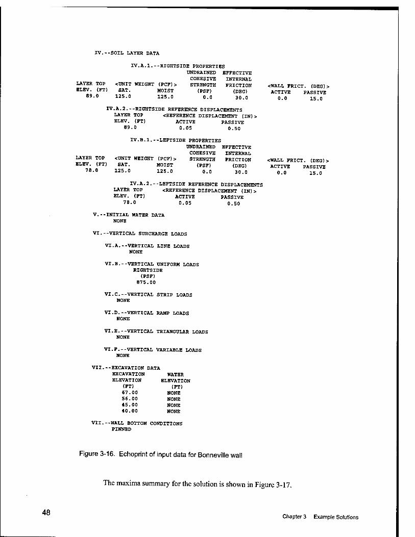
IV.—SOIL LAYER DATA
IV.A.1.--RIGHTSIDE PROPERTIES DNDRAINED EFFECTIVE COHESIVE INTERNAL
LAYER TOP <DNIT WEIGHT (PCF)> STRENGTH FRICTION <WALL FRICT. (DEG)> ELEV. (FT) SAT. MOIST (PSF) (DEG) ACTIVE PASSIVE
89-0 125.0 125.0 0.0 30.0 0.0 15.0
IV.A.2.--RIGHTSIDE REFERENCE DISPLACEMENTS LAYER TOP <REFERENCE DISPLACEMENT (IN) > ELEV. (FT) ACTIVE PASSIVE
89.0 0.05 0.50
IV.B.l.--LEFTSIDE PROPERTIES DNDRAINED EFFECTIVE COHESIVE INTERNAL
LAYER TOP <DNIT WEIGHT (PCF) > STRENGTH FRICTION <WALL FRICT. (DEG) > ELEV. (FT) SAT. MOIST (PSF) (DEG) ACTIVE PASSIVE
'S-O 125.0 125.0 0.0 30.0 0.0 15.0
IV.A.2.--LEFTSIDE REFERENCE DISPLACEMENTS LAYER TOP <REFERENCE DISPLACEMENT (IN) > ELEV. (FT) ACTIVE PASSIVE
78.0 0.05 0.50
v.--INITIAL WATER DATA NONE
VI.--VERTICAL SURCHARGE LOADS
VI.A.--VERTICAL LINE LOADS NONE
VI.B.--VERTICAL UNIFORM LOADS RIGHTS IDE
(PSF) 875.00
VI.C.--VERTICAL STRIP LOADS NONE
VI.D.--VERTICAL RAMP LOADS NONE
VI.E.--VERTICAL TRIANGULAR LOADS NONE
VI.F.--VERTICAL VARIABLE LOADS NONE
VII.--EXCAVATION DATA EXCAVATION WATER ELEVATION ELEVATION
(FT) (FT) 67.00 NONE 56.00 NONE 45.00 NONE 40.00 NONE
VII.--WALL BOTTOM CONDITIONS PINNED
Figure 3-16. Echoprint of input data for Bonneville wall
The maxima summary for the solution is shown in Figure 3-17.
48 Chapter 3 Example Solutions
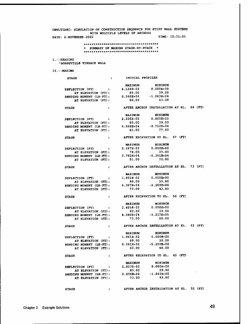
CMULTIANC: SIMULATION OF CONSTRUCTION SEQUENCE FOR STIFF WALL SYSTEMS WITH MULTIPLE LEVELS OF ANCHORS
DATE: 6-NOVEMBER-2002 TIME: 15:31:00
************************************** * SUMMARY OF MAXIMA STA6E-BY-STA6E * **************************************
I.--HEADING ■BONNEVILLE TIEBACK WALL
II.--MAXIMA
STAGE INITIAL PROFILES
DEFLECTION (FT) AT ELEVATION (FT)
BENDING MOMENT (LB-FT) AT ELEVATION (FT)
MAXIMUM 4.136E-02
89.00 8.366E+04
66.00
MINIMUM O.OOOE-fOO
39.00 -1.063E+04
43.00
STAGE AFTER ANCHOR INSTALLATION AT EL. 84 (FT)
DEFLECTION (FT) AT ELEVATION (FT)
BENDING MOMENT (LB-FT) AT ELEVATION (FT)
MAXIMUM 2.225E-02
89.00 4.588E+04
61.00
MINIMUM O.OOOE+00
39.00 -2.712E+04
77.00
STAGE AFTER EXCAVATION TO EL. 67 (FT)
DEFLECTION (FT) AT ELEVATION (FT)
BENDING MOMENT (LB-FT) AT ELEVATION (FT)
MAXIMUM 2.167E-02
78.00 2.782E+04
51.00
MINIMUM O.OOOE+00
39.00 -6.361E+04
71.00
STAGE AFTER ANCHOR INSTALLATION AT EL. 73 (FT)
DEFLECTION (FT) AT ELEVATION (FT)
BENDING MOMENT (LB-FT) AT ELEVATION (FT)
MAXIMUM .901E-02
89.00 .367E+04
73.00
MINIMUM .OOOE+00
39.00 .269E+04
43.00
STAGE AFTER EXCAVATION TO EL. 56 (FT)
DEFLECTION (FT) AT ELEVATION (FT)
BENDING MOMENT (LB-FT) AT ELEVATION (FT)
MAXIMUM .401E-02
62.00 .089E+04
73.00
MINIMUM O.OOOE+00
39.00 -1.217E+05
58.00
STAGE AFTER ANCHOR INSTALLATION AT EL. 62 (FT)
DEFLECTION (FT) AT ELEVATION (FT)
BENDING MOMENT (LB-FT) AT ELEVATION (FT)
MAXIMUM .961E-02
89.00 .261E+04
62.00
MINIMUM O.OOOE+00
39.00 -5.209E+04
48.00
STAGE AFTER EXCAVATION TO EL. 45 (FT)
DEFLECTION (FT) AT ELEVATION (FT)
BENDING MOMENT (LB-FT) AT ELEVATION (FT)
MAXIMUM 1.817E-02
89.00 6.104E+04
73.00
MINIMUM O.OOOE+00
39.00 -1.043E+05
49.00
STAGE AFTER ANCHOR INSTALLATION AT EL. 51 (FT)
Chapter 3 Example Solutions 49
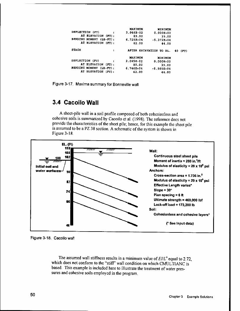
MAXIMUM MINIMUM DEFLECTION (FT) 2.046E-02 O.OOOE+00
AT ELEVATION (FT) 89.00 39.00 BENDING MOMENT (LB-FT) 6.725E+04 -5.372E+04
AT ELEVATION (FT) 62.00 44.00
STAGE AFTER EXCAVATION TO EL.
MAXIMUM MINIMUM DEFLECTION (FT) 2.045E-02 O.OOOE+00
AT ELEVATION (FT) 89.00 39.00 BENDING MOMENT (LB-FT) 6.746E+04 -5.565E+04
AT ELEVATION (FT) 62.00 44.00
40 (FT)
Figure 3-17. Maxima summary for Bonneville wall
3.4 CacoiloWall
A sheet-pile wall in a soil profile composed of both cohesionless and cohesive soils is summarized by Cacoilo et al. (1998). The reference does not provide the characteristics of the sheet pile; hence, for this example the sheet pile is assumed to be a PZ 38 section. A schematic of the system is shown in Figure 3-18.
▼ 100
EL.(R) 110 106 102
-^ ?W,
Initial soil and water surfaces-' 99 7
46
^?!!9?, ^^A>V Wall: Continuous steel sheet pile Moment of inertia = 280 in.^/ft Modulus of elasticity = 29 x 10* psi
Anchors: Cross-section area = 1.736 in.' Modulus of elasticity = 29 x 10* psi Effective Length varies* Slope = 30° Plan spacing = 6 ft Ultimate strength = 469,000 Ibf Lock-off load = 173,200 lb
Soil:
Cohesionless and cohesive layers*
(* See input data)
Figure 3-18. Cacoilo wail
The assumed wall stiffness results in a minimum value of £■///." equal to 2.72, which does not conform to the "stiff wall condition on which CMULTIANC is ' based. This example is included here to illustrate the treatment of water pres- sures and cohesive soils employed in the program.
50 Chapter 3 Example Solutions
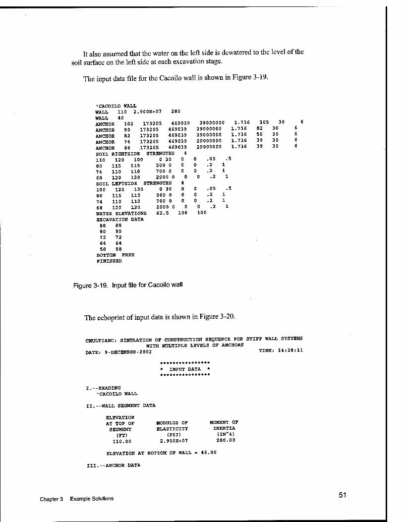
It also assumed that the water on the left side is dewatered to the level of the soil surface on the left side at each excavation stage.
The input data file for the Cacoilo wall is shown in Figure 3-19.
•CACOILO WALL WALL 110 2.900E+07 280 WALL 46 ANCHOR 102 173205 469039 29000000 1.736 105 30 6
ANCHOR 90 173205 469039 29000000 1.736 82 30 6
ANCHOR 82 173205 469039 29000000 1.736 56 30 6
ANCHOR 74 173205 469039 29000000 1.736 39 30 6
ANCHOR 66 173205 469039 29000000 1.736 39 30 6
SOIL RIGHTSIDE STRENGTHS 4 110 120 100 0 30 0 0 .05 .5
80 115 115 300 0 0 0 .2 1
74 110 110 700 0 0 0 .2 1
68 120 120 2000 0 0 0 .2 1
SOIL LEFTSIDE STRENGTHS 4 100 120 100 0 30 0 0 .05 .5
80 115 115 300 0 0 0 .2 1
74 110 110 700 0 0 0 .2 1
68 120 120 2000 0 0 0.2 1
WATER ELEVATIONS 62.5 106 100
•EXCAVATION DATA 88 88 80 80 72 72 64 64 58 58
BOTTOM FREE FINISHED
Figure 3-19. Input file for Cacoilo wall
The echoprint of input data is shown in Figure 3-20.
CMULTIANC: SIMULATION OF CONSTRttCTION SEQUENCE FOR STIFF WALL SYSTEMS WITH MULTIPLE CEVELS OF ANCHORS
DATE: 9-DECEMBER-2002 TIME: 14:28:11
**************** * INPUT DATA *
I. - -HEADING 'CACOILO WALL
II.--WALL SEGMENT DATA
ELEVATION AT TOP OF MODULUS OF MOMENT OF
SEGMENT ELASTICITY INERTIA
(FT) (PSD (IN"4)
110.00 2.900E+07 280.00
ELEVATION AT BOTTOM OF WALL = 46.00
III.--ANCHOR DATA
Chapter 3 Example Solutions 51
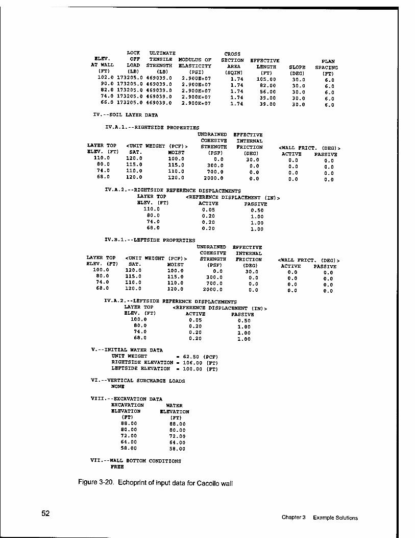
LOCK ULTIMATE CROSS ELEV. OFF TENSILE MODULUS OF SECTION EFFECTIVE PLAN
AT WALL LOAD STRENGTH ELASTICITY AREA LENC3TH SLOPE SPACING (FT) (LB) (LB) (PSI) (SQIN) (FT) (DEG) (FT) 102.0 173205.0 469039.0 2.900E+07 1.74 105.00 30.0 6.0 90.0 173205.0 469039.0 2.900E+07 1.74 82.00 30.0 6.0 82.0 173205.0 469039.0 2.900E+07 1.74 56.00 30.0 6.0 74.0 173205.0 469039.0 2.900E+07 1.74 39.00 30.0 6.0 66.0 173205.0 469039.0 2.900E+07 1.74 39.00 30.0 6.0
IV.--SOIL LAYER DATA
IV.A.1.--RIGHTSIDE PROPERTIES
UNDRAINED EFFECTIVE
LAYER TOP ELEV. (FT)
110.0 80.0 74.0 68.0
<UNIT WEIGHT (PCF)> SAT. MOIST
120.0 100.0 115.0 115.0 110.0 110.0 120.0 120.0
COHESIVE INTERNAL STRENGTH FRICTION <WALL FRICl . (DEG) >
(PSF) (DEG) ACTIVE PASSIVE 0.0 30.0 0.0 0.0
300.0 0.0 0.0 0.0 700.0 0.0 0.0 0.0
2000.0 0.0 0.0 0.0
IV.A.2.--RIGHTSIDE REFERENCE DISPLACEMENTS LAYER TOP ELEV. (FT)
110.0 80.0 74.0 68.0
<REFERENCE DISPLACEMENT (IN) > ACTIVE 0.05 0.20 0.20 0.20
PASSIVE 0.50 1.00 1.00 1.00
IV.B.l.--LEFTSIDE PROPERTIES
UNDRAINED EFFECTIVE
LAYER TOP ELEV. (FT)
100.0 80.0 74.0 68.0
COHESIVE INTERNAL <UNIT WEIGHT (PCF) > STRENGTH FRICTION SAT. MOIST (PSF) (DEG)
120.0 100.0 0.0 30.0 115.0 115.0 300.0 0.0 110.0 110.0 700.0 0.0 120.0 120.0 2000.0 0.0
IV.A.2.--LEFTSIDE REFERENCE DISPLACEMENTS LAYER TOP <REFERENCE DISPLACEMENT (IN)> ELEV. (FT) ACTIVE PASSIVE
100.0 0.05 0.50 80.0 0.20 1.00 74.0 0.20 1.00 68.0 0.20 1.00
V.--INITIAL WATER DATA UNIT WEIGHT ■ 62.50 (PCF) RIGHTSIDE ELEVATION - 106.00 (FT) LEFTSIDE ELEVATION - 100.00 (FT)
VI.--VERTICAL SURCHARGE LOADS NONE
VIII.--EXCAVATION DATA EXCAVATION WATER ELEVATION ELEVATION
(FT) (FT) 88.00 88.00 80.00 80.00 72.00 72.00 64.00 64.00 58.00 58.00
<WALL FRICT. (DEG)> ACTIVE PASSIVE
0.0 0.0 0.0 0.0
0.0 0.0 0.0 0.0
VII. -WALL BOTTOM CONDITIONS FREE
Figure 3-20. Echoprint of input data for Cacoilo wall
52 Chapter 3 Example Solutions
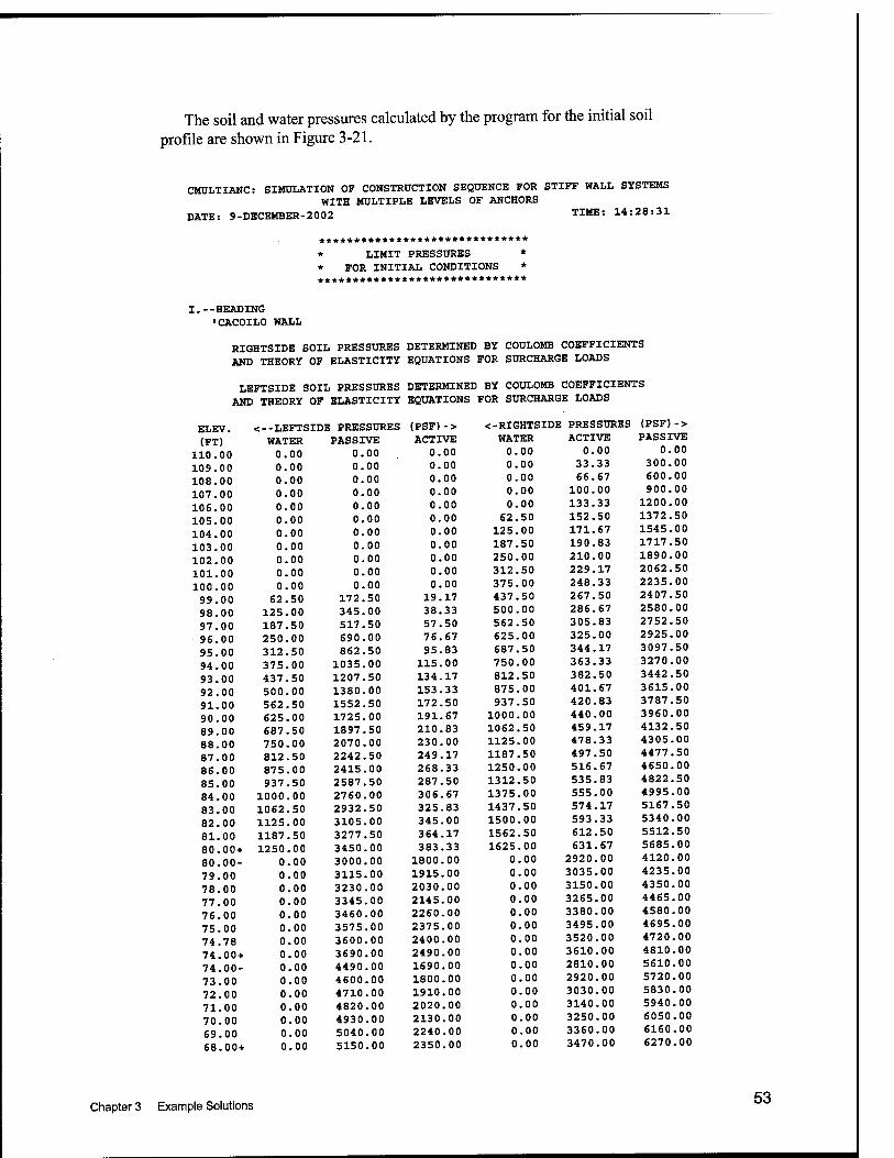
The soil and water pressures calculated by the program for the initial soil profile are shown in Figure 3-21.
CMULTIANC: SIMULATION OF CONSTRDCTION SEQUENCE FOR STIFF WALL SYSTEMS WITH MULTIPLE LEVELS OF ANCHORS
DATE: 9-DECEMBER-2002 TIME: 14:28:31
****************************** * LIMIT PRESSURES * * FOR INITIAL CONDITIONS * ******************************
-HEADING 'CACOILO WALL
RIGHTSIDE SOIL PRESSURES DETERMINED BY COULOMB COEFFICIENTS AND THEORY OP ELASTICITY EQUATIONS FOR SURCHARGE LOADS
LEFTSIDE SOIL PRESSURES DETERMINED BY COULOMB COEFFICIENTS AND THEORY OF ELASTICITY EQUATIONS FOR SURCHARGE LOADS
ELEV. <--LEFTSIDE PRESSURES (PSF)-> <-RIGHTSIDE PRESSURES (PSF)->
(FT) WATER PASSIVE ACTIVE WATER ACTIVE PASSIVE
110.00 0.00 0.00 0.00 0.00 0.00 0.00
109.00 0.00 0.00 0.00 0.00 33.33 300.00
108.00 0.00 0.00 0.00 0.00 66.67 600.00
107.00 0.00 0.00 0.00 0.00 100.00 900.00
106.00 0.00 0.00 0.00 0.00 133.33 1200.00
105.00 0.00 0.00 0.00 62.50 152.50 1372.50
104.00 0.00 0.00 0.00 125.00 171.67 1545.00
103.00 0.00 0.00 0.00 187.50 190.83 1717.50
102.00 0.00 0.00 0.00 250.00 210.00 1890.00
101.00 0.00 0.00 0.00 312.50 229.17 2062.50
100.00 0.00 0.00 0.00 375.00 248.33 2235.00
99.00 62.50 172.50 19.17 437.50 267.50 2407.50
98.00 125.00 345.00 38.33 500.00 286.67 2580.00
97.00 187.50 517.50 57.50 562.50 305.83 2752.50
96.00 250.00 690.00 76.67 625.00 325.00 2925.00
95.00 312.50 862.50 95.83 687.50 344.17 3097.50
94.00 375.00 1035.00 115.00 750.00 363.33 3270.00
93.00 437.50 1207.50 134.17 812.50 382.50 3442.50
92.00 500.00 1380.00 153.33 875.00 401.67 3615.00
91.00 562.50 1552.50 172.50 937.50 420.83 3787.50
90.00 625.00 1725.00 191.67 1000.00 440.00 3960.00
89.00 687.50 1897.50 210.83 1062.50 459.17 4132.50
88.00 750.00 2070.00 230.00 1125.00 478.33 4305.00
87.00 812.50 2242.50 249.17 1187.50 497.50 4477.50
86.00 875.00 2415.00 268.33 1250.00 516.67 4650.00
85.00 937.50 2587.50 287.50 1312.50 535.83 4822.50
84.00 1000.00 2760.00 306.67 1375.00 555.00 4995.00
83.00 1062.50 2932.50 325.83 1437.50 574.17 5167.50
82.00 1125.00 3105.00 345.00 1500.00 593.33 5340.00
81.00 1187.50 3277.50 364.17 1562.50 612.50 5512.50
80.00+ 1250.00 3450.00 383.33 1625.00 631.67 5685.00
80.00- 0.00 3000.00 1800.00 0.00 2920.00 4120.00
79.00 0.00 3115.00 1915.00 0.00 3035.00 4235.00
78.00 0.00 3230.00 2030.00 0.00 3150.00 4350.00
77.00 0.00 3345.00 2145.00 0.00 3265.00 4465.00
76.00 0.00 3460.00 2260.00 0.00 3380.00 4580.00
75.00 0.00 3575.00 2375.00 0.00 3495.00 4695.00
74.78 0.00 3600.00 2400.00 0.00 3520.00 4720.00
74.00+ 0.00 3690.00 2490.00 0.00 3610.00 4810.00
74.00- 0.00 4490.00 1690.00 0.00 2810.00 5610.00
73.00 0.00 4600.00 1800.00 0.00 2920.00 5720.00
72.00 0.00 4710.00 1910.00 0.00 3030.00 5830.00
71.00 0.00 4820.00 2020.00 0.00 3140.00 5940.00
70.00 0.00 4930.00 2130.00 0.00 3250.00 6050.00
69.00 0.00 5040.00 2240.00 0.00 3360.00 6160.00
68.00+ 0.00 5150.00 2350.00 0.00 3470.00 6270.00
Chapter 3 Example Solutions 53
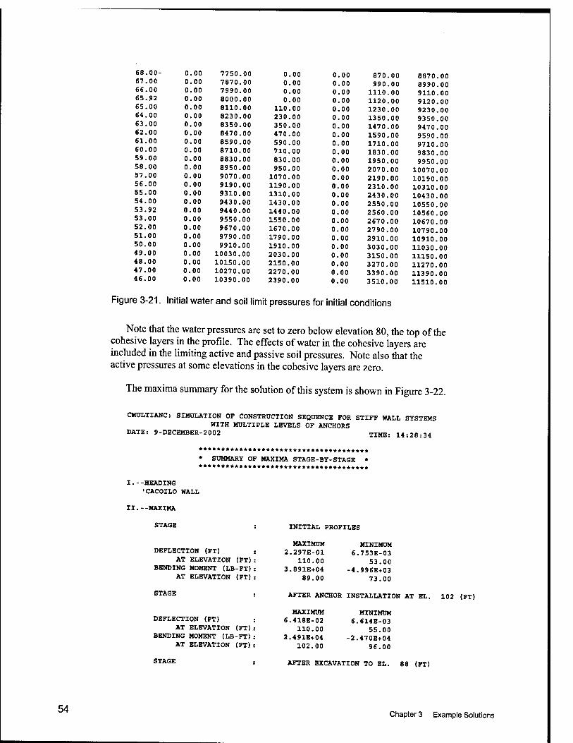
68.00- 0.00 7750.00 0.00 0.00 870.00 8870.00 67.00 0.00 7870.00 0.00 0.00 990.00 8990.00 66.00 0.00 7990.00 0.00 0.00 1110.00 9110.00 65.92 0.00 8000.00 0.00 0.00 1120.00 9120.00 65.00 0.00 8110.00 110.00 0.00 1230.00 9230.00 64.00 0.00 8230.00 230.00 0.00 1350.00 9350.00 63.00 0.00 8350.00 350.00 0.00 1470.00 9470.00 62.00 0.00 8470.00 470.00 0.00 1590.00 9590.00 61.00 0.00 8590.00 590.00 0.00 1710.00 9710.00 60.00 0.00 8710.00 710.00 0.00 1830.00 9830.00 59.00 0.00 8830.00 830.00 0.00 1950.00 9950.00 58.00 0.00 8950.00 950.00 0.00 2070.00 10070.00 57.00 0.00 9070.00 1070.00 0.00 2190.00 10190.00 56.00 0.00 9190.00 1190.00 0.00 2310.00 10310.00 55.00 0.00 9310.00 1310.00 0.00 2430.00 10430.00 54.00 0.00 9430.00 1430.00 0.00 2550.00 10550.00 53.92 0.00 9440.00 1440.00 0.00 2560.00 10560.00 53.00 0.00 9550.00 1550.00 0.00 2670.00 10670.00 52.00 0.00 9670.00 1670.00 0.00 2790.00 10790.00 51.00 0.00 9790.00 1790.00 0.00 2910.00 10910.00 50.00 0.00 9910.00 1910.00 0.00 3030.00 11030.00 49.00 0.00 10030.00 2030.00 0.00 3150.00 11150.00 48.00 0.00 10150.00 2150.00 0.00 3270.00 11270.00 47.00 0.00 10270.00 2270.00 0.00 3390.00 11390.00 46.00 0.00 10390.00 2390.00 0.00 3510.00 11510.00
Figure 3-21. Initial water and soil limit pressures for initial conditions
Note that the water pressures are set to zero below elevation 80, the top of the cohesive layers in the profile. The effects of water in the cohesive layers are included in the limiting active and passive soil pressures. Note also that the active pressures at some elevations in the cohesive layers are zero.
The maxima summary for the solution of this system is shown in Figure 3-22.
CMULTIANC: SIMULATION OF CONSTRUCTION SEQUENCE FOR STIFF WALL SYSTEMS WITH MULTIPLE LEVELS OF ANCHORS
DATE: 9-DECEMBER-2002 TIME: 14:28:34
************************************** * SUMMARY OF MAXIMA STAGE-BY-STAGE *
I. - -HEADING 'CACOILO WALL
II.--MAXIMA
STAGE INITIAL PROFILES
DEFLECTION (FT) AT ELEVATION (FT)
BENDING MOMENT (LB-FT) AT ELEVATION (FT)
MAXIMUM 2.297E-01
110.00 3.891E'f04
89.00
MINIMUM 6.753E-03
53.00 -4.996E+03
73.00
STAGE AFTER ANCHOR INSTALLATION AT EL. 102 (FT)
DEFLECTION (FT) AT ELEVATION (FT)
BENDING MOMENT (LB-FT) AT ELEVATION (FT)
STAGE
MAXIMUM 6.418E-02
110.00 2.491E+04
102.00
MINIMUM 6.614E-03
55.00 -2.470E+04
96.00
AFTER EXCAVATION TO EL. 88 (FT)
54 Chapter 3 Example Solutions
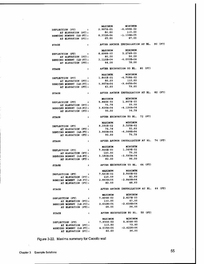
DEFLECTION (FT) AT ELEVATION (FT)
BENDING MOMENT (LB-FT) AT ELEVATION (FT)
STAGE
DEFLECTION (FT) AT ELEVATION (FT)
BENDING MOMENT (LB-FT) AT ELEVATION (FT)
MAXIMUM 2.987E-01
86.00 8.332E+04
65.00
MINIMUM -6.496E-02
110.00 -1.138E+05
87.00
AFTER ANCHOR INSTALLATION AT EL. 90 (FT)
MAXIMUM 8.698E-02
80.00 3.115E+04
64.00
MINIMUM 1.274E-02
56.00 -4.093E+04
78.00
STAGE AFTER EXCAVATION TO EL. 80 (FT)
DEFLECTION (FT) AT ELEVATION (FT)
BENDING MOMENT (LB-FT) AT ELEVATION (FT)
STAGE
MAXIMUM 1.860E-01
80.00 5.987E+04
63.00
MINIMUM -4.708E-02
110.00 -9.445E+04
79.00
AFTER ANCHOR INSTALLATION AT EL. 82 (FT)
DEFLECTION (FT) AT ELEVATION (FT)
BENDING MOMENT (LB-FT) AT ELEVATION (FT)
MAXIMUM 5.84eE-02
74.78 3.426E+04
90.00
MINIMUM 1.807E-02
55.00 -4.126E+04
74.78
STAGE AFTER EXCAVATION TO EL. 72 (FT)
DEFLECTION (FT) AT ELEVATION (FT)
BENDING MOMENT (LB-FT) AT ELEVATION (FT)
STAGE
MAXIMUM .350E-02
74.78 .980E+04
90.00
MINIMUM 2.325E-02
51.00 -6.548E+04
74.78
AFTER ANCHOR INSTALLATION AT EL. 74 (FT)
DEFLECTION (FT) AT ELEVATION (FT)
BENDING MOMENT (LB-FT) AT ELEVATION (FT)
MAXIMUM 7.866E-02
110.00 3.186E+04
82.00
MINIMUM 1.349E-02
79.00 -2.593E+04
96.00
STAGE AFTER EXCAVATION TO EL. 64 (FT)
DEFLECTION (FT) AT ELEVATION (FT)
BENDING MOMENT (LB-FT) AT ELEVATION (FT)
STAGE
MAXIMUM 7.541E-02
110.00 3.863E+04
82.00
MINIMUM 2.060E-02
83.00 -2.840E+04
68.00
AFTER ANCHOR INSTALLATION AT EL. 66 (FT)
DEFLECTION (FT) AT ELEVATION (FT)
BENDING MOMENT (LB-FT) AT ELEVATION (FT)
STAGE
MAXIMUM 7.894E-02
110.00 3.652E+04
66.00
MINIMUM 2.837E-03
67.00 -2.616E+04
96.00
AFTER EXCAVATION TO EL. 58 (FT)
DEFLECTION (FT) AT ELEVATION (FT)
BENDING MOMENT (LB-FT) AT ELEVATION (FT)
MAXIMUM 7.930E-02
110.00 4.015E+04
66.00
MINIMUM 5.828E-03
73.00 -2.622E+04
96.00
Figure 3-22. Maxima summary for Cacoiio wall
Chapter 3 Example Solutions 55
References
Cacoilo, D., Tamaro, G., and Edinger, P. (1998). "Design and performance of a tied-back sheet pile wall in soft clay." Design and construction of earth retaining systems, Geotechnical Special Publication No. 83, American Society of Civil Engineers, Reston, VA, 14-25.
Clough, G. W., and Tsui, Y. (1974). "Performance of tied-back walls in clay," Journal of Geotechnical Engineering Division, Proceedings ASCE 100 (GT 12), 1259-73.
Dawkins,W. P. (1994a). "User's guide: Computer program for Winkler soil- structure interaction analysis of sheet-pile walls (CWALSSI)," Technical Report ITL-94-5, U.S. Army Engineer Waterways Experiment Station, Vicksburg, MS.
• (1994b). "User's guide: Computer program for analysis of beam- column structures with nonlinear supports (CBEAMC)," Technical Report ITL-94-6, U.S. Army Engineer Waterways Experiment Station, Vicksburg, MS.
Department of the Navy. (1982) (May). "Foundations and earth structures," Design Manual 7.2; NAVFAC DM-7.2. Department of the Navy, Naval Facilities Engineering Command, Alexandria, VA.
Ebeling, R. M., Azene, M., and Strom, R. W. (2002). "Simplified procedures for the design of tall, anchored flexible tieback walls," ERDC/ITL TR-02-9, U.S. Army Engineer Research and Development Center, Vicksburg, MS.
Federal Highway Administration (FHWA). U.S. Department of Transportation, McLean, VA.
FHWA-RD-81-150, "Permanent, ground anchors, Soletanche design criteria' [Pfister, Evans, Guillaud, and Davidson 1982].
FHWA-RD-97-130, "Design manual for permanent ground anchor walls" [Weatherby 1998a].
FHWA-RD-98-065, "Summary report of research on permanent ground anchor walls; Vol I, Current practice and limit equilibrium analysis" [Long, Weatherby, and Cording 1998].
56 References
FHWA-RD-98-066, "Summary report of research on permanent ground anchor walls; Vol II, Full-scale wall tests and a soil structure interaction model" [Weatherby, Chung, Kim, and Briaud 1998].
FHWA-RD-98-067, "Summary report of research on permanent ground anchor walls; Vol III, Model-scale wall tests and ground anchor tests" [Mueller, Long, Weatherby, Cording, Powers, and Briaud 1998].
FHWA-RD-98-068, "Summary report of research on permanent ground anchor walls; Vol IV, Conclusions and recommendations" [Weatherby 1998b].
FHWA-RD-75-128, "Lateral support systems and underpinning" [Goldberg, Jaworski, and Gordon 1975].
FHWA-SA-99-015, "Ground anchors and anchored systems," Geotechnical Engineering Circular No. 4 [Sabatini, Pass, Bachus 1999].
Haliburton, T. A. (1981). "Soil structure interaction: Numerical analysis of beams and beam-columns," Technical Publication No. 14, School of Civil Engineering, Oklahoma State University, Stillwater, OK.
Headquarters, U.S. Army Corps of Engineers. (1989). "Retaining and flood walls," Engineer Manual 1110-2-2502, Washington, DC.
Kerr, W. C, and Tamaro, G. J. (1990). "Diaphragm walls-Update on design and performance." Design and performance of earth retaining structures. ASCE Geotechnical Publication No. 25. American Society of Civil Engineers, Reston, VA.
Liao, S. C, and Neff, T. L. (1990). "Estimating lateral earth pressure for design of excavation supports." Proceedings, ASCE specialty conference; Design and performance of earth retaining structures, Geotechnical Special Publication No. 25. American Society of Civil Engineers, Reston, VA.
Munger, D. F., Jones, P. T., and Johnson, J. (1991). "Temporary tieback wall, Bonneville Navigation Lock," Structural Engineering Conference, U.S. Army Corps of Engineers, Washington, DC.
Ratay, R. T. (1996). Handbookof temporary structures in construction. McGraw-Hill, New York.
Strom, R. W., and Ebeling, R. M. (2001). "State of the practice in the design of tall, stiff, and flexible tieback retaining walls," Technical Report ERDC/ITL TR-01-1, U.S. Army Engineer Research and Development Center, Vicksburg, MS.
Strom, R.W., and Ebeling, R. M. (2002). "Simplified procedures for the design of tall, stiff tieback walls," ERDC/ITL TR-02-10, U.S. Army Engineer Research and Development Center, Vicksburg, MS.
References 57

Terzaghi, K. (1955). "Evaluation of coefficient of subgrade reaction," Geotechnique 5, 297-326.
Xanthakos, P. P. (1991). Ground anchors and anchored structures. John Wiley, New York, 686 pp.
Yoo, C. (2001). "Behavior of braced and anchored walls in soils overlying rock," Journal of Geotechnical and Geoenvironmental Engineering 127(3).
References

Appendix A Guide for Data Input
A.1 Introduction
A.1.1 Source of input
Input data may be supplied from a predefined data file or from the user's keyboard during execution. When data are entered from the keyboard, prompts are provided to indicate the amount and character of data to be entered.
A.1.2 Data editing
Input data may be edited at any time until the construction sequence is initiated. After the construction sequence is complete, on-line editing is again available. However, the left-side profile will have been altered due to excavation resulting in inconsistencies with other data items.
A.1.3 Input data file generation
After data have been entered from the user's keyboard, the program vwites all current input data to a temporary file in input file ft)rmat. The temporary input file may be saved as a permanent file.
A.1.4 Sections of input
When data are entered from the user's keyboard, data sections may be entered in any order. When data are suppUed from a predefined input file, sections must be entered in the ftillowing order:
a. Heading (Required).
h. Wall Segment Data (Required).
c. Anchor Data (Optional).
d. Soil Profile Data (Required).
e. Initial Water Data (Optional).
A1 Appendix A Guide for Data Input
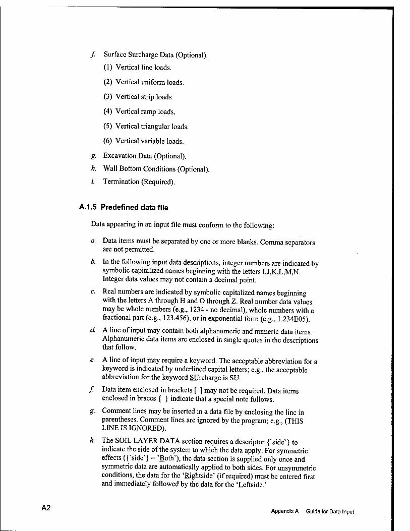
/ Surface Surcharge Data (Optional).
(1) Vertical line loads.
(2) Vertical uniform loads.
(3) Vertical strip loads.
(4) Vertical ramp loads.
(5) Vertical triangular loads.
(6) Vertical variable loads.
g. Excavation Data (Optional).
h. Wall Bottom Conditions (Optional).
/. Termination (Required).
A.1.5 Predefined data file
Data appearing in an input file must conform to the following:
a. Data items must be separated by one or more blanks. Comma separators are not permitted.
b. In the following input data descriptions, integer numbers are indicated by symbolic capitalized names beginning with the letters I,J,K,L,M,N. Integer data values may not contain a decimal point.
c. Real numbers are indicated by symbolic capitalized names beginning with the letters A through H and O through Z. Real number data values may be whole numbers (e.g., 1234 - no decimal), whole numbers with a fractional part (e.g., 123.456), or in exponential form (e.g., 1.234E05).
d A line of input may contain both alphanumeric and numeric data items. Alphanumeric data items are enclosed in single quotes in the descriptions that follow.
e. A line of input may require a keyword. The acceptable abbreviation for a keyword is indicated by underlined capital letters; e.g., the acceptable abbreviation for the keyword Surcharge is SU.
/ Data item enclosed in brackets [ ] may not be required. Data items enclosed in braces { } indicate that a special note follows.
g. Comment lines may be inserted in a data file by enclosing the line in parentheses. Comment lines are ignored by the program; e.g., (THIS LINE IS IGNORED).
h. The SOIL LAYER DATA section requires a descriptor {'side'} to indicate the side of the system to which the data apply. For symmetric effects ({'side'} = 'Both'), the data section is supplied only once and symmetric data are automatically applied to both sides. For unsymmetric conditions, the data for the 'Rightside' (if required) must be entered first and immediately followed by the data for the 'Leftside.'
A2 Appendix A Guide for Data Input
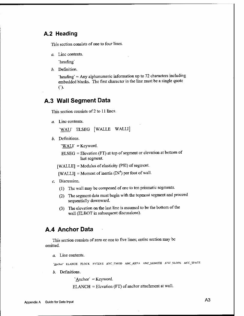
A.2 Heading
This section consists of one to four lines.
a. Line contents,
'heading'
b. Definition.
'heading' = Any alphanumeric information up to 72 characters including embedded blanks. The first character in the line must be a single quote
A.3 Wall Segment Data
This section consists of 2 to 11 lines.
a. Line contents.
'WALl' ELSEG [WALLE WALLi]
b. Definitions.
'WALl' = Keyword.
ELSEG = Elevation (FT) at top of segment or elevation at bottom of last segment.
[WALLE] = Modulus of elasticity (PSI) of segment.
[WALLI] = Moment of inertia (IN'') per foot of wall.
c. Discussion.
(1) The wall may be composed of one to ten prismatic segments.
(2) The segment data must begin with the topmost segment and proceed sequentially downward.
(3) The elevation on the last Une is assumed to be the bottom of the wall (ELBOT in subsequent discussions).
A.4 Anchor Data
This section consists of zero or one to five lines; entire section may be omitted.
a. Line contents.
•Anchor- ELANCH FLOCK FYTENS ANC_EMOD ANC_AREA ANC_LENGTH ANC_SLOPE ANC_SPACE
b. Definitions.
'Anchor' = Keyword.
ELANCH = Elevation (FT) of anchor attachment at wall.
A3 Appendix A Guide for Data Input ""
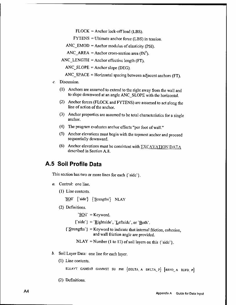
A4
FLOCK = Anchor lock-offload (LBS).
FYTENS = Ultimate anchor force (LBS) in tension.
ANCEMOD = Anchor modulus of elasticity (PSI).
ANC_AREA = Anchor cross-section area (IN^).
ANC_LENGTH = Anchor effective length (FT).
ANC_SLOPE = Anchor slope (DEG).
ANC_SPACE = Horizontal spacing between adjacent anchors (FT).
c. Discussion.
(1) Anchors are assumed to extend to the right away from the wall and to slope downward at an angle ANCSLOPE with the horizontal.
(2) Anchor forces (FLOCK and FYTENS) are assumed to act along the line of action of the anchor.
(3) Anchor properties are assumed to be total characteristics for a single anchor.
(4) The program evaluates anchor effects "per foot of wall."
(5) Anchor elevations must begin with the topmost anchor and proceed sequentially downward.
(6) Anchor elevations must be consistent with EXCAVATION DATA described in Section A.8.
A.5 Soil Profile Data
This section has two or more lines for each {'side'}.
a. Control: one line.
(1) Line contents.
'Sar {"side"} {'Strengths'} NLAY
(2) Definitions.
'SOil' = Keyword.
{'side'} = 'Rightside', 'Leftside', or 'Both'.
{'Strengths'} = Keyword to indicate that internal friction, cohesion, and wall friction angle are provided.
NLAY = Number (1 to 11) of soil layers on this {'side'}.
b. Soil Layer Data: one line for each layer.
(1) Line contents.
ELLAYT GAMSAT GAMMST SU PHI {DELTA_A DELTA_P} [REFD_A REFD_P]
(2) Definitions.
Appendix A Guide for Data Input
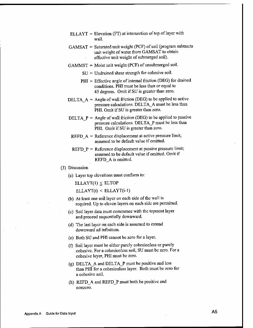
ELLAYT = Elevation (FT) at intersection of top of layer with wall.
GAMS AT = Saturated unit weight (PCF) of soil (program subtracts unit weight of water from GAMS AT to obtain effective unit weight of submerged soil).
GAMMST = Moist unit weight (PCF) of unsubmerged soil.
SU = Undrained shear strength for cohesive soil.
PHI = Effective angle of internal friction (DEG) for drained conditions. PHI must be less than or equal to 45 degrees. Omit if SU is greater than zero.
DELTA_A = Angle of wall friction (DEG) to be appUed to active pressure calculations. DELTA_A must be less than PHI. Omit if SU is greater than zero.
DELTA_P = Angle of wall friction (DEG) to be applied to passive pressure calculations. DELTA_P must be less than PHI. Omit if SU is greater than zero.
REFD_A = Reference displacement at active pressure limit; assumed to be default value if omitted.
REFD_P = Reference displacement at passive pressure limit; assumed to be default value if omitted. Omit if REFD_A is omitted.
(3) Discussion
(a) Layer top elevations must conform to:
ELLAYT(l) < ELTOP
ELLAYT(i) < ELLAYT(i-l)
(b) At least one soil layer on each side of the wall is required. Up to eleven layers on each side are permitted.
(c) Soil layer data must commence with the topmost layer and proceed sequentially downward.
(d) The last layer on each side is assumed to extend downward ad infinitum.
(e) Both SU and PHI cannot be zero for a layer.
(f) Soil layer must be either purely cohesionless or purely cohesive. For a cohesionless soil, SU must be zero. For a cohesive layer, PHI must be zero.
(g) DELTA_A and DELTA_P must be positive and less than PHI for a cohesionless layer. Both must be zero for a cohesive soil.
(h) REFD_A and REFD_P must both be positive and nonzero.
Appendix A Guide for Data Input A5
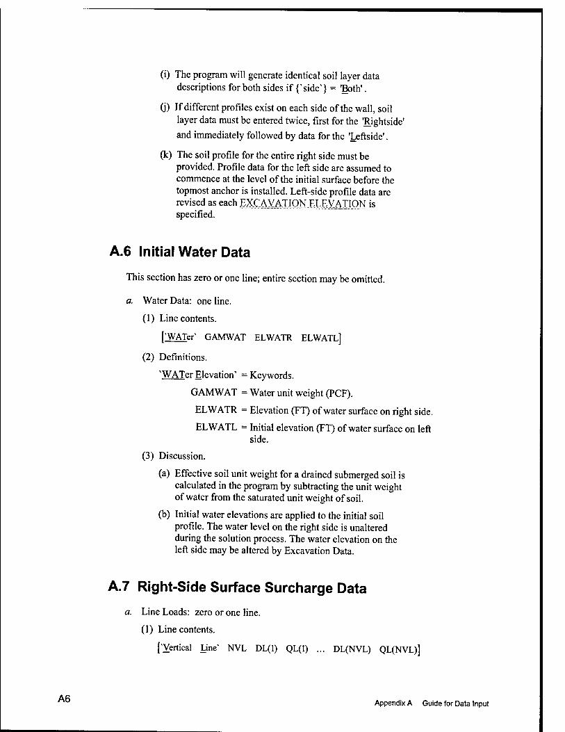
(i) The program will generate identical soil layer data descriptions for both sides if {'side'} = 'Both'.
(j) If different profiles exist on each side of the wall, soil layer data must be entered twice, first for the 'Rightside'
and immediately followed by data for the 'Leftside'.
(k) The soil profile for the entire right side must be provided. Profile data for the left side are assumed to commence at the level of the initial surface before the topmost anchor is installed. Left-side profile data are revised as each MSikVLAIIfiM JLIMIKM is specified.
A.6 Initial Water Data
This section has zero or one line; entire section may be omitted.
a. Water Data: one line.
(1) Line contents.
['WATer' GANfWAT ELWATR ELWATL]
(2) Definitions.
'WATer Elevation' = Keywords.
GAMWAT = Water unit weight (PCF).
ELWATR = Elevation (FT) of water surface on right side.
ELWATL = Initial elevation (FT) of water surface on left side.
(3) Discussion.
(a) Effective soil unit weight for a drained submerged soil is calculated in the program by subtracting the unit weight of water from the saturated unit weight of soil.
(b) Initial water elevations are applied to the initial soil profile. The water level on the right side is unaltered during the solution process. The water elevation on the left side may be altered by Excavation Data.
A.7 Right-Side Surface Surcharge Data
a. Line Loads: zero or one line.
(1) Line contents.
['Vertical Line' NVL DL(1) QL(1) ... DL(NVL) QL(NVL)]
A6 Appendix A Guide for Data Input
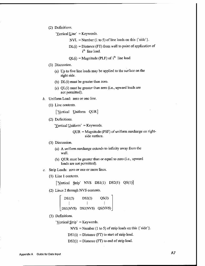
(2) Definitions.
'Vertical Line' = Keywords.
NVL = Number (1 to 5) of line loads on this {'side'}.
DL(i) = Distance (FT) from wall to point of application of i"" line load.
QL(i) = Magnitude (PLF) of i* line load
(3) Discussion.
(a) Up to five line loads may be applied to the surface on the right side.
(b) DL(i) must be greater than zero.
(c) QL(i) must be greater than zero (i.e., upward loads are not permitted).
b. Uniform Load: zero or one line.
(1) Line contents.
['Vertical Uniform QUR]
(2) Definitions.
'Vertical Uniform' = Keywords.
QUR = Magnitude (PSF) of uniform surcharge on right- side surface.
(3) Discussion.
(a) A uniform surcharge extends to infinity away from the wall.
(b) QUR must be greater than or equal to zero (i.e., upward loads are not permitted).
c. Strip Loads: zero or one or more lines.
(1) Line 1 contents.
['Vertical Strip' NVS DSl(l) DS2(1) QS(1)]
(2) Lines 2 through NVS contents.
DS1(2) DS2(2) QS(2)
DS1(NVS) DS2(NVS) QS(NVS)_
(3) Definitions.
'Vertical Strip' = Keywords.
NVS = Number (1 to 5) of strip loads on this {'side'}.
DSl(i) = Distance (FT) to start of strip load.
DS2(i) = Distance (FT) to end of strip load.
Appendix A Guide for Data Input "'
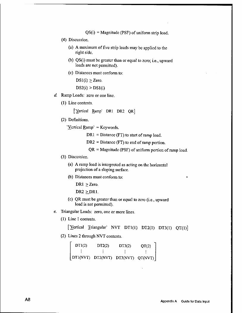
QS(i) = Magnitude (PSF) of uniform strip load.
(4) Discussion.
(a) A maximum of five strip loads may be applied to the right side.
(b) QS(i) must be greater than or equal to zero; i.e., upward loads are not permitted).
(c) Distances must conform to:
DSI(i) >Zero.
DS2(i) >DSl(i)
d. Ramp Loads: zero or one line.
(1) Line contents.
['Vertical Ramp" DRl DR2 QR]
(2) Definitions.
'Vertical Ramp' = Keywords.
DRl = Distance (FT) to start of ramp load.
DR2 = Distance (FT) to end of ramp portion.
QR = Magnitude (PSF) of uniform portion of ramp load.
(3) Discussion.
(a) A ramp load is interpreted as acting on the horizontal projection of a sloping surface.
(b) Distances must conform to:
DRl >Zero.
DR2 ^DRl.
(c) QR must be greater than or equal to zero (i.e., upward load is not permitted).
e. Triangular Loads: zero, one or more lines.
(1) Line 1 contents.
['Vertical Triangular' NVT DTI (I) DT2(1) DT3(1) QT(1)]
(2) Lines 2 through NVT contents.
DTI (2) DT2(2) DT3(2) QT(2)
DTI (NVT) DT2(NVT) DT3(NVT) QT(NVT)
A8 Appendix A Guide for Data Input
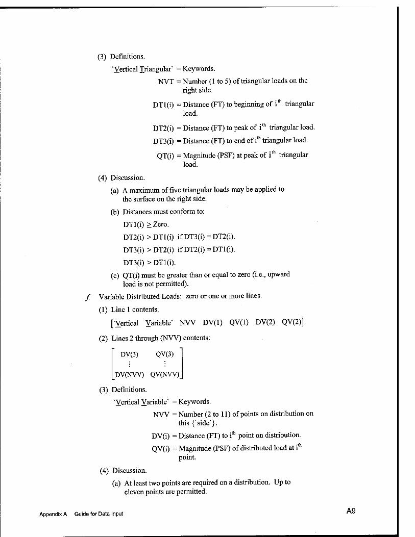
(3) Definitions.
'Vertical Triangular' = Keywords.
NVT = Number (1 to 5) of triangular loads on the right side.
DTl(i) = Distance (FT) to beginning of i* triangular load.
DT2(i) = Distance (FT) to peak of i* triangular load.
DT3(i) = Distance (FT) to end of i* triangular load.
QT(i) = Magnitude (PSF) at peak of i* triangular load.
(4) Discussion.
(a) A maximum of five triangular loads may be applied to the surface on the right side.
(b) Distances must conform to:
DTl(i) >Zero.
DT2(i) >DTl(i) ifDT3(i) = DT2(i).
DT3(i) >DT2(i) if DT2(i) = DTl(i).
DT3(i) > DTl(i).
(c) QT(i) must be greater than or equal to zero (i.e., upward load is not permitted).
/ Variable Distributed Loads: zero or one or more lines.
(1) Line 1 contents.
['Vertical Variable' NW DV(1) QV(1) DV(2) QV(2)]
(2) Lines 2 through (NW) contents:
DV(3) QV(3)
DV(NVV) QVCNVV)_
(3) Definitions.
'Vertical Variable' = Keywords.
NW = Number (2 to 11) of points on distribution on this {'side'}.
DV(i) = Distance (FT) to i* point on distribution.
QV(i) = Magnitude (PSF) of distributed load at i* point.
(4) Discussion.
(a) At least two points are required on a distribution. Up to eleven points are permitted.
Appendix A Guide for Data Input A9
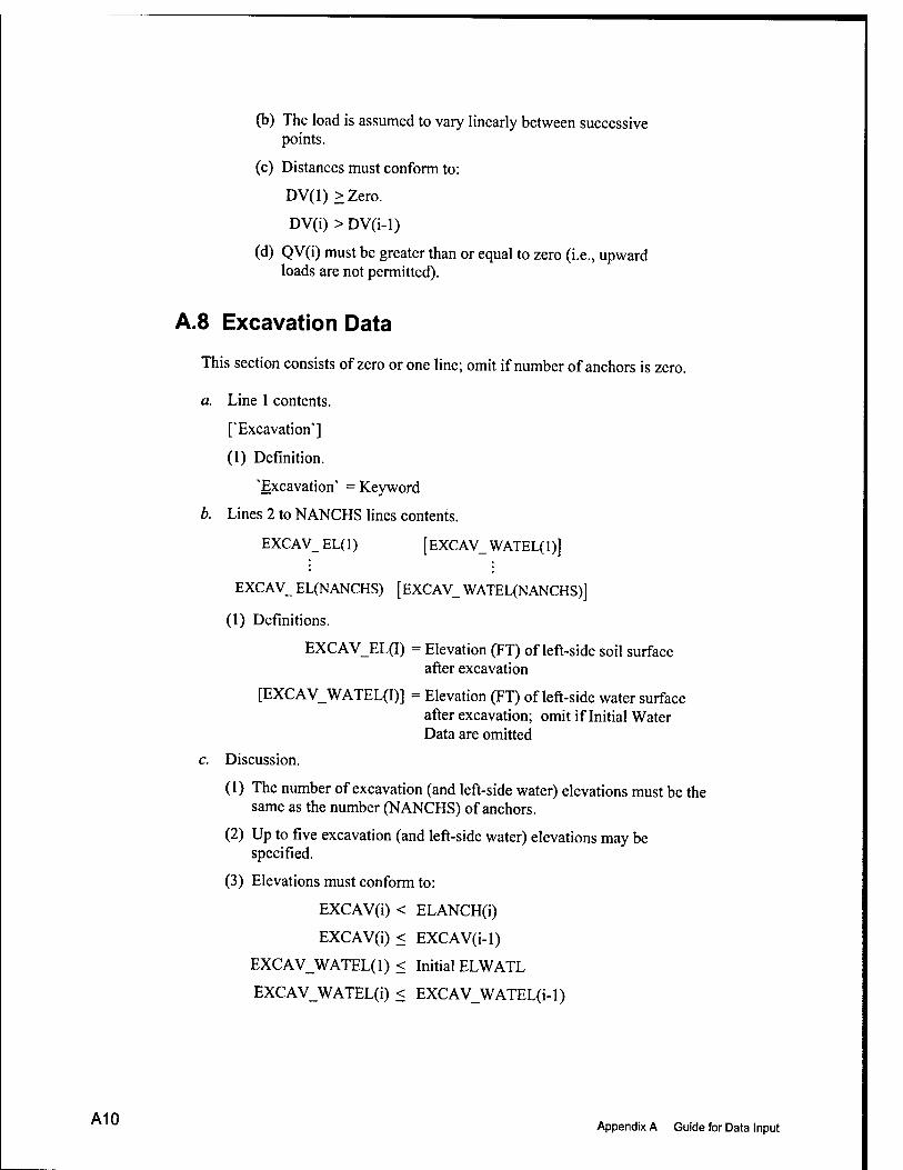
(b) The load is assumed to vary linearly between suecessive points.
(c) Distances must conform to:
DV(l)>Zero.
DV(i)>DV(i-l)
(d) QV(i) must be greater than or equal to zero (i.e., upward loads are not permitted).
A.8 Excavation Data
This section consists of zero or one line; omit if number of anchors is zero.
a. Line 1 contents.
['Excavation']
(1) Definition.
'Excavation' = Keyword
b. Lines 2 to NANCHS lines contents.
EXCAV_EL(1) [EXCAV_WATEL(1)]
EXC AV_ EL(NANCHS) [ EXCAV_ WATEL(N ANCHS)]
(1) Definitions.
EXCAV_EL(I) = Elevation (FT) of left-side soil surface after excavation
[EXCAV_WATEL(I)] = Elevation (FT) of left-side water surface after excavation; omit if Initial Water Data are omitted
c. Discussion.
(1) The number of excavation (and left-side water) elevations must be the same as the number (NANCHS) of anchors.
(2) Up to five excavation (and left-side water) elevations may be specified.
(3) Elevations must conform to:
EXCAV(i) < ELANCH(i)
EXCAV(i) < EXCAV(i-l)
EXCAV_WATEL(1) < Initial ELWATL
EXCAV_WATEL(i) < EXCAV_WATEL(i-l)
A10 Appendix A Guide for Data Input
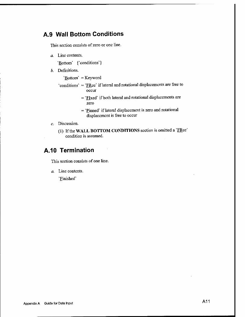
A.9 Wall Bottom Conditions
This section consists of zero or one line.
a. Line contents.
'Bottom' {'conditions'}
b. Definitions.
'Bottom' = Keyword
'conditions' = 'FRee' if lateral and rotational displacements are free to occur
= 'Fixed' if both lateral and rotational displacements are zero
= 'Pinned' if lateral displacement is zero and rotational displacement is free to occur
c. Discussion.
(1) If the WALL BOTTOM CONDITIONS section is omitted a 'FRee' condition is assumed.
A.10 Termination
This section consists of one line.
a. Line contents.
'Finished'
A11 Appendix A Guide for Data Input "'
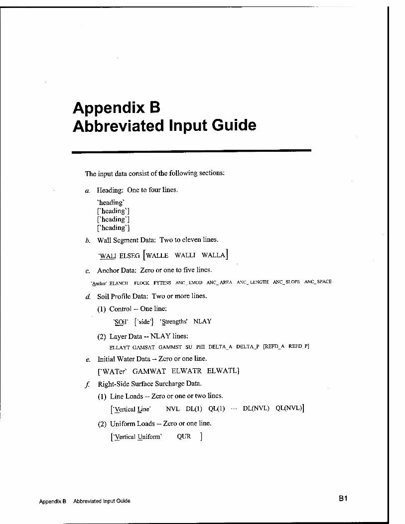
Appendix B Abbreviated Input Guide
The input data consist of the following sections:
a. Heading: One to four lines.
'heading' ['heading'] ['heading'] ['heading']
b. Wall Segment Data: Two to eleven lines.
'WAU ELSEG [WALLE WALLI WALLA]
c. Anchor Data: Zero or one to five lines.
■Anchor- ELANCH FLOCK FYTENS ANC_ EMOD ANC_AREA ANC_ LENGTH ANC_ SLOPE ANC_ SPACE
d Soil Profile Data: Two or more lines.
(1) Control - One line:
'Sar {'side'} 'Strengths' NLAY
(2) Layer Data -- NLAY lines: ELLAYT GAMSAT GAMMST SU PHI DELTA_A DELTA_P [REFD_A REFD_P]
e. Initial Water Data ~ Zero or one line.
['WATer' GAMWAT ELWATR ELWATL]
/ Right-Side Surface Surcharge Data.
(1) Line Loads ~ Zero or one or two lines.
['Vertical Line' NVL DL(1) QL(1) - DL(NVL) QL(NVL)]
(2) Uniform Loads ~ Zero or one line.
['Vertical Uniform' QUR ]
R1 Appendix B Abbreviated Input Guide " '
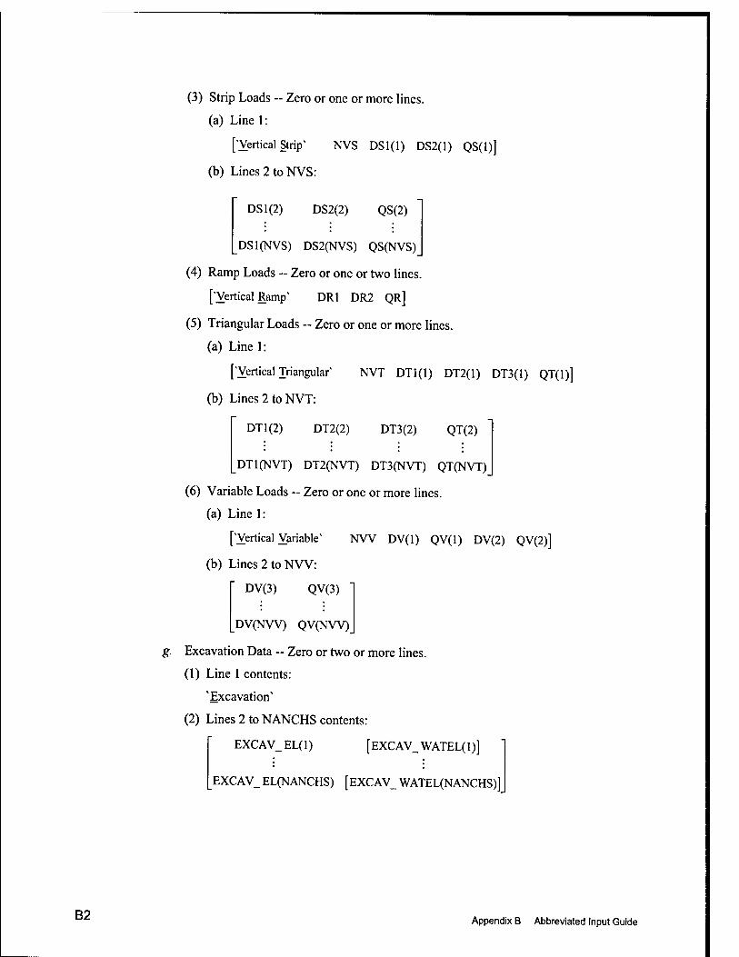
(3) Strip Loads ~ Zero or one or more lines.
(a) Line 1:
['Vertical Strip- NVS DSI(l) DS2(1) QS(1)]
(b) Lines 2 to NVS:
DS1(2) DS2(2) QS(2)
_DSI(NVS) DS2(NVS) QS(NVS)
(4) Ramp Loads ~ Zero or one or two lines.
['Vertical Ramp" DRl DR2 QR]
(5) Triangular Loads ~ Zero or one or more lines.
(a) Line 1:
['Vertical Triangular' NVT DTl(l) DT2(1) DT3(1) QT(1)]
(b) Lines 2 to NVT:
DTI (2) DT2(2) DT3(2) QT(2)
_DT1(NVT) DT2(NVT) DT3(NVT) QT(NVT)
(6) Variable Loads — Zero or one or more lines.
(a) Line 1:
['Vertical Variable' NW DV(1) QV(1) DV(2) QV(2)]
(b) Lines2toNVV:
DV(3) QV(3)
DV(NVV) QV(NW)
g. Excavation Data -- Zero or two or more lines.
(1) Line 1 contents:
'Excavation'
(2) Lines 2 to NANCHS contents:
EXCAV_EL(1) [EXCAV_WATEL(1)]
EXCAV_ EL(NANCHS) [EXCAV_ WATEL(NANCHS)]
B2 Appendix B Abbreviated Input Guide
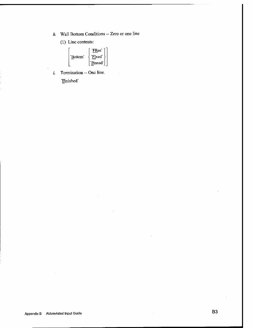
h. Wall Bottom Conditions ~ Zero or one line
(1) Line contents:
'Bottom"
'FRee" 'Fixed" 'Hrnied'
Termination ~ One line.
'Rnished'
Appendix B Abbreviated Input Guide B3
REPORTS PUBLISHED UNDER THE COMPUTER-AIDED STRUCTURAL ENGINEERING (CASE) PROJECT
Technical Report K-78-1
Instruction Report 0-79-2
Technical Report K-80-1
Technical Report K-80-2
Instruction Report K-80-1
Instruction Report K-80-3
Instruction Report K-80-4
Instnjction Report K-80-6
Instruction Report K-80-7
Technical Report K-80-4
Technical Report K-80-5
Instruction Report K-81-2
Instruction Report K-81-3
Instruction Report K-81-4
Instruction Report K-81-6
Instruction Report K-81-7
Instruction Report K-81-9
Technical Report K-81-2
Title Date
List of Computer Programs for Computer-Aided Structural Engineering Feb 1978
User's Guide: Computer Program with Interactive Graphics for Analysis Mar 1979 of Plane Frame Structures (CFRAME)
Survey of Bridge-Oriented Design Software Jan 1980
Evaluation of Computer Programs for the Design/Analysis of Highway Jan 1980 and Railway Bridges
User's Guide: Computer Program for Design/Review of Curvi-linear Feb 1980 Conduits/Culveris (CURCON)
A Three-Dimensional Finite Element Data Edit Program Mar 1980
A Three-Dimensional Stability Analysis/Design Program (3DSAD) Report 1: General Geometry Module Jun 1980 Report 3: General Analysis Module (CGAM) Jun 1982 Report 4: Special-Purpose Modules for Dams (CDAMS) Aug 1983
Basic User's Guide: Computer Program for Design and Analysis of Dec 1980 Inverted-T Retaining Walls and Floodwalls (TWDA)
User's Reference Manual: Computer Program for Design and Analysis of Dec 1980 Inverted-T Retaining Walls and Floodwalls (TWDA)
Documentation of Finite Element Analyses Report 1: Longview Outlet Works Conduit Dec 1980 Report 2: Anchored Wall Monolith, Bay Springs Lock Dec 1980
Basic Pile Group Behavior Dec 1980
User's Guide: Computer Program for Design and Analysis of Sheet Pile Walls by Classical Methods (CSHTWAL)
Report 1: Computational Processes Feb 1981 Report 2: Interactive Graphics Options Mar 1981
Validation Report: Computer Program for Design and Analysis of Feb 1981 Inverted-T Retaining Walls and Floodwalls (TWDA)
User's Guide: Computer Program for Design and Analysis of Cast-in- Mar 1981 Place Tunnel Linings (NEWTUN)
User's Guide: Computer Program for Optimum Nonlinear Dynamic Mar 1981 Design of Reinforced Concrete Slabs Under Blast Loading (CBARCS)
User's Guide: Computer Program for Design or Investigation of Mar 1981 Orthogonal Culverts (CORTCUL)
User's Guide: Computer Program for Three-Dimensional Analysis of Aug 1981 Building Systems (CTABS80)
Theoretical Basis for CTABS80: A Computer Program for Sep 1981 Three-Dimensional Analysis of Building Systems
(Continued)
1
REPORTS PUBLISHED UNDER THE COMPUTER-AIDED STRUCTURAL ENGINEERING (CASE) PROJECT
Instruction Report K-82-6
Instnjction Report K-82-7
Instruction Report K-83-1
Instruction Report K-83-2
Instruction Report K-83-5
Technical Report K-83-1
Technical Report K-83-3
Technical Report K-83-4
Instruction Report K-84-2
Instruction Report K-84-7
Instruction Report K-84-8
Instruction Report K-84-11
Technical Report K-84-3
Technical Report ATC-86-5
Technical Report ITL-87-2
Instruction Report ITL-87-2 (Revised)
Instruction Report ITL-87-1
Instnjction Report ITL-87-2
Technical Report ITL-87-6
Title Date
User's Guide: Computer Program for Analysis of Beam-Column Jun 1982 Structures with Nonlinear Supports (CBEAMC)
User's Guide: Computer Program for Bearing Capacity Analysis of Jun 1982 Shallow Foundations (CBEAR)
User's Guide: Computer Program with Interactive Graphics for Jan 1983 Analysis of Plane Frame Structures (CFRAME)
User's Guide: Computer Program for Generation of Engineering Jun 1983 Geometry (SKETCH)
User's Guide: Computer Program to Calculate Shear, Moment, and Jul 1983 Thrust (CSMT) from Stress Results of a Two-Dimensional Finite Element Analysis
Basic Pile Group Behavior Sep1983
Reference Manual: Computer Graphics Program for Generation of Sep 1983 Engineering Geometry (SKETCH)
Case Study of Six Major General-Purpose Finite Element Programs Oct 1983
User's Guide: Computer Program for Optimum Dynamic Design of Jan 1984 Nonlinear Metal Plates Under Blast Loading (CSDOOR)
User's Guide: Computer Program for Determining Induced Stresses Aug 1984 and Consolidation Settlements (CSETT)
Seepage Analysis of Confined Flow Problems by the Method of Sep 1984 Fragments (CFRAG)
User's Guide for Computer Program CGFAG, Concrete General Sep 1984 Flexure Analysis with Graphics
Computer-Aided Drafting and Design for Corps Structural Engineers Oct 1984
Decision Logic Table Formulation of ACI 318-77, Building Code Jun 1986 Requirements for Reinforced Concrete for Automated Constraint Processing, Volumes I and 11
A Case Committee Study of Finite Element Analysis of Concrete Flat Jan 1987 Slabs
User's Guide for Concrete Strength Investigation and Design Mar 1992 (CASTR) in Accordance with ACI 318-89
User's Guide: Computer Program for Two-Dimensional Analysis of U- Apr 1987 Frame Stnjctures (CUFRAM)
User's Guide: For Concrete Strength Investigation and Design May 1987 (CASTR) in Accordance with ACI 318-83
Finite-Element Method Package for Solving Steady-State Seepage May 1987 Problems
(Continued)
2
REPORTS PUBLISHED UNDER THE COMPUTER-AIDED STRUCTURAL ENGINEERING (CASE) PROJECT
Instruction Report ITL-87-3
Instruction Report ITL-87-4
Technical Report ITL-87-4
Instruction Report GL-87-1
Instruction Report ITL-87-5
Instruction Report ITL-87-6
Technical Report ITL-87-8
Instruction Report ITL-88-1
Technical Report ITL-88-1
Technical Report ITL-88-2
Instruction Report ITL-88-2
Instruction Report ITL-88-4
Instruction Report GL-87-1
Technical Report ITL-89-3
Title Date
User's Guide: A Three-Dimensional Stability Analysis/Design Program Jun 1987 (3DSAD) Module
Report 1: Revision 1: General Geometry Jun 1987 Report 2: General Loads Module Sep 1989 Report 6: Free-Body Module Sep 1989
User's Guide: 2-D Frame Analysis Link Program (LINK2D) Jun 1987
Finite Element Studies of a Horizontally Framed Miter Gate Aug 1987 Report 1: Initial and Refined Finite Element Models (Phases A,
B, and C), Volumes I and 11 Report 2: Simplified Frame Model (Phase D) Report 3: Alternate Configuration Miter Gate Finite Element
Studies-Open Section Report 4: Alternate Configuration Miter Gate Finite Element
Studies-Closed Sections Report 5: Alternate Configuration Miter Gate Finite Element
Studies-Additional Closed Sections Report 6: Elastic Buckling of Girders in Horizontally Framed
Miter Gates Report 7: Application and Summary
User's Guide: UTEXAS2 Slope-Stability Package; Volume 1, User's Aug 1987 Manual
Sliding Stability of Concrete Structures (CSLIDE) Oct 1987
Criteria Specifications for and Validation of a Computer Program for Dec 1987 the Design or Investigation of Horizontally Framed Miter Gates (CMITER)
Procedure for Static Analysis of Gravity Dams Using the Finite Jan 1988 Element Method - Phase la
User's Guide: Computer Program for Analysis of Planar Grid Feb 1988 Structures (CGRID)
Development of Design Formulas for Ribbed Mat Foundations on Apr 1988 Expansive Soils
User's Guide: Pile Group Graphics Display (CPGG) Postprocessor to Apr 1988 CPGA Program
User's Guide for Design and Investigation of Horizontally Framed Jun 1988 Miter Gates (CMITER)
User's Guide for Revised Computer Program to Calculate Shear, Sep 1988 Moment, and Thrust (CSMT)
User's Guide: UTEXAS2 Slope-Stability Package; Volume 11, Theory Feb 1989
User's Guide: Pile Group Analysis (CPGA) Computer Group Jul 1989
(Continued)
3
REPORTS PUBLISHED UNDER THE COMPUTER-AIDED STRUCTURAL ENGINEERING (CASE) PROJECT
Technical Report ITL-89-4
Technical Report ITL-89-5
Technical Report ITL-89-6
Contract Report ITL-89-1
Instruction Report ITL-90-1
Instruction Report ITL-90-2
Instruction Report ITL-90-3
Instruction Report ITL-90-6
Technical Report ITL-91-3
Instruction Report ITL-91-1
Technical Report ITL-92-2
Technical Report ITL-92-4
Instruction Report ITL-92-3
Title
CBASIN-Structural Design of Saint Anthony Falls Stilling Basins According to Corps of Engineers Criteria for Hydraulic Structures; Computer Program X0098
CCHAN-Stmctural Design of Rectangular Channels According to Corps of Engineers Criteria for Hydraulic Structures; Computer Program X0097
The Response-Spectrum Dynamic Analysis of Gravity Dams Using the Finite Element Method; Phase 11
State of the Art on Expert Systems Applications in Design, Construction, and Maintenance of Structures
User's Guide: Computer Program for Design and Analysis of Sheet Pile Walls by Classical Methods (CWALSHT)
User's Guide: Pile Group-Concrete Pile Analysis Program (CPGC) Preprocessor to CPGA Program
Investigation and Design of U-Frame Structures Using Program CUFRBC
Volume A: Program Criteria and Documentation Volume B: User's Guide for Basins Volume C: User's Guide for Channels
User's Guide: Computer Program for Two-Dimensional Analysis of U- Frame or W-Frame Structures (CWFRAM)
Application of Finite Element, Grid Generation, and Scientific Visualization Techniques to 2-D and 3-D Seepage and Groundwater Modeling
User's Guide: Computer Program for Design and Analysis of Sheet- Pile Walls by Classical Methods (CWALSHT) Including Rowe's Moment Reduction
Finite Element Modeling of Welded Thick Plates for Bonneviile Navigation Lock
Introduction to the Computation of Response Spectrum for Earthquake Loading
Concept Design Example, Computer-Aided Structural Modeling (CASM)
Report 1 Report 2 Report 3
Scheme A Scheme B Scheme C
Instruction Report ITL-92-4
Instnjction Report ITL-92-5
User's Guide: Computer-Aided Structural Modeling (CASM) - Version 3.00
Tutorial Guide: Computer-Aided Structural Modeling (CASM) • Version 3.00
Date
Aug 1989
Aug 1989
Aug 1989
Sep1989
Feb 1990
Jun 1990
May 1990 May 1990 May 1990
Sep 1990
Sep 1990
Oct 1991
May 1992
Jun 1992
Jun 1992 Jun 1992 Jun 1992
Apr 1992
Apr 1992
(Continued)
4
REPORTS PUBLISHED UNDER THE COMPUTER-AIDED STRUCTURAL ENGINEERING (CASE) PROJECT
Contract Report ITL-92-1
Technical Report ITL-92-7
Contract Report ITL-92-2
Contract Report ITL-92-3
Instruction Report GL-87-1
Technical Report ITL-92-11
Technical Report ITL-92-12
Instruction Report GL-87-1
Technical Report ITL-93-1
Technical Report ITL-93-2
Technical Report ITL-93-3
Instruction Report ITL-93-3
Instruction Report ITL-93-4
Technical Report ITL-94-2
Instoiction Report ITL-94-1
Instruction Report ITL-94-2
Technical Report ITL-94-4
Technical Report lTL-94-5
Instruction Report ITL-94-5
Title
Optimization of Steel Pile Foundations Using Optimality Criteria
Refined Stress Analysis of Melvin Price Locks and Dam
Knowledge-Based Expert System for Selection and Design of Retaining Structures
Evaluation of Thermal and Incremental Construction Effects for Monoliths AL-3 and AL-5 of the Melvin Price Loclcs and Dam
User's Guide: UTEXAS3 Slope-Stability Package; Volume IV, User's Manual
The Seismic Design of Waterfront Retaining Structures
Computer-Aided, Field-Verified Structural Evaluation Report 1: Development of Computer Modeling Techniques for
Miter Lock Gates Report 2: Field Test and Analysis Correlation at John Hollis
Bankhead Lock and Dam Report 3: Field Test and Analysis Correlation of a Vertically
Framed Miter Gate at Emsworth Lock and Dam
Users Guide: UTEXAS3 Slope-Stability Package; Volume III, Example Problems
Theoretical Manual for Analysis of Arch Dams
Steel Structures for Civil Works, General Considerations for Design and Rehabilitation
Soil-Structure Interaction Study of Red River Lock and Dam No. 1 Subjected to Sediment Loading
User's Manual-ADAP, Graphics-Based Dam Analysis Program
Load and Resistance Factor Design for Steel Miter Gates
User's Guide for the Incremental Constmction, Soil-Structure Interaction Program SOILSTRUCT with Far-Field Boundary Elements
Tutorial Guide: Computer-Aided Structural Modeling (CASM); Version 5.00
User's Guide: Computer-Aided Structural Modeling (CASM); Version 5.00
Dynamics of Intake Towers and Other MDOF Structures Under Earthquake Loads: A Computer-Aided Approach
Procedure for Static Analysis of Gravity Dams Including Foundation Effects Using the Finite Element Method - Phase 1 B
User's Guide: Computer Program for Winkler Soil-Structure Interaction Analysis of Sheet-Pile Walls (CWALSSI)
Date
Jun 1992
Sep 1992
Sep1992
Sep1992
Nov1992
Nov1992
Nov 1992
Dec 1992
Dec 1993
Dec 1992
Jul 1993
Aug 1993
Sep1993
Aug 1993
Oct 1993
Mar 1994
Apr 1994
Apr 1994
Jul 1994
Jul 1994
Nov 1994
(Continued)
5
REPORTS PUBLISHED UNDER THE COMPUTER-AIDED STRUCTURAL ENGINEERING (CASE) PROJECT
Title Date
Instaiction Report ITL-94-6 User's Guide: Computer Program for Analysis of Beam-Column Structures with Nonlinear Supports (CBEAMC)
Nov 1994
Instruction Report ITL-94-7 User's Guide to CTWALL - A Microcomputer Program for the Analysis of Retaining and Flood Walls
Dec 1994
Contract Report ITL-95-1 Comparison of Barge Impact Experimental and Finite Element Results for the Lower Miter Gate of Lock and Dam 26
Jun1995
Technical Report ITL-95-5 Soil-Structure Interaction Parameters for Structured/Cemented Silts Aug 1995
Instruction Report ITL-95-1 User's Guide: Computer Program for the Design and Investigation of Horizontally Framed Miter Gates Using the Load and Resistance Factor Criteria (CMITER-LRFD)
Aug1995
Technical Report ITL-95-8 Constitutive Modeling of Concrete for Massive Concrete Stmctures, A Simplified Overview
Sep 1995
Instmction Report ITL-96-1 Use's Guide: Computer Program for Two-Dimensiona! Dynamic Analysis of U-Frame or W-Frame Structures (CDWFRM)
Jun 1996
Instruction Report ITL-96-2 Computer-Aided Structural Modeling (CASM), Version 6.00 Report 1: Tutorial Guide Report 2: User's Guide Reports: Scheme A Report 4: Scheme B Reports: Scheme C
Jun 1996
Technical Report ITL-96-8 Hyperbolic Stress-Strain Parameters for Structured/Cemented Silts Aug 1996
Instmction Report ITL-96-3 User's Guide: Computer Program for the Design and Investigation of Horizontally Framed Miter Gates Using the Load and Resistance Factor Criteria (CMITERW-LRFD) Windows Version
Sep 1996
Instmction Report ITL-97-1 User's Guide: Computer Aided Inspection Fomris for Hydraulic Steel Stmctures (CAIF-HSS), Windows Version
Sep 1996
Instmction Report ITL-97-2 User's Guide: Arch Dam Stress Analysis System (ADSAS) Aug 1996
Instmction Report ITL-98-1 User's Guide for the Three-Dimensional Stability Analysis/Design (3DSAD) Program
Sep 1998
Technical Report ITL-98-4 Investigation of At-Rest Soil Pressures due to In-egular Sloping Soil Surfaces and CSOILP User's Guide
Sep 1998
Technical Report ITL-98-5 The Shear Ring Method and the Program Ring Wall Sep 1998
Technical Report ITL-98-6 Reliability and Stability Assessment of Concrete Gravity Stmctures (RCSLIDE): Theoretical Manual
(Continued)
6
Dec 1998

REPORTS PUBLISHED UNDER THE COMPUTER-AIDED STRUCTURAL ENGINEERING (CASE) PROJECT
(Concluded)
Technical Report ITL-99-1
Technical Report ITL-99-5
ERDC/ITL TR-00-1
ERDC/ITL TR-00-2
ERDC/ITL TR-00-5
ERDC/ITL TR-01-2
ERDC/ITL TR-01-3
ERDC/ITL TR-01-4
ERDC/ITL TR-01-7
ERDC/ITL SR-03-1
Title
Development of an Improved Numerical Model for Concrete-to-Soil Interfaces in Soil-Structure Interaction Analyses
Report 1: Preliminary Study Report 2: Final Study
River Replacement Analysis
Evaluation and Comparison of Stability Analysis and Uplift Criteria for Concrete Gravity Dams by Three Federal Agencies
Reliability and Stability Assessment of Concrete Gravity Structures (RCSLIDE): User's Guide
Theoretical Manual for Pile Foundations
SOILSTRUCT-ALPHA for Personal Computers Report 1: Visual Modeler
Finite Element Modeling of Cooling Coil Effects in Mass Concrete Systems
Investigation of Wall Friction, Surcharge Loads, and Moment Reduction Curves for Anchored Sheet-Pile Walls
Smeared and Discrete Crack Evaluations of a Lock Exhibiting Earth Pressure-Induced Cracking
User's Guide: Computer Program for Simulation of Construction Sequence for Stiff Wail Systems with Multiple Levels of Anchors (CMULTIANC)
Page
Jan 1999 Aug 2000
Dec 1999
Jan 2000
Ju! 2000
Nov 2000
Dec 2001
Aug 2001
Sep 2001
Dec 2001
Aug 2003
(Concluded)
7
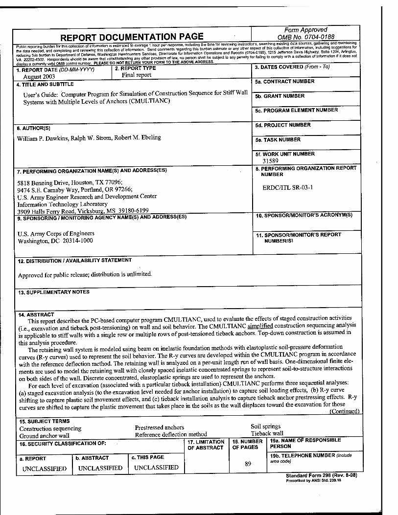
REPORT DOCUMENTATION PAGE Form Approved
0MB No. 0704-0188
display a currently valid 0MB control number. PLEASE DO NOT RETURN YOUR FORM TO THE ABOVE ADDRESS. _ __
1. REPORT DATE (DD-MM-YYYY) August 2003
2. REPORT TYPE Final report
4. TITLE AND SUBTITLE
User's Guide: Computer Program for Simulation of Construction Sequence for Stiff Wall Systems with Multiple Levels of Anchors (CMULTIANC)
6. AUTHOR(S)
William P. Dawkins, Ralph W. Strom, Robert M. Ebeling
7. PERFORMING ORGANIZATION NAME(S) AND ADDRESS(ES)
5818 Benning Drive, Houston, TX 77096; 9474 S.E. Camaby Way, Portland, OR 97266; U.S. Army Engineer Research and Development Center Information Technology Laboratory 3909 Halls Ferry Road, Vicksburg. MS 39180-6199 9. SPONSORING / MONITORING AGENCY NAME(S) AND ADDRESS(ES)
U.S. Army Corps of Engineers Washington, DC 20314-1000
3. DATES COVERED (From - To)
5a. CONTRACT NUMBER
5b. GRANT NUMBER
5c. PROGRAM ELEMENT NUMBER
5d. PROJECT NUMBER
5e. TASK NUMBER
5f. WORK UNIT NUMBER 31589
8. PERFORMING ORGANIZATION REPORT NUMBER
ERDC/ITL SR-03-1
10. SPONSOR/MONITOR'S ACRONYM(S)
11. SPONSOR/MONITOR'S REPORT NUMBERrS)
12. DISTRIBUTION / AVAILABILITY STATEMENT
Approved for public release; distribution is unlimited.
13. SUPPLEMENTARY NOTES
" This report describes the PC-based computer program CMULTIANC, used to evaluate the effects of staged construction activities (i e excavation and tieback post-tensioning) on wall and soil behavior. The CMULTIANC simplified construction sequencmg analysis is applicable to stiff walls with a single row or multiple rows of post-tensioned tieback anchors. Top-down construction is assumed m this analysis procedure. , . ., j x- *•
The retaining wall system is modeled using beam on inelastic foundation methods with elastoplastic soil-pressure detormation curves (R-y curves) used to represent the soil behavior. The R-y curves are developed within the CMULTIANC program in accordance with the reference deflection method. The retaining wall is analyzed on a per-unit length run of wall basis. One-dimensional finite ele- ments are used to model the retaining wall with closely spaced inelastic concentrated springs to represent soil-to-structure interactions on both sides of the wall. Discrete concentrated, elastoplastic springs are used to represent the anchors.
For each level of excavation (associated with a particular tieback installation) CMULTIANC performs three sequential analyses: (a) staged excavation analysis (to the excavation level needed for anchor installation) to capture soil loading effects, (b) R-y curve shifting to capture plastic soil movement effects, and (c) tieback installation analysis to capture tieback anchor prestressing effects. R-y curves are shifted to capture the plastic movement that takes place in the soils as the wall displaces toward the excavation for those
(Continued)
15. SUBJECT TERMS Construction sequencing Groimd anchor wall
Prestressed anchors Reference deflection method
Soil springs Tieback wall
16. SECURITY CLASSIFICATION OF:
a. REPORT
UNCLASSIFIED
b. ABSTRACT
UNCLASSIFIED
c. THIS PAGE
UNCLASSIFIED
17. LIMITATION OF ABSTRACT
18. NUMBER OF PAGES
89
19a. NAME OF RESPONSIBLE PERSON
19b. TELEPHONE NUMBER (include area code)
Standard Form 298 (Rev. 8-98) Prescribed by ANSI Std. 239.18

14. (Concluded)
conditions where actual wall computed displacements exceed active computed displacements. R-y curve shifting is necessary to properly capture soil reloading effects as tieback anchors are post-tensioned and the wall is pulled back into the retained soil.


![Computer Aided Structural Analysis[1]](https://img.pdfslide.us/doc/110x75/577d22ae1a28ab4e1e97fd37/computer-aided-structural-analysis1.jpg)


![[Sowfo.com] AutoCAD Structural Detailing - Formwork Drawings - User's Manual](https://img.pdfslide.us/doc/110x75/577ca4d11a28abea748b478b/sowfocom-autocad-structural-detailing-formwork-drawings-users-manual.jpg)