Computational Topology for Point Data:Betti Numbers ofα-Shapes

Vanessa Robins

Department of Applied Mathematics, Research School of Physical Sciences and Engineering,Australian National University, Canberra ACT 0200.e-mail: vanessa.robins@anu.edu.au

Abstract. The problem considered below is that of determining information about the topology ofa subsetX ⊂ R

n given only a finite point approximation toX. The basic approach is to computetopological properties – such as the number of components and number of holes – at a sequenceof resolutions, and then to extrapolate. Theoretical foundations for taking this limit come fromthe inverse limit systems of shape theory andCech homology. Computer implementations involveconstructions from discrete geometry such as alpha shapes and the minimal spanning tree.

1 Introduction

Two objects have the same topology if they are homeomorphic, i.e. when there is acontinuous transformation from one to the other, with a continuous inverse. This meanstopological properties give a fundamental description of structure, and one that is inde-pendent of geometry. It is clear that objects can have the same topology and completelydifferent geometry (a coffee cup and a donut are archetypal examples). However, theconverse is also true: objects can have very similar geometric properties but a vastly dif-ferent topology – the fractals in Sect. 5.2 are one example. Thus, in order to characterizespatial structures, we need both geometric and topological information.

Much attention has been given to the computation of geometric quantities from data,for example the Minkowski functionals [21, 22] and fractal dimensions [3, 26], but thefield of ‘computational topology’ is relatively new [6]. The earliest work on extractingtopological information from data targeted digital images. For black and white pixelor voxel images there are algorithms for labelling connected components [16], and forcomputing the Euler characteristic [19, 25] (a measure of connectivity that also appearsas the zero-dimensional Minkowski functional). The technique of erosion and dilationis used in conjunction with these algorithms to probe structure at different length scalesin digital images [2].

In this paper we discuss topological properties such as the number of connectedcomponents and number ofk-dimensional holes, i.e., the Betti numbers,βk. The Bettinumbers are related to the Euler characteristic,χ, via the Euler-Poincare formula:

χ = β0 − β1 + β2 − . . .+ βd.

It follows that the Betti numbers give a more detailed description of topological structurethan the Euler characteristic alone. Formal definitions of the Betti numbers are given inSect. 2.

K.R. Mecke, D. Stoyan (Eds.): LNP 600, pp. 261–274, 2002.c© Springer-Verlag Berlin Heidelberg 2002

262 Vanessa Robins

We assume the data are given as a finite point pattern,S ⊂ Rd. To give this finite set

of points some non-trivial topological structure, we must first fatten or coarse-grain theset. This can be achieved, for example, by overlaying a digital mesh and colouring pixelsif they contain data points, or by attaching spheres of radiusα at each point. We focuson the latter objects, called alpha neighbourhoods or alpha parallel bodies, because theyform a more flexible framework.

Once we choose the coarsening method, we have to set an appropriate level ofcoarse-graining. This might be physically motivated, or we may have complete freedomto choose. Without any a priori information, it is helpful to coarse-grain at a sequence ofresolutions. This has the additional advantages of allowing us to detect fractal scaling,and if the data,S, approximate an underlying object,X ⊂ R

d, we can extrapolateinformation about the topology ofX. Theoretical underpinnings of this coarse-grainingand extrapolation are described in Sect. 3.

To compute Betti numbers, we need a discrete complex (e.g., a triangulation) that hasthe same topology as the alpha neighbourhood. One solution comes from Edelsbrunner’salpha shapes [8] and their construction is described in Sect. 4. We use the publiclyavailable alpha shape software [1] to compute Betti numbers of some example data in2D and present the results in Sect. 5.

2 Homology Groups and Betti Numbers

Homology theory is a branch of topology that attempts to distinguish between objectsby constructing algebraic invariants that reflect their connectivity properties. Readersshould be warned that the homology groups do not completely determine the topologyof an object. If two objects have different homology groups, then they certainly havedifferent topologies. The converse, however, does not hold. For example, the setXshown in Fig. 3 has the same homology groups as a circle, but it is not homeomorphicto a circle because of the branch-point where the ‘O’ joins the ‘C’.

In this section, we give a brief outline of the definitions for simplicial homology,following Munkres [24]. The basic building block is anorientedk-simplex, σk, theconvex hull ofk + 1 geometrically independent points,σk = [x0, x1, . . . , xk]. Its ori-entation is defined by an arbitrary but fixed ordering of the vertices. Even permutationsof this ordering give the same orientation and odd permutations reverse it. For example,a 0-simplex is just a point, a1-simplex is a line segment, a2-simplex a triangle, and a3-simplex is a tetrahedron. Asimplicial complex, C, is a collection of oriented simpliceswith the property that the non-empty intersection of two simplices inC must itself be asimplex inC. The set-theoretic union of all simplices fromC, when viewed as a subsetof R

d, is called apolytope. If a subsetX of Rd is homeomorphic to a polytope, we say

X is triangulatedby C.The simplicial complex,C, is given a group structure by defining the addition of

k-simplices in a similar manner to addition in a vector space. The resulting free group iscalled thechain group, Ck. Its elements consist ofk-chains, the sum of a finite numberof orientedk-simplices:ck =

∑i aiσ

ki . The coefficients,ai, are typically integers, but

in general they can be elements of any abelian group,G. In this paper, we use the rationalor real numbers for coefficients since this simplifies the homology group structure (we

Betti Numbers ofα-Shapes 263

c

a b

e

c

a b

0

e

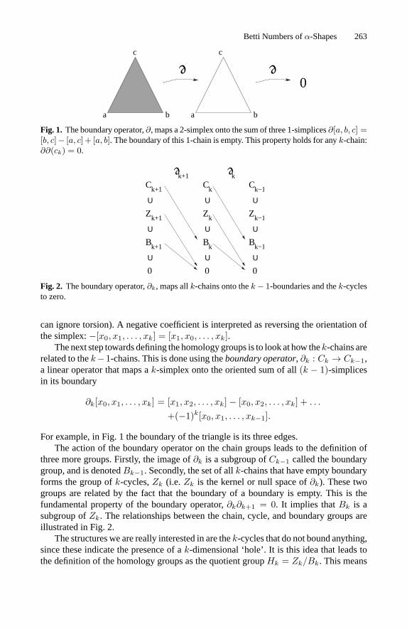
Fig. 1. The boundary operator,∂, maps a 2-simplex onto the sum of three 1-simplices∂[a, b, c] =[b, c] − [a, c] + [a, b]. The boundary of this 1-chain is empty. This property holds for anyk-chain:∂∂(ck) = 0.

Ck−1

Bk−1

Zk−1

Ck

Zk

Bk

e

k

U

U

U

0

U

U

U

0

B

Z

Ck+1

k+1

k+1

e

k+1

0

U

U

U

Fig. 2. The boundary operator,∂k, maps allk-chains onto thek − 1-boundaries and thek-cyclesto zero.

can ignore torsion). A negative coefficient is interpreted as reversing the orientation ofthe simplex:−[x0, x1, . . . , xk] = [x1, x0, . . . , xk].

The next step towards defining the homology groups is to look at how thek-chains arerelated to thek−1-chains. This is done using theboundary operator, ∂k : Ck → Ck−1,a linear operator that maps ak-simplex onto the oriented sum of all(k − 1)-simplicesin its boundary

∂k[x0, x1, . . . , xk] = [x1, x2, . . . , xk] − [x0, x2, . . . , xk] + . . .+(−1)k[x0, x1, . . . , xk−1].

For example, in Fig. 1 the boundary of the triangle is its three edges.The action of the boundary operator on the chain groups leads to the definition of

three more groups. Firstly, the image of∂k is a subgroup ofCk−1 called the boundarygroup, and is denotedBk−1. Secondly, the set of allk-chains that have empty boundaryforms the group ofk-cycles,Zk (i.e.Zk is the kernel or null space of∂k). These twogroups are related by the fact that the boundary of a boundary is empty. This is thefundamental property of the boundary operator,∂k∂k+1 = 0. It implies thatBk is asubgroup ofZk. The relationships between the chain, cycle, and boundary groups areillustrated in Fig. 2.

The structures we are really interested in are thek-cycles that do not bound anything,since these indicate the presence of ak-dimensional ‘hole’. It is this idea that leads tothe definition of the homology groups as the quotient groupHk = Zk/Bk. This means

264 Vanessa Robins

X · · · Xλi−→ Xα

Cech homology · · · Hk(Xλ) i∗−→ Hk(Xα)

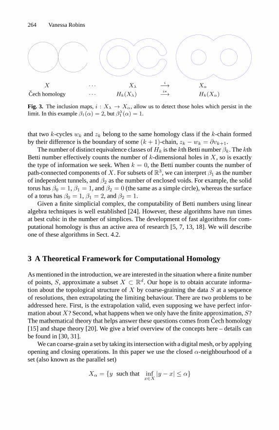
Fig. 3. The inclusion maps,i : Xλ → Xα, allow us to detect those holes which persist in thelimit. In this exampleβ1(α) = 2, butβλ

1 (α) = 1.

that twok-cycleswk andzk belong to the same homology class if thek-chain formedby their difference is the boundary of some(k + 1)-chain,zk − wk = ∂vk+1.

The number of distinct equivalence classes ofHk is thekth Betti numberβk. ThekthBetti number effectively counts the number ofk-dimensional holes inX, so is exactlythe type of information we seek. Whenk = 0, the Betti number counts the number ofpath-connected components ofX. For subsets ofR3, we can interpretβ1 as the numberof independent tunnels, andβ2 as the number of enclosed voids. For example, the solidtorus hasβ0 = 1, β1 = 1, andβ2 = 0 (the same as a simple circle), whereas the surfaceof a torus hasβ0 = 1, β1 = 2, andβ2 = 1.

Given a finite simplicial complex, the computability of Betti numbers using linearalgebra techniques is well established [24]. However, these algorithms have run timesat best cubic in the number of simplices. The development of fast algorithms for com-putational homology is thus an active area of research [5, 7, 13, 18]. We will describeone of these algorithms in Sect. 4.2.

3 A Theoretical Framework for Computational Homology

As mentioned in the introduction, we are interested in the situation where a finite numberof points,S, approximate a subsetX ⊂ R

d. Our hope is to obtain accurate informa-tion about the topological structure ofX by coarse-graining the dataS at a sequenceof resolutions, then extrapolating the limiting behaviour. There are two problems to beaddressed here. First, is the extrapolation valid, even supposing we have perfect infor-mation aboutX? Second, what happens when we only have the finite approximation,S?The mathematical theory that helps answer these questions comes fromCech homology[15] and shape theory [20]. We give a brief overview of the concepts here – details canbe found in [30, 31].

We can coarse-grain a set by taking its intersection with a digital mesh, or by applyingopening and closing operations. In this paper we use the closedα-neighbourhood of aset (also known as the parallel set)

Xα = {y such that infx∈X

|y − x| ≤ α}

Betti Numbers ofα-Shapes 265

where|.| is the Euclidean metric onRd. The following theory is easily adapted to thecase of digital meshes and other standard methods of coarse-graining.

Our question now is: for what spaces do the Betti numbers of theα-neighbourhoods,Xα, converge to those ofX? That is, doesβk(Xα) → βk(X) asα → 0? For thenumber of components,β0(Xα), this holds for any compact set (i.e. closed and boundedsubsets ofRd) [15, 28]. This restriction to compact sets is not unreasonable, since weare primarily interested in objects that are well approximated on a computer by a finitenumber of points.

Higher-order Betti numbers present a more subtle problem, because fattening a set toitsα-neighbourhood can introduce holes, as illustrated in Fig. 3, and also remove holesby filling them in. Mathematically, this problem is resolved by incorporating informationabout how a smaller neighbourhood maps inside a larger one. This leads to the definitionof persistent Betti number. Suppose0 ≤ λ < α, so thatXλ ⊂ Xα. The inclusion mapi : Xλ → Xα induces a homomorphism on the homology groups,i∗ : Hk(λ) → Hk(α).We define theλ-persistent Betti number,βλ

k (α), to be the rank ofi∗, i.e. the number ofnon-equivalent, non-boundingk-cycles inHk(α) that are the image of ak-cycle fromHk(λ). This leads to the formula

βλk (α) = rank[Zk(λ)] − rank[i∗(Zk(λ)) ∩Bk(α)] (1)

Geometrically,βλk (α) is the number of holes inXλ that do not get filled in by taking a

fatter neighbourhood,Xα.Cycles inXα that genuinely come from a cycle inX are the 0-persistent Betti

numbers,β0k(α) ≤ βλ

k (α) for all 0 ≤ λ ≤ α. From the continuity ofCech homology,we know that the 0-persistent Betti numbers of theα-neighbourhoods converge to thoseof the original space:β0

k(α) → βk(X), whenX is compact. Thus, to find the regularBetti number of X,βk(X), from the persistent Betti numbersβλ

k (α), we must first fix asequence ofα-values and letλ → 0 to get the limitsβλ

k (αn) → β0k(αn). Then we can

find βk(X) as the limit of this sequence: forαn → 0, β0k(αn) → βk(X).

The second problem we must address concerns the relationship between the neigh-bourhoods of the data,Sα, and those of the set they approximate,Xα. Intuitivelyspeaking, the idea is that if the data and the underlying set are “close” then theirα-neighbourhoods should have similar topological properties, providedα is sufficientlylarge. We measure the distance between the data,S, and the underlying space,X, usingthe Hausdorff metric on compact sets. This is defined as

dH(S,X) = min{α | X ⊂ Sα andS ⊂ Xα}. (2)

If ρ = dH(S,X), it follows thatSα ⊂ Xα+ρ andXα ⊂ Sα+ρ for all α > 0. Theseinclusions allow us to derive a number of inequalities relating the persistent Betti numbersof X to those ofS [31]. For example, we have that forα > ρ, β0

k(Xα+ρ) ≤ βρk(Sα)

andβα−ρk (Sα+ρ) ≤ βk(Xα). For the number of connected components, the persistent

Betti number is the same as the regular Betti number and we find thatβ0(Sα−ρ) ≥β0(Xα) ≥ β0(Sα+ρ). We refer toρ as thecutoff resolution, since we cannot hope to getvalid topological information aboutX from Sα unlessα > ρ.

266 Vanessa Robins

4 Computer Implementation

We now describe some algorithms for computing Betti numbers from scattered point dataat a sequence ofα-values. We begin with the simple problem of counting the connectedcomponents ofSα.

Fig. 4. The MST of104 points on a Cantor set, and a close up of a small region.

4.1 Connected Components

For scattered point data,S ⊂ Rd, the Euclidean minimal spanning tree (MST) encodes

all the relevant information about connected components at all resolutions [29]. Recallthat the MST is a tree (i.e. a graph with no cycles) that passes through every point in sucha way as to minimize the total length. There are a number of algorithms for constructingthe MST; the most easily implemented one is due Prim [4, 27]. This starts with anypoint and joins its nearest neighbour to create an initial subtree. The algorithm proceedsincrementally by adding the point which is closest to the existing subtree, finishing whenall points have been added. The computational complexity is quadratic in the number ofdata points.

The property of connecting closest points gives the MST a natural correspondencewith the connected components of theα-neighbourhood,Sα, [29]. In fact the numberof components,β0(α), is just one more than the number of MST edges that are longerthan2α:

β0(α) = 1 + #{MST edges> 2α}. (3)

Note that we need only build the MST once to get component information at all scales.

4.2 Alpha Shapes and Homology

We now want to compute higher-order Betti numbers of theα-neighbourhoodsSα fora sequence ofα values. This requires a sequence of simplicial complexes that reflectthe topology of theα-neighbourhoods. An elegant solution to this problem comes fromalpha shapes - a construction based on the Voronoi diagram and its dual, the Delaunaytriangulation. Alpha shapes were defined by Edelsbrunneret al. for finite sets of points

Betti Numbers ofα-Shapes 267

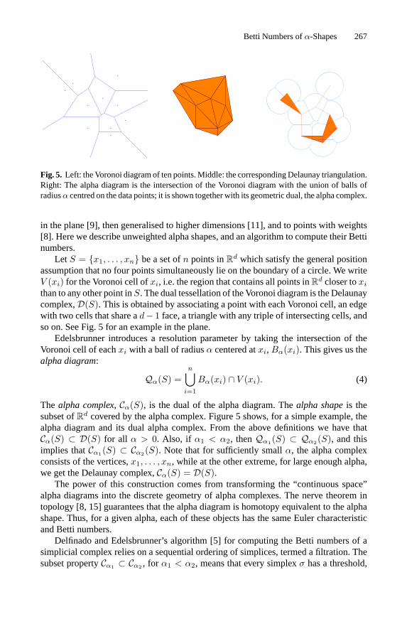
Fig. 5. Left: the Voronoi diagram of ten points. Middle: the corresponding Delaunay triangulation.Right: The alpha diagram is the intersection of the Voronoi diagram with the union of balls ofradiusα centred on the data points; it is shown together with its geometric dual, the alpha complex.

in the plane [9], then generalised to higher dimensions [11], and to points with weights[8]. Here we describe unweighted alpha shapes, and an algorithm to compute their Bettinumbers.

Let S = {x1, . . . , xn} be a set ofn points inRd which satisfy the general position

assumption that no four points simultaneously lie on the boundary of a circle. We writeV (xi) for the Voronoi cell ofxi, i.e. the region that contains all points inR

d closer toxi

than to any other point inS. The dual tessellation of the Voronoi diagram is the Delaunaycomplex,D(S). This is obtained by associating a point with each Voronoi cell, an edgewith two cells that share ad− 1 face, a triangle with any triple of intersecting cells, andso on. See Fig. 5 for an example in the plane.

Edelsbrunner introduces a resolution parameter by taking the intersection of theVoronoi cell of eachxi with a ball of radiusα centered atxi,Bα(xi). This gives us thealpha diagram:

Qα(S) =n⋃

i=1

Bα(xi) ∩ V (xi). (4)

The alpha complex, Cα(S), is the dual of the alpha diagram. Thealpha shapeis thesubset ofRd covered by the alpha complex. Figure 5 shows, for a simple example, thealpha diagram and its dual alpha complex. From the above definitions we have thatCα(S) ⊂ D(S) for all α > 0. Also, if α1 < α2, thenQα1(S) ⊂ Qα2(S), and thisimplies thatCα1(S) ⊂ Cα2(S). Note that for sufficiently smallα, the alpha complexconsists of the vertices,x1, . . . , xn, while at the other extreme, for large enough alpha,we get the Delaunay complex,Cα(S) = D(S).

The power of this construction comes from transforming the “continuous space”alpha diagrams into the discrete geometry of alpha complexes. The nerve theorem intopology [8, 15] guarantees that the alpha diagram is homotopy equivalent to the alphashape. Thus, for a given alpha, each of these objects has the same Euler characteristicand Betti numbers.

Delfinado and Edelsbrunner’s algorithm [5] for computing the Betti numbers of asimplicial complex relies on a sequential ordering of simplices, termed a filtration. Thesubset propertyCα1 ⊂ Cα2 , for α1 < α2, means that every simplexσ has a threshold,

268 Vanessa Robins

αc(σ), such thatσ ∈ Cα for all α > αc(σ). The filtration orders the simplices accordingto their thresholds. Note that two simplices may have the same threshold, and in thissituation they are ordered by adding the lower dimensional simplices first. The Bettinumbers are computed incrementally as each simplex is added to the complex. Thisprocess depends on a test to determine whether the new simplex belongs to ak-cycleof the new complex. There are efficient algorithms for testing 1-cycles, and homology-cohomology duality theorems transform the(d − 1)-cycles into 1-cocycles that areequally easy to test for. However, there is no fast test for otherk-cycles, so Delfinadoand Edelsbrunner’s algorithm applies only to subcomplexes ofR

2 or R3.

The computational complexity involved in building the Delaunay triangulation inR3

is quadratic in the number of points, and the incremental algorithm for computing Bettinumbers is barely super-linear in the number of simplices. The NCSA ftp site providessoftware that implements the above alpha shape constructions inR

2 andR3 [1]. The

Betti number data for the examples in the following section were generated using thissoftware.

The numerical computation of persistent Betti numbers is possible using linear al-gebra techniques but is not yet implemented. Recently, Edelsbrunner [10] has made asimilar definition of persistence specific to alpha shapes and has developed an incremen-tal algorithm for this quantity.

5 Example Data

The random point clouds we study tend to have three regimes determined by the cutoffresolutionρ discussed in Sect. 3. Forα� ρwe recover the coarse-scale topology of theapproximated regionX. At the other extreme,α� ρwe see purely the statistical effectsof a point process. Whenα is on the same order asρ, there is transitional behaviour asthe finite data effects begin to dominate the underlying topological structure.

In the following two subsections we analyse the Betti numbers for data from abinomial point process and a family of self-similar fractals. For a finite domain, the coarsescale topology of the binomial point pattern is extremely simple, so the interesting Bettinumber behaviour occurs only forα ≤ ρ. The fractal examples have identical fractaldimension, but greatly differing topological structure. The Betti number data at coarseresolutions distinguishes between the different topological types. Forα < ρ, however,the fractals show essentially the same behaviour, presumably dictated by the iteratedfunction system technique of generating the data points.

5.1 Binomial Point Process

We begin by analysingN points that are randomly distributed in the unit square accord-ing to a binomial point process. The coordinates of each point are assigned using theuniform distribution on[0, 1] and the point pattern therefore constitutes a finite-domainapproximation to a Poisson process with intensityλ = N/1. We describe the behaviourof a typical single realisation ofN points, and then present results from a numericalinvestigation of the mean values ofβ0 andβ1 as functions of the radiusα.

Betti Numbers ofα-Shapes 269

10−4

10−3

10−2

10−1

100

100

101

102

103

104

α

1β

β0

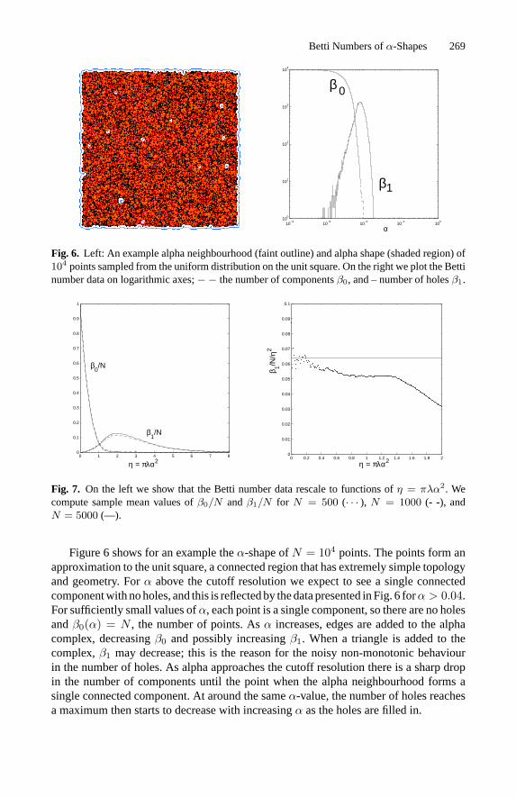
Fig. 6. Left: An example alpha neighbourhood (faint outline) and alpha shape (shaded region) of104 points sampled from the uniform distribution on the unit square. On the right we plot the Bettinumber data on logarithmic axes;− − the number of componentsβ0, and – number of holesβ1.

0 1 2 3 4 5 6 7 80

0.1

0.2

0.3

0.4

0.5

0.6

0.7

0.8

0.9

1

η = πλα2

β0/N

β1/N

0 0.2 0.4 0.6 0.8 1 1.2 1.4 1.6 1.8 20

0.01

0.02

0.03

0.04

0.05

0.06

0.07

0.08

0.09

0.1

η = πλα2

β 1/N/η

2

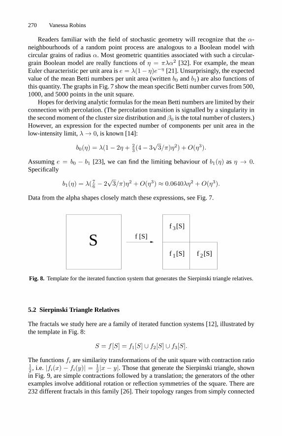
Fig. 7. On the left we show that the Betti number data rescale to functions ofη = πλα2. Wecompute sample mean values ofβ0/N andβ1/N for N = 500 (· · · ), N = 1000 (- -), andN = 5000 (—).

Figure 6 shows for an example theα-shape ofN = 104 points. The points form anapproximation to the unit square, a connected region that has extremely simple topologyand geometry. Forα above the cutoff resolution we expect to see a single connectedcomponent with no holes, and this is reflected by the data presented in Fig. 6 forα > 0.04.For sufficiently small values ofα, each point is a single component, so there are no holesandβ0(α) = N , the number of points. Asα increases, edges are added to the alphacomplex, decreasingβ0 and possibly increasingβ1. When a triangle is added to thecomplex,β1 may decrease; this is the reason for the noisy non-monotonic behaviourin the number of holes. As alpha approaches the cutoff resolution there is a sharp dropin the number of components until the point when the alpha neighbourhood forms asingle connected component. At around the sameα-value, the number of holes reachesa maximum then starts to decrease with increasingα as the holes are filled in.

270 Vanessa Robins

Readers familiar with the field of stochastic geometry will recognize that theα-neighbourhoods of a random point process are analogous to a Boolean model withcircular grains of radiusα. Most geometric quantities associated with such a circular-grain Boolean model are really functions ofη = πλα2 [32]. For example, the meanEuler characteristic per unit area ise = λ(1 − η)e−η [21]. Unsurprisingly, the expectedvalue of the mean Betti numbers per unit area (writtenb0 andb1) are also functions ofthis quantity. The graphs in Fig. 7 show the mean specific Betti number curves from 500,1000, and 5000 points in the unit square.

Hopes for deriving analytic formulas for the mean Betti numbers are limited by theirconnection with percolation. (The percolation transition is signalled by a singularity inthe second moment of the cluster size distribution andβ0 is the total number of clusters.)However, an expression for the expected number of components per unit area in thelow-intensity limit,λ→ 0, is known [14]:

b0(η) = λ(1 − 2η + 23 (4 − 3

√3/π)η2) +O(η3).

Assuminge = b0 − b1 [23], we can find the limiting behaviour ofb1(η) asη → 0.Specifically

b1(η) = λ( 76 − 2

√3/π)η2 +O(η3) ≈ 0.0640λη2 +O(η3).

Data from the alpha shapes closely match these expressions, see Fig. 7.

S f [S]

f

f f 21

3[S]

[S] [S]

Fig. 8. Template for the iterated function system that generates the Sierpinski triangle relatives.

5.2 Sierpinski Triangle Relatives

The fractals we study here are a family of iterated function systems [12], illustrated bythe template in Fig. 8:

S = f [S] = f1[S] ∪ f2[S] ∪ f3[S].

The functionsfi are similarity transformations of the unit square with contraction ratio12 , i.e. |fi(x) − fi(y)| = 1

2 |x − y|. Those that generate the Sierpinski triangle, shownin Fig. 9, are simple contractions followed by a translation; the generators of the otherexamples involve additional rotation or reflection symmetries of the square. There are232 different fractals in this family [26]. Their topology ranges from simply connected

Betti Numbers ofα-Shapes 271

10−4

10−3

10−2

10−1

100

100

101

102

103

104

α

β0

1β

10−4

10−3

10−2

10−1

100

100

101

102

103

104

α

1β

β0

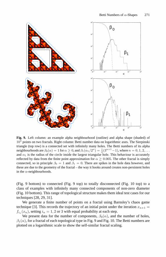
Fig. 9. Left column: an example alpha neighbourhood (outline) and alpha shape (shaded) of104 points on two fractals. Right column: Betti number data on logarithmic axes. The Sierpinskitriangle (top row) is a connected set with infinitely many holes. The Betti numbers of its alphaneighbourhoods areβ0(α) = 1 for α ≥ 0, andβ1(α1/2n) = 1

2 (3n+1−1), wheren = 0, 1, 2, . . .andα1 is the radius of the circle inside the largest triangular hole. This behaviour is accuratelyreflected by data from the finite point approximation forα ≥ 0.005. The other fractal is simplyconnected, so in principleβ0 = 1 andβ1 = 0. There are spikes in the hole data however, andthese are due to the geometry of the fractal – the way it hooks around creates non-persistent holesin theα-neighbourhoods.

(Fig. 9 bottom) to connected (Fig. 9 top) to totally disconnected (Fig. 10 top) to aclass of examples with infinitely many connected components of non-zero diameter(Fig. 10 bottom). This range of topological structure makes them ideal test cases for ourtechniques [28, 29, 31].

We generate a finite number of points on a fractal using Barnsley’s chaos gametechnique [3]. This records the trajectory of an initial point under the iterationxn+1 =fin(xn), settingin = 1, 2 or 3 with equal probability at each step.

We present data for the number of components,β0(α), and the number of holes,β1(α), for a fractal of each topological type in Fig. 9 and Fig. 10. The Betti numbers areplotted on a logarithmic scale to show the self-similar fractal scaling.

272 Vanessa Robins

10−4

10−3

10−2

10−1

100

100

101

102

103

104

α

β0

1β

10−4

10−3

10−2

10−1

100

100

101

102

103

104

α

1β

β0

Fig. 10. Left column: an example alpha neighbourhood (outline) and alpha shape (shaded) of104

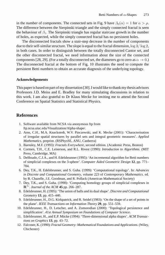
points on two fractals. Right column: Betti number data on logarithmic axes. The upper fractal isa Cantor set so it is totally disconnected and perfect. We find [28]β0(α0/2n) → 3n asn → ∞(whereα0 is the width of the largest gap) andβ1(α) = 0. Although topologically the Cantor setdoes not contain any holes, the graph ofβ1(α) has regularly spaced spikes. The reason for these isseen in theα-neighbourhood picture. The edges bridging the gaps cause holes in the triangulationthat disappear for slightly smaller values ofα when the edges are removed from the alpha shape.The lower fractal is disconnected, and consists of infinitely many line segments. Again, there areno topological holes in this fractal. It is the geometry of the set, i.e., the arrangement of the linesegments in the plane, that creates holes in theα-neighbourhoods. Again,β0(α0/2n) → 3n. Theregular Betti number shows fractal growthβ1(α1/2n) = 3n, while the 0-persistent Betti numbersareβ0

1(α) = 0.

Each of these fractals has a cutoff resolutionρ ≈ 0.005. Forα < ρ, the behaviour ofthe Betti number data is quantitatively similar for each fractal and qualitatively similar tothat of the point process in Sect. 5.1. Preliminary analysis suggests that for each of thesefractals, the Betti numbers are really functions of the rescaled quantityη = πNαdf ,wheredf = log 3/ log 2 is the fractal dimension. In particular we findβ0(η)/N → 1−ηandβ1(η) = O(ηdf ) asη → 0.

It is in the regionα > ρ that we see the effects of the different topology of eachfractal. The difference between the connected and disconnected fractals shows up clearly

Betti Numbers ofα-Shapes 273

in the number of components. The connected sets in Fig. 9 haveβ0(α) = 1 for α > ρ.The difference between the Sierpinski triangle and the simply connected fractal is seenthe behaviour ofβ1. The Sierpinski triangle has regular staircase growth in the numberof holes, as expected, while the simply connected fractal has no persistent holes.

The disconnected fractals show a stair-step decrease in the number of componentsdue to their self-similar structure. The slope is equal to the fractal dimension,log 3/ log 2,in both cases. In order to distinguish between the totally disconnected Cantor set, andthe other disconnected fractal, we need information about the size of the connectedcomponents [28, 29]. (For a totally disconnected set, the diameters go to zero asα→ 0.)The disconnected fractal at the bottom of Fig. 10 illustrates the need to compute thepersistent Betti numbers to obtain an accurate diagnosis of the underlying topology.

Acknowledgements

This paper is based on part of my dissertation [30]. I would like to thank my thesis advisorsProfessors J.D. Meiss and E. Bradley for many stimulating discussions in relation tothis work. I am also grateful to Dr Klaus Mecke for inviting me to attend the SecondConference on Spatial Statistics and Statistical Physics.

References

1. Software available from NCSA via anonymous ftp fromftp.ncsa.uiuc.edu/Visualization/Alpha-shape/.

2. Arns, C.H., M.A. Knackstedt, W.V. Pinczewski, and K. Mecke (2001): ‘Characterisationof irregular spatial structures by parallel sets and integral geometric measures’.AppliedMathematics, preprint. (RSPhysSE, ANU, Canberra)

3. Barnsley, M.F. (1993):Fractals Everywhere, second edition. (Academic Press, Boston)4. Cormen, T.H., C.E. Leiserson, and R.L. Rivest (1990):Introduction to Algorithms. (MIT

Press, Cambridge, MA)5. Delfinado, C.J.A., and H. Edelsbrunner (1995): ‘An incremental algorithm for Betti numbers

of simplicial complexes on the 3-sphere’.Computer Aided Geometric Design12, pp. 771–784.

6. Dey, T.K., H. Edelsbrunner, and S. Guha. (1999): ‘Computational topology’. In:Advancesin Discrete and Computational Geometry, volume 223 ofContemporary Mathematics. ed.by B. Chazelle, J.E. Goodman, and R. Pollack (American Mathematical Society)

7. Dey, T.K., and S. Guha. (1998): ‘Computing homology groups of simplicial complexes inR3’. Journal of the ACM45pp. 266–287.

8. Edelsbrunner, H. (1995): ‘The union of balls and its dual shape’.Discrete andComputationalGeometry13, pp. 415–440.

9. Edelsbrunner, H., D.G. Kirkpatrick, and R. Seidel (1983): ‘On the shape of a set of points inthe plane’.IEEE Transactions on Information Theory29, pp. 551–559.

10. Edelsbrunner, H., D. Letscher, and A. Zomorodian (2000): ‘Topological persistence andsimplification’.41st Annual Symposium on Foundations of Computer Science.

11. Edelsbrunner, H., and E.P. Mucke (1994): ‘Three-dimensional alpha shapes’.ACM Transac-tions on Graphics13, pp. 43–72.

12. Falconer, K. (1990):FractalGeometry:Mathematical Foundations andApplications. (Wiley,Chichester)

274 Vanessa Robins

13. Friedman, J. (1998): ‘Computing Betti numbers via combinatorial Laplacians’.Algorithmica21, pp. 331–346.

14. Hall, P. (1988):Introduction to the Theory of Coverage Processes. (Wiley, Chichester)15. Hocking, J.G., and G.S. Young (1961):Topology. (Addison-Wesley)16. Hoshen, J. and Kopelman, R. (1976): ‘Percolation and cluster distribution. I. Cluster multiple

labeling technique and critical concentration algorithm’.Physical Review B14, pp. 3438–3445.

17. Hutchinson, J.E. (1981): ‘Fractals and self similarity’.IndianaUniversityMathematics Jour-nal 30, pp. 713–747.

18. Kalies, W.D., K. Mischaikow, and G. Watson (1999): ‘Cubical approximation and computa-tion of homology’.Banach Center Publications47, pp. 115–131.

19. Lee, C.-N., T. Posten, and A. Rosenfeld (1991): ‘Winding and Euler numbers for 2D and 3Ddigital images’.CVGIP: Graphical Models and Image Processing53, pp. 522-537.

20. Mardesic, S. and J. Segal (1982):Shape Theory. (North-Holland)21. Mecke, K. (1998): ‘Integral geometry and statistical physics’.International Journal of Mod-

ern Physics B12, pp. 861–899.22. Mecke, K. and D. Stoyan (Eds.) (2000):Statistical Physics and Spatial Statistics – The Art of

Analyzing and Modeling Spatial Structures and Pattern FormationLecture Notes in Physics554(Springer-Verlag, Berlin)

23. Mecke, J., and Stoyan, D. (2001): ‘The specific connectivity number of random networks’.Advances in Applied Probability33, pp. 576–583.

24. Munkres, J.R. (1984):Elements of Algebraic Topology. (Benjamin Cummings)25. Nagel, W., J. Ohser, and K. Pischang (2000): ‘An integral-geometric approach for the Euler-

Poincare characteristic of spatial images’.Journal of Microscopy198, pp. 54–62.26. Peitgen, H.-O., S. Jurgens, and D. Saupe. (1992):Chaos and Fractals: New Frontiers of

Science. (Springer-Verlag, Berlin)27. Prim, R.S. (1957): ‘Shortest connection networks and some generalizations’.TheBell System

Technical JournalNovember 1957, pp. 1389–1401.28. Robins, V., J.D. Meiss, and E. Bradley (1998): ‘Computing connectedness: An exercise in

computational topology’.Nonlinearity11, pp. 913–922.29. Robins, V., J.D. Meiss, and E. Bradley (2000): ‘Computing connectedness: Disconnectedness

and discreteness’.Physica D139, pp. 276–300.30. Robins, V. (2000):Computational topology at multiple resolutions. PhD Thesis, Department

of Applied Mathematics, University of Colorado, Boulder.31. Robins, V. (1999): ‘Towards computing homology from finite approximations’.Topology

Proceedings24, pp. 503–532.32. Stoyan, D., W.S. Kendall, and J. Mecke (1987):Stochastic Geometry and its Applications.

(Wiley, Chichester)