Chapter 3

Computing Homology

3.1 Intr oduction

Wenow turnourattentionto themoredifficult problemof deducingthehomologyof acompactmetric spacefrom a finite amountof data. The homologygroupsof a spacecharacterizethenumberand type of holes in that spaceand thereforegive a fundamentaldescriptionof itsstructure. This type of information is used,for example, in understandingthe structureofattractorsfrom embeddedtime seriesdata[58, 60], or for determiningsimilarities betweenproteinsin molecularbiology [13].

Thecomputabilityof homologygroupsfrom agiventriangulationis well-known andtheal-gorithmusessimplelinearalgebra[61]. Thisalgorithmhasextremelypoornumericalbehavior,however, sothestudyof computationalhomologyremainsanactive areaof research.In manyapplicationsknowledgeof theentiregroupstructureis unnecessary— all that is neededis therankof thehomologygroup,i.e.,theBetti number. Thisinformationcanbecomputedindirectlyfrom a triangulation;many algorithmsexist [11, 14, 26, 37]. Theextractionof homologyfromdatainvolvestheadditionalproblemof generatinga triangulationor otherregularcell-complexthat reflectsthetopologyof theunderlyingspace.Therearemany differentapproachesto this[18, 37, 60].

Our goal is to developcomputationaltechniquesthatallow usto extrapolatethehomologyof an underlyingcompactspace,

�, given only a finite approximation,� . We assumethat �

approximates�

in a metricsense,i.e., thatevery point of � is within distance� of�

andviceversa.As in Chapter2, thebasictrick is to coarse-grainthedataat a sequenceof resolutionsthattendto zero.Of course,theextrapolationwill alwaysbeconstrainedby theaccuracy of thedata— this is measuredby � , thecutoff resolution.We modelthecoarse-grainingof a set,

�,

by closed� -neighborhoods:1 ������� �������������� �����Ourmaincontribution to theliteratureoncomputationalhomologyis soundmathematicalfoun-dationsfor relating the homologyof the � -neighborhoodsof � to the homologyof

�. Our

multiresolutionapproachhastheadditionaladvantageof beingapplicableto fractalsets.We begin this chapterwith anoverview of the relevantconceptsfrom homologytheoryin

Section3.2. Thesectionstartsby describingsimplicial homologytheory. This theoryis basedon finite triangulationsso is readily adaptedto computerimplementation.Fractalsetsdo not

1This is a differentcoarse-grainingprocedureto that in Chapter2 — theresolutionparameterthereis relatedtothedistancebetweenpoints.A setis � -connectedin thesenseof Chapter2 if its � �"! -neighborhoodis connected.

39

have finite triangulations,soa moregeneralhomologytheoryis needed.Theappropriatefor-mulationis Cechhomology. Thebasisof Cechhomologyis aninversesystemof finite triangu-lationsthatapproximateaspace.This ideais extendedby shapetheorywhichconsidersinversesystemsof approximatingspacesin amoregeneralclass.Oursequenceof � -neighborhoodsfitsthis framework.

Thecentralresultsof thischapteraregivenin Section3.3.Thissectiondescribestheinversesystemof � -neighborhoodsof

�andthecorrespondinginversesystemsof homologygroups.

We would like to quantify the topologicalstructureby computingBetti numbersasfunctionsof � . Thereis a problemwith this however, sincethe � -neighborhood

���canhave holesthat

do not exist in�

. We resolve this problemby introducing the conceptof persistentBettinumber, which countsthe numberof holesin

���that correspondto a hole in

�. When

�hasfractalstructure,it is possibleto seeunboundedgrowth in thepersistentBetti numbersas�$#&% . We characterizethis growth by assumingan asymptoticpower law. The next part ofthis sectionderivesformal relationshipsbetweenthe � -neighborhoodsof

�anda finite point-

set approximation. For the finite approximations,we show that it is possibleto reducethecomputationof � -persistentBetti numbersto linearalgebra.

In Section3.4, we turn to the practicalproblemof how to implementtheseideascom-putationally. As mentionedabove, therearea numberof existing approachesfor generatingtriangulationsand computingBetti numbers. The one that is closestto our needsis due toEdelsbrunneret al. [11, 18]. Their algorithmsarebasedon subcomplexesof theDelaunaytri-angulationcalledalphashapes.We describetheir approachin somedetail sincewe usetheNCSA implementationof thesealgorithmsto generatedatain Section3.5.Wealsogiveabriefoverview of someothercomputationalhomologyalgorithms. In thefinal part of this section,we outlineamultiresolutionapproachto computationalhomologythatmaybeamoreefficientimplementationof our ideas.

We usethe Sierpinskitriangle relatives as testexamplesagainin Section3.5. Sincewehave not yet implementedalgorithmsfor computingthepersistentBetti numbers,we give datafor theregularBetti numbers.ThisdistinguishesbetweentheconnectedSierpinskitriangleandthesimplyconnectedrelative. TheexamplesdemonstratethattheregularBetti numberscanbemisleadingandthat thepersistentBetti numbersarenecessaryfor a propercharacterizationoftheunderlyingtopology.

Thematerialin Sections3.3–3.5is publishedin [69].

3.2 An overview of homologytheory

Homologytheoryis abranchof algebraictopologythatattemptsto distinguishbetweenspacesby constructingalgebraicinvariantsthat reflect the connectivity propertiesof the space.Thefield hasit originsin thework of Poincare. In Section3.2.1we review thebasicdefinitionsforsimplicial homology— a theorybasedon triangulationsof spaces.Simplicial homologylendsitself to computationalimplementationbecausetriangulationsof dataarecommonnumericalconstructionsand thereis a well definedalgorithm for computinghomologygroupsfrom agiventriangulation.Fractalstypically requireinfinitely many simplicesin their triangulations.This meansthegroupsassociatedwith a fractalshouldalsobeinfinite, but this is not possiblewith simplicial homology. A differentapproachis needed,therefore,to describespaceswithinfinitely detailedstructure. The appropriateformulation of limit for this situationis givenby the machineryof inversesystems,which we describein Section3.2.3. An inverselimitsystemis thenusedto defineCechhomologyin Section3.2.4. We alsogive a brief outlineof

40

a b

c

a b

c

[abc] = [bca] = [cab]σ −σ

[bac] = [acb]=[cba]

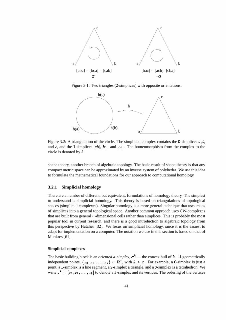
Figure3.1: Two triangles(2-simplices)with oppositeorientations.

. .

.

h(a) h(b)

h(c)

a b

c

h

Figure3.2: A triangulationof thecircle. Thesimplicial complex containsthe % -simplices' �)(,

and * , andthe + -simplices , ' ()-.� , ( * - , and , *�' - . The homeomorphismfrom the complex to thecircle is denotedby / .

shapetheory, anotherbranchof algebraictopology. Thebasicresultof shapetheoryis thatanycompactmetricspacecanbeapproximatedby aninversesystemof polyhedra.Weusethis ideato formulatethemathematicalfoundationsfor ourapproachto computationalhomology.

3.2.1 Simplicial homology

Thereareanumberof different,but equivalent,formulationsof homologytheory. Thesimplestto understandis simplicial homology. This theory is basedon triangulationsof topologicalspaces(simplicial complexes). Singularhomologyis a moregeneraltechniquethatusesmapsof simplicesinto a generaltopologicalspace.AnothercommonapproachusesCW-complexesthatarebuilt from general0 -dimensionalcellsratherthansimplices.This is probablythemostpopulartool in currentresearch,andthereis a good introductionto algebraictopologyfromthis perspective by Hatcher[32]. We focuson simplicial homology, sinceit is the easiesttoadaptfor implementationonacomputer. Thenotationweusein thissectionis basedon thatofMunkres[61].

Simplicial complexes

Thebasicbuilding block is anoriented1 -simplex, 243 — theconvex hull of 1657+ geometricallyindependentpoints,

���89�:<;=� �>�>� �: 3 �@?BA�C , with 1 � 0 . For example,a % -simplex is just apoint,a + -simplex is aline segment,a D -simplex atriangle,anda E -simplex is atetrahedron.Wewrite 2 3 � , �8��:<;=� �>�>� �: 3 - to denotea 1 -simplex andits vertices.Theorderingof thevertices

41

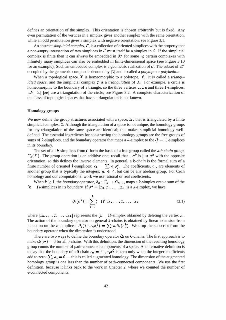
definesan orientationof the simplex. This orientationis chosenarbitrarily but is fixed. Anyevenpermutationof theverticesin a simplex givesanothersimplex with thesameorientation,while anoddpermutationgivesa simplex with negative orientation;seeFigure3.1.

An abstractsimplicialcomplex, F , is acollectionof orientedsimpliceswith thepropertythata non-emptyintersectionof two simplicesin F mustitself bea simplex in F . If thesimplicialcomplex is finite thenit canalwaysbe embeddedin AGC for some 0 ; certaincomplexeswithinfinitely many simplicescanalsobe embeddedin finite-dimensionalspace(seeFigure3.10for anexample).Suchanembeddedcomplex is a geometricrealizationof F . Thesubsetof AGCoccupiedby thegeometriccomplex is denotedby

� F �andis calledapolytopeor polyhedron.

Whena topologicalspace�

is homeomorphicto a polytope,� F �

, it is called a triangu-lated space, and the simplicial complex F is a triangulation of

�. For example,a circle is

homeomorphicto theboundaryof a triangle,sothethreevertices' �)(�� * andthree + -simplices,, ' (:-.� , ( * -.� , *�' - area triangulationof the circle; seeFigure3.2. A completecharacterizationoftheclassof topologicalspacesthathave a triangulationis not known.

Homology groups

We now definethegroupstructuresassociatedwith a space,�

, that is triangulatedby a finitesimplicialcomplex, F . Althoughthetriangulationof aspaceis notunique,thehomologygroupsfor any triangulationof the samespaceare identical; this makes simplicial homologywell-defined.Theessentialingredientsfor constructingthehomologygroupsarethefreegroupsofsumsof 1 -simplices,andtheboundaryoperatorthatmapsa 1 -simplex to the

� 1IHJ+ � -simplicesin its boundary.

Thesetof all 1 -simplicesfrom F form thebasisof a freegroupcalledthe 1 th chain group,K 3 �L���. The groupoperationis an additive one; recall that H6243 is just 243 with the opposite

orientation,so this definesthe inverseelements.In general,a 1 -chain is the formal sumof afinite numberof oriented 1 -simplices: * 3 �NMPO ' O 2 3O . The coefficients, ' O

, areelementsofanothergroupthat is typically the integers: ' ORQTS

, but canbe any abeliangroup. For Cechhomologyandourcomputationalwork we userationalor realcoefficients.

When 1VUW+ , theboundaryoperator, X 3ZY K 3 # K 3=[ ;, mapsa 1 -simplex ontoasumof the� 1$H\+ � -simplicesin its boundary. If 243 � , ]8��:<;=� �>�>� �: 3 - is a 1 -simplex, we have

X 3 � 2 3 ��� 3^ O`_ 8 � HR+ � O , �89� �>�>� �ba O � �>�>� �: 3 - (3.1)

where , �89� �>�>� �ca O � �>�>� �: 3 - representsthe� 1�HP+ � -simplex obtainedby deletingthevertex

O.

Theactionof theboundaryoperatoron general1 -chainsis obtainedby linear extensionfromits actionon the 1 -simplices: X 3 � M O ' O 243O �I� M O ' O X 3 � 243O �

. We drop the subscriptfrom theboundaryoperatorwhenthedimensionis understood.

Therearetwo waysto definetheboundaryoperatorX 8 on % -chains.Thefirst approachis tomake X 8 � * 8 �d� % for all % -chains.With thisdefinition,thedimensionof theresultinghomologygroupcountsthenumberof path-connectedcomponentsof aspace.An alternative definitionisto saythat theboundaryof a % -chain * 8 � M O ' O 2 8O

is zeroonly whenthe integercoefficientsaddto zero:

M O ' O � % — this is calledaugmentedhomology. Thedimensionof theaugmentedhomologygroupis onelessthanthenumberof path-connectedcomponents.We usethe firstdefinition, becauseit links back to the work in Chapter2, wherewe countedthe numberof� -connectedcomponents.

42

c

a b

c

a b

0

Figure3.3: Theboundaryof a 2-simplex is thesumof its threeedgesandtheboundaryof this1-chainis zero.

As an example,considerthe simplicial complex consistingof a triangleandall its edgesandvertices,asshown in Figure3.3.Theboundaryof the D -simplex , ' �)(=� * - isX � , ' ( * -��e� , ( * - Hf, 'g* - 5h, ' ()-.�andtheboundaryof this + -chainis:X � , ( * - Hi, 'j* - 5h, ' ()-����k� *lH (�� H � *lH�' � 5 �.( H�' �d� %c�This illustratesthefundamentalpropertyof theboundaryoperator, namelythatX 3�m X 3>n ; � %c� (3.2)

Theproof is straightforward,andinvolvessomecombinatorics;see[35].We now considertwo subgroupsof

K 3 thathave importantgeometricinterpretations.Thefirst subgroupconsistsof 1 -chainsthatmapto zeroundertheboundaryoperator. This groupisthecyclegroup, denotedo 3 — it is thekernelof X 3 andits elementsarecalled 1 -cycles. Thesecondis thegroupof 1 -chainsthatbounda 1R5P+ -chain.This is theboundarygroup, p 3 — itis theimageof X 3>n ;

. It follows from (3.2) thatevery boundaryis acycle, i.e. p 3 is a subgroupof o 3 .

Since p 3 ?qo 3 , we canform thequotientgroup, r 3 � o 3ts p 3 . This is thepreciselythehomology group. Theelementsof r 3 areequivalenceclassesof 1 -cyclesthatdonotboundany1u5v+ chain— this is how homologycharacterizes1 -dimensionalholes.Formally, two 1 -cyclesw ;3 � w�x3 Q o 3 are in the sameequivalenceclassif w ;3 H w�x3 Q p 3 . Suchcyclesaresaid to behomologous.Wewrite , w 3 - Q r 3 for theequivalenceclassof cycleshomologousto w 3 .

Thehomologygroupsof a finite simplicial complex arefinitely generatedabeliangroups,sothefollowing theoremtellsusabouttheirgeneralstructure.

Theorem 6 (Munkr es,Thm 4.3). If G is a finitely generatedabeliangroup thenit is isomor-phic to thefollowingdirectsum:y{z � S@|T}>}>}�|7S � |~S s=� ; |P}>}>}�|7S s=��� � (3.3)

The numberof copiesof the integer groupS

is called the Betti number � . The cyclicgroups

S s=� O arecalledthe torsionsubgroupsandthe � O arethe torsioncoefficients. Thetorsioncoefficientshave the propertythat � OI� + and � ; divides � x which divides ��� andso on. Thetorsioncoefficientsof r 3 � F �

measurethe twistednessof the spacein somesense.The Bettinumberof the 1 th homologygroup r 3 is denoted� 3 . For 1BU�+ , � 3 is the numbernon-equivalentnon-bounding1 -cyclesandthis canbe interpretedasthenumberof 1 -dimensionalholes. As we mentionedearlier, � 8

countsthe numberof path-connectedcomponentsof� F �

.TheBetti numbersarethereforeexactly thetypeof informationwe seek.

43

a

a a

ab

b

c

c

d d

ee

f g

h

i j

(a) (b)

Figure3.4: (a)Thetorushastwo non-equivalent,non-bounding1-cyclesasshown. Thehomol-ogy groupsare r 8R� S

, r ;�� S�|iS, and r x � S

. (b) A triangulationof thetorus. Theleftandright edgesof therectangleareidentified,andthetopandbottomedges.

Examples

Two simpleexamplesarethecircle,Figure3.2,andthetorus,Figure3.4. Thecircle is homeo-morphicto thetriangle,andthechaingroupshave thefollowing bases:K x Y � %j�K ; Y � , ' (:-.� , ( * -.� , 'j* - �K 8 Y � ' �)(�� *=���Thereis asinglegeneratorfor the1-cycles, , ' ()- 5v, ( * - H�, 'g* - andit is notboundaryof a2-chain.Thecircle is path-connectedandthereareno 2-simplices,sothehomologygroupsare:r 8�� Sr ;�� Sr x �Z� %j���

The torus is triangulatedby the simplicial complex in Figure 3.4(b). It has two non-homologous1-cycles, , ' ()- 5~, ( * - 5~, *�' - and , 'c� - 5~,�� �t- 5~, � ' - . Thesecorrespondto theloopsinFigure3.4(a).Thereis alsoa non-bounding2-cycle, 2 equalto thesumof all the2-simplices.Thehomologygroupsaretherefore: r 86� Sr ;l� S�|7Sr x � Sr � �I� %j���Smith normal form

Thereis a well definedalgorithm for computingthe homologygroupsof a given simplicialcomplex. This algorithmis basedon finding theSmithnormal form (SNF) for a matrix repre-sentationof theboundaryoperators.Recallthattheoriented1 -simplicesform abasisfor the 1 thchaingroup,

K 3 . Thismeansit is possibleto representtheboundaryoperator, X 3ZY K 3 # K 3=[ ;,

44

by amatrixwith entriesin� % � + � HI+�� . WedenotetheSNFof theboundarymatrixby � 3 . If � 3

is thenumberof 1 -simplicesthen � 3 has� 3 columnsand � 3=[ ;rows.

Thealgorithmto reduceanintegermatrix to SNFis similar to Gaussianelimination,but atall stagestheentriesremainintegers.Theresultingmatrixhastheform:

� 3 �N� p 3 �� �b� �where p 3 ����� (>; %

. ..% ("��� ���� � (3.4)

Thenonzeroentriessatisfy( O UW+ and

( ;divides

( x , divides( � , andsoon. For afull description

of thebasicalgorithmseeMunkres[61].The SNF matricesfor X 3>n ;

and X 3 give a completecharacterizationof the 1 th homologygroup, r 3 . Thetorsioncoefficientsof r 3 arethediagonalentries,

( O, of � 3>n ;

thataregreaterthanone.Therankof thecycle group, o 3 , is thenumberof zerocolumnsof � 3 , i.e., � 3 H�� 3 .Therankof theboundarygroup, p 3 , is thenumberof non-zerorows of � 3>n ;

, i.e., � 3>n ;. The1 th Betti numberis therefore� 3 �P�)�t b¡¢� o 3 � H �)�t b¡¢� p 3 �d� � 3 H�� 3 H�� 3>n ; �

Basesfor o 3 and p 3 (andhencer 3 ) aredeterminedby the row operationsusedin the SNFreduction.

Thereare two practicalproblemswith the algorithm for reducinga matrix to SNF as itis describedin Munkres[61]. First, the time-costof the algorithm is of a high polynomialdegreein the numberof simplices;second,the entriesof the intermediatematricestypicallybecomeextremely large andcreatenumericalproblems. Devising algorithmsthat overcometheseproblemsis an areaof active research.Whenonly the Betti numbersarerequired,it ispossibleto do better. In fact, if we constructthe homologygroupsover the rationals,ratherthanthe integers,thenwe needonly apply Gaussianeliminationto diagonalizethe boundaryoperatormatrices— aprocessthatrequiresontheorderof 04� arithmeticoperations.Doingthismeanswe loseall informationaboutthetorsion,however. We discusssomeotherapproachesto computationalhomologyin Section3.4.

3.2.2 The role of homotopy in homology

Thestudyof homotopy leadsto a substantialbranchof algebraictopology. In this sectionwegivesomeelementarydefinitionsthatarenecessaryfor consideringequivalenceclassesof mapsbetweenspacesandthecorrespondinghomomorphismsof homologygroups.For moredetails,seeMunkres[61] or HockingandYoung[35].

Homotopy equivalence

Two mapsor two spacesarehomotopy equivalentif thereis acontinuousdeformationfrom oneto theother. This typeof equivalenceis usuallyeasyto visualizeandgivesusa powerful toolfor computinghomologygroups. We startby defininga homotopy betweentwo continuousmaps.

Let�

and £ beany topologicalspaces.Two maps ¤ ��¥ Y � #¦£ arehomotopicif theirimages,¤G, �§-

and¥ , �¨-

, canbecontinuouslydeformedinto oneanother. Formally, ¤ ��¥ Y � #£ arehomotopicif thereis amapping© Y �hªu« #¬£ suchthatfor each Q �

, © ��­� % �G� ¤ ��4�and © ��­� + �®�¯¥<��4�

. The map © is calleda homotopybetween¤ and¥, and

�°ª±«is the

45

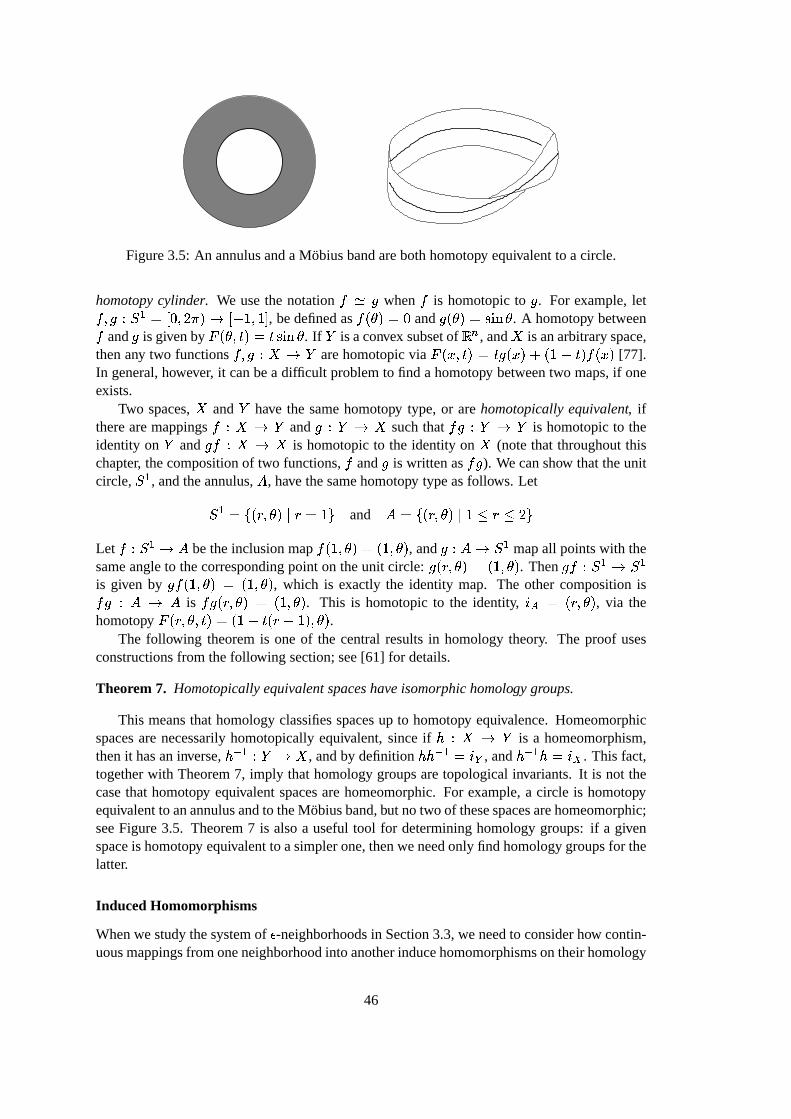
Figure3.5: An annulusandaMobiusbandarebothhomotopy equivalentto a circle.

homotopycylinder. We usethe notation ¤ z ¥when ¤ is homotopicto

¥. For example,let¤ ��¥ Y � ; � ,�% � D9² � #³,´HR+ � + - , bedefinedas ¤ ��µc�G� % and

¥<��µc�G�{¶:·` lµ. A homotopy between¤ and

¥is givenby © ��µb� � �d� � ¶:·` lµ

. If £ is aconvex subsetof A C , and�

is anarbitraryspace,thenany two functions ¤ ��¥ Y � #¸£ arehomotopicvia © ��­� � ��� � ¥¢��4� 5 � +¹H � � ¤ ��4�

[77].In general,however, it canbea difficult problemto find a homotopy betweentwo maps,if oneexists.

Two spaces,�

and £ have the samehomotopy type, or arehomotopicallyequivalent, iftherearemappings¤ Y � #¦£ and

¥ Y £º# �suchthat ¤ ¥ Y £»#¦£ is homotopicto the

identity on £ and¥ ¤ Y � # �

is homotopicto the identity on�

(notethat throughoutthischapter, thecompositionof two functions,¤ and

¥is written as ¤ ¥

). Wecanshow thattheunitcircle, � ;

, andtheannulus,¼ , have thesamehomotopy typeasfollows. Let� ; ��½��¾=�:µc���9¾¿� +�� and ¼ ��½��¾��:µb��� + �\¾$� Dg�Let ¤ Y � ; #À¼ betheinclusionmap ¤ � + �:µc�d�k� + �:µc�

, and¥ Y ¼W#¬� ;

mapall pointswith thesameangleto thecorrespondingpoint on theunit circle:

¥<��¾=�:µc�e�Á� + �:µc�. Then

¥ ¤ Y � ; #Â� ;is given by

¥ ¤ � + �:µc�®��� + �:µc�, which is exactly the identity map. The other compositionis¤ ¥ Y ¼Ã# ¼ is ¤ ¥<��¾=�:µc�®�Â� + �:µb�

. This is homotopicto the identity, Ä Å �Â��¾=�:µc�, via the

homotopy © ��¾=�:µb� � ���k� +�H � ��¾ H\+ �:�:µc�.

The following theoremis oneof the centralresultsin homologytheory. The proof usesconstructionsfrom thefollowing section;see[61] for details.

Theorem 7. Homotopicallyequivalentspaceshaveisomorphichomology groups.

This meansthathomologyclassifiesspacesup to homotopy equivalence.Homeomorphicspacesarenecessarilyhomotopicallyequivalent, sinceif / Y � # £ is a homeomorphism,thenit hasaninverse,/ [ ; Y £B# �

, andby definition /�/ [ ; � Ä Æ , and / [ ; / � Ä�Ç . This fact,togetherwith Theorem7, imply thathomologygroupsaretopologicalinvariants. It is not thecasethat homotopy equivalentspacesarehomeomorphic.For example,a circle is homotopyequivalentto anannulusandto theMobiusband,but notwo of thesespacesarehomeomorphic;seeFigure3.5. Theorem7 is alsoa usefultool for determininghomologygroups: if a givenspaceis homotopy equivalentto asimplerone,thenweneedonly find homologygroupsfor thelatter.

Induced Homomorphisms

Whenwe studythesystemof � -neighborhoodsin Section3.3,we needto considerhow contin-uousmappingsfrom oneneighborhoodinto anotherinducehomomorphismsontheirhomology

46

groups. A large amountof machineryhasbeendevelopedfor studyingthis type of problem.Wegiveabrief summaryhereandreferto Munkres[61] for moredetails.

SupposeÈ and É are two simplicial complexes andconsidera continuousmapof theirunderlyingspaces¤ Y � È@Ê � # � É �

. The first stepis to make a continuouspiecewise linearapproximationof ¤ , calledasimplicial approximation, / Y ÈË#ÃÉ . Thesimplicial complex Èis a subdivision of È@Ê , so

� È@Ê �b�Ì� È �. Thesubdivision is constructedto ensurethat / is close

to ¤ . “Close” meansthatgiven Q � È@Ê � , then ¤ ��4�

and / ��4�lie in thesamesimplex of É .

Thesimplicial approximation,/ , mapsverticesof È to verticesof É andextendslinearlyto eachsimplex of È . Sucha simplicial map, induceshomomorphismson the chaingroups/ÎÍ Y K 3 � È � # K 3 � É �

in a naturalway. If 2 3 � , �89� �>�>� �: 3 - is anoriented 1 -simplex of È ,thenwe define /�Í � 2 3 �d� ,�/ ��]8��:� �>�>� � / �� 3 ��- if ,�/ ���89�:� �>�>� � / �� 3 ��- Q É �/�Í � 2 3 �d� % otherwise�Thisdefinitionis extendedlinearly to all chains* 3 Q K 3 � È �

.Thecrucialpropertyof thechainmap /�Í is thatit commuteswith theboundaryoperator, i.e.,X � /ÎÍ � * 3 ����� /�Í � X � * 3 ��� . This impliesthat /ÎÍ mapscyclesin o 3 � È �

to cyclesin o 3 � É �andalso

boundariesto boundaries.This in turnmeansthat /�Í inducesahomomorphismof thehomologygroups, /ÎÏ Y r 3 � È � #¦r 3 � É �

. This homomorphismis definedon equivalenceclassesof 1 -cycles , w 3 - Q r 3 � È �

by: /ÎÏ � , w 3 -��Ð� ,�/�Í � w 3 ��- . See[35] for a proof that this definitionsatisfiesthepropertiesof ahomomorphism.

In the specialcasethat / Y � È � # � È �is the identity map,then /�Ï is the identity homo-

morphism. If / Y � È � # � É �is a homeomorphismof the underlyingspaces,then /�Ï is an

isomorphismof thecorrespondinghomologygroups.For acontinuousmap, ¤ , any simplicial approximationto ¤ inducesthesamegrouphomo-

morphism,denoted¤tÏ . The resultwe needfor Sections3.2.4and3.3 is thathomotopicmapsinduceidenticalhomomorphisms.

Theorem 8. Suppose¤ ��¥ Y � È � # � É �are two continuousmapsandthat ¤ is homotopicto

¥.

Thenthey inducethesamehomomorphismof thehomology groups,i.e., ¤ Ï �i¥ Ï .This is astandardresultin homology;see[61] for aproof.

3.2.3 Inversesystems

In orderto generalizehomologyto spaceswith infinite structurewe needto usea limit. Therearetwo waysto generalizethenotionof limit to generalindex setsandspaces:directandinverselimit systems.Ourprobleminvolvesthelatterandwedescribetheassociateddefinitionsbelow;seeHockingandYoung[35] or Spanier[77] for moredetails.

An inversesystemof topologicalspacesconsistsof collectionof spaces,��Ñ

, indexedby adirectedset

��ÒÓ�ÕÔ��, andcontinuousmappingsÖ Ñ>× Y � × # ��Ñ

, for eachpair Ø ÔTÙ. Themaps

arecalledbondingmorphismsandmustsatisfythefollowing two conditions.Ö ÑÕÑI� +�Ç�Ú �theidentitymapon

��ÑÎ�and (3.5)

Ö Ñ>× Ö ×=Û � Ö ÑÕÛg�for any choiceof Ü Ô Ø ÔfÙ � (3.6)

47

Notice that thesemapsactagainsttheorderrelation,which is why thesystemis an “inverse”one. We write Ý �Þ�L��Ñb� Ö Ñ>×]�:Ò��

for the inversesystem,or�L��ÑÎ� Ö Ñ>×Î�

whenthe index set isclearfrom context.

The inverselimit space, ß ·`àâá�ã Ý , is thesubspaceof äÓå ��Ñconsistingof all “preorbits” inÝ . Thatis, ß ·`àá�ã Ý ��½��]Ñc����]Ñ Q ��Ñ

andÖ Ñ>×]�� × �d�P]Ñfor Ø ÔiÙ ��� (3.7)

The projections, Ö × Y ß ·æà�á­ã ݸ# � ×, arethe continuousmapsÖ × ����]Ñc���I�Ì ×

. In fact, theinverselimit spaceis definedupto anisomorphism:any spacethatis homeomorphicto ß ·`àâá�ã Ýis alsoaninverselimit of Ý .

We canoftensimplify theinverselimit calculationby usinga subsetof theindex set,Ò Ê ?Ò

. The subsetmustbe cofinal for this restrictionto work, i.e., given anyÙ Q Ò

, thereis anelementØ Q Ò Ê with Ø ÔiÙ

. We thenhave thefollowing theorem[52].

Theorem 9. IfÒ Ê isacofinalsubsetof

Ò, thentheinversesystems

�L��Ñb� Ö Ñ>×]�:Ò��and

�L��Ñb� Ö Ñ>×]�:Ò Ê �haveisomorphiclimits — i.e., their inverselimit spacesare homeomorphic.

As anexampleof aninversesystem,supposetheindex setis thenon-negative integers, ç ,andlet

��8�� , % � + - , �è;Z� , % � ;� -�é , x� � + - and� 3 be the level-1 approximationto themiddle-

third Cantorset(c.f., Section2.2).Since� 3>n ; ? � 3 , for all 1 , thebondingmorphismsarejust

inclusionmaps: Ö 3�ê¿Y � êÓë # � 3 when ì � 1]�It is easyto show thatthesemapssatisfythetwo conditions(3.5)and(3.6). Theinversesystemis representedby thediagram:}>}>}Õí ��îbïH]# � 3 í �H]# � 3=[ ; }>}>} � x í=ðH�# �è; í ïH�# ��8 �Theinverselimit spaceconsistsof sequences

�� 3 � suchthat 3 Q � 3 for all 1 , andÖ 3�ê �� ê �u� 3 . Sincetheprojectionsareinclusionmaps,this means

3 �ñ ê . It follows thata sequencein the inverselimit spacejust repeatsthesamepoint, andthis point mustbe in theCantorset.Therefore,theinverselimit spaceis homeomorphicto themiddle-thirdCantorset.

Theconceptof inverselimit systemalsoexists for thecategory of groups.In this casethebondingmorphismsaregrouphomomorphismsandtheinverselimit is asubgroupof thedirectsum ò å y Ñ

of thegroupsin the inversesystem.We usethis in thenext sectionwhenwe de-fine Cechhomologyby relatinganinversesystemof topologicalspacesandthecorrespondinginversesystemof homologygroups.

3.2.4 Cechhomology

Cechhomologyis a generalhomologytheorythat cancapturethe infinitely detailedstructureof a fractal. It agreeswith simplicial homologyon finite simplicial complexes.For moreback-groundmaterial,seeHockingandYoung[35] or MardesicandSegal [52].

The nerve of a cover

TheCechapproachis basedon a way to generatesimplicial complexesby taking thenerveofa cover. Given a compactHausdorff space,

�, let ó �L���

denotethe family of all finite open

48

coveringsof�

(a covering, ô Q ó �L���, is a collection of opensetswhoseunion contains�

). We constructanabstractsimplicial complex, calledthenerve of thecover, by associatingeachopenset, õ Q ô with a vertex, alsolabelled õ , in thecomplex. An edgeexistsbetweentwo verticesõ and ö if andonly if thecorrespondingopensetsintersect.Higher-dimensionalsimplices ,�õ 8 �>�>��õ 3 - areincludedif theintersection÷ 3O`_ 8 õ O

is non-empty. Notethatalthoughthespace

�couldbelow dimensional,thenerve of agivencoveringcouldcontainmany high-

dimensionalsimplices.In fact,givenany finite simplicial complex È anda compact,perfect,Hausdorff space

�, it is possibleto constructa coveringof

�whosenerve is isomorphicto È

[35]. This ambiguityis removedby consideringaninverselimit system.

A partialorderrelation,Ô

, thatmakes ó �L���a directedsetis givenby thenotionof refine-

ment. Thecover ø is a refinementof ô , denotedø Ô ô , if for any set ö Q ø , thereis a setõ Q ô suchthat öù?Áõ . The family of all coverswith this orderingis the index setfor theCechinversesystem;we now definethebondingmorphisms.

If ø refinesô , wedefineaprojectionmapÖcú¢û Y ø~#¯ô by takingtheimageof aset ö Q ø ,Ö ú¢û � ö �, to beany fixedelementõ Q ô suchthat öÁ?fõ . Thedefinitionof theprojectionmap

is not uniquesincetheremay be more than one choiceof õ for a given ö . However, anytwo choicesof projectionfrom ø into ô are homotopic. Therefore,we definethe bondingmorphismsto be homotopy equivalenceclassesof projectionsÖ ú¢û , andthese“H-maps” thensatisfytheconditions(3.5) and(3.6). The inversesystem

� ô � Ö ú¢û � ó �L�����is referredto asthe

Cechsystem.Next, we considerthecorrespondinginversesystemof homologygroups.

The Cechhomologygroups

Thenerve of a finite cover ô is a simplicial complex, sowe cancomputeits homologygroupsby theusualtechniques.Thereis oneslight difference,however, thecoefficient group

ymust

bemoregeneralthantheintegers;for example,we couldusetherationalor realnumbers.Thehomologygroupsof the nerveswith coefficients in

yaredenotedr 3 � ô � y �

. The projectionmapsÖ ú¢û areidentifiedwith simplicial mapsof thenervesof ô and ø . They thereforeinducehomomorphismson thehomologygroups:Ö ú4û Ï Y r 3 � ø � y � #¬r 3 � ô � y �

. Theorem8 impliesthat two elementsof the homotopy classof Ö ú¢û inducethe samehomomorphismon the ho-mologygroups.Theinversesystem

� r 3 � ô � y �:� Öjú¢û Ï � ó �L�v���is calledthe 1 th Cechhomology

system.Finally, the 1 th Cechhomologygroupwith coefficientsiny

is denoted ür 3 �L��� y �and

is definedto betheinverselimit of the 1 th Cechhomologysystem.

Geometrically, supposethereis a non-bounding1 -cycle w 3 in r 3 � ô � y �for some ô Qó �L�v�

. Thenthis 1 -cycleexistsin thelimit only if givenany refinementø of ô , thereisa 1 -cyclew Ê3 Q r 3 � ø � y �whoseimageundertheprojectionhomomorphismis w 3 , i.e., Ö ú4û Ï � w Ê3 �d� w 3 .

The Cechsystemfor all finite coversof the space�

is overwhelminglylarge for compu-tationalpurposes;this is why cofinal subsetsareuseful. A subcollection,ó Ê �L��� ?Áó �L���

, iscofinal in ó �L���

if given any cover ô Q ó �L�v�, thereis a cover ø Q óýÊ �L���

suchthat ø is arefinementof ô . As anexample,if we have a compactspace

� ?PA�þ , let ô C bea finite coverof

�by openballs with diameter+ s 0 . Thecollectionof all suchcoveringsfor 0 Q~S

formsa cofinal subsetof ó �L���

. We cannow setup a Cechsystemfor this subfamily of coveringsandcomputethecorrespondinginversesystemof homologygroups.By Theorem9, theinverselimit of this systemis isomorphicto the inverselimit of the full Cechsystem.Thus,usingacofinal family of coveringsgreatlyreducestheamountof work neededto “compute” theCechhomologygroups.Theuseof cofinalfamiliesis alsoimportantin ourcomputationalwork.

49

A

B

C

A B

C

Figure3.6: Thelevel-1 cover of theSierpinskitriangleandthenerve of this cover. Thehigherlevel coversrepeatedthispatternon smallerscales.

Figure3.7: Nervesof the level-3, level-2, and level-1 coversof the Sierpinskitriangle. Thearrows show theactionof theprojectionmapson thecircledtriplesof points.

An example

Weuseacofinalsequenceof coversof theSierpinskitriangle,ÿ , to computeits Cechhomologygroups.This exampleis consideredfurtherin Section3.5.

For Ä � % � + � D � E � �>�>� , let ô Obe a cofinal sequenceof covers of ÿ with the following

properties. The setsin eachcover are identical openconvex regions with different centers.Thereare E O suchopensetsin ô O

such that for each õ O�Q ô Othereare exactly threesetsõ O n ;�� ö O n ;=��� O n ; Q ô O n ;

that mapinto õ O, andeachpoint of the Sierpinskitrianglebelongs

to at mosttwo of thesetsin ô O. SeeFigure3.6 for an illustrationof the level-1 cover, ô ;

andits nerve. Thelastconditionimpliesthat thenerve of ô O

hasonly 0-simplicesand1-simplices.Thenervesfor ô ;

, ô x , and ô � aregiven in Figure3.7. This figurealsoshows theactionof thebondingmorphisms,Ö O�� O n ; Y ô O n ; #Âô O

, which aredefinedby the inclusionof the threesetsõ O n ;�� ö O n ;=��� O n ; Q ô O n ;into õ OGQ ô O

.The simple,one-dimensionalnatureof the nervesmeansthat we canwrite down the ho-

mology groupsby inspection. The zerothandsecondhomologygroupsare the samefor all

50

a b

c

d

d

p12

1

2

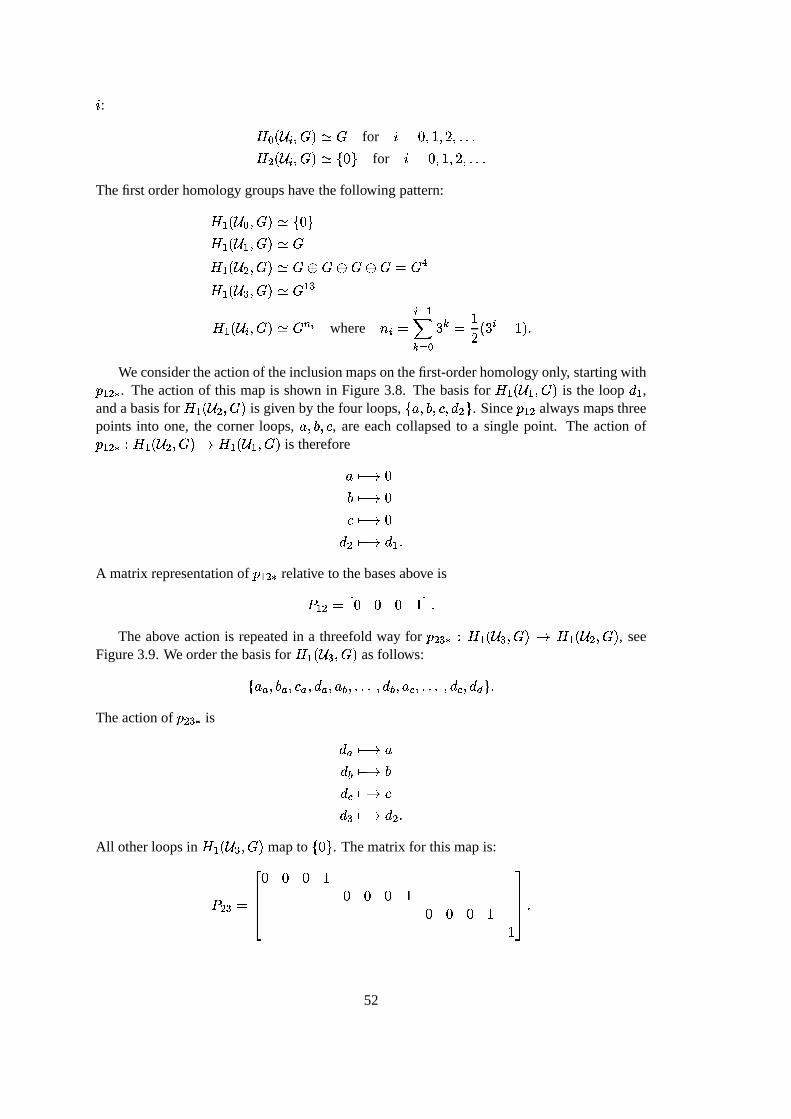
Figure3.8: Theprojectionmapfrom ô x into ô ;.

a b

c

d

d

d

da b

c

a a

a

b b

b

c c

p23

d23

a a

a

b b

b

c c

cc

Figure3.9: Theprojectionmapfrom ô � into ô x .

51

Ä : r 89� ô O � y � zWyfor Ä � % � + � D � �>�>�r x � ô O � y � z � %j� for Ä � % � + � D � �>�>�

Thefirst orderhomologygroupshave thefollowing pattern:r ; � ô 8 � y � z � %j�r ;�� ô ;=� y � z{yr ; � ô x � y � z{y | y | y | y � y��r ;�� ô � � y � z{y ; �r ;=� ô O � y � z{y C�� where 0 O � O [ ;^3 _ 8 E 3 � +D � E O H\+ � �Weconsidertheactionof theinclusionmapsonthefirst-orderhomologyonly, startingwithÖ ; x Ï . Theactionof this mapis shown in Figure3.8. The basisfor r ; � ô ; � y �

is the loop� ;

,andabasisfor r ;�� ô x � y �

is givenby thefour loops,� ' �)(=� * �:� x � . SinceÖ ; x alwaysmapsthree

points into one, the cornerloops, ' �)(=� * , areeachcollapsedto a singlepoint. The actionofÖ ; x Ï Y r ;�� ô x � y � #Àr ;�� ô ;=� y �is therefore'� H]#À%( � H]#À%*� H]#À%� x � H]# � ; �

A matrix representationof Ö ; x Ï relative to thebasesabove is� ; x � � % % % +��d�The above actionis repeatedin a threefoldway for Ö x � Ï Y r ;=� ô � � y � # r ;�� ô x � y �

, seeFigure3.9. Weorderthebasisfor r ;=� ô � � y �

asfollows:� '�� �)( � � *�� �:� � � '�� � �>�>� �:� � � '�� � �>�>� �:� � �:� þ ���Theactionof Ö x � Ï is � � � H]#À'� ��� H]# (� � � H]#À*� � � H]# � x �All otherloopsin r ;�� ô � � y �

mapto� %j� . Thematrix for thismapis:

� x � � ���� % % % + % % % + % % % + +����� �

52

1-n

1-2

, )(

1-n

( ,1)

. . .

(0,0) (1,0)

(0,1) (1,1)

Figure3.10: The Warsaw circle hastrivial simplicial homologygroup, r ; � % , but its Cechhomologygroupis ür ;ý� y

. It hasthesame“shape”asthecirclebecausethey arebothinverselimits of asequenceof annuli.

This patterncontinuesfor higher levels, andfor Ö O�� O n ; Ï Y r ;�� ô O n ;=� y � # r ;�� ô O � y �we

have therecursive form for thematrix

� O�� O n ; � ���� � O [ ; � O � O [ ; � O � O [ ; � O +����� �

This meansthat the first Cechhomologygroup for the Sierpinski triangle, ür ;=� ÿ � y �is

an infinitely generatedabeliangroup. The elementsof ür ; � ÿ � y �consistof sequences,

� w O � ,of elements,w O\Q r ;=� ô O � y �

, such that Ö O�� O n ; Ï � w O n ;��\� w O for all Ä � + � D � E � �>�>� . Forexample, the central hole in the Sierpinski triangle would be representedby the sequence��� O ���¬���c;=�:� x �:� � � �>�>� � , and the ' -loop of ô x by

� ' O ���¬� % � ' �:� � � �>�>� � . Smallerholeshavea longerinitial stringof zeros.

The next sectiongeneralizesCechhomologyby consideringinverselimit systemsof ap-proximatingspacesotherthannervesof covers.

3.2.5 Shapetheory

Shapetheorygeneralizestheconceptof homotopy equivalenceby consideringinversesystemsof “nice” approximatingspaces. As an example, the unit circle hasthe sameshapeas theWarsaw circle of Figure3.10,becausebothareinverselimits of sequencesof annuli,althoughthey have differenthomotopy andsimplicial homologygroups.

Theessentialresultwe usefrom shapetheoryis thatevery compactmetricspaceis home-omorphicto the limit of an inversesystemin the category of finite polyhedraandhomotopyequivalenceclassesof maps(H-maps). The Cechsystemfor a compactspaceis an exampleof suchan inversesystem. Shapetheorygeneralizesthe Cechapproachby allowing the ap-proximatingspacesto behomotopy equivalentto afinite polyhedron.Thefollowing theoremisa compilationof resultsfrom MardesicandSegal [52, App.1]; it characterizesspacesthatarehomotopy equivalentto finite polyhedra.

Theorem 10. A topological spacewith thehomotopytypeof a compactCW-complex or a com-pactANRis homotopyequivalentto a compactpolyhedron.

53

CW-complexesaregeneralcell-complexes,andANR standsfor absoluteneighborhoodre-tract; see[35] for definitions. ANRs arean importantclassof space;they have many usefulproperties— oneof theseis that theidentity mapextendsto a neighborhoodof thespace(thisis theneighborhoodretractpartof ANR). Theunit cubein AGC andthe 0 -sphereareexamplesof ANRs.

Thealgebraicsideof shapetheoryassociatesan inversesystemof homologygroupswiththeinversesystemof finite polyhedra,in muchthesamemannerasCechhomology. Thatis, if���dÑb� Ö Ñ>×��

is aninversesystemof polyhedra,then� r 3 ���dÑc�:� Ö Ñ>× Ï � is thecorrespondinginverse

systemof homologygroups.A third resultwe needfrom shapetheoryis:

Theorem 11. If���dÑb� Ö Ñ>×��

and���¿ÑÎ���ÕÑ>×Î�

are inversesystemsof polyhedra (or ANRsor CW-complexes)and H-mapswhoseinverse limit spacesare homotopyequivalent,thenthe corre-spondinginversesystemsof homology groupshaveisomorphiclimits.

For a compactspace,�

, the Cechsystemis an inversesystemof polyhedra. The abovetheoremthereforeimplies thatany otherinversesystemof polyhedrayieldsan inversesystemof homologygroupswhoselimit isomorphicto Cechhomology. This is the sensein whichshapetheorygeneralizesCechhomology.

In the following sectionwe consideran inversesystemof closed� -neighborhoodsandin-clusionmapsfor acompactspace

�.

3.3 Foundationsfor computing homology

In this sectionwe develop theoreticalfoundationsfor understandinghow homologygroupscomputedfrom datarelateto thehomologyof thespacethey approximate.Thesettingfor ouranalysisis asfollows. Weassumethattheunderlyingspace,

�, is acompactsubsetof ametric

space,���W�:��

, andthatthefinite setof points, �f? �, approximates

�in a metricsense,i.e.,

eachpoint of�

is within distance� of somepoint in � andvice versa.In otherwords, � is theHausdorff distancebetween

�and � :

�� �L�¨� � �l� � . In a givenapplication,this assumptionmustbejustifiedby physicalor numericalarguments;we give a numberof differentexamplesin Chapter4. A smallvalueof � implies � is agoodapproximationto

�. Typically, � depends

on thenumberof pointsin � , aswedemonstratedwith examplesin Chapter2, andmorepointsnaturallyresultin a smallervalueof � . In someapplications,� couldrepresentthemagnitudeof noisepresentin thedata,or adiscretizationerror.

To give the compactspace,�

, and its finite approximation, � , comparabletopologicalstructure,we form their closed� -neighborhoods:���G� �� Q � �9������������ ��� and � �G��� Q � ���]��­� � ��� �����Roughly speaking,since

�and � are within � , their � -neighborhoodsshouldhave similar

propertiesfor � � � . Wemake thisprecisein Section3.3.4usinganinversesystemframeworkfrom shapetheory. Sincethe homologyof

���convergesto the homologyof

�as �â# % in

an inverselimit sense,we hopeto extrapolatethe homologyof�

from the homologyof the� -neighborhoodsof thedata, � , for � � � . Of course,extrapolationis never guaranteedto givethecorrectanswer, andwe arealwaysrestrictedby theinherentaccuracy of thefinite data.

3.3.1 The inversesystemof ! -neighborhoods

We begin by describingthe inversesystemof � -neighborhoodsfor theunderlyingcompactset�. Thespacesfor theinversesystemaretheclosed� -neighborhoods,

���G� ��@�9�]��­������� ��� ,

54

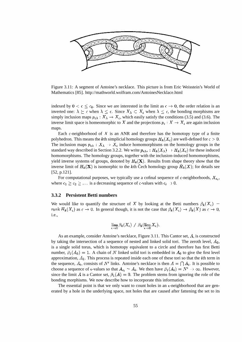
Figure3.11: A segmentof Antoine’s necklace.This pictureis from Eric Weisstein’s World ofMathematics[85]. http://mathworld.wolfram.com/AntoinesNecklace.html

indexedby %#"k� � � 8 . Sincewe areinterestedin the limit as ��#°% , theorderrelationis aninvertedone:

ÙTÔ � whenÙi� � . Since

��Ñ ? ���when

Ùf� � , thebondingmorphismsaresimply inclusionmapsÖ � Ñ Y ��Ñ # ���

, whicheasilysatisfytheconditions(3.5)and(3.6). Theinverselimit spaceis homeomorphicto

�andtheprojectionsÖ � Y � # ���

areagaininclusionmaps.

Each � -neighborhoodof�

is an ANR and thereforehasthe homotopy type of a finitepolyhedron.Thismeansthe 1 th simplicialhomologygroupsr 3 �L���:�

arewell-definedfor � � % .The inclusionmapsÖ � Ñ Y ��Ñ # ���

inducehomomorphismson the homologygroupsin thestandardwaydescribedin Section3.2.2.Wewrite Ö � Ñ Ï Y r 3 �L��Ñc� #Ãr 3 �L���)�

for theseinducedhomomorphisms.Thehomologygroups,togetherwith theinclusion-inducedhomomorphisms,yield inversesystemsof groups,denotedby r 3 � Ý �

. Resultsfrom shapetheoryshow that theinverselimit of r 3 � Ý �

is isomorphicto the 1 th Cechhomologygroup ür 3 �L���; for detailssee

[52, p.121].For computationalpurposes,we typically usea cofinalsequenceof � -neighborhoods,

��� � ,where � ; Ui� x Uh�>�>� is adecreasingsequenceof � -valueswith � O #À% .

3.3.2 PersistentBetti numbers

We would like to quantify the structureof�

by looking at the Betti numbers� 3 �L��� �±��)�t b¡ r 3 �L���:�as �Ó#°% . In generalthough,it is not thecasethat � 3 �L���:� #�� 3 �L���

as �Ó#�% ,i.e., ß ·`à��$¿8 � 3 �L���:�&%� � 3 � ß ·æà��$¿8 ���)� �

As anexample,considerAntoine’snecklace,Figure3.11.ThisCantorset, ¼ , is constructedby taking the intersectionof a sequenceof nestedandlinked solid tori. Thezerothlevel, ¼ 8

,is a singlesolid torus,which is homotopy equivalent to a circle and thereforehasfirst Bettinumber, � ;�� ¼ 8���� + . A chainof ' linked solid tori is embeddedin ¼ 8

to give thefirst levelapproximation,¼ ;

. This processis repeatedinsideeachoneof thesetori sothatthe Ä th terminthesequence,¼ O

, consistsof ' Olinks. Antoine’s necklaceis then ¼ � ÷~¼ O

. It is possibletochoosea sequenceof � -valuessothat ¼ � � z ¼ O

. We thenhave � ; � ¼ O �u� ' O #)( . However,sincethelimit ¼ is a Cantorset, � ;�� ¼ �ý� % . Theproblemstemsfrom ignoringtherole of thebondingmorphisms.Wenow describehow to incorporatethis information.

Theessentialpoint is thatwe only want to countholesin an � -neighborhoodthataregen-eratedby a hole in theunderlyingspace,not holesthatarecausedafter fatteningthesetto its

55

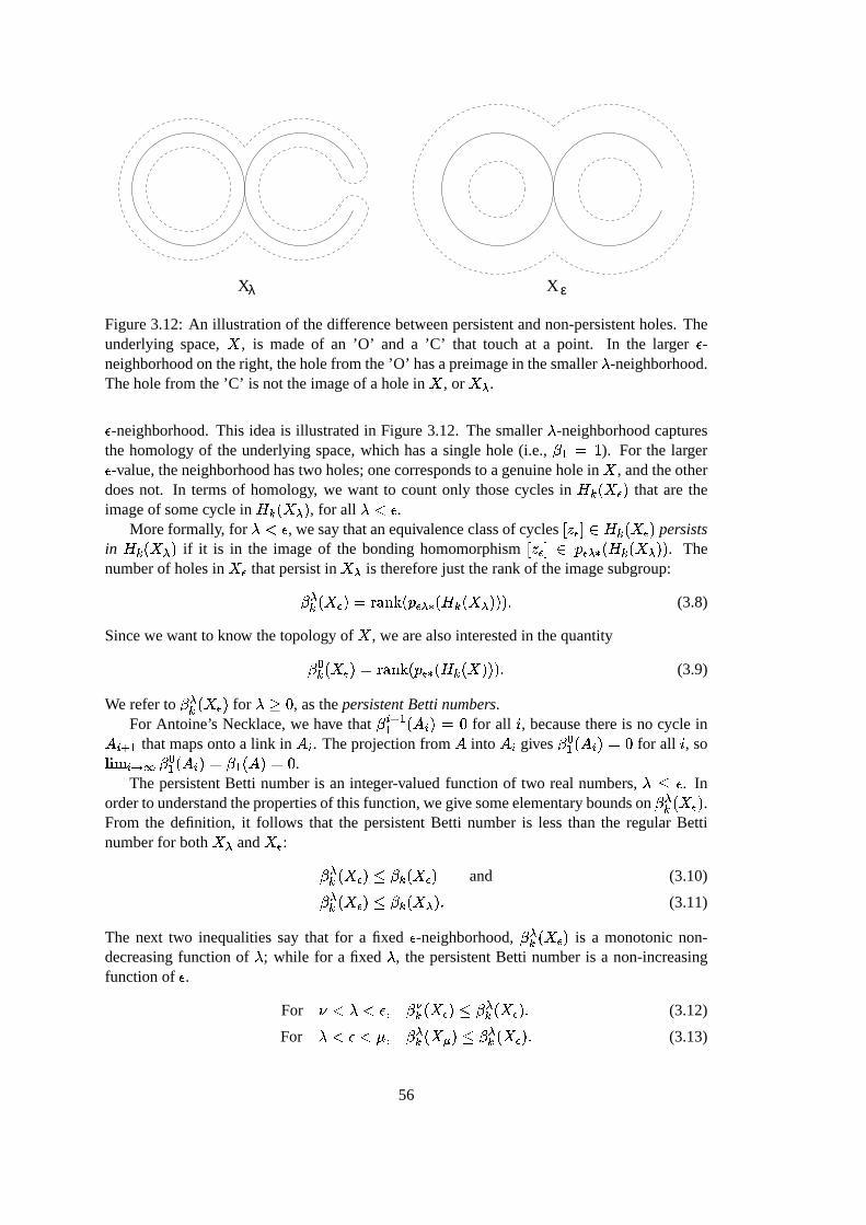
εXλ X

Figure3.12: An illustrationof thedifferencebetweenpersistentandnon-persistentholes.Theunderlyingspace,

�, is madeof an ’O’ and a ’C’ that touch at a point. In the larger � -

neighborhoodontheright, theholefrom the’O’ hasapreimagein thesmallerÙ-neighborhood.

Theholefrom the’C’ is not theimageof aholein�

, or��Ñ

.� -neighborhood.This ideais illustratedin Figure3.12. ThesmallerÙ-neighborhoodcaptures

the homologyof the underlyingspace,which hasa singlehole (i.e., � ; � + ). For the larger� -value,theneighborhoodhastwo holes;onecorrespondsto agenuineholein�

, andtheotherdoesnot. In termsof homology, we want to countonly thosecycles in r 3 �L���)�

that are theimageof somecycle in r 3 �L��Ñc�

, for allÙ "i� .

More formally, for٠"i� , wesaythatanequivalenceclassof cycles , w � - Q r 3 �L���)�

persistsin r 3 �L��Ñb�

if it is in the imageof the bondinghomomorphism, w � - Q Ö � Ñ Ï � r 3 �L��Ñc���. The

numberof holesin���

thatpersistin��Ñ

is thereforejust therankof theimagesubgroup:� Ñ3 �L��� �d�T�)�t b¡¢� Ö � Ñ Ï � r 3 �L��Ñc����� � (3.8)

Sincewewantto know thetopologyof�

, we arealsointerestedin thequantity� 83 �L��� �d�T� �t b¡<� Ö � Ï � r 3 �L������� � (3.9)

Wereferto � Ñ3 �L���)�for

Ù U\% , asthepersistentBetti numbers.For Antoine’s Necklace,we have that � O n ;; � ¼ O ��� % for all Ä , becausethereis no cycle in¼ O n ;

thatmapsontoa link in ¼ O. Theprojectionfrom ¼ into ¼ O

gives � 8; � ¼ O �G� % for all Ä , soß ·`à O $+* � 8; � ¼ O ��� � ; � ¼ ��� % .The persistentBetti numberis an integer-valuedfunctionof two realnumbers,

Ùf� � . Inorderto understandthepropertiesof this function,wegivesomeelementaryboundson � Ñ3 �L���:�

.From the definition, it follows that the persistentBetti numberis lessthan the regular Bettinumberfor both

��Ñand

���: � Ñ3 �L���:�Ð� � 3 �L���)�

and (3.10)� Ñ3 �L���:�Ð� � 3 �L��Ñb� � (3.11)

The next two inequalitiessay that for a fixed � -neighborhood,� Ñ3 �L� � �is a monotonicnon-

decreasingfunction ofÙ; while for a fixed

Ù, the persistentBetti numberis a non-increasing

functionof � .For Ü," Ù "i� � � Û3 �L���:�u� � Ñ3 �L���)� � (3.12)

ForÙ "i�"\Ø � � Ñ3 �L� × �Ð� � Ñ3 �L���)� � (3.13)

56

Roughlyspeaking,increasingthedifferencebetweenÙ

and � decreasesthenumberof persistentholes.

The above inequalitiesarea first steptowardsunderstandingthe continuity propertiesof� Ñ3 �L���)�, but morework remainsto bedone.Most importantly, we wantconditionson

�that

guarantee � 83 �L���)� #N� 3 �L���as �ý#À%c� (3.14)

If � 3 �L�v�is finite and(3.14)holds,thentheremustbean � 8 � % suchthat � 83 �L��� �d� � 3 �L���

for� Q , % � � 8�� . In additionto this,our computationalwork will bemosteffective for spaceswherethereis a

Ù 8suchthat � Ñ3 �L� � �¹� � 83 �L� � �

forÙ Q , % �)Ù 8 -

. We do not expecttheseconditionsto hold for anarbitrarycompactspace.However, for specialcasessuchastheiteratedfunctionsystemattractorsin Section3.5, it maybepossibleto saysomethingmoreconcreteaboutthecontinuityof persistentBetti numbersas

Ùand � tendto zero.

3.3.3 Growth rates for persistentBetti numbers

In Chapter2, we quantifiedthe rateof growth in thenumberof connectedcomponents,K � � �

by the disconnectednessindex, - . We cando the samething for the 1 -dimensionalholes,ascountedby the persistentBetti numbers.If � 83 �L��� � # ( as �â# % , we quantify the rateofdivergenceby assumingan asymptoticpower law, � 83 �L� � �/. �10 � . The exponent - 3 canbecomputedasthefollowing limit (whenit exists)

- 3 � ß ·`à��$¿8 ß3254u� 83 �L��� �ß3254 � + s � �f� (3.15)

If thelimit doesnotexist, thenwe usethelimsupor liminf.Recallthatfor 1 � % , theBetti numberis just thenumberof connectedcomponents,sothe

definition of - 8 agreeswith that for the disconnectednessindex, - . The + -dimensionalholescountedby � 8;

arereally loops,andthe 2-dimensionalholesaresphericalvoids like thoseinSwisscheese,sowemightcall - ; theloopinessindex and - x theholiness.Resultsin Chapter5show that for subsetsof A x , thereis a relationshipbetween- ; andthe fractal dimension;theexamplesin Section3.5confirmthis.

SimpleExamples

We candeterminethegrowth rates,- 3 , analyticallyfor simple,self-similarfractalsuchastheSierpinskitriangle,Sierpinskicurve (or carpet),Mengerspongeandso on. We alreadycon-sideredthe homologygroupsfor the Sierpinskitriangle, ÿ , in Section3.2.4. It is possibletochoosea sequenceof � -valuesso that thehomologygroups r ;=� ÿ � � �¹� r ;=� ô O �

. Specifically,let

¾be the radiusof the largestcircle inscribedby the triangularholewith verticesat

� ;x � % �,� % � ;x �

and� ;x � ;x �

, sothat¾R� ;x H76 x�98 %c�`+�:�;�:�< . Sincethenext largestholehasradius

¾ s D , wechoose

¾ s D#"{� ; " ¾and � O n ;¿� � O s D . Every element,, w ;)- Q r ;=� ÿ � � � , hasa preimageunder

theprojectionmap,Ö � � Ï Y ür ; � ÿ � # r ; � ÿ � � � , sothepersistentBetti numberis thesameastheregularBetti number. Fromourpreviouscalculations,then, � 8; � ÿ � � ��� 0 O �k� E O H\+ � s D . Thus,

- ; � ß ·`à�=$R8 ß>254 � � 8; � ÿ � � ���ß3254 � + s � O � � ß ·`àO $+* ß3254 ��� E O Hi+ � s D �ß3254�D O s � ; � ß>254ÐEß>254ÐD � (3.16)

Not surprisingly, thisnumberis thesameasthesimilarity dimension.

57

3.3.4 Finite approximations

We now analyzethefinite approximation,� , andits relationshipto thecompactset�

. As de-scribedin theintroductionto this section,we assumethattheHausdorff distance,

� �L�¨� � �u�� , i.e., that� ?q�@? and �h? � ? . We keepthenotation,

�L���)� Ö Ñ � �, for the inversesystemsof� -neighborhoodsof

�andwrite

� � �)���ÕÑ � �for thesystemof neighborhoodsof � . Theinclusions

of � into� ? and

�into �@? givea formal relationshipbetweentheseinversesystemsandallow

usto deriveboundsonthepersistentBetti numbersof���

in termsof � -persistentBetti numbersof � �

.Since

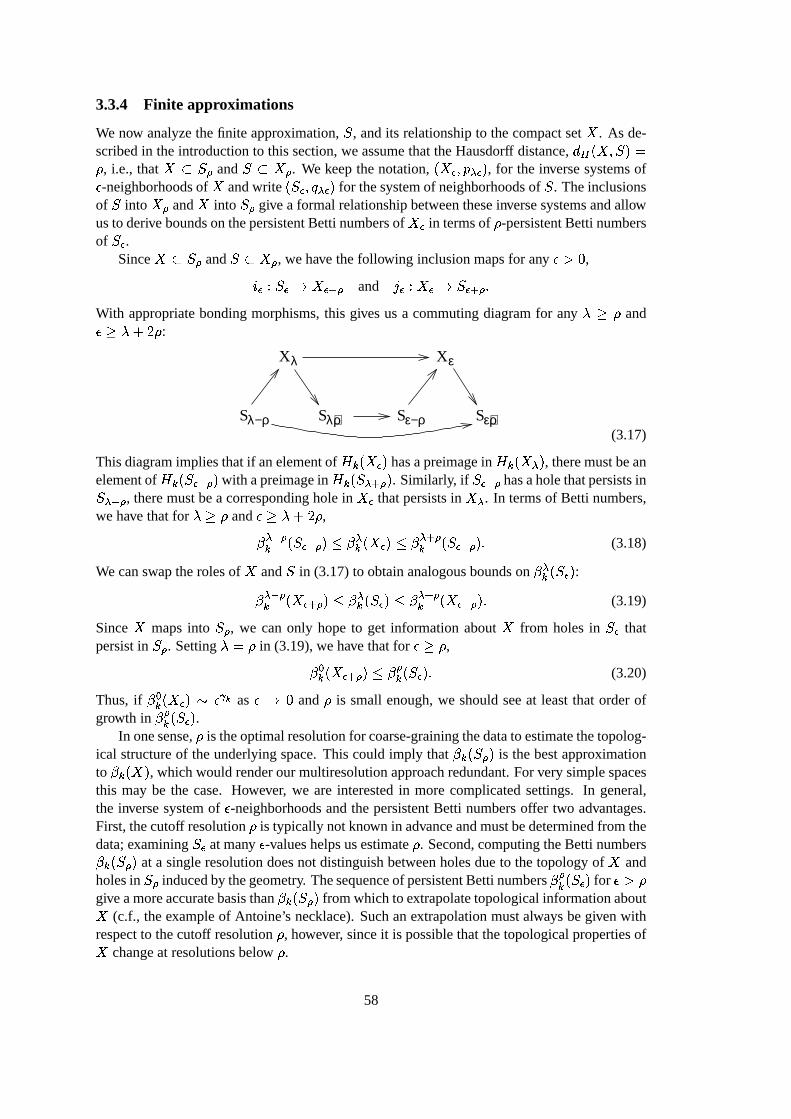
� ?f�@? and �\? � ? , wehave thefollowing inclusionmapsfor any � � % ,Ä � Y � � # ��� n ? and ì � Y ��� #¬� � n ?t�With appropriatebondingmorphisms,this givesus a commutingdiagramfor any

٠UB� and��U ٠5~D�� :

Xλ Xε

ε+ρε−ρλ+ρλ−ρS S S S(3.17)

Thisdiagramimpliesthatif anelementof r 3 �L���)�hasapreimagein r 3 �L��Ñc�

, theremustbeanelementof r 3 � � � [ ? � with apreimagein r 3 � � Ñ n ? � . Similarly, if � � n ? hasaholethatpersistsin� Ñ [ ? , theremustbea correspondingholein

� �thatpersistsin

��Ñ. In termsof Betti numbers,

we have thatforÙ U~� and �6U Ù 5\D�� ,� Ñ [ ?3 � � � n ? �u� � Ñ3 �L���:�ý� � Ñ n ?3 � � � [ ? � � (3.18)

Wecanswaptherolesof�

and � in (3.17)to obtainanalogousboundson � Ñ3 � � �)�:� Ñ [ ?3 �L��� n ? �Ð� � Ñ3 � � ���ý� � Ñ n ?3 �L��� [ ? � � (3.19)

Since�

mapsinto �A? , we canonly hopeto get informationabout�

from holesin � �that

persistin �@? . SettingÙV� � in (3.19),we have thatfor �6U~� ,� 83 �L��� n ? �Ð� � ?3 � � �)� � (3.20)

Thus, if � 83 �L��� �B. �C0 � as �â# % and � is small enough,we shouldseeat leastthat orderofgrowth in � ?3 � � �:�

.In onesense,� is theoptimalresolutionfor coarse-grainingthedatato estimatethetopolog-

ical structureof theunderlyingspace.This could imply that � 3 � � ? � is thebestapproximationto � 3 �L�v�

, whichwould renderourmultiresolutionapproachredundant.For verysimplespacesthis may be the case. However, we are interestedin morecomplicatedsettings. In general,the inversesystemof � -neighborhoodsandthepersistentBetti numbersoffer two advantages.First,thecutoff resolution� is typically notknown in advanceandmustbedeterminedfrom thedata;examining � �

atmany � -valueshelpsusestimate� . Second,computingtheBetti numbers� 3 � �@? � at a singleresolutiondoesnot distinguishbetweenholesdueto thetopologyof�

andholesin � ? inducedby thegeometry. Thesequenceof persistentBetti numbers� ?3 � � � �

for � � �giveamoreaccuratebasisthan � 3 � �@? � from whichto extrapolatetopologicalinformationabout�

(c.f., theexampleof Antoine’s necklace).Suchanextrapolationmustalwaysbegivenwithrespectto thecutoff resolution� , however, sinceit is possiblethatthetopologicalpropertiesof�

changeat resolutionsbelow � .

58

3.3.5 Computing persistentBetti numbers

Wewanttocomputethenumberof holesin � �thatpersistin �@? , thatis, � ?3 � � �:���f� �t b¡D��� ?"Ï � r 3 � �@? ��� .

This definition is in termsof the rank of a linear operator,�Õ� ? Ï , on the two quotientspaces,r 3 � �@? � and r 3 � � �)�

. Below, wederiveanequivalentformulathatis givenin termsof thelinearmapon thechaingroups,

� � ? Í Y K 3 � �@? � # K 3 � � �)�. Recallthatthe 1 -simplicesform abasisfor

the 1 th chaingroup,soit is easyto write down amatrix representationfor thismap.To simplify notationa little, we write:K ? for thechaingroup

K 3 � �A? �:�K �for

K 3 � � �)�:�� Í for thechainmap� � ? Í �� Ï for thehomologyhomomorphism

�Õ� ? Ï �oE? � o �for thecyclegroupsp�? � p �for theboundarygroups,andr ? � o ? s p ? andr ��� o � s p �for thehomologygroups.

Our startingpoint is the imagegroup,� Ï � rF? � ? r �

. Oneof thefundamentaltheoremsabouthomomorphismsof groups[34] is that theimageof a group,

y, undera homomorphism,G , is

isomorphicto thequotient,y s ¡5H>� G . Thus,� Ï � rF? � z r? s ¡5H>�@� Ï=�

Thekernel,¡5H>�I� Ï , containsall elementsof rF? thatmapto thezeroelementof r �

. Thatis,¡5H>�J� Ï � � , w - Q r? � , � Í � w ��-­� , % - Q r � ���But acycle is homologousto % if andonly if it is in theboundarygroup,so¡5H>�J� Ï z o ?DK � [ ;Í � p � � �

Now, recall from Section3.2.2 that a homomorphisminducedby a simplicial mapcom-muteswith the boundaryoperator. It follows that cycles map to cycles and boundariestoboundaries;i.e., � Í � oL? � ?fo �

and� Í � p�? � ?\p � �

Thesecondexpressionimpliesthat p�? ? � [ ;Í � p �)�, so p�?Z?hoL? K � [ ;Í � p �:�

. It follows thatthequotient � Ï � r? � z r? s ¡5H>�J� Ï z ,�oL? s p�? - s ,�oL? K � [ ;Í � p �)��- z oE? s ,�oL? K � [ ;Í � p �)��- �Finally, thismeansthatthepersistentBetti numberis� ?3 � � �d�T�)�t Î¡ ,�o ? - H �)�t b¡ ,�o ?DK � [ ;Í � p � ��- � (3.21)

In termsof actualcomputation,then, we can find the persistentBetti numberfrom thedimensionsof null spacesandrangesof matrix representationsfor theboundaryoperatorandtheinclusionmaps.Specifically,

�)�t b¡ o 3 � � �is thedimensionof thenull spaceof thematrix for

59

X 3 � � � Y K 3 � � � # K 3=[ ; � � �. For thesecondtermin (3.21)weneedto find theintersectionof two

spaces:� Í:,  �M ß`ß � X 3 � � ����-

, and p �, which is the rangeof X 3>n ; � � � Y K 3>n ; � � � # K 3 � � � . Finding

the intersectionof two linear subspacesrequiressomeinformation abouttheir bases,and isthereforea moredifficult problemthancomputingdimensions.The standardalgorithmsfordeterminingintersectionstypically run in N � 04� � time, where 0 is the largestdimensionof thematricesinvolved [29]. As we discussin the following section,we have not yet implementedthesealgorithms. Instead,for the examplesof Section3.5 we usepre-existing software forcomputingtheregularBetti numbersfrom subsetsof a triangulationdescribedin Section3.4.1.Theseexamplesillustratewhy theregularBetti numbersareinsufficient for extrapolation.

3.4 Implementation

Our goal is to take a finite cloudof points � asinput,andcomputepersistentBetti numbersasa functionof a resolutionparameter. Therearefour partsto theoverall process:

1. Forasequenceof � -values,generatesimplicialcomplexesthattriangulatethe � -neighborhoodsof thedata.

2. Estimatethecutoff resolution� .

3. ComputepersistentBetti numbers,� ?3 � � � , for � � � .

4. If appropriate,computethegrowth rate, - 3 .

This is essentiallythesameapproachwe usedin Chapter2 in computingthe numberof con-nectedcomponents.For that case,however, a simplicial complex is unnecessary— all theinformationabout � -connectedcomponentsof � is encodedin theEuclideanminimal spanningtreeof thedata.

In thepresentcontext, steps1 and3 arethemostcomputationallyintensive. Thetwo stepsarealsocloselyrelated;efficient algorithmsfor computingBetti numbersmake explicit useofthedatastructuresinvolved in building thecomplexes.Thus,givenan � -neighborhood,� �

, thefirst problemis to generatea simplicial complex, F �

, whoseunderlyingspaceis at leasthomo-topy equivalent to � �

. Sincewe are interestedin the inversesystemof � -neighborhoods,weneedsimplicial complexesfor a sequenceof numbers� O #¸% . In orderto have inclusionmapsthatarewell defined,weneedF � � to beeitherasubcomplex or asubdivisionof F �PO

when � O "i� ê .A subcomplex approachto this problemdueto Edelsbrunneret al. [18], is describedin detailin Section3.4.1. This grouphasalsodevelopeda fast incrementalalgorithmfor computingBetti numbersof complexes in A x or Ae� . We usetheir implementationsfor the examplesinSection3.5.

We usethe samecriterion for Step2 that we derived in Chapter2 for approximationstoperfectspaces.Sincea perfectspacehasno isolatedpoints,we estimatethecutoff resolutionas the largestvalue of � for which � �

hasat leastone isolatedpoint. This underestimatesthevaluefor which �@?/Q �

, but theexamplesin Section3.5 show it to bea reasonablygoodapproximation.Recallthatisolatedpointsarestraightforwardto detectnumerically— apointis� -isolatedif thedistancefrom it to everyotherpoint in thesetis greaterthan � . Thecomputationof growth ratesin Step4 is straightforwardoncethepersistentBetti numbersarefound.

60

(a) (b)

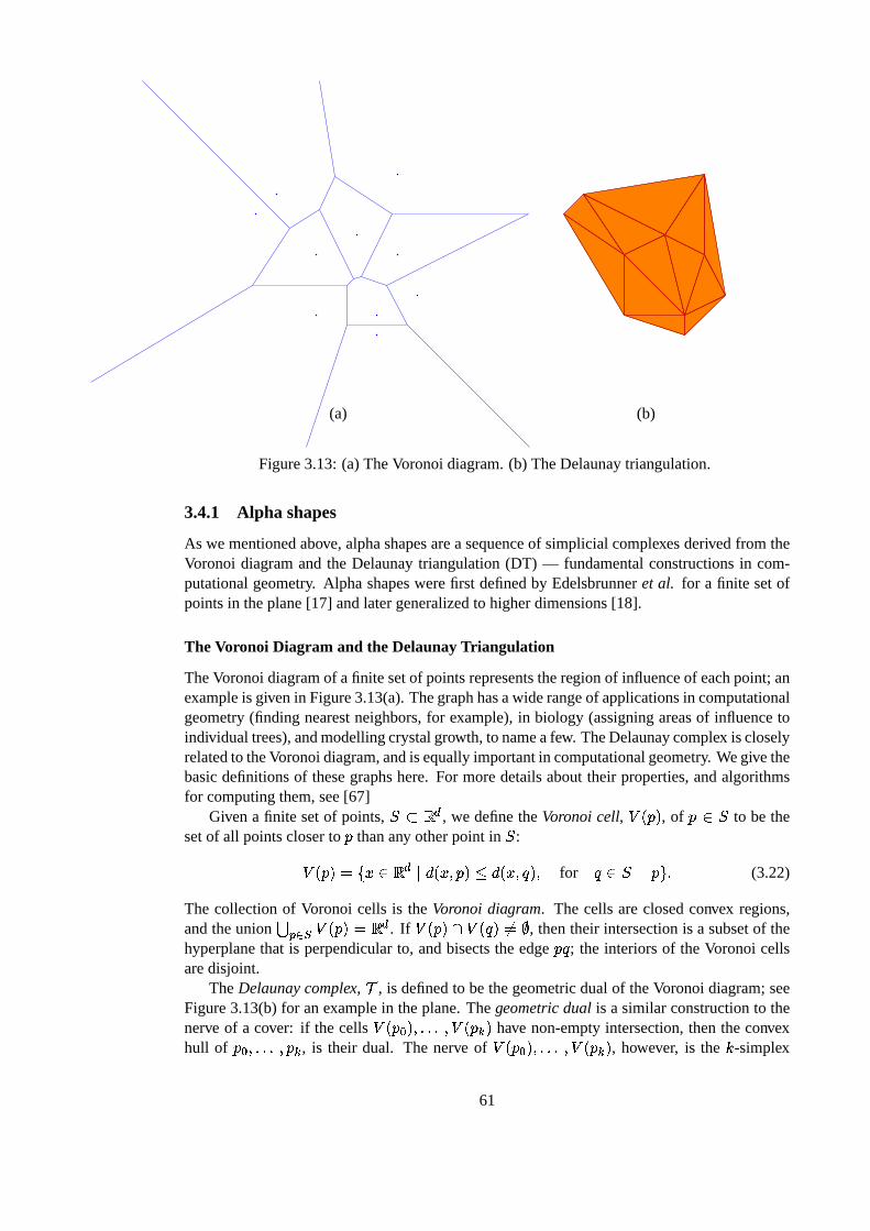
Figure3.13:(a) TheVoronoidiagram.(b) TheDelaunaytriangulation.

3.4.1 Alpha shapes

As we mentionedabove,alphashapesareasequenceof simplicial complexesderivedfrom theVoronoi diagramandthe Delaunaytriangulation(DT) — fundamentalconstructionsin com-putationalgeometry. Alpha shapeswerefirst definedby Edelsbrunneret al. for a finite setofpointsin theplane[17] andlatergeneralizedto higherdimensions[18].

The Voronoi Diagram and the DelaunayTriangulation

TheVoronoidiagramof afinite setof pointsrepresentstheregionof influenceof eachpoint;anexampleis givenin Figure3.13(a).Thegraphhasawiderangeof applicationsin computationalgeometry(finding nearestneighbors,for example),in biology (assigningareasof influencetoindividualtrees),andmodellingcrystalgrowth, to nameafew. TheDelaunaycomplex iscloselyrelatedto theVoronoidiagram,andis equallyimportantin computationalgeometry. Wegivethebasicdefinitionsof thesegraphshere. For moredetailsabouttheir properties,andalgorithmsfor computingthem,see[67]

Givena finite setof points, �W?A�þ , we definetheVoronoi cell, ö � Ö �, of Ö Q � to bethe

setof all pointscloserto Ö thanany otherpoint in � :ö � Ö �G��� Q A þ �9������ Ö �Ð�\�]��­���g�:�for

� Q ��HV֭��� (3.22)

The collectionof Voronoi cells is the Voronoi diagram. The cells areclosedconvex regions,andtheunion R í5SUT ö � Ö �Ð� A þ . If ö � Ö � K ö ���g�+%�WV

, thentheir intersectionis a subsetof thehyperplanethat is perpendicularto, andbisectstheedgeÖ � ; the interiorsof theVoronoi cellsaredisjoint.

TheDelaunaycomplex, X , is definedto bethegeometricdualof theVoronoidiagram;seeFigure3.13(b)for anexamplein theplane.Thegeometricdual is a similar constructionto thenerve of a cover: if thecells ö � Ö 8=�:� �>�>� � ö � Ö 3 � have non-emptyintersection,thentheconvexhull of Ö 8�� �>�>� � Ö 3 , is their dual. The nerve of ö � Ö 8��:� �>�>� � ö � Ö 3 � , however, is the 1 -simplex

61

c

b

d

a

a

c

d

b

Figure3.14: The points, ' �)(=� * �:� arenot in generalpositionbecausethey simultaneouslylieon a circle. Thefour Voronoicells intersectat thecenterof this circle which meanstheDelau-nay complex containsthe quadrilateral' ( * � . The nerve of the Voronoi complex containsthetetrahedron, ' ( * �t- ., Ö 8 � �>�>� � Ö 3 - — thedifferenceis illustratedin Figure3.14.In thisexample,four cellsintersectata point,sothegeometricdualis aquadrilateral,whereasthenerve containsa tetrahedron.Thissituationis adegenerateone;it only occurswhenfour pointssimultaneouslylie on acircle. Toexcludethis degeneracy, thepointsin � aretypically assumedto be in general position. Thisimposestheconditionthatno

��� 57D � pointsin � lie on theboundaryof a�-sphere(wediscuss

the practicalityof this assumptionlater). When � satisfiesthe generalposition condition,apoint in AGþ canbelongto atmost

� 5T+ differentVoronoicellsandit follows thattheDelaunaycomplex is a simplicial complex. This is why theDelaunaycomplex is usuallyreferredto astheDelaunaytriangulation. Note that theunderlyingspaceof theDelaunaycomplex,

� X �, is

theconvex hull of � .A consequenceof theabove discussionis thatwhenthepointsarein generalposition,the

Delaunaytriangulationis a geometricrealizationof the nerve of the Voronoi diagram. Thiscorrespondenceis usedto definethealphacomplexes.

Alpha complexes

Wenow describehow EdelsbrunnerintroducestheresolutionparameterY into theVoronoidia-gramandDelaunaytriangulation.Thisoperationgeneratesasequenceof simplicial complexesthat triangulatethe Y -neighborhoodsof thedataset � . TheparameterY is exactly thesameasourparameter� ; we switchto Y in this sectionto beconsistentwith theoriginalpapers.

TheclosedY -neighborhood�@Z is just theunionof all closedballsof radius Y with centersin � : � Z �\[í5SUT p Z � Ö �:�

where p Z � Ö �d� ������]��­� Ö ��� YG���These Y -balls thereforeform a cover of � Z . We could take the nerve of this cover, but thecorrespondingsimplicial complex is likely to have simplicesof a higherdimensionthan the

62

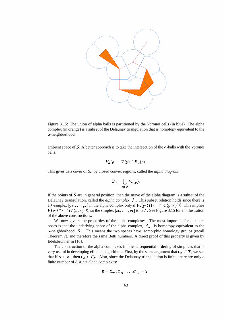
Figure3.15: Theunionof alphaballs is partitionedby theVoronoi cells (in blue). Thealphacomplex (in orange)is asubsetof theDelaunaytriangulationthatis homotopy equivalentto theY -neighborhood.

ambientspaceof � . A betterapproachis to take theintersectionof the Y -ballswith theVoronoicells: ö Z � Ö ��� ö � Ö � K p Z � Ö � �Thisgivesusacover of � Z by closedconvex regions,calledthealphadiagram:� Z � [í5SUT ö Z � Ö � �If thepointsof � arein generalposition,thenthenerve of thealphadiagramis a subsetof theDelaunaytriangulation,calledthealphacomplex, F Z . This subsetrelationholdssincethereisa 1 -simplex , Ö 89� �>�>� � Ö 3 - in thealphacomplex only if ö Z � Ö 8�� K }>}>} K ö Z � Ö 3 �&%�]V

. This impliesö � Ö 8�� K }>}>} K ö � Ö 3 �^%�]V, sothesimplex , Ö 89� �>�>� � Ö 3 - is in X . SeeFigure3.15for anillustration

of theabove constructions.We now give somepropertiesof the alphacomplexes. The most importantfor our pur-

posesis that the underlyingspaceof the alphacomplex,� F_Z �

, is homotopy equivalent to theY -neighborhood,� Z . This meansthe two spaceshave isomorphichomologygroups(recallTheorem7), andthereforethesameBetti numbers.A directproof of this propertyis givenbyEdelsbrunnerin [16].

Theconstructionof thealphacomplexesimpliesa sequentialorderingof simplicesthat isveryusefulin developingefficientalgorithms.First,by thesameargumentthat F Z ?`X , weseethat if Ya"]Y Ê , then F Z ?iF Z5b . Also, sincetheDelaunaytriangulationis finite, thereareonly afinite numberof distinctalphacomplexes:VI� F Zdc � F Z ï � �>�>� � F Zde � X �

63

Theseareorderedby increasingY , andby convention, Y 8�� % and F 8��fV. This ordering

of the alphacomplexes inducesan orderingof the simplicesin X . If 2 8�� 2 ;=� �>�>� � 2hg b is theorderedlist of simplicesin F Zdi , then 2 g b n ; � �>�>� � 2 g b nbê arethe ì simplicesin F Z i îcï HVF Zdi , listedin orderof increasingdimension. This sequentialorderingof simplicesis calleda filter andthe correspondingsequenceof complexes is a filtration. The algorithmfor determiningthisorderingis basedon computingtheradiusof thecircumsphereof eachsimplex in X ; see[18]for details.

DelfinadoandEdelsbrunner’s algorithm[11] for computingtheBetti numbersof a simpli-cial complex relieson this sequentialorderingof simplices.The theoreticalunderpinningsoftheir algorithmcomefrom centralresultsin homologytheorysuchasthe Mayer-Vietoris se-quenceandPoincare duality. TheBetti numbersarecomputedincrementallyaseachsimplexis addedto thecomplex. This processdependson a testto determinewhetherthenew simplexbelongsto a 1 -cycle of the new complex. Thereareefficient algorithmsfor testing1-cycles,andhomology-cohomologyduality theoremstransformthe

��� Hi+ � -cyclesinto 1-cocyclesthatare equally easyto test for. However, thereis no test for other 1 -cycles, so DelfinadoandEdelsbrunner’s algorithmappliesonly to subcomplexesof A x or Ae� .

Remarks

TheNCSAftp siteprovidessoftwarethatimplementsall of theabovealphashapeconstructionsin A x and Ae� [1]. WegeneratetheBetti numberdatafor theexamplesin Section3.5usingthissoftware. TheNCSA alphashapesoftwarerequiresthe input data, � , to be in integer format.This reducessomeof the standardproblemswith datastructuresin computationalgeometry.The implementationusesa techniqueof simulatedperturbationsto copewith any degenera-cies,sotherestrictionthat thepointsof � be in generalpositionis removed[18]. Complexityboundsfor thealgorithmsinvolved areat worstquadraticin thenumberof points, 0 , for bothtime andstorage.The Delaunaytriangulationof a setof points in the planecanbe found inN � 0¿ß>254Ð0 �

timeand N � 0 �storage.For asubsetof A � , theNCSAsoftwareusesanincremental

flip algorithmwhich builds thecomplex in N � 0 x � time andstorage.Thesimplicesof theDe-launaytriangulationarethensortedby the radiusof their circumsphere;this processrequiresN � �hß>254Ð� �

time,where� is thenumberof simplices.Theincrementalalgorithmfor comput-ing theBetti numbertakes N � �jY � � ���

to find all Betti numbersfor all thealphacomplexesofasubsetof AG� , andis slightly fasterfor subsetsof A x . Thefunction Y � � �

is theinverseof Ack-ermann’s function(which is definedby repeatedexponentiation)andit thereforehasextremelyslow growth. This timeestimateis commonin algorithmsinvolving setoperations;see[9].

TheNCSA alphashapeimplementationgoesa long way towardscarryingout our desiredprogram.It is not clearhow to easilyincorporatethecomputationof persistentBetti numbers.It is possiblethatanincrementalalgorithmfor finding thepersistentBetti numbersexists,asisthecasefor the regularBetti numbers.However, finding thepersistentBetti numbersrequiressomeexplicit informationaboutthecyclesandboundaries,andthealphashapealgorithmdoesnotgenerateor recordthis information.This problemclearlyrequiresfurtherwork.

Anotherdrawbackof thealphashapealgorithmis a largedegreeof redundancy in thetrian-gulationsfor thetypeof datawe areinterestedin. TheDelaunaytriangulationbuilds simplicesthat involve every singledatapoint, and this generatesa much finer complex than is neces-sary for resolutions�§U � . This redundancy is likely to occurwhenever we constructF � � asa subcomplex of F �3O

for � O "B� ê . In Section3.4.3,we discussa possiblealternative approachto building complexeson multiple scalesbasedon subdivisions. In the following section,weoutlinesomeotherfastalgorithmsfor computingBetti numbersof asinglecomplex.

64

3.4.2 Other algorithms for computational homology

Thedevelopmentof fastalgorithmsfor computationalhomologyis anactive areaof research.Many differentapproachesexist for variousspecificapplications,mostly for complexesin Ae� .To thebestof our knowledge,thealphashapealgorithmis theonly onethatgivesinformationat multiple resolutions. In this section,we give a very brief overview of someof the recentliterature.

Dey andGuha[14] describeanefficientalgorithmfor computingBetti numbersandgeomet-ric representationsof thenon-boundingcyclesfrom 3-manifoldsin Ae� . They thengeneralizethis to includeany simplicial complex in Ae� througha processof thickening. They areinter-estedin applicationsto solidmodelling,molecularbiologyandcomputer-aidedmanufacturing.This algorithmfindstheBetti numberswith time andstoragecomplexity thatarelinear in thesizeof thecomplex, andthegeneratorsfor thefirst andsecondhomologygroupswith acostoforder N � 0 x ¥��

in time,where¥

is themaximumgenusof theboundarysurfaces.In [37] Kaliesetal. developanalgorithmfor computingtheBetti numbersfrom cubicalcell

complexes.Theirapproachis basedon a local reductionof thecomplex to simplerform. In A xthis reductionis ahomotopy equivalenceandtheresultof thereductionsis a minimal complexconsistingof loops.Thenumberof loopsgivesthefirst Betti number. In higherdimensions,thereducedcomplex maynotbeminimalandthereductionstepsareno longersimplehomotopies.Kalieset al. conjecturethat theBetti numberscanbecomputedwith N � 0¿ß3254 � 0 �

operations,where 0 is the numberof cubesin thecomplex. This codewasdevelopedfor applicationsindynamicalsystems— specifically, for computingtheConley index of isolatingneighborhoodsof invariant setsfor flows generatedby ODEs; see[58] for an example. The generationofcubicalcoversof suchsetsis part of the GAIO (global analysisof invariantobjects)project[12] and is an efficient way to representsuccessive approximationsto attractorsor unstablemanifolds,for example.

Finally, we describeanapproachdueto Friedman[26] which computestheBetti numbersof arbitrarysimplicialcomplexesin A þ . Thismethodis basedonafundamentalresultof Hodgetheorywhich saysthat thehomologygroups(with realor rationalcoefficients)areisomorphicto thenull spaceof aLaplacianoperatoronthechaincomplexes.TheLaplacian,k 3ZY K 3 # K 3is formedfrom theboundaryoperatorsandtheir transposes:k 3 � X 3>n ; X Ï3�n ; 5~X Ï3 X 3 �Hodgetheoryimplies that the 1 th Betti numberis thedimensionof thenull spaceof k 3 . Forsimplicial complexes, Friedmanconstructsa matrix representationof the Laplaciandirectly,without using the boundaryoperatorsexplicitly. The matrix for k 3 is positive semidefiniteandsymmetric,andtypically quite sparse,so it is amenableto fastalgorithmsfor computingranksandnull spaces.To computethedimensionof thenull space,Friedmanmakesa carefulapplicationof thepower methodfor finding eigenvaluesandeigenvectors.Thepower methodcanbe inaccuratefor large matriceswith repeatedeigenvalues;Friedman’s methodattemptsto rigorouslyverify the correctnessof the computedBetti numbers.This algorithmholdsforsimplicial complexesof any finite dimensionandtherunningtime is approximatelyquadraticin thenumberof simplices.See[26] for detailedcomplexity bounds.

3.4.3 A better way?

The two main drawbacksto the alphashapeimplementationare(1) that the simplicial com-plexesarefiner thanthey needto be,and(2) the fastalgorithmfor computingBetti numbers

65

only holds in A x and A � . The excessive numberof simplicesin the alphacomplexesmeansthat computingthe persistentBetti numbersfrom the formula in Section3.3.5 is unrealistic.Any subcomplex approachto generatinga sequenceof complexesat differentresolutionswillencounterthe sameproblemof having an unnecessarilylarge numberof simplicesat coarserresolutions.Theremainderof this sectionsketchesanalternative approachto generatingcom-plexesat multiple resolutionsbasedon subdivisions.

Theadvantageof subdivisionsis thatcomplexesat coarseresolutionshave fewer simplicesthanthoseat fine resolutions.Subdivision of simplicial complexesis a commonprocess,bothin homologytheoryandin computationalgeometry. For applicationsto generalscatteredpointdata,however, cubicalcomplexesarea morenaturalconstruction.Thecubicalcomplexeswehave in mind areessentiallyregularmeshesin AGC . Thelevel-0complex is asinglecube

� F 8�� Q� , with side * . This cubeis thensubdivided into D C equalcubesof side * s D , andthe level-1complex, F ;

, consistsof thosecubesthat containa point from � . This processis repeatedonthecubesof F ;

to get F x , andsoon. Thesequenceof complexescanbeorganizedinto a treestructure;suchamultiresolutioncubicalcomplex is usuallyreferredto asaquadtreein A x , andanoctreeAe� .

Thissequenceof cubicalcomplexesdoesnothaveascloseacorrespondencewith � -neighborhoodsasthealphacomplexesdo,sowe needto slightly modify theinversesystemsof Section3.3.1.Givena compactspace

� ?iAGC , it is possibleto constructa sequenceof cubicalcomplexesaswedescribedin theprevioussection.Theunderlyingspace,

� F O �, of suchacubicalcomplex still

hasthehomotopy typeof afinite polyhedron;� F O � # �

in theHausdorff metric;andfor Ä � ì ,F Ois a refinementof F ê . Thesepropertiesshouldbeenoughto show that the resultinginverse

systemof homologygroupsis isomorphicto Cechhomology.

Anothersubstantialdifferencebetweenthe subdivision andsubcomplex approachesis inthe chain mapsinducedby inclusion on the underlyingspaces. For the sequenceof alphacomplexes,thesechainmapsareone-to-oneinclusionmapson thecomplexes.For thecubicalcomplexes,if F O

is a subdivision of F ê , we still have that� F O � ? � F ê �

. Thechainmaps� Í areno

longerone-to-one,however, sinceeachcubein F ê is subdivided into D�C cubes,andall of thesearepossiblyin F O

. The inclusion-inducedchain map thereforemapsall of thesecubesontothelargerone.Thishasimplicationsfor thenumericalimplementationof computingpersistentBetti numbers.

Of all the fastBetti numbercomputationsdescribedearlier, it seemsthat Friedman’s ap-proachusingtheLaplacianhasthemostpotentialfor adaptationto our proposedsubcomplexapproach.Theisomorphismbetweenhomologygroupsandthenull spaceof aLaplacianmatrixsuggeststhat in orderto computepersistentBetti numbers,we needonly find intersectionsofnull spacesof the appropriateLaplacianmatrices. This is an easiernumericallinear algebraproblemthanthe oneimplied by the formula in Section3.3.5. Therearestill problemsto beworkedthroughhere.In particular, how to build theLaplacianmatrix from cubicalcomplexes(ratherthansimplicialones),andhow to incorporatetheinclusion-inducedchainmapsbetweentheLaplaciannull spaces.

The above ideasare just onepossibledirection for the developmentof moreefficient al-gorithmsto computepersistentBetti numbersfrom data. This an openproblemthat needsasubstantialamountof furtherwork.

66

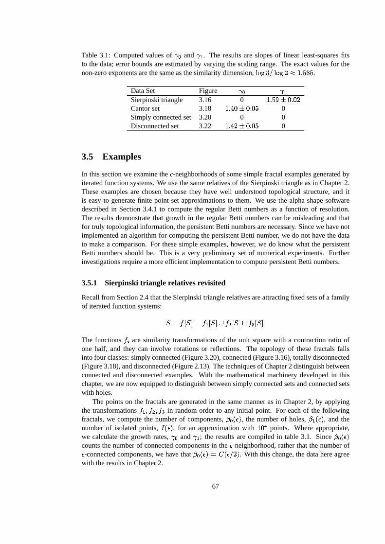
Table3.1: Computedvaluesof - 8 and - ; . The resultsareslopesof linear least-squaresfitsto thedata;errorboundsareestimatedby varying thescalingrange.Theexact valuesfor thenon-zeroexponentsarethesameasthesimilarity dimension,ß3254ýE s ß3254�D 8 +9�l<5m5< .

DataSet Figure - 8 - ;Sierpinskitriangle 3.16 0 +9�l<5n�o7%c��%�DCantorset 3.18 +9�p:�%�o7%c��%d< 0Simplyconnectedset 3.20 0 0Disconnectedset 3.22 +9�p:½D&o7%c��%d< 0

3.5 Examples

In this sectionwe examinethe � -neighborhoodsof somesimplefractalexamplesgeneratedbyiteratedfunctionsystems.We usethesamerelativesof theSierpinskitriangleasin Chapter2.Theseexamplesare chosenbecausethey have well understoodtopologicalstructure,and itis easyto generatefinite point-setapproximationsto them. We usethe alphashapesoftwaredescribedin Section3.4.1 to computethe regular Betti numbersasa function of resolution.The resultsdemonstratethat growth in the regular Betti numberscanbe misleadingandthatfor truly topologicalinformation,thepersistentBetti numbersarenecessary. Sincewehavenotimplementedanalgorithmfor computingthepersistentBetti number, we do not have thedatato make a comparison.For thesesimpleexamples,however, we do know what the persistentBetti numbersshouldbe. This is a very preliminary set of numericalexperiments. Furtherinvestigationsrequireamoreefficient implementationto computepersistentBetti numbers.

3.5.1 Sierpinski triangle relativesrevisited

Recallfrom Section2.4thattheSierpinskitrianglerelativesareattractingfixedsetsof a familyof iteratedfunctionsystems: � � ¤G,�� -<� ¤ ; ,�� -jé ¤ x ,�� -cé ¤ � ,�� - �The functions ¤ O aresimilarity transformationsof the unit squarewith a contractionratio ofone half, and they can involve rotationsor reflections. The topology of thesefractals fallsinto four classes:simplyconnected(Figure3.20),connected(Figure3.16),totally disconnected(Figure3.18),anddisconnected(Figure2.13).Thetechniquesof Chapter2 distinguishbetweenconnectedand disconnectedexamples. With the mathematicalmachinerydevelopedin thischapter, wearenow equippedto distinguishbetweensimplyconnectedsetsandconnectedsetswith holes.

The pointson the fractalsaregeneratedin the samemannerasin Chapter2, by applyingthe transformations¤ ; � ¤ x � ¤ � in randomorder to any initial point. For eachof the followingfractals,we computethe numberof components,� 8t� � � , the numberof holes, � ;�� � � , and thenumberof isolatedpoints, q � � � , for an approximationwith +>% � points. Whereappropriate,we calculatethe growth rates, - 8 and - ; ; the resultsarecompiledin table3.1. Since � 8�� � �countsthenumberof connectedcomponentsin the � -neighborhood,ratherthat thenumberof� -connectedcomponents,we have that � 8t� � ��� K � � s D �

. With this change,thedatahereagreewith theresultsin Chapter2.

67

The Sierpinski triangle

Thegeneratingfunctionsfor theSierpinskitriangleare:¤ ;������rÎ�G� ;x ��­��r��¤ x �����rÎ�G� ;x �� 5h+ ��rÎ�¤ � �����rÎ�G� ;x ��­��r 5P+ � � (3.23)

A finite point-setapproximationto thetriangle,an � -neighborhoodandthecorrespondingsubsetof the Delaunaytriangulationare shown in Figure 3.16. The underlyingset is perfectandconnectedwith infinitely many holes,sowe shouldsee� 8t� � ��� + and � ;�� � � #s( as �¿#°% .As wederivedin Section3.2.4,for

¾ 8 %c�`+�:�; ,¾ s D C "i� C " ¾ s D C [ ; �� ; � � C �d� C^3 _ ; E 3 � ;x � E C H\+ � �Thegrowth rate, - ;l� ß>254ÐE s ß3254lD 8 +9�l<5m5< , is thesameasthesimilarity dimension.

Theseexpectedresultsarereflectedby thecomputationsof � 8t� � � , � ;�� � � and q � � � (graphedin Figure 3.17) for the +>% � point approximationto the triangle. We seethat for � above athresholdvalue,thecomputedvaluesof � 8 � � � and � ; � � � arein closeagreementwith thetheory.The point at which � 8t� � � and � ;�� � � “blur” is approximately� � %c��%t%�E , closeto the valueatwhich the numberof isolatedpoints, q � � � , becomespositive. This � value is, of course,thecutoff resolution� . As wesaw in Chapter2, atfiner resolutions— i.e., �^"~� — thereis asharptransitionin thegraphof � 8

from oneto thenumberof pointsin theset,aseachpoint becomesisolated.Thegraphof � ;

shows thattheholesaredestroyedas � decreases.This is becausetheedgesthat form theloopsareeventuallydeletedfrom thetriangulation.We estimatetheslopeof thestaircaseby a linear, least-squaresfit andfind - ; 8 +9�l<5n . This is very closeto thevaluederivedabove.

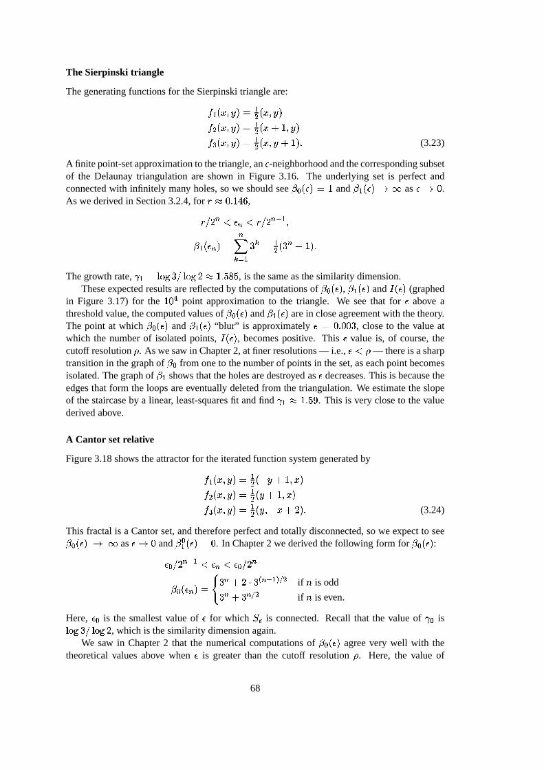
A Cantor setrelative

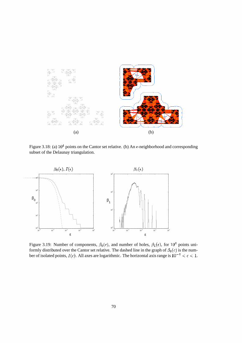
Figure3.18shows theattractorfor theiteratedfunctionsystemgeneratedby¤ ;������rÎ�G� ;x � H r 5P+ �:4�¤ x �����rÎ�G� ;x ��r 5h+ �:4�¤ � �����rÎ�G� ;x ��r�� H 5~D � � (3.24)

This fractal is a Cantorset,andthereforeperfectandtotally disconnected,sowe expectto see� 8t� � � # ( as ��#À% and � 8; � � �d� % . In Chapter2 we derivedthefollowing form for � 8t� � � :� 8 s D C n ; "i� C "i� 8 s D C� 8 � � C ���ut E�C�5~D } E�v�C [ ;1w�x x if 0 is oddE C 5~E C x x if 0 is even.

Here, � 8 is the smallestvalueof � for which � �is connected.Recall that the valueof - 8 isß3254�E s ß3254ýD , which is thesimilarity dimensionagain.

We saw in Chapter2 that the numericalcomputationsof � 8t� � � agreevery well with thetheoreticalvaluesabove when � is greaterthan the cutoff resolution � . Here, the value of

68

(a) (b)

Figure3.16:(a) +>% � pointsontheSierpinskitriangle.(b) An � -neighborhood(blueoutline)andcorrespondingsubsetof theDelaunaytriangulation(orange).

� 8 � � � , q � � � � ; � � �

10−4

10−3

10−2

10−1

100

100

101

102

103

104

ε

β0

10−4

10−3

10−2

10−1

100

100

101

102

103

ε

β1

Figure3.17: Numberof components,� 8t� � � , andnumberof holes, � ;�� � � , for +>% � pointsuni-formly distributedovertheSierpinskitriangle.Thedashedline in thegraphof � 8t� � � is thenum-berof isolatedpoints,q � � � . All axesarelogarithmic.Thehorizontalaxisrangeis +>% [ � "i�"W+ .

69

(a) (b)

Figure3.18:(a) +>% � pointsontheCantorsetrelative. (b) An � -neighborhoodandcorrespondingsubsetof theDelaunaytriangulation.

� 8 � � � , q � � � � ; � � �

10−4

10−3

10−2

10−1

100

100

101

102

103

104

ε

β0

10−4

10−3

10−2

10−1

100

100

101

102

103

ε

β1

Figure3.19: Numberof components,� 8t� � � , andnumberof holes, � ;�� � � , for +>% � pointsuni-formly distributedover theCantorsetrelative. Thedashedline in thegraphof � 8t� � � is thenum-berof isolatedpoints,q � � � . All axesarelogarithmic.Thehorizontalaxisrangeis +>% [ � "i�"W+ .

70

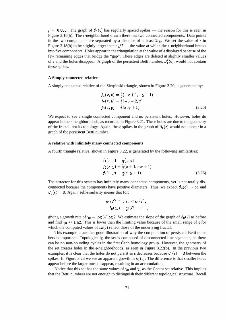
� 8 %c��%t%d< . The graphof � ;�� � � hasregularly spacedspikes— the reasonfor this is seeninFigure3.18(b). The � -neighborhooddrawn therehastwo connectedcomponents.Datapointsin the two componentsareseparatedby a distanceof at least Dt� 8 . We set the valueof � inFigure3.18(b)to beslightly larger than � 8 s D — thevalueat which the � -neighborhoodbreaksinto fivecomponents.Holesappearin thetriangulationatthevalueof � displayedbecauseof thefew remainingedgesthatbridgethe “gap”. Theseedgesaredeletedat slightly smallervaluesof � andtheholesdisappear. A graphof thepersistentBetti number, � ?; � � � , would not containthesespikes.

A Simply connectedrelative

A simply connectedrelative of theSierpinskitriangle,shown in Figure3.20,is generatedby:¤ ;=�����rÎ��� ;x � H 5P+ � H r 5h+ �¤ x �����rÎ��� ;x � H r 5\D �:4�¤ � �����rÎ��� ;x ��­��r 5P+ � � (3.25)

We expect to seea singleconnectedcomponentandno persistentholes. However, holesdoappearin the � -neighborhoods,asrecordedin Figure3.21.Theseholesaredueto thegeometryof thefractal,not its topology. Again, thesespikesin thegraphof � ;�� � � would not appearin agraphof thepersistentBetti number.

A relative with infinitely many connectedcomponents

A fourth trianglerelative,shown in Figure3.22,is generatedby thefollowing similarities:¤ ;=�����rÎ��� ;x ��­��r��¤ x �����rÎ��� ;x ��r 5h+ � H 5P+ �¤ � �����rÎ��� ;x ��­��r 5P+ � � (3.26)

Theattractorfor this systemhasinfinitely many connectedcomponents,yet is not totally dis-connectedbecausethecomponentshave positive diameters.Thus,we expect � 8t� � � #s( and� 8; � � ��� % . Again,self-similaritymeansthatfor:� 8 s D C n ; "f� C "f� 8 s D C �� 8t� � C ��� ;x � E C n ; 5P+ �:�giving agrowth rateof - 8 � ß3254ÐE s ß3254lD . Weestimatetheslopeof thegraphof � 8 � � � asbeforeandfind - 8 8 +9�p:½D . This is lower thanthe limiting valuebecauseof the small rangeof � forwhich thecomputedvaluesof � 8t� � � reflectthoseof theunderlyingfractal.

This exampleis anothergoodillustrationof why thecomputationof persistentBetti num-bersis important. Topologically, the setis composedof disconnectedline segments,so therecanbe no non-boundingcyclesin the first Cechhomologygroup. However, the geometryofthe setcreatesholesin the � -neighborhoods,asseenin Figure3.22(b). In the previous twoexamples,it is clearthattheholesdo not persistas � decreasesbecause� ; � � �u� % betweenthespikes. In Figure3.23we seeanapparentgrowth in � ;�� � � . Thedifferenceis thatsmallerholesappearbeforethelargeronesdisappear, resultingin anaccumulation.

Noticethatthis sethasthesamevaluesof - 8 and - ; astheCantorsetrelative. This impliesthattheBetti numbersarenotenoughto distinguishtheirdifferenttopologicalstructure.Recall

71

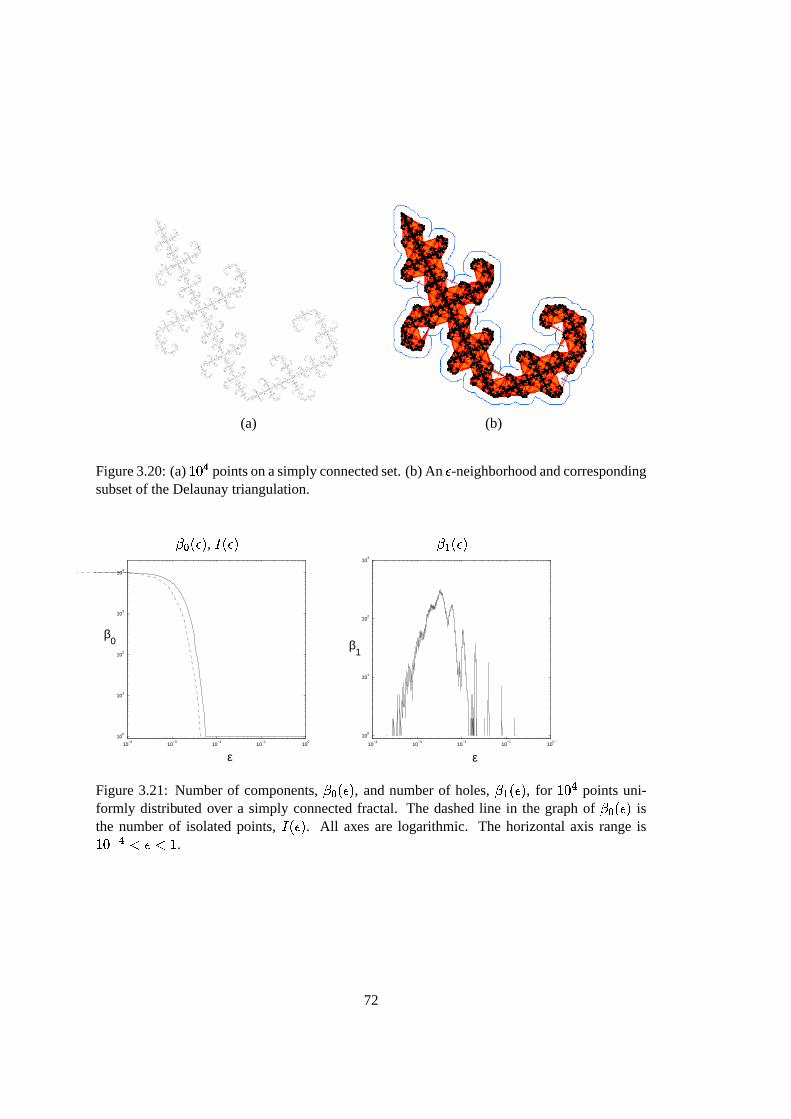
(a) (b)

Figure3.20:(a) +>% � pointsonasimplyconnectedset.(b) An � -neighborhoodandcorrespondingsubsetof theDelaunaytriangulation.

� 8t� � � , q � � � � ;=� � �

10−4

10−3

10−2

10−1

100

100

101

102

103

104

ε

β0

10−4

10−3

10−2

10−1

100

100

101

102

103

ε

β1

Figure3.21: Numberof components,� 8t� � � , andnumberof holes, � ;�� � � , for +>% � pointsuni-formly distributed over a simply connectedfractal. The dashedline in the graphof � 8 � � � isthe numberof isolatedpoints, q � � � . All axes are logarithmic. The horizontalaxis rangeis+>% [ � "i�&"W+ .

72

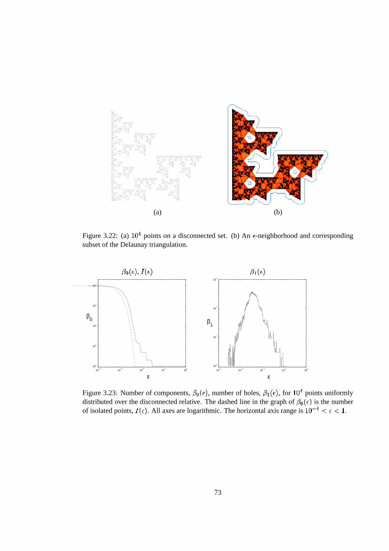
(a) (b)

Figure3.22: (a) +>% � pointson a disconnectedset. (b) An � -neighborhoodandcorrespondingsubsetof theDelaunaytriangulation.

� 8 � � � , q � � � � ; � � �

10−4

10−3

10−2

10−1

100

100

101

102

103

104

ε

β0

10−4

10−3

10−2

10−1

100

100

101

102

103

ε

β1

Figure3.23: Numberof components,� 8t� � � , numberof holes, � ;�� � � , for +>% � pointsuniformlydistributedover thedisconnectedrelative. Thedashedline in thegraphof � 8t� � � is thenumberof isolatedpoints, q � � � . All axesarelogarithmic.Thehorizontalaxisrangeis +>% [ � "i�^"W+ .

73

thatthiswasaddressedin Chapter2 by examiningthediametersof theconnectedcomponents.For a Cantorset, the diametersgo to zero,while for the examplein Figure3.22, the largestdiameterconvergesto one.

3.6 Concluding remarks

We have demonstratedthat it is possibleto extract informationaboutthe topologicalstructureof a compactspacefrom a finite approximationto it. The examplesgiven herearesubsetsof the planewhereit is easyto seethestructureof the data. In higher-dimensionalspaces,itis extremelydifficult visualizetheunderlyingtopologyof a cloudof points,socomputationaltechniquesbecomeevenmoreimportanttools.

In Section3.5,wecomputedonly theregularBetti numbers,� 3 � � � , of the � -neighborhoods.Theexamplesgivenhighlighttheneedfor computationof the � -persistentBetti numbers,� ?3 � � � .Thelattergiveabettercharacterizationof thetopologyof theunderlyingspace.In applications,both setsof numbersmay prove useful,sincethe Betti numbersof the � -neighborhoodsgivegeometricinformationabouthow theunderlyingspaceis embedded.

Many openproblemsremain. For the theoryof persistentBetti numbers,we needfurtherresultsrelatingthelimit of � Ñ3 �L���)�

asÙ

and � tendto zeroto theBetti numbersof�

. In termsof computation,morework canbedoneon developingandimplementingefficient algorithmsfor building complexesandcomputingpersistentBetti numbers.Fasteralgorithmsareessentialfor easein studyingthelargedatasetstypically encounteredin thestudyof dynamicalsystems.Weanticipatethatsuchcomputationaltoolswill assistin thenumericalinvestigationof chaoticsystemsby giving adeeperunderstandingof thestructureof attractorsandotherinvariantsets.

74