Embed Size (px)
Citation preview
8/6/2019 Computational Techniques for Tidal Datums Handbook
http://slidepdf.com/reader/full/computational-techniques-for-tidal-datums-handbook 1/113
U.S. DEPARTMENT OF COMMERCE
National Oceanic and Atmospheric Administration
National Ocean Service
Center for Operational Oceanographic Products and Services
COMPUTATIONAL TECHNIQUES
FOR
TIDAL DATUMS HANDBOOK
NOAA Special Publication NOS CO-OPS 2
8/6/2019 Computational Techniques for Tidal Datums Handbook
http://slidepdf.com/reader/full/computational-techniques-for-tidal-datums-handbook 2/113
Center for Operational Oceanographic Products and Services
The National Ocean Service (NOS) Center for Operational Oceanographic Products and
Services (CO-OPS) collects and distributes observations and predictions of water levels
and currents to ensure safe, efficient and environmentally sound maritime commerce. The
Center provides the set of water level and coastal current products required to support NOS'
Strategic Plan mission requirements, and to assist in providing operational oceanographic
data/products required by NOAA's other Strategic Plan themes. For example, CO-OPS
provides data and products required by the National Weather Service to meet its flood and
tsunami warning responsibilities. The Center manages the National Water Level
Observation Network (NWLON), and a national network of Physical Oceanographic Real-
Time Systems (PORTS®
) in major U.S. harbors. The Center: establishes standards for thecollection and processing of water level and current data; collects and documents user
requirements which serve as the foundation for all resulting program activities; designs
new and/or improved oceanographic observing systems; designs software to improve CO-
OPS' data processing capabilities; maintains and operates oceanographic observing
systems; performs operational data analysis/quality control; and produces/disseminates
oceanographic products.
8/6/2019 Computational Techniques for Tidal Datums Handbook
http://slidepdf.com/reader/full/computational-techniques-for-tidal-datums-handbook 3/113
NOAA Special Publication NOS CO-OPS 2
C0MPUTATIONAL TECHNIQUES FOR TIDALDATUMS HANDBOOK
Silver Spring, Maryland
September 2003
U.S. DEPARTMENT OF COMMERCEDon Evans, Secretary
National Oceanic and Atmospheric AdministrationConrad C. Lautenbacher, Jr.
Undersecretary of Commerce for Oceans and Atmosphere and NOAA Administrator
8/6/2019 Computational Techniques for Tidal Datums Handbook
http://slidepdf.com/reader/full/computational-techniques-for-tidal-datums-handbook 4/113
NOTICE
Mention of a commercial company or product does not constitute an endorsement
by NOAA. Use for publicity or advertising purposes of information from this
publication concerning proprietary products or the tests of such products is notauthorized.
8/6/2019 Computational Techniques for Tidal Datums Handbook
http://slidepdf.com/reader/full/computational-techniques-for-tidal-datums-handbook 5/113
TABLE OF CONTENTS
page
1. INTRODUCTION . . . . . . . . . . . . . . . . . . . . . . . . . . . . . . . . . . . . . . . . . . . . . . . . . . . . . . . 1
1.1 Intended Audience . . . . . . . . . . . . . . . . . . . . . . . . . . . . . . . . . . . . . . . . . . . . . . . 1
1.2 Statement of Philosophy . . . . . . . . . . . . . . . . . . . . . . . . . . . . . . . . . . . . . . . . . . . 1
1.3 Prerequisite Knowledge . . . . . . . . . . . . . . . . . . . . . . . . . . . . . . . . . . . . . . . . . . . 1
2. BACKGROUND . . . . . . . . . . . . . . . . . . . . . . . . . . . . . . . . . . . . . . . . . . . . . . . . . . . . . . . 3
2.1 Characteristics of the Tides . . . . . . . . . . . . . . . . . . . . . . . . . . . . . . . . . . . . . . . . 32.2 Lunitidal Interviews . . . . . . . . . . . . . . . . . . . . . . . . . . . . . . . . . . . . . . . . . . . . . . 7
2.3 Other Signals in Water Level Measurements . . . . . . . . . . . . . . . . . . . . . . . . . . . 7
2.4 Tide Station Networks . . . . . . . . . . . . . . . . . . . . . . . . . . . . . . . . . . . . . . . . . . . . 8
2.5 Bench Marks and Differential Leveling . . . . . . . . . . . . . . . . . . . . . . . . . . . . . . . 10
2.6 Data Processing Procedures . . . . . . . . . . . . . . . . . . . . . . . . . . . . . . . . . . . . . . . . 13
2.7 The National Tidal Datum Epoch . . . . . . . . . . . . . . . . . . . . . . . . . . . . . . . . . . . 16
3. GENERAL TIDAL DATUM COMPUTATION PROCEDURES3.1 Datum Computation Procedures Overview . . . . . . . . . . . . . . . . . . . . . . . . . . . . 19
3.2 Other Vertical Datums and Their Relationship to Tidal Datums . . . . . . . . . . . . 20
3.3 Steps required to Compute Tidal Datums at Short-term Stations . . . . . . . . . . . . 25
3.4 Datum Computation Methods . . . . . . . . . . . . . . . . . . . . . . . . . . . . . . . . . . . . . . . 25
Standard Method . . . . . . . . . . . . . . . . . . . . . . . . . . . . . . . . . . . . . . . . . . . . . . . . 25
Modified Range Ratio Method . . . . . . . . . . . . . . . . . . . . . . . . . . . . . . . . . . . . . . 26
Direct Method . . . . . . . . . . . . . . . . . . . . . . . . . . . . . . . . . . . . . . . . . . . . . . . . . . 26
3.5 Accuracy . . . . . . . . . . . . . . . . . . . . . . . . . . . . . . . . . . . . . . . . . . . . . . . . . . . . . . . 26
4. WORKED EXAMPLES OF TIDAL DATUMS . . . . . . . . . . . . . . . . . . . . . . . . . . . . . . . 31
4.1 Procedural Steps . . . . . . . . . . . . . . . . . . . . . . . . . . . . . . . . . . . . . . . . . . . . . . . . . 31
4.2 Comparison of Monthly Means . . . . . . . . . . . . . . . . . . . . . . . . . . . . . . . . . . . . . 31
4.2.1 Modified Range Ratio Method - Semidiurnal Tides . . . . . . . . . . . . . . . . 31
Definition, MTL . . . . . . . . . . . . . . . . . . . . . . . . . . . . . . . . . . . . . . . . . . . . 34
Definition, DTL . . . . . . . . . . . . . . . . . . . . . . . . . . . . . . . . . . . . . . . . . . . . 36Definition, Mn . . . . . . . . . . . . . . . . . . . . . . . . . . . . . . . . . . . . . . . . . . . . . 37
Definition, Gt . . . . . . . . . . . . . . . . . . . . . . . . . . . . . . . . . . . . . . . . . . . . . . 37
Definition, DHQ . . . . . . . . . . . . . . . . . . . . . . . . . . . . . . . . . . . . . . . . . . . 39
Definition, DLQ . . . . . . . . . . . . . . . . . . . . . . . . . . . . . . . . . . . . . . . . . . . . 39
4.2.2 Modified Range Ratio Method - Diurnal Tides . . . . . . . . . . . . . . . . . . . . 40

8/6/2019 Computational Techniques for Tidal Datums Handbook
http://slidepdf.com/reader/full/computational-techniques-for-tidal-datums-handbook 6/113
TABLE OF CONTENTS (cont.)
Corrected Mn at Alameda . . . . . . . . . . . . . . . . . . . . . . . . . . . . . . . . . . . . 51Definition, DHQ . . . . . . . . . . . . . . . . . . . . . . . . . . . . . . . . . . . . . . . . . . . 51
Definition, DLQ . . . . . . . . . . . . . . . . . . . . . . . . . . . . . . . . . . . . . . . . . . . . 52
4.3 Comparison of Simultaneous High and Low Waters . . . . . . . . . . . . . . . . . . . . . 54
4.3.1 Modified Range Ratio Method - Semidiurnal Tides . . . . . . . . . . . . . . . . 54
Type or Designation Conversion at Subordinate Station . . . . . . . . . . . . . 58
Tidal Datums . . . . . . . . . . . . . . . . . . . . . . . . . . . . . . . . . . . . . . . . . . . . . . 60
Lunitidal Intervals . . . . . . . . . . . . . . . . . . . . . . . . . . . . . . . . . . . . . . . . . . 65
4.3.2 Modified Range Ratio Method - Diurnal Tides . . . . . . . . . . . . . . . . . . . . 68Tidal Datums . . . . . . . . . . . . . . . . . . . . . . . . . . . . . . . . . . . . . . . . . . . . . . 71
Lunitidal Intervals . . . . . . . . . . . . . . . . . . . . . . . . . . . . . . . . . . . . . . . . . . 73
4.3.3 Standard Method - Mixed Tides . . . . . . . . . . . . . . . . . . . . . . . . . . . . . . . 75
Tidal Datums . . . . . . . . . . . . . . . . . . . . . . . . . . . . . . . . . . . . . . . . . . . . . . 77
Lunitidal Intervals . . . . . . . . . . . . . . . . . . . . . . . . . . . . . . . . . . . . . . . . . . 81
4.4 Direct Method . . . . . . . . . . . . . . . . . . . . . . . . . . . . . . . . . . . . . . . . . . . . . . . . . . . 83
5. SUMMARY and ACKNOWLEDGMENTS . . . . . . . . . . . . . . . . . . . . . . . . . . . . . . . . . . 90
6. REFERENCES . . . . . . . . . . . . . . . . . . . . . . . . . . . . . . . . . . . . . . . . . . . . . . . . . . . . . . . . . 97
Appendix 1: Example spreadsheets for semidiurnal and mixed tides . . . . . . . . . . . . . . . . . . A-1
Appendix 2: Relationships of tide and geodetic datums . . . . . . . . . . . . . . . . . . . . . . . . . . . . B-1

8/6/2019 Computational Techniques for Tidal Datums Handbook
http://slidepdf.com/reader/full/computational-techniques-for-tidal-datums-handbook 7/113
LIST OF FIGURES
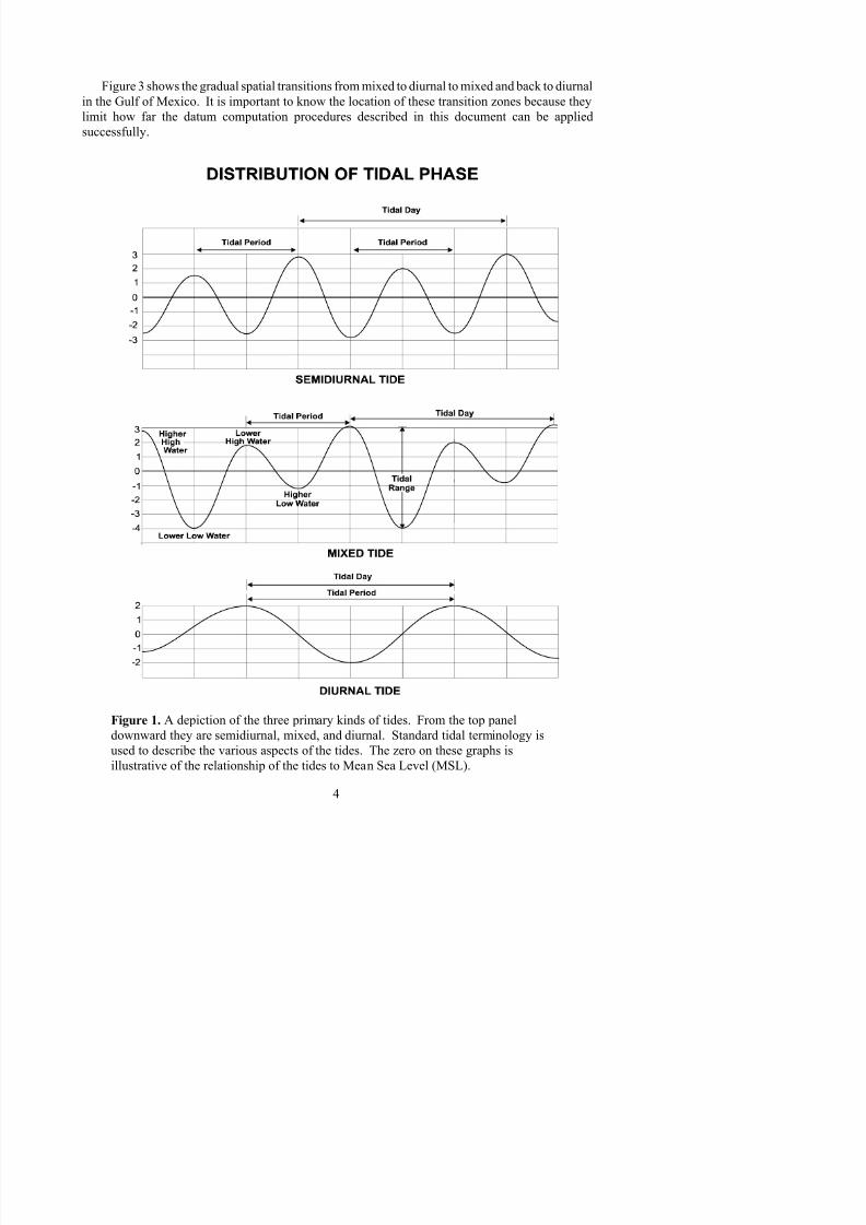
pageFigure 1. A depiction of the three primary kinds of tides. From the top panel downward they are
semidiurnal, mixed, and diurnal. Standard tidal terminology is used to describe the
various aspects of the tides. The zero on these graphs is illustrative of the relationship
of the tides to Mean Sea Level (MSL). . . . . . . . . . . . . . . . . . . . . . . . . . . . . . . . . . . 4
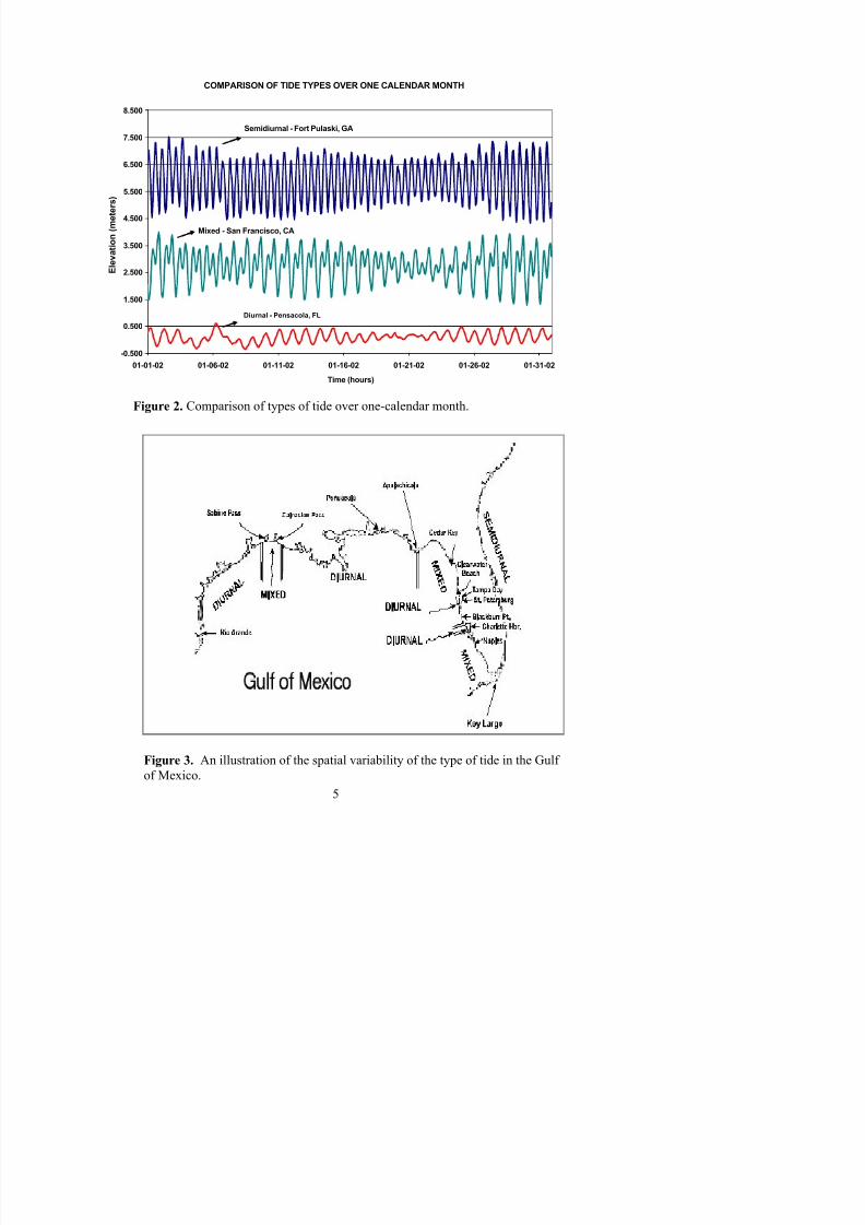
Figure 2. Comparison of types of tide over one calendar month . . . . . . . . . . . . . . . . . . . . . . 5
Figure 3. An illustration of the spatial variability of the type of tide in the Gulf of Mexico . 5
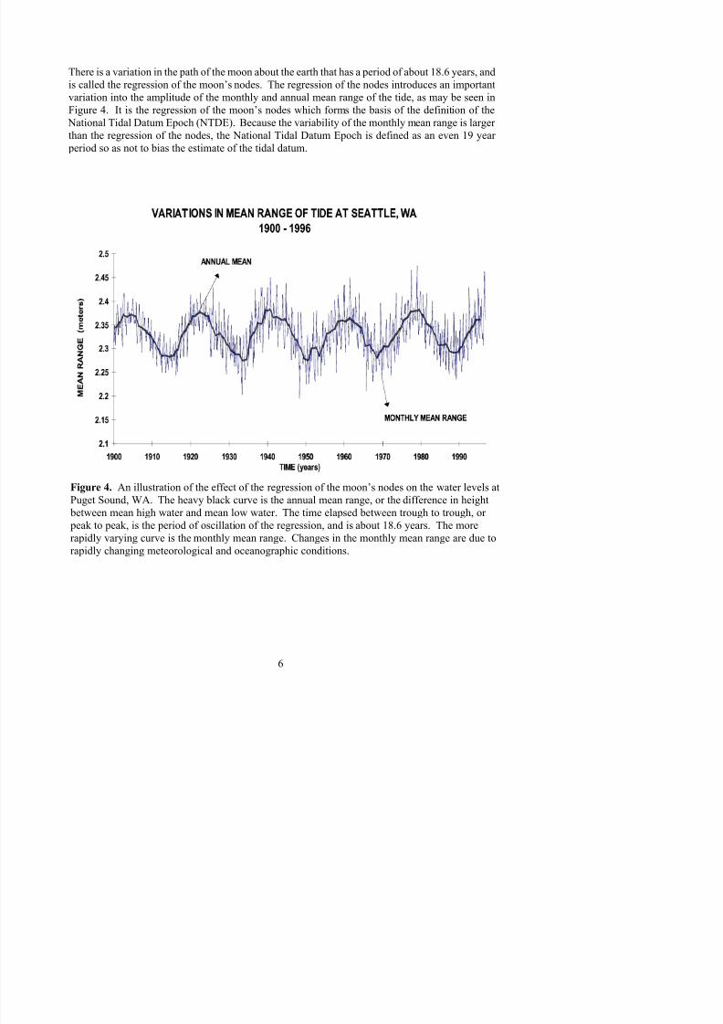
Figure 4. An illustration of the effect of the regression of the moon’s nodes on the water levels at
Puget Sound, WA. The heavy black curve is the annual mean range, or the difference
in height between mean high water and mean low water. The time elapsed between
trough to trough or peak to peak, is the period of oscillation of the regression, and is
about 18.6 years. The more rapidly varying curve is the monthly mean range. Changes
in the monthly mean range are due to rapidly changing meteorological and
oceanographic conditions . . . . . . . . . . . . . . . . . . . . . . . . . . . . . . . . . . . . . . . . . . . . 6
Figure 5. Locations of U.S. NWLON water level stations. . . . . . . . . . . . . . . . . . . . . . . . . . . . 9
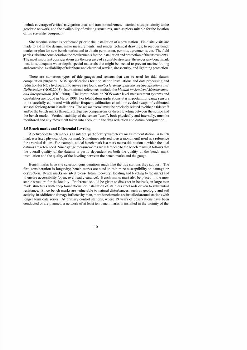
Figure 6. Illustration of the tide station network hierarchy. . . . . . . . . . . . . . . . . . . . . . . . . . 11
Figure 7. An schematic diagram of extending vertical control inland from the tidal datum by the
method of differential leveling. . . . . . . . . . . . . . . . . . . . . . . . . . . . . . . . . . . . . . . . . 13
Figure 8a and 8b. Observed 6-minute data for one-month and resulting tabulation of the tide 14
Figure 9. Example of a monthly tabulation of the tide. . . . . . . . . . . . . . . . . . . . . . . . . . . . . . . 15
Figure 10. Relative sea level change at several locations in the U.S. . . . . . . . . . . . . . . . . . . . . 17
Figure 11. Illustration of the long term changes in sea level causing the need to update tidal datumssuch as mean tide level (MTL). The graph shows the annual values of mean tide level
with horizontal lines drawn to show the 19-year MTL values for the 1941-59 and 1960-
78 NTDE. . . . . . . . . . . . . . . . . . . . . . . . . . . . . . . . . . . . . . . . . . . . . . . . . . . . . . . . . . 18
Figure 12 Tidal datums (1960-1978 NTDE) extreme water levels and geodetic elevations at
8/6/2019 Computational Techniques for Tidal Datums Handbook
http://slidepdf.com/reader/full/computational-techniques-for-tidal-datums-handbook 8/113
LIST OF FIGURES (cont.)
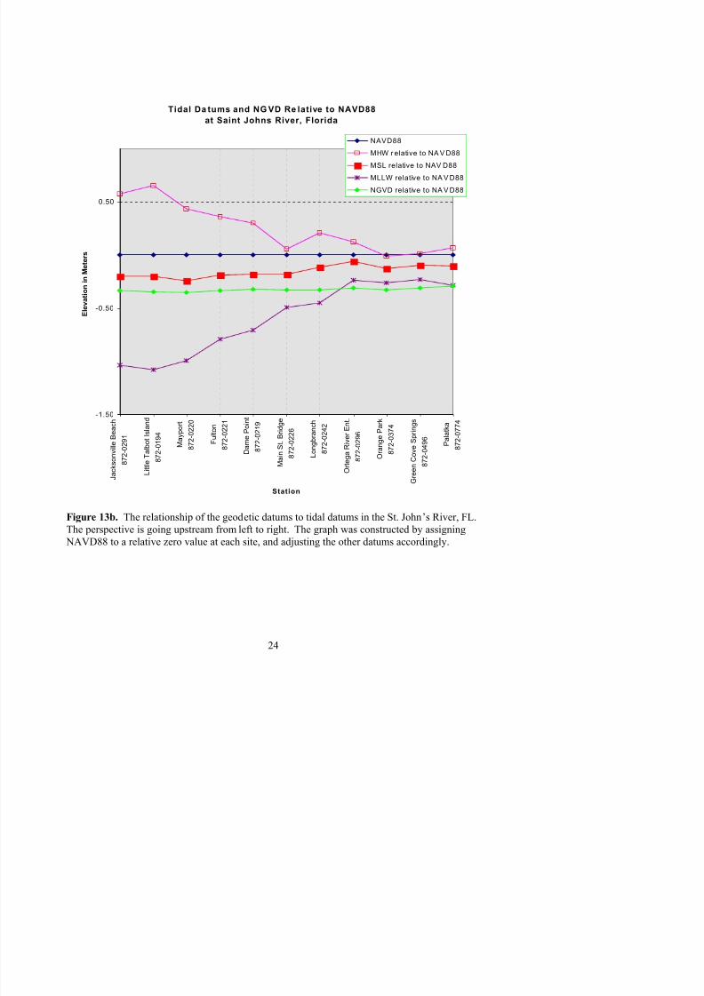
pageFigure 13b. The relationship of the geodetic datums to tidal datums in the St. John’s River, FL. The
perspective is going upstream from left to right. The graph was constructed by
assigning NAVD88 to a relative zero value at each site, and adjusting the other datums
accordingly. . . . . . . . . . . . . . . . . . . . . . . . . . . . . . . . . . . . . . . . . . . . . . . . . . . . . . . 24
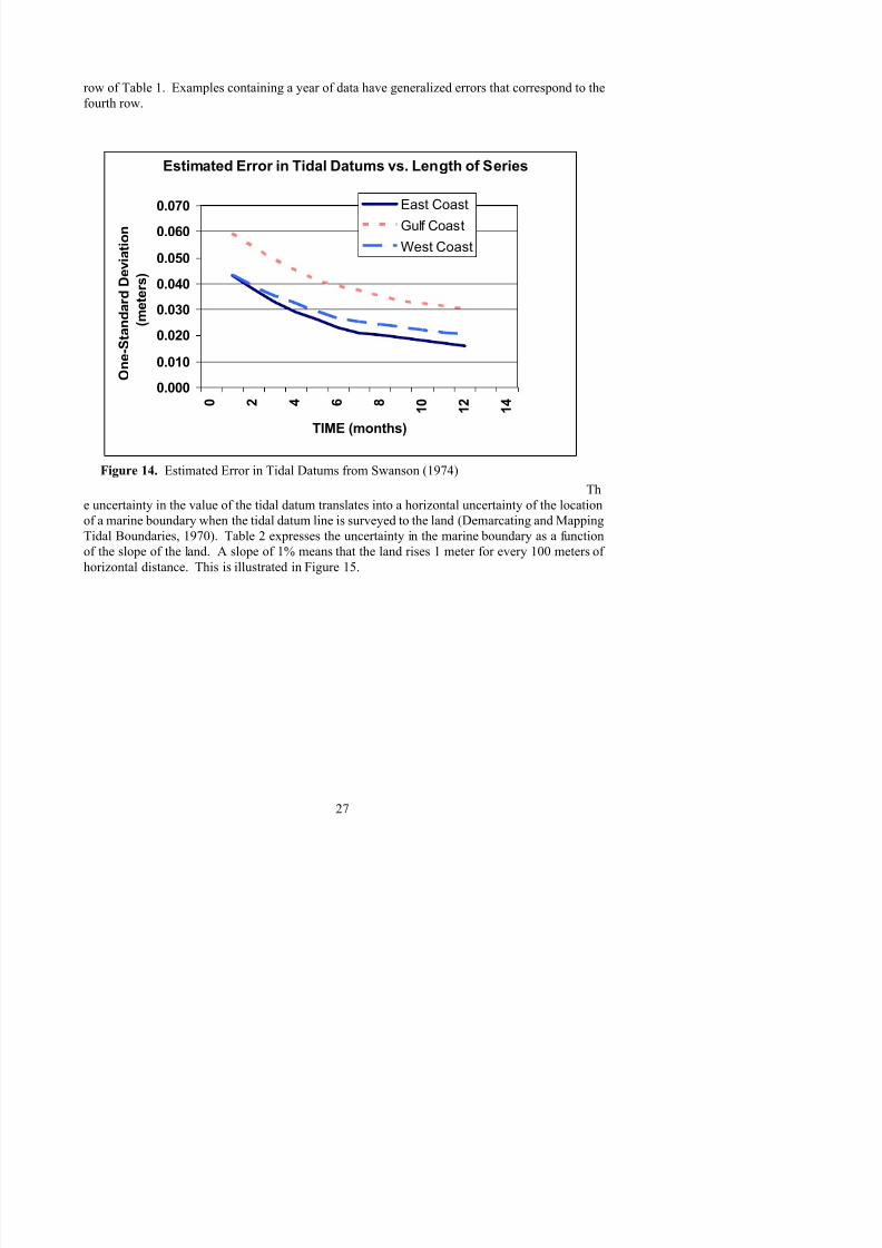
Figure 14. The estimated error in tidal datums from Swanson (1974) . . . . . . . . . . . . . . . . . . 27
Figure 15. Let x be the horizontal distance inland, and y the vertical rise of the land. By definition,tan(")=y/x. Likewise, the cotangent of ", denoted by cot("), is given by cot(") = x/y
. . . . . . . . . . . . . . . . . . . . . . . . . . . . . . . . . . . . . . . . . . . . . . . . . . . . . . . . . . . . . . . .
. . . . . . . . . . . . . . . . . . . . . . . . . . . . . . . . . . . . . . . . . . . . . . . . . . . . . . . . . . . . . . 28
Figure 16. NWLON station locations along the South Atlantic Bight . . . . . . . . . . . . . . . . . . 32
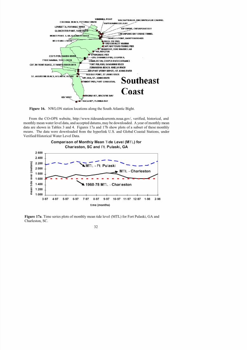
Figure 17a. Time series plots of monthly mean tide level (MTL) for Fort Pulaski, GA and
Charleston, SC. . . . . . . . . . . . . . . . . . . . . . . . . . . . . . . . . . . . . . . . . . . . . . . . . . . . . 32
Figure 17b. Time series plots of monthly mean range of tide (Mn) for Fort Pulaski, GA and
Charleston, SC. . . . . . . . . . . . . . . . . . . . . . . . . . . . . . . . . . . . . . . . . . . . . . . . . . . . . 33
Figure 18. A map showing NWLON stations in the Gulf of Mexico . . . . . . . . . . . . . . . . . . . 40
Figure 19a. Time series plots of monthly mean diurnal tide level (DTL) for Pensacola, FL andPanama City, FL. . . . . . . . . . . . . . . . . . . . . . . . . . . . . . . . . . . . . . . . . . . . . . . . . . . 41
Figure 19b. Time series plots of monthly mean diurnal range of tide (Gt) for Pensacola, FL and
Panama City, FL. . . . . . . . . . . . . . . . . . . . . . . . . . . . . . . . . . . . . . . . . . . . . . . . . . . 41
Figure 20. A map of California showing the locations of NWLON stations . . . . . . . . . . . . . . 47
Figure 21a. Time series plots of monthly mean tide level (MTL) for Alameda, CA and SanFrancisco, CA. . . . . . . . . . . . . . . . . . . . . . . . . . . . . . . . . . . . . . . . . . . . . . . . . . . . . 48
Figure 21b. Time series plots of monthly mean range of tide (Mn) for Alameda, CA and San
Francisco, CA. . . . . . . . . . . . . . . . . . . . . . . . . . . . . . . . . . . . . . . . . . . . . . . . . . . . . 48
8/6/2019 Computational Techniques for Tidal Datums Handbook
http://slidepdf.com/reader/full/computational-techniques-for-tidal-datums-handbook 9/113
LIST OF FIGURES (cont.)
pageFigure 23. The data returned from the CO-OPS database for Fort Pulaski, GA. Referring to Figure
31, the selection of “W3-Highs/Lows”, returns the data denoted by the diamond
symbols. Their values are also labeled. The rest of the curve is obtained by selecting
“W2-Hourly Heights”, and resubmitting the data request. . . . . . . . . . . . . . . . . . . 57
Figure 24. The data returned from the CO-OPS database for Charleston, SC . . . . . . . . . . . . 58
Figure 25. A graph of Charleston and Fort Pulaski data. The high water and low water valuesrequired for the tidal datum calculations are printed to illustrate the tide by tide
comparison. Refer to this graph when considering the organization of Table 26 below.
. . . . . . . . . . . . . . . . . . . . . . . . . . . . . . . . . . . . . . . . . . . . . . . . . . . . . . . . . . . . . . . . 59
Figure 26. A comparison of corresponding highs and lows for diurnal tides . . . . . . . . . . . . . 70
Figure 27. The water level time series for Alameda with the highs and lows plotted. The data are
referenced to station datum . . . . . . . . . . . . . . . . . . . . . . . . . . . . . . . . . . . . . . . . . . 78
Figure 28. The water level time series for San Francisco with the highs and lows plotted. The data
are referenced to station datum. . . . . . . . . . . . . . . . . . . . . . . . . . . . . . . . . . . . . . . . 78
Figure 29. A composite graph of Alameda and San Francisco. The time series at Alameda is
represented by the dashed curve. The data are referenced to station datum at each site.
. . . . . . . . . . . . . . . . . . . . . . . . . . . . . . . . . . . . . . . . . . . . . . . . . . . . . . . . . . . . . . . . 79
Figure 30. Comparison of data for a typical 7-day time period showing low waters cut-off at the
subordinate station . . . . . . . . . . . . . . . . . . . . . . . . . . . . . . . . . . . . . . . . . . . . . . . . . 83
8/6/2019 Computational Techniques for Tidal Datums Handbook
http://slidepdf.com/reader/full/computational-techniques-for-tidal-datums-handbook 10/113
LIST OF TABLES
pageTable 1. Generalized accuracy of tidal datums for East, Gulf, and West Coasts when determined
from short series of record and based on +/- sigma. From Swanson (1974) . . . . . . 26
Table 2. Error in position of marine boundary as a function of the slope of the land (12 month
series). . . . . . . . . . . . . . . . . . . . . . . . . . . . . . . . . . . . . . . . . . . . . . . . . . . . . . . . . . . . . 29
Table 3. NOS monthly mean water levels for Fort Pulaski, GA. These data are verified, monthly
mean values. STND refers to station datum, an arbitrary, vertical reference point at agiven location. . . . . . . . . . . . . . . . . . . . . . . . . . . . . . . . . . . . . . . . . . . . . . . . . . . . . . . 33
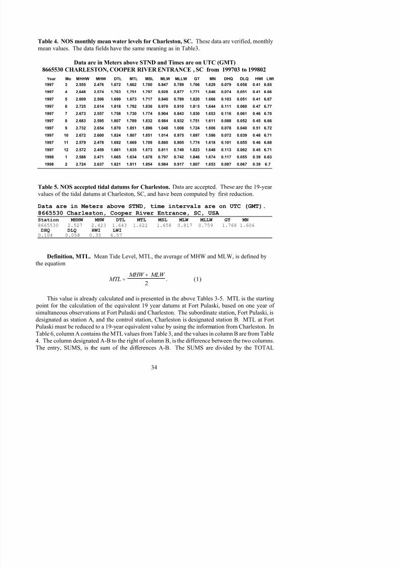
Table 4. NOS monthly mean water levels for Charleston, SC. These data are verified, monthly
mean values. The data fields have the same meaning as in Table 3. . . . . . . . . . . . . 34
Table 5. NOS tidal datums for Charleston. Data are accepted. These are the 19-year values of the
tidal datums at Charleston, SC, and have been computed by primary reduction. . . . 34
Table 6. Worksheet for calculating the corrected MTL for the subordinate station. The purpose
of this worksheet is to solve Eq. (2). . . . . . . . . . . . . . . . . . . . . . . . . . . . . . . . . . . . . 35
Table 7. Worksheet for calculating the corrected DTL for a subordinate station. This worksheet
solves Eq. 4. . . . . . . . . . . . . . . . . . . . . . . . . . . . . . . . . . . . . . . . . . . . . . . . . . . . . . . . . 36
Table 8. Worksheet for correcting the Mn at a subordinate station. This worksheet solves Eq. 6. . . . . . . . . . . . . . . . . . . . . . . . . . . . . . . . . . . . . . . . . . . . . . . . . . . . . . . . . . . . . . . . . . 37
Table 9. Worksheet for calculating the corrected Gt at a subordinate station. The purpose of this
worksheet is to solve Eq. 8. . . . . . . . . . . . . . . . . . . . . . . . . . . . . . . . . . . . . . . . . . . . . 38
Table 10. NOS monthly mean water levels for Panama City Beach, FL. . . . . . . . . . . . . . . . . 42
Table 11. NOS monthly mean water levels for Pensacola, FL. . . . . . . . . . . . . . . . . . . . . . . . . 42
Table 12. NOS accepted tidal datums for Pensacola. These are the 19-year, accepted, official values
of the tidal datums at Pensacola, FL, and have been computed by primary reduction. Note
that HWI -- Greenwich Mean High Water Interval in Hours, and LWI -- Greenwich Mean
Low Water Interval in Hours are not calculated for this station because the type of tide

8/6/2019 Computational Techniques for Tidal Datums Handbook
http://slidepdf.com/reader/full/computational-techniques-for-tidal-datums-handbook 11/113
LIST OF TABLES (cont.)
Table 14. Worksheet for calculating the corrected DTL for Panama City Beach. The purpose of thisTable is to solve Eq. 4 for Panama City Beach. . . . . . . . . . . . . . . . . . . . . . . . . . . . . 44
Table 15. Worksheet for correcting the Mn at a subordinate station . . . . . . . . . . . . . . . . . . . . 44
Table 16. Worksheet for calculating the corrected Gt at a subordinate station. . . . . . . . . . . . . 45
Table 17. NOS monthly mean water levels for Alameda, CA. The data are verified. . . . . . . 49
Table 18. NOS monthly mean water levels for San Francisco, CA. The data are verified. . . 49
Table 19. NOS tidal datums for San Francisco. Data are accepted. These are the 19-year values of
the tidal datums at San Francisco, CA, and have been computed by primary reduction.
The data are in meters above station datum. . . . . . . . . . . . . . . . . . . . . . . . . . . . . . . 50
Table 20. Worksheet for calculating the corrected MTL for Alameda. The purpose of this
worksheet is to solve Eq. (2). . . . . . . . . . . . . . . . . . . . . . . . . . . . . . . . . . . . . . . . . . . 50
Table 21. Worksheet for correcting the Mn at a subordinate station. The purpose of this worksheet
is to solve Eq. 6. . . . . . . . . . . . . . . . . . . . . . . . . . . . . . . . . . . . . . . . . . . . . . . . . . . . . 51
Table 22. Worksheet for calculating the corrected DHQ at a subordinate station. This worksheet
solves Eq. 14. . . . . . . . . . . . . . . . . . . . . . . . . . . . . . . . . . . . . . . . . . . . . . . . . . . . . . . . 52
Table 23. Worksheet for calculating the corrected DLQ at a subordinate station. This worksheet
solves Eq. 16. . . . . . . . . . . . . . . . . . . . . . . . . . . . . . . . . . . . . . . . . . . . . . . . . . . . . . . . 53
Table 24. NOS High and Low Waters for 8670870 Fort Pulaski, Savannah River, GA, USA from
19960304 to 19960308. Data are verified. Data are in meters above Station Datum
(STND). Times are on UTC (GMT). The fields in the table have the following meanings.
Station--Unique seven character identifier for the station. Date Time--Date and time the
data were collected by the DCP. WL_Value--Water level height. Type --Designation of Water level height. LL = lower low water, L = low water, H = High water, HH Higher
High water. Infer--A flag that indicates that the water level value has been inferred.
Limit--A flag that when set to 1 indicates that either the maximum or minimum expected
water level height limit was exceeded. . . . . . . . . . . . . . . . . . . . . . . . . . . . . . . . . . . . 56
8/6/2019 Computational Techniques for Tidal Datums Handbook
http://slidepdf.com/reader/full/computational-techniques-for-tidal-datums-handbook 12/113
LIST OF TABLES (cont.)
Table 26. Comparison of simultaneous observations for 96-3-4 TO 96-3-8. Datums computed for the 1960-1978 tidal epoch. (A) designates the subordinate station, 8670870, Fort Pulaski,
Savannah River, GA. (B) designates the control or, standard station 8665530,
Charleston, Cooper River Entrance, SC. . . . . . . . . . . . . . . . . . . . . . . . . . . . . . . . . . . 60
Table 27. Calculation of the mean time differences between the subordinate and control stations.
The means computed below are entered into Equations 48 and 49 to estimate the
Greenwich lunitidal intervals at the subordinate station. The times entered below are in
GMT. . . . . . . . . . . . . . . . . . . . . . . . . . . . . . . . . . . . . . . . . . . . . . . . . . . . . . . . . . . . . 67
Table 28. NOS high and low waters for 8729210 Panama City Beach, FL, USA from 1996-03-10
to 1996-03-16. Data are verified. Data are in meters above STND. Times are on UTC
(GMT). . . . . . . . . . . . . . . . . . . . . . . . . . . . . . . . . . . . . . . . . . . . . . . . . . . . . . . . . . . . 69
Table 29. NOS high and low waters for 8729840 Pensacola, Pensacola Bay, FL, USA from 1996-
03-10 to 1996-03-16. Data are verified. Data are in meters above STND. Times are on
UTC (GMT). . . . . . . . . . . . . . . . . . . . . . . . . . . . . . . . . . . . . . . . . . . . . . . . . . . . . . . . 69
Table 30. Worksheet for computing a tide by tide comparison of high and low waters, diurnal
example. Refer to Figure 31 to see how the high and low waters are matched. . . . 70
Table 31. Computation of the mean time differences between Panama City Beach and Pensacola,
FL.. . . . . . . . . . . . . . . . . . . . . . . . . . . . . . . . . . . . . . . . . . . . . . . . . . . . . . . . . . . . . . . 74
Table 32. NOS high and low waters for 9414750 Alameda, San Francisco Bay, CA, USA from
1997-03-01 to 1997-03-07. Data are verified. Data are in meters above STND. Times
are on UTC (GMT). . . . . . . . . . . . . . . . . . . . . . . . . . . . . . . . . . . . . . . . . . . . . . . . . . . 75
Table 33. NOS high and low waters for 9414290 San Francisco, San Francisco Bay, CA, USA from
1997-03-01 to 1997-03-07. Data are verified. Data are in meters above STND. Times
are on UTC (GMT). . . . . . . . . . . . . . . . . . . . . . . . . . . . . . . . . . . . . . . . . . . . . . . . . . . 76
Table 34. Worksheet for calculating a tide by tide analysis for a mixed tide case. . . . . . . . . . 77
Table 35. Computation of the mean time differences between Alameda and San Francisco, CA
. . . . . . . . . . . . . . . . . . . . . . . . . . . . . . . . . . . . . . . . . . . . . . . . . . . . . . . . . . . . . . . . . . 82
8/6/2019 Computational Techniques for Tidal Datums Handbook
http://slidepdf.com/reader/full/computational-techniques-for-tidal-datums-handbook 13/113
LIST OF ACRONYMS
CO-OPS Center for Operational Oceanographic Products and ServicesDQA Data Quality Assurance
DHQ Mean Diurnal High Water Inequality
DLQ Mean Diurnal Low Water Inequality
DTL Diurnal Tide Level
GMT Greenwich Mean Time
GPS Global Positioning System
Gt Great Tropic Range
IGLD 85 International Great Lakes Datum of 1985HHW Higher High Water
HLW Higher Low Water
HWI High Water Lunitidal Interval
HWL Highest Water Level
LHW Lower High Water
LLW Lower Low Water
LW Low Water
LWI Low Water Lunitidal Interval
LWL Lowest Water Level
MHW Mean High Water
MHHW Mean Higher High Water
MLW Mean Low Water
MLLW Mean Lower Low Water
Mn Mean Range of Tide
MSL Mean Sea LevelMTL Mean Tide Level
NAVD 88 North American Vertical Datum of 1988
NGWLMS Next Generation Water Level Measurement System
NGVD 29 National Geodetic Vertical Datum of 1929
NIST National Institutes of Standards and Technology
NOAA National Oceanic and Atmospheric Administration
NOS National Ocean Service
NTBMS National Tidal Benchmark System NTDE National Tidal Datum Epoch
NWLON National Water Level Observation Network
NWLP National Water Level Program
PBM Primary Bench Mark
QA Quality Assurance

8/6/2019 Computational Techniques for Tidal Datums Handbook
http://slidepdf.com/reader/full/computational-techniques-for-tidal-datums-handbook 14/113
8/6/2019 Computational Techniques for Tidal Datums Handbook
http://slidepdf.com/reader/full/computational-techniques-for-tidal-datums-handbook 15/113
1. INTRODUCTION
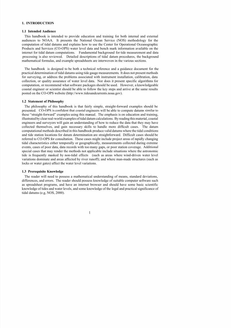
1.1 Intended AudienceThis handbook is intended to provide education and training for both internal and external
audiences to NOAA. It presents the National Ocean Service (NOS) methodology for the
computation of tidal datums and explains how to use the Center for Operational Oceanographic
Products and Services (CO-OPS) water level data and bench mark information available on the
internet for tidal datum computations. Fundamental background for tide measurement and data
processing is also reviewed. Detailed descriptions of tidal datum procedures, the background
mathematical formulas, and example spreadsheets are interwoven in the various sections.
The handbook is designed to be both a technical reference and a guidance document for the
practical determination of tidal datums using tide gauge measurements. It does not present methods
for surveying, or address the problems associated with instrument installation, calibration, data
collection, or quality assurance of water level data. Nor does it present specific algorithms for
computation, or recommend what software packages should be used. However, a knowledgeable
coastal engineer or scientist should be able to follow the key steps and arrive at the same results
posted on the CO-OPS website (http://www.tidesandcurrents.noaa.gov).
1.2 Statement of Philosophy
The philosophy of this handbook is that fairly simple, straight-forward examples should be
presented. CO-OPS is confident that coastal engineers will be able to compute datums similar to
these “straight-forward” examples using this manual. The emphasis is on education and training,
illustrated by clear real-world examples of tidal datum calculations. By reading this material, coastal
engineers and surveyors will gain an understanding of how to reduce the data that they may have
collected themselves, and gain necessary skills to handle more difficult cases. The datumcomputational methods described in this handbook produce valid datums where the tidal conditions
and tide station locations for datum determination are straightforward. Difficult cases should be
referred to CO-OPS for consultation. These cases might include project areas of rapidly changing
tidal characteristics either temporally or geographically, measurements collected during extreme
events, cases of poor data, data records with too many gaps, or poor station coverage. Additional
special cases that may render the methods not applicable include situations where the astronomic
tide is frequently masked by non-tidal effects (such as areas where wind-driven water level
variations dominate and areas affected by river runoff); and where man-made structures (such as
locks or water gates) affect the water level variations.
1.3 Prerequisite Knowledge
The reader will need to possess a mathematical understanding of means, standard deviations,

8/6/2019 Computational Techniques for Tidal Datums Handbook
http://slidepdf.com/reader/full/computational-techniques-for-tidal-datums-handbook 16/113

8/6/2019 Computational Techniques for Tidal Datums Handbook
http://slidepdf.com/reader/full/computational-techniques-for-tidal-datums-handbook 17/113
8/6/2019 Computational Techniques for Tidal Datums Handbook
http://slidepdf.com/reader/full/computational-techniques-for-tidal-datums-handbook 18/113
Figure 3 shows the gradual spatial transitions from mixed to diurnal to mixed and back to diurnal
in the Gulf of Mexico. It is important to know the location of these transition zones because they
limit how far the datum computation procedures described in this document can be appliedsuccessfully.
8/6/2019 Computational Techniques for Tidal Datums Handbook
http://slidepdf.com/reader/full/computational-techniques-for-tidal-datums-handbook 19/113
COMPARISON OF TIDE TYPES OVER ONE CALENDAR MONTH
-0.500
0.500
1.500
2.500
3.500
4.500
5.500
6.500
7.500
8.500
01-01-02 01-06-02 01-11-02 01-16-02 01-21-02 01-26-02 01-31-02
Time (hours)
E l e v a t i o n
( m e t e r s )
Semidiurnal - Fort Pulaski, GA
Mixed - San Francisco, CA
Diurnal - Pensacola, FL
Figure 2. Comparison of types of tide over one-calendar month.
8/6/2019 Computational Techniques for Tidal Datums Handbook
http://slidepdf.com/reader/full/computational-techniques-for-tidal-datums-handbook 20/113
Figure 4. An illustration of the effect of the regression of the moon’s nodes on the water levels atPuget Sound, WA. The heavy black curve is the annual mean range, or the difference in height
between mean high water and mean low water. The time elapsed between trough to trough, or
peak to peak, is the period of oscillation of the regression, and is about 18.6 years. The more
rapidly varying curve is the monthly mean range. Changes in the monthly mean range are due to
rapidly changing meteorological and oceanographic conditions.
There is a variation in the path of the moon about the earth that has a period of about 18.6 years, and
is called the regression of the moon’s nodes. The regression of the nodes introduces an important
variation into the amplitude of the monthly and annual mean range of the tide, as may be seen inFigure 4. It is the regression of the moon’s nodes which forms the basis of the definition of the
National Tidal Datum Epoch (NTDE). Because the variability of the monthly mean range is larger
than the regression of the nodes, the National Tidal Datum Epoch is defined as an even 19 year
period so as not to bias the estimate of the tidal datum.
8/6/2019 Computational Techniques for Tidal Datums Handbook
http://slidepdf.com/reader/full/computational-techniques-for-tidal-datums-handbook 21/113
Greenwich interval local interval= + 0069. L
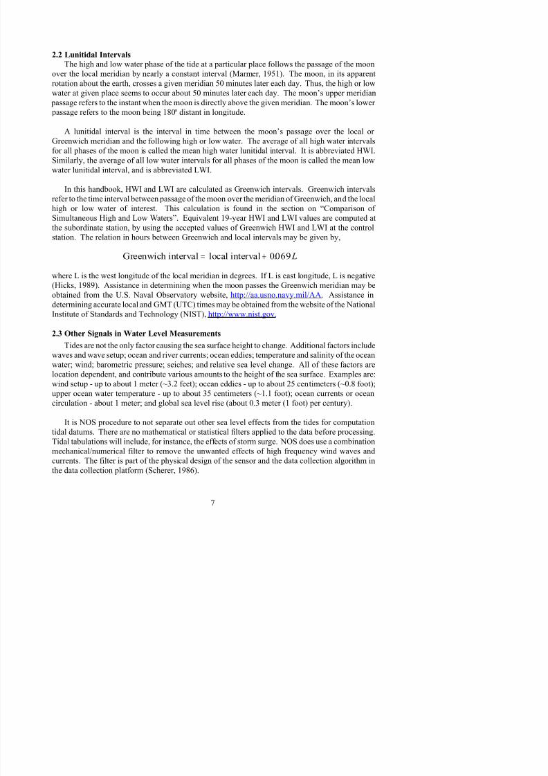
2.2 Lunitidal Intervals
The high and low water phase of the tide at a particular place follows the passage of the moon
over the local meridian by nearly a constant interval (Marmer, 1951). The moon, in its apparentrotation about the earth, crosses a given meridian 50 minutes later each day. Thus, the high or low
water at given place seems to occur about 50 minutes later each day. The moon’s upper meridian
passage refers to the instant when the moon is directly above the given meridian. The moon’s lower
passage refers to the moon being 180o distant in longitude.
A lunitidal interval is the interval in time between the moon’s passage over the local or
Greenwich meridian and the following high or low water. The average of all high water intervals
for all phases of the moon is called the mean high water lunitidal interval. It is abbreviated HWI.Similarly, the average of all low water intervals for all phases of the moon is called the mean low
water lunitidal interval, and is abbreviated LWI.
In this handbook, HWI and LWI are calculated as Greenwich intervals. Greenwich intervals
refer to the time interval between passage of the moon over the meridian of Greenwich, and the local
high or low water of interest. This calculation is found in the section on “Comparison of
Simultaneous High and Low Waters”. Equivalent 19-year HWI and LWI values are computed at
the subordinate station, by using the accepted values of Greenwich HWI and LWI at the controlstation. The relation in hours between Greenwich and local intervals may be given by,
where L is the west longitude of the local meridian in degrees. If L is east longitude, L is negative
(Hicks, 1989). Assistance in determining when the moon passes the Greenwich meridian may be
obtained from the U.S. Naval Observatory website, http://aa.usno.navy.mil/AA. Assistance indetermining accurate local and GMT (UTC) times may be obtained from the website of the National
Institute of Standards and Technology (NIST), http://www.nist.gov.
2.3 Other Signals in Water Level Measurements
Tides are not the only factor causing the sea surface height to change. Additional factors include
waves and wave setup; ocean and river currents; ocean eddies; temperature and salinity of the ocean
water; wind; barometric pressure; seiches; and relative sea level change. All of these factors are
location dependent, and contribute various amounts to the height of the sea surface. Examples are:wind setup - up to about 1 meter (~3.2 feet); ocean eddies - up to about 25 centimeters (~0.8 foot);
upper ocean water temperature - up to about 35 centimeters (~1.1 foot); ocean currents or ocean
circulation - about 1 meter; and global sea level rise (about 0.3 meter (1 foot) per century).
It i NOS d t t t t th l l ff t f th tid f t ti

8/6/2019 Computational Techniques for Tidal Datums Handbook
http://slidepdf.com/reader/full/computational-techniques-for-tidal-datums-handbook 22/113
2.4 Tide Station Networks
The NOS National Water Level Program (NWLP) provides unique water level and ancillary data
sets and information to users in support of a wide variety of critical activities. A priority of the NWLP is to provide the basic data for the vertical, tidal datum control for the nation. For instance,
these data specifically support NOAA’s Nautical Charting and safe navigation programs. The
instrumentation of the NWLP consists of water level stations in the National Water Level
Observation Network (NWLON), and any short-term stations operating for special projects such as
hydrographic surveys, photogrammetry, and United States Army Corps of Engineers (USACE)
dredging activities. The NWLON (Figure 5) is composed (as of year 2000) of approximately 175
long term stations distributed around the country and the world. The applications supported by the
NWLON include: nautical charting, hydrography, remote sensing for shoreline, boundarydetermination, navigation, channel dredging and harbor improvements, tsunami and storm surge
warnings, tide predictions, environmental monitoring and habitat restoration, climate and global
change, international lake level regulation, international treaty compliance, and international
boundary determination.
Except for water level stations in the Great Lakes, most of the stations in the NWLON are in
coastal areas that come under the influence of the tide to a significant degree and are referred to as
control tide stations. These stations have accepted tidal datums computed over the NDTE or at least
over a several year period from which equivalent NTDE accepted values have been computed. This
network provides direct datum control for a nearby areas and control for short-term stations for a
larger geographic area. The extent of datum control depends upon the complexity of the coastal
zone in terms of changes in tidal characteristics, localized effects of river runoff and wind, and
differences in long-term sea level trends.
The NWLON is designed to provide a nationwide fundamental tidal datum control network.Most applications require tidal datum information at a higher resolution than that provided by the
NWLON network spacing. Depending on the application, networks of shorter-term stations are
established.
Control tide stations are generally those which have been operated for 19 or more years, are
expected to continuously operate in the future, and are used to obtain a continuous record of the
water levels in a locality. Control tide stations are sited to provide datum control for national
applications, and located in as many places as needed for datum control. As the records from sucha station constitute basic water level data for present and future use, during the installation and
maintenance of the station, the aim is to obtain the highest degree of reliability and precision that
is practical. The essential equipment of a control tide station includes an automatic water level
sensor, protective well, shelter, back-up water level sensor, a system of bench marks, and possibly
ill h i l i t t

8/6/2019 Computational Techniques for Tidal Datums Handbook
http://slidepdf.com/reader/full/computational-techniques-for-tidal-datums-handbook 23/113
Figure 5. Locations of U.S. NWLON water level stations.
but when reduced by comparison with simultaneous observations at a suitable control tide station
very satisfactory results may be obtained. Secondary tide stations may also provide data for the
reduction of soundings in connection with hydrographic surveys.
Tertiary water level stations are those which are operated for more than a month but less than1 year. Short-term water level measurement stations (secondary and tertiary) may have their data
reduced to equivalent 19-year tidal datums through mathematical simultaneous comparison with a
nearby control station. Short-term data, often at several locations, are collected routinely to support
hydrographic surveying. In the Great Lakes, seasonal data are compared to simultaneous
observations from adjacent stations for datum determination in harbors
8/6/2019 Computational Techniques for Tidal Datums Handbook
http://slidepdf.com/reader/full/computational-techniques-for-tidal-datums-handbook 24/113
include coverage of critical navigation areas and transitional zones, historical sites, proximity to the
geodetic network, and the availability of existing structures, such as piers suitable for the location
of the scientific equipment.
Site reconnaissance is performed prior to the installation of a new station. Field site visits are
made to aid in the design, make measurements, and render technical drawings; to recover bench
marks, or plan for new bench marks; and to obtain permission, permits, agreements, etc. The field
parties take into consideration the requirements for the installation and protection of the instruments.
The most important considerations are the presence of a suitable structure, the necessary benchmark
locations, adequate water depth, special materials that might be needed to prevent marine fouling
and corrosion, availability of telephone and electrical service, site security, and lightning protection.
There are numerous types of tide gauges and sensors that can be used for tidal datum
computation purposes. NOS specifications for tide station installations and data processing and
reduction for NOS hydrographic surveys are found in NOS Hydrographic Survey Specifications and
Deliverables (NOS,2003). International references include the Manual on Sea level Measurement
and Interpretation (IOC, 2000). The latest update on NOS water level measurement systems and
capabilities are found in Mero, 1998. For tidal datum applications, it is important for gauge sensors
to be carefully calibrated with either frequent calibration checks or cycled swaps of calibratedsensors for long-term installations. The sensor “zero” must be precisely related to either a tide staff
and/or the bench marks through staff/gauge comparisons or direct leveling between the sensor and
the bench marks. Vertical stability of the sensor “zero”, both physically and internally, must be
monitored and any movement taken into account in the data reduction and datum computation.
2.5 Bench marks and Differential Leveling
A network of bench marks is an integral part of every water level measurement station. A benchmark is a fixed physical object or mark (sometimes referred to as a monument) used as a reference
for a vertical datum. For example, a tidal bench mark is a mark near a tide station to which the tidal
datums are referenced. Since gauge measurements are referenced to the bench marks, it follows that
the overall quality of the datums is partly dependent on both the quality of the bench mark
installation and the quality of the leveling between the bench marks and the gauge.
Bench marks have site selection considerations much like the tide stations they support. The
first consideration is longevity; bench marks are sited to minimize susceptibility to damage or destruction. Bench marks are sited to ease future recovery (locating and leveling to the mark) and
to ensure accessibility (open, overhead clearance). Bench marks must also be placed in the most
stable structure for the locality. Preference should be given to disks set in bedrock, in large man
made structures with deep foundations, or installation of stainless steel rods driven to substantial
i t Si b h k l bl t t l di t b h l i d il
8/6/2019 Computational Techniques for Tidal Datums Handbook
http://slidepdf.com/reader/full/computational-techniques-for-tidal-datums-handbook 25/113
8/6/2019 Computational Techniques for Tidal Datums Handbook
http://slidepdf.com/reader/full/computational-techniques-for-tidal-datums-handbook 26/113
station. Five bench marks are installed at secondary and tertiary stations. At least three bench
marks are installed at short term (less than 30 days) stations.
Bench marks are leveled whenever a new tide station is established, or when data collection is
discontinued at a tide station. Bench marks are also leveled before and after maintenance is
performed at a station, and at least annually to perform stability checks. In addition, whenever new
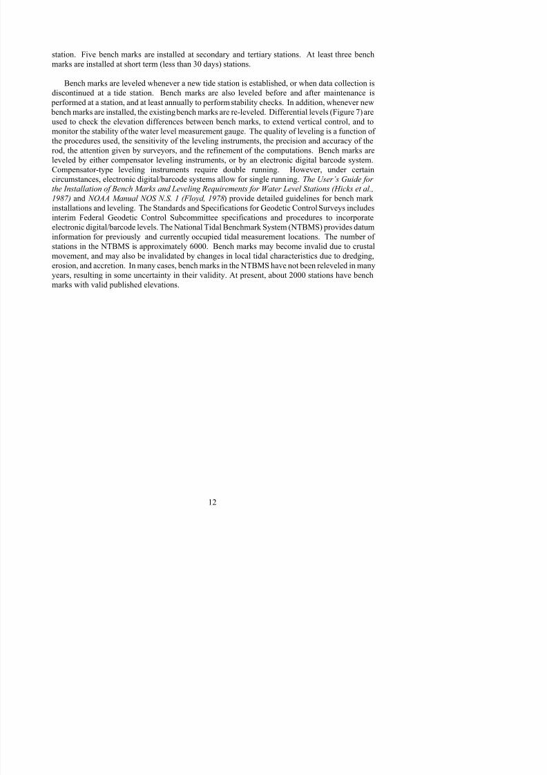
bench marks are installed, the existing bench marks are re-leveled. Differential levels (Figure 7) are
used to check the elevation differences between bench marks, to extend vertical control, and to
monitor the stability of the water level measurement gauge. The quality of leveling is a function of
the procedures used, the sensitivity of the leveling instruments, the precision and accuracy of the
rod, the attention given by surveyors, and the refinement of the computations. Bench marks areleveled by either compensator leveling instruments, or by an electronic digital barcode system.
Compensator-type leveling instruments require double running. However, under certain
circumstances, electronic digital/barcode systems allow for single running. The User’s Guide for
the Installation of Bench Marks and Leveling Requirements for Water Level Stations (Hicks et al.,
1987) and NOAA Manual NOS N.S. 1 (Floyd, 1978) provide detailed guidelines for bench mark
installations and leveling. The Standards and Specifications for Geodetic Control Surveys includes
interim Federal Geodetic Control Subcommittee specifications and procedures to incorporate
electronic digital/barcode levels. The National Tidal Benchmark System (NTBMS) provides datuminformation for previously and currently occupied tidal measurement locations. The number of
stations in the NTBMS is approximately 6000. Bench marks may become invalid due to crustal
movement, and may also be invalidated by changes in local tidal characteristics due to dredging,
erosion, and accretion. In many cases, bench marks in the NTBMS have not been releveled in many
years, resulting in some uncertainty in their validity. At present, about 2000 stations have bench
marks with valid published elevations.
8/6/2019 Computational Techniques for Tidal Datums Handbook
http://slidepdf.com/reader/full/computational-techniques-for-tidal-datums-handbook 27/113
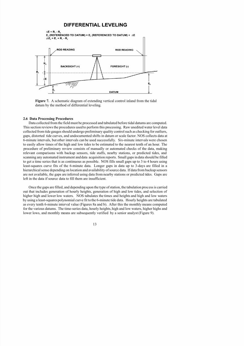
Figure 7. A schematic diagram of extending vertical control inland from the tidaldatum by the method of differential leveling.
2.6 Data Processing Procedures
Data collected from the field must be processed and tabulated before tidal datums are computed.
This section reviews the procedures used to perform this processing. Raw unedited water level data
collected from tide gauges should undergo preliminary quality control such as checking for outliers,
gaps, distorted tide curves, and undocumented shifts in datum or scale factor. NOS collects data at
6-minute intervals, but other intervals can be used successfully. Six-minute intervals were chosen
to easily allow times of the high and low tides to be estimated to the nearest tenth of an hour. The
procedure of preliminary review consists of manually or automated checks of the data, making
relevant comparisons with backup sensors, tide staffs, nearby stations, or predicted tides, and
scanning any automated instrument and data acquisition reports. Small gaps in data should be filled
to get a time series that is as continuous as possible. NOS fills small gaps up to 3 to 4 hours using
least-squares curve fits of the 6-minute data. Longer gaps in data up to 3-days are filled in ahierarchical sense depending on location and availability of source data. If data from backup sensors
are not available, the gaps are inferred using data from nearby stations or predicted tides. Gaps are
left in the data if source data to fill them are insufficient.
Once the gaps are filled and depending upon the type of station the tabulation process is carried

8/6/2019 Computational Techniques for Tidal Datums Handbook
http://slidepdf.com/reader/full/computational-techniques-for-tidal-datums-handbook 28/113
8454049 QUONSET POINT RI - Six Minute - Water Level : October 2002
6.000
6.500
7.000
7.500
8.000
8.500
9.000
10-01-02 00:00 10-06-02 00:00 10-11-02 00:00 10-16-02 00:00 10-21-02 00:00 10-26-02 00:00 10-31-02 00:00
E l e v a t i o n R e l a t i v e t o S t a t i o n D a
t u m
( m e t e r s )
8/6/2019 Computational Techniques for Tidal Datums Handbook
http://slidepdf.com/reader/full/computational-techniques-for-tidal-datums-handbook 29/113
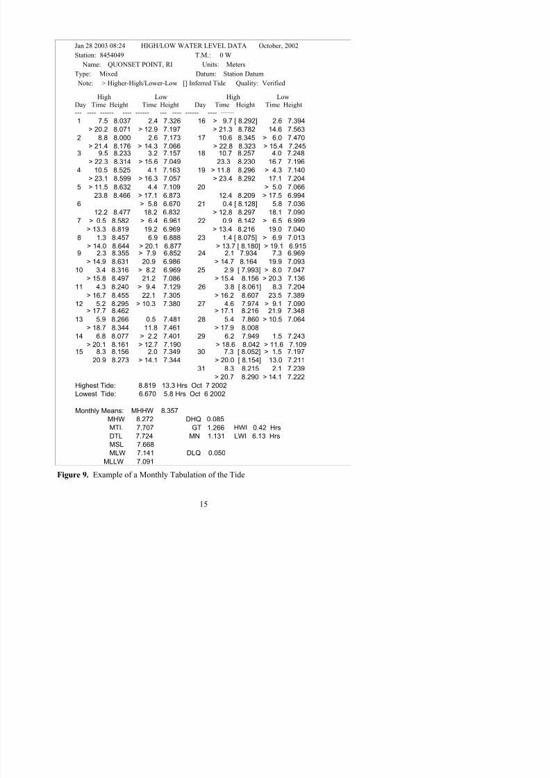
Jan 28 2003 08:24 HIGH/LOW WATER LEVEL DATA October, 2002
Station: 8454049 T.M.: 0 W
Name: QUONSET POINT, RI Units: Meters
Type: Mixed Datum: Station Datum
Note: > Higher-High/Lower-Low [] Inferred Tide Quality: Verified
High Low High LowDay Time Height Time Height Day Time Height Time Height--- ---- ------ ---- ------ --- ---- ------ ---- ------
1 7.5 8.037 2.4 7.326 16 > 9.7 [ 8.292] 2.6 7.394
> 20.2 8.071 > 12.9 7.197 > 21.3 8.782 14.6 7.563
2 8.8 8.000 2.6 7.173 17 10.6 8.345 > 6.0 7.470
> 21.4 8.176 > 14.3 7.066 > 22.8 8.323 > 15.4 7.245
3 9.5 8.233 3.2 7.157 18 10.7 8.257 4.0 7.248> 22.3 8.314 > 15.6 7.049 23.3 8.230 16.7 7.196
4 10.5 8.525 4.1 7.163 19 > 11.8 8.296 > 4.3 7.140
> 23.1 8.599 > 16.3 7.057 > 23.4 8.292 17.1 7.204
5 > 11.5 8.632 4.4 7.109 20 > 5.0 7.066
23.8 8.466 > 17.1 6.873 12.4 8.209 > 17.5 6.994
6 > 5.8 6.670 21 0.4 [ 8.128] 5.8 7.036
12.2 8.477 18.2 6.832 > 12.8 8.297 18.1 7.090
7 > 0.5 8.582 > 6.4 6.961 22 0.9 8.142 > 6.5 6.999
> 13.3 8.819 19.2 6.969 > 13.4 8.216 19.0 7.0408 1.3 8.457 6.9 6.888 23 1.4 [ 8.075] > 6.9 7.013
> 14.0 8.644 > 20.1 6.877 > 13.7 [ 8.180] > 19.1 6.9159 2.3 8.355 > 7.9 6.852 24 2.1 7.934 7.3 6.969
> 14.9 8.631 20.9 6.986 > 14.7 8.164 19.9 7.093
10 3.4 8.316 > 8.2 6.969 25 2.9 [ 7.993] > 8.0 7.047
> 15.8 8.497 21.2 7.086 > 15.4 8.156 > 20.3 7.136
11 4.3 8.240 > 9.4 7.129 26 3.8 [ 8.061] 8.3 7.204
> 16.7 8.455 22.1 7.305 > 16.2 8.607 23.5 7.389
12 5.2 8.295 > 10.3 7.380 27 4.6 7.974 > 9.1 7.090> 17.7 8.462 > 17.1 8.216 21.9 7.348
13 5.9 8.266 0.5 7.481 28 5.4 7.860 > 10.5 7.064
> 18.7 8.344 11.8 7.461 > 17.9 8.008
14 6.8 8.077 > 2.2 7.401 29 6.2 7.949 1.5 7.243
> 20.1 8.161 > 12.7 7.190 > 18.6 8.042 > 11.6 7.10915 8.3 8.156 2.0 7.349 30 7.3 [ 8.052] > 1.5 7.197
20.9 8.273 > 14.1 7.344 > 20.0 [ 8.154] 13.0 7.211
31 8.3 8.215 2.1 7.239
> 20.7 8.290 > 14.1 7.222Highest Tide: 8.819 13.3 Hrs Oct 7 2002
Lowest Tide: 6.670 5.8 Hrs Oct 6 2002
Monthly Means: MHHW 8.357
MHW 8.272 DHQ 0.085
8/6/2019 Computational Techniques for Tidal Datums Handbook
http://slidepdf.com/reader/full/computational-techniques-for-tidal-datums-handbook 30/113
2.7 The National Tidal Datum Epoch
As mentioned in section 2.1, a specific nineteen year period designated as a National Tidal
datum Epoch (NTDE) is used to compute tidal datums because it is the closest full year to the 18.6-year nodal cycle, the period required for the regression of the moon’s nodes to complete a circuit
of 360/ of longitude (Schureman, 1941). The NTDE is used as the fixed period of time for the
determination tidal datums because it includes all significant tidal periods, is long enough to average
out the local meteorological effects on sea level, and by specifying the NTDE, a uniform approach
is applied to the tidal datums for all stations.
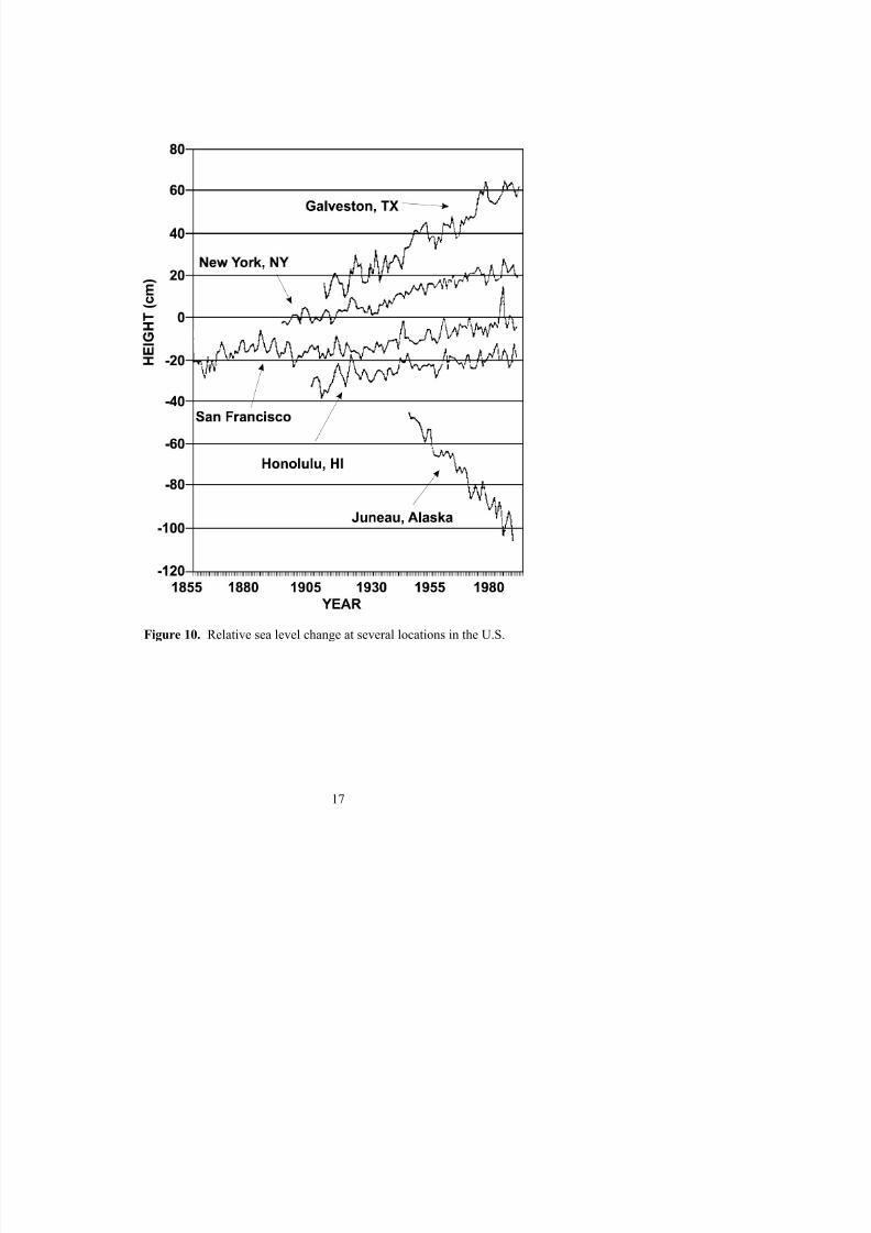
The relative secular sea level change, as well as the variability of the change by geographic
region, is readily seen (Figure 10) where the yearly mean sea level is plotted against time. For datum computation, the National Tidal Datum Epoch is used as the fixed period of time for the
determination of tidal datums because it includes all significant tidal periods, is long enough to
average out the local meteorological effects on sea level, and by specifying the NTDE, uniformity
is applied to all the tidal datums. However, because of relative sea level change, as the years pass,
tidal datums become out of date for navigational purposes and for other applications. Thus, a new
NTDE must be considered periodically (Hicks, 1981). The policy of NOS is to consider a new tidal
datum epoch every 25 years to appropriately update the tidal datums to account for the global sea
level change and long-term vertical adjustment of the local landmass (e.g., due to subsidence or
glacial rebound)(Gill et al, 1998). Figure 11 shows the effect of sea level rise on the elevation of
MTL over various NDTE periods. NOS will be updating from the 1960-78 NTDE to a 1983-2001
NTDE in 2003. Estimated relative sea level trends compiled from observations at U.S. tide stations
are found in Zervas (2000).
8/6/2019 Computational Techniques for Tidal Datums Handbook
http://slidepdf.com/reader/full/computational-techniques-for-tidal-datums-handbook 31/113
Figure 10. Relative sea level change at several locations in the U.S.

8/6/2019 Computational Techniques for Tidal Datums Handbook
http://slidepdf.com/reader/full/computational-techniques-for-tidal-datums-handbook 32/113
San Francisco, CA - Variations in MTL Across National
Tidal Datum Epochs
2.200
2.300
2.400
2.500
2.600
2.700
2.800
2.900
3.000
3.100
3.200
1 - 0 0
1 - 0 4
1 - 0 8
1 - 1 2
1 - 1 6
1 - 2 0
1 - 2 4
1 - 2 8
1 - 3 2
1 - 3 6
1 - 4 0
1 - 4 4
1 - 4 8
1 - 5 2
1 - 5 6
1 - 6 0
1 - 6 4
1 - 6 8
1 - 7 2
1 - 7 6
1 - 8 0
1 - 8 4
1 - 8 8
1 - 9 2
1 - 9 6
time (months)
m e a n t i d e l e v e l ( m e t e r s )
1941-59 MTL :2.700m 1960-78 MTL: 2.728m
Figure 11. Illustration of the long term changes in sea level causing the need to update
tidal datums such as mean tide level (MTL). The graph shows the annual values of mean
tide level with horizontal lines drawn to show the 19-year MTL values for the 1941-59 and
1960-78 NTDE.

8/6/2019 Computational Techniques for Tidal Datums Handbook
http://slidepdf.com/reader/full/computational-techniques-for-tidal-datums-handbook 33/113
3. GENERAL TIDAL DATUM COMPUTATION PROCEDURES
3.1 Datum Computation Procedures Overview
A vertical datum is termed a tidal datum when it is defined by a certain phase of the tide. Tidal
datums are local datums and should not be extended into areas which have differing hydrographic
characteristics without substantiating measurements. In order that they may be recovered when
needed, such datums are referenced to fixed points known as bench marks.
1. Make Observations - Tidal datums are computed from continuous water level observations
over specified lengths of time. Observations are made at specific locations called tide stations. Each
tide station consists of a water level gauge or sensor(s), a data collection platform or data logger anddata transmission system, and a set of tidal bench marks established in the vicinity of the tide station.
NOS collects water level data at 6-minute intervals.
2. Tabulate the Tide - Once the 6-minute interval data are quality controlled and any small gaps
filled, the data are processed by tabulating the high and low tides and hourly heights for each day.
Tidal parameters from these daily tabulations of the tide are then reduced to mean values, typically
on a calendar month basis for longer period records or over a few days or weeks for shorter-term
records.
3. Compute Tidal Datums - First reduction tidal datums are determined directly by averaging
values of the tidal parameters over a 19-year NDTE. Equivalent NDTE tidal datums are computed
from tide stations operating for shorter time periods through comparison of simultaneous data
between the short-term station and a long term station.
4. Compute Bench Mark Elevations - Once the tidal datums are computed from thetabulations, the elevations are referenced to the bench marks established on the land using the
elevation differences established by differential leveling between the tide gauge sensor “zero” and
the bench marks during the station operation. The bench mark elevations and descriptions are
disseminated by NOS through a station specific published bench mark sheet. Connections between
tidal datum elevations and geodetic elevations are obtained after leveling between tidal bench marks
and geodetic network bench marks. Traditionally, this has been accomplished using differential
leveling, however GPS surveying techniques can also be used (NGS, 1997).
A primary determination of any tidal datum is based directly on the average of observations over
a 19 year period. For example, a primary determination of Mean High Water is based directly on the
average of the high waters over a 19 year period. Tidal datums must be specified with regard to the
NTDE. Although many tidal datums are discussed in this report, the principal tidal datums include
M Hi h Hi h W t (MHHW) M Hi h W t (MHW) M S L l (MSL) M L

8/6/2019 Computational Techniques for Tidal Datums Handbook
http://slidepdf.com/reader/full/computational-techniques-for-tidal-datums-handbook 34/113
8/6/2019 Computational Techniques for Tidal Datums Handbook
http://slidepdf.com/reader/full/computational-techniques-for-tidal-datums-handbook 35/113
adopted as a standard geodetic reference for heights and was derived from a general adjustment of
the first order leveling nets of the US and Canada, in which MSL was held fixed as observed at 26
stations in the US and Canada. Numerous adjustments have been made to these leveling networks
since originally established in 1929. The North American Vertical Datum of 1988 (NAVD 88)
involved a simultaneous least-squares, minimum constraint adjustment of the Canadian-Mexican-US
leveling observations. Local MSL was held fixed at Father Point/Rimouski, Quebec, Canada, as the
single constraint. The North American Vertical Datum of 1988 (NAVD 88) and International Great
Lakes Datum of 1985 (IGLD 85) are both based upon this simultaneous, least-squares, minimum
constraint adjustment of Canada, Mexico, and U.S. leveling observations. These fixed geodetic
datums (e.g., NGVD 1929 and NAVD 88) do not reflect the changes in sea level and because they
represent a “best” fit over a broad area, their relationship to local mean sea level differs from onelocation to another. MSL is a tidal datum often confused with NGVD 1929 and they are not
equivalent. NGVD 1929 was replaced by NAVD 88 and the National Geodetic Survey no longer
supports the NGVD 1929 system.
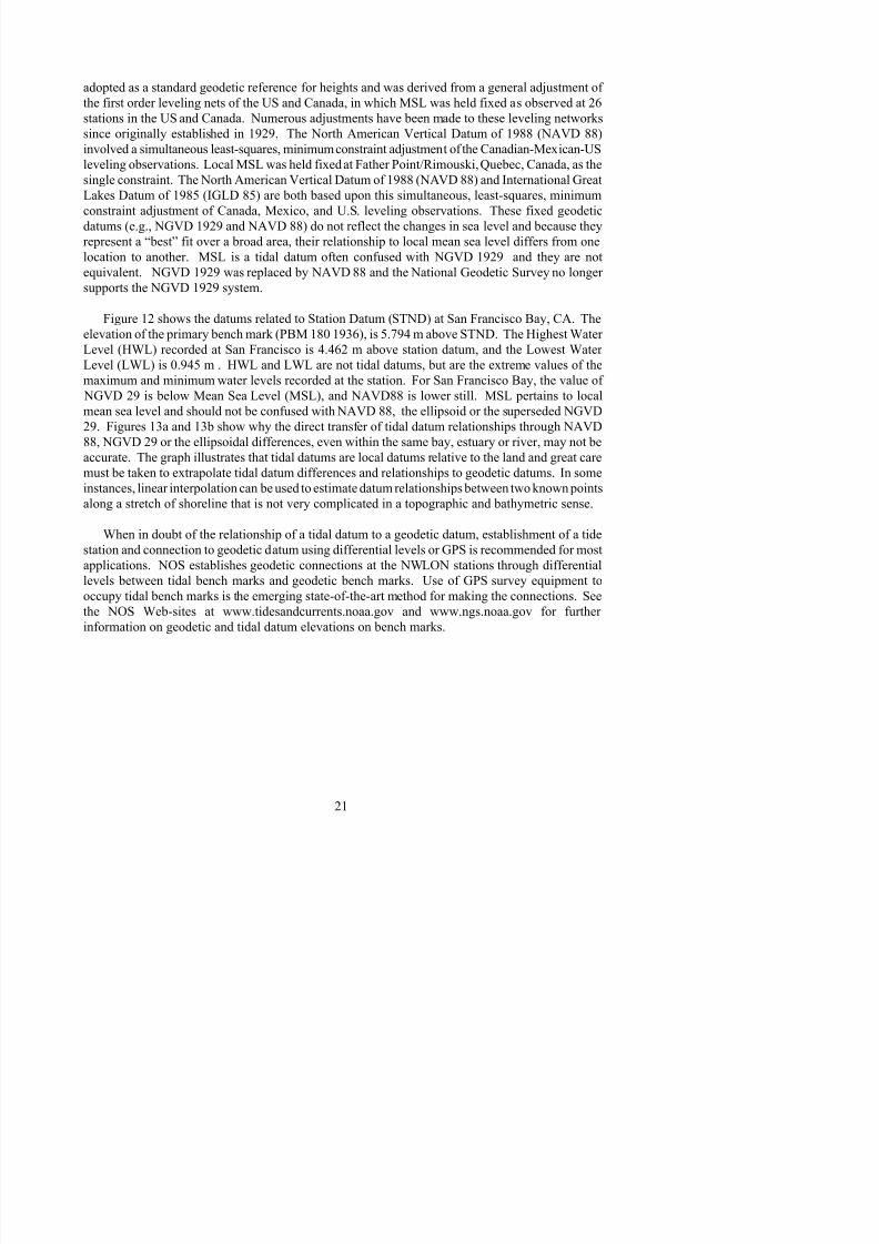
Figure 12 shows the datums related to Station Datum (STND) at San Francisco Bay, CA. The
elevation of the primary bench mark (PBM 180 1936), is 5.794 m above STND. The Highest Water
Level (HWL) recorded at San Francisco is 4.462 m above station datum, and the Lowest Water
Level (LWL) is 0.945 m . HWL and LWL are not tidal datums, but are the extreme values of themaximum and minimum water levels recorded at the station. For San Francisco Bay, the value of
NGVD 29 is below Mean Sea Level (MSL), and NAVD88 is lower still. MSL pertains to local
mean sea level and should not be confused with NAVD 88, the ellipsoid or the superseded NGVD
29. Figures 13a and 13b show why the direct transfer of tidal datum relationships through NAVD
88, NGVD 29 or the ellipsoidal differences, even within the same bay, estuary or river, may not be
accurate. The graph illustrates that tidal datums are local datums relative to the land and great care
must be taken to extrapolate tidal datum differences and relationships to geodetic datums. In some
instances, linear interpolation can be used to estimate datum relationships between two known pointsalong a stretch of shoreline that is not very complicated in a topographic and bathymetric sense.
When in doubt of the relationship of a tidal datum to a geodetic datum, establishment of a tide
station and connection to geodetic datum using differential levels or GPS is recommended for most
applications. NOS establishes geodetic connections at the NWLON stations through differential
levels between tidal bench marks and geodetic bench marks. Use of GPS survey equipment to
occupy tidal bench marks is the emerging state-of-the-art method for making the connections. Seethe NOS Web-sites at www.tidesandcurrents.noaa.gov and www.ngs.noaa.gov for further
information on geodetic and tidal datum elevations on bench marks.

8/6/2019 Computational Techniques for Tidal Datums Handbook
http://slidepdf.com/reader/full/computational-techniques-for-tidal-datums-handbook 36/113
Figure 12. A tidal datum stick diagram for San Francisco, CA showing the
relationships of the various tidal and geodetic datums.

8/6/2019 Computational Techniques for Tidal Datums Handbook
http://slidepdf.com/reader/full/computational-techniques-for-tidal-datums-handbook 37/113
Figure 13a. Locations of stations plotted in Figure 13b.
8/6/2019 Computational Techniques for Tidal Datums Handbook
http://slidepdf.com/reader/full/computational-techniques-for-tidal-datums-handbook 38/113
Tidal Da tums and NG VD Re lative to NAVD88
at Saint Johns River, Florida
-1.50
-0.50
0.50
J a c k s o n v i l l e B e a c h
8 7 2 - 0 2 9 1
L i t t l e T a l b o t I s l a n d
8 7 2 - 0 1 9 4
M a y p o r t
8 7 2 - 0 2 2 0
F u l t o n
8 7 2 - 0 2 2 1
D a m e P o i n t
8 7 2 - 0 2 1 9
M a i n S t . B r i d g e
8 7 2 - 0 2 2 6
L o n g b r a n c h
8 7 2 - 0 2 4 2
O r t e g a R i v e r E n t .
8 7 2 - 0 2 9 6
O r a n g e P a r k
8 7 2 - 0 3 7 4
G
r e e n C o v e S p r i n g s
8 7 2 - 0 4 9 6
P a l a t k a
8 7 2 - 0 7 7 4
Station
E l e v a t i o
n i n M e t e r s
NAVD88
MHW r elative to NA V D88
MSL relative to NAV D88
MLLW relative to NA V D88
NGVD relative to NA V D88
Figure 13b. The relationship of the geodetic datums to tidal datums in the St. John’s River, FL.
The perspective is going upstream from left to right. The graph was constructed by assigning
NAVD88 t l ti l t h it d dj ti th th d t di l
8/6/2019 Computational Techniques for Tidal Datums Handbook
http://slidepdf.com/reader/full/computational-techniques-for-tidal-datums-handbook 39/113
3.3 Steps Required to Compute Tidal Datums at Short-Term Stations
Due to time and resource constraints, primary determinations of tidal datums ( i.e. using 19 years
of data) are not practical at every location along the entire coast where tidal datums are required. At
intermediate locations, a secondary determination of tidal datums can usually be made using
observations covering much shorter periods than 19 years. Results are corrected to an equivalent
mean value by comparison with a suitable control tide station (Marmer, 1951).
Conceptually, the following steps need to be completed in order to compute equivalent NTDE
tidal datums listed in section 3.1 at short term stations using the method of comparison of
simultaneous observations:
1) Select the time period over which the simultaneous comparison will be made.
2) Select the appropriate control tide station for the subordinate station of interest based on
location, tidal characteristics, and availability of data.
. 3) Obtain the simultaneous data from subordinate and control stations and obtain or tabulate
the tides and compute monthly means, as appropriate.
4) Obtain the accepted NTDE values of the tidal datums at the control station from NOS via
the CO-OPS Website (www.tidesandcurrents.noaa.gov)
5) Compute the mean differences and/or ratios (as appropriate) in the tidal parameters between
the subordinate and control station over the period of comparison.
6) Apply the mean differences and ratios computed in step 5, above, to the accepted values at
the control station to obtain equivalent or corrected NTDE values for the subordinate
station. The computations use slightly different formulas depending on the type of tide.
These differences are explained in section 3.4 and in Chapter 4.
3.4 Datum Computation Methods
There are some key datum computation methods used by NOS (in step 6, above) that differ
slightly depending upon the tidal characteristics and the type of tide.
Standard Method. This method is generally used for the West Coast and Pacific Island stations
and is also called the Range Ratio Method. First, equivalent NTDE values for MTL, Mn, DHQ and
DLQ are determined by comparison with an appropriate control. From these, the following are then
computed:
8/6/2019 Computational Techniques for Tidal Datums Handbook
http://slidepdf.com/reader/full/computational-techniques-for-tidal-datums-handbook 40/113
Modified-Range Ratio Method. This method is generally used for the East Coast, Gulf Coast
and Caribbean Island stations. First, equivalent NTDE values for MTL, DTL, Mn and Gt as
determined by comparison with an appropriate control. The difference from the Standard Method
is that ratios of the DHQ and DLQ values are not used to compute MHHW and MLLW becausenumerically the values are very small for semidiurnal tide areas. A Gt ratio about DTL is used
instead. From these, the following are computed:
MLW = MTL - (0.5 x Mn)
MHW = MLW + Mn
MLLW= DTL - (0.5 x Gt)
MHHW = MLLW + Gt
Direct Method. This method is usually used only when a full range of tidal values are not
available. For example, direct MHW can be computed for situations when low waters are not
recorded, such as in the upper reaches of a marsh. Since MTL, DTL, and Mn and Gt cannot be
determined if low waters are cut-off, equivalent NTDE values for MHW and MHHW datums are
determined directly by comparison of high tides with an appropriate control using the available part
of the tidal cycle.
3.5 Accuracy
Generalized accuracies for datums computed at secondary or tertiary stations in terms of the
standard deviation error for the length of the record are summarized in Table 1 (see Swanson, 1974).
These values were calculated using accepted datums for control station pairs in the NWLON. The
values in Table 1 are the confidence intervals for the tidal datums based on the standard deviation.
Table 1. Generalized accuracy of tidal datums for East, Gulf, and West Coasts when determined
from short series of record and based on the standard deviation( one-sigma). From Swanson (1974).
Series Length
(months)
East Coast
(cm) (ft.)
Gulf Coast
(cm) (ft.)
West Coast
(cm) (ft.)
1 3.96 0.13 5.48 0.18 3.96 0.13
3 3.05 0.10 4.57 0.15 3.35 0.11
6 2.13 0.07 3.65 0.12 2.43 0.08
12 1.52 0.05 2.74 0.09 1.82 0.06
8/6/2019 Computational Techniques for Tidal Datums Handbook
http://slidepdf.com/reader/full/computational-techniques-for-tidal-datums-handbook 41/113
Estimated Error in Tidal Datums vs. Length of Series
0.0000.010
0.020
0.030
0.040
0.050
0.060
0.070
0 2 4 6 8 1 0
1 2
1 4
TIME (months)
O n
e - S t a n d a r d D e v i a t i o n
( m e t e r s )
East Coast
Gulf Coast
West Coast
Figure 14. Estimated Error in Tidal Datums from Swanson (1974)
row of Table 1. Examples containing a year of data have generalized errors that correspond to the
fourth row.
The uncertainty in the value of the tidal datum translates into a horizontal uncertainty of the location
of a marine boundary when the tidal datum line is surveyed to the land (Demarcating and Mapping
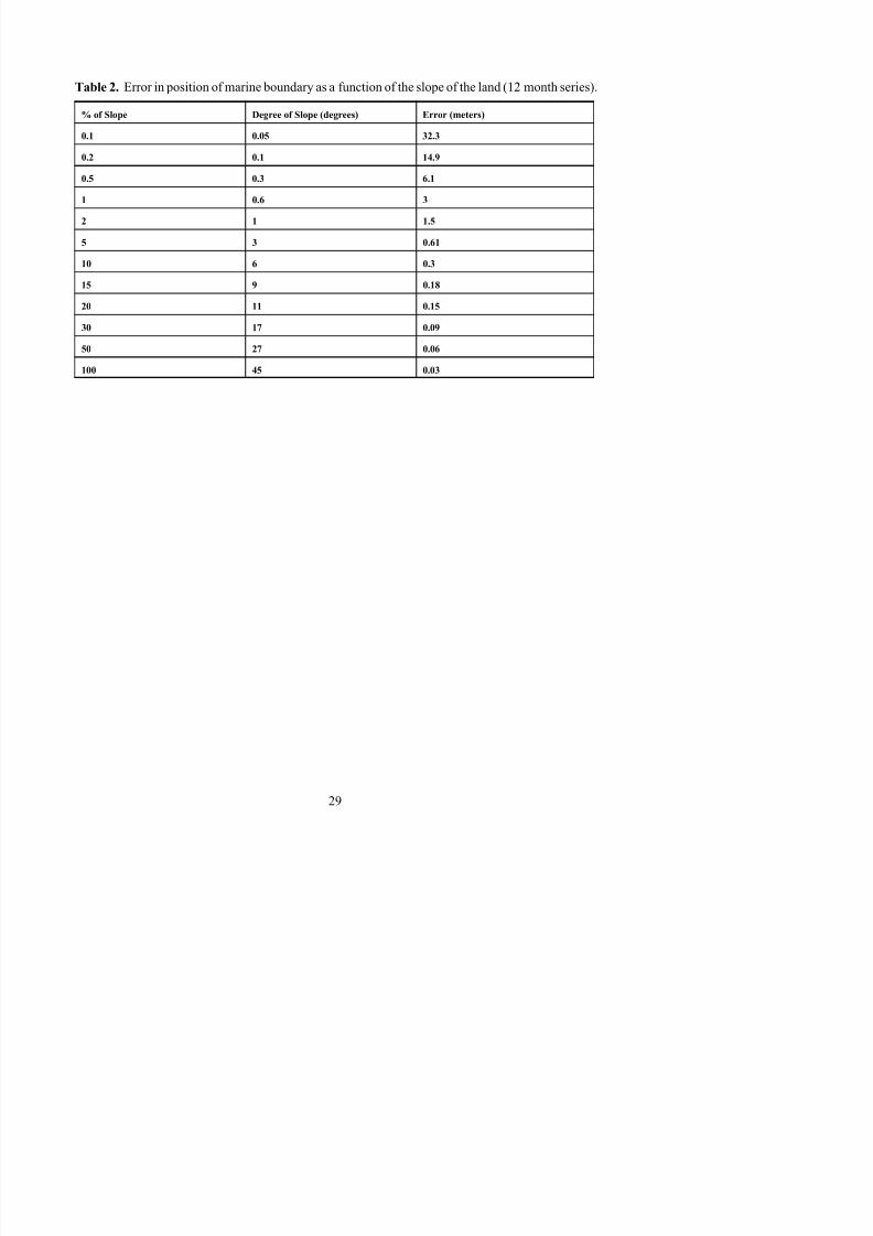
Tidal Boundaries, 1970). Table 2 expresses the uncertainty in the marine boundary as a function
of the slope of the land. A slope of 1% means that the land rises 1 meter for every 100 meters of
horizontal distance. This is illustrated in Figure 15.
8/6/2019 Computational Techniques for Tidal Datums Handbook
http://slidepdf.com/reader/full/computational-techniques-for-tidal-datums-handbook 42/113
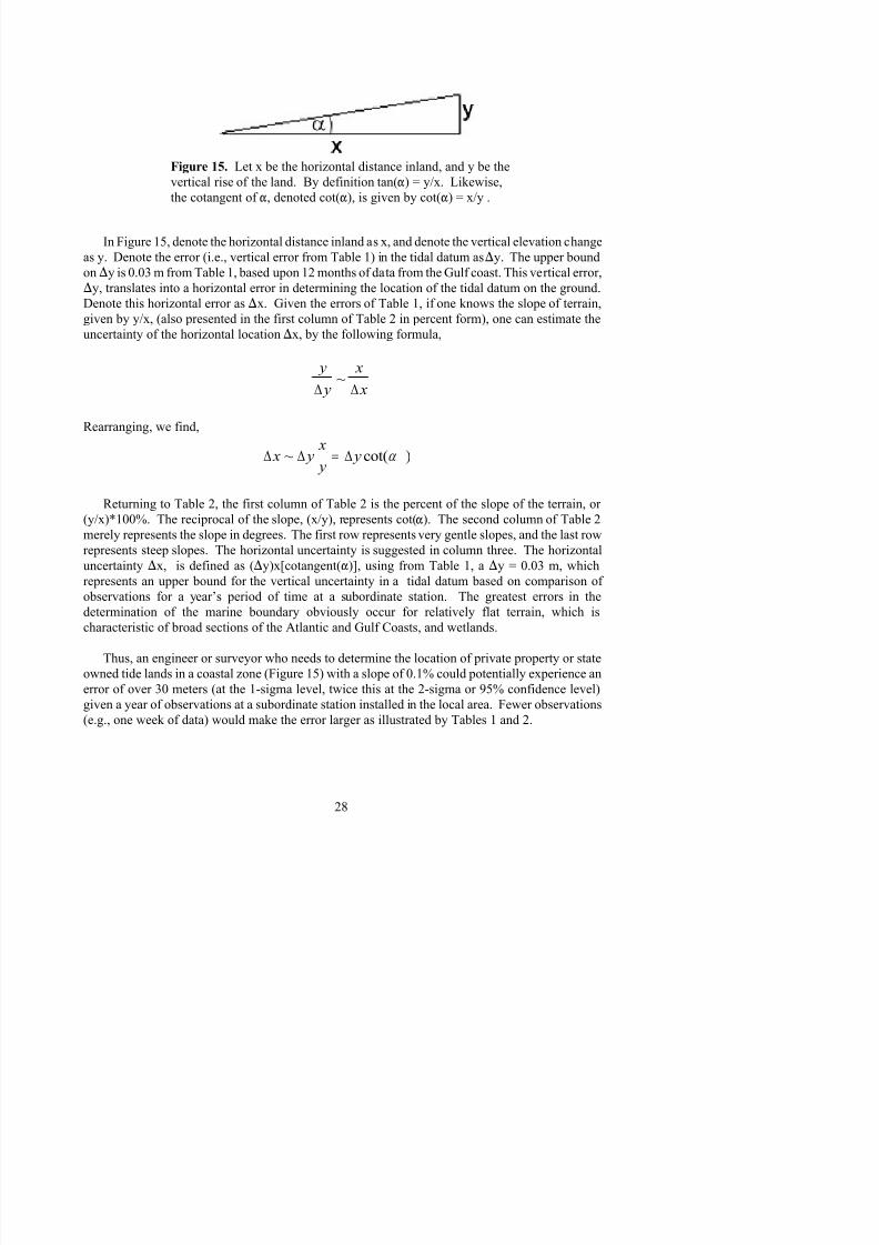
Figure 15. Let x be the horizontal distance inland, and y be the
vertical rise of the land. By definition tan(") = y/x. Likewise,
the cotangent of ", denoted cot("), is given by cot(") = x/y .
y y
x x∆ ∆
~
∆ ∆ ∆ x y x
y y~ cot(= α )
In Figure 15, denote the horizontal distance inland as x, and denote the vertical elevation change
as y. Denote the error (i.e., vertical error from Table 1) in the tidal datum as)y. The upper bound
on)y is 0.03 m from Table 1, based upon 12 months of data from the Gulf coast. This vertical error,
)y, translates into a horizontal error in determining the location of the tidal datum on the ground.
Denote this horizontal error as )x. Given the errors of Table 1, if one knows the slope of terrain,
given by y/x, (also presented in the first column of Table 2 in percent form), one can estimate the
uncertainty of the horizontal location )x, by the following formula,
Rearranging, we find,
Returning to Table 2, the first column of Table 2 is the percent of the slope of the terrain, or
(y/x)*100%. The reciprocal of the slope, (x/y), represents cot("). The second column of Table 2
merely represents the slope in degrees. The first row represents very gentle slopes, and the last row
represents steep slopes. The horizontal uncertainty is suggested in column three. The horizontal
uncertainty )x, is defined as ()y)x[cotangent(")], using from Table 1, a )y = 0.03 m, which
represents an upper bound for the vertical uncertainty in a tidal datum based on comparison of
observations for a year’s period of time at a subordinate station. The greatest errors in the
determination of the marine boundary obviously occur for relatively flat terrain, which is
characteristic of broad sections of the Atlantic and Gulf Coasts, and wetlands.
Thus, an engineer or surveyor who needs to determine the location of private property or state
owned tide lands in a coastal zone (Figure 15) with a slope of 0 1% could potentially experience an
8/6/2019 Computational Techniques for Tidal Datums Handbook
http://slidepdf.com/reader/full/computational-techniques-for-tidal-datums-handbook 43/113
Table 2. Error in position of marine boundary as a function of the slope of the land (12 month series).
% of Slope Degree of Slope (degrees) Error (meters)
0.1 0.05 32.3
0.2 0.1 14.9
0.5 0.3 6.1
1 0.6 3
2 1 1.5
5 3 0.61
10 6 0.3
15 9 0.18
20 11 0.15
30 17 0.09
50 27 0.06
100 45 0.03

8/6/2019 Computational Techniques for Tidal Datums Handbook
http://slidepdf.com/reader/full/computational-techniques-for-tidal-datums-handbook 44/113

8/6/2019 Computational Techniques for Tidal Datums Handbook
http://slidepdf.com/reader/full/computational-techniques-for-tidal-datums-handbook 45/113
4. WORKED EXAMPLES OF TIDAL DATUMS
4.1 Procedural Steps
The procedural steps required to compute tidal datums at short-term stations are illustrated in
this manual using examples. The first three examples illustrate the method of comparison of
simultaneous observations using monthly means from a control and subordinate station in a region
of similar tidal characteristics to produce equivalent datums at the subordinate station. Even though
these examples use 12 months of data, data sets with more or less months use the same procedure.
The second three examples cover the three types of tide using the tide by tide comparison (TBYT)
procedure. These are computed by comparison of individual simultaneous high and low waters
between the tertiary station and a primary control, or an acceptable secondary control station, in aregion of similar tidal characteristics. The last example is one that shows the use of the direct
comparison of mean values for high water datum determination.
The examples found in this Chapter provide details of the formulas and procedures required to
complete steps 4 through 6 found in Section 3.3. Note that the Standard Method is used on the
West Coast, and the Modified Range Ratio method is used for a Gulf Coast example (see section
3.4). The Modified Range Ratio method was adopted procedurally for both diurnal and semidiurnal
tide types because the ratios formed from numerically small ranges of tide and small inequalitiesusing the Standard Method become inconsistent from month to month. So in these cases MHHW
and MLLW are computed using DTL and Gt.
4.2 Comparison of Monthly Means
4.2.1 Modified Range Ratio Method - Semidiurnal Tides
The first example describes computing tidal datums for secondary stations with a semidiurnal
tide. The procedure involves selecting a suitable control station with known 19-year values of thedatums, and reducing the subordinate station data to equivalent 19-year mean values. Along the East
Coast of the United States the tides are predominantly semidiurnal over large distances of the coast,
and many candidate example cases exist. A simple case is offered by the comparison of Fort
Pulaski, GA to Charleston, SC. Their locations are shown in Figure 16. For this example, Fort
Pulaski is being treated as the subordinate station for which datums need to be computed and
Charleston is being treated as the control station.
8/6/2019 Computational Techniques for Tidal Datums Handbook
http://slidepdf.com/reader/full/computational-techniques-for-tidal-datums-handbook 46/113
8/6/2019 Computational Techniques for Tidal Datums Handbook
http://slidepdf.com/reader/full/computational-techniques-for-tidal-datums-handbook 47/113
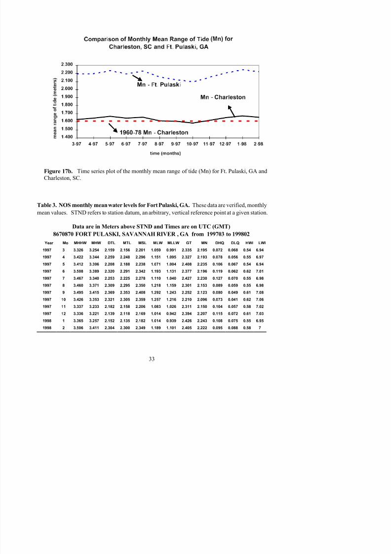
Figure 17b. Time series plot of the monthly mean range of tide (Mn) for Ft. Pulaski, GA and
Charleston, SC.
Table 3. NOS monthly mean water levels for Fort Pulaski, GA. These data are verified, monthly
mean values. STND refers to station datum, an arbitrary, vertical reference point at a given station.
Data are in Meters above STND and Times are on UTC (GMT)
8670870 FORT PULASKI, SAVANNAH RIVER , GA from 199703 to 199802
Year Mo MHHW MHW DTL MTL MSL MLW MLLW GT MN DHQ DLQ HWI LWI
1997 3 3.326 3.254 2.159 2.156 2.201 1.059 0.991 2.335 2.195 0.072 0.068 0.54 6.94
1997 4 3.422 3.344 2.259 2.248 2.296 1.151 1.095 2.327 2.193 0.078 0.056 0.55 6.97
1997 5 3.412 3.306 2.208 2.188 2.238 1.071 1.004 2.408 2.235 0.106 0.067 0.54 6.94
1997 6 3.508 3.389 2.320 2.291 2.342 1.193 1.131 2.377 2.196 0.119 0.062 0.62 7.01
1997 7 3.467 3.340 2.253 2.225 2.278 1.110 1.040 2.427 2.230 0.127 0.070 0.55 6.98
1997 8 3.460 3.371 2.309 2.295 2.350 1.218 1.159 2.301 2.153 0.089 0.059 0.55 6.98
1997 9 3.495 3.415 2.369 2.353 2.408 1.292 1.243 2.252 2.123 0.080 0.049 0.61 7.08
1997 10 3.426 3.353 2.321 2.305 2.359 1.257 1.216 2.210 2.096 0.073 0.041 0.62 7.06
8/6/2019 Computational Techniques for Tidal Datums Handbook
http://slidepdf.com/reader/full/computational-techniques-for-tidal-datums-handbook 48/113
MTL MHW MLW = +2
. (1)
Table 4. NOS monthly mean water levels for Charleston, SC. These data are verified, monthly
mean values. The data fields have the same meaning as in Table3.
Data are in Meters above STND and Times are on UTC (GMT)
8665530 CHARLESTON, COOPER RIVER ENTRANCE , SC from 199703 to 199802
Year Mo MHHW MHW DTL MTL MSL MLW MLLW GT MN DHQ DLQ HWI LWI
1997 3 2.555 2.476 1.672 1.662 1.700 0.847 0.789 1.766 1.629 0.079 0.058 0.41 6.65
1997 4 2.648 2.574 1.763 1.751 1.797 0.928 0.877 1.771 1.646 0.074 0.051 0.41 6.66
1997 5 2.609 2.506 1.699 1.673 1.717 0.840 0.789 1.820 1.666 0.103 0.051 0.41 6.67
1997 6 2.725 2.614 1.818 1.792 1.836 0.970 0.910 1.815 1.644 0.111 0.060 0.47 6.77
1997 7 2.673 2.557 1.758 1.730 1.774 0.904 0.843 1.830 1.653 0.116 0.061 0.46 6.70
1997 8 2.683 2.595 1.807 1.789 1.832 0.984 0.932 1.751 1.611 0.088 0.052 0.45 6.66
1997 9 2.732 2.654 1.870 1.851 1.896 1.048 1.008 1.724 1.606 0.078 0.040 0.51 6.72
1997 10 2.672 2.600 1.824 1.807 1.851 1.014 0.975 1.697 1.586 0.072 0.039 0.48 6.71
1997 11 2.579 2.478 1.692 1.669 1.709 0.860 0.805 1.774 1.618 0.101 0.055 0.46 6.68
1997 12 2.572 2.459 1.661 1.635 1.673 0.811 0.749 1.823 1.648 0.113 0.062 0.45 6.71
1998 1 2.588 2.471 1.665 1.634 1.678 0.797 0.742 1.846 1.674 0.117 0.055 0.39 6.63
1998 2 2.724 2.637 1.821 1.811 1.854 0.984 0.917 1.807 1.653 0.087 0.067 0.39 6 .7
Table 5. NOS accepted tidal datums for Charleston. Data are accepted. These are the 19-year
values of the tidal datums at Charleston, SC, and have been computed by first reduction.
Data are in Meters above STND, time intervals are on UTC (GMT).
8665530 Charleston, Cooper River Entrance, SC, USA
Station MHHW MHW DTL MTL MSL MLW MLLW GT MN8665530 2.527 2.423 1.643 1.622 1.658 0.817 0.759 1.768 1.606DHQ DLQ HWI LWI
0.104 0.058 0.35 6.57
Definition, MTL. Mean Tide Level, MTL, the average of MHW and MLW, is defined by
the equation
This value is already calculated and is presented in the above Tables 3-5. MTL is the starting
point for the calculation of the equivalent 19 year datums at Fort Pulaski, based on one year of
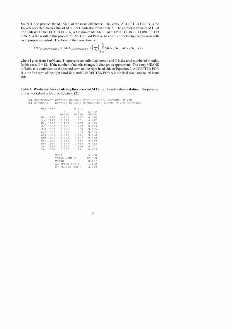
8/6/2019 Computational Techniques for Tidal Datums Handbook
http://slidepdf.com/reader/full/computational-techniques-for-tidal-datums-handbook 49/113
MTL MTL N
(MTL (I) MTL (I)) ( ) I
N
CORRECTED FOR A ACCEPTED FOR B A B= +
−
=∑
12
1
MONTHS to produce the MEANS, or the mean difference. The entry, ACCEPTED FOR B, is the
19-year accepted mean value of MTL for Charleston from Table 5. The corrected value of MTL at
Fort Pulaski, CORRECTED FOR A, is the sum of MEANS + ACCEPTED FOR B. CORRECTED
FOR A is the result of this procedure: MTL at Fort Pulaski has been corrected by comparison withan appropriate control. The form of the correction is
where I goes from 1 to N, and I represents an individual month and N is the total number of months.
In this case, N = 12. If the number of months change, N changes as appropriate. The entry MEANSin Table 6 is equivalent to the second term on the right hand side of Equation 2, ACCEPTED FOR
B is the first term of the right hand side, and CORRECTED FOR A is the final result on the left hand
side.
Table 6. Worksheet for calculating the corrected MTL for the subordinate station. The purpose
of this worksheet is to solve Equation (2).
(A) SUBORDINATE STATION 8670870 FORT PULASKI, SAVANNAH RIVER(B) STANDARD STATION 8665530 CHARLESTON, COOPER RIVER ENTRANCE
Mon Year M T LA B A - B
METER METER METERMar 1997 2.156 1.662 0.494Apr 1997 2.248 1.751 0.497May 1997 2.188 1.673 0.515Jun 1997 2.291 1.792 0.499
Jul 1997 2.225 1.730 0.495Aug 1997 2.295 1.789 0.506Sep 1997 2.353 1.851 0.502Oct 1997 2.305 1.807 0.498Nov 1997 2.158 1.669 0.489Dec 1997 2.118 1.635 0.483Jan 1998 2.135 1.634 0.501Feb 1998 2.300 1.811 0.489
SUMS 5.968TOTAL MONTHS 12.000
MEANS 0.497ACCEPTED FOR B 1.622CORRECTED FOR A 2.119

8/6/2019 Computational Techniques for Tidal Datums Handbook
http://slidepdf.com/reader/full/computational-techniques-for-tidal-datums-handbook 50/113
DTL DTL N
(DTL (I) DTL (I)) I
N ( ).CORRECTED FOR A ACCEPTED FOR B A B= +
−
=∑
1
14
DTL MHHW MLLW = +2
. (3)
Definition, DTL. Diurnal Tide Level, DTL, is defined as
DTL is also provided in Tables 3-5 using the above Equation 3 from the MHHW and MLLW
data in those tables, and is entered into Table 7 below. In Table 7, Column A is DTL from the
values in Table 3. Column B is DTL from values in Table 4. The third column in Table 7 is the
difference field A-B. The difference field is summed and stored in SUMS, the mean is computed
and stored in MEANS. The ACCEPTED FOR B entry for DTL is obtained from Table 5. Thecorrected DTL value at Fort Pulaski is the sum of MEANS + ACCEPTED FOR B, and is stored in
CORRECTED FOR A entry of Table 7. The mathematical form of the correction is given by
Equation 4,
Table 7. Worksheet for calculating the corrected DTL for a subordinate station. This
worksheet solves Equation 4.
Mon Year DTLA B A - B
METER METER METERMar 1997 2.159 1.672 0.487
Apr 1997 2.259 1.763 0.496May 1997 2.208 1.699 0.509Jun 1997 2.320 1.818 0.502Jul 1997 2.253 1.758 0.495Aug 1997 2.309 1.807 0.502Sep 1997 2.369 1.870 0.499Oct 1997 2.321 1.824 0.497Nov 1997 2.182 1.692 0.490Dec 1997 2.139 1.661 0.478Jan 1998 2.152 1.665 0.487Feb 1998 2.304 1.821 0.483
SUMS 5.925TOTAL MONTHS 12.000MEANS 0.494ACCEPTED FOR B 1.643CORRECTED FOR A 2.137

8/6/2019 Computational Techniques for Tidal Datums Handbook
http://slidepdf.com/reader/full/computational-techniques-for-tidal-datums-handbook 51/113
Mn Mn N
Mn I
Mn I CORRECTED FOR A ACCEPTED FOR B
A
B I
N
(6).= ×
=
∑1
1
( )
( )
Definition, MN. The Mean Range, Mn, is defined by
(5).n HW LW = −
Mn is given in Tables 3-5 and was calculated by applying the above equation. The results are
organized in Table 8 below. Column A is the Mn from Table 3 and Column B is the Mn acquired
from Table 4. Column A/B is the ratio of the values in Column A divided by those in Column B.
The sum of the ratios is stored in SUMS. The mean ratio is stored in MEANS. The accepted value
of Mn from Charleston is obtained from Table 5. The corrected value for Mn at Fort Pulaski is
determined by multiplying ACCEPTED FOR B by MEANS, and is shown in CORRECTED FOR A in Table 8. The mathematical form of the correction is represented by Equation 6,
Table 8. Worksheet for correcting the Mn at a subordinate station. This worksheet solvesEquation 6.
Mon Year MnA B A / B
METER METER RATIOMar 1997 2.195 1.629 1.347Apr 1997 2.193 1.646 1.332May 1997 2.235 1.666 1.342Jun 1997 2.196 1.644 1.336
Jul 1997 2.230 1.653 1.349Aug 1997 2.153 1.611 1.336Sep 1997 2.123 1.606 1.322Oct 1997 2.096 1.586 1.322Nov 1997 2.150 1.618 1.329Dec 1997 2.207 1.648 1.339Jan 1998 2.243 1.674 1.340Feb 1998 2.222 1.653 1.344
SUMS 16.038TOTAL MONTHS 12.000MEANS 1.337ACCEPTED FOR B 1.606CORRECTED FOR A 2.146
h i l ( ) i d fi d

8/6/2019 Computational Techniques for Tidal Datums Handbook
http://slidepdf.com/reader/full/computational-techniques-for-tidal-datums-handbook 52/113
Gt Gt N
Gt I
Gt I CORRECTED FOR A ACCEPTED FOR B
A
B I
N
(8).= ×
=
∑1
1
( )
( )
In Table 9 below the values of Gt are obtained from Table 3 and Table 4. The Column A/B is
the ratio of the values in Column A divided by the values in Column B. The A/B column is summed
and the mean ratio determined. The accepted Gt at Charleston is obtained from Table 5. TheCORRECTED for A is the product of MEANS times ACCEPTED for B. The mathematical form
of the corrected Gt is given by Equation 8,
Table 9. Worksheet for calculating the corrected Gt at a subordinate station. The purpose of
this worksheet is to solve Equation 8.
Mon Year G tA B A / B
METER METER RATIOMar 1997 2.335 1.766 1.322
Apr 1997 2.327 1.771 1.314May 1997 2.408 1.820 1.323Jun 1997 2.377 1.815 1.310Jul 1997 2.427 1.830 1.326Aug 1997 2.301 1.751 1.314Sep 1997 2.252 1.724 1.306Oct 1997 2.210 1.697 1.302Nov 1997 2.311 1.774 1.303Dec 1997 2.394 1.823 1.313Jan 1998 2.426 1.846 1.314
Feb 1998 2.405 1.807 1.331
SUMS 15.778TOTAL MONTHS 12.000MEANS 1.315ACCEPTED FOR B 1.768CORRECTED FOR A 2.325
Once the corrected values of MTLCORRECTED FOR A, DTLCORRECTED FOR A, Mn CORRECTED FOR A, and
Gt CORRECTED FOR A, are determined by the above process the following Equations 9-12 may be used
to determine the tidal datums at the subordinate station.
I h f th f ti b th i l l f MTL
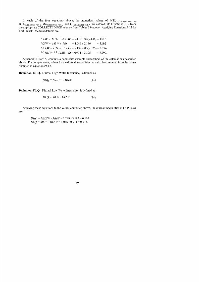
8/6/2019 Computational Techniques for Tidal Datums Handbook
http://slidepdf.com/reader/full/computational-techniques-for-tidal-datums-handbook 53/113
MLW MTL Mn
MHW MLW Mn
MLLW DTL Gt
HHW LLW Gt
= − × = − =
= + = + =
= − × = − =
= + = + =
05 2119 05 2146 1046
1046 2146 3192
05 2137 05 2 325 0 974
0 974 2 325 3299
. . . ( . ) .
. . .
. . . ( . ) .
. . . .
In each of the four equations above, the numerical values of MTLCORRECTED FOR A,
DTLCORRECTED FOR A, MnCORRECTED FOR A, and GTCORRECTED FOR A, are entered into Equations 9-12 from
the appropriate CORRECTED FOR A entry from Tables 6-9 above. Applying Equations 9-12 for
Fort Pulaski, the tidal datums are
Appendix 1. Part A, contains a composite example spreadsheet of the calculations described
above. For completeness, values for the diurnal inequalities may also be computed from the values
obtained in equations 9-12.
Definition, DHQ. Diurnal High Water Inequality, is defined as
DHQ = MHHW - MHW. (13)
Definition, DLQ. Diurnal Low Water Inequality, is defined as
DLQ = MLW - MLLW . (14)
Applying these equations to the values computed above, the diurnal inequalities at Ft. Pulaski
are
DHQ = MHHW - MHW = 3.299 - 3.192 = 0.107
DLQ = MLW - MLLW = 1.046 - 0.974 = 0.072.
4 2 2 M difi d R R ti M th d Di l Tid

8/6/2019 Computational Techniques for Tidal Datums Handbook
http://slidepdf.com/reader/full/computational-techniques-for-tidal-datums-handbook 54/113
Figure 18. A map showing tide stations in the Gulf of Mexico.
4.2.2 Modified Range Ratio Method - Diurnal Tides
Along much the Gulf Coast of the United States the tides are predominantly diurnal. However,
over short distances of the coast, the tides may in one location be diurnal, and in another location
nearby, semidiurnal or mixed. Few easy candidate example cases exist. However, a simple case is
offered by the comparison of Panama City Beach, FL to Pensacola, FL, as shown in Figure 18.
From the CO-OPS website, http://www.tidesandcurrents.noaa.gov/, verified historical monthly
mean water level data, and accepted datums, may be downloaded. A year’s worth of monthly values
for Panama City Beach and Pensacola are shown in Tables 10 and 11. A subset of these monthly
mean values are plotted in the graphs found in Figures 19a and 19b. These data were downloaded
from the hyperlink U.S. and Global Coastal Stations, under Verified/Historical Water Level Data.The equations used to compute the tidal datums at the subordinate station, Panama City Beach, have
been completely developed in the previous section on semidiurnal tides, and are applied in a
straightforward manner to diurnal tides.
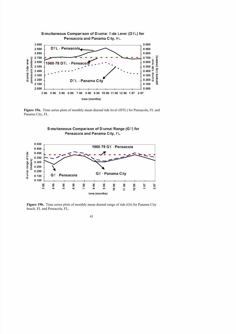
8/6/2019 Computational Techniques for Tidal Datums Handbook
http://slidepdf.com/reader/full/computational-techniques-for-tidal-datums-handbook 55/113
Figure 19a. Time series plots of monthly mean diurnal tide level (DTL) for Pensacola, FL and
Panama City, FL.
Table 10 NOS monthly mean water levels for Panama City Beach FL
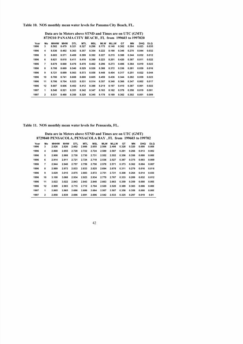
8/6/2019 Computational Techniques for Tidal Datums Handbook
http://slidepdf.com/reader/full/computational-techniques-for-tidal-datums-handbook 56/113
Table 10. NOS monthly mean water levels for Panama City Beach, FL.
Data are in Meters above STND and Times are on UTC (GMT)
8729210 PANAMA CITY BEACH , FL from 199603 to 1997020
Year Mo MHHW MHW DTL MTL MSL MLW MLLW GT MN DHQ DLQ1996 3 8.502 8.479 8.321 8.327 8.298 8.175 8.140 0.362 0.304 0.023 0.035
1996 4 8.536 8.492 8.363 8.357 8.354 8.222 8.190 0.346 0.270 0.044 0.032
1996 5 8.603 8.571 8.409 8.399 8.392 8.227 8.215 0.388 0.344 0.032 0.012
1996 6 8.621 8.610 8.411 8.416 8.399 8.223 8.201 0.420 0.387 0.011 0.022
1996 7 8.679 8.660 8.476 8.478 8.462 8.296 8.273 0.406 0.364 0.019 0.023
1996 8 8.708 8.669 8.540 8.529 8.526 8.388 8.372 0.336 0.281 0.039 0.016
1996 9 8.721 8.699 8.563 8.573 8.558 8.448 8.404 0.317 0.251 0.022 0.044
1996 10 8.780 8.741 8.608 8.600 8.605 8.459 8.436 0.344 0.282 0.039 0.023
1996 11 8.706 8.704 8.523 8.531 8.514 8.357 8.340 0.366 0.347 0.002 0.017
1996 12 8.607 8.606 8.402 8.412 8.388 8.219 8.197 0.410 0.387 0.001 0.022
1997 1 8.540 8.521 8.351 8.342 8.347 8.163 8.162 0.378 0.358 0.019 0.001
1997 2 8.531 8.480 8.350 8.329 8.345 8.178 8.169 0.362 0.302 0.051 0.009
Table 11. NOS monthly mean water levels for Pensacola, FL.
Data are in Meters above STND and Times are on UTC (GMT)8729840 PENSACOLA, PENSACOLA BAY , FL from 199603 to 199702
Year Mo MHHW MHW DTL MTL MSL MLW MLLW GT MN DHQ DLQ1996 3 2.826 2.826 2.662 2.666 2.655 2.506 2.498 0.328 0.320 0.000 0.008
1996 4 2.868 2.855 2.728 2.722 2.724 2.589 2.587 0.281 0.266 0.013 0.002
1996 5 2.908 2.908 2.730 2.730 2.731 2.552 2.552 0.356 0.356 0.000 0.000
1996 6 2.914 2.911 2.721 2.724 2.718 2.536 2.527 0.387 0.375 0.003 0.009
1996 7 2.944 2.940 2.757 2.759 2.750 2.578 2.571 0.373 0.362 0.004 0.007
1996 8 2.989 2.973 2.833 2.833 2.825 2.694 2.678 0.311 0.279 0.016 0.016
1996 9 3.029 3.015 2.875 2.883 2.872 2.751 2.721 0.308 0.264 0.014 0.030
1996 10 3.100 3.068 2.934 2.923 2.934 2.779 2.767 0.333 0.289 0.032 0.012
1996 11 3.022 3.022 2.843 2.843 2.840 2.663 2.663 0.359 0.359 0.000 0.000
1996 12 2 909 2 903 2 715 2 712 2 704 2 520 2 520 0 389 0 383 0 006 0 000
Table 12. NOS accepted tidal datums for Pensacola. These are the 19-year, accepted, official

8/6/2019 Computational Techniques for Tidal Datums Handbook
http://slidepdf.com/reader/full/computational-techniques-for-tidal-datums-handbook 57/113
Table 12. NOS accepted tidal datums for Pensacola. These are the 19 year, accepted, official
values of the tidal datums at Pensacola, FL, and have been computed by first reduction. Note that
HWI -- Greenwich Mean High Water Interval in Hours, and LWI -- Greenwich Mean Low Water
Interval in Hours, are not calculated for this station because the type of tide at Pensacola is diurnal.The data are in meters above station datum.
Data are in Meters above STND
8729840 Pensacola, Pensacola Bay, FL, USA
Station MHHW MHW DTL MTL MSL MLW MLLW GT MN
8729840 2.911 2.902 2.719 2.719 2.713 2.536 2.524 0.387 0.366
DHQ DLQ HWI LWI
0.009 0.012 N/A N/A
Corrected MTL for Panama City Beach. Mean Tide Level, MTL, the average of MHW and
MLW, is defined by Equation 1, and is presented in the above Tables 10-12. MTL is the starting
point for the calculation of the equivalent 19 year datums at Panama City Beach, based on one year
of monthly means between there and Pensacola. The subordinate station, Panama City Beach, is
designated as station A, and the control station, Pensacola is designated station B. MTL at Panama
City Beach must be reduced to a 19-year equivalent value by using the information from Pensacola.
In Table 13 below the values in column A are the MTL values from Table 10, those values incolumn B are from Table 11. The column to the right of B, is the difference, A-B. The procedure
is identical to the semidiurnal case and shall be reiterated here. The entry, SUMS, is the sum of the
differences A-B. The SUMS are divided by the TOTAL MONTHS to produce the MEANS, or the
mean differences. The entry, ACCEPTED FOR B, is the accepted value of MTL for Pensacola
from Table 12. The corrected value of MTL at Panama City Beach, CORRECTED FOR A, is the
sum of MEANS + ACCEPTED FOR B. As a result of this procedure MTL observed at Panama
City Beach for the period from March 1996 to February 1997 has been corrected to an equivalent
19-year mean value of MTL by comparison with an appropriate control.
Table 13. Worksheet for calculating the corrected MTL for the subordinate station. The
purpose of this worksheet is to solve Equation (2).
(A) SUBORDINATE STATION 8729210 PANAMA CITY BEACH(B) STANDARD STATION 8729840 PENSACOLA, PENSACOLA BAY
Mon Year M T LA B A - B
METER METER METERMar 1996 8.327 2.666 5.661Apr 1996 8.357 2.722 5.635May 1996 8.399 2.730 5.669
SUMS 68.12112 000

8/6/2019 Computational Techniques for Tidal Datums Handbook
http://slidepdf.com/reader/full/computational-techniques-for-tidal-datums-handbook 58/113
TOTAL MONTHS 12.000MEANS 5.677ACCEPTED FOR B 2.719
CORRECTED FOR A 8.396
Corrected DTL for Panama City Beach. DTL is obtained from Tables 10-12 and entered into
Table 14 below. Column A is DTL from Table 10, Column B is DTL from Table 11, and the third
column is the difference field A-B. The differences are summed and stored in SUMS, the mean is
computed and stored in MEANS. The ACCEPTED FOR B is calculated by applying the above
equation to the MHHW and MLLW entries in Table 12. The corrected DTL value at Panama City
Beach is the sum of MEANS + ACCEPTED FOR B, and is stored in CORRECTED FOR A.
Table 14. Worksheet for calculating the corrected DTL for Panama City Beach. The purpose
of this Table is to solve Equation 4 for Panama City Beach.
Mon Year DTLA B A - B
METER METER METERMar 1996 8.321 2.662 5.659
Apr 1996 8.363 2.728 5.635May 1996 8.409 2.730 5.679Jun 1996 8.411 2.721 5.690Jul 1996 8.476 2.757 5.719Aug 1996 8.540 2.833 5.707Sep 1996 8.563 2.875 5.688Oct 1996 8.608 2.934 5.674Nov 1996 8.523 2.843 5.680Dec 1996 8.402 2.715 5.687Jan 1997 8.351 2.686 5.665Feb 1997 8.350 2.696 5.654
SUMS 68.137TOTAL MONTHS 12.000MEANS 5.678ACCEPTED FOR B 2.719CORRECTED FOR A 8.397
Corrected MN for Panama City Beach. The Mean Range, Mn, is defined by Equation 5 and
is obtained from Tables 10-12. The results are organized in Table 15 below.
Table 15. Worksheet for correcting the Mn at a subordinate station.
Mon Year M N
Oct 1996 0.282 0.289 0.976N 1996 0 347 0 359 0 967
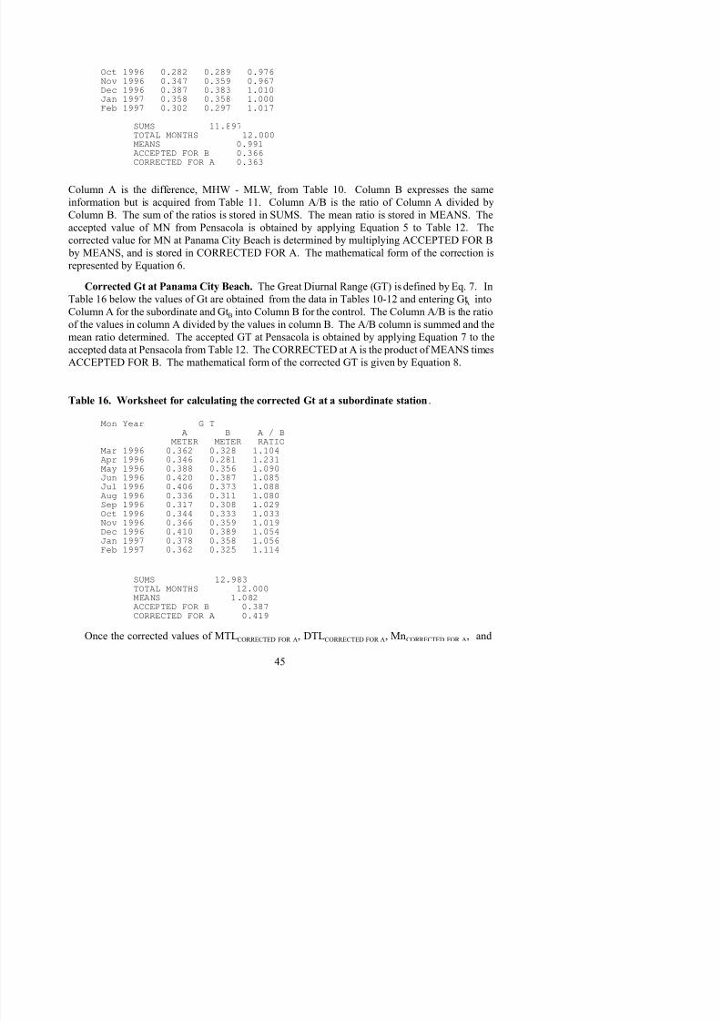
8/6/2019 Computational Techniques for Tidal Datums Handbook
http://slidepdf.com/reader/full/computational-techniques-for-tidal-datums-handbook 59/113
Nov 1996 0.347 0.359 0.967Dec 1996 0.387 0.383 1.010Jan 1997 0.358 0.358 1.000
Feb 1997 0.302 0.297 1.017
SUMS 11.897TOTAL MONTHS 12.000MEANS 0.991ACCEPTED FOR B 0.366CORRECTED FOR A 0.363
Column A is the difference, MHW - MLW, from Table 10. Column B expresses the same
information but is acquired from Table 11. Column A/B is the ratio of Column A divided by
Column B. The sum of the ratios is stored in SUMS. The mean ratio is stored in MEANS. The
accepted value of MN from Pensacola is obtained by applying Equation 5 to Table 12. The
corrected value for MN at Panama City Beach is determined by multiplying ACCEPTED FOR B
by MEANS, and is stored in CORRECTED FOR A. The mathematical form of the correction is
represented by Equation 6.
Corrected Gt at Panama City Beach. The Great Diurnal Range (GT) is defined by Eq. 7. In
Table 16 below the values of Gt are obtained from the data in Tables 10-12 and entering GtA
into
Column A for the subordinate and GtB into Column B for the control. The Column A/B is the ratio
of the values in column A divided by the values in column B. The A/B column is summed and the
mean ratio determined. The accepted GT at Pensacola is obtained by applying Equation 7 to the
accepted data at Pensacola from Table 12. The CORRECTED at A is the product of MEANS times
ACCEPTED FOR B. The mathematical form of the corrected GT is given by Equation 8.
Table 16. Worksheet for calculating the corrected Gt at a subordinate station.
Mon Year G TA B A / B
METER METER RATIOMar 1996 0.362 0.328 1.104Apr 1996 0.346 0.281 1.231May 1996 0.388 0.356 1.090Jun 1996 0.420 0.387 1.085Jul 1996 0.406 0.373 1.088Aug 1996 0.336 0.311 1.080Sep 1996 0.317 0.308 1.029Oct 1996 0.344 0.333 1.033Nov 1996 0.366 0.359 1.019Dec 1996 0.410 0.389 1.054Jan 1997 0.378 0.358 1.056Feb 1997 0.362 0.325 1.114
GTCORRECTED FOR A, are determined by the above process the Equations 9-12 may be used to determine
8/6/2019 Computational Techniques for Tidal Datums Handbook
http://slidepdf.com/reader/full/computational-techniques-for-tidal-datums-handbook 60/113
MLW MTL Mn
MHW MLW Mn
MLLW DTL Gt
HHW LLW Gt
= − × = − =
= + = + =
= − × = − =
= + = + =
05 8 396 05 0 363 8 214
8 214 0 363 8577
05 8 397 05 0 419 8188
8188 0 419 8 607
. . . ( . ) .
. . .
. . . ( . ) .
. . . .
the other tidal datums at the subordinate station. For Panama City Beach, the tidal datums are
4.2.3 Standard Method - Mixed Tides
The mixed tides case requires methodology called the standard method (section 3.4). Like the
previous cases, the problem involves selecting a suitable control station with known 19-year mean
values of the datums, and reducing the subordinate station data to their equivalent 19-year mean.
Along the West Coast of the United States the tides are predominantly mixed over large distances
of the coast, and many candidate example cases exist. A simple case is offered by the comparison
of Alameda, CA (subordinate station) to San Francisco, CA (control station), both located in central
California within San Francisco Bay (see Figure 20.) From the CO-OPS website,http://www.tidesandcurrents.noaa.gov/, verified and historical monthly mean water level data, and
accepted datums, may be downloaded. A year’s worth of monthly values for Alameda and San
Francisco are shown in Tables 17 - 19 and monthly mean values for MTL and Mn are plotted in
Figures 21a and 21b. This data is downloaded from the hyperlink U.S. and Global Coastal Stations,
under Verified/Historical Water Level Data. A full example computational spreadsheet for the full
comparison is found in Appendix 1.

8/6/2019 Computational Techniques for Tidal Datums Handbook
http://slidepdf.com/reader/full/computational-techniques-for-tidal-datums-handbook 61/113
Figure 20. Map of California showing the locations of NWLON stations.
Simultaneous Comparison of Mean Tide Level (MTL) for San
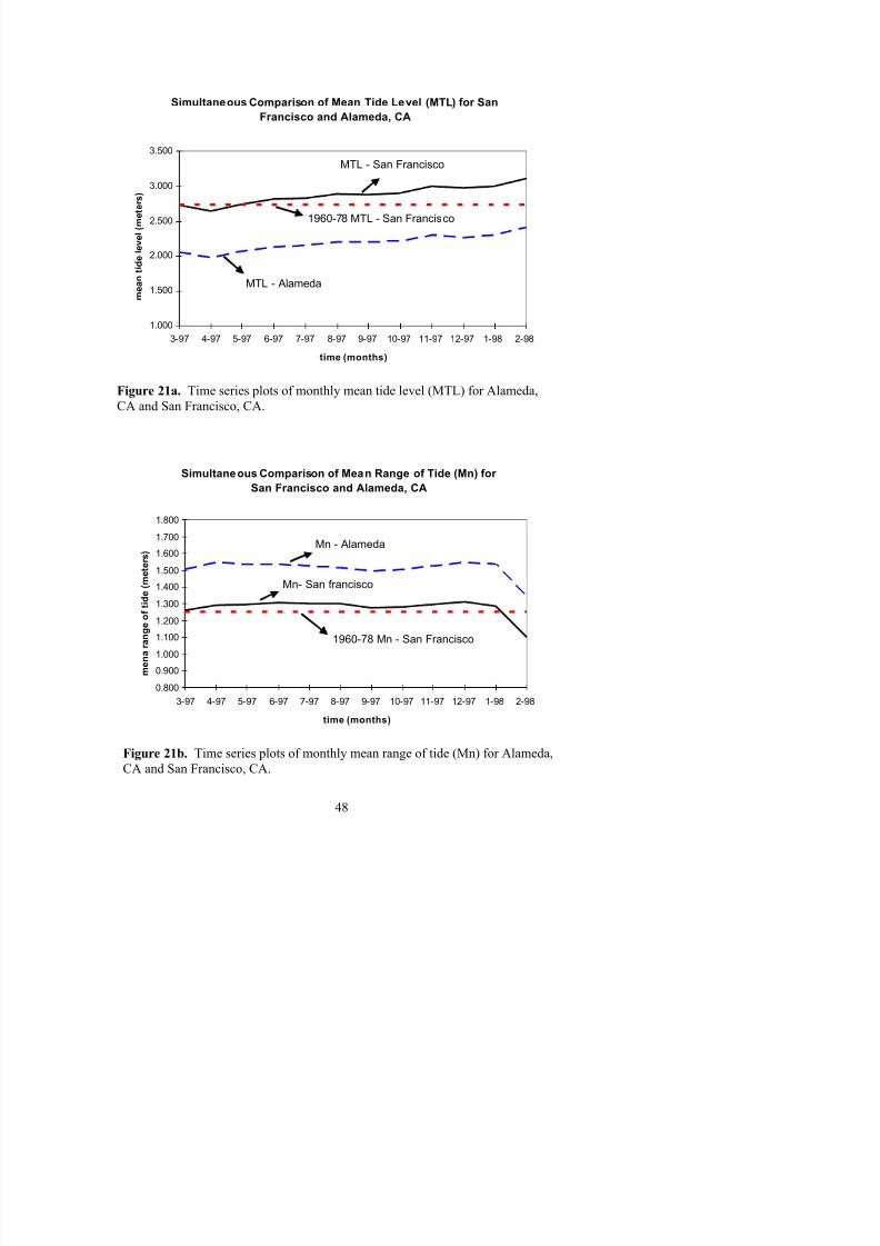
8/6/2019 Computational Techniques for Tidal Datums Handbook
http://slidepdf.com/reader/full/computational-techniques-for-tidal-datums-handbook 62/113
Simultaneous Comparison of Mean Tide Level (MTL) for San
Francisco and Alameda, CA
1.000
1.500
2.000
2.500
3.000
3.500
3-97 4-97 5-97 6-97 7-97 8-97 9-97 10-97 11-97 12-97 1-98 2-98
time (months)
m e a n t i d e l e v e l ( m e t e r s )
MTL - San Francisco
MTL - Alameda
1960-78 MTL - San Francisco
Figure 21a. Time series plots of monthly mean tide level (MTL) for Alameda,
CA and San Francisco, CA.
Simultaneous Comparison of Mean Range of Tide (Mn) for
San Francisco and Alameda, CA
0.900
1.000
1.100
1.200
1.300
1.400
1.500
1.600
1.700
1.800
m e n a r a n g e o f
t i d e ( m e t e r s )
Mn - Alameda
Mn- San francisco
1960-78 Mn - San Francisco
Table 17. NOS monthly mean water levels for Alameda, CA. The data are verified.

8/6/2019 Computational Techniques for Tidal Datums Handbook
http://slidepdf.com/reader/full/computational-techniques-for-tidal-datums-handbook 63/113
Data are in Meters above STND and Times are on UTC (GMT)
9414750 ALAMEDA, SAN FRANCISCO BAY , CA from 199703 to 199802 Year Mo MHHW MHW DTL MTL MSL MLW MLLW GT MN DHQ DLQ HWI LWI
1997 3 2.941 2.809 2.000 2.058 2.029 1.306 1.059 1.882 1.503 0.132 0.247 7.95 1.42
1997 4 2.865 2.749 1.889 1.978 1.951 1.206 0.913 1.952 1.543 0.116 0.293 8.01 1.50
1997 5 2.998 2.832 1.989 2.066 2.039 1.299 0.979 2.019 1.533 0.166 0.320 8.05 1.53
1997 6 3.118 2.900 2.067 2.131 2.105 1.363 1.016 2.102 1.537 0.218 0.347 8.02 1.50
1997 7 3.136 2.911 2.090 2.147 2.123 1.384 1.044 2.092 1.527 0.225 0.340 8.05 1.54
1997 8 3.137 2.953 2.151 2.196 2.175 1.439 1.164 1.973 1.514 0.184 0.275 8.05 1.54
1997 9 3.061 2.945 2.155 2.199 2.177 1.453 1.250 1.811 1.492 0.116 0.203 8.03 1.52
1997 10 3.072 2.967 2.159 2.216 2.191 1.464 1.247 1.825 1.503 0.105 0.217 8.01 1.54
1997 11 3.226 3.060 2.221 2.298 2.265 1.535 1.216 2.010 1.525 0.166 0.319 8.02 1.53
1997 12 3.263 3.039 2.196 2.267 2.231 1.495 1.129 2.134 1.544 0.224 0.366 8.01 1.54
1998 1 3.285 3.070 2.247 2.303 2.265 1.537 1.209 2.076 1.533 0.215 0.328 7.93 1.46
1998 2 3.269 3.082 2.391 2.414 2.375 1.746 1.512 1.757 1.336 0.187 0.234 7.98 1.55
Table 18. NOS monthly mean water levels for San Francisco, CA. The data are verified.
Data are in Meters above STND and Times are on UTC (GMT)
9414290 SAN FRANCISCO, SAN FRANCISCO BAY , CA from 199703 to 199802 Year Mo MHHW MHW DTL MTL MSL MLW MLLW GT MN DHQ DLQ HWI LWI
1997 3 3.481 3.359 2.670 2.731 2.715 2.102 1.860 1.621 1.257 0.122 0.242 7.52 0.70
1997 4 3.411 3.294 2.561 2.648 2.634 2.002 1.710 1.701 1.292 0.117 0.292 7.53 0.84
1997 5 3.550 3.388 2.661 2.741 2.727 2.094 1.772 1.778 1.294 0.162 0.322 7.53 0.89
1997 6 3.675 3.462 2.740 2.809 2.795 2.156 1.804 1.871 1.306 0.213 0.352 7.50 0.87
1997 7 3.699 3.480 2.768 2.830 2.816 2.180 1.836 1.863 1.300 0.219 0.344 7.53 0.89
1997 8 3.708 3.532 2.833 2.882 2.872 2.231 1.957 1.751 1.301 0.176 0.274 7.50 0.89
1997 9 3.627 3.514 2.833 2.878 2.870 2.242 2.039 1.588 1.272 0.113 0.203 7.50 0.86
1997 10 3.645 3.544 2.845 2.905 2.894 2.265 2.046 1.599 1.279 0.101 0.219 7.48 0.89
1997 11 3.805 3.643 2.914 2.995 2.978 2.347 2.023 1.782 1.296 0.162 0.324 7.53 0.90
1997 12 3.842 3.625 2.895 2.970 2.948 2.314 1.948 1.894 1.311 0.217 0.366 7.53 0.88
Table 19. NOS tidal datums for San Francisco. Data are accepted. These are the 19-year values
of the tidal datums at San Francisco CA and have been computed by first reduction The data are

8/6/2019 Computational Techniques for Tidal Datums Handbook
http://slidepdf.com/reader/full/computational-techniques-for-tidal-datums-handbook 64/113
of the tidal datums at San Francisco, CA, and have been computed by first reduction. The data are
in meters above station datum.
Data are in meters above STND, time intervals in hours (UTC)
9414290 San Francisco, San Francisco Bay, CA, USA
Station MHHW MHW DTL MTL MSL MLW MLLW GT MN
9414290 3.536 3.353 2.646 2.728 2.713 2.103 1.759 1.777 1.250
DHQ DLQ HWI LWI
0.183 0.344 7.56 0.83
Corrected MTL at Alameda. MTL, Equation 1, is the starting point for the calculation of the
equivalent 19 year datums at Alameda, based on one year of observations. The subordinate station,
Alameda, is designated as station A, and the control station, San Francisco is designated station B.
MTL at Alameda must be reduced to a 19-year equivalent value by using the information from San
Francisco. In Table 20 below the values in column A are the MTL values from Table 17, those in
column B are from Table 18. The column to the right of B, is the difference, A-B. The entry,
SUMS, is the sum of the differences A-B. The SUMS are divided by the TOTAL MONTHS to
produce the MEANS, or the mean difference. The entry, ACCEPTED FOR B, is the accepted value
of MTL for San Francisco from Table 19. From Equation 2, the corrected value of MTL at
Alameda, CORRECTED FOR A, is the sum of MEANS + ACCEPTED FOR B.
Table 20. Worksheet for calculating the corrected MTL for Alameda. The purpose of this
worksheet is to solve Equation (2).
(A) SUBORDINATE STATION 9414750 ALAMEDA, SAN FRANCISCO BAY
(B) STANDARD STATION 9414290 SAN FRANCISCO, SAN FRANCISCO BAY
Mon Year M T LA B A - B
METER METER METERMar 1997 2.058 2.731 -0.673Apr 1997 1.978 2.648 -0.670May 1997 2.066 2.741 -0.675Jun 1997 2.131 2.809 -0.678Jul 1997 2.147 2.830 -0.683Aug 1997 2.196 2.882 -0.686Sep 1997 2.199 2.878 -0.679Oct 1997 2.216 2.905 -0.689Nov 1997 2.298 2.995 -0.697Dec 1997 2.267 2.970 -0.703Jan 1998 2.303 3.001 -0.698Feb 1998 2.414 3.103 -0.689
Corrected MN at Alameda. The Mean Range, Mn, is defined by Equation 5 and calculated
values are found in Tables 17-19 The results are organized in Table 21 below
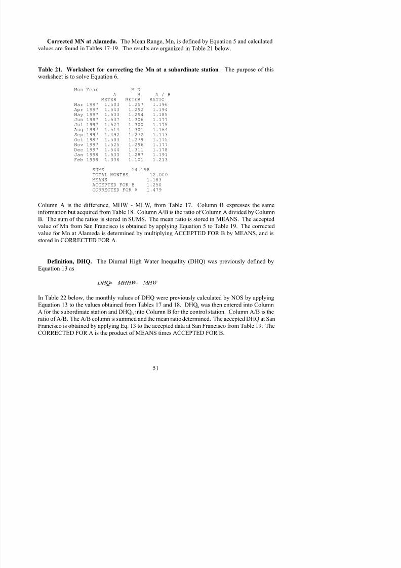
8/6/2019 Computational Techniques for Tidal Datums Handbook
http://slidepdf.com/reader/full/computational-techniques-for-tidal-datums-handbook 65/113
values are found in Tables 17-19. The results are organized in Table 21 below.
Table 21. Worksheet for correcting the Mn at a subordinate station. The purpose of this
worksheet is to solve Equation 6.
Mon Year M NA B A / B
METER METER RATIOMar 1997 1.503 1.257 1.196Apr 1997 1.543 1.292 1.194
May 1997 1.533 1.294 1.185Jun 1997 1.537 1.306 1.177Jul 1997 1.527 1.300 1.175Aug 1997 1.514 1.301 1.164Sep 1997 1.492 1.272 1.173Oct 1997 1.503 1.279 1.175Nov 1997 1.525 1.296 1.177Dec 1997 1.544 1.311 1.178Jan 1998 1.533 1.287 1.191Feb 1998 1.336 1.101 1.213
SUMS 14.198TOTAL MONTHS 12.000MEANS 1.183ACCEPTED FOR B 1.250CORRECTED FOR A 1.479
Column A is the difference, MHW - MLW, from Table 17. Column B expresses the same
information but acquired from Table 18. Column A/B is the ratio of Column A divided by Column
B. The sum of the ratios is stored in SUMS. The mean ratio is stored in MEANS. The accepted
value of Mn from San Francisco is obtained by applying Equation 5 to Table 19. The correctedvalue for Mn at Alameda is determined by multiplying ACCEPTED FOR B by MEANS, and is
stored in CORRECTED FOR A.
Definition, DHQ. The Diurnal High Water Inequality (DHQ) was previously defined by
Equation 13 as
DHQ MHHW MHW = −
In Table 22 below, the monthly values of DHQ were previously calculated by NOS by applying
Equation 13 to the values obtained from Tables 17 and 18. DHQA was then entered into Column
The mathematical form of the corrected DHQ is given by Eq. 15,

8/6/2019 Computational Techniques for Tidal Datums Handbook
http://slidepdf.com/reader/full/computational-techniques-for-tidal-datums-handbook 66/113
DLQ MLW MLLW = −
DHQ DHQ
N
DHQ I
DHQ I CORRECTED FOR A FOR B
A
B I
N
ACCEPTED (15).= ×
=
∑1
1
( )
( )
Table 22. Worksheet for calculating the corrected DHQ at a subordinate station. This
worksheet solves Eq. 15.
Mon Year DHQA B A / B
METER METER RATIOMar 1997 0.132 0.122 1.082Apr 1997 0.116 0.117 0.991May 1997 0.166 0.162 1.025Jun 1997 0.218 0.213 1.023Jul 1997 0.225 0.219 1.027Aug 1997 0.184 0.176 1.045Sep 1997 0.116 0.113 1.027Oct 1997 0.105 0.101 1.040Nov 1997 0.166 0.162 1.025Dec 1997 0.224 0.217 1.032Jan 1998 0.215 0.213 1.009Feb 1998 0.187 0.183 1.022
SUMS 12.348TOTAL MONTHS 12.000MEANS 1.029ACCEPTED FOR B 0.183
CORRECTED FOR A 0.188
Definition, DLQ. The Diurnal Low Water Inequality (DLQ) was previously defined by
Equation 14 as
In Table 23 below, DLQ values were previously calculated by NOS by applying Equation 13 to
values from Tables 17 and 18. DLQA and DLQB values were entered into Column A for the
subordinate and into Column B for the control. Column A/B is the ratio of A/B. The A/B column
is summed and the mean ratio determined. The accepted DLQ at San Francisco is obtained by
N
The mathematical form of the corrected DLQ is given by Equation 16,
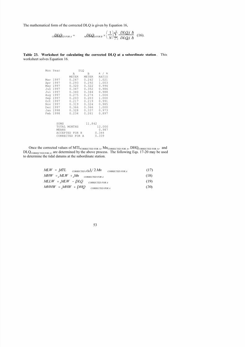
8/6/2019 Computational Techniques for Tidal Datums Handbook
http://slidepdf.com/reader/full/computational-techniques-for-tidal-datums-handbook 67/113
MLW MTL MnMHW MLW Mn
MLLW MLW DLQ
MHHW MHW DHQ
A CORRECTED FOR A CORRECTED FOR A
A A CORRECTED FOR A
A A CORRECTED FOR A
A A CORRECTED FOR A
= −= +
= −
= +
(17)(18)
(19)
1 2
20
/
. ( )
DLQ DLQ
N
DLQ I
DLQ I CORRECTED FOR A FOR B
A
B I
N
ACCEPTED (16).= ×
=
∑1
1
( )
( )
Table 23. Worksheet for calculating the corrected DLQ at a subordinate station. This
worksheet solves Equation 16.
Mon Year DLQA B A / BMETER METER RATIO
Mar 1997 0.247 0.242 1.021Apr 1997 0.293 0.292 1.003May 1997 0.320 0.322 0.994Jun 1997 0.347 0.352 0.986Jul 1997 0.340 0.344 0.988Aug 1997 0.275 0.274 1.004Sep 1997 0.203 0.203 1.000Oct 1997 0.217 0.219 0.991
Nov 1997 0.319 0.324 0.985Dec 1997 0.366 0.366 1.000Jan 1998 0.328 0.337 0.973Feb 1998 0.234 0.261 0.897
SUMS 11.842TOTAL MONTHS 12.000MEANS 0.987ACCEPTED FOR B 0.344CORRECTED FOR A 0.339
Once the corrected values of MTLCORRECTED FOR A, MnCORRECTED FOR A, DHQCORRECTED FOR A, and
DLQCORRECTED FOR A, are determined by the above process. The following Eqs. 17-20 may be used
to determine the tidal datums at the subordinate station.
In each of the four equations above, the values of MTLCORRECTED FOR A, MnCORRECTED FOR A,
DHQCORRECTED FOR A, and DLQCORRECTED FOR A, are entered from the appropriate CORRECTED FOR

8/6/2019 Computational Techniques for Tidal Datums Handbook
http://slidepdf.com/reader/full/computational-techniques-for-tidal-datums-handbook 68/113
MLW MTL Mn
MHW MLW Mn
MLLW MLW DLQ
MHHW MHW DHQ
A CORRECTED FOR A CORRECTED FOR A
A A CORRECTED FOR A
A A CORRECTED FOR A
A A CORRECTED FOR A
= − = − =
= + = + =
= − = − =
= + = + =
1 2 2 043 05 1479 1304
1304 1479 2 783
1304 0339 0965
2 783 0188 2971
/ . . ( . ) .
. . .
. . .
. . . .
A entry from Tables 20-23 above. MLWA, as derived from Eq. 17, is entered into Eqs. 18 and 19.
MHWA , as derived from Eq. 18, is entered into Eq. 20. For Alameda, the tidal datums are
Appendix 1. Part B, contains a composite example spreadsheet of the calculations described above.
4.3 Comparison of Simultaneous High and Low Waters (Tide by Tide Analysis)
The method of Comparison of Simultaneous High and Low Waters or, Tide by Tide Analysis
(TBYT), is used to compute datums form short-term stations. For instance, if the simultaneous
water level measurements at the subordinate and control stations exist for less than a month or if thedata series starts and ends in the middle of two consecutive months. The next three examples
illustrate this comparison method for three different types of tide. For each type, equivalent 19-year
datums are computed, in addition to lunitidal intervals. The example data may be downloaded from
the CO-OPS website. All data are in meters, referenced to station datum, and are on the Greenwich
time meridian. Referencing data series to Greenwich meridian is now the standard NOS practice.
When calculating time differences in the phase of tide between two stations, it is necessary to factor
in any differences in the time zone that the observations were recorded on. The present NOS
practice of operating all tide stations on GMT. Five days of simultaneous observations are used inthis example for illustration only. The estimated vertical error in the resultant datums for this series
length, extrapolating the curve from Figure 14, is expected to be greater than 0.04 m. At least one
month of data ensures closure on the significant monthly variations of the tide and provides a proper
number of values to get meaningful statistics from the comparisons. Using less than one month of
data is proper as long as the user realizes the higher uncertainties in the resulting datums.
The examples follow the procedural steps outlined in section 4.1.2. First, the data from thecontrol and subordinate stations are obtained and put into tabular form for comparisons.
Summations of the tides and their simultaneous differences are computed on the same tabular form.
Then, based on the summations and differences, a specific sequence of equations is used to form the
differences and ratios needed to compute the equivalent NDTE datums. Appendix 2 contains a
Data for this example may be downloaded from http://www.tidesandcurrents.noaa.gov/. Click
on the hyperlink for “Water Level Observations”, under the heading “Verified / Historical Water
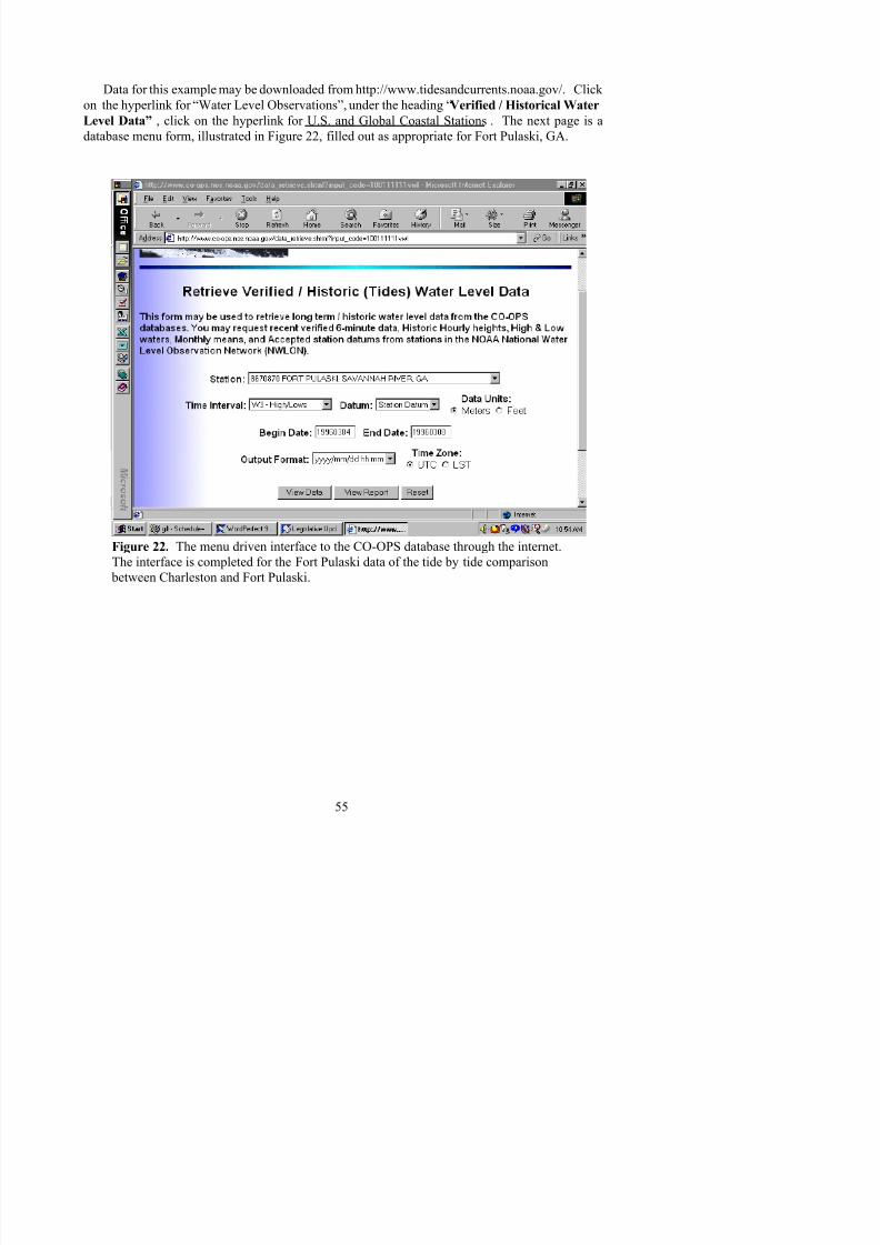
8/6/2019 Computational Techniques for Tidal Datums Handbook
http://slidepdf.com/reader/full/computational-techniques-for-tidal-datums-handbook 69/113
Figure 22. The menu driven interface to the CO-OPS database through the internet.
The interface is completed for the Fort Pulaski data of the tide by tide comparison
between Charleston and Fort Pulaski.
Level Data” , click on the hyperlink for U.S. and Global Coastal Stations . The next page is a
database menu form, illustrated in Figure 22, filled out as appropriate for Fort Pulaski, GA.
Note that in the scroll box under “Time Interval”, “W3 - High/Lows”, is selected. By clicking
on the button captioned, “View Data/View Report”, the database returns the information presented
i T bl 24 d Fi 23 Th ddi i l h l l l d d i Fi 28 i
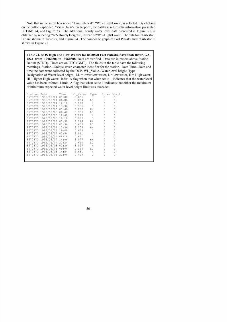
8/6/2019 Computational Techniques for Tidal Datums Handbook
http://slidepdf.com/reader/full/computational-techniques-for-tidal-datums-handbook 70/113
in Table 24, and Figure 23. The additional hourly water level data presented in Figure. 28, is
obtained by selecting “W2- Hourly Heights”, instead of “W3- High/Lows”. The data for Charleston,SC are shown in Table 25, and Figure 24. The composite graph of Fort Pulaski and Charleston is
shown in Figure 25.
Table 24. NOS High and Low Waters for 8670870 Fort Pulaski, Savannah River, GA,
USA from 19960304 to 19960308. Data are verified. Data are in meters above Station
Datum (STND). Times are on UTC (GMT). The fields in the table have the following
meanings. Station--Unique seven character identifier for the station. Date Time--Date andtime the data were collected by the DCP. WL_Value--Water level height. Type –
Designation of Water level height. LL = lower low water, L = low water, H = High water,
HH Higher High water. Infer--A flag when that when set to 1 indicates that the water level
value has been inferred. Limit--A flag that when set to 1 indicates that either the maximum
or minimum expected water level height limit was exceeded.
Station Date Time WL_Value Type Infer Limit
8670870 1996/03/04 00:00 3.066 H 0 08670870 1996/03/04 06:06 0.864 LL 0 08670870 1996/03/04 12:18 3.178 H 0 08670870 1996/03/04 18:36 0.956 L 0 08670870 1996/03/05 00:42 3.280 HH 0 08670870 1996/03/05 06:48 0.908 LL 0 08670870 1996/03/05 12:42 3.227 H 0 08670870 1996/03/05 19:18 0.973 L 0 08670870 1996/03/06 01:30 3.244 HH 0 08670870 1996/03/06 07:36 0.658 LL 0 0
8670870 1996/03/06 13:36 3.153 HH 0 08670870 1996/03/06 19:48 0.678 L 0 08670870 1996/03/07 01:54 3.061 H 0 08670870 1996/03/07 08:18 0.641 L 0 08670870 1996/03/07 14:06 3.077 HH 0 08670870 1996/03/07 20:24 0.610 LL 0 08670870 1996/03/08 02:36 3.027 H 0 08670870 1996/03/08 09:06 0.165 LL 0 08670870 1996/03/08 14:54 2.681 H 0 08670870 1996/03/08 21:06 0.429 L 0 0
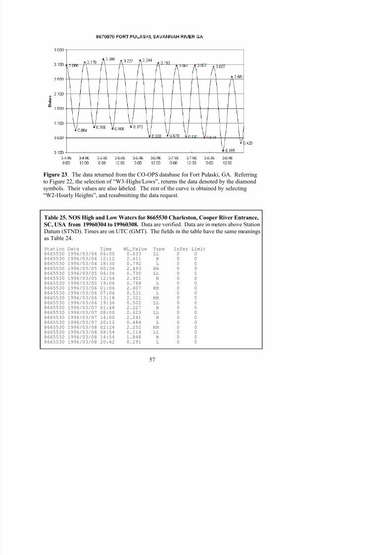
8/6/2019 Computational Techniques for Tidal Datums Handbook
http://slidepdf.com/reader/full/computational-techniques-for-tidal-datums-handbook 71/113
Table 25. NOS High and Low Waters for 8665530 Charleston, Cooper River Entrance,SC, USA from 19960304 to 19960308. Data are verified. Data are in meters above Station
Datum (STND). Times are on UTC (GMT). The fields in the table have the same meanings
as Table 24.
Station Date Time WL_Value Type Infer Limit8665530 1996/03/04 06:00 0.633 LL 0 08665530 1996/03/04 12:12 2.411 H 0 08665530 1996/03/04 18:30 0.792 L 0 08665530 1996/03/05 00:36 2.493 HH 0 0
8665530 1996/03/05 06:36 0.730 LL 0 08665530 1996/03/05 12:54 2.401 H 0 08665530 1996/03/05 19:06 0.768 L 0 08665530 1996/03/06 01:06 2.407 HH 0 08665530 1996/03/06 07:06 0.531 L 0 08665530 1996/03/06 13:18 2.321 HH 0 0
/ /
Figure 23. The data returned from the CO-OPS database for Fort Pulaski, GA. Referring
to Figure 22, the selection of “W3-Highs/Lows”, returns the data denoted by the diamond
symbols. Their values are also labeled. The rest of the curve is obtained by selecting
“W2-Hourly Heights”, and resubmitting the data request.
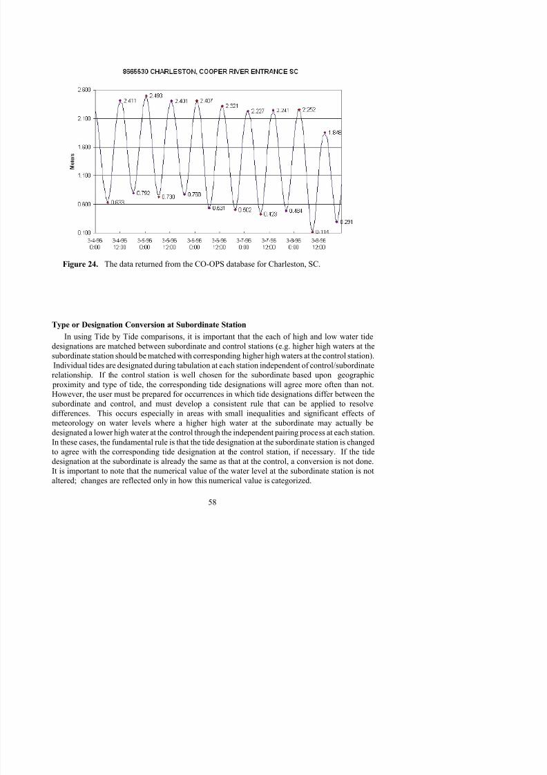
8/6/2019 Computational Techniques for Tidal Datums Handbook
http://slidepdf.com/reader/full/computational-techniques-for-tidal-datums-handbook 72/113
Figure 24. The data returned from the CO-OPS database for Charleston, SC.
Type or Designation Conversion at Subordinate Station
In using Tide by Tide comparisons, it is important that the each of high and low water tide
designations are matched between subordinate and control stations (e.g. higher high waters at the
subordinate station should be matched with corresponding higher high waters at the control station).
Individual tides are designated during tabulation at each station independent of control/subordinate
relationship. If the control station is well chosen for the subordinate based upon geographic
proximity and type of tide, the corresponding tide designations will agree more often than not.However, the user must be prepared for occurrences in which tide designations differ between the
subordinate and control, and must develop a consistent rule that can be applied to resolve
differences. This occurs especially in areas with small inequalities and significant effects of
l l l h hi h hi h h b di ll b
For example, in Figure 25, the first pair of water level values used in the analysis consist of
3.178 m at the subordinate and 2.411 m at the control. From Table 25, the value of 2.411 m is
categorized as an “H” From Table 24 at the subordinate 3 178 m is also categorized as an “H”
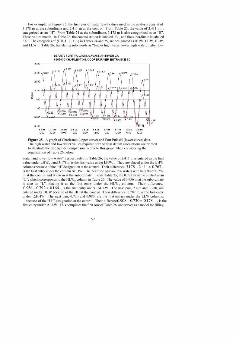
8/6/2019 Computational Techniques for Tidal Datums Handbook
http://slidepdf.com/reader/full/computational-techniques-for-tidal-datums-handbook 73/113
Figure 25. A graph of Charleston (upper curve) and Fort Pulaski (lower curve) data.
The high water and low water values required for the tidal datum calculations are printed
to illustrate the tide by tide comparison. Refer to this graph when considering the
organization of Table 26 below.
categorized as an H . From Table 24 at the subordinate, 3.178 m is also categorized as an H .
These values match. In Table 26, the control station is labeled “B”, and the subordinate is labeled“A”. The categories of {HH, H, L, LL} in Tables 24 and 25, are designated as HHW, LHW, HLW,
and LLW in Table 26; translating into words as “higher high water, lower high water, higher low
water, and lower low water”, respectively. In Table 26, the value of 2.411 m is entered as the first
value under LHWB , and 3.178 m is the first value under LHWA . They are placed under the LHW
columns because of the “H” designation at the control. Their difference, ,3178 2 411 0 767. . .− =is the first entry under the column )LHW. The next tide pair are low waters with heights of 0.792
m at the control and 0.956 m at the subordinate. From Table 25, the 0.792 m at the control is an
“L”, which corresponds to the HLWB column in Table 26. The value of 0.956 m at the subordinate
is also an “L” placing it as the first entry under the HLW column Their difference
in the rest of Table 26. So far, type conversion at the subordinate has not occurred. However,
continuing through this table example type conversion at the subordinate occurs a total of six times
as explained below
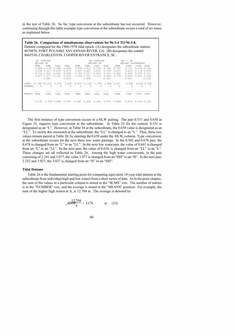
8/6/2019 Computational Techniques for Tidal Datums Handbook
http://slidepdf.com/reader/full/computational-techniques-for-tidal-datums-handbook 74/113
as explained below.
The first instance of type conversion occurs in a HLW pairing. The pair 0.531 and 0.658 in
Figure 25, requires type conversion at the subordinate. In Table 25 for the control, 0.531 is
designated as an “L”. However, in Table 24 at the subordinate, the 0.658 value is designated as an
“LL”. To rectify this mismatch at the subordinate, the “LL” is changed to an “L”. Thus, these twovalues remain paired in Table 26, by entering the 0.658 under the HLWA column. Type conversion
at the subordinate occurs for the next three low water pairings. In the 0.502 and 0.678 pair, the
0.678 is changed from an “L” to an “LL”. In the next low water pair, the value of 0.641 is changed
from an “L” to an “LL”. In the next pair, the value of 0.610, is changed from an “LL” to an “L”.
These changes are all reflected in Table 26. Among the high water conversions, in the pair
consisting of 2.241 and 3.077, the value 3.077 is changed from an “HH” to an “H”. In the next pair,
2.252 and 3.027, the 3.027 is changed from an “H” to an “HH”.
Tidal Datums
Table 26 is the fundamental starting point for computing equivalent 19-year tidal datums at the
subordinate from individual high and low waters from a short series of data. As in the prior chapter,
h f h l i i l l i d i h “SUMS” Th b f i
Table 26. Comparison of simultaneous observations for 96-3-4 TO 96-3-8.
Datums computed for the 1960-1978 tidal epoch. (A) designates the subordinate station,
8670870, FORT PULASKI, SAVANNAH RIVER, GA. (B) designates the control
8665530, CHARLESTON, COOPER RIVER ENTRANCE, SC.
(A) STATION (B) STATION (A) - (B)HEIGHT OF HEIGHT OF HEIGHT DIFFERENCEHHWA LHWA LLWA HLWA HHWB LHWB LLWB HLWB )HHW )LHW )LLW )HLW
3.280 3.178 0.908 0.956 2.493 2.411 0.730 0.792 0.787 0.767 0.178 0.1643.244 3.227 0.678 0.973 2.407 2.401 0.502 0.768 0.837 0.826 0.176 0.2053.153 3.061 0.641 0.658 2.321 2.227 0.423 0.531 0.832 0.834 0.218 0.1273.027 3.077 0.165 0.610 2.252 2.241 0.114 0.484 0.775 0.836 0.051 0.126
2.681 0.429 1.848 0.291 0.833 0.138
SUMS: 12.704 15.224 2.392 3.626 9.473 11.128 1.769 2.866 3.231 4.096 0.623 0.760NUMBER: 4 5 4 5 4 5 4 5 4 5 4 5
———— ———— ——— ———— ———— ———— ———— ———— ————— ————— ————— ————— MEANS: HHWA LHWA LLWA HLWA HHWB LHWB LLWB HLWB )HHW )LHW )LLW )HLW
3.176 3.045 0.598 0.725 2.368 2.226 0.442 0.573 0.808 0.819 0.156 0.152
Similar averages are computed as shown in Table 26 for , , for the LHW A LLW A HLW A
subordinate station and for , , , for the control station. In addition, HHW B LHW B LLW B HLW B
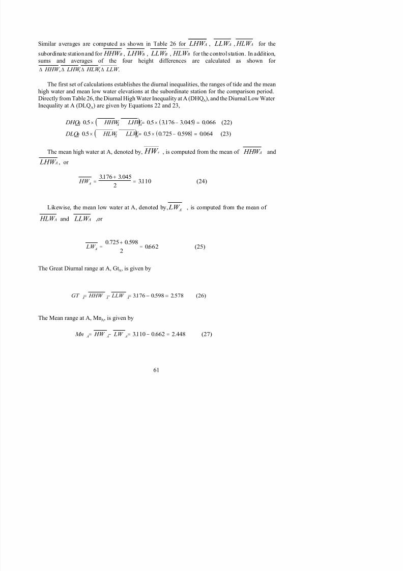
8/6/2019 Computational Techniques for Tidal Datums Handbook
http://slidepdf.com/reader/full/computational-techniques-for-tidal-datums-handbook 75/113
GT HHW LLW A A A= − = − =3176 0 598 2 578. . . (26)
( ) ( )
( ) ( )
DHQ HHW LHW
DLQ HLW LLW
A A A
A A A
= × − = × − =
= × − = × − =
05 05 3176 3 045 0 066
05 05 0 725 0598 0
. . . . .
. . . . .
(22)
064 (23)
HW A =+
=3176 3 045
23110
. .. (24)
LW A =+
=0 725 0 598
20662
. .. (25)
sums and averages of the four height differences are calculated as shown for
.∆ ∆ ∆ ∆ HHW LHW HLW LLW , , ,
The first set of calculations establishes the diurnal inequalities, the ranges of tide and the mean
high water and mean low water elevations at the subordinate station for the comparison period.
Directly from Table 26, the Diurnal High Water Inequality at A (DHQA), and the Diurnal Low Water
Inequality at A (DLQA) are given by Equations 22 and 23,
The mean high water at A, denoted by, , is computed from the mean of and HW A HHW A
, or LHW A
Likewise, the mean low water at A, denoted by, , is computed from the mean of LW A
and ,or HLW A LLW A
The Great Diurnal range at A, GtA, is given by
( ) ( )DTL HHW LLW× + × +05 05 3176 0598 1887 (28)
The Diurnal Tide Level at A, DTLA, is given by
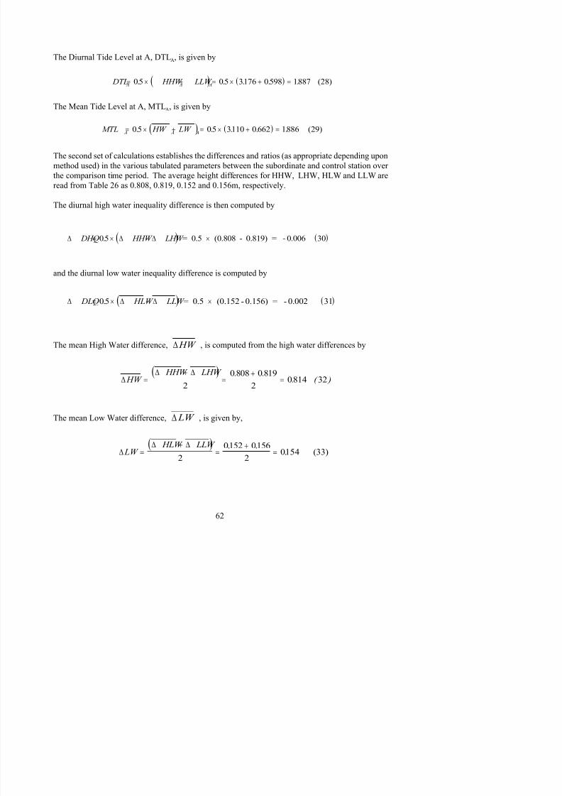
8/6/2019 Computational Techniques for Tidal Datums Handbook
http://slidepdf.com/reader/full/computational-techniques-for-tidal-datums-handbook 76/113
( ) ( ) DTL HHW LLW A A A= × + = × + =05 05 3176 0598 1887. . . . . (28)
( ) ( )MTL HW LW A A A= × + = × + =05 05 3110 0 662 1886. . . . . (29)
( )∆
∆ ∆ HW
HHW LHW . .. ( )=
+=
+=
2
0 808 0 819
20814 32
The Mean Tide Level at A, MTLA, is given by
The second set of calculations establishes the differences and ratios (as appropriate depending upon
method used) in the various tabulated parameters between the subordinate and control station over the comparison time period. The average height differences for HHW, LHW, HLW and LLW are
read from Table 26 as 0.808, 0.819, 0.152 and 0.156m, respectively.
The diurnal high water inequality difference is then computed by
( ) ( )∆ ∆ ∆ DHQ HHW LHW = × − ×05 30. = 0.5 (0.808 - 0.819) = - 0.006
and the diurnal low water inequality difference is computed by
( ) ( )∆ ∆ ∆ DLQ HLW LLW = × − ×05 31. = 0.5 (0.152 - 0.156) = - 0.002
The mean High Water difference, , is computed from the high water differences by∆ HW
The mean Low Water difference, , is given by,∆ LW
∆ ∆ ∆M HW LW 0814 0154 0 660 (34)
The Mean Range difference, )Mn, is given by,

8/6/2019 Computational Techniques for Tidal Datums Handbook
http://slidepdf.com/reader/full/computational-techniques-for-tidal-datums-handbook 77/113
( ) ( )∆ ∆ ∆ DTL HHW LLW = × + = × + =0 5 0 5 0 808 0156 0 482. . . . . (35)
( ) ( )∆ ∆ ∆MTL HW LW = × + = × + =0 5 05 0 814 0154 0 484. . . . . (36)
MnMn
Mn Mn
DHQ DHQ DHQ DHQ
DLQDLQ
DLQ DLQ
RATIO
A
A
RATIO A
A
RATIO
A
A
=−
= =
=−
=− −
=
=−
=− −
=
∆
∆
∆
2.449
2.449 - 0.660(38)
(39)
(40)
1369
00660 066 0 006
0917
0064
0 064 0 0020970
.
.. ( . )
.
.
. ( . ).
Gt Gt Gt Gt RATIO
A
A
=−
=−
=∆
25782 578 0 652
1339.. .
. (41)
∆ ∆ ∆Mn HW LW = − = − =0814 0154 0 660. . . (34)
∆ ∆ ∆Gt HHW LLW = − = − =0808 0156 0 652. . . (37)
The Diurnal Tide Level difference, )DTL, is given by,
The Mean Tide Level difference, )MTL, is given by,
The Great Diurnal range difference, )Gt, is given by,
The Mean Range Ratio, MnRATIO , the Diurnal High Water Inequality Ratio, DHQRATIO, and the
Diurnal Low Water Inequality Ratio, DLQRATIO, are given by
The Great Diurnal Ratio, GtRATIO , is given by
Table 5 presents the accepted 19 year tidal datums for Charleston the control station for this
MTL MTL MTL= + ∆
The MTLCORRECTED FOR A is given by,
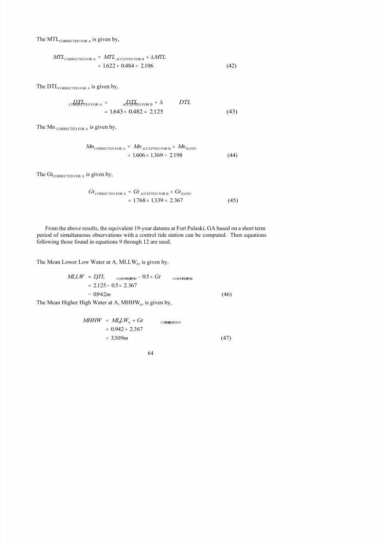
8/6/2019 Computational Techniques for Tidal Datums Handbook
http://slidepdf.com/reader/full/computational-techniques-for-tidal-datums-handbook 78/113
Mn Mn MnCORRECTED ACCEPTED RATIOFOR A FOR B
(44)
= ×
= × =1606 1369 2198. . .
MTL MTL MTLCORRECTED ACCEPTEDFOR A FOR B
(42)
= +
= + =
∆
1622 0 484 2106. . .
DTL DTL DTLCORRECTED ACCEPTEDFOR A FOR B
(43)
= +
= + =
∆
1643 0 482 2125. . .
Gt Gt Gt CORRECTED ACCEPTED RATIOFOR A FOR B
(45)
= ×
= × =1768 1339 2 367. . .
MLLW DTL Gt
m
A CORRECTED CORRECTED= − ×
= − ×
=
FOR A FOR A
(46)
05
2125 05 2 367
0942
.
. . .
The DTLCORRECTED FOR A is given by,
The Mn CORRECTED FOR A is given by,
The GtCORRECTED FOR A is given by,
From the above results, the equivalent 19-year datums at Fort Pulaski, GA based on a short term
period of simultaneous observations with a control tide station can be computed. Then equations
following those found in equations 9 through 12 are used.
The Mean Lower Low Water at A, MLLWA, is given by,
MLW MTL M05
The Mean Low Water at A, MLWA, is given by,

8/6/2019 Computational Techniques for Tidal Datums Handbook
http://slidepdf.com/reader/full/computational-techniques-for-tidal-datums-handbook 79/113
MLW MTL Mn
m
A CORRECTED CORRECTED
= − ×
= − ×
=
FOR A FOR A
(48)
05
2106 05 2198
1007
.
. . .
.
MHW MLW Mn
m
A CORRECTED= +
= +=
A FOR A
(49)
1007 2 198
3205
. .
.
The Mean High Water at A, MHWA, is given by,
Lunitidal Intervals
Lunitidal Intervals can provide a measure of the average difference in time of tide between two
locations. When sufficient data are available and monthly mean values are computed for a station,
the monthly Greenwich Mean High Water Interval (HWI) and Greenwich Mean Low Water Interval
(LWI) are among the means routinely computed by NOS for stations with semidiurnal and mixed tide
types. These stations usually have a one-to-one correspondence between the tides (high and low
waters) and the transits of the moon relative to the Greenwich meridian. As stated earlier, the
Greenwich Intervals represent the mean difference in time between the upper and lower passage of
the moon over the Greenwich Meridian and the following high and low tides observed at a station.
The monthly mean HWI and LWI can be used to compute the average time difference in the phase
of tide between different locations by subtracting one from the other. When only a short series of
data is available, as in the present example, the time differences between individual corresponding
tides are computed, and then the means of these differences are computed to provide this information.
In this section we compute the equivalent 19-year Greenwich High Water Interval (HWI) and
Low Water Interval (LWI) at the subordinate station. To compute the tidal datums above, the notion
of time was handled implicitly, simply by organizing the pairs of high or low values sequentially in
Table 26. Here, the time aspect is treated explicitly. Table 27, like Table 26, is based upon the
information presented in Tables 24 and 25. Table 27 includes the water level heights for stations A
and B to show correct matching, but the elevations are not used to compute the HWI and LWI. The
first pair of corresponding high waters have heights of 3.178 m and 2.411 m(Figure 34). These arethe first entries under the HW column of stations A and B, respectively. The time associated with
3.178 is 1996/03/04 12:18 GMT (Table 27), and the time associated with 2.411 is 1996/03/04 12:12
GMT. These times have been converted from hours: minutes format to decimal hours in Table 27.
Th diff 12 3 12 2 0 1 i h fi d h HW H Ti Diff l Th
The mean high water time difference is 0.12 hours, and the mean low water time difference is
0.26 hours (Table 27). From Table 5, the accepted HWI at Station B is 0.35 hours, and the accepted
LWI interval is 6.57 hours.
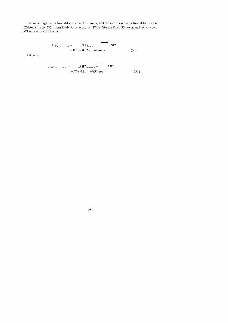
8/6/2019 Computational Techniques for Tidal Datums Handbook
http://slidepdf.com/reader/full/computational-techniques-for-tidal-datums-handbook 80/113
HWI HWI HWI
hours
CORRECTED ACCEPTEDFOR A FOR B
(50)
= +
= + =0 35 012 047. . .
LWI LWI LWI hours
CORRECTED ACCEPTEDFOR A FOR B
(51)= += + =657 0 26 683. . .
Likewise,
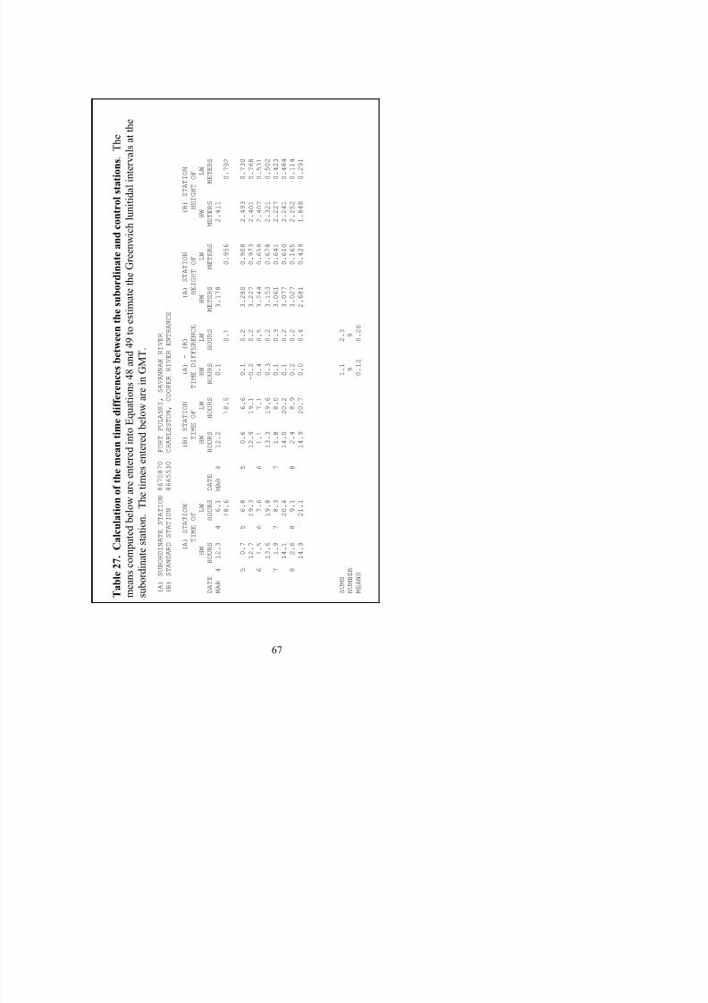
8/6/2019 Computational Techniques for Tidal Datums Handbook
http://slidepdf.com/reader/full/computational-techniques-for-tidal-datums-handbook 81/113
C a l c u l a t i o n o f t h e m e a n t i m e d i f f e r e n c e s b e t w e e n t h e s
u b o r d i n a t e a n d c o n t r o l s t a t i o n s . T h e
u t e d b e l o w a r e e n t e r e d i n t o E q u a t i o n s 4 8 a n d 4 9 t o e s t i m
a t e t h e G r e e n w i c h l u n
i t i d a l i n t e r v a l s a t t h e
s t a t i o n . T h e
t i m e s e n t e r e d b e l o w a r e i n G M T .
N A T E S T A T I O N
8 6 7 0 8 7 0
F O R T P U L A S K I ,
S A V A N N A H R I V E R
D S T A T I O N
8 6 6 5 5 3 0
C H A R L E S T O N , C
O O P E R R I V E R E N T R A N C E
A ) S T A T I O N
( B ) S T A T I O N
( A ) -
( B )
( A ) S T A T I O N
( B ) S T A T I O N
T I M E O F
T I M E O F
T I M E D I F F E R E N C E
H E I G H T O F
H E I G H T O F
L W
H W
L W
H W
L W
H W
L W
H W
L W
S
H O U R S
D A T E
H O U R S
H O U R S
H O U R S
H O U R S
M E
T E R S
M E T E R S
M E T E R S
M E T E R S
3
4
6 . 1
M A R
4
1 2 . 2
0 . 1
3
. 1 7 8
2 . 4 1 1
1 8 . 6
1 8 . 5
0 . 1
0 . 9 5 6
0 . 7 9 2
7
5
6 . 8
5
0 . 6
6 . 6
0 . 1
0 . 2
3
. 2 8 0
0 . 9 0 8
2 . 4 9 3
0 . 7 3 0
7
1 9 . 3
1 2 . 9
1 9 . 1
- 0 . 2
0 . 2
3
. 2 2 7
0 . 9 7 3
2 . 4 0 1
0 . 7 6 8
5
6
7 . 6
6
1 . 1
7 . 1
0 . 4
0 . 5
3
. 2 4 4
0 . 6 5 8
2 . 4 0 7
0 . 5 3 1
6
1 9 . 8
1 3 . 3
1 9 . 6
0 . 3
0 . 2
3
. 1 5 3
0 . 6 7 8
2 . 3 2 1
0 . 5 0 2
9
7
8 . 3
7
1 . 8
8 . 0
0 . 1
0 . 3
3
. 0 6 1
0 . 6 4 1
2 . 2 2 7
0 . 4 2 3
1
2 0 . 4
1 4 . 0
2 0 . 2
0 . 1
0 . 2
3
. 0 7 7
0 . 6 1 0
2 . 2 4 1
0 . 4 8 4
6
8
9 . 1
8
2 . 4
8 . 9
0 . 2
0 . 2
3
. 0 2 7
0 . 1 6 5
2 . 2 5 2
0 . 1 1 4
9
2 1 . 1
1 4 . 9
2 0 . 7
0 . 0
0 . 4
2
. 6 8 1
0 . 4 2 9
1 . 8 4 8
0 . 2 9 1
1 . 1
2 . 3
9
9
0 . 1 2
0 . 2 6
4.3.2 Modified Range Ratio - Diurnal Tides
A comparison of Simultaneous High and Low Waters, also referred to as a Tide by Tide
Comparison is used to compute short term datums if the simultaneous water level measurements at
8/6/2019 Computational Techniques for Tidal Datums Handbook
http://slidepdf.com/reader/full/computational-techniques-for-tidal-datums-handbook 82/113
the subordinate and control exist for less than a month. Consider Figure 26, which illustrates the period of time from March 10 through March 16, 1996 at Panama City Beach and Pensacola, FL.
The moon was in the tropics during this time period, producing a clean example of simultaneous
diurnal tides at the subordinate and control. The data downloaded from the CO-OPS website are
presented in Tables 28 and 29.
In Figure 26, the values of the high and low waters are plotted to facilitate understanding. The
first step is to track the high and low waters correctly. Generally, this can be done by allowing a day
to elapse to make sure that a peak and trough cycle have been resolved by each time series. Hence,the analysis begins with the trough of March 11, 1996, and records each high water and low water
pair thereafter.
In Table 30, Panama City Beach, the subordinate station, is designated A, and Pensacola, the
control station, is B. The left pair of columns represents the height of the high and low waters at
Panama City Beach. Units are meters. The middle pair represent the height of the high and low
waters at Pensacola. The right pair of columns represent the difference between the high waters at
A and B, and the difference between the low waters at A and B. For example the first entry in the
right pair is in the LW column, and is simply the low water at A minus the low water at B, or 7.843 -
2.271 = 5.572. For the HW field, the difference is the high water at A minus the high water at B, or
8.167 - 2.578 = 5.589. Focusing now on the leftmost pair, the sum of the high waters at A is 42.253
from 5 observations, hence the mean HHW ( )is 8.451. Likewise, the mean lower low water, HHW A
( ) is 8.014. The higher high water at B, ( ) , is 2.806. The lower low water at B, ( )is LLW A HHW B LLW B
2.383. The mean difference of the high waters between A and B,( ) is 5.645. The mean∆ HHW
difference of the low waters ( ) is 5.632.∆ LLW
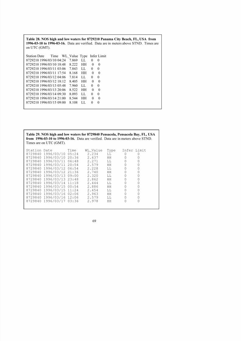
8/6/2019 Computational Techniques for Tidal Datums Handbook
http://slidepdf.com/reader/full/computational-techniques-for-tidal-datums-handbook 83/113
Table 28. NOS high and low waters for 8729210 Panama City Beach, FL, USA from1996-03-10 to 1996-03-16. Data are verified. Data are in meters above STND. Times are
on UTC (GMT).
Station Date Time WL_Value Type Infer Limit
8729210 1996/03/10 04:24 7.869 LL 0 0
8729210 1996/03/10 18:48 8.222 HH 0 0
8729210 1996/03/11 03:06 7.843 LL 0 0
8729210 1996/03/11 17:54 8.168 HH 0 0
8729210 1996/03/12 04:06 7.814 LL 0 0
8729210 1996/03/12 18:12 8.405 HH 0 0
8729210 1996/03/13 05:48 7.960 LL 0 0
8729210 1996/03/13 20:06 8.522 HH 0 0
8729210 1996/03/14 09:30 8.093 LL 0 0
8729210 1996/03/14 21:00 8.544 HH 0 0
8729210 1996/03/15 09:00 8.108 LL 0 0
Table 29. NOS high and low waters for 8729840 Pensacola, Pensacola Bay, FL, USA
from 1996-03-10 to 1996-03-16. Data are verified. Data are in meters above STND.
Times are on UTC (GMT).
Station Date Time WL_Value Type Infer Limit8729840 1996/03/10 05:24 2.234 LL 0 08729840 1996/03/10 20:36 2.637 HH 0 08729840 1996/03/11 06:48 2.271 LL 0 08729840 1996/03/11 20:54 2.579 HH 0 0
8729840 1996/03/12 06:54 2.228 LL 0 08729840 1996/03/12 21:36 2.740 HH 0 08729840 1996/03/13 09:00 2.320 LL 0 08729840 1996/03/13 23:48 2.862 HH 0 08729840 1996/03/14 11:18 2.444 LL 0 0
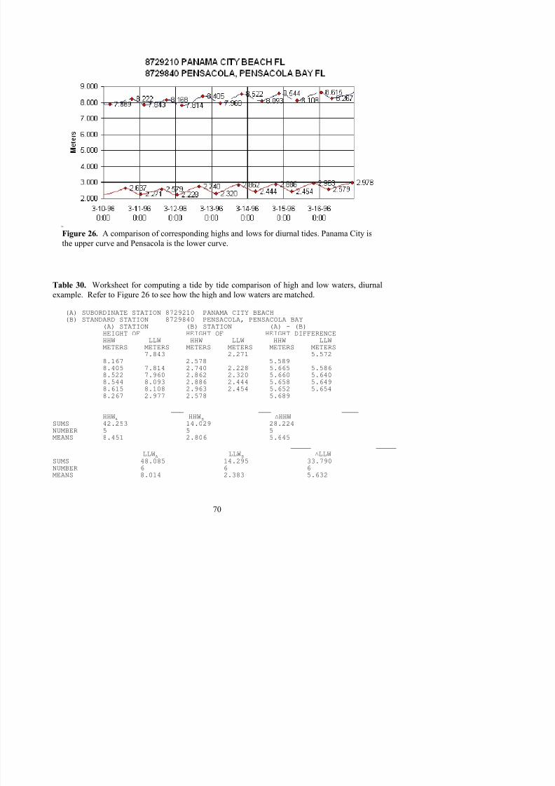
8/6/2019 Computational Techniques for Tidal Datums Handbook
http://slidepdf.com/reader/full/computational-techniques-for-tidal-datums-handbook 84/113
Figure 26. A comparison of corresponding highs and lows for diurnal tides. Panama City is
the upper curve and Pensacola is the lower curve.
Table 30. Worksheet for computing a tide by tide comparison of high and low waters, diurnal
example. Refer to Figure 26 to see how the high and low waters are matched.
(A) SUBORDINATE STATION 8729210 PANAMA CITY BEACH(B) STANDARD STATION 8729840 PENSACOLA, PENSACOLA BAY(A) STATION (B) STATION (A) - (B)HEIGHT OF HEIGHT OF HEIGHT DIFFERENCEHHW LLW HHW LLW HHW LLWMETERS METERS METERS METERS METERS METERS
7.843 2.271 5.5728.167 2.578 5.5898.405 7.814 2.740 2.228 5.665 5.5868.522 7.960 2.862 2.320 5.660 5.6408.544 8.093 2.886 2.444 5.658 5.649
8.615 8.108 2.963 2.454 5.652 5.6548.267 2.977 2.578 5.689
___ ___ ____HHWA HHWB )HHW
SUMS 42.253 14.029 28.224
Tidal Datums
Recalling the definition of Gt is MHHW - MLLW, the Gt at A for this time period, GtA, is formed
by Equation 52,

8/6/2019 Computational Techniques for Tidal Datums Handbook
http://slidepdf.com/reader/full/computational-techniques-for-tidal-datums-handbook 85/113
Gt MHHW MLLW ACCEPTEDFORB = − = − =2 911 2 524 0 387. . . (57)
Gt HHW LLW A A A= − = − =8 451 8 014 0 437. . . (52)
( ) ( ) DTL HHW LLW A A A= × + = × + =05 05 8 451 8014 8 232. . . . . (53)
∆ ∆ ∆Gt HHW LLW = − = 5.645- 5.632 = 0.013 (54)
Gt Gt
Gt Gt RATIO
A
A
=−
=−
=∆
0437
0 437 0 0131031
.
. .. (55)
( )( )
∆ ∆ ∆ DTL HHW LLW A A= × +× +
0505 5645 5632
.. . .= = 5.638 (56)
Similarly, the DTL at A may be defined as Equation 53,
The average Gt difference, is given by Equation 54,
The Gt ratio, is defined by Eq. 55,
The DTL difference, is defined by Eq. 56,
Recalling from Table 12, the accepted 19 year values of MHHW and MLLW for Pensacola, are 2.911
and 2.524, respectively, the accepted Gt and DTL values may be determined as,
Gt Gt Gt CORRECTED ACCEPTED RATIOFOR A FOR B= ×
The Gt, corrected for A, is given by Equation 59,
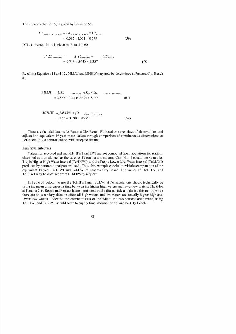
8/6/2019 Computational Techniques for Tidal Datums Handbook
http://slidepdf.com/reader/full/computational-techniques-for-tidal-datums-handbook 86/113
(59)= × =0 387 1031 0 399. . .
DTL DTL DTLCORRECTEDFORA ACCEPTEDFORB DIFFERENCE = +
= + = (60)2 719 5638 8 357. . .
MHHW MLLW Gt A A CORRECTEDFORA= +
= + = (62)8156 0 399 8555. . .
MLLW DTL Gt A CORRECTEDFORA CORRECTEDFORA= − ×
= − × =
05
8 357 05 0 399 8156
.
. . ( . ) . (61)
DTL, corrected for A is given by Equation 60,
Recalling Equations 11 and 12 , MLLW and MHHW may now be determined at Panama City Beach
as,
These are the tidal datums for Panama City Beach, FL based on seven days of observations and
adjusted to equivalent 19-year mean values through comparison of simultaneous observations at
Pensacola, FL, a control station with accepted datums.
Lunitidal Intervals
Values for accepted and monthly HWI and LWI are not computed from tabulations for stations
classified as diurnal, such as the case for Pensacola and panama City, FL. Instead, the values for
Tropic Higher High Water Interval (TcHHWI), and the Tropic Lower Low Water Interval (TcLLWI)
produced by harmonic analyses are used. Thus, this example concludes with the computation of theequivalent 19-year TcHHWI and TcLLWI at Panama City Beach. The values of TcHHWI and
TcLLWI may be obtained from CO-OPS by request.
bl 31 b l h d l h ld h i ll b
TcHHWI TcHHWI HWI
h
CORRECTED ACCEPTEDFOR A FOR B
(63)
≈ +
395 300 6 95
8/6/2019 Computational Techniques for Tidal Datums Handbook
http://slidepdf.com/reader/full/computational-techniques-for-tidal-datums-handbook 87/113
hours (63)≈ + =395 300 6 95. . .
TcLLWI TcLLWI LWI
hours
CORRECTED ACCEPTEDFOR A FOR B
(64)
≈ +
≈ + =1527 300 18 27. . .
Likewise,
These tropic intervals are used to estimate average time differences in the tide between diurnal
stations, however they are most accurate during tropic tides (maximum north and south declination
of the moon each month ) and typically are inaccurate during times of equatorial tides (when the
moon is on the equator each month).
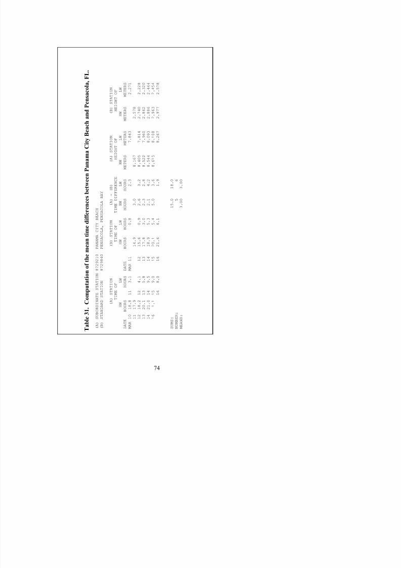
8/6/2019 Computational Techniques for Tidal Datums Handbook
http://slidepdf.com/reader/full/computational-techniques-for-tidal-datums-handbook 88/113
. C o m p u t a
t i o n o f t h e m e a n t i m e
d i f f e r e n c e s b e t w e e n
P a n a m a C i t y B e a c h a n d P e n s a c o l a ,
F L .
R D I N A T E S T A T
I O N
8 7 2 9 2 1 0
P A N A M A C I T Y B E A C H
D A R D S T A T I O N
8 7 2 9 8 4 0
P E N S A C O L A , P E N S A C O L A B A Y
( A ) S T A T I O
N
( B ) S T A T I O N
( A ) -
( B )
( A ) S T A T I O N
( B ) S T A T I O N
T I M E O F
T I M E O F
T I M E D I F F E R E N C E
H E I G H T O F
H E I G H T O F
H W
L
W
H W
L W
H W
L W
H W
L W
H W
L W
O U R S
H O U
R S
D A T E
H O U R S
H O U R S
H O U R S
H O U R S
M E T E R S
M E T E R S
M
E T E R S
M E T E R S
1 8 . 8
1 1
3
. 1
M A R
1 1
0 . 8
2 . 3
7 . 8 4 3
2 . 2 7 1
1 7 . 9
1 4 . 9
3 . 0
8 . 1 6 7
2 . 5 7 8
1 8 . 2
1 2
4
. 1
1 2
1 5 . 6
0 . 9
2 . 6
3 . 2
8 . 4 0 5
7 . 8 1 4
2 . 7 4 0
2 . 2 2 8
2 0 . 1
1 3
5
. 8
1 3
1 7 . 8
3 . 0
2 . 3
2 . 8
8 . 5 2 2
7 . 9 6 0
2 . 8 6 2
2 . 3 2 0
2 1 . 0
1 4
9
. 5
1 4
1 8 . 9
5 . 3
2 . 1
4 . 2
8 . 5 4 4
8 . 0 9 3
2 . 8 8 6
2 . 4 4 4
1 . 1
1 5
9
. 0
1 5
2 0 . 1
5 . 4
5 . 0
3 . 6
8 . 6 1 5
8 . 1 0 8
2 . 9 6 3
2 . 4 5 4
1 6
8
. 0
1 6
2 1 . 6
6 . 1
1 . 9
8 . 2 6 7
2 . 9 7 7
2 . 5 7 8
1 5 . 0
1 8 . 0
5
6
3 . 0 0
3 . 0 0
4.3.3 Standard Method - Mixed Tides
This section presents a mixed tides tide by tide case between Alameda and San Francisco, CA
(Tables 32 and 33). Figures 27-29 show a short series of observations from Alameda, San Francisco,
and a composite graph of the two The analysis is different from the purely diurnal case because it

8/6/2019 Computational Techniques for Tidal Datums Handbook
http://slidepdf.com/reader/full/computational-techniques-for-tidal-datums-handbook 89/113
Table 32. NOS high and low waters for 9414750 Alameda, San Francisco Bay, CA,
USA from 1997-03-01 to 1997-03-07. Data are verified. Data are in meters above
STND. Times are on UTC (GMT).
Station Date Time WL_Value Type Infer Limit9414750 1997/03/01 00:12 2.332 H 0 09414750 1997/03/01 05:36 1.655 L 0 0
9414750 1997/03/01 12:06 2.748 HH 0 09414750 1997/03/01 19:06 1.306 LL 0 09414750 1997/03/02 01:42 2.250 H 0 09414750 1997/03/02 06:24 1.744 L 0 09414750 1997/03/02 13:06 2.815 HH 0 09414750 1997/03/02 20:12 1.214 LL 0 09414750 1997/03/03 03:06 2.304 H 0 09414750 1997/03/03 07:48 1.784 L 0 09414750 1997/03/03 14:06 2.768 HH 0 0
9414750 1997/03/03 21:24 1.039 LL 0 09414750 1997/03/04 04:12 2.352 H 0 09414750 1997/03/04 09:06 1.725 L 0 09414750 1997/03/04 15:18 2.814 HH 0 09414750 1997/03/04 22:18 0.848 LL 0 09414750 1997/03/05 05:12 2.468 H 0 09414750 1997/03/05 10:06 1.642 L 0 09414750 1997/03/05 16:30 2.940 HH 0 09414750 1997/03/05 23:06 0.729 LL 0 0
9414750 1997/03/06 06:06 2.641 H 0 09414750 1997/03/06 11:12 1.527 L 0 09414750 1997/03/06 17:30 3.077 HH 0 09414750 1997/03/07 00:00 0.705 LL 0 09414750 1997/03/07 06:48 2.784 H 0 0
/ /
and a composite graph of the two. The analysis is different from the purely diurnal case because itinvolves the tabulation of the full set of observations of Higher High Water (HHW), Lower High
Water (LHW), Lower Low Water (LLW), and Higher Low Water (HLW) at both stations.
Tabulating the means from Figure 38 requires a more complex table structure (Table 34). A full
example spreadsheet showing all aspects of this comparison is found in Appendix 2.
Table 33. NOS high and low waters for 9414290 San Francisco, San Francisco Bay,
CA, USA from 1997-03-01 to 1997-03-07. Data are verified. Data are in meters above
STND Times are on UTC (GMT)
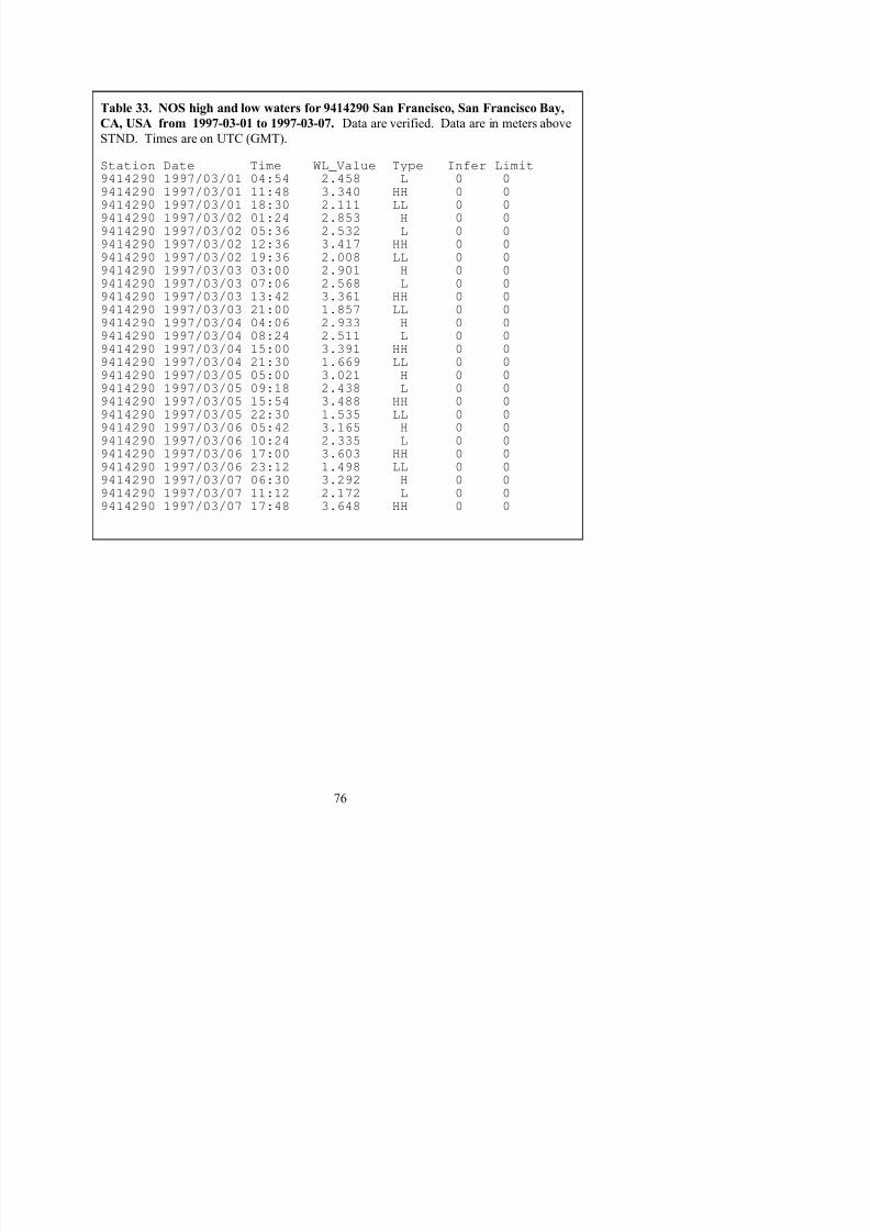
8/6/2019 Computational Techniques for Tidal Datums Handbook
http://slidepdf.com/reader/full/computational-techniques-for-tidal-datums-handbook 90/113
STND. Times are on UTC (GMT).
Station Date Time WL_Value Type Infer Limit9414290 1997/03/01 04:54 2.458 L 0 09414290 1997/03/01 11:48 3.340 HH 0 09414290 1997/03/01 18:30 2.111 LL 0 09414290 1997/03/02 01:24 2.853 H 0 09414290 1997/03/02 05:36 2.532 L 0 09414290 1997/03/02 12:36 3.417 HH 0 0
9414290 1997/03/02 19:36 2.008 LL 0 09414290 1997/03/03 03:00 2.901 H 0 09414290 1997/03/03 07:06 2.568 L 0 09414290 1997/03/03 13:42 3.361 HH 0 09414290 1997/03/03 21:00 1.857 LL 0 09414290 1997/03/04 04:06 2.933 H 0 09414290 1997/03/04 08:24 2.511 L 0 09414290 1997/03/04 15:00 3.391 HH 0 09414290 1997/03/04 21:30 1.669 LL 0 0
9414290 1997/03/05 05:00 3.021 H 0 09414290 1997/03/05 09:18 2.438 L 0 09414290 1997/03/05 15:54 3.488 HH 0 09414290 1997/03/05 22:30 1.535 LL 0 09414290 1997/03/06 05:42 3.165 H 0 09414290 1997/03/06 10:24 2.335 L 0 09414290 1997/03/06 17:00 3.603 HH 0 09414290 1997/03/06 23:12 1.498 LL 0 09414290 1997/03/07 06:30 3.292 H 0 0
9414290 1997/03/07 11:12 2.172 L 0 09414290 1997/03/07 17:48 3.648 HH 0 0
Table 34. Worksheet for calculating a tide by tide analysis for a mixed tide case.
COMPARISON OF SIMULTANEOUS OBSERVATIONS FOR 97 3 1 TO 97 3 7(A) SUBORDINATE STATION 9414750 ALAMEDA, SAN FRANCISCO BAY(B) STANDARD STATION 9414290 SAN FRANCISCO, SAN FRANCISCO BAY
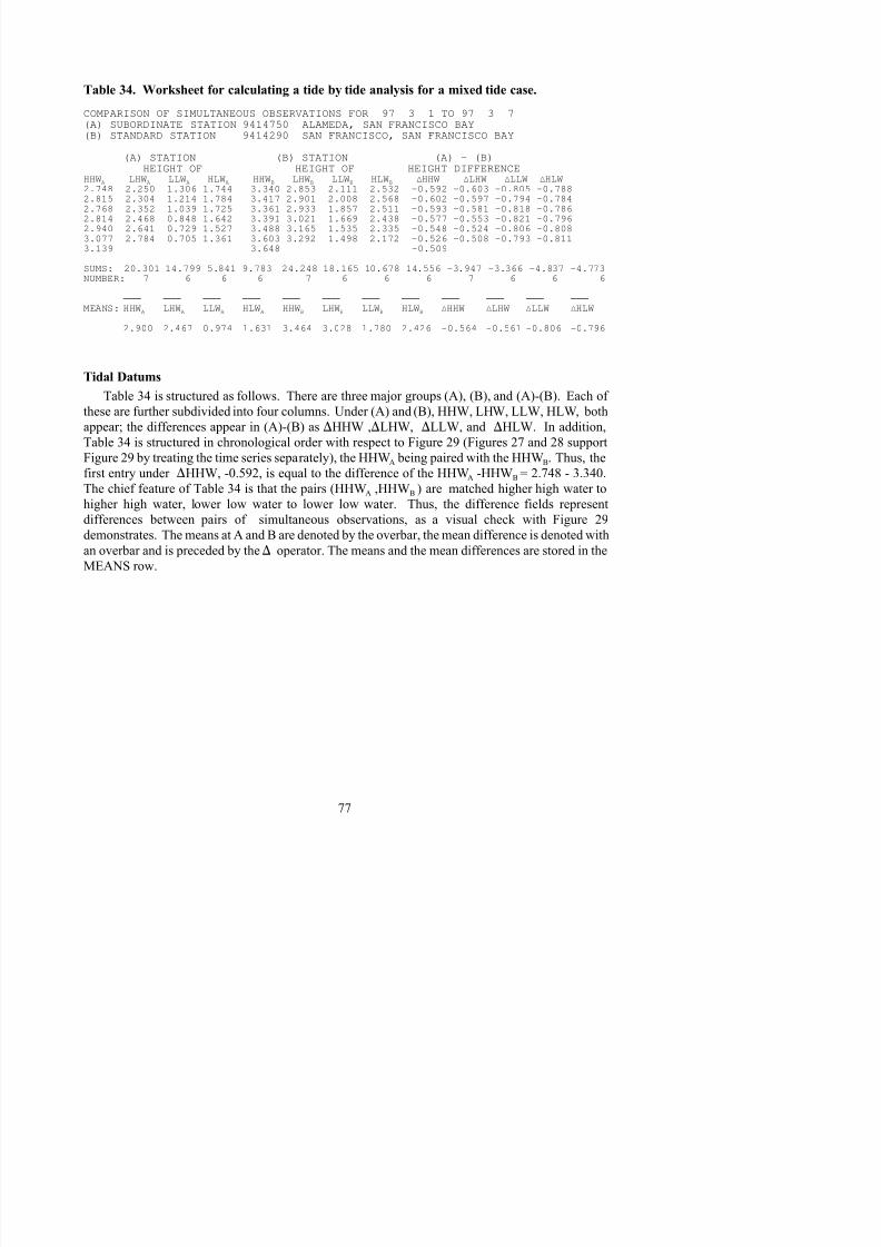
8/6/2019 Computational Techniques for Tidal Datums Handbook
http://slidepdf.com/reader/full/computational-techniques-for-tidal-datums-handbook 91/113
(A) STATION (B) STATION (A) - (B)HEIGHT OF HEIGHT OF HEIGHT DIFFERENCE
HHWA LHWA LLWA HLWA HHWB LHWB LLWB HLWB )HHW )LHW )LLW )HLW2.748 2.250 1.306 1.744 3.340 2.853 2.111 2.532 -0.592 -0.603 -0.805 -0.7882.815 2.304 1.214 1.784 3.417 2.901 2.008 2.568 -0.602 -0.597 -0.794 -0.7842.768 2.352 1.039 1.725 3.361 2.933 1.857 2.511 -0.593 -0.581 -0.818 -0.7862.814 2.468 0.848 1.642 3.391 3.021 1.669 2.438 -0.577 -0.553 -0.821 -0.7962.940 2.641 0.729 1.527 3.488 3.165 1.535 2.335 -0.548 -0.524 -0.806 -0.8083.077 2.784 0.705 1.361 3.603 3.292 1.498 2.172 -0.526 -0.508 -0.793 -0.8113.139 3.648 -0.509
SUMS: 20.301 14.799 5.841 9.783 24.248 18.165 10.678 14.556 -3.947 -3.366 -4.837 -4.773NUMBER: 7 6 6 6 7 6 6 6 7 6 6 6
SSSS SSSS SSSS SSSS SSSS SSSS SSSS SSSS SSSS SSSS SSSS SSSS
MEANS: HHWA LHWA LLWA HLWA HHWB LHWB LLWB HLWB )HHW )LHW )LLW )HLW
2.900 2.467 0.974 1.631 3.464 3.028 1.780 2.426 -0.564 -0.561 -0.806 -0.796
Tidal DatumsTable 34 is structured as follows. There are three major groups (A), (B), and (A)-(B). Each of
these are further subdivided into four columns. Under (A) and (B), HHW, LHW, LLW, HLW, both
appear; the differences appear in (A)-(B) as )HHW ,)LHW, )LLW, and )HLW. In addition,
Table 34 is structured in chronological order with respect to Figure 29 (Figures 27 and 28 support
Figure 29 by treating the time series separately), the HHWA being paired with the HHWB. Thus, the
first entry under )HHW, -0.592, is equal to the difference of the HHWA -HHWB = 2.748 - 3.340.
The chief feature of Table 34 is that the pairs (HHWA ,HHWB ) are matched higher high water to
higher high water, lower low water to lower low water. Thus, the difference fields representdifferences between pairs of simultaneous observations, as a visual check with Figure 29
demonstrates. The means at A and B are denoted by the overbar, the mean difference is denoted with
an overbar and is preceded by the ) operator. The means and the mean differences are stored in the
MEANS row.

8/6/2019 Computational Techniques for Tidal Datums Handbook
http://slidepdf.com/reader/full/computational-techniques-for-tidal-datums-handbook 92/113
Figure 27. The water level time series for Alameda with the highs and lows plotted. The data
are referenced to station datum.
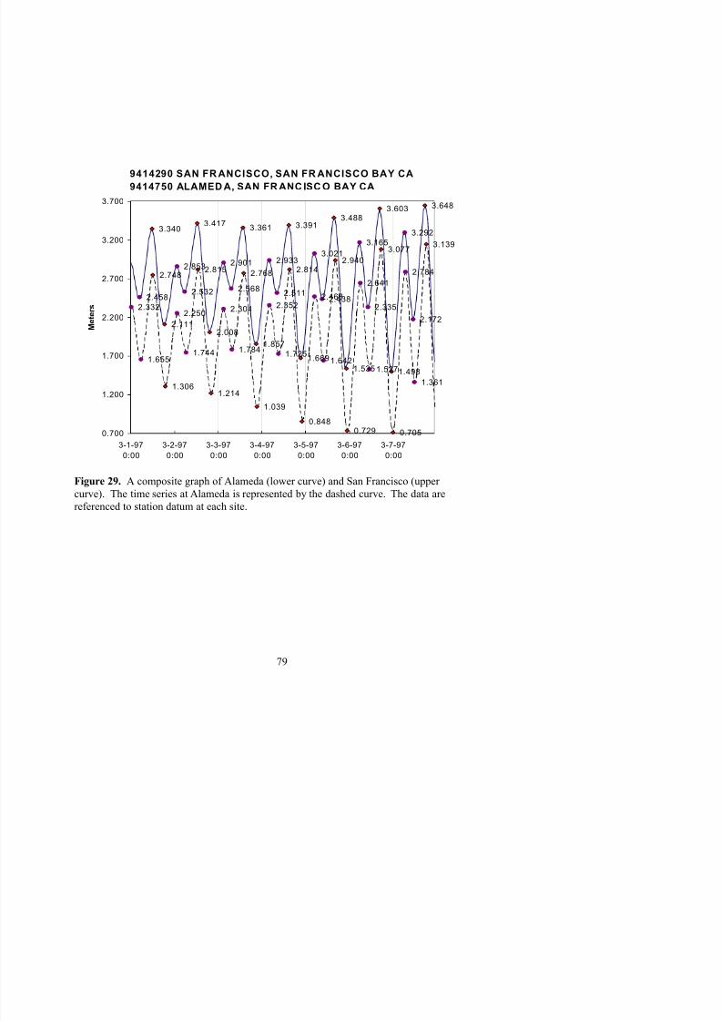
8/6/2019 Computational Techniques for Tidal Datums Handbook
http://slidepdf.com/reader/full/computational-techniques-for-tidal-datums-handbook 93/113
9414290 SAN FR ANCISCO, SAN FR ANCISCO BAY CA
9414750 ALAMED A, SAN FR ANC ISC O BAY CA
2.853 2.901 2.9333.021
3.165
3.2923.340
3.4173.361 3.391
3.488
3.603 3.648
2.4582.532 2.568
2.5112.438
2.335
2.1722.111
2.008
1.857
1.669
1.535 1.498
2.332
2.2502.304 2.352
2.468
2.641
2.7842.7482.815 2.768 2.814
2.940
3.0773.139
1.6551.744 1.784
1.7251.642
1.527
1.3611.306
1.214
1.0390.848
0.729 0.7050.700
1.200
1.700
2.200
2.700
3.200
3.700
3-1-97
0:00
3-2-97
0:00
3-3-97
0:00
3-4-97
0:00
3-5-97
0:00
3-6-97
0:00
3-7-97
0:00
M e t e r s
Figure 29. A composite graph of Alameda (lower curve) and San Francisco (upper
curve). The time series at Alameda is represented by the dashed curve. The data are
referenced to station datum at each site.
( )( )
( ) ( )
DHQ HHW LHW A A A
= × − = × − =05 05 2 900 2 467 0 216. . . . . (65)
( )
Directly from Table 34, the Diurnal High Water Inequality at A (DHQA), and the Diurnal Low
Water Inequality at A (DLQA) is given by Equations 65 and 66,
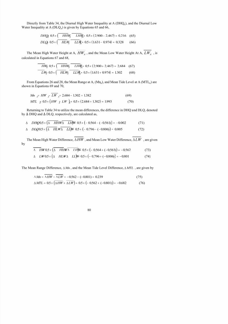
8/6/2019 Computational Techniques for Tidal Datums Handbook
http://slidepdf.com/reader/full/computational-techniques-for-tidal-datums-handbook 94/113
( ) ( )
( ) ( )
∆ ∆ ∆
∆ ∆ ∆
DHQ HHW LHW
DLQ HLW LLW
= × − = × − − − = −
= × − = × − − − =
05 05 0564 0561 0 002
05 05 0 796 0806 0 005
. . . ( . ) .
. . . ( . ) .
(71)
(72)
( )( ) ( ) DLQ HLW LLW A A A= × − = × − =05 05 1631 0 974 0328. . . . . (66)
( ) ( )
( ) ( )
HW HHW LHW
LW HLW LLW
A A A
A A A
= × + = × + =
= × + = × + =
05 05 2 900 2 467 2 684
05 05 1631 0 974 1302
. . . . .
. . . . .
(67)
(68)
( ) ( )
Mn HW LW
MTL HW LW
A A A
A A A
= − = − =
= × + = × + =
2 684 1302 1382
05 05 2 684 1302 1993
. . .
. . . . .
(69)
(70)
∆ ∆ ∆ 0 62 0801 0 239( ) ( )
( ) ( )
( ) ( )
∆ ∆ ∆
∆ ∆ ∆
HW HHW LHW
LW HLW LLW
= × + = × − + − = −
= × + = × − + − = −
05 05 0564 0561 0562
05 05 0796 0806 0801
. . . ( . ) .
. . . ( . ) .
(73)
(74)
The Mean High Water Height at A, , and the Mean Low Water Height At A, , is HW A LW Acalculated in Equations 67 and 68,
From Equations 26 and 28, the Mean Range at A, (MnA), and Mean Tide Level at A (MTLA) are
shown in Equations 69 and 70,
Returning to Table 34 to utilize the mean differences, the difference in DHQ and DLQ, denoted
by ) DHQ and ) DLQ, respectively, are calculated as,
The Mean High Water Difference, , and Mean Low Water Difference, , are given∆ HW ∆ LW by
The Mean Range Difference, , and the Mean Tide Level Difference, , are given by∆ Mn ∆ MTL
MnMn
Mn Mn
DHQ
RATIO
A
A
A
=−
=−
=∆
1382
1382 0 2391209
0216
.
. ..
.
(77)
Three quantities designated as MnRATIO, DHQRATIO, and DLQRATIO, may now be calculated as
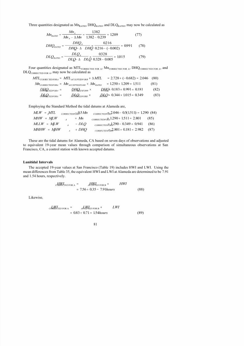
8/6/2019 Computational Techniques for Tidal Datums Handbook
http://slidepdf.com/reader/full/computational-techniques-for-tidal-datums-handbook 95/113
DHQQ
DHQ DHQ
DLQ DLQ
DLQ DLQ
RATIO
A
A
RATIO
A
A
=−
=− −
=
=−
=−
=
∆
∆
0 6
0 216 0 0020991
0328
0 328 0 0051015
.
. ( . ).
.
. ..
(78)
(79)
MTL MTL MTL
Mn Mn Mn
DHQ DHQ DHQ
DLQ DLQ DLQ
CORRECTEDFORA ACCEPTEDFORB
CORRECTEDFORA ACCEPTEDFORB RATIO
CORRECTEDFORA ACCEPTEDFORB RATIO
CORRECTEDFORA ACCEPTEDFORB RATIO
= + = + − =
= × = × =
= × = × =
= × = × =
∆ (80)
(81)
(82)
(83)
2 728 0682 2 046
1250 1209 1511
0183 0 991 0181
0 344 1015 0349
. ( . ) .
. . .
. . .
. . .
MLW MTL Mn
MHW MLW Mn
MLLW MLW DLQ
MHHW MHW DHQ
A CORRECTEDFORA CORRECTEDFORA
A A CORRECTEDFORA
A A CORRECTEDFORA
A A CORRECTEDFORA
= − = − =
= + = + =
= − = − =
= + = + =
05 2 046 05 1511 1290
1290 1511 2 801
1290 0 349 0 941
2 801 0181 2 982
. . . ( . ) .
. . .
. . .
. . .
(84)
(85)
(86)
(87)
HWI HWI HWI CORRECTED ACCEPTEDFOR A FOR B= +
Four quantities designated as MTLCORRECTED FOR A, MnCORRECTED FOR A, DHQCORRECTED FOR A, and
DLQCORRECTED FOR A, may now be calculated as
Employing the Standard Method the tidal datums at Alameda are,
These are the tidal datums for Alameda, CA based on seven days of observations and adjustedto equivalent 19-year mean values through comparison of simultaneous observations at San
Francisco, CA, a control station with known accepted datums.
Lunitidal Intervals
The accepted 19-year values at San Francisco (Table 19) includes HWI and LWI. Using the
mean differences from Table 35, the equivalent HWI and LWI at Alameda are determined to be 7.91and 1.54 hours, respectively.
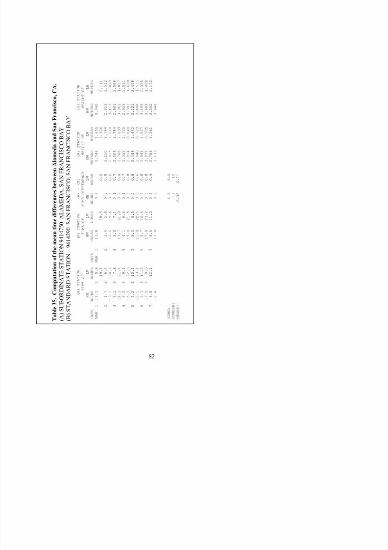
8/6/2019 Computational Techniques for Tidal Datums Handbook
http://slidepdf.com/reader/full/computational-techniques-for-tidal-datums-handbook 96/113
C o m p u t a
t i o n o f t h e m e a n t i m e d i f f e r e n c e s b e t w e e n
A l a m e d a a n d S a n F r
a n c i s c o ,
C A .
O R D I N A T E S T A T I O N 9 4 1 4 7 5 0
A L A M E D A , S A N F R
A N C I S C O B A Y
N D A R D S T
A T I O N
9 4 1 4 2 9 0 S A N F R A N C I S C O , S A N F R A N C I S C O B A Y
( A ) S T A T I O
N
( B ) S T A T
I O N
( A ) -
( B )
( A ) S T A T I O N
( B ) S T A T I O N
T I M E O F
T I M E O
F
T I M E D I F F E R E N C E
H E I G H T O F
H E I G H T O F
H W
L
W
H W
L W
H W
L W
H W
L W
H W
L W
O U R S
H O U
R S
D A T E
H O U R S
H
O U R S
H O U R S
H O U R S
M E T E R S
M E T E R S
M
E T E R S
M E T E R S
1 2 . 1
1
5
. 6
M A R
1
1 1 . 8
0 . 3
2 . 7 4 8
1 . 6 5 5
3 . 3 4 0
1 9
. 1
1 8 . 5
0 . 6
1 . 3 0 6
2 . 1 1 1
1 . 7
2
6
. 4
2
1 . 4
5 . 6
0 . 3
0 . 8
2 . 2 5 0
1 . 7 4 4
2 . 8 5 3
2 . 5 3 2
1 3 . 1
2 0
. 2
1 2 . 6
1 9 . 6
0 . 5
0 . 6
2 . 8 1 5
1 . 2 1 4
3 . 4 1 7
2 . 0 0 8
3 . 1
3
7
. 8
3
3 . 0
7 . 1
0 . 1
0 . 7
2 . 3 0 4
1 . 7 8 4
2 . 9 0 1
2 . 5 6 8
1 4 . 1
2 1
. 4
1 3 . 7
2 1 . 0
0 . 4
0 . 4
2 . 7 6 8
1 . 0 3 9
3 . 3 6 1
1 . 8 5 7
4 . 2
4
9
. 1
4
4 . 1
8 . 4
0 . 1
0 . 7
2 . 3 5 2
1 . 7 2 5
2 . 9 3 3
2 . 5 1 1
1 5 . 3
2 2
. 3
1 5 . 0
2 1 . 5
0 . 3
0 . 8
2 . 8 1 4
0 . 8 4 8
3 . 3 9 1
1 . 6 6 9
5 . 2
5
1 0
. 1
5
5 . 0
9 . 3
0 . 2
0 . 8
2 . 4 6 8
1 . 6 4 2
3 . 0 2 1
2 . 4 3 8
1 6 . 5
2 3
. 1
1 5 . 9
2 2 . 5
0 . 6
0 . 6
2 . 9 4 0
0 . 7 2 9
3 . 4 8 8
1 . 5 3 5
6 . 1
6
1 1
. 2
6
5 . 7
1 0 . 4
0 . 4
0 . 8
2 . 6 4 1
1 . 5 2 7
3 . 1 6 5
2 . 3 3 5
1 7 . 5
7
0
. 0
1 7 . 0
2 3 . 2
0 . 5
0 . 8
3 . 0 7 7
0 . 7 0 5
3 . 6 0 3
1 . 4 9 8
6 . 8
1 2
. 1
7
6 . 5
1 1 . 2
0 . 3
0 . 9
2 . 7 8 4
1 . 3 6 1
3 . 2 9 2
2 . 1 7 2
1 8 . 4
1 7 . 8
0 . 6
3 . 1 3 9
3 . 6 4 8
4 . 6
8 . 5
1 3
1 2
0 . 3 5
0 . 7 1
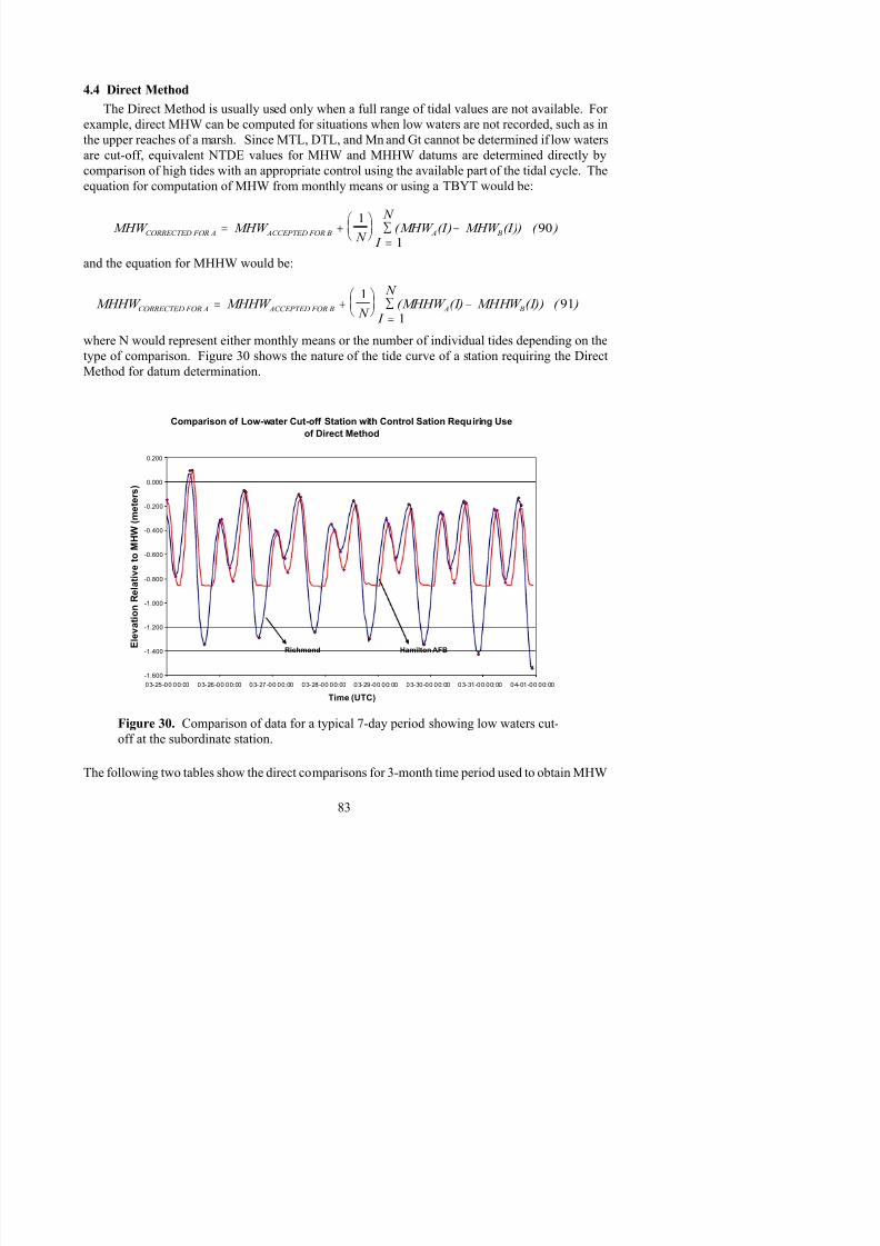
8/6/2019 Computational Techniques for Tidal Datums Handbook
http://slidepdf.com/reader/full/computational-techniques-for-tidal-datums-handbook 97/113
and MHHW datums for the station pair shown in Figure 30.
Table 36. Worksheet for computing MHW at subordinate station using the Direct Method.
(A) SUBORDINATE STATION 9415126 HAMILTON AFB, SAN FRANCISCO BAY(B) STANDARD STATION 9414863 RICHMOND, SAN FRANCISCO BAY

8/6/2019 Computational Techniques for Tidal Datums Handbook
http://slidepdf.com/reader/full/computational-techniques-for-tidal-datums-handbook 98/113
( ) ,
Mon Year M H WA B A - B
METER METER METERMar 2000 0.893 5.121 -4.228Apr 2000 0.873 5.113 -4.240May 2000 0.889 5.127 -4.238
SUMS -12.706TOTAL MONTHS 3.000MEANS -4.235ACCEPTED FOR B 5.128CORRECTED FOR A 0.893
Table 37. Worksheet for computing MHHW at subordinate station using the Direct
Method
(A) SUBORDINATE STATION 9415126 HAMILTON AFB, SAN FRANCISCO BAY(B) STANDARD STATION 9414863 RICHMOND, SAN FRANCISCO BAY
Mon Year M H H WA B A - B
METER METER METERMar 2000 1.013 5.242 -4.229Apr 2000 0.964 5.208 -4.244
May 2000 1.040 5.291 -4.251
SUMS -12.724TOTAL MONTHS 3.000MEANS -4.241ACCEPTED FOR B 5.310CORRECTED FOR A 1.069
5.0 SUMMARY
The techniques used in this handbook are the NOS methodology for the computation of tidal
datums. These techniques must be used to perform work according to NOS standards and
specifications. To perform tidal datum computations, the tides at the subordinate and control must
have similar tidal characteristics and similar ranges. The selection of the proper control station is
diffi l f di l id h f idi l i d b di l id f l h
8/6/2019 Computational Techniques for Tidal Datums Handbook
http://slidepdf.com/reader/full/computational-techniques-for-tidal-datums-handbook 99/113
more difficult for diurnal tides than for semidiurnal or mixed, because diurnal tides frequently change
their character both temporally at a site, and spatially over short distances. Lastly, all measurements
contain some error or uncertainty in their values. Vertical errors translate into horizontal errors when
surveyed to land. Horizontal errors are exacerbated by low slopes. In general, the accuracy of tidal
datums increases as the amount of data used in the computations increases.
5.1 SUMMARY OF TIDAL DATUMSRegardless of type of tide or datum computation methodology, the following tidal datums and
tidal parameters are typically desired:
Datums:
Mean Higher High Water (MHHW)
Mean High Water (MHW)
Mean Tide Level (MTL)
Diurnal Tide Level (DTL)
Mean Sea Level (MSL)
Mean Low Water (MLW)
Mean Lower Low Water (MLLW)
Ranges of Tide and Inequalities
Mean Range of Tide (Mn)
Great Diurnal Range of Tide (Gt)
Diurnal High Water Inequality (DHQ)
Diurnal Low Water Inequality (DLQ)
Lunitidal Intervals (not computed for Diurnal Tides)
High Water Interval (HWI)Low Water Interval (LWI)
Basic Procedures:
1. Make Observations - Tidal datums are computed from continuous observations of the water
level over specified lengths of time. Observations are made at specific locations called tide stations.
Each tide station consists of a water level gauge or sensor(s), a data collection platform or data logger
and data transmission system, and a set of tidal bench marks established in the vicinity of the tide
t ti NOS ll t t l l d t t 6 i t i t l
8/6/2019 Computational Techniques for Tidal Datums Handbook
http://slidepdf.com/reader/full/computational-techniques-for-tidal-datums-handbook 100/113
station. NOS collects water level data at 6-minute intervals.
2. Tabulate the Tide - Once water level observations are quality controlled and any small gaps
filled, the data are processed by tabulating the high and low tides and hourly heights for each day.
Tidal parameters from these daily tabulations of the tide are then reduced to mean values, typically
on a calendar month basis for longer period records or over a few days or weeks for shorter-term
records.
3. Compute Tidal Datums - First reduction tidal datums are determined directly by meaning
values of the tidal parameters over a 19-year NDTE. Equivalent NDTE tidal datums are computed
from tide stations operating for shorter time periods through comparison of simultaneous data
between the short-term station and a long term station.
4. Compute Bench Mark Elevations - Once the tidal datums are computed from the tabulations,
the elevations are transferred to the bench marks established on the land through the elevationdifferences established by differential leveling between the tide gauge sensor “zero” and the bench
marks during the station operation. The bench mark elevations and descriptions are disseminated by
NOS through a published bench mark sheet for each station. Connections between tidal datum
elevations and geodetic elevations are obtained after leveling between tidal bench marks and geodetic
network bench marks. Traditionally, this has been accomplished using differential leveling, however
GPS surveying techniques can also be used (NGS, 1997).
The locations of tide stations are organized into a hierarchy:
Control tide stations are generally those which have been operated for 19 or more years, are
expected to continuously operate in the future, and are used to obtain a continuous record of the water
levels in a locality. Control tide stations are sited to provide datum control for national applications,
and located in as many places as needed for datum control.
Secondary water level stations are those which are operated for less than 19 years but more than
1 year, and have a planned finite lifetime. Secondary stations provide control in bays and estuarieswhere localized tidal effects are not realized at the nearest control station. Observations at a
secondary station are not usually sufficient for a precise independent determination of tidal datums,
but when reduced by comparison with simultaneous observations at a suitable control tide station
locations for network coverage. The site selection criteria include spatial coverage of significant
changes in tidal characteristics such as: changes in tide type, changes in range of tide, changes in time
of tide, changes in daily mean sea level and changes in long term mean sea level trends. Other
criteria include coverage of critical navigation areas and transitional zones, historical sites, proximity
to the geodetic network, and the availability of existing structures, such as piers suitable for thelocation of the scientific equipment
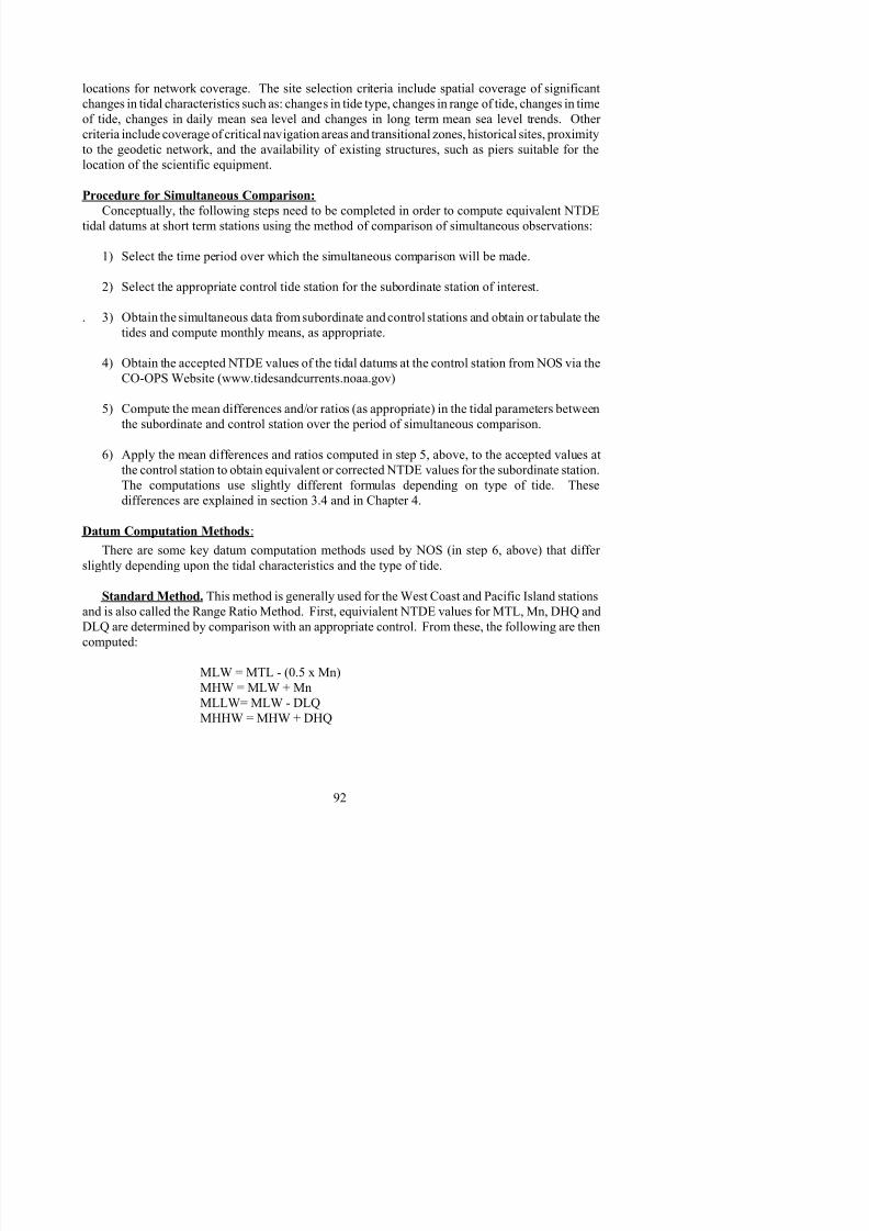
8/6/2019 Computational Techniques for Tidal Datums Handbook
http://slidepdf.com/reader/full/computational-techniques-for-tidal-datums-handbook 101/113
location of the scientific equipment.
Procedure for Simultaneous Comparison:
Conceptually, the following steps need to be completed in order to compute equivalent NTDE
tidal datums at short term stations using the method of comparison of simultaneous observations:
1) Select the time period over which the simultaneous comparison will be made.
2) Select the appropriate control tide station for the subordinate station of interest.
. 3) Obtain the simultaneous data from subordinate and control stations and obtain or tabulate the
tides and compute monthly means, as appropriate.
4) Obtain the accepted NTDE values of the tidal datums at the control station from NOS via the
CO-OPS Website (www.tidesandcurrents.noaa.gov)
5) Compute the mean differences and/or ratios (as appropriate) in the tidal parameters between
the subordinate and control station over the period of simultaneous comparison.
6) Apply the mean differences and ratios computed in step 5, above, to the accepted values at
the control station to obtain equivalent or corrected NTDE values for the subordinate station.
The computations use slightly different formulas depending on type of tide. These
differences are explained in section 3.4 and in Chapter 4.
Datum Computation Methods:
There are some key datum computation methods used by NOS (in step 6, above) that differ
slightly depending upon the tidal characteristics and the type of tide.
Standard Method. This method is generally used for the West Coast and Pacific Island stations
and is also called the Range Ratio Method. First, equivialent NTDE values for MTL, Mn, DHQ andDLQ are determined by comparison with an appropriate control. From these, the following are then
computed:
Modified-Range Ratio Method. This method is generally used for the East Coast, Gulf Coast
and Caribbean Island stations. First, equivalent NTDE values for MTL, DTL, Mn and Gt as
determined by comparison with an appropriate control. The difference from the Standard Method
is that ratios of the DHQ and DLQ values are not used to compute MHHW and MLLW because
numerically the values are very small for semidiurnal tide areas. A Gt ratio about DTL is usedinstead. From these, the following are computed:
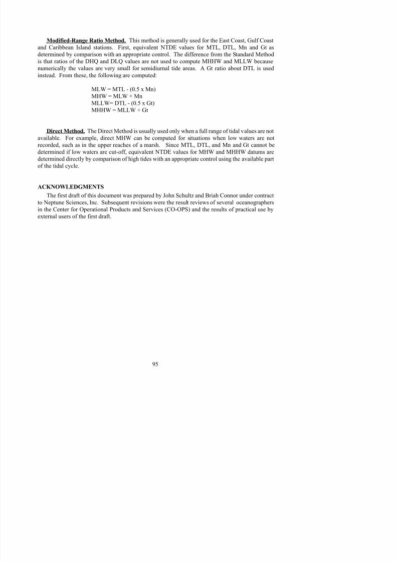
8/6/2019 Computational Techniques for Tidal Datums Handbook
http://slidepdf.com/reader/full/computational-techniques-for-tidal-datums-handbook 102/113
instead. From these, the following are computed:
MLW = MTL - (0.5 x Mn)
MHW = MLW + Mn
MLLW= DTL - (0.5 x Gt)
MHHW = MLLW + Gt
Direct Method. The Direct Method is usually used only when a full range of tidal values are not
available. For example, direct MHW can be computed for situations when low waters are not
recorded, such as in the upper reaches of a marsh. Since MTL, DTL, and Mn and Gt cannot be
determined if low waters are cut-off, equivalent NTDE values for MHW and MHHW datums are
determined directly by comparison of high tides with an appropriate control using the available part
of the tidal cycle.
ACKNOWLEDGMENTS
The first draft of this document was prepared by John Schultz and Briah Connor under contract
to Neptune Sciences, Inc. Subsequent revisions were the result reviews of several oceanographers
in the Center for Operational Products and Services (CO-OPS) and the results of practical use by
external users of the first draft.

8/6/2019 Computational Techniques for Tidal Datums Handbook
http://slidepdf.com/reader/full/computational-techniques-for-tidal-datums-handbook 103/113
8/6/2019 Computational Techniques for Tidal Datums Handbook
http://slidepdf.com/reader/full/computational-techniques-for-tidal-datums-handbook 104/113
Schureman, P., Manual of Harmonic Analysis and Prediction of Tides, Special Publication No. 98
(1940), U.S. Coast and Geodetic Survey, U.S. Govt. Printing Office, revised ed.,1941.
Swanson, R.L., Variability of Tidal Datums and Accuracy in Determining Datums from Short Series
of Observations, NOAA Tech. Rep. NOS 64, Silver Spring, MD, pp. 41, 1974.

8/6/2019 Computational Techniques for Tidal Datums Handbook
http://slidepdf.com/reader/full/computational-techniques-for-tidal-datums-handbook 105/113
Zervas, C., Sea Level Variations of the United States 1854 - 1999, NOAA Technical Report NOS
CO-OPS 36, Silver Spring, MD, pp186, 2001.

8/6/2019 Computational Techniques for Tidal Datums Handbook
http://slidepdf.com/reader/full/computational-techniques-for-tidal-datums-handbook 106/113
Appendix 1:
EXAMPLES OF TIDAL DATUM COMPUTATION
SPREADSHEETS
A. SEMIDIURNAL TIDE TYPE: MODIFIED RANGE RATIO
METHOD
B. MIXED TIDE TYPE: STANDARD METHOD
SUBORDINATE STATION A: FORT PULASKI, GA ELEVATIONS IN METERS, TIME IN HOURS
CONTROL STATION B: CHARLESTON, SC
MTL DTL HWIStation A Station B A - B Station A Station B A - B Station A Station B A - B
1997 03 2.156 1.662 0.494 2.159 1.672 0.487 0.54 0.41 0.131997 04 2.248 1.751 0.497 2.259 1.763 0.496 0.55 0.41 0.14
1997 05 2 188 1 673 0 515 2 208 1 699 0 509 0 54 0 41 0 13
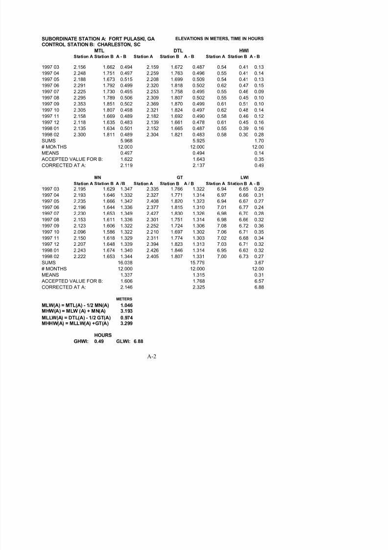
8/6/2019 Computational Techniques for Tidal Datums Handbook
http://slidepdf.com/reader/full/computational-techniques-for-tidal-datums-handbook 107/113
1997 05 2.188 1.673 0.515 2.208 1.699 0.509 0.54 0.41 0.13
1997 06 2.291 1.792 0.499 2.320 1.818 0.502 0.62 0.47 0.15
1997 07 2.225 1.730 0.495 2.253 1.758 0.495 0.55 0.46 0.09
1997 08 2.295 1.789 0.506 2.309 1.807 0.502 0.55 0.45 0.10
1997 09 2.353 1.851 0.502 2.369 1.870 0.499 0.61 0.51 0.10
1997 10 2.305 1.807 0.498 2.321 1.824 0.497 0.62 0.48 0.14
1997 11 2.158 1.669 0.489 2.182 1.692 0.490 0.58 0.46 0.121997 12 2.118 1.635 0.483 2.139 1.661 0.478 0.61 0.45 0.16
1998 01 2.135 1.634 0.501 2.152 1.665 0.487 0.55 0.39 0.16
1998 02 2.300 1.811 0.489 2.304 1.821 0.483 0.58 0.30 0.28
SUMS 5.968 5.925 1.70
# MONTHS 12.000 12.000 12.00
MEANS 0.497 0.494 0.14
ACCEPTED VALUE FOR B: 1.622 1.643 0.35
CORRECTED AT A: 2.119 2.137 0.49
MN GT LWI
Station A Station B A /B Station A Station B A / B Station A Station B A - B
1997 03 2.195 1.629 1.347 2.335 1.766 1.322 6.94 6.65 0.29
1997 04 2.193 1.646 1.332 2.327 1.771 1.314 6.97 6.66 0.31
1997 05 2.235 1.666 1.342 2.408 1.820 1.323 6.94 6.67 0.27
1997 06 2.196 1.644 1.336 2.377 1.815 1.310 7.01 6.77 0.24
1997 07 2.230 1.653 1.349 2.427 1.830 1.326 6.98 6.70 0.28
1997 08 2.153 1.611 1.336 2.301 1.751 1.314 6.98 6.66 0.32
1997 09 2.123 1.606 1.322 2.252 1.724 1.306 7.08 6.72 0.36
1997 10 2.096 1.586 1.322 2.210 1.697 1.302 7.06 6.71 0.35
1997 11 2.150 1.618 1.329 2.311 1.774 1.303 7.02 6.68 0.34
1997 12 2.207 1.648 1.339 2.394 1.823 1.313 7.03 6.71 0.32
1998 01 2.243 1.674 1.340 2.426 1.846 1.314 6.95 6.63 0.32
1998 02 2.222 1.653 1.344 2.405 1.807 1.331 7.00 6.73 0.27
SUMS 16.038 15.779 3.67
# MONTHS 12.000 12.000 12.00
MEANS 1.337 1.315 0.31ACCEPTED VALUE FOR B: 1.606 1.768 6.57
CORRECTED AT A: 2.146 2.325 6.88
METERS
SUBORDINATE STATION A: ALAMEDA, CA ELEVATIONS IN METERS;TIMES IN HOURS
CONTROL STATION B: SAN FRANCISCO, CAMTL MN HWI
Station A Station B A - B Station A Station B A /B Station A Station B A - B
1997 03 2.058 2.731 -0.673 1.503 1.257 1.196 0.54 0.41 0.13
1997 04 1.978 2.648 -0.670 1.543 1.292 1.194 0.55 0.41 0.14
1997 05 2 066 2 741 0 675 1 533 1 294 1 185 0 54 0 41 0 13

8/6/2019 Computational Techniques for Tidal Datums Handbook
http://slidepdf.com/reader/full/computational-techniques-for-tidal-datums-handbook 108/113
1997 05 2.066 2.741 -0.675 1.533 1.294 1.185 0.54 0.41 0.13
1997 06 2.131 2.809 -0.678 1.537 1.306 1.177 0.62 0.47 0.15
1997 07 2.147 2.830 -0.683 1.527 1.300 1.175 0.55 0.46 0.09
1997 08 2.196 2.882 -0.686 1.514 1.301 1.164 0.55 0.45 0.10
1997 09 2.199 2.878 -0.679 1.492 1.272 1.173 0.61 0.51 0.10
1997 10 2.216 2.905 -0.689 1.503 1.279 1.175 0.62 0.48 0.14
1997 11 2.298 2.995 -0.697 1.525 1.296 1.177 0.58 0.46 0.121997 12 2.267 2.970 -0.703 1.544 1.311 1.178 0.61 0.45 0.16
1998 01 2.303 3.001 -0.698 1.533 1.287 1.191 0.55 0.39 0.16
1998 02 2.414 3.103 -0.689 1.336 1.101 1.213 0.58 0.30 0.28
SUMS -8.220 14.197 1.70
# MONTHS 12.000 12.000 12.00MEANS -0.685 1.183 0.14
ACCEPTED VALUE FOR B: 2.728 1.250 0.35
CORRECTED AT A: 2.043 1.479 0.49
DHQ DLQ LWI
Station A Station B A /B Station A Station B A /B Station A Station B A - B
1997 03 0.132 0.122 1.082 0.247 0.242 1.021 6.94 6.65 0.29
1997 04 0.116 0.117 0.991 0.293 0.292 1.003 6.97 6.66 0.31
1997 05 0.166 0.162 1.025 0.320 0.322 0.994 6.94 6.67 0.27
1997 06 0.218 0.213 1.023 0.347 0.352 0.986 7.01 6.77 0.24
1997 07 0.225 0.219 1.027 0.340 0.344 0.988 6.98 6.70 0.28
1997 08 0.184 0.176 1.045 0.275 0.274 1.004 6.98 6.66 0.321997 09 0.116 0.113 1.027 0.203 0.203 1.000 7.08 6.72 0.36
1997 10 0.105 0.101 1.040 0.217 0.219 0.991 7.06 6.71 0.35
1997 11 0.166 0.162 1.025 0.319 0.324 0.985 7.02 6.68 0.34
1997 12 0.224 0.217 1.032 0.366 0.366 1.000 7.03 6.71 0.32
1998 01 0.215 0.213 1.009 0.328 0.337 0.973 6.95 6.63 0.32
1998 02 0.187 0.183 1.022 0.234 0.261 0.897 7.00 6.73 0.27
SUMS 12.349 11.841 3.67
# MONTHS 12.000 12.000 12.00
MEANS 1.029 0.987 0.31ACCEPTED VALUE FOR B: 0.183 0.344 6.57
CORRECTED AT A: 0.188 0.339 6.88
S

8/6/2019 Computational Techniques for Tidal Datums Handbook
http://slidepdf.com/reader/full/computational-techniques-for-tidal-datums-handbook 109/113

8/6/2019 Computational Techniques for Tidal Datums Handbook
http://slidepdf.com/reader/full/computational-techniques-for-tidal-datums-handbook 110/113
Appendix 2:
EXAMPLE OF TIDAL DATUM COMPUTATION
SPREADSHEET FOR TIDE BY TIDE COMPARISON
TIDES: Comparison of Simultaneous Observations (Tide by Tide)PAGE 1
A) Subordinate Station: 9414750 Alameda, SanFrancisco Bay
B) Standard Station: 9414290 San Francisco, San Francisco Bay
Lat: 37 46.3 n
Lat: 37 48.4 n
Time Meridian:
units: meters
Long: 122 17.9 w
Long: 122 27.9 w
(A) 0° (UTC) (B) 0° (UTC)
Date (A) Station = (B) Station = (A) Station = (B) Station = (A) - (B) ( A) - (B) (A) - (B)
TIME TIME HEIGHT (STATION DATUM) HEIGHT (MLLW) TIME DIFFERENCE (minutes) HEIGHT DIFFERENCE
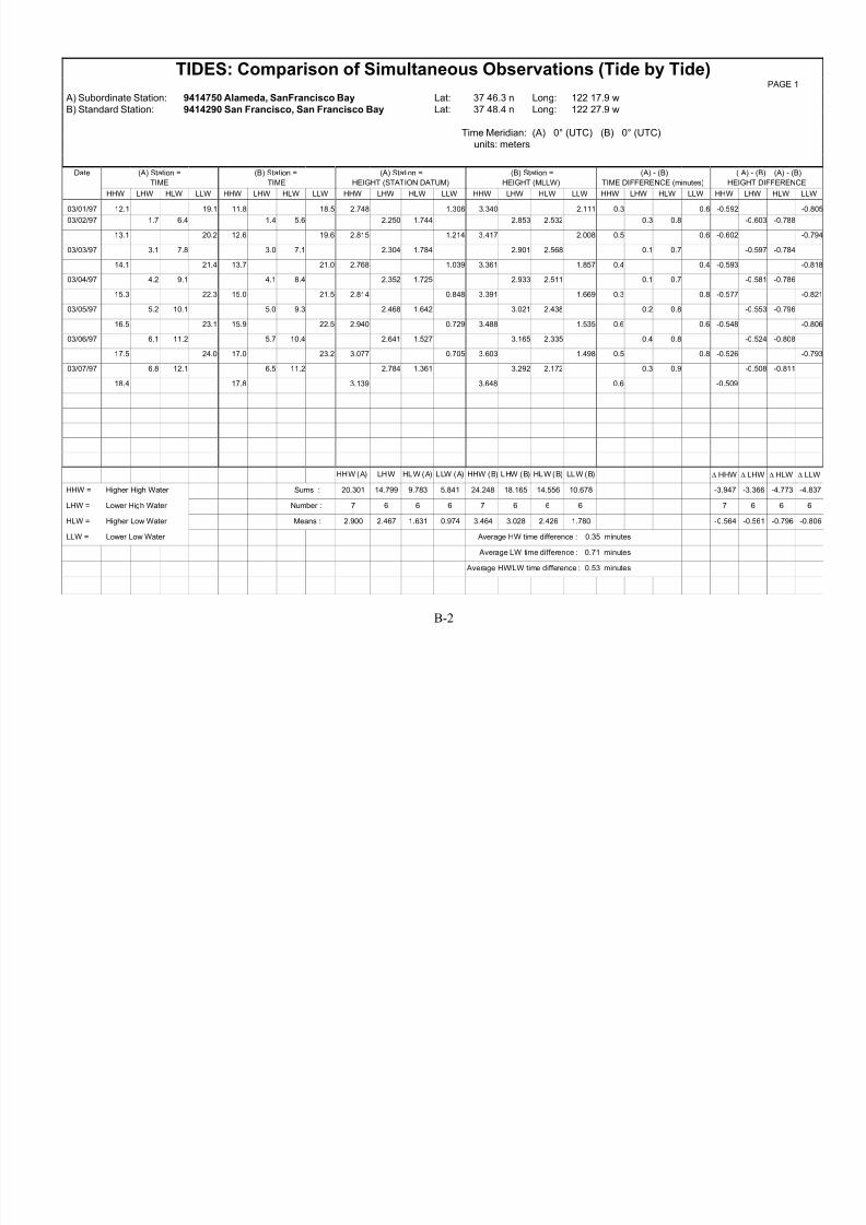
8/6/2019 Computational Techniques for Tidal Datums Handbook
http://slidepdf.com/reader/full/computational-techniques-for-tidal-datums-handbook 111/113
B-2
TIME TIME HEIGHT (STATION DATUM) HEIGHT (MLLW) TIME DIFFERENCE (minutes) HEIGHT DIFFERENCE
HHW LHW HLW LLW HHW LHW HLW LLW HHW LHW HLW LLW HHW LHW HLW LLW HHW LHW HLW LLW HHW LHW HLW LLW
03/01/97 12.1 19.1 11.8 18.5 2.748 1.306 3.340 2.111 0.3 0.6 -0.592 -0.805
03/02/97 1.7 6.4 1.4 5.6 2.250 1.744 2.853 2.532 0.3 0.8 -0.603 -0.788
13.1 20.2 12.6 19.6 2.815 1.214 3.417 2.008 0.5 0.6 -0.602 -0.794
03/03/97 3.1 7.8 3.0 7.1 2.304 1.784 2.901 2.568 0.1 0.7 -0.597 -0.784
14.1 21.4 13.7 21.0 2.768 1.039 3.361 1.857 0.4 0.4 -0.593 -0.818
03/04/97 4.2 9.1 4.1 8.4 2.352 1.725 2.933 2.511 0.1 0.7 -0.581 -0.786
15.3 22.3 15.0 21.5 2.814 0.848 3.391 1.669 0.3 0.8 -0.577 -0.821
03/05/97 5.2 10.1 5.0 9.3 2.468 1.642 3.021 2.438 0.2 0.8 -0.553 -0.796
16.5 23.1 15.9 22.5 2.940 0.729 3.488 1.535 0.6 0.6 -0.548 -0.806
03/06/97 6.1 11.2 5.7 10.4 2.641 1.527 3.165 2.335 0.4 0.8 -0.524 -0.808
17.5 24.0 17.0 23.2 3.077 0.705 3.603 1.498 0.5 0.8 -0.526 -0.793
03/07/97 6.8 12.1 6.5 11.2 2.784 1.361 3.292 2.172 0.3 0.9 -0.508 -0.811
18.4 17.8 3.139 3.648 0.6 -0.509
HHW (A) LHW HLW (A) LLW (A) HHW (B) LHW (B) HLW (B) LLW (B) ∆ HHW ∆ LHW ∆ HLW ∆ LLW
HHW = Higher High Water Sums : 20.301 14.799 9.783 5.841 24.248 18.165 14.556 10.678 -3.947 -3.366 -4.773 -4.837
LHW = Lower High Water Number : 7 6 6 6 7 6 6 6 7 6 6 6
HLW = Higher Low Water Means : 2.900 2.467 1.631 0.974 3.464 3.028 2.426 1.780 -0.564 -0.561 -0.796 -0.806
LLW = Lower Low Water Average HW time difference : 0.35 minutes
Average LW time difference : 0.71 minutes
Average HW/LW time difference : 0.53 minutes
TIDES: Comparison of Simultaneous Observations (Tide by Tide)
Eq. #
0.217 = DHQ (A) = 0.5*(HHW (A) - LHW (A)) 22 Standard Method: Datum Planes (relative to station datum)
0.329 = DLQ (A) = 0.5*(HLW (A) - LLW (A)) 23 2.984 = MHHW (A) = MHW (A) + DHQ corrected for A 87
2.683 = HW (A) = 0.5*(HHW (A) + LHW (A)) 24 2.802 = MHW (A) = MLW (A) + MN corrected for A 851.302 = LW (A) = 0.5*(HLW (A) + LLW (A)) 25 1.291 = MLW (A) = MTL corrected for A - 0.5 * MN corrected for A 84
1.927 = Gt (A) = HHW (A) - LLW (A) 26 0.941 = MLLW (A) = MLW (A) - DLQ corrected for A 86
1 381 = Mn (A) = HW (A) - LW (A) 27
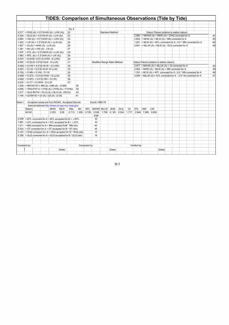
8/6/2019 Computational Techniques for Tidal Datums Handbook
http://slidepdf.com/reader/full/computational-techniques-for-tidal-datums-handbook 112/113
B-3
1.381 = Mn (A) = HW (A) - LW (A) 27
1.937 = DTL (A) = 0.5*(HHW (A) + LLW (A)) 28
1.993 = MTL (A) = 0.5*(HW (A) + LW (A)) 29
-0.001 = D DHQ =0.5*( D HHW - D LHW) 30
0.005 = D DLQ= 0.5*(D HLW - D LLW) 31 Modified Range Ratio Method: Datum Planes (relative to station datum)
-0.562 = D HW = 0.5*(D HHW + D LHW) 32 2.977 = MHHW (A) = MLLW (A) + Gt corrected for A 62
-0.801 = D LW = 0.5*(D HLW +D LLW) 33 2.802 = MHW (A) = MLW (A) + MN corrected for A 49
0.238 = D MN = D HW - D LW 34 1.291 = MLW (A) = MTL corrected for A - 0.5 * MN corrected for A 48
-0.685 = D DTL = 0.5*(D HHW + D LLW) 35 0.945 = MLLW (A) = DTL corrected for A - 0.5* Gt corrected for A 61
-0.682 = D MTL = 0.5*(D HW + D LW) 36
0.242 = D GT = D HHW - D LLW 37
1.209 = MN RATIO = MN (A) / (MN (A) - D MN) 38
0.993 = DHQ RATIO = DHQ (A) / (DHQ (A) - D DHQ) 39
1.017 = DLQ RATIO = DLQ (A) / (DLQ (A) - DDLQ) 40
1.144 = Gt RATIO = Gt (A) / (Gt (A) - D Gt) 41
Note 1: Accepted values are from NOAA, Accepted Datums Epoch:1960-78
Internet address:http://www.co-ops.nos.noaa.gov/
Station MHW MLW MSL Mn MTL MHHW MLLW DHQ DLQ Gt DTL HWI LWI
94142 3.353 2:28 2.713 1.250 2.728 3.536 1.759 0.183 0.344 1.777 2.646 7.560 0.830
Eq#
2.046 = MTL corrected for A = MTL accepted for B + ∆ MTL 42
1.961 = DTL corrected for A = DTL accepted for B + ∆ DTL 43
1.511 = MN corrected for A = MN accepted forB * MN ratio 44
2.033 = GT corrected for A = GT accepted for B * GT ratio 45
0.182 = DHQ corrected for A = DHQ accepted for B * DHQ ratio 150.350 = DLQ corrected for A = DLQ accepted for B * DLQ ratio 16
Compiled by: Computed by: Verified by:
(Date) (Date) (Date)

8/6/2019 Computational Techniques for Tidal Datums Handbook
http://slidepdf.com/reader/full/computational-techniques-for-tidal-datums-handbook 113/113