Computational Studies of Horizontal Axis Wind Turbines Ph.D. Oral Defense Presented By Guanpeng Xu Advisor: Dr. L Sankar School of Aerospace Engineering

Computational Studies of Horizontal Axis Wind Turbines

Ph.D. Oral Defense

Presented By

Guanpeng XuAdvisor: Dr. L Sankar

School of Aerospace EngineeringGeorgia Institute of Technology

This work was supported by NRELMonitor: Dr. Scott Schreck

Georgia Tech School of Aerospace Engineering

Outline of the Presentation

• Importance of wind energy

• Overview of the present research

• Methodology and numerical procedure

• Results and discussions

• Conclusions and recommendations


Importance of Wind Energy

• Wind Energy is a clean source of energy.

• Wind Energy is renewable.

• It may be used to augment to other forms of energy,

e.g. fossil fuel.

• Many parts of US and other countries have sites

with high wind, making wind energy based power

generation feasible.


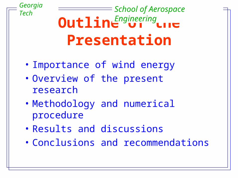
Existing Approaches for Wind Turbine Performance

• Blade Element Methods– 2-D strip theory – Analytical inflow – Fast and is in routine use – Require table look up for airfoil data– Modeling tip losses and 3-D stall effects remain unsolved

issues • Navier-Stokes Simulations

– Can capture all the physics from first principles– Can provide high-quality details of the flow field– Require large computer time

• Hybrid Methods


Hybrid Methodology

• The flow field is made of

– a viscous region near the blade(s)

– A potential flow region that propagates the blade circulation and thickness effects to the far field

– A Lagrangean representation of the tip vortex, and concentrated vorticity shed from nearby bluff bodies such as the tower

• This method is unsteady, compressible, and does not have singularities near separation lines

N-S zone

Potential Flow Zone Tip Vortex


A hybrid technique offers the following capabilities:

• It can capture viscous phenomena efficiently.• Tip vortex is modeled accurately.• There is no need for analytical inflow models.• It is applicable to steady and unsteady HAWT

applications.• High order accuracy solutions are obtained with

small CPU time.

Hybrid Solver Versus Others



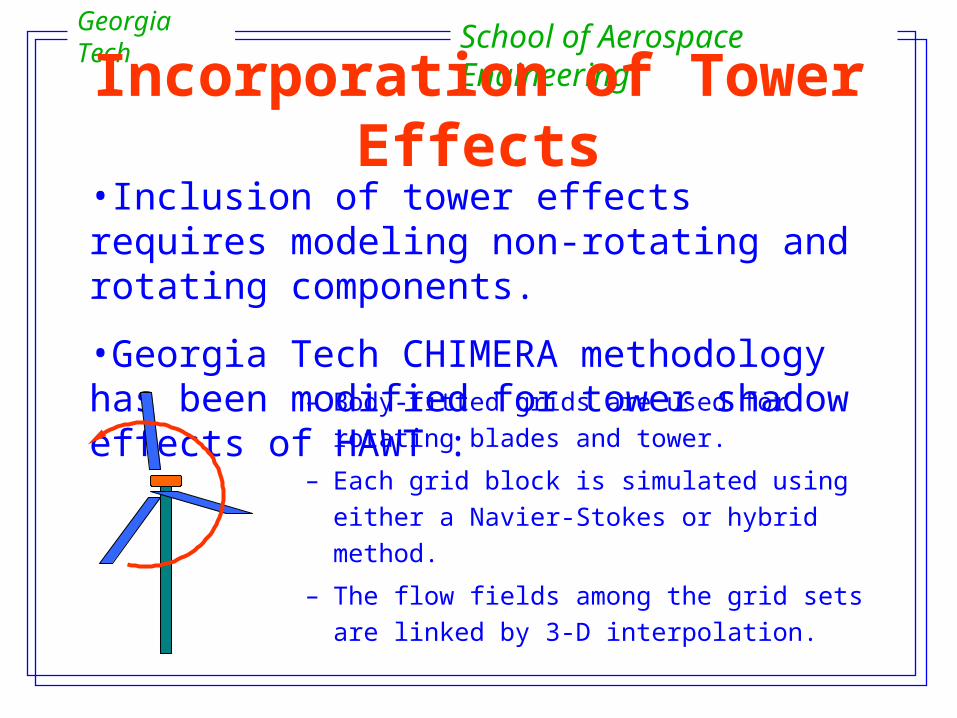
Incorporation of Tower Effects

– Body-fitted grids are used for rotating

blades and tower.

– Each grid block is simulated using either a

Navier-Stokes or hybrid method.

– The flow fields among the grid sets are

linked by 3-D interpolation.

•Inclusion of tower effects requires modeling non-rotating and rotating components.

•Georgia Tech CHIMERA methodology has been modified for tower shadow effects of HAWT :

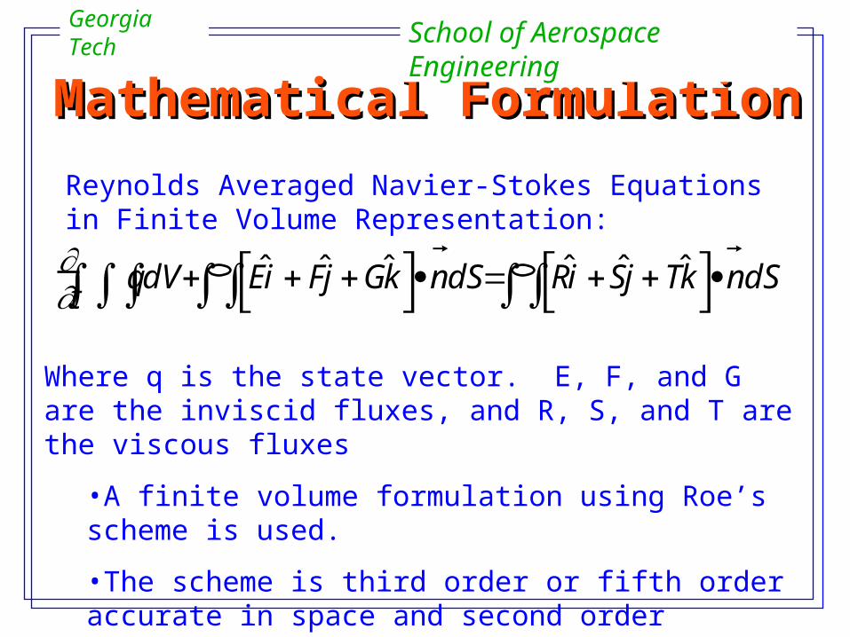
Mathematical FormulationMathematical Formulation

Reynolds Averaged Navier-Stokes Equations in Finite Volume Representation:

t

qdV Eˆ i Fˆ j Gˆ k n dS Rˆ i Sˆ j T ˆ k n dS

Where q is the state vector. E, F, and G are the inviscid fluxes, and R, S, and T are the viscous fluxes

•A finite volume formulation using Roe’s scheme is used.

•The scheme is third order or fifth order accurate in space and second order accurate in time.


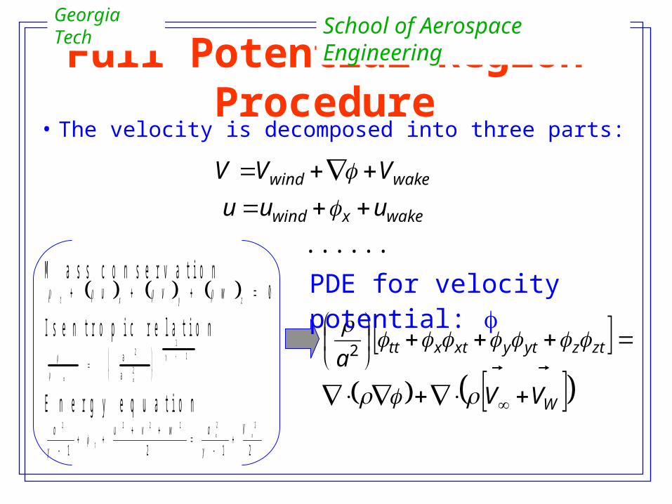
Full Potential Region Procedure• The velocity is decomposed into three parts:

W

ztzytyxtxtt

VV

a

2

M a s s c o n s e r v a t i o n 0 zyxt wvu

I s e n t r o p i c r e l a t i o n

a 2

a 2

1 1

E n e r g y e q u a t i o n

2121

222222

Vawvua

t

PDE for velocity potential:

......wakexwind

wakewind

uuu

VVV


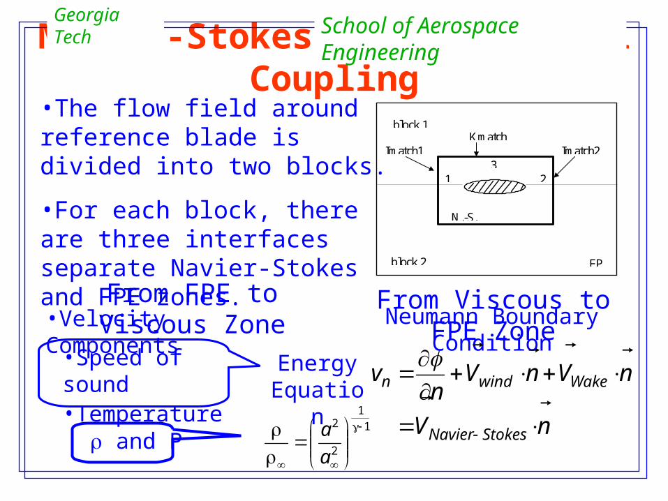
Navier-Stokes/Full Potential Coupling

N.-S.

FP

Kmatch

block 2

block 1

1 23

Imatch1 Imatch2

•The flow field around reference blade is divided into two blocks.

•For each block, there are three interfaces separate Navier-Stokes and FPE zones.

From FPE to Viscous Zone From Viscous to FPE Zone•Velocity Components

•Speed of sound•Temperature

Energy Equation

and P1

1

2

2

a

a

Neumann Boundary Condition

nV

nVnVn

v

StokesNavier

Wakewindn


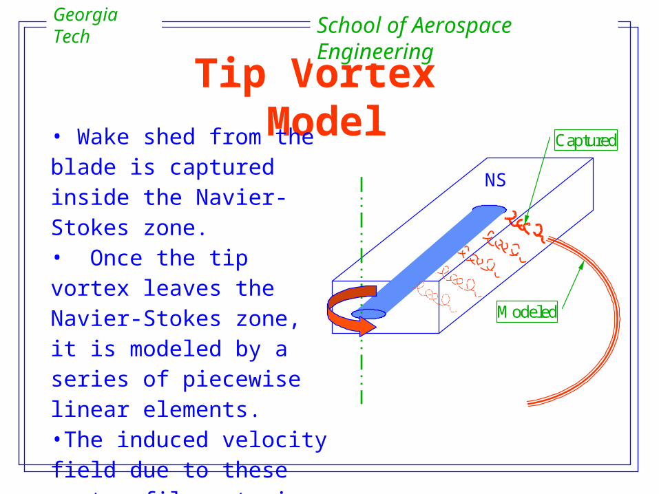
Tip Vortex Model

• Wake shed from the blade is captured inside the Navier-Stokes zone.• Once the tip vortex leaves the Navier-Stokes zone, it is modeled by a series of piecewise linear elements. •The induced velocity field due to these vortex filaments is calculated by Biot-Savart law where needed.


NS

Captured

Modeled

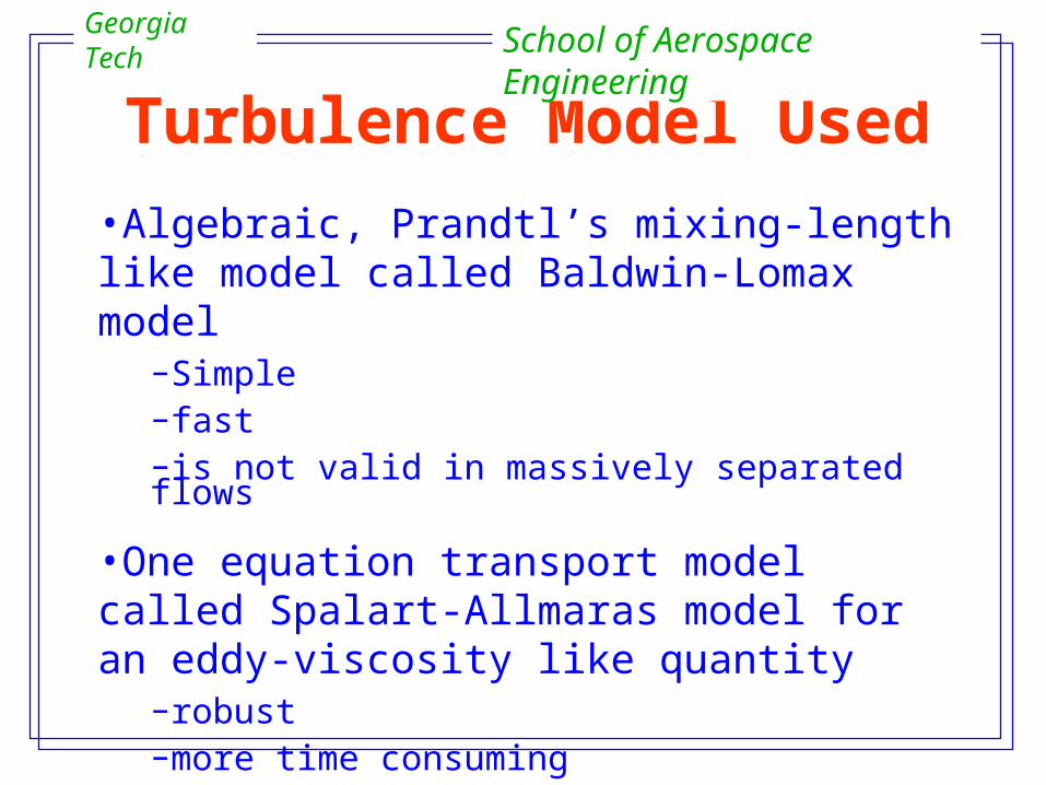
Turbulence Model Used


•Algebraic, Prandtl’s mixing-length like model called Baldwin-Lomax model

–Simple–fast–is not valid in massively separated flows

•One equation transport model called Spalart-Allmaras model for an eddy-viscosity like quantity

–robust–more time consuming–in wide use for separated and unsteady flows

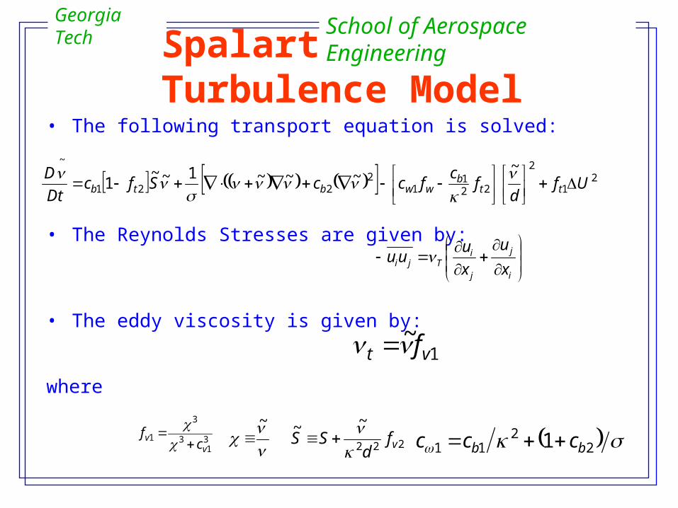
Spalart-Allmaras Turbulence Model• The following transport equation is solved:

• The Reynolds Stresses are given by:

• The eddy viscosity is given by:

where

21

2

221

12

221

~ ~~~~1~~

1 Ufd

fc

fccSfcDt

Dtt

bwwbtb

i

j

j

iTji x

u

x

uuu

1~

vt f

31

3

3

1v

vc

f

~

222

~~vf

dSS

22

11 1 bb ccc


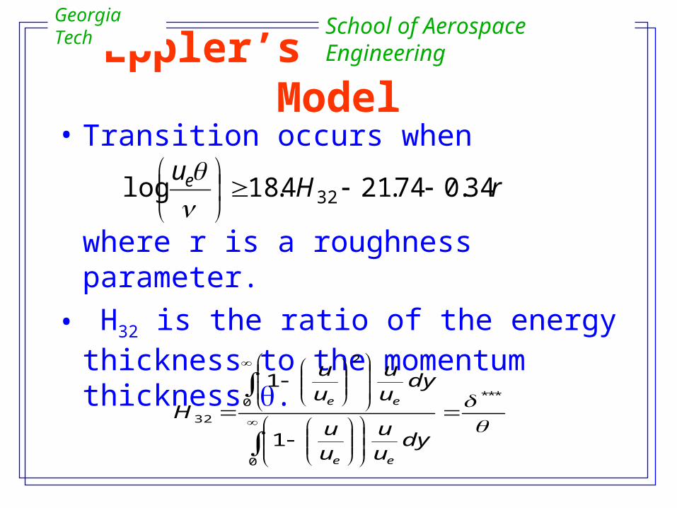
Eppler’s Transition Model

• Transition occurs when

where r is a roughness parameter.

• H32 is the ratio of the energy thickness to the momentum thickness .

rHue 34.074.214.18log 32

***

0

0

2

32

1

1

dyuu

uu

dyuu

uu

H

ee

ee


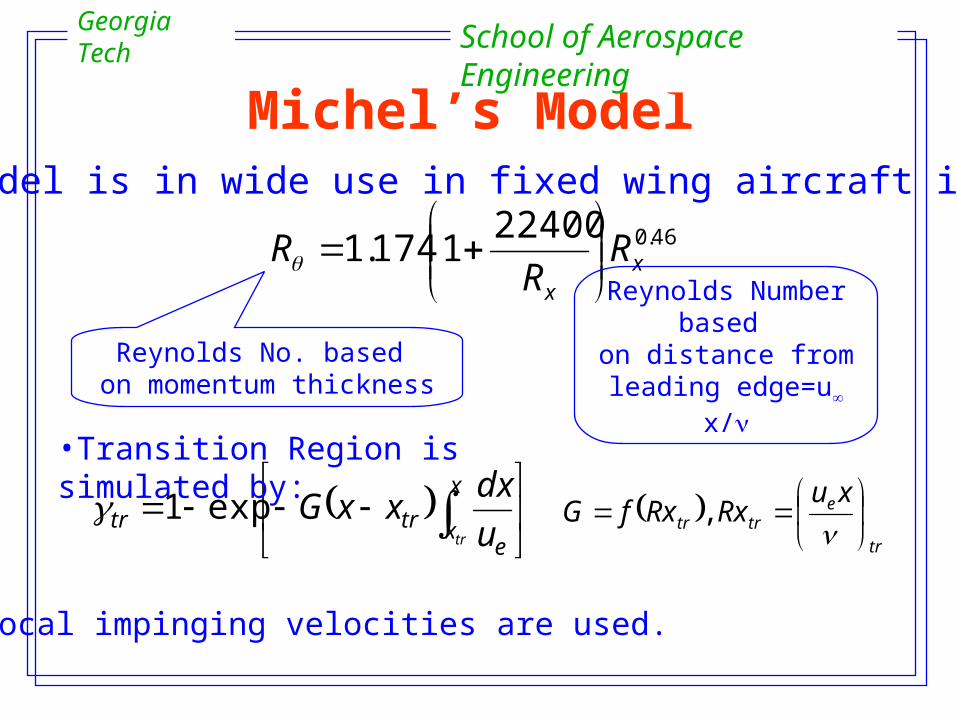
Michel’s Model

46.0224001174.1 x

x

RR

R

This model is in wide use in fixed wing aircraft industry.

Reynolds No. based on momentum thickness

Reynolds Number based on distance from leading

edge=u x/

x

xe

trtrtr u

dxxxGexp1

tr

etrtr

xuRxRxfG

,

•Transition Region is simulated by:


•Local impinging velocities are used.

Vx

Advancing side

Retreating side

vI(r,)

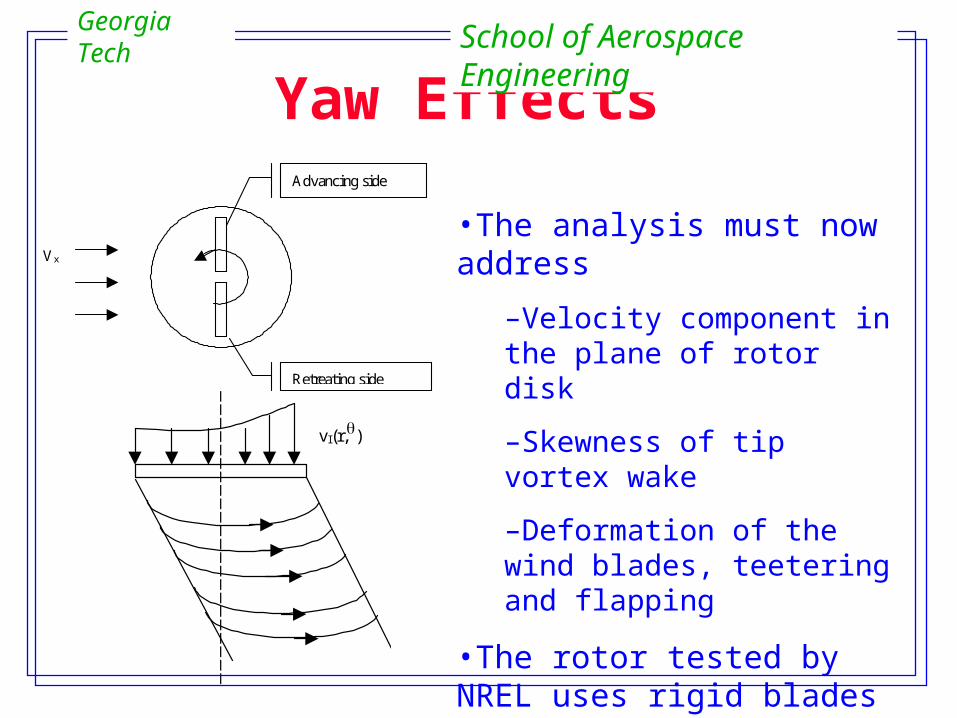
Yaw Effects

•The analysis must now address

–Velocity component in the plane of rotor disk

–Skewness of tip vortex wake

–Deformation of the wind blades, teetering and flapping

•The rotor tested by NREL uses rigid blades


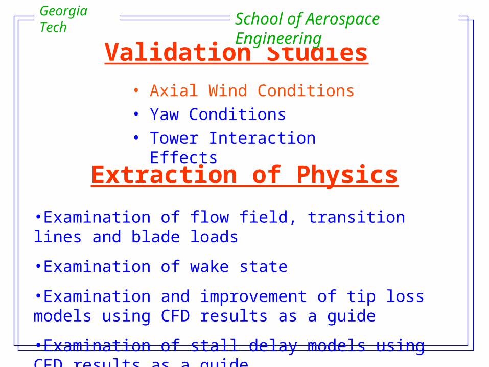
Validation Studies

• Axial Wind Conditions

• Yaw Conditions

• Tower Interaction Effects


Extraction of Physics

•Examination of flow field, transition lines and blade loads

•Examination of wake state

•Examination and improvement of tip loss models using CFD results as a guide

•Examination of stall delay models using CFD results as a guide

Validation Studies (I)

• NREL has collected extensive performance data for three rotor configurations:– A rotor with rectangular planform, untwisted blade and S-809

airfoil sections, called the Phase II Rotor

– A twisted rotor, with rectangular planform and S-809

sections, called the Phase III Rotor

– A two bladed, tapered and twisted rotor, called the Phase VI

Rotor. Best quality measurements (wind tunnel) are available.


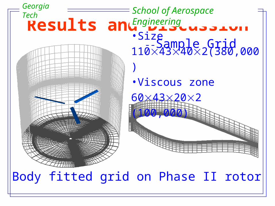
Results and Discussion--Sample Grid

Body fitted grid on Phase II rotor

•Size

11043402(380,000)•Viscous zone 6043202

(100,000)


-10

-5

0

5

10

15

20

0 5 10 15 20 25Wind Speeds[m/s]

Gen

erat

or

Po

wer

[kw

]

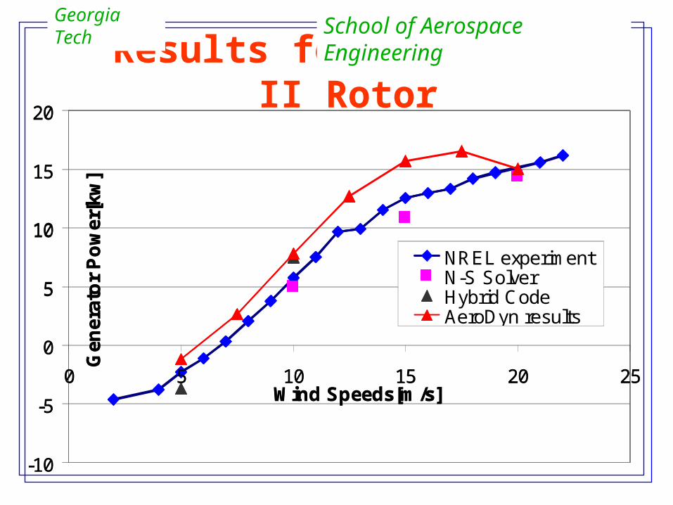
NREL experimentN-S SolverHybrid CodeLifting Line results

-10

-5

0

5

10

15

20

0 5 10 15 20 25Wind Speeds[m/s]

Gen

erat

or

Po

wer

[kw

]

NREL experimentN-S SolverHybrid CodeAeroDyn results

Results for the Phase II Rotor


0

5

10

15

20

0 5 10 15 20

Wind Speed[m/s]

Gen

erat

or

Po

wer

[kw

]

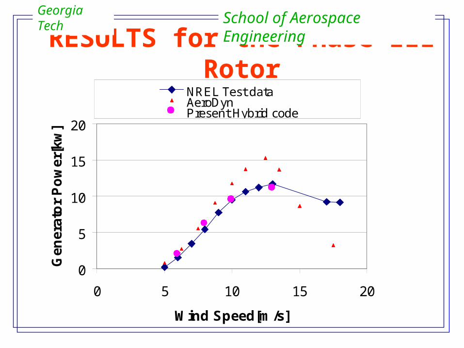
NREL Test dataAeroDynPresent Hybrid code

RESULTS for the Phase III Rotor


The Hybrid Code Converges Rapidly (7 seconds/iteration on a SGI Octane 2 Workstation)

0

4

8

12

16

20

0 1000 2000 3000 4000 5000Iterations of code

Po

we

r(k

w)

6 m/s

10 m/s

8 m/s


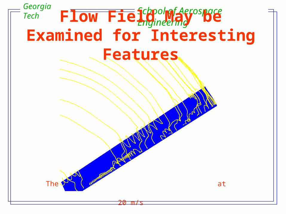
The Upper Surface of the Phase II Rotor at 20 m/s


Flow Field May be Examined for Interesting Features

-3

-2

-1

0

1

2

3

0 2 4 6 8 10 12

0_eqn;Eppler0_eqn; Michel

1_eqn; Eppler1_eqn; Michel

Root Tip

Leading Edge WR

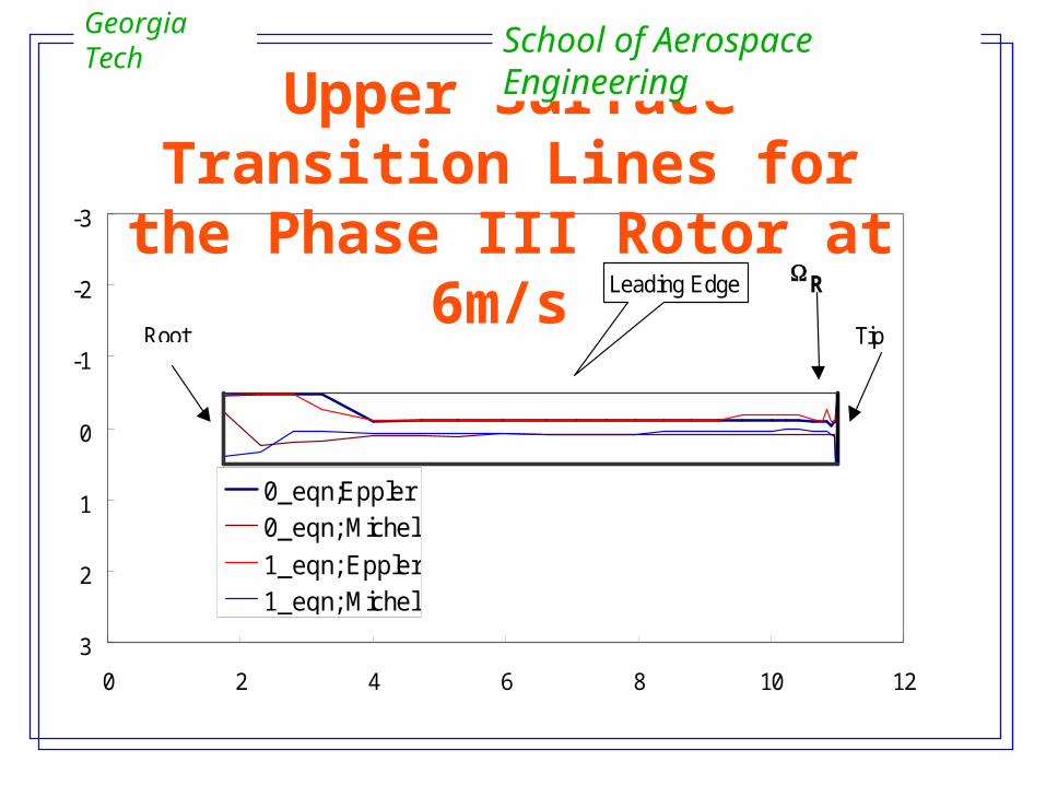
Upper Surface Transition Lines for the Phase III Rotor at 6m/s


-3

-2

-1

0

1

2

3

0 2 4 6 8 10 12

0_eqn;Eppler

0_eqn; Michel

1_eqn; Eppler

1_eqn; Michel

Root Tip

Leading Edge

WR

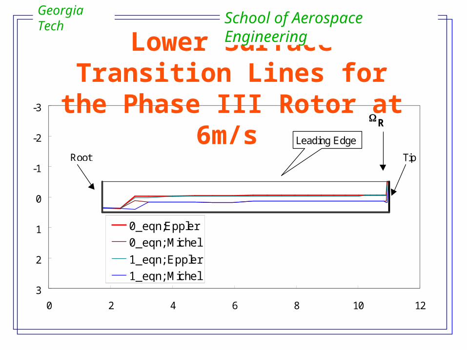
Lower Surface Transition Lines for the Phase III Rotor at 6m/s


Performance of Transition and Turbulence Models

•Eppler’s model predicts a transition location that is slightly upstream of Michel’s predictions, unless if there is a laminar separation bubble.

•On the lower surface, the pressure gradients tend to be more favorable than on the upper side. This leads to a thinner boundary layer and transition aft of the 40% chord.

•The Reynolds number near the root is less than 105. Both models predict that the lower surface flow will remain laminar all the way to the trailing edge, near the root region.

•Transition line location appears insensitive to the turbulence model used.



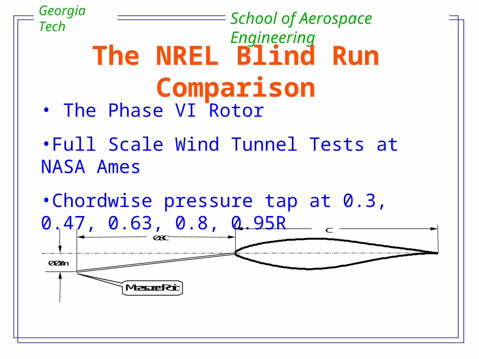
The NREL Blind Run Comparison

• The Phase VI Rotor

•Full Scale Wind Tunnel Tests at NASA Ames

•Chordwise pressure tap at 0.3, 0.47, 0.63, 0.8, 0.95R-0.5

0.5

0.8C

0.03m

C

Measured Point


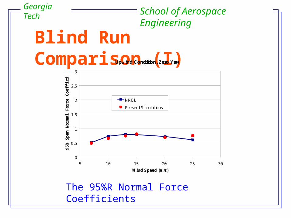
Blind Run Comparison (I)Upwind Condition, Zero Yaw

0

0.5

1

1.5

2

2.5

3

5 10 15 20 25 30

Wind Speed (m/s)

95%

Sp

an N

orm

al F

orc

e C

oef

fici

ent

NREL

Present Simulations

The 95%R Normal Force Coefficients


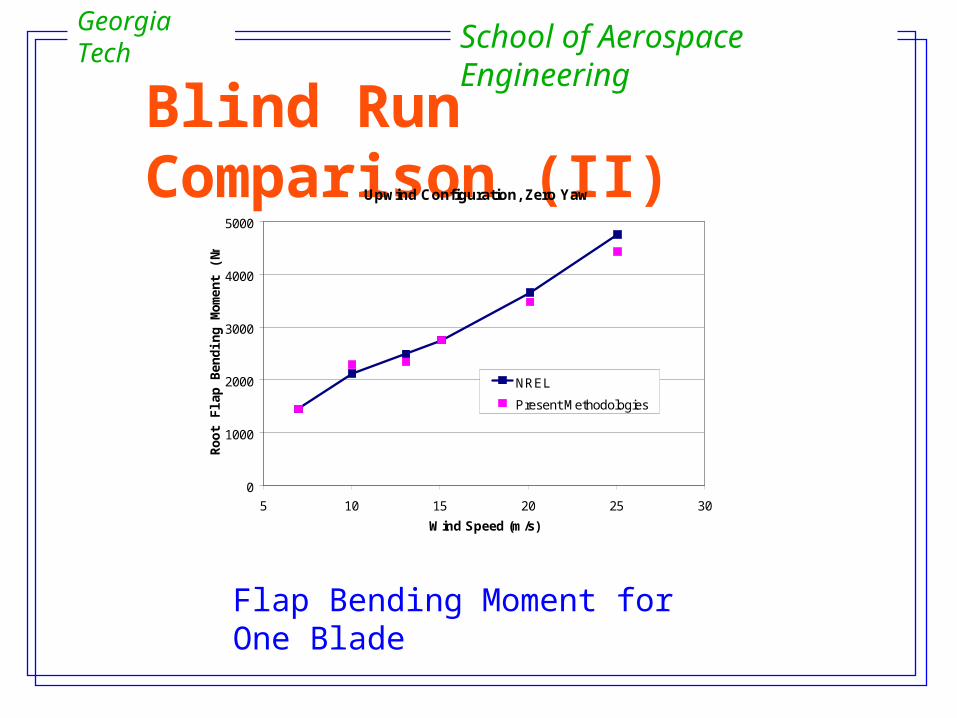
Blind Run Comparison (II)Upwind Configuration, Zero Yaw

0

1000

2000

3000

4000

5000

5 10 15 20 25 30

Wind Speed (m/s)

Ro

ot

Fla

p B

end

ing

Mo

men

t (N

m)

NREL

Present Methodologies

Flap Bending Moment for One Blade


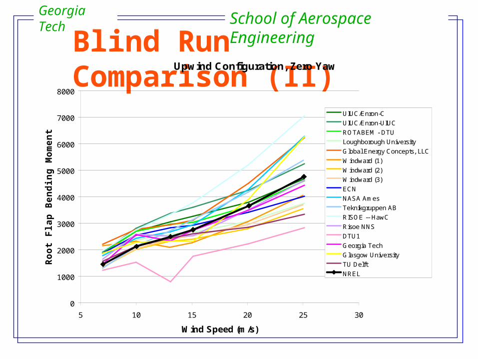
Blind Run Comparison (II)Upwind Configuration, Zero Yaw

0

1000

2000

3000

4000

5000

6000

7000

8000

5 10 15 20 25 30

Wind Speed (m/s)

Ro

ot

Fla

p B

en

din

g M

om

en

t (N

m)

UIUC/Enron-C

UIUC/Enron-UIUC

ROTABEM - DTU

Loughborough University

Global Energy Concepts, LLC

Windward (1)

Windward (2)

Windward (3)

ECN

NASA Ames

Teknikgruppen AB

RISOE -- HawC

Risoe NNS

DTU1

Georgia Tech

Glasgow University

TU Delft

NREL


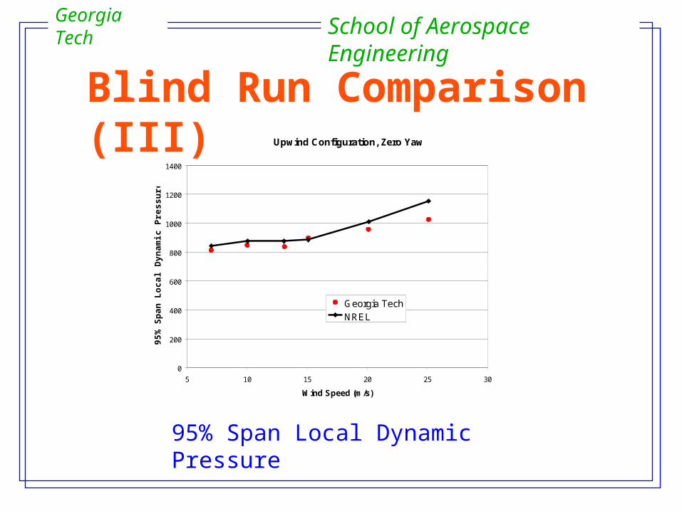
Blind Run Comparison (III)Upwind Configuration, Zero Yaw

0

200

400

600

800

1000

1200

1400

5 10 15 20 25 30

Wind Speed (m/s)

95

% S

pa

n L

oc

al

Dy

na

mic

Pre

ss

ure

(P

a)

Georgia TechNREL

95% Span Local Dynamic Pressure

Validation Studies


• Yaw Conditions








Yaw Simulations


•Field data is often unreliable because of constantly shifting wind conditions.

•Phase VI data is highly reliable, but unfortunately was not available till towards the end of this research.

•For these reasons, the present simulations have not been validated in the strictest sense, but do give useful insight into yaw effects.

8.0

8.5

9.0

9.5

10.0

10.5

11.0

11.5

0 2 4 6 8 10 12 14 16

Time(sec)

Me

asu

red

Win

d S

pe

ed

Inflow wind(3)inflow wind(4)

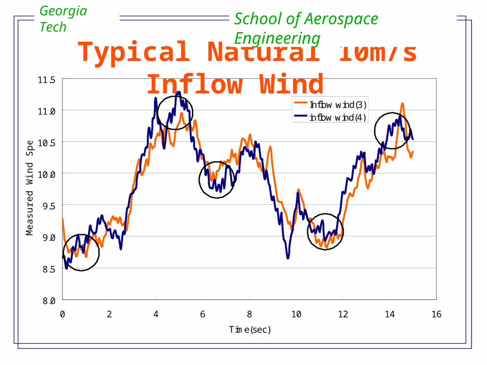
Typical Natural 10m/s Inflow Wind


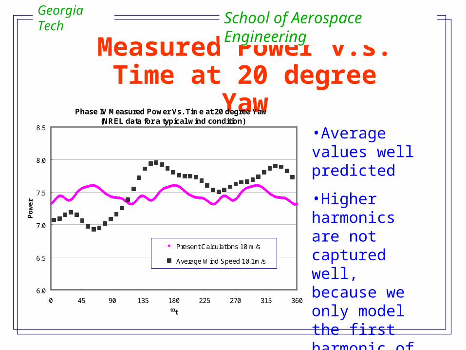
Measured Power v.s. Time at 20 degree Yaw


Phase IV Measured Power Vs. Time at 20 degree Yaw (NREL data for a typical wind condition)

6.0

6.5

7.0

7.5

8.0

8.5

0 45 90 135 180 225 270 315 360

t

Po

we

r

Present Calculations 10 m/s

Average Wind Speed 10.1m/s

•Average values well predicted

•Higher harmonics are not captured well, because we only model the first harmonic of the wind.

Validation Studies


• Yaw Conditions








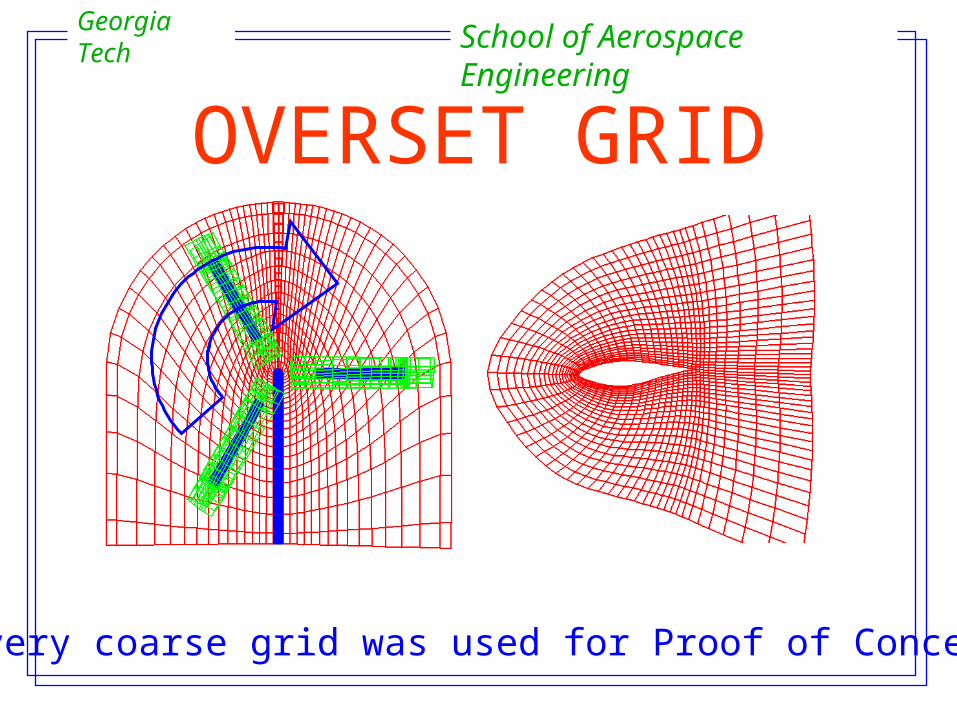
OVERSET GRID

A very coarse grid was used for Proof of Concept


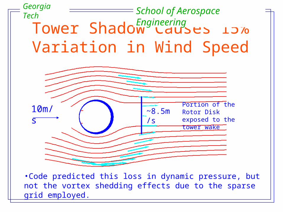
Portion of the Rotor Disk exposed to the tower wake

Tower Shadow Causes 15% Variation in Wind Speed


10m/s ~8.5m/s

•Code predicted this loss in dynamic pressure, but not the vortex shedding effects due to the sparse grid employed.

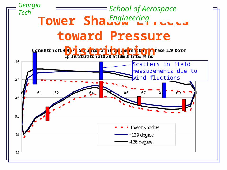
Correlation of CHIMERA Simulation with Measurement for the Phase III/IV RotorCp Distributation at 0.8R at 10m/s Inflow Wind

-1.0

-0.5

0.0

0.5

1.0

1.5

0 0.1 0.2 0.3 0.4 0.5 0.6 0.7 0.8 0.9 1

Tower Shadow

+120 degree

-120 degree

Tower Shadow Effects toward Pressure Distribution


Scatters in field measurements due to wind fluctions

Validation Studies


• Yaw Conditions








Study of Wind Turbine States

•Wind Turbine States includes: Propeller, zero-slip,windmill, turbulent windmill, vortex ring, and propeller brake states.

•The present method models all these states well.

•Ignoring transition from one state to another will lead to incorrect performance predictions.


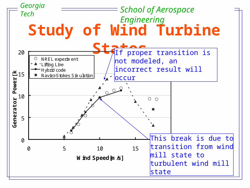
Study of Wind Turbine States

0

5

10

15

20

0 5 10 15 20

Wind Speed[m/s]

Gen

erat

or

Po

wer

[kw

]

NREL experimentLifting LineHybrid codeNavier-Stokes Simulation

This break is due to transition from wind mill state to turbulent wind mill state

If proper transition is not modeled, an incorrect result will occur


Validation Studies


• Yaw Conditions








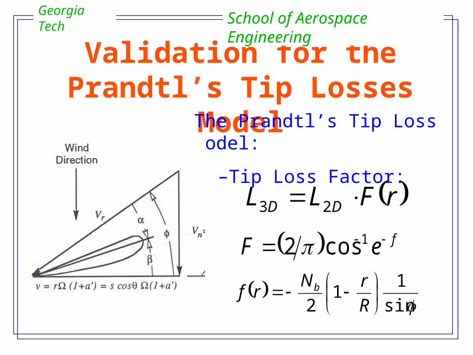
Validation for the Prandtl’s Tip Losses Model

feF 1cos2

The Prandtl’s Tip Loss Model:

–Tip Loss Factor:

sin

11

2

R

rNrf b

rFLL DD 23


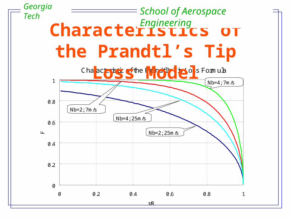
Characteristic of the Prandtl's Tip Loss Formula

0

0.2

0.4

0.6

0.8

1

0 0.2 0.4 0.6 0.8 1

r/R

F Nb=2; 25m/s

Nb=4; 25m/s

Nb=4; 7m/s

Nb=2; 7m/s

Characteristics of the Prandtl’s Tip Loss Model


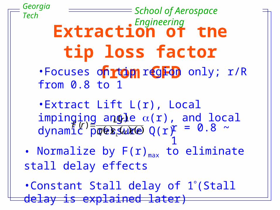
Extraction of the tip loss factor from CFD

•Focuses on tip region only; r/R from 0.8 to 1

•Extract Lift L(r), Local impinging angle (r), and local dynamic pressure Q(r)

rccrQ

rLrF

L )( r = 0.8 ~ 1

• Normalize by F(r)max to eliminate stall delay effects

•Constant Stall delay of 1(Stall delay is explained later)


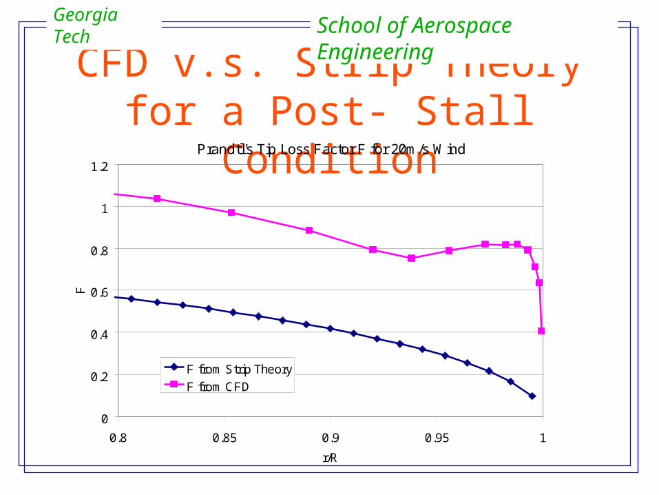
CFD v.s. Strip Theory for a Post- Stall Condition

Prandtl's Tip Loss Factor F for 20m/s Wind

0

0.2

0.4

0.6

0.8

1

1.2

0.8 0.85 0.9 0.95 1

r/R

F

F from Strip Theory

F from CFD


CFD v.s. Strip Theory for Pre-Stall Condition (I)

Prandtl's Tip Loss Factor F for 7m/s Wind

0

0.2

0.4

0.6

0.8

1

0.8 0.85 0.9 0.95 1

r/R

F

F from CFD

F from Strip Theory


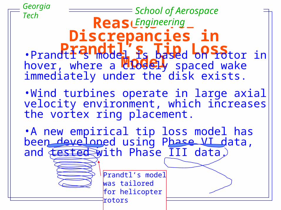
Reasons for Discrepancies in Prandtl’s Tip Loss Model

•Prandtl’s model is based on rotor in hover, where a closely spaced wake immediately under the disk exists.

•Wind turbines operate in large axial velocity environment, which increases the vortex ring placement.

•A new empirical tip loss model has been developed using Phase VI data, and tested with Phase III data.

Prandtl’s model was tailored for helicopter rotors


-1500

-1000

-500

0

500

1000

1500

2000

0 5 10 15 20 25

wind speed

torq

ue

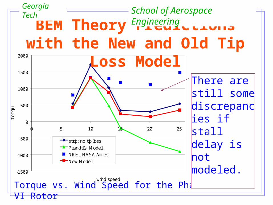
strip; no tip loss

Prandtl's Model

NREL NASA Ames

New Model

BEM Theory Predictions with the New and Old Tip Loss Model

Torque vs. Wind Speed for the Phase VI Rotor

There are still some discrepancies if stall delay is not modeled.


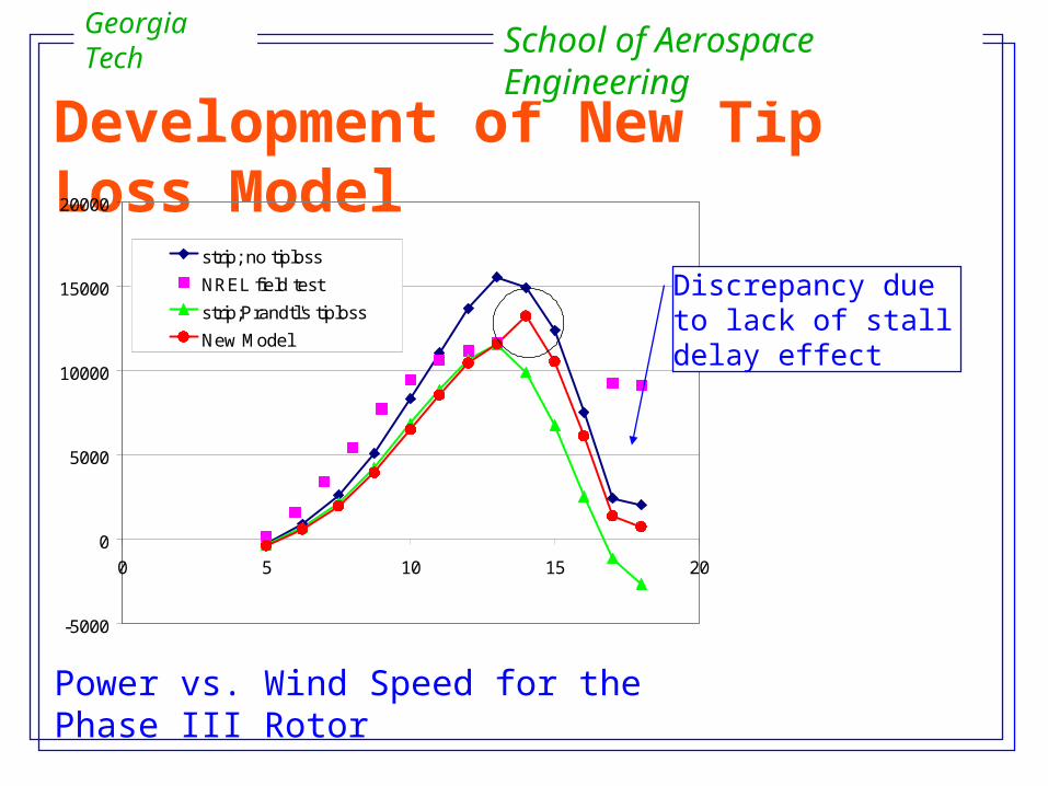
Development of New Tip Loss Model

Power vs. Wind Speed for the Phase III Rotor

-5000

0

5000

10000

15000

20000

0 5 10 15 20

strip; no tiploss

NREL field test

strip;Prandtl's tiploss

New Model

Discrepancy due to lack of stall delay effect


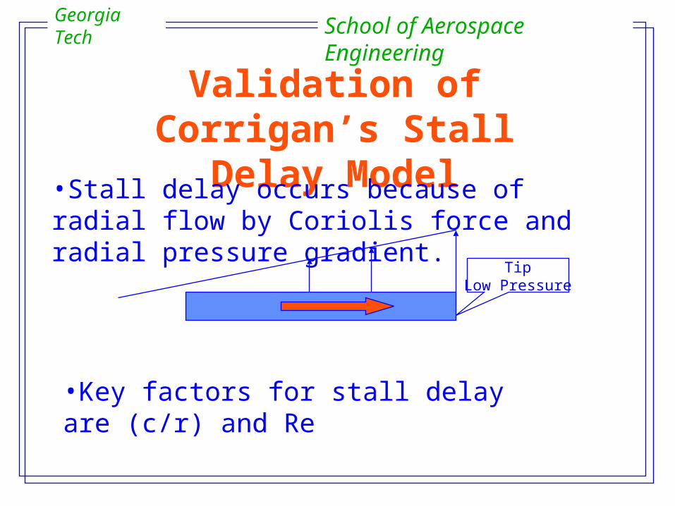
Validation of Corrigan’s Stall Delay Model

•Stall delay occurs because of radial flow by Coriolis force and radial pressure gradient.

TipLow Pressure

•Key factors for stall delay are (c/r) and Re


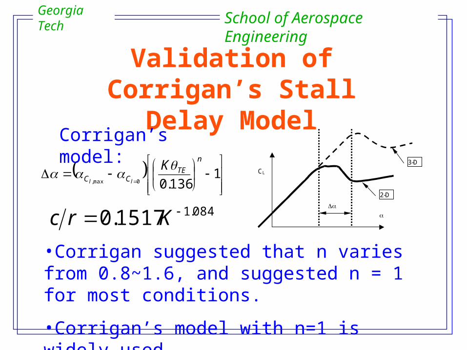
Validation of Corrigan’s Stall Delay Model

2-D

3-DCL

1

136.00max,

n

TECC

Kll

084.11517.0 Krc

Corrigan’s model:

•Corrigan suggested that n varies from 0.8~1.6, and suggested n = 1 for most conditions.

•Corrigan’s model with n=1 is widely used.


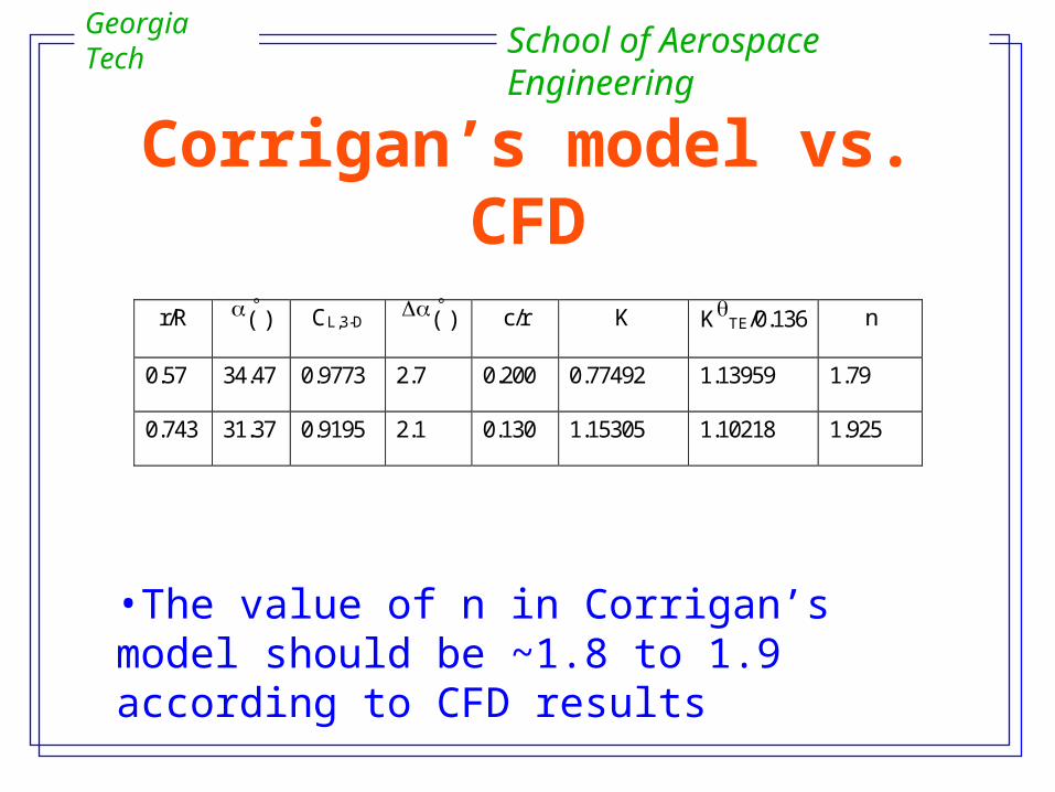
Corrigan’s model vs. CFD

•The value of n in Corrigan’s model should be ~1.8 to 1.9 according to CFD results

r/R ( ) CL,3-D( ) c/r K KTE/0.136 n

0.57 34.47 0.9773 2.7 0.200 0.77492 1.13959 1.79

0.743 31.37 0.9195 2.1 0.130 1.15305 1.10218 1.925


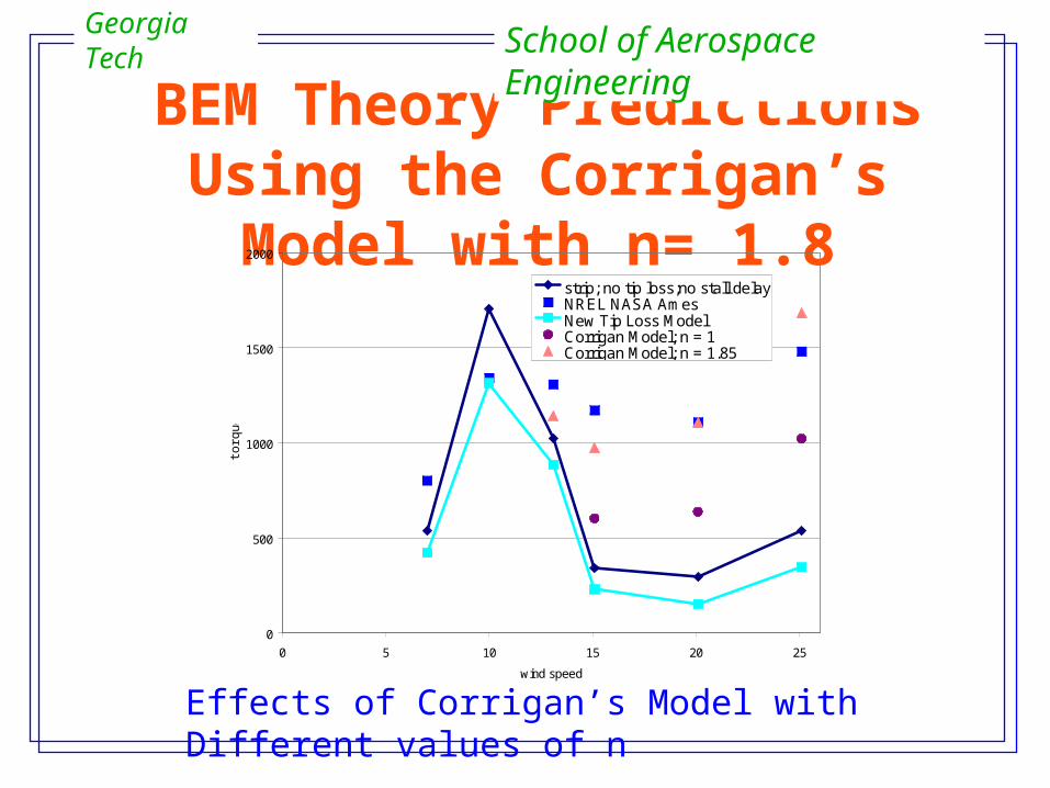
BEM Theory Predictions Using the Corrigan’s Model with n= 1.8

0

500

1000

1500

2000

0 5 10 15 20 25

wind speed

torq

ue

strip; no tip loss;no stall delayNREL NASA AmesNew Tip Loss ModelCorrigan Model; n = 1Corrigan Model; n = 1.85

Effects of Corrigan’s Model with Different values of n


Conclusions (I)

•The Hybrid methodology is an efficient means of studying

the HAWT flow phenomena for both axial and yaw

conditions.

•The Spalart-Allmaras model, a one-equation turbulence

model, predicts higher turbulence viscosity than the

Baldwin-Lomax turbulence model. As a consequence the

Spalart-Allmaras model predicts slightly lower power

values. Nevertheless, both models yield power predictions

that are well within the uncertainties associated with the

measurements.


Conclusions(II)•The Eppler’s transition model and the Michel’s transition model in the present methodology both give comparable transition locations. The Eppler’s model assumes that transition will occur if there is a laminar separation bubble at the leading edge. Based on this physical consideration, Eppler’s model is considered to be superior to Michel’s model.

•Wind turbine states profoundly affects the power estimates. Proper transition of the wake geometry from one state to the next, as the wind speed increases, is found to be essential to accurately predicting the generated power.


Conclusions(III)•The present simulations for rotors operating in yaw conditions reveal that presence of Nb-per revolution, 2Nb-per-rev, and higher harmonic fluctuations in the loads, where Nb is the number of blades. Accurate prediction of these higher harmonics is important for fatigue life estimates.

•The present simulations suggest a very small reduction in power due to tower shadow effects. If one is interested in power estimates, it is not necessary to include tower effects. However, the tower wake can trigger dynamic stall, which will persist over a larger potion of the rotor disk. Tower effects must be studied if these factors, which contribute to fatigue, are important.


Recommendation(I)

•The present method is quite efficient ( ~ 4 hours on a Linux

system). Further efficiency gains are possible using multigrid,

local time stepping, parallel/distributed computing, etc. These

options must be explored.

•Further validation of the present method using the high quality

Phase VI Rotor data is recommended.

•The proposed wake state models can and should be

implemented in industry methods such as YawDyn, to correctly

model the breaks in the Power vs. Wind Speed Curve.


Recommendation(II)

•The proposed tip loss model (based on curve-fit of Phase III

rotor results), and the stall delay model (n = 1.8) should be

further tested, using Phase VI and other wind tunnel data.

•The present study relied on power measurement, a global

quantity. Flow details such as velocity, vorticity, turbulence

load etc, must be studied and improving using Phase VI data.


Documents

Computational Studies of Horizontal Axis Wind Turbines Ph.D. Oral Defense Presented By Guanpeng Xu Advisor: Dr. L Sankar School of Aerospace Engineering