Computational Simulations and Experiments on Vibration Control of a Flexible Two-link ... · 2015-07-09 · the equations of motion of a flexible two-link system, ... calculated results

Abstract— The purposes of this research are to formulate

the equations of motion of a flexible two-link system, to develop

computational codes by a finite-element method in order to

perform dynamics simulations with vibration control, to

propose an effective control scheme and to confirm the

calculated results by experiments of a flexible two-link

manipulator. The system used in this paper consists of two

aluminum beams as flexible links, two clamp-parts, two servo

motors to rotate the links and a piezoelectric actuator to control

vibration. Computational codes on time history responses, FFT

(Fast Fourier Transform) processing and eigenvalues -

eigenvectors analysis were developed to calculate the dynamic

behavior of the links. Furthermore, a control scheme using a

piezoelectric actuator was designed to suppress the vibration. A

proportional-derivative (PD) control was designed and

demonstrated its performances. The system and the proposed

control scheme were confirmed through experiments. The

calculated and experimental results revealed that the vibration

of the flexible two-link manipulator can be controlled

effectively.

Index Terms—Finite-element method, flexible manipulator,

piezoelectric actuator, vibration control.

I. INTRODUCTION

MPLOYMENT of flexible link manipulator is

recommended in the space and industrial applications in

order to accomplish high performance requirements such as

high-speed besides safe operation, increasing of positioning

accuracy and lower energy consumption, namely less weight.

However, it is not usually easy to control a flexible

manipulator because of its inheriting flexibility. Deformation

of the flexible manipulator when it is operated must be

considered by any control. Its controller system should be

dealt with not only its motion but also vibration due to the

flexibility of the link.

In the past few decades, a number of modeling methods

and control strategies using piezoelectric actuators to deal

with the vibration problem have been investigated by

researchers [1 – 10]. Nishidome and Kajiwara [1]

investigated a way to enhance performances of motion and

vibration of a flexible-link mechanism. They used a modeling

Manuscript received April 30, 2015; revised May 21, 2015.

Every author is with Mechanical Engineering Course, Graduate School of Science and Engineering, Ehime University, 3 Bunkyo-cho, Matsuyama

790-8577, Japan. (e-mail: [email protected],

[email protected], [email protected], [email protected] ).

The first author is also with Center for Mechatronics and Control System, Mechanical Engineering Department, State Polytechnic of Ujung Pandang,

Jl. Perintis Kemerdekaan KM 10 Makassar, 90-245, Indonesia.

method based on modal analysis using the finite-element

method. The model was described as a state space form.

Their control system was constructed with a designed

dynamic compensator based on the mixed of H2/H∞. They

recommended separating the motion and vibration controls of

the system. Yavus Yaman et al [2] and Kircali et al [3]

studied an active vibration control technique on aluminum

beam modeled in cantilevered configuration. The studies

used the ANSYS package program for modeling. They

investigated the effect of element selection in finite-element

modeling. The model was reduced to state space form

suitable for application of H∞ [2] and spatial H∞ [3]

controllers to suppress vibration of the beam. They showed

the effectiveness of their techniques through simulation.

Zhang et al [4] has studied a flexible piezoelectric cantilever

beam. The model of the beam using finite-elements was built

by ANSYS application. Based on the Linear Quadratic Gauss

(LQG) control method, they introduced a procedure to

suppress the vibration of the beam with the piezoelectric

sensors and actuators were symmetrically collocated on both

sides of the beam. Their simulation results showed the

effectiveness of the method. Gurses et al [5] investigated

vibration control of a flexible single-link manipulator using

three piezoelectric actuators. The dynamic modeling of the

link had been presented using Euler-Bernoulli beam theory.

Composite linear and angular velocity feedback controls

were introduced to suppress the vibration. Their simulation

and experimental results showed the effectiveness of the

controllers. Xu and Koko [6] studied finite-element analysis

and designed controller for flexible structures using

piezoelectric material as actuators and sensors. They used a

commercial finite-element code for modeling and completed

with an optimal active vibration control in state space form.

The effectiveness of the control method was confirmed

through simulations. Kusculuoglu et al [7] had used a

piezoelectric actuator for excitation and control vibrations of

a beam. The beam and actuator were modeled using

Timoshenko beam theory. An optimized vibration absorber

using an electrical resistive-inductive shun circuit on the

actuator was used as a passive controller. The effectiveness

of results was shown by simulations and experiment.

Furthermore, Hewit et al [8] used the Active-force (AF)

control for deformation and disturbance attenuation of a

flexible manipulator. Then, a PD control was used for

trajectory tracking of the flexible manipulator. They used a

motor as an actuator. Modeling of the manipulator was done

using virtual link coordinate system (VLCS). Their

simulation results had shown that the proposed control could

cancel the disturbance satisfactorily. Tavakolvour et al [9]

investigated the AF control application for a flexible thin

plate. Modeling of their system was done using

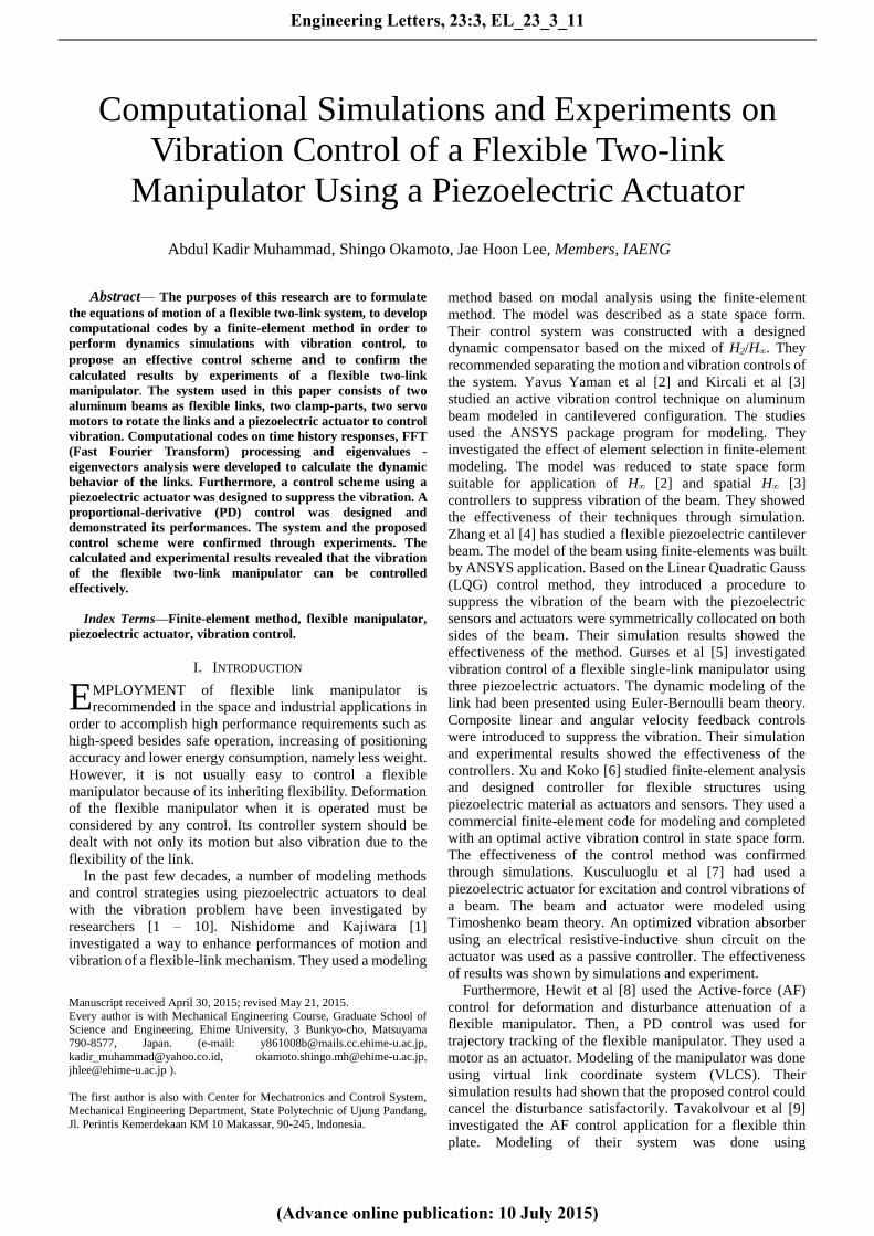
Computational Simulations and Experiments on

Vibration Control of a Flexible Two-link

Manipulator Using a Piezoelectric Actuator

Abdul Kadir Muhammad, Shingo Okamoto, Jae Hoon Lee, Members, IAENG

E

Engineering Letters, 23:3, EL_23_3_11

(Advance online publication: 10 July 2015)

______________________________________________________________________________________

mailto:[email protected]



finite-difference method. Their calculated results showed the

effectiveness of the proposed controller to reduce vibration of

the plate. Tavakolvour and Mailah [10] studied the AF

control application for a flexible beam with an

electromagnetic actuator. Modeling of the beam was done

using finite-difference method. The effectiveness of the

proposed controller was confirmed through simulation and

experiment.

In the recent two years, Muhammad et al [11 – 15] have

actively studied vibration control on a flexible single-link

manipulator with a piezoelectric actuator using finite-element

method. Model of the single-link and the piezolecetric

actuator was built using one-dimensional and two-node

elements. They introduced a simple and effective control

scheme with the actuator using proportional (P), PD and AF

controls strategies. The effectivenesses of the proposed

control scheme and strategies were shown through

simulations and experiments.

The purposes of this research are to derive the equations of

motion of a flexible two-link system by a finite-element

method, to develop computational codes in order to perform

dynamics simulations with vibration control and to propose

an effective control scheme of a flexible two-link

manipulator.

The flexible two-link manipulator used in this paper

consists of two aluminum beams as flexible links, two

aluminum clamp-parts, two servo motors to rotate the links

and a piezoelectric actuator to control vibration.

Computational codes on time history responses, FFT (Fast

Fourier Transform) processing and eigenvalues -

eigenvectors analysis were developed to calculate the

dynamic behavior of the links. Finally, a PD controller was

designed to suppress the vibration. It was done by adding

bending moments generated by the piezoelectric actuators to

the two-link system.

II. FORMULATION BY FINITE-ELEMENT METHOD

The links have been discretized by finite-elements. Every

finite-element (Element i-th) has two nodes namely Node i

and Node (i+1). Every node (Node i) has two degrees of

freedom [11 – 15], namely the lateral deformation vi(x,t), and

the rotational angle ψi(x,t) . The length, the cross-sectional

area and the area moment of inertia around z-axis of every

element are denoted by li, Si and Izi respectively. Mechanical

properties of every element are denoted as Young’s modulus

Ei and mass density ρi.

A. Kinematic

Figure 1 shows the position vectors rp1 and rp2 of arbitrary

points P1 and P2 on Link 1 and Link 2 in the global and

rotating coordinate frames. Let the links as flexible beams

have a motion that is confined in the horizontal plane as

shown in Fig. 1. The O – XY frame is the global coordinate

frame with Z-axis is fixed. Furthermore, o1 – x1y1 and o2 –

x2y2 are the rotating coordinate frames fixed to the root of

Link 1 and Link 2, respectively (z1-axis and z2-axis are fixed).

The unit vectors in X, Y, x1, y1, x2 and y2 axes are denoted by I,

J, i1, j1, i2 and j2, respectively. The first motor is installed on

the root of the Link 1. The second motor that treated as a

concentrated mass is installed in the root of the Link 2. The

rotational angles of the first and second motor when the links

rotate are denoted by θ1(t) and θ2(t). Length of Link 1 is

donated by L1. Lateral deformation of the arbitrary points P1

and P2 in the first and the second links are donated by vp1 and

O-XY : Global coordinate frame o1-x1y1 : Rotating coordinate frame fixed to Link 1

o2-x2y2 : Rotating coordinate frame fixed to Link 2

rp1, rp2 : Position vectors of the arbitrary points p1 and p2 in the O-XY θ1 : Rotational angle of the first motor

θ2 : Rotational angle of the second motor

Xp1, Xp2 : Coordinates of the arbitrary points p1 and p2 in the X-axis of the O-XY

Yp1, Yp2 : Coordinates of the arbitrary points p1 and p2 in the Y-axis of the

O-XY νp1 : Lateral deformation of the arbitrary point p1 on Link 1 in the

o1-x1y1

νp2 : Lateral deformation of the arbitrary point p2 on Link 2 in the o2-x2y2

ψe : Rotational angle of the end-point of Link 1

ve : Lateral deformation of the end-point of Link 1 L1 : Length of Link 1

Fig. 1. Position vectors of arbitrary points P1 and P2 in the global and rotating coordinate frames

vp2, respectively. Lateral deformation and rotational angel of

the end-point of the first link are donated by ve and ψe,

respectively. The position vectors rp1 and rp2 of the arbitrary

points P1 and P2 at time t = t, measured in the O – XY frame

shown in Fig. 1 are expressed by

JIr ),,,(),,,( 111111111 tvxYtvxX ppppp (1)

Ir ),,,,,,( 221222 tvvxX peepp

J),,,,,,( 22122 tvvxY peep (2)

Where

)(sin),()(cos 111111 ttxvtxX pp (3) (2) Error! Reference source not found.

)(cos),()(sin 111111 ttxvtxY pp (4)

)(sin),()(cos 11112 ttxvtLX ep

)(),()(cos 2112 ttxtx e

)(),()(sin),( 21122 ttxttxv ep (5)

)(cos),()(sin 11112 ttxvtLY ep

)(),()(sin 2112 ttxtx e

)(),()(cos),( 21122 ttxttxv ep (6)

The velocity vectors of the arbitrary points P1 and P2 at time t

= t, shown in Fig.1 are expressed by

JIr ),,,,,(),,,,,( 1111111111111 tvvxYtvvxX ppppppp

(7)



______________________________________________________________________________________

Ir ),,,,,,,,,,,( 222121222 tvvvvxX peepeepp

J),,,,,,,,,,,( 22212121 tvvvvxY peepeep

(8)

B. Finite-element Method

Figure 2 shows the element coordinate frame of Element i,

and an arbitrary point P on Element i. Here, there are four

boundary conditions together at nodes i and (i+1) when the

one-dimensional and two-node element is used. The four

boundary conditions are expressed as nodal vector as follow

Tiiiii vv 11 δ

(9)

Then, the hypothesized deformation has four constants as

follows [16]

3

42

321 iiii xaxaxaav (10)

where xi is position coordinate of the arbitrary point P in the

xi-axis of the element coordinate frame.

Then, the relation between the lateral deformation vi and the

rotational angle ψi of the Node i is given by

i

ii

x

v

(11)

Moreover, from mechanics of materials, the strain of Node i

can be defined by

2

2

i

iii

x

vy

(12)

where yi is position coordinate of the arbitrary point P in the

yi-axis of the element coordinate frame.

oi – xi yi: Element coordinate frame of the Element i

Fig. 2. Element coordinate frame of the Element i

C. Equations of motion

Equations of motion of Element i-th on Link 1 and Link 2

are respectively given by

iiiiiiii fδMKδCδM 12

1 (13)

ieeee

ieeeie

iieiiiii

vLv

vvL

g

gf

δMKδCδM

2212

111

22

11121

2

21

sin32

1

cos

(14)

where Mi, Ci, and Ki, are the mass matrix, damping matrix,

stiffness matrix of Element i on Link 1 and Link 2. Vectors of

fi and gi are the excitation vectors on Link 1 and Link 2. The

representation of the matrices and the vector of fi can be

found in [11] and [13]. The vector of gi can be defined by

Tii

iiii ll

lS6156

12

g (15)

Finally, the equations of motion of Link 1 and Link 2 with

n elements considering the boundary conditions is

respectively given by

nnnnnnnn fδMKδCδM 12

1 (16)

neeee

neeene

nnennnnn

vLv

vvL

g

gf

δMKδCδM

2212

111

22

11121

2

21

sin32

1

cos

(17)

III. VALIDATION OF FORMULATION AND COMPUTATIONAL

CODES

A. Experimental Model

Figure 3 shows the experimental model of the flexible

two-link manipulator. The flexible manipulator consists of

two flexible aluminum beams, two clamp-parts, two servo

motors and the base. Link 1 and Link 2 are attached to the

first and second motors through the clamp-parts. Link 1 and

Link 2 are connected through the second motor. Two strain

gages are bonded to the position of 0.11 [m] and 0.38 [m]

from the origin of the two-link system. The first motor is

mounted to the base. In the experiments, the motors were

operated by an independent motion controller.

Fig. 3. Experimental model of the flexible two-link manipulator

B. Computational Models

In this research, we defined and used three types of

computational models of the flexible two-link manipulator.

Model A

A model of only a two-link manipulator was used as Model

A. Figure 4.a shows Model A. The links and the clamp-parts

were discretized by 35 elements. Two strain gages are



______________________________________________________________________________________

bonded to the position of Node 6 and Node 22 of the two-link

(0.11 [m] and 0.38 [m] from the link’s origin), respectively.

Model B

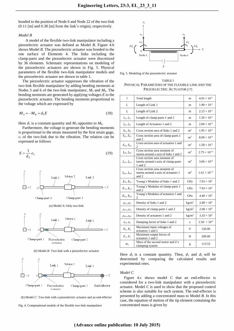
A model of the flexible two-link manipulator including a

piezoelectric actuator was defined as Model B. Figure 4.b

shows Model B. The piezoelectric actuator was bonded to the

one surface of Elements 4. The links including the

clamp-parts and the piezoelectric actuator were discretized

by 36 elements. Schematic representations on modeling of

the piezoelectric actuators are shown in Fig. 5. Physical

parameters of the flexible two-link manipulator models and

the piezoelectric actuator are shown in table 1.

The piezoelectric actuator suppresses the vibration of the

two-link flexible manipulator by adding bending moments at

Nodes 3 and 6 of the two-link manipulator, M3 and M6. The

bending moments are generated by applying voltages E to the

piezoelectric actuator. The bending moments proportional to

the voltage which are expressed by

EdMM 163

(18)

Here d1 is a constant quantity and M3 opposites to M6.

Furthermore, the voltage to generate the bending moments

is proportional to the strain measured by the first strain gage,

ε1 of the two-link due to the vibration. The relation can be

expressed as follows

12

1

dE

(19)

(a) Model A: Only two-link

(b) Model B: Two-link with a piezoelectric actuator

(b) Model C: Two-link with a piezoelectric actuator and an end-effector

Fig. 4. Computational models of the flexible two-link manipulator

Fig. 5. Modeling of the piezoelectric actuator

TABLE I

PHYSICAL PARAMETERS OF THE FLEXIBLE LINK AND THE

PIEZOELECTRIC ACTUATOR [17]

l Total length m 4.05 × 10-1

l1 Length of Link 1 m 1.90 × 10-1

l2 Length of Link 2 m 2.15 × 10-1

lc1, lc2 Length of clamp-parts 1 and 2 m 1.50 × 10-2

la1, la2 Length of Actuators 1 and 2 m 2.00 × 10-2

Sl1, Sl2 Cross section area of links 1 and 2 m2 1.95 × 10-5

Sc1, Sc2

Cross section area of clamp-parts 1

and 2 m2 8.09 × 10-4

Sa1, Sa2 Cross section area of actuators 1 and 2

m2 1.58 × 10-5

Izl1, Izl2 Cross section area moment of

inertia around z-axis of links 1 and 2 m4 2.75 × 10-12

Izc1, Izc2 Cross section area moment of inertia around z-axis of clamp-parts

1 and 2

m4 3.06 × 10-8

Iza1, Iza2 Cross section area moment of inertia around z-axis of actuators 1

and 2

m4 1.61 × 10-11

El1, El2 Young’s Modulus of links 1 and 2 GPa 7.03 × 101

Ec1, Ec2 Young’s Modulus of clamp-parts 1

and 2 GPa 7.03 × 101

Ea1, Ea2 Young’s Modulus of actuators 1 and 2

GPa 4.40 × 101

ρl1, ρl2 Density of links 1 and 2 kg/m3 2.68 × 103

ρc1, ρc2 Density of clamp-parts 1 and 2 kg/m3 2.68 × 103

ρa1, ρa2 Density of actuators 1 and 2 kg/m3 3.33 × 103

α1, α2 Damping factor of links 1 and 2 s 2.50 × 10-4

E1, E2 Maximum input voltages of

actuators 1 and 2 V 150.00

F1, F2 Maximum output forces of

actuators 1 and 2 N 200.00

m2 Mass of the second motor and it’s

clamping system g 113.53

Here d2 is a constant quantity. Then, d1 and d2 will be

determined by comparing the calculated results and

experimental ones.

Model C

Figure 4.c shows model C that an end-effector is

considered for a two-link manipulator with a piezoelectric

actuator. Model C is used to show that the proposed control

scheme is also suitable for such system. The end-effector is

presented by adding a concentrated mass to Model B. In this

case, the equation of motion of the tip element containing the

concentrated mass is given by



______________________________________________________________________________________

icmieeee

icmieee

icmie

iicmiei

iiiicmi

vLv

vvL

gg

gg

ff

δMMK

δCδMM

2212

111

22

111

21

2

21

sin32

1

cos

(20)

where the vectors of ficm and gicm are respectively given by

Tiicicm llm 000 1 f

(21)

T

cicm m 0100 g (22)

and the concentrated mass matrix Micm can be expressed as

0000

000

0000

0000

i

cicm

mM (23)

where mc is the mass of the concentrated mass.

C. Time History Responses of Free Vibration

Experiment on free vibration was conducted using an

impulse force as an external one. Figure 6 shows the

experimental time history response of strains, εe on the free

vibration at the same position in the calculation (0.11 [m]

from the origin of the two-link system). Furthermore, the

computational codes on time history response of Model A

were developed. Figure 7 shows the calculated strains at

Node 6 of Model A under the impulse force.

0 5 10 15 20-300

-200

-100

0

100

200

300

Fig. 6. Experimental time history response of strains on free vibration of the

flexible two-link at 0.11 [m] from the origin of the two-link

0 5 10 15 20-300

-200

-100

0

100

200

300

Fig. 7. Calculated time history response of strains on free vibration at

Node 6 of Model A

D. Fast Fourier Transform (FFT) Processing

Both the experimental and calculated time history

responses on free vibration were transferred by FFT

processing to find their frequencies.

0 10 20 30 40 502

4

6

8

10

12

141.79 Hz

Fig. 8. Experimental natural frequency of the flexible two-link

0 25 50 75 1002

4

6

8

10

12

14 1.80 Hz

8.95 Hz

Fig. 9. Calculated natural frequencies of Model A

Figures 8 and 9 show the experimental and calculated

natural frequencies of the flexible two-link manipulator,

respectively. The first experimental natural frequency, 1.79

[Hz] agreed with the calculated one, 1.80 [Hz]. The second

experimental natural frequency could not be measured.

However, it could be obtained as 8.95 [Hz] in the calculation.

E. Eigen-values and Eigen-vectors Analysis

The computational codes on Eigen-values and

Eigen-vectors analysis were developed for natural

frequencies and vibration modes.

Fig. 10. First vibration mode and natural frequency (f1 = 1.79 [Hz]) of

Model A

Fig. 11. Second vibration mode and natural frequency (f2 = 8.92 [Hz]) of

Model A

Str

ain

, ε 6

(×

10

-6)

Time, t [s]

Str

ain

, ε e

(×

10

-6)

Time, t [s]

Frequency, f [Hz]

Mag

nit

ud

e o

f | lo

g ε

e |

Frequency, f [Hz] M

agn

itu

de

of

| lo

g ε

6 |

Positions of the nodes in the link [m]

No

rmal

ized

def

orm

atio

n

No

rmal

ized

def

orm

atio

n

Positions of the nodes in the link [m]



______________________________________________________________________________________

The calculated results for the first and second natural

frequencies were 1.79 [Hz] and 8.92 [Hz], respectively. The

vibration modes of natural frequencies are shown in Figures

10 and 11.

F. Time History Responses due to Base Excitation

Another experiment was conducted to investigate the

vibration of the flexible two-link due to the base excitation

generated by rotation of the motor. In the experiment, the first

motor were rotated by the angle of π/2 radians (90 degrees)

within 0.50 [s]. Figures 12 and 14 show the experimental

time history responses of strains of the flexible two-link due

to the motor’ rotation at 0.11 [m] and 0.38 [m] from the origin

of the link, respectively. Furthermore, based on Figures 12

and 14, the time history responses of strains at Node 6 and

Node 22 of Model A were calculated as shown in Figures 13

and 15, respectively.

0 1 2 3 4 5-1000

-750

-500

-250

0

250

500

750

1000

Fig. 12. Experimental time history responses of strains at 0.11 [m] from the

origin of the two-link due to the base excitation

0 1 2 3 4 5-1000

-750

-500

-250

0

250

500

750

1000

Fig. 13. Calculated time history responses of strains at Node 6 of Model A due to the base excitation

0 1 2 3 4 5-100

-50

0

50

100


origin of the two-link due to the base excitation

The above results show the validities of the formulation,

computational codes and modeling the flexible two-link

manipulator.

0 1 2 3 4 5-100

-50

0

50

100

Fig. 15. Calculated time history responses of strains at Node 22 of

Model A due to the base excitation

IV. CONTROL SCHEME

A control scheme to suppress the vibration of the single-link

was designed using the piezoelectric actuator. It was done by

adding bending moments generated by the piezoelectric

actuator to the single-link. To drive the actuator, a PD-

controller has been designed and examined through

calculations and experiments.

The piezoelectric actuator suppresses the vibration of the

two-link flexible manipulator by adding bending moments at

nodes 3 and 6 of the two-link manipulator, M3 and M6.

Therefore, the equation of motion of Link 1 become

nnnnnnnnn ufδMKδCδM 12

1 (24)

where the vector of un containing M3 and M6 is the control

force generated by the actuator to the two-link system.

Furthermore, substituting Eq. (19) to Eq. (18) gives

12

163

d

dMM (25)

Based on Eq. (25), the bending moments can be defined in

s-domain as follows

)()()()( 6 ssss dCn GU

(26)

where εd and ε6 denote the desired and measured strains at

Node 6, respectively.

A block diagram of the PD-controller for the two-link

system is shown in Fig. 16.

εd : Desired strain εi : Measured strains at Node i F : Base excitations Un : Applied bending moments

Fig. 16. Block diagram of proportional-derivative control of the flexible

two-link manipulator

Str

ain

, ε e

(×

10

-6)

Time, t [s]

Time, t [s]

Str

ain

, ε 6

(×

10

-6)

S

trai

n, ε e

(×

10

-6)

Time, t [s]

Time, t [s]

Str

ain

, ε 2

2 (×

10

-6)

+

-

+ +

Un (s) Gp (s)

Gc (s) εi (s) εd (s)

PD-controller Flexible link

F (s)



______________________________________________________________________________________

Moreover, the gain of PD-controller can be written by a

vector in s-domain as follows

TdpdpC sKKsKKs 000000)( G

(27)

V. EXPERIMENT

A. Experimental Set-up

In order to investigate the validity of the proposed control

scheme, an experimental set-up was designed. The set-up is

shown in Fig.17. The flexible two-link manipulator consists

of two flexible aluminum beams, two clamp-parts, two servo

motors and the base. Link 1 and Link 2 are attached to the

first and second motors through the clamp-parts. Link 1 and

Link 2 are connected through the second motor. In the

experiments, the motors were operated by an independent

motion controller. Two strain gages were bonded to the

positions of 0.11 [m] and 0.38 [m] from the origin of the

two-link system. An end-effector was introduced to the

system in order to demonstrate a complete flexible two-link

manipulator.

The piezoelectric actuator was attached on one side of Link

1 to provide the blocking force against vibrations. A

Wheatstone bridge circuit was developed to measure the

changes in resistance of the first strain gage in the form of

voltages as feedback signals. An amplifier circuit was

designed to amplify the small output signal of the Wheatstone

bridge. Another Wheatstone bridge - amplifier circuits were

used for the second strain gage.

Furthermore, a data acquisition board and a computer that

have functionality of A/D (analog to digital) conversion,

signal processing, control process and D/A (digital to analog)

conversion were used. The data acquisition board connected

to the computer through USB port. Finally, the controlled

signals sent to a piezo driver to drive the piezoelectric

actuator in its voltage range.

: Measurement of strains

: Vibration control : Motion control

Fig. 17. Schematics of measurement and control system

B. Experimental Method

The rotations of the first and second motors were set from 0

to π/4 radians (45 degrees) and to π/2 radians (90 degrees)

within 0.50 [s], respectively. Outputs of the first strain gage

were converted to voltages by the Wheatstone bridge and

magnified by the amplifier. The noises that occur in the

experiment were reduced by a 100 [µF] capacitor attached to

the amplifier. The output voltages of the amplifier sent to the

data acquisition board and the computer for control process.

The PD-controller was implemented in the computer using

the visual C++ program. The analog output voltages of the

data acquisition board sent to the input channel of the piezo

driver to generate the actuated signals for the piezoelectric

actuator.

VI. CALCULATED AND EXPERIMENTAL RESULTS

A. Calculated Results

Time history responses of strains on the uncontrolled and

controlled systems were calculated when the first and second

motors rotated by the angle of π/4 radian (45 degrees) and π/2

radians (90 degrees) within 0.50 [s], respectively. Time

history responses of strains on the controlled system were

calculated for Models B and C under the control scheme

shown in Fig. 16. The concentrated mass mc used for Model

C is 14.49 [g].

Examining several gains of the PD-controller leaded to Kp

= 2 [Nm] and Kd = 0.6 [Nms] as the better ones. Figures 18

and 20 show time history responses of strains at Node 2 and

Node 22 for uncontrolled Model B while figures 19 and 21

show the controlled ones. The maximum and minimum

strains of uncontrolled Model B at Node 6 in positive and

negative sides were 984.30×10-6 and -878.40×10-6, as shown

in Fig. 18. By using PD-controller they became 430.00×10-6

and -453.50×10-6, as shown in Fig. 19. Furthermore, the

maximum and minimum strains of uncontrolled Model B at

Node 22 in positive and negative sides were 58.55×10-6 and

-53.37×10-6, as shown in Fig. 20. By using PD-controller they

became 36.27×10-6 and -39.13×10-6, as shown in Fig. 21.

Moreover, figures 22 and 24 show time history responses

of strains at Node 2 and Node 22 for uncontrolled Model C

while figures 23 and 25 show the controlled ones.

0 1 2 3 4 5-1200

-800

-400

0

400

800

1200

948.30

- 878.40

Fig. 18. Calculated time history response of strains at Node 6 for

uncontrolled Model B due to the base excitations

0 1 2 3 4 5-1200

-800

-400

0

400

800

1200

430.00

- 453.50

Fig. 19. Calculated time history response of strains at Node 6 for controlled

Model B due to the base excitations ( Kp = 2 [Nm] and Kd = 0.6 [Nms] )

Str

ain

, ε 6

(×

10

-6)

Time, t [s]

Str

ain

, ε 6

(×

10

-6)

Time, t [s]



______________________________________________________________________________________

The maximum and minimum strains of uncontrolled

Model C at Node 6 in positive and negative sides were

1388.00×10-6 and -1017.00×10-6, as shown in Fig. 22. By

using PD-controller they became 641.00×10-6 and

-625.70×10-6, as shown in Fig. 23. Furthermore, the

maximum and minimum strains of uncontrolled Model C at

Node 22 in positive and negative sides were 321.60×10-6 and

-244.20×10-6, as shown in Fig. 24. By using PD-controller

they became 190.90×10-6 and -189.70×10-6, as shown in Fig.

25.

0 1 2 3 4 5-100

-50

0

50

100

58.55

- 53.37

Fig. 20. Calculated time history response of strains at Node 22 for uncontrolled Model B due to the base excitations

0 1 2 3 4 5-100

-50

0

50

100

36.27

- 39.13

Fig. 21. Calculated time history response of strains at Node 22 for controlled Model B due to the base excitations (Kp = 2 [Nm] and Kd = 0.6 [Nms])

0 1 2 3 4 5-1500

-1000

-500

0

500

1000

1500

- 1017.00

1388.00

Fig. 22. Calculated time history response of strains at Node 6 for uncontrolled Model C due to the base excitations (mc = 14.49 [g])

0 1 2 3 4 5-1500

-1000

-500

0

500

1000

1500

641.00

- 625.70

Fig. 23. Calculated time history response of strains at Node 6 for controlled Model C due to the base excitations (Kp = 2 [Nm], Kd = 0.6 [Nms] and

mc = 14.49 [g])

0 1 2 3 4 5-500

-250

0

250

500

321.60

- 244.20

Fig. 24. Calculated time history response of strains at Node 22 for

uncontrolled Model C due to the base excitations (mc = 14.49 [g])

0 1 2 3 4 5-500

-250

0

250

500

190.90

- 189.70

Fig. 25. Calculated time history response of strains at Node 22 for controlled Model C due to the base excitations (Kp = 2 [Nm], Kd = 0.6 [Nms] and

mc = 14.49 [g])

B. Experimental Results

Experiemental time history responses of strains on the

uncontrolled and controlled systems were measured when the

first and second motors rotated by the angle of π/4 radian (45

degrees) and π/2 radians (90 degrees) within 0.50 [s],

respectively. Mass of the end-effector used in the

experiments is 14.49 [g]. Time history responses of strains on

the controlled system with and without the end-effector were

measured under the control scheme shown in Fig. 16.

Several experimental gains of the PD-controller, Kp’

(non-dimensional gain) and Kd’ were examined. The

examinations of gains leaded to Kp’ = 300 [-] and Kd’ = 0.3 [s]

as the better ones. Figures 26 and 28 show time history

responses of strains at positions of 0.11 [m] and 0.38 [m]

from the link’s origin for uncontrolled system without an

end-effector while figures 27 and 29 show the controlled ones.

The maximum and minimum strains of uncontrolled system

without an end-effector at positions of 0.11 [m] from the

link’s origin in positive and negative sides were 954.10×10-6

and -836.60×10-6, as shown in Fig. 26. By using

PD-controller they became 613.10×10-6 and -644.10×10-6, as

shown in Fig. 27. Furthermore, the maximum and minimum

strains of uncontrolled system without an end-effector at

position of 0.38 [m] from the link’s origin in positive and

negative sides were 55.51×10-6 and -54.55×10-6, as shown in

Fig. 28. By using PD-controller they became 39.34×10-6 and

-54.56×10-6, as shown in Fig. 29.

Figures 30 and 32 show time history responses of strains at

positions of 0.11 [m] and 0.38 [m] from the link’s origin for

uncontrolled system with the end-effector while figures 31

and 33 show the controlled ones. The maximum and

minimum strains of uncontrolled system with the

end-effector at positions of 0.11 [m] from the link’s origin in

positive and negative sides were 1298.00×10-6 and

-1156.00×10-6, as shown in Fig. 30. By using PD-controller

Str

ain

, ε 2

2 (×

10

-6)

Time, t [s]

Str

ain

, ε 2

2 (×

10

-6)

Time, t [s]

Str

ain

, ε 6

(×

10

-6)

Time, t [s]

Str

ain

, ε 6

(×

10

-6)

Time, t [s]

Str

ain

, ε 2

2 (×

10

-6)

Time, t [s]

Str

ain

, ε 2

2 (×

10

-6)

Time, t [s]



______________________________________________________________________________________

they became 1029.00×10-6 and -904.70×10-6, as shown in Fig.

31. Furthermore, the maximum and minimum strains of

uncontrolled system with the end-effector at positions of 0.38

[m] from the link’s origin in positive and negative sides were

350.50×10-6 and -198.10×10-6, as shown in Fig. 32. By using

PD-controller they became 348.40×10-6 and -197.10×10-6, as

shown in Fig. 33.

0 1 2 3 4 5-1200

-800

-400

0

400

800

1200

- 836.60

954.10


link’s origin for uncontrolled system without an end-effector due to the base excitations

0 1 2 3 4 5-1200

-800

-400

0

400

800

1200 613.10

- 644.10


link’s origin for controlled system without an end-effector due to the base excitations (Kp’ = 300 [-] and Kd’ = 0.3 [s])

0 1 2 3 4 5-100

-50

0

50

100

55.51

- 54.55


link’s origin for uncontrolled system without an end-effector due to the base excitations

0 1 2 3 4 5

-100

-50

0

50

100

39.34

- 54.46


link’s origin for controlled system without an end-effector due to the base

excitations (Kp’ = 300 [-] and Kd’ = 0.3 [s])

0 1 2 3 4 5-1500

-1000

-500

0

500

1000

1500

-1156.00

1298.00


link’s origin for uncontrolled system with the end-effector due to the base excitations (mc = 14.49 [g])

0 1 2 3 4 5-1500

-1000

-500

0

500

1000

1500 1029.00

- 904.70


link’s origin for controlled system with the end-effector due to the base excitations (Kp’ = 300 [-] and Kd’ = 0.3 [s] and mc = 14.49 [g])

0 1 2 3 4 5-500

-250

0

250

500 350.50

- 198.10


link’s origin for uncontrolled system with the end-effector due to the base excitations (mc = 14.49 [g])

0 1 2 3 4 5-500

-250

0

250

500 348.40

- 197.10


link’s origin for controlled system with the end-effector due to the base

excitations (Kp’ = 300 [-] and Kd’ = 0.3 [s] and mc = 14.49 [g])

It was verified from these results that the proposed control

scheme can effectively suppress the vibration of the flexible

two-link manipulator.

Str

ain

, ε e

(×

10

-6)

Time, t [s]

Str

ain

, ε e

(×

10

-6)

Time, t [s]

Str

ain

, ε e

(×

10

-6)

Time, t [s]

Str

ain

, ε e

(×

10

-6)

Time, t [s]

Str

ain

, ε e

(×

10

-6)

Time, t [s]

Str

ain

, ε e

(×

10

-6)

Time, t [s]

Str

ain

, ε e

(×

10

-6)

Time, t [s]

Str

ain

, ε e

(×

10

-6)

Time, t [s]



______________________________________________________________________________________

VII. CONCLUSION

The equations of motion for the flexible two-link

manipulator had been derived using the finite-element

method. Computational codes had been developed in order to

perform dynamic simulations of the system. Experimental

and calculated results on time history responses, natural

frequencies and vibration modes show the validities of the

formulation, computational codes and modeling of the

system. The control scheme using a proportional-derivative

(PD) controller was designed to suppress the vibration of the

system. The proposed control scheme was examined through

the calculations and experiments. The calculated and

experimental results have revealed that the vibration of the

flexible two-link manipulator can be suppressed effectively.

REFERENCES

[1] C. Nishidome, and I. Kajiwara, “Motion and Vibration Control of

Flexible-link Mechanism with Smart Structure”, JSME International Journal, Vol.46, No.2, 2003, pp. 565 – 571.

[2] Y. Yaman et al, “Active Vibration Control of a Smart Beam”,

Proceedings of the 2001 CANSMART Symposium, 2001, pp. 125 – 134.

[3] O.F. Kircali et al, “Active Vibration Control of a Smart Beam by Using

a Spatial Approach”, New Developments in Robotics, Automation and

Control, 2009, pp. 378 – 410.

[4] J. Zhang et al, “Active Vibration Control of Piezoelectric Intelligent

Structures”, Journal of Computers, Vol. 5. No. 3, 2010, pp. 401 – 409.

[5] K. Gurses et al, Vibration control of a single-link flexible manipulator

using an array of fiber optic curvature sensors and PZT actuators,

Mechatronics 19, 2009, pp. 167 – 177.

[6] S.X. Xu and T.S. Koko, “Finite Element Analysis and Design of

Actively Controlled Piezoelectric Smart Structures”, Finite Elements

in Analysis and Design 40, 2004, pp. 241 – 262.

[7] Z.K. Kusculuoglu et al, “Finite Element Model of a Beam with a

Piezoceramic Patch Actuator”, Journal of Sound and Vibration 276,

2004, pp. 27 – 44.

[8] J.R. Hewit et al, “Active Force Control of a Flexible Manipulator by

Distal Feedback”, Mech. Mach. Theory Vol. 32, No. 5, 1997, pp. 583 –

596.

[9] A.R. Tavakolpour et al, “Modeling and Simulation of a Novel Active

Vibration Control System for a Flexible Structures”, WSEAS

Transaction on System and Control Issue 5, Vol. 6, 2011, pp. 184 –

195.

[10] A.R. Tavakolpour and M. Mailah, “Control of Resonance Phenomenon

in Flexible Structures Via Active Support”, Journal of Sound and

Vibration 331, 2012, pp. 3451 – 3465.

[11] A.K. Muhammad et al, “Computer Simulations on Vibration Control

of a Flexible Single-link Manipulator Using Finite-element Method”,

Proceeding of 19th International Symposium of Artificial Life and

Robotics, 2014, pp. 381 – 386.

[12] A.K. Muhammad et al, “Computer Simulations and Experiments on

Vibration Control of a Flexible Link Manipulator Using a Piezoelectric

Actuator”, Lecture Notes in Engineering and Computer Science:

Proceeding of The International MultiConference of Engineers and

Computer Scientists 2014, IMECS 2014, 12 – 14 March, 2014, Hong

Kong, pp. 262 – 267.

[13] A.K. Muhammad et al, “Comparison of Proportonal-derivative and

Active-force Controls on Vibration of a Flexible Single-link

Manipulator Using Finite-element Method”, Journal of Artificial Life

and Robotics, Vol. 19. No. 4, 2014, pp. 375 – 381.

[14] A.K. Muhammad et al, “Comparison of Proportonal and Active-force

Controls on Vibration of a Flexible Link Manipulator Using a

Piezoelectric Actuator through Calculations and Experiments”,

Engineering Letters, Vol. 22. No.3, 2014, pp. 134 – 141.

[15] A.K. Muhammad et al, “Active-force Controls on Vibration of a

Flexible Single-link Manipulator Using a Piezoelectric Actuator”, in

Transactions on Engineering Technologies: International

MultiConference of Engineers and Computer Scientists 2014, G.-C.

Yang et al, Ed. Springer, 2014, pp. 1 – 15.

[16] M. Lalanne et al, Mechanical Vibration for Engineers, John Wiley &

Sons Ltd, 1983, pp. 146 – 153.

[17] www.mmech.com, Resin Coated Multilayer Piezoelectric Actuators.



______________________________________________________________________________________

http://www.mmech.com/

Documents

Computational Simulations and Experiments on Vibration Control of a Flexible Two-link ... · 2015-07-09 · the equations of motion of a flexible two-link system, ... calculated results