Computational Science Laboratory Technical Report CSL-TR

Computational Science LaboratoryTechnical Report CSL-TR-15 -21

November 6, 2015

Vishwas Rao, Adrian Sandu, Michael

Ng and Elias Nino-Ruiz

“Robust data assimilation using L1

and Huber norms”

Computational Science LaboratoryComputer Science Department

Virginia Polytechnic Institute and State UniversityBlacksburg, VA 24060Phone: (540)-231-2193Fax: (540)-231-6075

Email: [email protected]: http://csl.cs.vt.edu

Compute the Future

arX

iv:1

511.

0159

3v1

[m

ath.

NA

] 5

Nov

201

5

[email protected]

http://csl.cs.vt.edu

ROBUST DATA ASSIMILATION USING L1 AND HUBER NORMS∗

VISHWAS RAO †§ , ADRIAN SANDU ‡§ , MICHAEL NG ¶‖, AND

ELIAS D. NINO-RUIZ ∗∗ §

Abstract. Data assimilation is the process to fuse information from priors, observations ofnature, and numerical models, in order to obtain best estimates of the parameters or state of aphysical system of interest. Presence of large errors in some observational data, e.g., data collectedfrom a faulty instrument, negatively affect the quality of the overall assimilation results. This workdevelops a systematic framework for robust data assimilation. The new algorithms continue toproduce good analyses in the presence of observation outliers. The approach is based on replacingthe traditional L2 norm formulation of data assimilation problems with formulations based on L1

and Huber norms. Numerical experiments using the Lorenz-96 and the shallow water on the spheremodels illustrate how the new algorithms outperform traditional data assimilation approaches in thepresence of data outliers.

1. Introduction. Dynamic data-driven application systems (DDDAS [3]) inte-grate computational simulations and physical measurements in symbiotic and dynamicfeedback control systems. Within the DDDAS paradigm, data assimilation (DA) de-fines a class of inverse problems that fuses information from an imperfect computa-tional model based on differential equations (which encapsulates our knowledge ofthe physical laws that govern the evolution of the real system), from noisy observa-tions (sparse snapshots of reality), and from an uncertain prior (which encapsulatesour current knowledge of reality). Data assimilation integrates these three sourcesof information and the associated uncertainties in a Bayesian framework to providethe posterior, i.e., the probability distribution conditioned on the uncertainties in themodel and observations.

Two approaches to data assimilation have gained widespread popularity: ensemble-based estimation and variational methods. The ensemble-based methods are rootedin statistical theory, whereas the variational approach is derived from optimal controltheory. The variational approach formulates data assimilation as a nonlinear opti-mization problem constrained by a numerical model. The initial conditions (as wellas boundary conditions, forcing, or model parameters) are adjusted to minimize thediscrepancy between the model trajectory and a set of time-distributed observations.In real-time operational settings the data assimilation process is performed in cycles:observations within an assimilation window are used to obtain an optimal trajectory,which provides the initial condition for the next time window, and the process isrepeated in the subsequent cycles.

Large errors in some observations can adversely impact the overall solution tothe data assimilation system, e.g., can lead to spurious features in the analysis [15].Various factors contribute to uncertainties in observations. Faulty and malfunctioning

∗This work was supported by AFOSR DDDAS program through the award AFOSR FA9550–12–1–0293–DEF managed by Dr. Frederica Darema, and by the Computational Science laboratory atVirginia Tech. M. Ng’s research is supported in part by HKRGC GRFs 202013 and 12301214, andHKBU FRG2/14-15/087.†E-mail: [email protected]‡E-mail: [email protected]§Computational Science Laboratory, Department of Computer Science, Virginia Tech. 2202 Kraft

Drive, Blacksburg, Virginia 24060.¶E-mail: [email protected]‖Department of Mathematics, Hong Kong Baptist University∗∗E-mail: [email protected]

1

sensors are a major source of large uncertainties in observations, and data qualitycontrol (QC) is an important component of any weather forecasting DA system [17].The goal of QC is to ensure that only correct observations are used in the DA system.Erroneous observations can lead to spurious features in the resulting solution [15].Departure of the observation from the background forecast is usually used as a measurefor accepting or rejecting observations: observations with large deviations from thebackground forecast are rejected in the quality control step [12]. However, this processhas important drawbacks. Tavolato and Isakksen present several case studies [30]that demonstrate that rejecting observations on the basis of background departurestatistics leads to the inability to capture small scales in the analysis.

As an alternative to rejecting the observations which fail the QC tests, Tavolatoand Isakksen [30] propose the use of Huber norm in the analysis. Their Huber normapproach adjusts error covariances of observations based on their background depar-ture statistics. No observations are discarded; but smaller weights are given to lowquality observations (that show large departures from the background). Huber normhas been used in the context of robust methods for seismic inversion [11] and ensembleKalman filtering [24]. The issue of outliers has also been tackled by regularizationtechniques using L1 norms [9]. To the best of our knowledge, no prior work has fullyaddressed the construction of robust data assimilation methods using these norms.For example [30] adjusts the observation data covariances but then applies traditionalassimilation algorithms.

This paper develops a systematic mathematical framework for robust data as-similation. Different data assimilation algorithms are reformulated as optimizationproblems using L1 and Huber norms, and are solved via the alternating directionmethod of multipliers (ADMM) developed by Boyd [4], and via the half-quadraticminimization method presented in [21].

The remainder of the paper is organized as follows: Section 2 reviews the dataassimilation problem and the traditional solution algorithms. Section 3 presents thenew robust algorithms for 3D-Var, Section 4 for 4D-Var, and Section 5 develops newrobust algorithms for ensemble based approaches. Numerical results are presented inSection 6. Concluding remarks and future directions are discussed in Section 7.

2. Data assimilation. Data assimilation (DA) is the process of fusing informa-tion from priors, imperfect model predictions, and noisy data, to obtain a consistentdescription of the true state xtrue of a physical system [8, 14, 26, 27]. The resultingbest estimate is called the analysis xa.

The prior information encapsulates our current knowledge of the system. Priorinformation typically consists of a background estimate of the state xb, and the cor-responding background error covariance matrix B.

The model captures our knowledge about the physical laws that govern the evo-lution of the system. The model evolves an initial state x0 ∈ Rn at the initial time t0to states xi ∈ Rn at future times ti. A general model equation is:

(2.1) xi =Mt0→ti (x0) , i = 1, · · · , N.

Observations are noisy snapshots of reality available at discrete time instances. Specif-ically, measurements yi ∈ Rm of the physical state xtrue (ti) are taken at times ti,

(2.2) yi = H(xi) + εi, εi ∼ N (0,Ri), i = 1, · · · , N,

where the observation operator H : Rn → Rm maps the model state space onto the

2

observation space. The random observation errors εi are assumed to have normaldistributions.

Variational methods solve the DA problem in an optimal control framework.Specifically, one adjusts a control variable (e.g., model parameters) in order to min-imize the discrepancy between model forecasts and observations. Ensemble basedmethods are sequential in nature. Generally, the error statistics of the model esti-mate is represented by an ensemble of model states and ensembles are propagated topredict the error statistics forward in time. When the observations are assimilated,the analysis is obtained by operating directly on the model states. It is important tonote that all the approaches discussed in the following subsections aim to minimizethe L2 norm of the discrepancy between observations and model predictions.

Ensemble-based methods employ multiple model realizations in order to approxi-mate the background error distribution of any model state. The empirical moments ofthe ensemble are used in order to estimate the background state and the backgrounderror covariance matrix. Since the model space is several times larger than the en-semble size, localization methods are commonly used in order to mitigate the impactof sampling errors (spurious correlations). For example, the local ensemble transformKalman filter [13] performs the assimilation of observations locally in order to avoidthe impact of analysis innovations coming from distant components.

We next review these traditional approaches.

2.1. Three-dimensional variational data assimilation. The three dimen-sional variational (3D-Var) DA approach processes the observations successively attimes t1, t2, . . . , tN . The background state (i.e., the prior state estimate at time ti)is given by the model forecast started from the previous analysis (i.e., the best stateestimate at ti−1):

(2.3) xbi =Mti−1→ti

(xai−1).

The discrepancy between the model state xi and observations at time ti, together withthe departure of the state from the model forecast xb

i , are measured by the 3D-Varcost function

(2.4a) J (xi) =1

2‖xi − xb

i ‖2B−1i

+1

2‖H(xi)− yi‖2R−1

i

.

When both the background and observation errors are Gaussian the function (2.4a)equals the negative logarithm of the posterior probability density function given byBayes’ theorem. While in principle a different background covariance matrix shouldbe used at each assimilation time, in practice the same matrix is re-used throughoutthe assimilation window, Bi = B, i = 1, . . . , N . The 3D-Var analysis is the maximuma-posteriori (MAP) estimator, and is computed as the state that minimizes (2.4a)

(2.4b) xai = arg min

xi

J (xi) .

2.2. Four-dimensional variational data assimilation. Strong-constraint four-dimensional variational (4D-Var) DA processes simultaneously all observations at alltimes t1, t2, . . . , tN within the assimilation window. The control parameters are typi-cally the initial conditions x0, which uniquely determine the state of the system at allfuture times under the assumption that the model (2.1) perfectly represents reality.The background state is the prior best estimate of the initial conditions xb

0 , and hasan associated initial background error covariance matrix B0. The 4D-Var problem

3

provides the estimate xa0 of the true initial conditions as the solution of the following

optimization problem

xa0 = arg min

x0

J (x0) subject to (2.1),(2.5a)

J (x0) =1

2‖x0 − xb

0‖2B−10

+1

2

N∑i=1

‖H(xi)− yi‖2R−1i

.(2.5b)

The first term of the sum (2.5b) quantifies the departure of the solution x0 from thebackground state xb

0 at the initial time t0. The second term measures the mismatchbetween the forecast trajectory (model solutions xi) and observations yi at all times tiin the assimilation window. The covariance matrices B0 and Ri need to be predefined,and their quality influences the accuracy of the resulting analysis. Weak-constraint4D-Var [26] removes the perfect model assumption by allowing a model error ηi+1 =xi+1 −Mti→ti+1 (xi).

In this paper we focus on the strong-constraint 4D-Var formulation (2.5a). Theminimizer of (2.5a) is computed iteratively using gradient-based numerical optimiza-tion methods. First-order adjoint models provide the gradient of the cost func-tion [5], while second-order adjoint models provide the Hessian-vector product (e.g.,for Newton-type methods) [28]. The methodology for building and using various ad-joint models for optimization, sensitivity analysis, and uncertainty quantification isdiscussed in [6, 27]. Various strategies to improve the the 4D-Var data assimilationsystem are described in [7]. The procedure to estimate the impact of observationand model errors is developed in [22, 23]. A framework to perform derivative freevariational data assimilation using the trust-region framework is given in [25].

2.3. The ensemble Kalman filter. The uncertain background state at time tiis assumed to be normally distributed xi ∼ N

(xbi ,P

bi

). Given the new observations yi

at time ti, the Kalman filter computes the Kalman gain matrix, the analysis state (i.e.,the posterior mean), and the analysis covariance matrix (i.e., the posterior covariancematrix) using the following formulas, respectively:

Ki = Pbi HT

i

(Hi P

bi HT

i + Ri

)−1,(2.6a)

xai = xb

i + Ki

(yi −H(xb

i )),(2.6b)

Pai = (I−Ki Hi) Pb

i .(2.6c)

The ensemble Kalman filter describes the background probability density at time

ti by an ensemble of nens forecast states xb〈`〉i `=1,...,nens

. The background mean andcovariance are estimated from the ensemble:

(2.7) xbi ≈

1

nens

nens∑`=1

xb〈`〉i , Pb

i ≈1

nens − 1Xbi (Xb

i )T ,

where the matrix of state deviations from the mean is

Xbi =

[xb1i − xb

i , . . . ,xbnensi − xb

i

]≈ 1√

nens − 1

(Pbi

)1/2.

The background observations and their deviations from the mean are defined as:

hb

i =1

nens

nens∑`=1

H(xb〈`〉i

), Yb

i =[H(xb1i

)− h

b

i , . . . ,H(xbnensi

)− h

b

i

].

4

Any vector in the subspace spanned by the ensemble members can be represented as

x = xbi + Xb

i w.

The ensemble Kalman filter makes the approximations (2.7) and computes theKalman gain matrix (2.6a) as follows:

Ki = Xbi Si (Yb

i )T R−1i ,(2.8a)

Si :=(

(nens − 1)I +(Ybi

)TR−1i Yb

i

)−1.(2.8b)

The mean analysis (2.6b) is:

xai = xb

i + Xbi Si (Yb

i )T R−1i(yi −H(xb

i ))

(2.9)

Using xai = xb

i + Xbi w

ai we have the mean analysis in ensemble space:

wai = Si (Yb

i )T R−1i(yi −H(xb

i )).(2.10)

The analysis error covariance (2.6c) becomes:

Pai = Xb

i Si (Xbi )T .(2.11)

Ensemble square root filter (EnSRF). The 3D-Var cost function (2.4a) is for-mulated with the background error covariance Bi replaced by the forecast ensemblecovariance matrix Pb

i (2.7). It can be shown that the analysis mean weights (2.10)are the minimizer of [13]:

(2.12) wai := arg min

wJ (w), J (w) = (nens − 1) ‖w‖22 + ‖H

(xbi + Xb

i w)− yi‖2R−1

i

.

The local transform ensemble Kalman filter [13] computes the symmetric squareroot of matrix (2.8b)

(2.13) Si = (nens − 1)−1 Wi WTi ,

and obtains the analysis ensemble weights by adding columns of the factors to themean analysis weight:

(2.14) wa〈`〉i = wa

i + Wi(:, `), xa〈`〉i = xb

i + Xbi w

a〈`〉i .

Traditional ensemble Kalman filter (EnKF). In the traditional version of EnKFthe filter (2.9) is applied to each ensemble member:

xa〈`〉i = x

b〈`〉i + Xb

i Si (Ybi )T R−1i

(y〈`〉i −H(x

b〈`〉i )

), ` = 1, . . . ,nens,

where y〈`〉i are perturbed observations. This leads to the analysis weights

wa〈`〉i = w

b〈`〉i + Si (Yb

i )T R−1i

(y〈`〉i −H(x

b〈`〉i )

)≈ Si

((nens − 1)w

b〈`〉i + (Yb

i )T R−1i

(y〈`〉i −H(xb

i )))

,(2.15)

where the second relation comes from linearizing the observation operator about thebackground mean state. A comparison of (2.15) with (2.10) reveals that the classical

5

EnKF solution (2.15) obtains the weights of the `-th ensemble member by minimizingthe cost function:

wa〈`〉i = arg min

wJ 〈`〉(w),

J 〈`〉(w) = (nens − 1) ‖w − wb〈`〉i ‖22 + ‖H

(xbi + Xb

i w)− y

〈`〉i ‖

2R−1

i

.(2.16)

The paper develops next a systematic framework to perform robust DA usingHuber and L1 norms. This will ensure that important information coming fromoutliers is not rejected but used during the quality control.

3. Robust 3D-Var data assimilation.

3.1. L1-norm 3D-Var. Consider the 3D-Var cost function in equation (2.4a)that penalizes the discrepancy between the model state xi and observations at timeti, together with the departure of the state from the model forecast xb

i . Function(2.4a) represents the negative log-likelihood posterior probability density under theassumption that both the background and the observation errors are Gaussian. Inparticular, the scaled innovation vector

(3.1) zi := R−1/2i [H(xi)− yi] ,

which represents scaled observation errors, is assumed to have a normal distributionzi ∼ N (0, I) (each observation error (zi)` is independent and has a standard normaldistribution). We are interested in the case where some observation errors have largedeviations. To model this we assume that the scaled observation errors (3.1) areindependent, and each of them has a univariate Laplace distribution:

P(z) = (2λ)−1 exp(−λ−1 |z − µ|

), E [z] = 0, Var [z] = 2λ2.

The univariate Laplace distribution models an exponential decay on both sides awayfrom the mean µ. Assuming that observation errors are unbiased (µ = 0) and inde-pendent the probability distribution of the scaled innovation vector zi is

P(zi) ∝ exp(−λ−1 ‖zi‖1

), E [zi] = 0, Cov [zi] = 2λ2 I.(3.2)

Under these assumptions the negative log-likelihood posterior function (2.4a) mea-sures the discrepancy of the model state with observations in the L1 norm. This leadsto the following revised cost function:

(3.3) J (xi) =1

2‖xi − xb

i ‖2B−1i

+1

λ

∥∥∥R−1/2i [H(xi)− yi]∥∥∥1.

In this paper we choose λ = 2, which leads to a cost function (3.3) that is similar to(2.4a). This translates in an assumed variance of each observation error componentequal to eight. This is no restriction of generality: the solution process discussed herecan be applied to any value of λ. For example, one can choose λ = 1/

√2 for an error

component variance of one.Following the Alternating Direction Method of Multipliers (ADMM) [4] we use

the scaled innovation vector (3.1) to obtain the L1-3D-Var problem:

min J (xi, zi) =1

2‖xi − xb

i ‖2B−1i

+1

2‖zi‖1

subject to zi = R−1/2i [H(xi)− yi].

(3.4)

6

The augmented Lagrangian equation for (3.4) is given by

L =1

2‖xi − xb

i ‖2B−1i

+1

2‖zi‖1 − λTi

[R−1/2i [H(xi)− yi]− zi

](3.5)

+µ

2‖R−1/2i [H(xi)− yi]− zi‖22,

where λi is the Lagrange multiplier and µ is the penalty parameter (a positive num-ber). Using the identity

µ

2

∥∥∥∥R−1/2i [H(xi)− yi]− zi −λiµ

∥∥∥∥22

=µ

2

∥∥∥R−1/2i [H(xi)− yi]− zi

∥∥∥22

+1

2µ‖λi‖22 − λ

Ti

(R−1/2i [H(xi)− yi]− zi

),(3.6)

the augmented Lagrangian (3.5) can be written as(3.7)

L =1

2‖xi−xb

i ‖2B−1i

+1

2‖zi‖1−

1

2µ‖λ‖22 +

µ

2

∥∥∥∥R−1/2i [H(xi)− yi]− zi −λiµ

∥∥∥∥22

.

The cost function (3.7) can be iteratively minimized as follows:

Step 1: Initialize x0i = xb

i , z0i = R

−1/2i [H(xb

i )− yi] , λ0i = 0 , µ0 = 1

Step 2: Start with x0i , z

0i , λ

0i , and µ0.

Step 3: Fix zki , λ

ki , and µk, and solve

xk+1i := arg min

x

1

2

∥∥x− xbi

∥∥2B−1

i

(3.8a)

+µk

2

∥∥∥∥∥R−1/2i [H(x)− yi]− zki − λ

ki

µk

∥∥∥∥∥2

2

.

To solve (3.8) we carry out a regular L2-3D-Var minimization of the form(2.4)

xk+1i := arg min

x

1

2

∥∥x− xbi

∥∥2B−1

i

+1

2

∥∥∥H(x)− yki

∥∥∥2Rk−1i

,(3.8b)

but with modified observations and a scaled covariance matrix:

(3.8c) yki := yi + R

1/2i

(zki +

λki

µk

), R

ki := Ri/µ

k,

Step 4: Fix xk+1i , λ

ki , and µk, and solve

(3.9a) zk+1i := arg min

z‖z‖1 +

µk

2

∥∥∥∥∥dk+1i − z− λ

ki

µk

∥∥∥∥∥2

2

,

where

(3.9b) dk+1i := R

−1/2i

[H(xk+1i

)− yi

].

The above minimization subproblem can be solved by using the shrinkageprocedure defined in Algorithm 1:

(3.9c) zk+1i := LONEShrinkage

(µk; d

k+1i ; λ

ki

).

7

Step 5: Update λi:

λk+1i := λ

ki − d

k+1i + z

k+1i .

Step 6: Update µ:

µk+1 := ρµk, ρ > 1.

Algorithm 1 L1 Shrinkage

1: procedure z=LONEShrinkage(µ; d;λ)2: Input: [µ ∈ R; d ∈ Rm; λ ∈ Rm]3: Output: [z ∈ Rm]

4: z := max‖d− λ/µ‖2 − 1/µ , 0

· d− λ/µ‖d− λ/µ‖2

.

5: end procedure

3.2. Huber-norm 3D-Var. Using the L1 norm throughout spoils the smooth-ness properties near the mean. The smoothness property of L2 norm near the meanis highly desirable and can be retained by using Huber norm. The Huber norm treatsthe errors using L2 norm in the vicinity of the mean, and using L1 norm far fromthe mean [16]. From a statistical perspective, small scaled observation errors (3.1)are assumed to have independent standard normal distributions, while large scaledobservation errors are assumed to have independent Laplace distributions (3.2). Thegood properties of the traditional 3D-Var are preserved when the data is reasonable,but outliers are treated with the more robust L1 norm.

The 3D-Var problem in the Huber norm reads:

min J (xi, zi) =1

2‖xi − xb

i ‖2B−1i

+1

2‖zi‖hub(3.10)

subject to zi = R−1/2i [H(xi)− yi],

where

(3.11) ‖zi‖hub =

m∑`=1

ghub(zi,`), ghub(a) =

a2/2, |a| ≤ τ

|a| − 1/2, |a| > τ.

Here zi,` is the `-th entry of the vector zi. The threshold τ represents the number ofstandard deviations after which we switch from L2 to L1 norm.

3.2.1. ADMM solution for Huber-3D-Var. The Huber norm minimizationproblem (3.10) can be solved using the ADMM framework in a manner similar to the

one described in Section 3.1. The only difference is in Step 3: after fixing xk+1i ,

λki , and µk we do not solve the L1-norm problem (3.9a). Rather, we solve the

Huber-norm problem

(3.12a) zk+1i := arg min

z‖z‖hub +

µk

2

∥∥∥∥∥dk+1i − z− λ

ki

µk

∥∥∥∥∥2

2

,

where dk+1i is defined in (3.9b). The closed-form solution of (3.12a) is given by the

Huber shrinkage procedure defined in Algorithm 2:

zk+1i := HuberShrinkage

(µk; d

k+1i ; λ

ki

).

8

Algorithm 2 Huber Shrinkage

1: procedure z=HuberShrinkage(µ; d;λ)2: Input: [µ ∈ R; d ∈ Rm; λ ∈ Rm]3: Output: [z ∈ Rm]4: for ` = 1, 2, . . . ,m do5: if |d`| ≥ τ then

6: z` = max ‖d− λ/µ‖2 − 1/µ, 0 · d` − λ`/µ‖d− λ/µ‖2

.

7: else8: z` =

µ

1 + µ(d` − λ`/µ)

9: end if10: end for11: end procedure

3.2.2. Half-quadratic optimization solution for Huber-3D-Var. An al-ternative approach to carry out the minimization (3.10) is to reformulate it as amultiplicative half-quadratic optimization problem [21]. We construct an augmentedcost function which involves the auxiliary variable ui ∈ Rm

(3.13a) A(xi,ui) =1

2‖xi − xb

i ‖2B−1i

+1

2

m∑`=1

(ui,` z2i,`/2 + ψ(ui,`)

),

where ψ is a dual potential function determined by using the theory of convex conju-gacy such that

(3.13b) J (xi) = minui

A(xi,ui).

The minimizer of A is calculated using alternate minimization. Let the solution at

the end of iteration k − 1 read (xki ,u

ki ). At iteration k we proceed as follows.

Step 1: First calculate uk+1i where x

ki is fixed such, that

A(xki ,u

k+1i

)≤ A

(xki ,u

), ∀u .

This amounts to finding uk+1i according to

(3.14a) uk+1i = σ

(R−1/2i

[H(x

ki )− yi

])(where the function σ is applied to each element of the argument vector). ForHuber regularization

(3.14b) σ(a) =

1, |a| ≤ τ ;τ/|a|, |a| > τ.

Step 2: Next, calculate xk+1i where u

(k+1i is fixed, such that

A(xk+1i ,u

k+1i

)≤ A

(x,u

k+1i

), ∀x .

9

This is achieved by solving the following minimization problem:

xk+1i = arg min

xi

1

2‖xi − xb

i ‖2B−1i

+1

2

m∑`=1

(uk+1i,` z2i,`/2

)= arg min

xi

1

2‖xi − xb

i ‖2B−1i

+1

2

(R−1/2i [H(xi)− yi]

)Tdiag

(uk+1i /2

) (R−1/2i [H(xi)− yi]

).

This minimization problem is equivalent to solving a regular L2-3D-Var prob-lem

(3.15) xk+1i = arg min

xi

1

2‖xi − xb

i ‖2B−1i

+ ‖H(xi)− yi‖2Rk+1−1i

,

with a modified observation error covariance

(3.16) Rk+1i := R

1/2i · diag

(2/u

k+1i

)·R1/2

i .

For the case where Ri is diagonal equation (3.16) divides each variance by

uk+1i . The smaller the entry u

k+1i,` is the lower the weight given to obser-

vation ` in the 3D-Var data assimilation procedure becomes.

4. Robust 4D-Var.

4.1. L1-4D-Var. Given the background value of the initial state xb0 , the covari-

ance of the initial background errors B0, the observations yi at ti, and the corre-sponding observation error covariances Ri (i = 1, 2, · · · , N), the L1-4D-Var problemlooks for the MAP estimate x0 of the true initial conditions by solving the followingconstrained optimization problem:

minx0

J (x0) :=1

2‖x0 − xb

0‖2B−10

+1

2

N∑i=1

‖zi‖1

subject to: zi = R−1/2i [H(xi)− yi], i = 1, 2, · · · , N,

xi =Mi−1,i(xi−1), i = 1, 2, · · · , N.

(4.1)

The augmented Lagrangian associated with (4.1) reads:

L =1

2

∥∥x0 − xb0

∥∥2B−1

0+

1

2

N∑i=1

‖zi‖1(4.2)

−N∑i=1

θTi(xi −Mi−1,i(xi−1)

)+ν

2

N∑i=1

‖xi −Mi−1,i(xi−1)‖2P−1i

−N∑i=1

λTi

(R−1/2i [H(xi)− yi]− zi

)+µ

2

N∑i=1

∥∥∥R−1/2i [H(xi)− yi]− zi

∥∥∥22,

where Pi’s are model error scaling matrices.

10

Using the identity (3.6) the Lagrangian (4.2) becomes

L =1

2

∥∥x0 − xb0

∥∥2B−1

0+

1

2

N∑i=1

‖zi‖1(4.3)

−N∑i=1


)+ν

2

N∑i=1

‖xi −Mi−1,i(xi−1)‖2P−1i

+µ

2

N∑i=1

∥∥∥R−1/2i [H(xi)− yi]− zi − λi/µ∥∥∥22− 1

2µ

N∑i=1

‖λi‖22

The problem (4.1) can be solved by alternating minimization of the Lagrangian(4.3), as follows:

Step 1: Initialize x00 = xb

0 .

Step 2: Run the forward model starting from x00 to obtain x

0i , i = 1, . . . , N .

Step 3: Set z0i = R

−1/2i [H(x

0i )− yi] , λ

0i = 0 , for i = 1, . . . , N , µ0 = 1.

Step 4: Fix zki and λ

ki , and minimize the Lagrangian to solve for x

k+10 :

xk+10 := arg min L,

L =1

2

∥∥x0 − xb0

∥∥2B−1

0−

N∑i=1


)+ν

2

N∑i=1

‖xi −Mi−1,i(xi−1)‖2P−1i

+µk

2

N∑i=1

∥∥∥R−1/2i [H(xi)− yi]− zki − λki /µk

∥∥∥22

This is equivalent to solving the traditional L2-4D-Var problem

xk+10 := arg min J (x0) =

1

2‖x0 − xb

0‖2B−10

+1

2

N∑i=1

‖H(xi)− yi‖2R−1i

subject to xi+1 =Mi,i+1(xi), i = 0, 1, 2, · · · , N − 1,

with the modified observation vectors and observation error covariances (3.8c).

Step 5: Run the forward model starting from xk+10 to obtain x

k+1i , i = 1, . . . , N .

Step 6: Fix xk+1i and λ

ki , and find z

k+1i , i = 1, . . . , N as

zk+1 := arg min L,

L =1

2

N∑i=1

‖zi‖1 +µ

2

N∑i=1

∥∥∥R−1/2i H(xk+1i )− yi]− zi − λki /µk

∥∥∥22

(4.4)

=1

2‖z‖1 +

µ

2

∥∥∥dk+1 − λk/µk − z∥∥∥22,

where we denote

z =

z1...

zN

, λk =

λk1...

λkN

, dk+1 =

R−1/21 [H(x

k+11 )− y1]...

R−1/2N [H(x

k+1N )− yN ]

.11

Problem (4.4) is solved using Algorithm 1:

(4.5) zk+1 := LoneShrinkage(µk; dk+1; λk

).

Step 7: Update λ:

λk+1i := λ

ki −R

−1/2i

[H(xk+1i

)− yi

]+ zk+1i , i = 1, . . . , N.

4.2. Huber 4D-Var. The Huber 4D-Var problem reads

minx0

J (x0, z) :=1

2‖x0 − xb

0‖2B−10

+1

2

N∑i=1

‖zi‖hub

subject to: zi = R−1/2i [H(xi)− yi], i = 1, 2, · · · , N,

xi =Mi−1,i(xi−1), i = 1, 2, · · · , N.

(4.6)

4.2.1. ADMM solution of Huber-4D-Var. The Huber norm minimizationproblem (4.6) can be solved using the ADMM framework in a manner similar to theone described in Section 4.1. The only difference is in step 3, where we find z bysolving the Huber-norm problem

zk+1 := arg minzL =

1

2‖z‖hub +

µk

2

∥∥∥dk+1 − λk/µk − z∥∥∥22.(4.7)

The closed form solution of (4.7) is obtained by the Huber shrinkage procedure definedin Algorithm 2:

zk+1 := HuberShrinkage(µk; dk+1; λk

).

4.2.2. Half-quadratic optimization solution for Huber-4D-Var. An al-ternative procedure to solve the 4D-Var problem described in (4.6) is using the steps

described in Section 3.2.2. Use (3.14) to update the scaling factors uk+1i for each

i = 1, . . . , N . Use (3.16) to compute the scaled observation error covariance matrices

Rk+1i for each i = 1, . . . , N . Solve a regular L2-4D-Var problem (2.5) with the mod-

ified observation error covariance matrices to obtain the analysis xk+10 . Propagate

the initial solution in time to obtain the forward solution xk+1i , i = 1, . . . , N . Iterate

by computing again the new scaling factors uk+2i and so on.

5. Robust data assimilation using the ensemble Kalman filter. RobustEnKF algorithms are obtained by reformulating the equivalent optimization problems(2.12) or (2.16) using ‖H

(xbi + Xb

i w)− yi‖∗, where ‖ · ‖∗ stands for either L1 or

Huber norms. The solution of the modified optimization problems relies on repeatedapplications of the standard EnKF procedure. For traditional EnKF (2.16) a differentmodified optimization problem has to be solved for each ensemble member. This iscomputationally expensive. For this reason we discuss below only the robust ensemblesquare root filter.

5.1. L1-EnKF. The L1-EnKF problem reads:

min J (wi, zi) = (nens − 1) ‖w‖22 + ‖zi‖1subject to zi = R

−1/2i

[H(xbi + Xb

i wi)− yi

].

(5.1)

12

The augmented Lagrangian for problem (5.1) is given by

L = (nens − 1) ‖wi‖22 + ‖zi‖1(5.2)

−λT(R−1/2i

[H(xbi + Xb

i wi)− yi

]− zi

)+µ

2‖R−1/2i

[H(xbi + Xb

i wi)− yi

]− zi‖22

= (nens − 1) ‖wi‖22 + ‖zi‖1 −1

2µ‖λ‖22

+µ

2

∥∥∥R−1/2i

[H(xbi + Xb

i wi)− yi

]− zi − λ/µ

∥∥∥22.

The problem (5.1) is solved by ADMM as follows:

Step 1: Fix µk, zki and λ

ki , and solve

wk+1i := arg min

wJ (w) = (nens − 1) ‖w‖22

+µk

2

∥∥∥∥∥R−1/2i

[H(xbi + Xb

i w)− yi

]− zki − λ

ki

µk

∥∥∥∥∥2

2

.(5.3)

For a general nonlinear observation operator (5.3) can be solved by a regularnonlinear minimization in the ensemble space. It is useful to compare (5.3)with the L2-EnKF equation (2.12). The weights update (5.3) can be obtainedby applying the EnKF methodology to a data assimilation problem with the

modified observations yki and the scaled observation error covariance matrix

Rki given by (3.8c).

Step 2: Fix µk, wk+1i and λ

ki , and solve for zi

zk+1i := arg min

zJ (z),

J (z) = ‖z‖1 +µk

2

∥∥∥∥R−1/2i

[H(xbi + Xb

i wk+1i

)− yi

]− z− λ

k

µk

∥∥∥∥22

.

The above minimization subproblem is solved by using the shrinkage proce-dure defined in Algorithm 1:

dk+1i := R

−1/2i

[H(xbi + Xb

i wk+1i

)− yi

]zk+1 := LoneShrinkage

(µk; d

k+1i ; λk

).

(5.4)

Step 3: Update λi:

λk+1i := λ

ki −R

−1/2i

[H(xbi + Xb

i wk+1i

)− yi

]+ zk+1i .

Assume that after M iterations we achieve satisfactory convergence and stop.The mean analysis provided by the robust EnSRF is given by the optimal weights:

(5.5) wai := w

Mi .

The weights of individual analysis ensemble are obtained by applying (2.14) with themodified observation covariance of the last iteration:(

(nens − 1)I + µM(Ybi

)TR−1i Yb

i

)−1= (nens − 1)−1 W

Mi W

Mi

T ,

wa〈`〉i := wa

i + WMi (:, `), x

a〈`〉i = xb

i + Xbi w

a〈`〉i , ` = 1, . . . ,nens.

(5.6)

13

5.2. Huber EnKF. The Huber EnKF problem reads:

min J(w, zi) = (nens − 1) ‖w‖22 + ‖zi‖hubsubject to zi = R

−1/2i

[H(xbi + Xb

i w)− yi

].

(5.7)

The problem (5.7) is solved iteratively by half-quadratic minimization. The minimizerof A is calculated using alternate minimization. Let the solution at iteration k be

wki ,u

ki . We proceed as follows.

Step 1: First calculate

uk+1i = σ

(R−1/2i

[H(xbi + Xb

i wki

)− yi

])where the function σ is given by (3.14b).

Step 2: Next, update the state xk+1i = xb

i + Xbi wk+1i as follows:

wk+1i = arg min

w(nens − 1) ‖w‖22 +

∑`

[(uk+1i )` z

2` /2]

= arg minw

(nens − 1) ‖w‖22 + ‖H(xbi + Xb

i w)− yi‖2Rk+1

i−1

where Rk+1i

−1 = R−1/2i diag

(uk/2

)R−1/2i .

This second step requires the application of EnSRF (2.12) with modifiedobservation covariance matrix. The analysis weights provide the new iterate

wk+1i ≡ wa

i .Assume that after M iterations we achieve satisfactory convergence and stop.

The mean analysis provided by the robust EnSRF is given by the optimal weights(5.5). The weights of individual analysis ensemble members are obtained from (5.6)with the modified observation covariance of the last iteration:(

(nens − 1)I +(Ybi

)TR−1/2i diag

(uM

2

)R−1/2i Yb

i

)−1= (nens − 1)−1 W

Mi W

Mi

T .

6. Numerical experiments. We compare the performance of variational andensemble data assimilation techniques using L1, L2, and Huber norms using theLorenz-96 model [18] and a shallow water model in spherical coordinates (∼8,000variables) [29]. The error statistic used to compare analyses against the referencesolution is the root mean squared error (RMSE) metric:

(6.1) RMSEi = n−1/2var

∥∥xi − xtruei

∥∥2

where xtrue is the reference state of the system. The RMSE is calculated for eachtime within the assimilation window. We describe next the two testing models.

6.1. Lorenz-96 model. The Lorenz-96 model [18] is given by the equations

(6.2)dxkdt

= xk−1 (xk+1 − xk−2)− xk + F , k = 1, . . . , 40,

with periodic boundary conditions and the forcing term F = 8 [18]. A vector ofequidistant components ranging from −2 to 2 is integrated for one time unit, and the

14

result is taken as the reference initial state for the experiments. The background errorsat initial time are Gaussian, with a diagonal background error covariance matrix, andeach component’s standard deviation equal to 8% of the time-averaged magnitude ofthe reference solution. The same covariance matrix is used for all times in the 3D-Varcalculations. Synthetic observations are generated by perturbing the reference trajec-tory with normal noise with mean zero, diagonal observation error covariance, andstandard deviation of each component equal to 5% of the time-averaged magnitudeof the reference solution.

6.2. Shallow water model on the sphere. The shallow water equations havebeen used extensively as a simple model of the atmosphere since they contain theessential wave propagation mechanisms found in general circulation models [29]. Theshallow water equations in spherical coordinates are:

∂u

∂t+

1

a cos θ

(u∂u

∂λ+ v cos θ

∂u

∂θ

)−(f +

u tan θ

a

)v +

g

a cos θ

∂h

∂λ= 0,(6.3a)

∂v

∂t+

1

a cos θ

(u∂v

∂λ+ v cos θ

∂v

∂θ

)+

(f +

u tan θ

a

)u+

g

a

∂h

∂θ= 0,(6.3b)

∂h

∂t+

1

a cos θ

(∂ (hu)

∂λ+∂(hv cos θ)

∂θ

)= 0.(6.3c)

Here f is the Coriolis parameter given by f = 2Ω sin θ, where Ω is the angular speed ofthe rotation of the Earth, h is the height of the homogeneous atmosphere, u and v arethe zonal and meridional wind components, respectively, θ and λ are the latitudinaland longitudinal directions, respectively, a is the radius of the earth and g is thegravitational constant. The space discretization is performed using the unstaggeredTurkel-Zwas scheme [19, 20]. The discretized spherical grid has nlon = 36 nodes inlongitudinal direction and nlat = 72 nodes in the latitudinal direction. The semi-discretization in space leads to a discrete model of the form (2.1). In (2.1) the zonalwind, meridional wind and the height variables are combined into the vector x ∈ Rnwith n = 3 × nlat × nlon. We perform the time integration using an adaptive time-stepping algorithm. For a tolerance of 10−8 the average time step size of the time-integrator is 180 seconds. A reference initial condition is used to generate a referencetrajectory.

Synthetic observation errors at various times ti are normally distributed withmean zero and a diagonal observation error covariance matrix with entries equal to(Ri)k,k = 1m2s−2 for u and v components, and (Ri)k,k = 106m2 for h components.These values correspond (approximately) to a standard deviation of 5% of the time-averaged values for u and v components, and 2% of the time-averaged values for hcomponent. A flow dependent background error covariance matrix is constructed asdescribed in [1, 2]. The standard deviation of the background errors for the heightcomponent is 2% of the average magnitude of the height component in the referenceinitial condition. The standard deviation of the background errors for the wind com-ponents is 15% of the average magnitude of the wind component in the referenceinitial condition.

6.3. 3D-Var experiments with the Lorenz-96 model. The assimilationwindow is 2 units long. All components of the state space are observed. Exper-iments are performed for two observation frequencies, namely, one observation forevery 0.1 units and 0.01 units, respectively. The tests are carried out with both goodand erroneous data. The good data contains no outliers. The erroneous data contains

15

one outlier (measurement of one state) which lies ∼ 100 standard deviations awayfrom the mean. This outlier occurs every 0.2 time units.

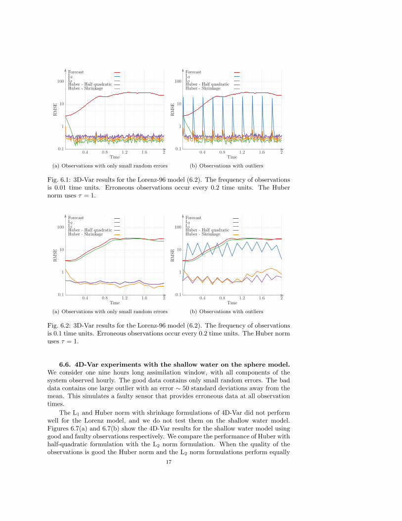
The optimization proceeds in stages of inner and outer iterations. The inner iter-ations aim to find an iterate which minimizes the cost function for a particular valueof the penalty parameter (µ). The outer iterations involves increasing the penaltyparameter and updating the Lagrange multipliers. For experimental uniformity, weuse 15 outer iterations with 3D-Var, 4D-Var, and LETKF for all formulations: L1,Huber with ADMM, and Huber with half-quadratic solutions. Figures 6.1(a) and6.3(a) show that all formulations perform very well at high observation frequency(one observation every 0.01 units) and using good data. At a low observation fre-quency with good data the L1 formulation does not perform as well as the two Huberformulations, as seen in Figures 6.2(a) and 6.4(a).

For frequent (good) observations both L1 and L2 formulations perform well, evenwhen outliers are present in the data, as seen in Figures 6.1(b) and 6.3(b). However, atlow frequency of measurements and when outliers are present the L2 formulation failsto produce good results, while the Huber formulations demonstrate their robustness,as seen in Figures 6.2(b) and 6.4(b).

6.4. 3D-Var experiments with the shallow water on the sphere model.Experiments with the shallow water model are performed for an assimilation windowof six hours, with all variables being observed hourly. The good data contains randomnoise but no outliers. The erroneous data contains one outlier, namely the heightcomponent at latitude 32 South, longitude 120 East and it has a value which is ∼ 50standard deviations away from the mean. This outlier occurs at all observation timesand hence simulates one faulty sensor periodically providing incorrect observationvalues.

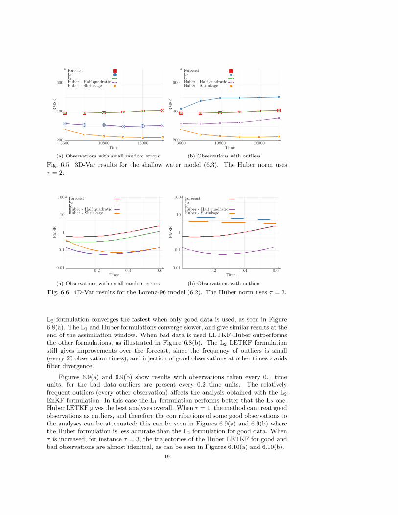
Figures 6.5(a) and 6.5(b) present the results of assimilating good and erroneousobservations ,respectively. Root mean square errors (RMSE) are shown for trajectoriescorresponding to forecast, L1, L2, and two implementations of Huber norm. TheHuber norm implementations perform as well as the L2 norm analysis when only goodobservations are used. When the observations contain outliers, the L2 norm analysisis inaccurate. However, the Huber norm analysis is robust and remains is unaffectedby the quality of observations. The L1 norm analysis also remains unaffected by thequality of observations, however, its errors are similar to those of the forecast; theL1 formulation does not use effectively the information from the good observations.Consequently, the Huber norm offers the best 3D-Var formulation, leading to analysesthat are both accurate and robust.

6.5. 4D-Var experiments with the Lorenz-96 model. 4D-Var experimentswith Lorenz model are performed for one assimilation window of 0.6 units. All com-ponents are observed every 0.1 units. The good data contains random noise but nooutliers. The erroneous data contains one outlier at all observation times and its value∼ 100 standard deviations away from the mean.

Figure 6.6(a) presents the 4D-Var results with good data. The performance ofthe Huber-4D-Var with half-quadratic formulation matches the performance of L2

formulation. The analyses provided by L1 and Huber formulations with shrinkage areless accurate. Figure 6.6(b) presents the results of assimilating data with outliers.The 4D-Var-Huber analysis using the half quadratic formulation remains unaffectedby the data errors. All other formulations (L1, L2, and Huber with shrinkage) arenegatively impacted by the presence of outliers.

16

0.1

1

10

100

0.4 0.8 1.2 1.6 2

RM

SE

Time

ForecastL2L1Huber - Half quadraticHuber - Shrinkage

(a) Observations with only small random errors

0.1

1

10

100

0.4 0.8 1.2 1.6 2

RM

SE

Time


(b) Observations with outliers

Fig. 6.1: 3D-Var results for the Lorenz-96 model (6.2). The frequency of observationsis 0.01 time units. Erroneous observations occur every 0.2 time units. The Hubernorm uses τ = 1.

0.1

1

10

100

0.4 0.8 1.2 1.6 2

RM

SE

Time



0.1

1

10

100

0.4 0.8 1.2 1.6 2

RM

SE

Time



Fig. 6.2: 3D-Var results for the Lorenz-96 model (6.2). The frequency of observationsis 0.1 time units. Erroneous observations occur every 0.2 time units. The Huber normuses τ = 1.

6.6. 4D-Var experiments with the shallow water on the sphere model.We consider one nine hours long assimilation window, with all components of thesystem observed hourly. The good data contains only small random errors. The baddata contains one large outlier with an error ∼ 50 standard deviations away from themean. This simulates a faulty sensor that provides erroneous data at all observationtimes.

The L1 and Huber norm with shrinkage formulations of 4D-Var did not performwell for the Lorenz model, and we do not test them on the shallow water model.Figures 6.7(a) and 6.7(b) show the 4D-Var results for the shallow water model usinggood and faulty observations respectively. We compare the performance of Huber withhalf-quadratic formulation with the L2 norm formulation. When the quality of theobservations is good the Huber norm and the L2 norm formulations perform equally

17

0.1

1

10

100

0.4 0.8 1.2 1.6 2

RM

SE

Time


(a) Observations with only small random errors.Observations taken every 0.01 time units.

0.1

1

10

100

0.4 0.8 1.2 1.6 2

RM

SE

Time


(b) Observations with outliers. Observationstaken every 0.01 time units.

Fig. 6.3: 3D-Var results for the Lorenz-96 model (6.2). The frequency of observationsis 0.01 time units. Erroneous observations occur every 0.2 time units. The Hubernorm uses τ = 3.

0.1

1

10

100

0.4 0.8 1.2 1.6 2

RM

SE

Time


(a) Observations with only small random errors.Observations taken every 0.1 time units.

0.1

1

10

100

0.4 0.8 1.2 1.6 2

RM

SE

Time


(b) Observations with outliers. Observationstaken every 0.1 time units.

Fig. 6.4: 3D-Var results for the Lorenz-96 model (6.2). The frequency of observationsis 0.1 time units. Erroneous observations occur every 0.2 time units. The Huber normuses τ = 3.

well. When the observations contain outliers the L2 formulation gives inaccurateanalyses, while the Huber norm formulation is robust and continues to provide goodresults.

6.7. EnSRF experiments with the Lorenz-96 model. In this section wediscuss the results of the LETKF implementations based on the L1, L2, and Hubernorms. We note that, due to localization the data outliers in LETFK will impact thestates in only small regions of the domain. The number of ensemble members for theexperiments is 20.

Assimilation experiments are carried out with different frequencies for outliersin the observations. Figures 6.8(a) and 6.8(b) show results with observations takenevery 0.01 time units; for the bad data outliers are present every 0.2 time units. The

18

200

400

600

3600 10800 18000

RM

SE

Time


(a) Observations with small random errors

200

400

600

3600 10800 18000

RM

SE

Time



Fig. 6.5: 3D-Var results for the shallow water model (6.3). The Huber norm usesτ = 2.

0.01

0.1

1

10

100

0.2 0.4 0.6

RM

SE

Time



0.01

0.1

1

10

100

0.2 0.4 0.6

RM

SE

Time



Fig. 6.6: 4D-Var results for the Lorenz-96 model (6.2). The Huber norm uses τ = 2.

L2 formulation converges the fastest when only good data is used, as seen in Figure6.8(a). The L1 and Huber formulations converge slower, and give similar results at theend of the assimilation window. When bad data is used LETKF-Huber outperformsthe other formulations, as illustrated in Figure 6.8(b). The L2 LETKF formulationstill gives improvements over the forecast, since the frequency of outliers is small(every 20 observation times), and injection of good observations at other times avoidsfilter divergence.

Figures 6.9(a) and 6.9(b) show results with observations taken every 0.1 timeunits; for the bad data outliers are present every 0.2 time units. The relativelyfrequent outliers (every other observation) affects the analysis obtained with the L2

EnKF formulation. In this case the L1 formulation performs better that the L2 one.Huber LETKF gives the best analyses overall. When τ = 1, the method can treat goodobservations as outliers, and therefore the contributions of some good observations tothe analyses can be attenuated; this can be seen in Figures 6.9(a) and 6.9(b) wherethe Huber formulation is less accurate than the L2 formulation for good data. Whenτ is increased, for instance τ = 3, the trajectories of the Huber LETKF for good andbad observations are almost identical, as can be seen in Figures 6.10(a) and 6.10(b).

19

100

300

500

0 7200 14400 21600 28800

RM

SE

Time

ForecastL2Huber - Half quadratic


100

300

500

0 7200 14400 21600 28800

RM

SE

Time

ForecastL2Huber - Half quadratic


Fig. 6.7: 4D-Var results for the shallow water model (6.3). The Huber norm usesτ = 2.

0.001

0.01

0.1

1

10

100

0.4 0.8 1.2 1.6 2

RM

SE

Time

ForecastL2L1Huber - Half quadratic


0.001

0.01

0.1

1

10

100

0.4 0.8 1.2 1.6 2

RM

SE

Time



Fig. 6.8: LETKF results for the Lorenz-96 model (6.2). The frequency of observationsis 0.01 time units. Erroneous observations occur every 0.2 time units. The Huber normuses τ = 1.

6.8. EnSRF experiments with the shallow water on the sphere model.The shallow water model (6.3) experiments use ensembles with 30 members. Theinitial ensemble perturbation is normal, with a standard deviation of 5% of the back-ground state for each component. Figure 6.12 shows the analysis errors for the L1,L2, and Huber LETKF formulations. The Huber half quadratic LETKF providesanalyses that are as accurate as the L2 formulation analyses when only good data isused. When outliers are present, however, the L2 results are very inaccurate. TheHuber formulation is almost completely unaffected by the data outliers, and providesequally better analyses with and without data outliers. The L1 formulation resultsare also unaffected by outliers, but their overall accuracy is quite low.

7. Conclusions. This papers develops a systematic framework for performingrobust 3D-Var, 4D-Var, and ensemble-based filtering data assimilation. The tradi-tional algorithms are formulated as optimizations problems where the cost functionsare L2 norms of background and observation residuals; the L2 norm choice correspondsto Gaussianity assumptions for background and observation errors, respectively. The

20

0.01

0.1

1

10

100

0.4 0.8 1.2 1.6 2

RM

SE

Time



0.01

0.1

1

10

100

0.4 0.8 1.2 1.6 2

RM

SE

Time



Fig. 6.9: LETKF results for the Lorenz-96 model (6.2). The frequency of observationsis 0.1 time units. Erroneous observations occur every 0.2 time units. The Huber normuses τ = 1.

0.001

0.01

0.1

1

10

100

0.4 0.8 1.2 1.6 2

RM

SE

Time



0.001

0.01

0.1

1

10

100

0.4 0.8 1.2 1.6 2

RM

SE

Time



Fig. 6.10: LETKF results for the Lorenz-96 model (6.2). The frequency of obser-vations is 0.01 time units. Erroneous observations occur every 0.2 time units. TheHuber norm uses τ = 3.

L2 norm formulation has to make large corrections to the optimal solution in orderto accommodate outliers in the data. Consequently, a few observations containinglarge errors can considerably deteriorate the overall quality of the analysis. In orderto avoid this effect traditional data quality control rejects certain observations, whichmay result in loss of useful information. A more recent approach performs a one-time,off-line adjustment of the data weights based on the estimated data quality.

The robust data assimilation framework described herein reformulates the under-lying optimization problems using L1 and Huber norms. The resulting robust dataassimilation algorithms do not reject any observations. Moreover, the relative impor-tance weights of the data are not decided off-line, but rather are adjusted iterativelyfor each observation based on their deviation from the mean forecast. Numerical re-sults show that the L1 norm formulation is very robust, being the least affected bypresence of outliers. However, the resulting analyses are inaccurate: the L1 norm re-jects not only outliers, but useful information as well. The Huber norm formulation is

21

0.01

0.1

1

10

100

0.4 0.8 1.2 1.6 2

RM

SE

Time



0.01

0.1

1

10

100

0.4 0.8 1.2 1.6 2

RM

SE

Time



Fig. 6.11: LETKF results for the Lorenz-96 model (6.2). The frequency of observa-tions is 0.1 time units. Erroneous observations occur every 0.2 time units. The Hubernorm uses τ = 3.

200

400

600

7200 14400 21600 28800 36000 43200

RM

SE

Time



200

400

600

7200 14400 21600 28800 36000 43200

RM

SE

Time



Fig. 6.12: LETKF results for the shallow water model (6.3). The Huber norm usesτ = 1.

able to fully use the information from “good data” while remaining robust (rejectingthe influence of outliers). We consider two solution methods for Huber norm opti-mization. The shrinkage operator solution displays slow convergence and can becomeimpractical in real-life problems. The Huber norm solution using the half-quadraticformulation seems to be the most suitable approach for large scale data assimila-tion applications. It is only slightly more expensive than the traditional L2 4D-Varapproach, and yields good results both in the absence and in the presence of dataoutliers. Future work will apply robust data assimilation algorithms using a Hubernorm formulation with a half-quadratic solution to real problems using the WeatherResearch and Forecasting model [31].

REFERENCES

[1] A. Attia, V. Rao, and A. Sandu. A hybrid Monte-Carlo sampling smoother for four dimensionaldata assimilation. Ocean Dynamics, Submitted, 2014.

[2] A. Attia, V. Rao, and A. Sandu. A sampling approach for four dimensional data assimilation.

22

In Proceedings of the Dynamic Data Driven environmental System Science Conference,2014.

[3] A. Aved, F. Darema, and E. Blasch. Dynamic data driven application systems. www.1dddas.org,2014.

[4] S. Boyd, N. Parikh, E. Chu, B. Peleato, and J. Eckstein. Distributed optimization and statisticallearning via the alternating direction method of multipliers. Foundations and Trends inMachine Learning, 3(1):1–122, 2011.

[5] D. G. Cacuci, M. Ionescu-Bujor, and I. M. Navon. Sensitivity and uncertainty analysis, VolumeII: applications to large-scale systems. CRC Press, 2005.

[6] A. Cioaca, M. Alexe, and A. Sandu. Second-order adjoints for solving PDE-constrained opti-mization problems. Optimization methods and software, 27(4-5):625–653, 2012.

[7] A Cioaca and A Sandu. An optimization framework to improve 4D-Var data assimilationsystem performance. Journal of Computational Physics, 275:377–389, 2014.

[8] R. Daley. Atmospheric data analysis, volume 2. Cambridge University Press, 1993.[9] A.M. Ebtehaj, M. Zupanski, G. Lerman, and E. Foufoula-Georgiou. Variational data assimila-

tion via sparse regularization. arXiv preprint arXiv:1306.1592, 2013.[10] T. Eltoft, T. Kin, and T.-W. Lee. On the multivariate Laplace distribution. IEEE Signal

Procesing Letters, 13(5):300–303, 2006.[11] A. Guitton and W.M. Symes. Robust inversion of seismic data using the huber norm.

Geophysics, 68(4):1310–1319, 2003.[12] A. Hollingsworth, D.B. Shaw, P. Lonnberg, L. Illari, K. Arpe, and A.J. Simmons. Monitoring of

observation and analysis quality by a data assimilation system. Monthly Weather Review,114(5):861–879, 1986.

[13] B.R. Hunt, E.J. Kostelich, and I. Szunyogh. Efficient data assimilation for spatiotemporalchaos: A local ensemble transform Kalman filter. Physica D, 230:112–126, 2007.

[14] E. Kalnay. Atmospheric modeling, data assimilation, and predictability. Cambridge UniversityPress, 2003.

[15] A.C. Lorenc. Analysis methods for numerical weather prediction. Royal Meteorological Society,Quarterly Journal, 112:1177–1194, 1986.

[16] A.C. Lorenc. A Bayesian approach to observation quality control in variational and statisticalassimilation. Defense Technical Information Center, 1993.

[17] A.C Lorenc and O. Hammon. Objective quality control of observations using bayesian methods.theory, and a practical implementation. Quarterly Journal of the Royal MeteorologicalSociety, 114(480):515–543, 1988.

[18] E. N. Lorenz. Predictabilty: A problem partly solved. In Proceedings of Seminar onPredictability, pages 40–58, 1996.

[19] I. M. Navon and R. De Villiers. The application of the Turkel-Zwas explicit large time-stepscheme to a hemispheric barotropic model with constraint restoration. Monthly weatherreview, 115(5):1036–1052, 1987.

[20] I. M. Navon and J. Yu. Exshall: A Turkel-Zwas explicit large time-step FORTRAN program forsolving the shallow-water equations in spherical coordinates. Computers and Geosciences,17(9):1311 – 1343, 1991.

[21] M. Nikolova and M.K. Ng. Analysis of half-quadratic minimization methods for signal andimage recovery. SIAM Journal on Scientific computing, 27(3):937–966, 2005.

[22] V. Rao and A. Sandu. A posteriori error estimates for DDDAS inference problems. ProcediaComputer Science, 29:1256–1265, 2014.

[23] V. Rao and A. Sandu. A posteriori error estimates for the solution of variational inverseproblems. SIAM/ASA Journal on Uncertainty Quantification, 2015.

[24] S. Roh, M.G. Genton, M. Jun, I. Szunyogh, and I. Hoteit. Observation quality control with arobust ensemble Kalman filter. Monthly Weather Review, 141(12):4414–4428, 2013.

[25] E. D. N. Ruiz and A. Sandu. A derivative-free trust region framework for variational dataassimilation. Journal of Computational and Applied Mathematics, 2015.

[26] A. Sandu and T. Chai. Chemical data assimilation—An overview. Atmosphere, 2(3):426–463,2011.

[27] A. Sandu, D. N. Daescu, G. R. Carmichael, and T. Chai. Adjoint sensitivity analysis of regionalair quality models. Journal of Computational Physics, 204(1):222–252, 2005.

[28] A. Sandu and L. Zhang. Discrete second order adjoints in atmospheric chemical transportmodeling. Journal of Computational Physics, 227(12):5949–5983, 2008.

[29] A. St-Cyr, C. Jablonowski, J.M. Dennis, H.M. Tufo, and S.J. Thomas. A comparison oftwo shallow water models with nonconforming adaptive grids. Monthly Weather Review,136:1898–1922, 2008.

[30] C. Tavolato and L. Isaksen. On the use of a Huber norm for observation quality control in the

23

www.1dddas.org

ECMWF 4D-Var. Quarterly Journal of the Royal Meteorological Society, 2014.[31] WRF. The weather research forecasting model. http://wrf-model.org.

Appendix A. Multivariate Laplace distribution of observation errors.The univariate Laplace distribution models an exponential decay on both sides

away from the mean µ; the probability density function is:

P(z) = (2λ)−1 exp (− |z − µ| /λ) , E [z] = 0, Var [z] = 2λ2.

Let z be the scaled innovation vector (3.1), with E [z] = 0, and Cov [z] = I. Assumethat each component error has a univariate Laplace distribution, and that the com-ponent errors are independent. The observation part of the variational cost function(3.3) is the log-likelihood:

− log P(z) ∝ λ−1n∑`=1

|z`| , E [z] = µ, Cov [z] = 2λ2 I.

Our formulation of the variational cost function (3.3) uses λ = 2, which translates inan assumed variance for each component of 8.

The multivariate Laplace distribution is [10]

P(z) =2

(2λ)(n+2)/4 πn/2

K(n−2)/2

(2λ ‖z− µ‖

2R−1

)‖z− µ‖(n−2)/2R−1

,(A.1)

where Kn is the modified Bessel function of the second kind and order n. From (A.1)we have that

E [z] = µ, Cov [z] = λR.

For large deviations ‖z− µ‖R−1 →∞ the pdf (A.1) is approximated by

(A.2) P(z) ≈ ‖z− µ‖(1−n)/2R−1 exp

(− 2

λ‖z− µ‖R−1

).

Let z be the scaled innovation vector (3.1), with E [z] = 0, and Cov [z] = I. Theobservation part of the variational cost function (3.3) is the log-likelihood, which forlarge deviations is approximately equal to:

(A.3) log P(z) ≈ n− 1

2log ‖z‖2 +

2

λ‖z‖2 .

24

Documents

Computational Science Laboratory Technical Report CSL-TR