TAMPERE UNIVERSITY OF TECHNOLOGYDepartment of Information Technology

Jarno Seppänen

COMPUTATIONAL MODELS OF MUSICAL METERRECOGNITION

Master of Science Thesis

Subject approved by the department council on August 22nd, 2001.Supervisors: Professor Petri Haavisto

M.Sc. Anssi KlapuriM.Sc. Matti Hämäläinen

Preface

This work was carried out at the Speech and Audio Systems Laboratory at Nokia ResearchCenter as a continuation to initial research at the Audio Research Group at Tampere Uni-versity of Technology. I am equally grateful to my colleagues at the Audio Research Groupand at the Speech and Audio Systems Laboratory. I would especially like to thank Jari Yli-Hietanen and Anssi Klapuri for professional and curricular guidance and encouragementand Matti Hämäläinen and Petri Haavisto for endorsement and positive feedback.

I am thankful for the Audio Research Group for providing assistance in the manual anno-tation of music; without their help, this work would not have been possible. Thanks to EricScheirer for sharing his beat tracker implementation and to Igor Cadez for sharing the EMalgorithm implementation with the research community. Thanks to Juha Laine for supply-ing the LATEX template to work with. I would also like to mention that all trademarks thatpossibly appear in this thesis are acknowledged.

My warmest thanks go to my parents Mirja and Jouko Seppänen and to my sister Katri.Finally, I wish to thank Tuire for her wholehearted love and support.

Tampere, November 1st, 2001

Jarno Seppänen

ii

Table of Contents

Preface . . . . . . . . . . . . . . . . . . . . . . . . . . . . . . . . . . . . ii

Table of Contents . . . . . . . . . . . . . . . . . . . . . . . . . . . . . . iii

Abstract . . . . . . . . . . . . . . . . . . . . . . . . . . . . . . . . . . . . v

Tiivistelmä . . . . . . . . . . . . . . . . . . . . . . . . . . . . . . . . . . vi

Glossary . . . . . . . . . . . . . . . . . . . . . . . . . . . . . . . . . . . vii

1 Introduction . . . . . . . . . . . . . . . . . . . . . . . . . . . . . . . . . 1

2 Theoretical background . . . . . . . . . . . . . . . . . . . . . . . . . . . 42.1 Rhythm . . . . . . . . . . . . . . . . . . . . . . . . . . . . . . . . . 42.2 Music notation . . . . . . . . . . . . . . . . . . . . . . . . . . . . . 52.3 Meter and the metrical structure . . . . . . . . . . . . . . . . . . . . 6

2.3.1 Hierarchy of meter . . . . . . . . . . . . . . . . . . . . . . . 72.3.2 Accents . . . . . . . . . . . . . . . . . . . . . . . . . . . . . 10

2.4 Statistical pattern recognition . . . . . . . . . . . . . . . . . . . . . 112.4.1 Linear discriminant analysis . . . . . . . . . . . . . . . . . . 132.4.2 Multivariate Gaussian modeling . . . . . . . . . . . . . . . . 142.4.3 Gaussian mixture modeling . . . . . . . . . . . . . . . . . . 142.4.4 Feature selection . . . . . . . . . . . . . . . . . . . . . . . . 15

3 Previous models . . . . . . . . . . . . . . . . . . . . . . . . . . . . . . . 173.1 Rule-based search models . . . . . . . . . . . . . . . . . . . . . . . 183.2 Multiple-agent models . . . . . . . . . . . . . . . . . . . . . . . . . 203.3 Multiple-oscillator models . . . . . . . . . . . . . . . . . . . . . . . 213.4 Procedural models . . . . . . . . . . . . . . . . . . . . . . . . . . . 223.5 Probabilistic models . . . . . . . . . . . . . . . . . . . . . . . . . . 233.6 Commercial systems . . . . . . . . . . . . . . . . . . . . . . . . . . 24

4 Proposed model . . . . . . . . . . . . . . . . . . . . . . . . . . . . . . . 254.1 Sound onset detection . . . . . . . . . . . . . . . . . . . . . . . . . 26

4.1.1 Filterbank analysis . . . . . . . . . . . . . . . . . . . . . . . 284.1.2 Channel amplitude envelope . . . . . . . . . . . . . . . . . . 294.1.3 Amplitude envelope thresholding . . . . . . . . . . . . . . . 304.1.4 Rough sound duration estimation . . . . . . . . . . . . . . . 314.1.5 Combining bandwise raw onsets . . . . . . . . . . . . . . . . 32

4.2 Tatum grid estimation . . . . . . . . . . . . . . . . . . . . . . . . . 324.2.1 Inter-onset interval computation . . . . . . . . . . . . . . . . 324.2.2 Greatest common divisor approximation . . . . . . . . . . . . 334.2.3 Inter-onset interval histogram . . . . . . . . . . . . . . . . . 334.2.4 Remainder error thresholding . . . . . . . . . . . . . . . . . 34

iii

4.2.5 Tatum phase estimation . . . . . . . . . . . . . . . . . . . . . 344.2.6 Metrical ground estimation . . . . . . . . . . . . . . . . . . . 35

4.3 Phenomenal accent estimation . . . . . . . . . . . . . . . . . . . . . 364.3.1 Music corpus processing . . . . . . . . . . . . . . . . . . . . 364.3.2 Acoustic feature extraction . . . . . . . . . . . . . . . . . . . 384.3.3 Accent recognition . . . . . . . . . . . . . . . . . . . . . . . 404.3.4 Phenomenal accent model . . . . . . . . . . . . . . . . . . . 44

4.4 Beat grid estimation . . . . . . . . . . . . . . . . . . . . . . . . . . 454.4.1 Beat interpretation likelihood . . . . . . . . . . . . . . . . . 464.4.2 Beat period prior probability . . . . . . . . . . . . . . . . . . 464.4.3 Causal beat grid assignment . . . . . . . . . . . . . . . . . . 47

4.5 Estimation of subordinate metrical levels . . . . . . . . . . . . . . . 48

5 Model performance . . . . . . . . . . . . . . . . . . . . . . . . . . . . . 495.1 Performance measure . . . . . . . . . . . . . . . . . . . . . . . . . . 495.2 Results . . . . . . . . . . . . . . . . . . . . . . . . . . . . . . . . . 50

6 Conclusions . . . . . . . . . . . . . . . . . . . . . . . . . . . . . . . . . . 53

References . . . . . . . . . . . . . . . . . . . . . . . . . . . . . . . . . . 56

A Music corpus . . . . . . . . . . . . . . . . . . . . . . . . . . . . . . . . . 62

B Acoustic signal features . . . . . . . . . . . . . . . . . . . . . . . . . . . 68

iv

Abstract

TAMPERE UNIVERSITY OF TECHNOLOGYDepartment of information technologySignal processing laboratorySEPPÄNEN, JARNO: Computational models of musical meter recognitionMaster of Science thesis, 61 pages, 11 enclosure pagesExaminers: Prof. Petri Haavisto, M.Sc. Anssi Klapuri, and M.Sc. Matti HämäläinenFunding: Nokia OyjNovember 2001Keywords: music analysis, rhythm, meter, beat, tatum, phenomenal accent

The thesis proposes an algorithm for the recognition of musical meter from acoustic signalsof music. Musical meter is a part of rhythm that is constantly present in music, as it spansthe musical time base. The proposed model is capable of finding metrical levels, includingthe beat and the tatum, in real time from a musical audio signal. The model comprises fourmain components: an onset detector, a tatum estimator, a phenomenal accent model, anda beat estimator. The onset detector finds distinct sound onsets from an acoustic signal,using multiband signal processing. After this, the tatum, which is the lowest metrical level,is computed from onset times. Phenomenal accents are computed from a set of 16 acousticsignal features using Bayesian pattern recognition. The tatum and the accents then yieldthe beat. The proposed model operates causally and is able to respond to tempo changes.The design of the model aims at generality in regard to musical genres, and thus the modelis trained and tested using 330 music excerpts from multiple genres. The model perfor-mance varies according to the rhythmic difficulty of the input signal. Most pop/rock musicposes no problems for the algorithm, while classical music and expressive jazz pieces areintractable. The model produces more errors than Eric Scheirer’s beat tracker, but at thesame time it follows more metrical levels than Scheirer’s model. The results of this the-sis are directly applicable in music production and post-processing. The access to musicaltime enables new levels of productivity and automation in both music software and hard-ware. Meter-synchronized comparison, mixing, and editing of pieces of music is possible.Robust meter recognition is a vital component of music information retrieval applications.

v

Tiivistelmä

TAMPEREEN TEKNILLINEN KORKEAKOULUTietotekniikan osastoSignaalinkäsittelyn laitosSEPPÄNEN, JARNO: Musiikin metrin tunnistuksen laskennallisia mallejaDiplomityö, 61 sivua, 11 liitesivuaTarkastajat: prof. Petri Haavisto, DI Anssi Klapuri ja DI Matti HämäläinenRahoittaja: Nokia OyjMarraskuu 2001Avainsanat: musiikkianalyysi, rytmi, metri, isku, tatum, fenomenaalinen aksentti

Tässä työssä kuvataan menetelmä musiikin metrin tunnistamiseksi akustisesta musiikkisig-naalista. Musiikin metri on rytmin osa, joka virittää musikaalisen aikajanan ja on siksi kokoajan läsnä musiikissa. Tässä esitetty menetelmä etsii iskun ja tatumin sekä muita metrisiätasoja musiikkisignaalista reaaliajassa. Malli jakautuu neljään pääosaan, jotka ovat aluke-tunnistin, tatumin havaitsija, fenomenaalisen aksentin malli sekä iskun havaitsija. Aluke-tunnistin etsii musiikkisignaalista erillisten äänten alkuhetkiä taajuuskaistoihin perustuvansignaalinkäsittelyn avulla. Äänten alkuhetkien perusteella lasketaan metrin alin taso eli ta-tum. Fenomenaalinen aksentti lasketaan 16:sta akustisesta signaalipiirteestä soveltamallabayesiläistä hahmontunnistusta. Kuvattu menetelmä toimii kausaalisesti ja pystyy reagoi-maan myös tempon vaihteluihin. Työssä esitelty menetelmä optimoidaan ja testataan käyt-tämällä 330:tä CD-levyltä otettua musiikkinäytettä. Näytteet sisältävät useita musiikkityy-lejä, koska menetelmä on suunniteltu musiikkityylistä riippumattomaksi. Menetelmän suo-rituskyky vaihtelee musiikin rytmin vaikeuden mukaan. Suurin osa pop- ja rockmusiikistaei aiheuta ongelmia menetelmälle, mutta klassisesta musiikista ja monimutkaisesta jazzistase ei suoriudu. Malli antaa enemmän virheitä kuin Eric Scheirerin kehittämä iskunseuraaja-algoritmi, mutta toisaalta se antaa myös tuloksia useammasta metrin tasosta kuin Scheirerinmalli. Tämän työn tuloksia voidaan suoraan soveltaa musiikin tuotannossa ja jälkikäsitte-lyssä. Musikaalisen ajan käsittely antaa uusia mahdollisuuksia tehostaa ja automatisoidamusiikkiohjelmistoja ja -laitteita sekä niiden käyttöä. Musiikkikappaleiden vertailu, mik-saus ja muokkaus on mahdollista tahdistaa metrin avulla. Vakaasti toimiva metrin tunnistuson tärkeä osa musiikin hakusovelluksia.

vi

Glossary

A posteriori The posterior probability distribution p(ω|x) of an event ω in Bayesianpattern recognition.

A priori The prior probability P (ω) of an event ω in Bayesian pattern recognition.Accelerando Italian for a gradual acceleration of tempo.Accent Musical stress applied to a note.Asynchronous Data transfer that happens irregularly, not controlled by a clock; also

called event- or message-based transfer; the transfer mode used withsymbolic data.

Bar See measure.Beat The most salient pulsation, both an individual pulse and all the pulses

on the same level; equals foot tapping times; some other literature uses“tactus” to refer to beats and “beat” to refer to pulses.

Beat grid The set of time instants that belong to the beat level.Beat period The time between neighboring pulses on the beat level; in other literature

also referred to as inter-beat interval, or IBI.BPF A band-pass filter.BPM Beats per minute; unit of tempo, or beat rate; in other literature also re-

ferred to as M.M., or Mälzel’s metronome, in honor of Johannes Mälzel,the inventor of the metronome.

Cepstrum A standard speech and audio processing representation for spectralshape.

DCT The discrete cosine transform, a signal processing mechanism used incepstrum computation.

EM The expectation-maximization algorithm is used to optimize the para-meters of a Gaussian mixture model (GMM).

FFT The fast Fourier transform; usually used to denote the discrete Fouriertransform.

GCD Greatest common divisor; an integer factor of a set of integers.GMM Gaussian mixture model; Bayesian pattern recognition with a specific

class of likelihood functions.Grid A set of regularly spaced time instants.Grouping The combination of notes together into groups that contain one musical

motive.IIR A class of digital filters that exhibit an infinite impulse response.IOI Inter-onset interval; the time between two sound onsets.Isochronous Occurring at equal intervals of time.LDA Linear discriminant analysis, a minimum-distance pattern recognition

method.

vii

Likelihood A probability distribution function (PDF) p(x|ω) for representing evi-dence in Bayesian pattern recognition.

LPF A low-pass filter.MAP Maximum a posteriori; a Bayesian pattern recognition method assuming

differing prior probabilities.Measure A metrical unit subsuming several beats; also called the bar.Meter The hierarchy of pulsations that is always present when listening to mu-

sic; comprises measure, beat, and tatum, among other levels.Metrical grid A transcription of meter that shows all the (relevant) metrical levels.MIDI A data format for storing and transmitting music in a symbolic format;

shorthand for Musical Instrument Digital Interface.ML Maximum likelihood; a Bayesian pattern recognition method assuming

equal prior probabilities.Note A singular musical event.Offbeat A time instant that does not coincide with a beat.Onset The starting point (attack) of an individual note.PDF The probability distribution function of a random variable, denoted p(x).Pulse An individual time instant; also a set of pulses with a common period; in

other literature also referred to as “beat.”Ritardando Italian for a gradual deceleration of tempo.RMS Root–mean–square; a technical measure of signal level.Rubato Italian for flexible variation of tempo; also tempo rubato.Sforzando Italian for sudden and strong accent; plural sforzandi.Signal A discrete-time function, where time takes values from a regular clock;

signals are transfered synchronously.Symbol A function which changes its values irregularly; symbolic transfers are

asynchronous.Synchronous Data transfer that happens according to a regular clock; the transfer mode

of signals.Tatum The lowest/smallest metrical unit; the pulse that has the fastest pulsation.

In some literature referred to as clock.Tatum grid The set of time instants, i.e. pulses, on the tatum metrical level.Tempo Italian for the time (i.e. speed) of music; expressed as the beat rate, often

measured in BPM units; plural tempi.Time signature The numeric indication of musical measure length in the beginning of

scores.

viii

1 Introduction

Music is as universal a phenomenon as speech: people all over the world play and enjoymusic. Music exists in different forms in different cultures, but still the basic value of musicis independent of cultural aspects. Music is understood as thought-provoking art or a usefultool, it evokes feelings and discussion, and is used for relaxation everywhere. Music hasexisted probably as long as, or even longer than speech. It seems that both speech and musichave fulfilled important requirements in the history of mankind, in rational and emotionalcommunication, respectively. [CK99]

In this thesis I discuss musical rhythm, which is as profound and historical a phenomenonas music itself. Musical styles have changed over time, from baroque to post-modern, andfrom acoustic to electronic, but rhythm has sustained its importance within the aesthetics ofmusic.

Humans possess a natural ability to absorb and appreciate music, even if they are completelyunaware of the theory of music. Although intricate theories of the composition of musicexist, music is always listened to with emotions. I argue that the natural music-listeningability best manifests itself in the act of dancing. In fact, rhythm as a whole is speculatedto being a direct consequence of movement [Cla99, p. 495]. Dancing is a concretizationof music appreciation, through swinging of hands and clattering of feet. The speed andtiming of dancing is purely based on the rhythm of music, and the principal features humansrecognize from rhythm are indeed connected with dancing [EGP00].

The need to automatically process music was justified when the phonograph was invented.Here, ‘automatic processing’ is used to refer to applications such as the automatic retrievaland playback of music from a record collection. Recorded music has been available al-ready in the 19th century, and the amount of recorded music has since increased fast, butthe automatic analysis and processing of music has become feasible only since the 1980’safter computer technology had advanced to a sufficient level. Manual post-processing ofrecorded music has been carried out since musique concrète on the 1940’s [Pal99], andit even became a widely accepted means to create new music through the invention ofsampling. However, only a limited number of automatic or semiautomatic music post-processing tools exist currently, and many of them still are quite far from really functionalautomated processing of recorded music.

Automatic processing of music can refer to automatically recognizing, retrieving, editing,and playing recorded music, based on very simple commands or even no commands at allfrom a user. The scope of this work is in processing recorded music, that is, music inthe form of acoustic signals. The processing of acoustic signals of music poses a signif-icant change of field and an increase in level of difficulty compared to the processing ofscores of music. During the last ten years, the theory and practice of signal processing ap-

1

plied to acoustic musical signals, termed musical signal processing, has advanced rapidly.Wherever possible, digital signal processing has replaced earlier acoustic or analog elec-trical means in the production and consumption of music. Signal processing has enabledperceptual compression of music, based on investigations of auditory perception. There isalso a body of recent research on music perception, of which the part on rhythm and meterestimation, beat and tempo tracking, and sound onset detection are relevant to this thesis.

An important component in the automated processing of music is the analysis, i.e., un-derstanding of musical signals by a computer, and this is also the component still missingas of today. In analyzing musical signals, the aim is to understand and replicate the wayhumans experience music, and thus the research into computational analysis of musicalsignals is a combination of music psychology and signal processing. Once we have a com-putational model of music perception, the number of applications appear limitless. Massivearchives of music become highly useful and usable even for non-experts. The maintenanceand assembly of coherent musical databases becomes quite straightforward. A collectionof music will transform into a unique new musical instrument, played through the musicperception model capable of fusing songs and sounds from the collection. One prospect ofmusic perception model is the categorization of music. With the aid of perceptual models,computers will be able to classify musical recordings to slow or fast, to classical or modern,to instrumental or vocal, and according to genre. This will be very useful in all the numer-ous situations where music is used: for listeners, radio stations, libraries, music and filmproducers, musicians, etc.

The concept of rhythm breaks down into two constituent parts: grouping and meter [LJ83].I am mainly interested in the latter phenomenon, into which e.g. the percept of beat be-longs. In this thesis, I propose a novel method for musical meter recognition at the beatand tatum levels, where the former refers to the most salient level of meter and the latter tothe lowest metrical level. The metrical structure of a piece of music describes the compre-hension of musical time in the piece, following tempo changes such as accelerandos andritardandos [Cla99]. Recognition of musical meter is a vital subtask in approaching musicperception models.

The beat and meter recognition model proposed in this thesis is primarily a bottom-up pro-cedure. Musical knowledge is incorporated into the estimation of phenomenal accentuationof different locations in the input signal via supervised learning, but otherwise the algorithmis a stack of procedures rooted on the actual acoustic signal, with the highest-residing pro-cedure outputting the beat. The processing phases from input to output are sound onsetdetection, tatum estimation, phenomenal accent modeling, and beat estimation.

A number of previously published models on beat and meter recognition are reviewed inaddition to the proposed model. The published models vary from MIDI (Musical Instru-ment Digital Interface) analysis algorithms to audio signal processing methods, and fromsimple autocorrelation models to complex symbolic artificial intelligence systems for me-

2

ter recognition. The performance of the proposed model is compared to the performance ofone of the reviewed models [Sch98b]. The performance of the models in tracking the beatfrom commercial music excerpts is compared. The comparison was done using excerpts of330 different songs sampled from commercially published CD records.

This thesis is divided into the following chapters:

• Chapter 2, Theoretical background, introduces the reader with the theoretical conceptsused in this thesis;• Chapter 3, Previous models, reviews the previous literature related to models of meter

recognition;• Chapter 4, Proposed model, describes the construction and functionality of the pro-

posed meter recognition model;• Chapter 5, Model performance, evaluates model performance and introduces the related

constraints and measures;• Chapter 6, Conclusions, recapitulates the propositions and contributions made in this

thesis;• Appendix A, Music corpus, describes the music samples used in this research; and• Appendix B, Acoustic signal features, explains the signal description methods used in

this research.

3

2 Theoretical background

This work is based on theory of music and pattern recognition, in addition to the theory ofsignal processing. Assuming familiarity with the basics of linear signal processing, I pro-ceed to describe the parts of music theory and pattern recognition theory applied in thiswork.

2.1 Rhythm

Generally, music is composed of melody, harmony, and rhythm, and all musical worksare perceived and analyzed based on these. Rhythm and harmony are regarded as beingcomplementary to each other, in the sense that the same piece of music can be analyzedpurely from a rhythmic or a harmonic aspect, if necessary. [CK99]

Nevertheless, rhythm is a vague and ambiguous idiom, and it is hard to describe rigorously.Especially, the relationship between rhythm and meter may be hard to understand at first —this is nicely illustrated by the following quotes, in which the descriptions form a viciouscircle.

“rhythm noun 1 periodical accent and duration of notes in music. 2 type of struc-ture formed by this. . . . (see also metre, . . . )”“metre noun (US meter) . . . 3 basic rhythm of music.”Oxford Dictionary and Thesaurus, Oxford University Press, 1996

As correctly explained in the above quote, rhythms are formed from notes primarily throughthe accents and durations of notes. The accents, and thus the rhythms, are periodic in nature,which means that the note and accent patterns, or parts thereof, are not isolated but repeatagain and again over time. Looking in more detail, rhythm is caused by

• note timings and durations, in relation to neighboring notes, and• note accents, comprising e.g. sound loudness, pitch, and timbre.

These physical phenomena evoke a perceptual response to rhythm, which involves suchaspects as

• pulsation, due to the repetition of note patterns,• structure, which defines the importance of notes,• velocity, or a sensation of a relaxed vs. a hurried feeling, and• human motor abilities, which set absolute limits for rhythmic percepts. [Cla99]

4

The above properties, as well as the whole concept of rhythm, can be divided into two per-ceptual categories: grouping and meter. Like rhythm and harmony, these two categoriesalso complement each other — they can both be observed separately but a complete anal-ysis of a rhythm requires both. Meter is a description of the perceptual pulsation that isinduced by rhythms. When we listen to music, we recognize several pulsations at the sametime; therefore, meter also has multiple coexisting levels. The pulsations continue from thebeginning of music to the end. In other words, meter is present in music all the time. Group-ing, on the other hand, is a local phenomenon, and only corresponds to a limited numberof notes at a time. In grouping, sequences of notes are sectioned into separate motives bycombining notes together or separating them. [LJ83, p. 12]

Undoubtedly the single most important rhythmic property is the beat, sometimes referred toas the “tactus” [LJ83]. The beat is a part of meter, defined by the tapping of a foot by mostpeople during listening to music; beats are the points in time when people tap their foot tothe floor.1 In addition to foot-tapping, the sensation of the beat is embodied in dancing andother music-inspired acts. From this connection between the beat and human movementemerges also a preferred beat period of approximately 600–700 ms, corresponding to atempo, or beat rate, of 86–100 beats per minute (BPM) [Par94]. In engineering terms, thepreferred tempi can be interpreted as a resonance in the human response to music.

2.2 Music notation

Music on a sheet of paper is considerably different from heard music. Scheirer points outthat notation is virtually useless for music perception research due to (a) the limitationsof the music notation system, (b) the underlying assumptions, and (c) the favor for ex-pressive performance. The essence of notation is to provide instructions for playing, i.e.,generating music, not perceiving it, and this makes using notes to aid in perceiving musicill-adviced [Sch00].

Figure 2.1 shows two examples of music notation. The two examples consist of only re-peating eight notes (also called quavers) and notated accents. Accents are marked with the‘>’ symbol; whenever there is an accent symbol below or above a note, the note is playedstressed. The value 4/4 in the beginning of the example scores is the time signature, and itdetermines the duration of one measure. One can also say that the piece is “in 4/4 meter.”In this case, this means that one measure consists of four quarter notes (also called crotch-ets). In Figure 2.1 you can see how the measure boundaries are indicated with vertical lineseight quavers apart. The measure is sometimes called the bar.

1That is not to say that beats do not exist when someone does not tap at all during listening; of course the

people have to agree to tap while listening.

5

(a) M 44

� = 100B

� � �B

� � �B

� � �B

� � �B

� � �B

� � �B

� � �B

� � �

(b) M 44

B

� � �B

� � � �B

� � �B

� � �B

� �B

� � �B

� � �B

� �

Figure 2.1: Two simple isochronous trains of notes with different accent (‘>’) and similar beat (‘B’) patterns.Tempo is specified as 100 quarter notes per minute.

A particular problem with notation is the relation of the perceived beat with the notes. Onecan often hear claims that the quarter note equals the beat in notation, but this statementis generally false despite the fact that it may happen that the quarter note coincides withthe beat. Due to the essence of notation as a generative medium, it is really not possibleto assign a certain note duration to the beat from beforehand. This example illustrates thedifference of notation and music perception: even for such a profound perceptual musicconcept as the beat there is no well-defined notational counterpart. The beats are labeled inFigure 2.1 with the character ‘B,’ but this is not standard notation. The labeling is correctonly if the notated tempo and accent structure are strictly obeyed during playing.

The notations in this thesis should be used as a guide to producing small rhythmic themesand then to comparing the annotations with the perception of the generated rhythms. Inplaying the notes, I intend no extra-notational expression to be made. The beat of theexample notations has been anchored with respect to the notes by using explicit tempomarkings.

2.3 Meter and the metrical structure

Meter is the organization of music into pulses. A pulse is a set of regularly repeating timeinstants — I will also use “pulse” to refer to the individual time instants if the meaning isclear in the context. Meter is one component of rhythm, the other one being grouping. Thepulsations induced by meter are present at all times in a musical piece. The most salientpulsation is the beat, as mentioned above, and tapping along to the beat is a fundamentalmusical skill. Meter and the associated pulsations create a musical time base, making notedurations and musical measures possible. Meter contains several coexisting levels, whichare organized into a hierarchy.

Assuming a constant tempo, all metrical pulses are isochronous, i.e., the time between thepulses is constant. Meter can be measured on different levels, and the rate of pulses on lowermetrical levels is faster than on higher levels. As mentioned above, the most important and

6

interesting metrical pulsation is the beat, which resides in the vicinity of a moderate pulserate of 86–100 BPM.

However, tempo changes do complicate things somewhat. It does generally not apply thatthe absolute time between pulses does not change. On the countrary, means such as ac-celerando, ritardando and tempo rubato2 are about specifically modulating the tempo ei-ther gradually or abruptly in order to arrive at artistic ends. Under such modulation, themetrical pulses are no more isochronous, and the best general definition can only state thatthe metrical pulses be regular in time.

Observing the beat period through accelerandi and other such modulations gives a tempocurve, which depicts the tempo as a function of time since the start of the piece. It can bedebated whether structuring music with the aid of a tempo curve is useful at all or whetherit is even harmful [DH93], but tempo curves can give an intuitive starting point for pieceanalysis and even post-processing [MZ94].

2.3.1 Hierarchy of meter

There exists several levels of meter, indicating that meter is hierarchical in nature. In ad-dition to the beat, the measure, also known as the bar, and the tatum are metrical units.The measure is usually 3–4 times longer than the beat, whereas the tatum3 is (almost) al-ways shorter than the beat. The period of the measure is indicated in the time signature.The tatum is the lowest metrical level, which Bilmes describes by saying “often, it is de-fined by the smallest time interval between successive notes in a rhythmic phrase” [Bil93b,p. 22]. The tatum may equal the beat in rare cases where the shortest notes equal the beatperiod. In addition to the abovementioned levels, there are several unnamed levels of meterlocated between the tatum and the beat, between the beat and the measure and also abovethe measure.

According to Lerdahl and Jackendoff, the metrical hierarchy is built from two proper-ties [LJ83]:

1. Every pulse on a given metrical level is also a pulse on all the lower metrical levels.Moreover, pulses on a given level are strong pulses on the next-lower level, while allother pulses on that level are weak.

2. Metrical levels obey a binary/ternary division. The periods of pulses between neigh-boring metrical levels are related either by a factor of two or three.

2Meaning acceleration, deceleration, and expressive tempo changes, respectively.3The term “tatum” has been derived from “temporal atom” by Bilmes [Bil93b]. The tatum has also been

called the clock in some occasions in previous literature.

7

Figure 2.2: An example metrical grid showing hierarchy, strong/weak dichotomy, binary/ternary division, anda warped absolute time axis.

Actually, there are a few exceptions to the second rule, which are namely contemporarysongs with an odd meter, such as the exemplary Take Five by Dave Brubeck (in 5/4 meter).

After the beat, the second important metrical level is perhaps the tatum or the measure. Forcomputational music processing applications the tatum approaches the importance of thebeat. This is because the pulse intervals on all other metrical levels, including the beat, areintegral multiples of the tatum. The tatum is an ideal short-time segmentation for musicalsignals, essentially due to the fact that it is “that time division that most highly coincideswith all note onsets” [Bil93b, p. 22].

Figure 2.2 shows the transcription of metrical structure called the metrical grid togetherwith an absolute time axis. In a metrical grid, the pulses are drawn as dots, and individualmetrical levels are organized as horizontal pulse trains, with time advancing from left toright. The different levels are stacked on top of each other, with low metrical levels onbottom and high on top.4 In the example, between the tatum and the beat there is onesubordinate level. This level is a binary sublevel of the beat, and the tatum is a ternarysublevel of the subordinate level. All other divisions are binary. The large-scale levels ingeneral refer to all levels above the measure level.

Figures 2.3 and 2.4 give two examples of percussion rhythms and the associated metricalgrids. The metrical grid is transcribed on the staff labeled “Meter.” In the figures, the

4The representation of Lerdahl’s and Jackendoff’s is vertically reversed in comparison to this, i.e., they

draw the lowest metrical level on top [LJ83].

8

Meter

Bass

Snare

Hi-hat

M

M

M

44

44

44

�

�

�

�

� �

�

�

� >

> �

� = 120

� � � �

�

�

�

� �

�

�

� >

> �

� � � �

�

�

�

�

� �

�

�

� >

> �

� � � �

�

�

�

� �

�

�

� >

> �

� � � �

Figure 2.3: An example of a metrical structure, transcribed on four levels of hierarchy.

Meter

Bass

Snare

Hi-hat

M

M

M

44

44

44

�

�

�

�

�

� �

�

>

� = 120

3� �

�

�

� �

3

� �

�

�

�

� �

?

�

3

� �

�

�

� �

3

� �

3

� �

�

�

�

�

� � �

�

� �

?

�������3

? )�

>

3

� �3

� �

�

�

�

� � �

�

� �

>

�

3

� �3

� �

Figure 2.4: Another example of a metrical structure, shown on five levels of hierarchy.

tatum is the lowest horizontal pulse train on the metrical grid. In these two examples, therelationships between the beat and the tatum are clearly different. In Figure 2.3 the beat isthe second pulse train from the bottom and one beat equals two tatums, while in Figure 2.4the beat is the third-lowest level and one beat is six tatums. These examples try to illustratethat it is not possible to compute the tatum directly from the beat nor vice versa.

What is not transcribed in the example figures are the metrical levels above the measure.The metrical levels higher than the beat are collectively called the large-scale metrical struc-ture. As higher and higher levels are considered, locating the pulses becomes more andmore ambiguous even when given access to the complete score to a piece [LJ83]. Conse-quently, the analysis of large-scale metrical structure apart from the measure is not feasible.

9

2.3.2 Accents

An accent is musical stress applied to a note. The different accents on notes and voicescontribute to the sensation of the beat. On a simple isochronous train of notes, the accentu-ated notes tend to coincide with the perception of the beats. In the case where the accentsare regularly spaced and are at a moderate rate, this is obvious, while in the case where theaccents carry a rhythmic pattern, it may be harder to see.

Figure 2.1 showed two note trains with a regular and an irregular accent structure. In Fig-ure 2.1(a) the accents have a clearly regular structure, and the beats coincide with the ac-cented notes. In Figure 2.1(b) accents are used to play a rhythmic theme. The case inFigure 2.1(b) is syncopated, which means that the beats do not always coincide with ac-cents, nor do the accents always coincide with beats. Here, the beat is a regular grid ofpositions, which only matches with accent positions in the long term (in range of tens ofbeats). There may be offbeat accents (as the fourth note in Figure 2.1(b)) and even beatswithout an accent (the first note of the second measure), but most beats do have an accentednote.

The notated accents, e.g. in Figure 2.1, indicate that the accented notes are played stressedin comparison to the non-accented notes. In practice this means playing in a sharper orlouder manner, or even using a slight delay. This kind of accents which manifest their-selves directly in the acoustic properties of notes are termed phenomenal accents [LJ83,p. 17]. Other categories of accents are metrical accents, structural accents, and durationalaccents [Par94]. Notes that have a metrical accent are stressed because they are positionedin a metrically strong position. Structural accents refer to stress caused by a profoundharmonic or melodic effect, and durational accent refers to notes that are longer than thesurrounding notes.

Some notational properties that constitute the phenomenal accent, according to Lerdahl andJackendoff [LJ83, p. 17], are

• onsets of notes,• sforzandi (louder notes) and other local stresses,• long notes,• sudden changes in dynamics or timbre,• leaps to relatively high- or low-pitched notes, and• harmonic changes.

Clearly, phenomenal accents cause acoustic effects that can be heard. Furthermore, thesecause perceptual effects, which in the end are responsible for the rhythm percept. How-ever, the relationship between acoustic properties and the actual psychological response ofsubjects is far from understood. So far, it is known that the abovementioned notationalproperties coincide with metrically strong pulses such as beats. [LJ83]

10

2.4 Statistical pattern recognition

The inspection of an acoustic musical signal for beats is based on statistical pattern recogni-tion. The signal is first described using a plethora of signal features, and statistical methodsare then used first to classify the signal into accented (beat) and not accented (offbeat)domains, and second, to select the features that are relevant for classification.

Let us denote a single feature vector as x = (x1 x2 x3 . . . xN)T , where N is the feature

vector dimension. For classification purposes, we introduce the classes ωo, the set of alloffbeat feature vectors, and ωb, the set of all beat feature vectors. Classification is thenpossible with the use of Bayes’ formula [DH73]

p(ωi|x) = p(x|ωi)P (ωi)∑j p(x|ωj)P (ωj)

, (1)

where

• P (ωi) , P (x ∈ ωi) is the prior (also known as a priori) probability of the featurevector x coming from the class ωi,• p(x|ωi), the probability distribution of the features of a given class ωi, is called the

likelihood function of the class, and• p(ωi|x) is the posterior (also known as a posteriori) probability distribution.

Maximum a posteriori (MAP) Bayesian pattern recognition in general classifies x to theclass ω having the highest posterior of all classes [Kay93] [GR99],

ω = argmaxωi

p(ωi|x). (2)

The prior probabilities P (ωi) need to be assigned values by hand. While this is often incon-ceivable, in this work there is a conceptual relevance for giving differing prior probabilitiesfor the beats and offbeats. The Bayesian pattern recognition framework is called maximumlikelihood (ML) if one is using equal prior probabilities [Kay93] [GR99]. The reason forneeding Bayes’ formula is that while it is not possible to compute the posterior p(ω i|x)directly from the data, we have means for modeling the likelihoods p(x|ωi) from the data.

The premiss for the applicability of Bayes’ theorem is that the set {ωi} is a partition ofthe set of all events, i.e., the set S , corresponding to the certain event [Pap91, p. 30].A partition of S is a set of mutually exclusive events whose union equals S . In the caseof classes {ωi} the premiss holds, i.e., the classes ωb and ωo are mutually exclusive andS = {ωb, ωo}.

Before classification, the statistical model at hand needs to be trained, that is, the likelihoodsp(x|ωi) need to be estimated from training data. For this we need to separate the set of allthe feature vectors {x} according to class, xi , {x |x ∈ ωi}. The parameters of the

11

distribution p(x|ωi) are then trained to make p(x|ωi) model the actual distribution of thefeature vectors xi within each class ωi. In other words, we are approximating the truefeature distribution with a parametrized distribution p(x|ωi).

In this thesis, I am using three different methods to model the likelihood p(x|ω i). Depend-ing on the method chosen, the pattern recognizer is called [DH73] [RJ93]

1. linear discriminant analysis (LDA),2. multivariate Gaussian modeling, or3. Gaussian mixture modeling (GMM).

All of these classifiers are based on the assumption that the feature data would be normallydistributed. Although this assertion most definitely does not hold, the classifiers still do suc-ceed at modeling the feature space to some degree. Despite the theoretical discomfort, therelatively lightweight and straightforward calculation required for these classifiers makesthem advantageous for this task.

In practice, the numerical computations are carried out with log-likelihoods L(x, ωi) =

ln p(x|ωi) and log-priors P(ωi) = lnP (ωi) instead of the actual likelihood distributionsand prior probabilities for better numerical stability. We can express Bayes’ theorem (1)using log-likelihoods and log-priors as follows:

p(ωi|x) = 1∑j exp [L(x, ωj)− L(x, ωi) + P(ωj)− P(ωi)]

. (3)

In some literature, features are normalized to have zero mean and unity covariance priorto classification [Li00]. This is an effort to make the classifiers immune to correlationsand scale differences between individual features. However, this is not pertinent here, be-cause all the classifiers explicitly take into account the means and (full) covariances of thefeatures. Equivalently, the classifiers are invariant to linear transforms of the feature space.

In addition to Bayesian pattern recognition using the above three classifiers, the k-nearestneighbor (k-NN) classifier was also initially considered [DH73] [TG74]. Nonetheless, thereare two reasons which make it unsuitable for my use:

• The k-NN classifier makes no attempt to model the data set, i.e., to reduce its dimen-sionality; the data set “is” the “model.”• Therefore, classification requires the comparison of the unclassified sample with all of

the samples in the training set; in my case, this becomes practically impossible withtraining set size exceeding 100000 vectors.

Despite the exclusion of the k-NN classifier, I am quite confident that the remaining classi-fication methods are sufficient for getting an initial insight to the performance of differentsignal features.

12

2.4.1 Linear discriminant analysis

Linear discriminant analysis is a minimum-distance classification method that uses the Ma-halanobis distance metric [DH73]. In the Mahalanobis metric the covariance matrix of thedata set is computed, the data is transformed as to eliminate inter-feature correlations, i.e.,as to normalize covariance to unity, after which Euclidean distances are computed in thenormalized space. During training the data set is partitioned to different classes and foreach class the cluster mean vector µi and the covariance matrix Σi are computed from theensemble of N feature vectors {xi,j}Nj=1 belonging to the class ωi. Theoretically, the meanvector µi and the covariance matrix Σi of the feature vectors belonging to a single class i

are defined as the expected values

µi = E {xi} and (4)

Σi = E {(xi − µi)(xi − µi)T}, (5)

and in practice are estimated with the statistics [Pap91]

µi =1

N

N∑j=1

xi,j and (6)

Σi =1

N

N∑j=1

(xi,j − µi)(xi,j − µi)T . (7)

Conventionally, classifying a single feature vector x with LDA is performed by computingthe squared Mahalanobis distances r2 from x to each of the class ωi cluster mean vec-tors [TG74],

r(x, ωi)2 = (x− µi)

TΣ−1i (x− µi), (8)

and choosing the nearest class,5

ω = argminωi

r(x, ωi)2. (9)

However, in order to fit into the maximum a posteriori classification framework, we convertthe Mahalanobis distance into an expression usable as a log-likelihood simply by letting

L(x, ωi) = −r(x, ωi)2

2. (10)

The maximization of (10) during maximum likelihood classification equates to minimizingthe Mahalanobis distance as in conventional LDA. An extension to conventional LDA isthe use of prior probabilities during maximum a posteriori classification.

5This means that the decision boundary is linear in the normalized space. In the actual feature space the

decision boundary is (hyper)spherical or (hyper)ellipsoidal.

13

2.4.2 Multivariate Gaussian modeling

Multivariate Gaussian pattern recognition is based on the assumption that the features x i

of each class ωi are normally distributed, xi ∼ N(µi,Σi). The normal distribution is fittedto the data by estimating the mean vector µi and the covariance matrix Σi for each classexactly as is done in Equations (6) and (7) when computing the Mahalanobis distance forLDA classification [RJ93]. The likelihood then equals the multivariate normal probabilitydistribution [Kay93]

p(x|ωi) =1√

(2π)N |Σi|e−

12(x−�i)

T Σ−1i (x−�i), (11)

from which we get the log-likelihood

L(x, ωi) = −N

2ln 2π − 1

2ln |Σi| − 1

2(x− µi)

TΣ−1i (x− µi)︸ ︷︷ ︸

r(x,ωi)2

. (12)

We can see the difference between LDA classification and multivariate Gaussian classifi-cation by comparing Equations (10) and (12). In addition to the constant N

2ln 2π, the only

difference between LDA and multivariate Gaussian classification is the additional normal-ization term 1

2ln |Σi|. Theoretically, LDA and multivariate Gaussian classification should

not give dramatically different classification results.

2.4.3 Gaussian mixture modeling

Maximum a posteriori with Gaussian mixture modeling attempts to fit a weightedsum of multivariate Gaussian distributions to the data of each class. That is, x i ∼∑Ki

k=1 ci,kN(µi,k,Σi,k), where ci,k are the weights,∑

k ck = 1, and µi,k and Σi,k are themeans and covariances of Ki multivariate Gaussian components. From this, we get thelog-likelihood

L(x, ωi) = ln

Ki∑k=1

ci,kpk(x|ωi) (13)

for the mixture, where pk(x|ωi) is the likelihood of the kth Gaussian component, given byEquation (11). [RJ93]

The most important parameters of GMM models, the numbers of components K i, cannot becomputed but must be specified manually. It is obvious that GMM is the most flexible of theclassifiers used, and it is indeed able to learn even other probability distributions than theGaussian, provided that the number of components is sufficiently large. On the other hand,increasing the number of components increases the risk of overlearning, i.e., the modelbeing unable to generalize outside the learning data set [DH73]. In these simulations I usedthree components both Ko = 3 for the offbeat class mixture and Kb = 3 for the beat classmixture.

14

The difference between GMM and the other two classifiers is that there is not an analyticalsolution for composing the optimal mixture of Gaussians for given data, but the mixture hasto be found using an iterative search called the expectation-maximization (EM) algorithm.The complete definition of the EM algorithm can be found in [RJ93] and [GH96].

2.4.4 Feature selection

The aim of feature selection is to pick the essential features and discard the redundant andadverse features from the total set of implemented features [LM98]. The process of fea-ture selection involves repeatedly taking a subset of all features for testing and computinga performance score based on the classification results and ground truth labeling. The fea-ture subset producing the highest score is used for classification. Three variables affect theresults of feature selection: first, the feature subset selection strategy, second, the classifi-cation method, and third, the score metric. Three different strategies were used for featuresubset selection:

• single best feature search: test all(n1

)subsets containing exactly one feature vector;

• best feature pair search: test all(n2

)subsets containing exactly two feature vectors; and

• random subset sequential backwards elimination: starting from a random subset of thefull feature set, iteratively test its subsets that discard one feature, and select the best ofthem.

Exhaustively testing all 2n − 1 subset combinations by brute force is not computationallyfeasible as soon as the number of features n exceeds about 10. I did exhaustive searching

1 G← ∅2 s∗ ← 0

3 while card(F ) > 2 do4 for each Fi ∈ F do5 Ti ← F \ {Fi}6 si ← S(Ti)

7 end for each8 ı← argmaxi si9 F ← Ti

10 if sı > s∗ then11 s∗ ← sı12 G← F

13 end if14 end while

Figure 2.5: The sequential backwards elimination (SBE) feature selection algorithm [LM98, p. 48]. Thecard(·) operator denotes the cardinality, i.e., the number of elements in a set.

15

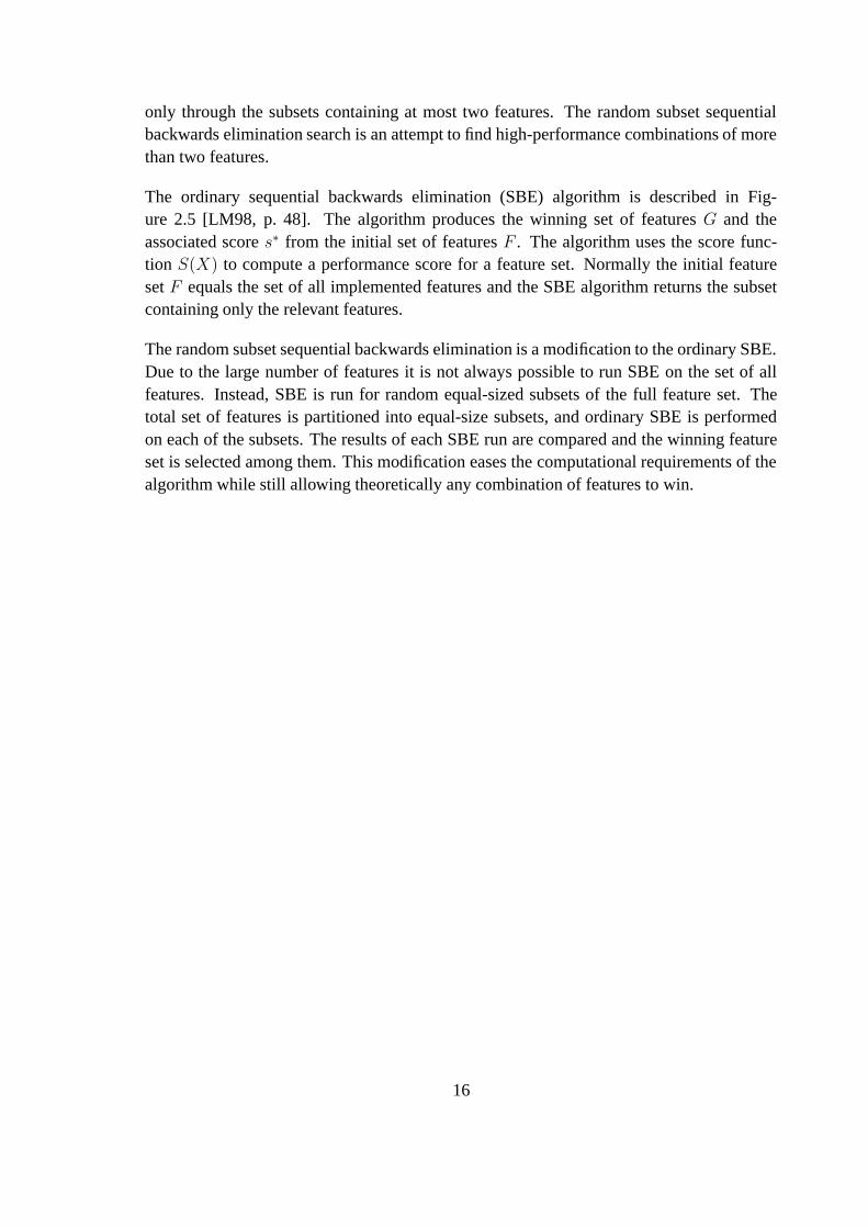
only through the subsets containing at most two features. The random subset sequentialbackwards elimination search is an attempt to find high-performance combinations of morethan two features.

The ordinary sequential backwards elimination (SBE) algorithm is described in Fig-ure 2.5 [LM98, p. 48]. The algorithm produces the winning set of features G and theassociated score s∗ from the initial set of features F . The algorithm uses the score func-tion S(X) to compute a performance score for a feature set. Normally the initial featureset F equals the set of all implemented features and the SBE algorithm returns the subsetcontaining only the relevant features.

The random subset sequential backwards elimination is a modification to the ordinary SBE.Due to the large number of features it is not always possible to run SBE on the set of allfeatures. Instead, SBE is run for random equal-sized subsets of the full feature set. Thetotal set of features is partitioned into equal-size subsets, and ordinary SBE is performedon each of the subsets. The results of each SBE run are compared and the winning featureset is selected among them. This modification eases the computational requirements of thealgorithm while still allowing theoretically any combination of features to win.

16

3 Previous models

This section contains a review of the most relevant previously published models on musicalmeter and beat recognition. Most of the models do not attempt to recognize meter on otherlevels than the beat. Such models are called beat trackers [AD90].

The extraction of two or more levels of metrical structure from an acoustic signal of musichas not been discussed per se in any previous literature. Furthermore, explicit estimationof the tatum from a musical signal, given no prior information, has only been describedin [Sep01] before. On the other hand, several reports describe a system for doing metricalanalysis from MIDI or some other symbolic representation. Methods operating purely onsymbols are more developed and claim to extract various sorts of high-level informationfrom a symbolic input. At the same time the audio signal processing models struggle evento find the beat robustly. There is an obvious dichotomy between the models that canprocess acoustic signals and the models that cannot.

Of the models presented below, Lee, Parncutt, Rosenthal, Temperley–Sleator and Toivi-ainen are the only actual meter models, i.e., models which observe more than just the beat.The other models concentrate on finding the beat. The meter models mentioned above arecapable of producing the tatum as a by-product. In a related thesis, Bilmes discusses an al-gorithm for creating a tatum grid that matches a score with a performance, given completemetrical knowledge of the piece [Bil93a].

The most important differentiator of the published models is the fact whether they takeacoustic signals or a symbolic representation such as MIDI as input. Scheirer argues contro-versially that pure symbolic note processing algorithms are only good for that one purpose,i.e., for processing notes symbolically, and they should not be applied to real-world musicalsignal analysis [Sch00]. I am inclined to agree, since very few symbolic algorithms havebeen successfully applied to real-world signal analysis, according to the literature. Dixonmakes an exception by proposing a symbolic MIDI beat tracker that can also be applied tosignal analysis [Dix01a]. However, there is a fine line between signal-processing and sym-bolic systems because beats are symbols. Since every (acoustic) beat tracker is an explicitsignal-to-symbolic transform, there is not much sense in differentiating ‘mostly symbolic’systems from ‘mostly signal processing’ systems.

Another important property of especially the beat tracking models is causality, that is,whether the model requires looking at input beyond current output point, in anticipation,or whether it does not. Humans always listen to music in real time, and therefore modelsthat ‘look into the future’ are not actually prospective models of music perception. Conse-quently, the primary goal of beat and meter recognition models is to perform equally well

17

as humans, in real time.6 Only after this are noncausal extensions justified. The publishedmodels can be divided according to these properties as

1. causal (non-anticipating) models processing acoustic audio signals: Goto–Muraoka [GM98], Scheirer [Sch98b];

2. noncausal models processing audio signals: Dixon [Dix01a], Foote–Uchihashi [FU01],Laroche [Lar01], Muscle Fish [WBKW96], Sethares–Staley [SS01], Tzanetakis–Essl–Cook [TEC01]; and

3. models processing symbolic data: Allen–Dannenberg [AD90], Brown [Bro93],Cemgil–Kappen–Desain–Honing [CKDH01], Eck [Eck01], Large–Kolen [LK94],Lee [Lee91], Parncutt [Par94], Povel–Essens [PE85], Raphael [Rap01], Rosen-thal [Ros92], Smith [Smi99], Temperley–Sleator [TS99], and Toiviainen [Toi97].

Above, I have not divided the non-acoustic models according to causality, due to the factthat the publications do not usually consider causality at all. Most of the symbolic modelsrequire access to the whole score of a piece of music, and would thus classify as noncausal.

I will now briefly summarize each of the above models. Due to the number of models, theyare presented in five qualitative categories:

1. rule-based search models,2. multiple-agent models,3. multiple-oscillator models,4. procedural models, and5. probabilistic models.

It should be noted that this categorization is ambiguous to a certain degree; especially therule-based search and multiple-agent model categories overlap.

3.1 Rule-based search models

The modeling of rhythm and meter perception started with rule-driven models capable ofprocessing simple notated monophonic melodies and rhythm patterns. The modeling wasdone in parallel with the research on defining the structure of rhythm. Rhythmic experi-ments served both the modeling work and the rhythm structure research.

Povel and Essens proposed one of the first computational models of rhythm perception.They describe a symbolic algorithm which processes periodic rhythmic onset sequences,assigning accents to onsets and finding the period and phase of an isochronous pulse that

6It is hypothesized that humans would alter earlier percepts in retrospect, based on later input. In effect,

this would have to be simulated noncausally, but only within the span of the perceptual present of approxi-

mately 4 seconds [Par94].

18

has the least counterevidence in the form of coinciding with non-accentuated onsets or withno onsets at all. The assignment of accents and the computation of counterevidence areguided by simple heuristic rules. [PE85]

The Lee model. A rule-based model that concludes the work of Longuet-Higgins andLee is published in [Lee91]. Lee’s symbolic model also handles counterevidence againstdifferent pulse hypotheses and works out the ‘least-unexpected’ pulses from onset timings.The model is sophisticated in that it attempts to recognize the metrical structure on morethan one level. Akin to Povel and Essens [PE85], Lee sets forth heuristic rules that drivethe model. [Lee91]

Parncutt brings two important features to his symbolic model in comparison to the previ-ous models: phenomenal accents and the preference for moderate tempo. Parncutt definesa phenomenal accent measure as the sum of terms measuring durational accent, loudnessaccent, pitch accent and possible interactions of these. In his model, however, he only usesand concretizes durational accent. He presents a model with a direct relationship betweeninter-onset intervals, durational accents, moderate tempo, and the perceived beat. In ad-dition to the beat, Parncutt’s model also estimates perceived meter, metrical accents, andexpressive timing information. [Par94]

The Temperley–Sleator model. Recently, Temperley and Sleator published a hybrid har-mony/meter recognition model that is also based on the rule-based search concept. The au-thors enumerate a set of rules which, for the meter part, draw heavily on Lerdahl and Jack-endoff [LJ83]. Similarly to the heuristics of the other models, the rules specify e.g. thatbeats should be spaced regularly, beats should align with onsets, and strong beats shouldalign with onsets of longer events. A score value is computed as a function of time, basedon the fulfillment of the above rules, and the meter is recognized from the scores withthe Viterbi algorithm. The Temperley–Sleator model is one of the models that produce ametrical grid with several levels. The model operates on symbols. [TS99]

Laroche proposes a beat tracking model for working with acoustic signals with a constanttempo. Furthermore, he assumes that every beat is divided into four tatums and that thesecond and fourth tatums may be delayed by an equal amount, corresponding to a typeof rhythm known as swing or shuffle. The onset detector is similar to that of Scheirer’sor Sethares’s and Staley’s, alhough Laroche does not reveal the number of bands he uses.The actual beat tracking model expresses the likelihood of onset locations with a four-component Gaussian mixture, where each component is centered at each tatum and findsthe maximum likelihood parameters by exhaustive search. [Lar01]

19

3.2 Multiple-agent models

The multiple-agent beat and meter recognition models all operate according to the sameprinciple. A number of differing hypotheses about pulse period and phase are made anda salience value is iteratively computed for each hypothesis. Each hypothesis is called anagent. In the course of tracking, hypotheses can be pruned or split, resulting in fewer ormore agents after that point. Hypothesis salience is increased whenever an onset coincideswith a pulse belonging to the hypothesis. More sophisticated models estimate the accen-tuation of notes and incorporate that into hypothesis salience computation. In the end, themost salient hypothesis is considered to represent the correct meter. One peculiarity of themultiple agent framework is the need for initialization; at startup, a sufficient number ofpotential hypotheses needs to be constructed. Different literature suggest different meansfor initializing the set of hypotheses.

Allen and Dannenberg were perhaps the first to construct a multiple-agent beat trackingmodel. Allen and Dannenberg lay a set of heuristic rules that penalize e.g. beats thathave a short note or no note at all, and then use beam search to find the most salient beattranscription. The algorithm is not completely autonomous because it needs to be given theinitial downbeat to start the search with, i.e., the initialization of hypotheses is the user’sresponsibility. The model processes MIDI. [AD90]

Rosenthal formulated a complete symbolic meter analysis system for polyphonic musicin his Ph.D. thesis. The model attempts auditory streaming by labeling incoming notes tomelody and chords, which then constitute the input to meter recognition. At startup, themodel considers the beginning of the musical piece and attempts to find the beat from that.This is accomplished by (1) computing an IOI histogram from the onsets in the beginning,(2) performing a harmonic transform to it,7 (3) convolving the result with a Gaussian func-tion, (4) weighting with an a priori tempo distribution, and finally, (5) by selecting theperiod corresponding to the maximum of the resulting function as the beat period. The beatand its subdivisions and multiples are then used to construct the initial hypotheses prior tobeam search through the piece. During the search, accentuation consisting of duration andthe existence and number of nearby onsets is attributed to onset events. [Ros92]

Goto and Muraoka have a series of publications on beat tracking, and their latest model isbest summarized in [GM98]. Their model operates on acoustic music signals by performingonset detection from the spectrogram of the incoming signal. Onset detection is performedindependently on multiple frequency bands and the authors assign agents to operate strictlyon the onsets coming from a specific frequency band. Each frequency band feeds multi-ple agents to facilitate multiple different meter hypotheses. The agents compute an IOIhistogram and determine the beat period based on that. Moreover, bass and snare drum

7Harmonic transform of a histogram p(x) is defined by ph(x) =∑

i wip(ix), which reinforces the re-

sponse at x by the responses at integral multiples of x according to weights w i. In [Ros92], ∀ i > 3 : wi = 0.

20

onsets are separated from the music and they are used as additional clues in beat detection.Detected bass and snare drum timing patterns are compared to internal rhythmic patternsto distinguish strong and weak beats. The publication does not reveal how hypotheses areinitialized in the model. [GM98]

Dixon has presented a noncausal multiple-agent beat tracking algorithm. Dixon’s modelis capable of processing acoustic musical signals in addition to symbolic data. At first, thesystems performs a coarse sound onset detection to the audio signal by applying a high-passfilter, full-wave rectifier and a moving average filter in cascade, and then picking peaks fromthe resulting power signal. Inter-onset intervals (IOI) are clustered into a histogram-alike“class” representation, where each IOI belongs to one class and the populations of IOI’sin each class are computed. The beat period hypotheses are initialized as in Rosenthal’smethod. The actual beat positions are found by an iterative search through the onsets.A worthwhile remark of the model is that it in no way takes explicit advantage of anyacoustic (phenomenal) accent information.8 [Dix01a]

3.3 Multiple-oscillator models

An oscillator is a concrete parametric model of pulse generation, and therefore it wouldseem natural to simulate pulse reception with a phase-locking oscillator. This has indeedbeen pursued in a number of publications, each concentrating on a different problem do-main, oscillator type or oscillator network formulation. Multiple copies of the basic oscilla-tor are used in the models to account for different meter hypotheses; a single basic oscillatoronly responds at a characteristic frequency range.

The oscillators need to be stimulated with a train of impulses or some other sort of impulsiveexcitation. If the period of the excitation matches the characteristic frequency of a givenoscillator, the oscillator will start to converge towards oscillating in unison with the excita-tion. Thus, a bank of oscillators is constructed, consisting of several oscillator units withnonoverlapping frequency ranges, together spanning a rhythmic frequency range. Then,during meter recognition, the degree of resonance of each oscillator is observed, and theoutput of the strongest-resonating oscillator is chosen as the recognized pulse.

The Large–Kolen model is one of the first models to use oscillator units for representingmeter perception. The authors describe a nonlinear oscillator unit that, when stimulatedwith a pulse train within its characteristic frequency range, responds with synchronizedpulsation. When the oscillators are arranged into a bank of six oscillators in parallel andfed an identical pulse train, some of the oscillators synchronize with different metrical levelsof the input, while others fail to synchronize at all. The model is symbolic. [LK94]

8Dixon remarks that the simplistic onset detector can be regarded as a filter of non-accentuated events.

21

Toiviainen has developed an oscillator bank for the recognition of meter [Toi97] and ap-plied it to automatic accompaniment of piano playing [Toi98]. The nonlinear oscillators aresimilar to those of Large and Kolen. The model consists of two oscillator banks, the firstfor beat tracking and the second for tracking the next-highest metrical level. The output ofeach oscillator in the first bank is connected to a pool of oscillators in the second bank. Theresonant frequencies of the second bank are tuned to two and three times that of the firstoscillator, to facilitate for binary and ternary meters. The model consumes MIDI. [Toi97]

The Scheirer model. The algorithm proposed by Scheirer is a causal, or non-anticipating,signal processing model of beat tracking from an acoustic input signal. The model is rootedin a subband front-end inspection of the musical signal, aiming to produce a perceptuallyrelevant amplitude envelope representation at each frequency band. The beat tracking iscarried out with an independent oscillator bank on each subband, and the final beat trackingresult is combined based on the energies of the subband oscillators. Each subband oscil-lator bank contains oscillators with identical characteristic frequencies, and the energies ofidentical oscillators are summed across bands. Scheirer introduced the idea of using combfilters as oscillator units, with the benefit that a comb filter oscillator will resonate at integralmultiples of its characteristic frequency. Thus an oscillator will start to follow rhythms thatcorrespond to its characteristic metrical level and all sublevels of it. [Sch98b] [Sch00]

Eck has built a symbolic model from neurologically motivated oscillator units calledFitzhugh–Nagumo relaxation oscillators. The type of oscillator was originally designedto model the dynamics of neural action potential. Eck builds a network of 20 oscillators,where every oscillator is coupled with all the other oscillators through a specific couplingfunction. This model is clearly the most complex of the multiple-oscillator models. [Eck01]

3.4 Procedural models

The procedural models can not be characterized with a common property, they are onlysimilar in that they can be described only through the procedure they follow. In most of thecases this means the application of a standard signal processing method to beat tracking.

Brown describes the use of autocorrelation for simple metrical analysis. Her work isbased on finding the inherent pulsation of an onset stream by finding a lag for which theautocorrelation is high. The onset stream is represented as an (irregular) pulse train. [Bro93]

The Muscle Fish content-based audio retrieval system features a simple beat trackingsubsystem based on a “bass loudness time series” analysis. They perform the FFT on theamplitude envelope of low-pass filtered acoustic music signal and pick the FFT frequencybin with the most energy. Consequently, the system cannot infer anything from high-passsignals. [WBKW96] [BKWW99]

22

Smith proposes the application of the wavelet transform for beat tracking. In a similar wayas Brown, he first constructs a pulse train signal from a list of symbolic onset times. Thepulse train signal is then decomposed with the Morlet continuous wavelet transform intoa time-frequency representation. Subsequent processing in the time-frequency domain isthen performed to reveal the beat. [Smi99]

Foote and Uchihashi have applied an audio self-similarity concept for beat tracking. Thealgorithm consists of extracting spectral features from the audio signal, computing a sim-ilarity metric between all pairs of feature vectors, and finally taking an autocorrelation ofthe similarity data. The beat period is the lag of the highest autocorrelation peak. Due tothe computation of the autocorrelation over the entire audio sample, the algorithm is notcausal. The most important contribution of this article is the proposition to use a similaritymetric between two points in the audio signal to determine the beat period, rather than toestablish the accentuation in a single point. The other reviewed audio processing modelsrely on trying to measure the phenomenal accent of a single point in the signal, i.e., whethera single point is a beat in itself or not. [FU01]

Tzanetakis, Essl, and Cook have developed an acoustic beat tracking subsystem to a mu-sical genre recognition system. The beat tracker has a four-band preprocessing stage con-sisting of octave-band wavelet analysis, rectification, low-pass filtering, decimation, nor-malization, and summation across bands. Beats are computed from this excitation signalwith autocorrelation, in a noncausal fashion. [TEC01]

The Sethares–Staley model uses the periodicity transform for beat tracking. The model issuited to processing of acoustic music signals through the pre-processor, which in practiceis very much alike the front end of Scheirer’s model. The incoming signal is transformedto frequency domain with the FFT, parted into 23 frequency bands, whose RMS amplitudeenvelopes are then computed. Next, the amplitude envelope of each band is transformed toperiodicity domain with the novel periodicity transform, in which the highest value is thenselected. [SS01]

3.5 Probabilistic models

Probabilistic models do not share a similar structure but a similar modeling approach. Theview behind probabilistic models is that onset times and other acoustic phenomena areactually random by nature, and the observations are contaminated with uncertainty. Proba-bilistic models attempt to tackle the uncertainty by including it in the model. The proposedmodel also attempts to leverage probabilistic methods in its processing.

The Cemgil–Kappen–Desain–Honing model. The recent approach to beat tracking byCemgil et al. draws from the body of statistical modeling research and from the theory

23

of linear dynamical systems in particular. It has been previously assumed that the timingdeviations in piano playing obey the Gaussian probability distribution [Sch95, p. 45], butvirtually no usage has been made of this prior to this model. Cemgil et al. estimate thebeat trajectory by applying a Kalman filter to the output of a local periodicity data they callthe tempogram. The Kalman filter optimizes the parameters of a linear dynamical system,where the beat position and the logarithm of beat period are hidden variables [GH96]. As aresult, estimates of beat positions are produced. The tempogram periodicity data representsenergy as a function of period in a local timeframe. The function resembles an IOI his-togram with memory but tolerates deviations in onset times in a configurable amount. Themodel processes MIDI data. [CKDH01]

Raphael constructs a Bayesian belief network for simultaneous tracking of beats and quan-tization of notes from a symbolic onset stream. His method requires that the possible posi-tions of onsets within a measure are known a priori. Once this is known, the belief networkmodels the relationship of the discrete measure positions to a continuous tempo functionand further to the continuous observed onset times. The tempo and onset quantization re-sults are then given by maximum a posteriori (MAP) estimation. [Rap01]

3.6 Commercial systems

This section contains a brief summary of the advertised features and the actual performanceof a sample of the currently available commercial solutions for beat tracking. Currently, nocommercial solutions exist for meter recognition.

Native Instruments Traktor software. This program performs real-time beat trackingfrom acoustic input. The incorporated model would seem to respond only to low-frequencycontent and thus I believe it to be similar to the Muscle Fish “bass loudness time seriesanalysis” procedural approach. [Ins01]

Sonic Foundry Acid Pro 3 software. This software carries out a noncausal analysis of anacoustic audio signal. In the course of the analysis, the user is asked to verify the decisionsmade by the algorithm. Based on user feedback, the software attempts to position the beatsand the measures. The approach taken seems to be a heuristic search, in which a regulargrid is matched which the transients in the input signal. [Fou01]

DJ hardware. Several pieces of hardware possess a tempo recognition feature. Accordingto my experience, they however unanimously respond only to low-frequency content. Thebass loudness time series analysis behaves similarly in this respect, which would imply thata simplified variant of it would be used.

E-mu sampler hardware. The latest sampler models of E-mu incorporate a version of theLaroche beat tracker. The main operation of the model is summarized above. [Sys99]

24

4 Proposed model

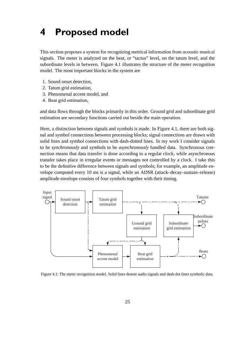
This section proposes a system for recognizing metrical information from acoustic musicalsignals. The meter is analyzed on the beat, or “tactus” level, on the tatum level, and thesubordinate levels in between. Figure 4.1 illustrates the structure of the meter recognitionmodel. The most important blocks in the system are

1. Sound onset detection,2. Tatum grid estimation,3. Phenomenal accent model, and4. Beat grid estimation,

and data flows through the blocks primarily in this order. Ground grid and subordinate gridestimation are secondary functions carried out beside the main operation.

Here, a distinction between signals and symbols is made. In Figure 4.1, there are both sig-nal and symbol connections between processing blocks; signal connections are drawn withsolid lines and symbol connections with dash-dotted lines. In my work I consider signalsto be synchronously and symbols to be asynchronously handled data. Synchronous con-nection means that data transfer is done according to a regular clock, while asynchronoustransfer takes place in irregular events or messages not controlled by a clock. I take thisto be the definitive difference between signals and symbols; for example, an amplitude en-velope computed every 10 ms is a signal, while an ADSR (attack–decay–sustain–release)amplitude envelope consists of four symbols together with their timing.

Sound onsetdetection

Tatum gridestimation

Phenomenalaccent model

Beat gridestimation

Subordinategrid estimation

Inputsignal

Ground gridestimation

Tatums

Subordinatepulses

Beats

Figure 4.1: The meter recognition model. Solid lines denote audio signals and dash-dot lines symbolic data.

25

Prior to metrical analysis, the audio signal is preprocessed with a sound onset detector.The onset detector tracks changes in the root-mean-square (RMS) amplitude envelope onmultiple frequency bands and emits onset events at points of rapid level increase. Theonset detector transforms the audio signal into a symbolic representation consisting of onsettimes, amplitudes, spectral location, etc.

Next, the tatum estimator processes the stream of onsets causally, enabling the trackingof accelerandos and ritardandos by using an exponentially decaying window for past data.Rubatos and tempo changes are detected after a latency time dictated by the observationwindow length. The tatum estimator outputs the tatum pulse, which enables synchroniza-tion to the stream of onsets and thus to the audio signal itself. A stabilized version of thetatum is produced by removing discontinuities from the tatum period. In this work, thestabilized pulse is termed the metrical ground. It is then used internally in the model tosegment the audio signal.

Then, each element in the segmented audio signal is fed to the phenomenal accent model,which measures psychoacoustic accentuation at that point in the signal. The model oper-ates by computing acoustic features such as onset power, onset spectral shape, bass leveletc. from the signal and then projecting the feature values into an estimate of phenomenalaccentuation.

Finally, the beats are found based on the phenomenal accents and the ground-level pulse.The beat estimator observes the stream of phenomenal accents for periodicities near100 BPM. It is working causally, too, making the recognition of sudden tempo changespossible. The beat estimator outputs a pulse on every beat. For completeness, the pulses onsubordinate metrical levels between the beat and the tatum are filled in. This can be donebased on knowledge of the tatum and the beat.

As concluded in Section 3, the only viable models of meter perception are causal. There-fore, while this model attempts to mimic the behavior of human meter perception, it alsohas to be causal. The process in Figure 4.1 is functioning continuously when music is beinganalyzed, and the outputs track the input with a delay.

4.1 Sound onset detection

Reliable detection of real note and sound onsets from an acoustic waveform is a very chal-lenging task. Sound onset detectors have been built for the purposes of automatic musictranscription [Sch85] [CJK+85] [Kla98], computational auditory scene analysis [BC94],and of course musical meter analysis [Tod94] [GM98] [Smi99]. The task of precisely find-ing sound onset points is akin to making a transcription of the piece of music, which stillin general remains an unsolved problem in the case of polyphonic music. It is also debated

26

Inputsignal

BPF

Attacktime

8 bands

RegistralIOI

Amplitude

Combinationacrossbands Onset times

Amplitudes

Registral IOI's

Attack times

Band centroids

Raw onsetdetector

Onset times

Bandwidths

Amplitudeenvelope

Figure 4.2: The onset detector. The blocks apart from the across-band combiner are identical for all eightbands.

whether onset detection should even be attempted in the first place. Scheirer criticizesthe efforts to first encode information using notes within a musical analysis system andthen to process them using a high-level symbolic musical analyzer. He opposes symbolicnote data because of the limitations in onset detection, but more importantly because ofthe implied proposition that human perception would be transcribing notes as we listen tomusic [Sch00].

Yet sound onset detection becomes practicable if we loosen the requirements of finding ab-solutely correct note onset data and instead concentrate on finding only the most obviousnote onsets. Such an onset detector would not fulfill the promise of an automatic musictranscription system, but here it provides the necessary amount of information for the sub-sequent processing stages to find implied pulsations.

Figure 4.2 shows an overview of the onset detector. The incoming music signal is dividedinto individual frequency bands with eight parallel band-pass filters (BPF). Then, on eachfrequency band, raw onsets are detected simply by looking for rapid increases in the band-wise amplitude envelope. For each detected raw onset, further data is computed on a singlefrequency band. Finally, all the raw onsets together with accompanying data from all eightbands are inspected together to combine simultaneously occurring raw onsets into one.

Previous onset detection algorithms are mostly based on first estimating the amplitude en-velope of the audio signal and then thresholding the first-order difference of the amplitudeenvelope to find onsets. In contrast to them, the raw onset detector described in Figure 4.3gains an advantage by combining multiband analysis and the nonlinear difference func-tion (xn − xn−1)/(xn + xn−1). This overall approach was originally proposed by Klapuriin [Kla99].

27

Half-Hanning

Band-passsignal

LPF

1

1

-

-

+

-

nn

nn

xx

xx

),0max( x2x x

RMS estimation

441

Thres-holding

Channelamplitudeenvelope

Channelraw onsets

Delay

Figure 4.3: The detector of bandwise raw onsets. The processing is duplicated for all channels identicallyexcept for the Delay block.

Table 4.1: Onset filterbank analysis filter passband frequencies, bandwidths, and compensation delays. Thedelays are computed from mean filter passband group delays.

Number Passband Bandwidth (hertz) (octaves) Delay1 50–106 Hz 55.9 Hz 1.08 0 ms2 106–224 Hz 119 Hz 1.08 7.21 ms3 224–476 Hz 251 Hz 1.08 10.6 ms4 476–1010 Hz 532 Hz 1.08 12.1 ms5 1010–2140 Hz 1130 Hz 1.08 12.9 ms6 2140–4530 Hz 2390 Hz 1.08 13.2 ms7 4530–9590 Hz 5060 Hz 1.08 13.4 ms8 9590–20300 Hz 10700 Hz 1.08 13.5 ms

4.1.1 Filterbank analysis

Sound onsets are observed on eight non-overlapping frequency bands, distributed logarith-mically from 50 Hz to 20 kHz. The number of frequency bands used has varied quitemuch in the literature: some naïve approaches use a single bass band below approximately100 Hz [WBKW96], while others use a single treble band above 1 kHz [Bil93b] [Dix01a],Scheirer has used six [Sch98b], Klapuri 21 [Kla99], Sethares and Staley 23 [SS01], Cari-ani 25 [Car01] and Smith as many as 28 non-overlapping bands [Smi96]. The number andlogarithmic positioning of the analysis filters in this work are motivated by psychoacous-tics [ZF90] and auditory models [Sla93].

Filter linear phase response has been compromized in favor of more efficient computationthrough the use of sixth-order Butterworth IIR (infinite impulse response) filters. For com-parison, the gammatone filters in an auditory model are eight-order IIR filters [Sla93].

28

Figure 4.4: Onset filterbank analysis filter responses. Odd-numbered filter responses are drawn with solidcurves, while even-numbered responses have dashed response curves.

The actual filter design parameters, consisting of filter cut-off frequencies, are listed in Ta-ble 4.1. The table lists also filter passband bandwidths and required delay compensations,computed from passband group delay means [OS89]. The additional delay in Figure 4.3is necessary to compensate for the different group delays of the analysis filters. Withoutcompensation, the raw onsets of a single musical event would not coincide between bands.All the eight analysis filters have a 13-semitone (1 and 1/12-octave) bandwidth, i.e., thebandwidths in hertz are different between filters and grow exponentially from lower bandstowards upper bands. Filter amplitude responses are illustrated in Figure 4.4. The filter-bank is called a constant-Q filterbank, since the filter bandwidths are proportional to filterpassband center frequencies. Therefore the input signal producing equal power output fromall filters is pink noise, i.e., noise with a 1/f power spectral density.

4.1.2 Channel amplitude envelope

As show in the diagram in Figure 4.2, the input signal is filtered in parallel with each of theeight band-pass filters. On each band, this produces a subband signal s[n] — in this simpli-fied notation the subband number is not explicitly written. After separating the frequencybands, the root-mean-square (RMS) level of each subband signal s[n] is estimated using

r[n] =√

g[n] ∗ (s[n]2), (14)

where g[n] is a third-order Butterworth IIR low-pass filter (LPF) cutting off at approxi-mately 30 Hz. The RMS signal r[n] is a positive-valued signal which serves as a good

29

estimate of the short-time power present on the band at each time. Because r[n] containsvery little energy above 50 Hz, it is decimated to a sample rate of 100 Hz to remove theoverhead from forthcoming computations. In the passband 0–30 Hz, the RMS low-passfilter g[n] introduces a group delay of 8.3 ms ± 0.8 ms, and thus the phase response can besaid to be approximately linear for practical purposes.

Next, in simple imitation of the human auditory system, the amplitude envelope a[n] iscomputed from the decimated RMS signal by convolving it with a 100 ms half of a raisedcosine (also termed von Hann and hanning) window. The motivation for this is that thehalf-hanning window performs temporal integration like the auditory system and effectivelymasks rapid amplitude modulation [Tod94]. This window has a deliberately nonlinear phaseresponse whereby low frequencies are significantly delayed (approximately 25 ms below5 Hz) and higher frequencies are slightly advanced (about 13 ms around 14 Hz and about5 ms above 20 Hz). From the two filters, the half-Hanning filter is more dominant on phaseresponse, while both the filters contribute to the amplitude response.

4.1.3 Amplitude envelope thresholding

An approximate formula for detecting noticeable sound onsets from the amplitude envelopecan be devised by starting from the Weber fraction ∆I/I , where ∆I is the just-noticeabledifference (JND) in sound intensity and I is the intensity of the reference sound [Kla99].Since, by assumption, for wideband signals this fraction is constant, k = ∆I/I , we canexpress the intensity JND as a function of reference intensity ∆I = kI [AN97]. Whiledoing raw onset detection, we observe the change of sound intensity between one timeinstant, I[n − 1], and the next, I[n], and we wish to compare the change in intensity withthe intensity JND,

I[n]− I[n− 1] ≥ kI[n− 1] ⇐⇒ I[n]− I[n− 1]I[n− 1] ≥ k. (15)

Given that sound intensity is proportional to power, I ∝ a2 [AN97], we geta[n]2 − a[n− 1]2

a[n− 1]2 =a[n]− a[n− 1]

a[n− 1]a[n] + a[n− 1]

a[n− 1]︸ ︷︷ ︸≈2

≥ k. (16)

In practice, it turns out that the second factor in Equation (16) can be well replaced with aconstant of two without causing any significant change in the value of the function. In effectthis implies that the time step is small enough to make the change in intensity very little,I[n− 1] ≈ I[n]. This yields

a[n]− a[n− 1]a[n− 1] ≥ k

2, (17)

and by estimating the denominator with the mean of a[n − 1] and a[n] we get a slightincrease in robustness, yielding

b[n] =a[n]− a[n− 1]a[n] + a[n− 1] ≥

k

4≈ 0.06, (18)

30

where k = ∆I/I = 10−6/10 for wideband noise according to Plack and Carlyon [PC95,pp. 134–135].

Therefore, the detection of raw sound onsets from the amplitude envelope a[n] is done bycomparing the relative difference b[n] to the constant (upper) threshold 0.06. The pointwhere this threshold is exceeded is called the raw onset rise point. Starting from the risepoint, the increase in the amplitude envelope is attributed to a single raw onset up to the rawonset fall point where either (a) b[n] descends below a constant lower threshold,−0.035, or(b) 300 ms have passed. After this, the detection starts again, and b[n] is compared to theupper threshold for a new onset.

Raw onset amplitude ao is computed from the amplitude envelope during the attack of thesound, ao = a[nf ] − a[ni], nf > ni. The sound attack initial amplitude, a[ni], is takenfrom the first local minimum backwards from the onset rise point. The sound attack finalamplitude a[nf ] is the maximum amplitude encountered between the raw onset rise and fallpoints. Raw onset attack duration toa is computed from the initial and final attack pointtimes, toa = (nf − ni)/100 Hz.

4.1.4 Rough sound duration estimation

Raw sound duration is approximated by the within-band distance from one onset to the nextloud enough onset, which is called the registral inter-onset interval (registral IOI) [TS99].As discussed below, this does not equal sound duration, and sounds may well be bothshorter or longer than registral IOI’s. However, given the fact that obtaining accurate infor-mation on sound duration is very hard, the registral IOI provides a good guess of it.

For a raw onset at time t0, I define the registral IOI measure d > 0 with the equation∫ t0+d

t0

∑i

aif(t− ti) dt = 1, where (19)

f(t) =

{1

0.99pe−pt if t ≥ 0

0 otherwise.

Here {t0, t1, t2, . . .} are the times and {a0, a1, a2, . . .} are the amplitudes of raw onsets ona single frequency band. The parameter p = −(ln 0.01)/dmax controls the compactness ofthe onset response according to the upper registral IOI limit dmax. Integrating Equation (19)yields the implementable formula∑

i

aig(d− ti) = 1, where (20)

g(t) =

{1

0.99(1− e−pt) if t ≥ 0

0 otherwise.

Equation (20) incorporates a model of sound duration, according to which a sound is con-sidered to continue sounding only up to a following onset with an amplitude equal to (or

31

greater than) the amplitude of the previous sound. All following onsets that are distinctlyquieter than the sound under observation do not affect the duration much. Nevertheless, if asufficient-amplitude onset does not follow the given onset, IOI values are bounded to dmax

from upwards.

4.1.5 Combining bandwise raw onsets

After detecting raw onsets independently on each frequency band, the final set of onsets isproduced from the raw subband onsets, excluding distinctly low-amplitude onsets. The rawonsets whose amplitudes are below the 10th percentile (0.1th quantile) of all amplitudes arediscarded.

Onset aggregation is done based on a minimum allowed inter-onset distance of 60 ms,which is an estimate of the minimum discriminable IOI [Par94]. All raw onsets within the60 ms range are combined into a single genuine onset, whose time is the median of thetimes of the raw onsets; median is used instead of mean in order to suppress the effect ofoutliers. Raw onset amplitudes combine with summation. The attack time of the combinedonset equals the mean of the attack times of the corresponding raw onsets and the aggregateregistral IOI equals the maximum of the raw onsets’ registral IOI’s.

4.2 Tatum grid estimation

The aim of tatum period estimation is to estimate the average interval between successivepulses on the lowest metrical level. This will be denoted q. The tatum period q is estimatedcausally, from incoming onsets one at a time, resulting in a time-varying estimate of it.9

The only information used to determine the tatum period are the times of the onsets, dis-carding all information of the pitch, timbre and loudness of the musical signal. Preliminaryexperiments indicate that incorporating loudness or any other auxillary information into thetatum estimation process will more likely produce a false tatum. This observation seemsrather logical, considering the fact that the loudness or timbre of onsets tend to correlatemore strongly at the beat level than at lower metrical levels [LJ83].

4.2.1 Inter-onset interval computation

The onset stream is first transformed into inter-onset interval (IOI) data. Given two onsetsat times ta and tb, ta < tb, the IOI between the onsets is defined as o = tb − ta. The IOI’sare not only computed between pairs of successive onsets; rather, all onset pairs whose

9Most of the contents in this section has been published also as a separate paper [Sep01].

32

0 0.4 0.8 1.20

0.5

1

1.5

2(h1)

IOI [s]

Rat

e [1

/s]

0 0.4 0.8 1.20

0.5

1

1.5

2(h2)

IOI [s]100 200 300

0.04

0.06

0.08

0.1

0.12

(e1)

Period [ms]

RE

F

100 200 300

0.04

0.06

0.08

0.1

0.12

(e2)

Period [ms]

Figure 4.5: Accumulated IOI histograms (h1) and (h2) and REF’s (e1) and (e2) of the example signals after10 seconds of processing. The signals are excerpts from (1) “Da Sambafrique” by Nick Holder (instrumentalhouse music) and (2) “Segue o Seco” by Marisa Monte (live performance of brazilian pop music). Detectedtatums are 120 ms and 181 ms, respectively.

IOI’s are within an upper limit are taken into account. This procedure (also used by Rosen-thal [Ros92] and Dixon [Dix01a]) is a variation of the conventional notion of the IOI.10

4.2.2 Greatest common divisor approximation

If we assume that there are no random deviations in the IOI values, the IOI’s are all exactintegral multiples of the tatum, implying that the tatum is equal to the greatest commondivisor (GCD) of the IOI’s. I now introduce a scheme to estimate the GCD in a situationwhere the IOI’s contain random deviations.

Let us define a remainder error function (REF), as a function of period p and inter-onsetintervals oi:

e(p) =n∑

i=1

(oip−⌊oip+1

2

⌋)2

. (21)

The local minima of Equation (21) represent possible tatum candidates. If an exactGCD exists, it can be found by finding the greatest value for which the REF is zero, orgcd(o1, o2, . . . , on) = max {p | e(p) = 0}.

4.2.3 Inter-onset interval histogram

In order for the algorithm to accommodate tatum changes (e.g. accelerandos and ritardan-dos), the IOI’s are converted into a time-varying histogram representation, accumulatedfrom onset to onset. Figure 4.5 illustrates example histograms of two music samples.

10The conventional IOI is the time difference between successive notes in monophonic melodies and

rhythm patterns.

33

Let h[k], 0 ≤ k ≤M−1, represent the contents of the M-bin IOI histogram. The histogramis constructed by counting the population of IOI’s oi discretized with a step size of r. Thiscontribution of the IOI’s for every new onset are gathered to a histogram fill function f [k] =

card ({i | (|oi − hx[k]| ≤ r)}), where hx[k] = kr are the histogram bin centers and card(·)denotes the cardinality, i.e., the number of elements in a set.

After discretization, the updated histogram h′[k] is computed by adding the fill functionf [k] to the past histogram h[k] to implement a leaky integrator,

h′[k] = clh[k] + cff [k], (22)

where the leak and fill coefficients are cl = 0.5tu/t1/2 and cf = (ln 2)/t1/2, where tu isthe time since last histogram update and t1/2 is the histogram content decay time constant.The coefficients cf and cl are variable, depending from tu, because the update rate is notconstant but dependent on onset rate. Using this weighting, the histogram represents theweighted average of the past IOI rate in terms of the average number of IOI’s per second.

The remainder error function (21) can be re-formulated for use with the IOI histogram andnormalized,

e(p) =

M−1∑k=0

h[k]

(hx[k]

p−⌊hx[k]

p+1

2

⌋)2/M−1∑k=0

h[k]. (23)

The histograms and remainder error functions computed with Equation (23) are illustratedin Figure 4.5.

4.2.4 Remainder error thresholding

After the computation of the remainder error function e(p), the tatum period must be cho-sen. According to the definition of the GCD, the tatum is the highest local minimum ofthe remainder error function. A parametrized threshold value eth = αminp e(p) + (1 −α)medianp e(p) is used to select the tatum q as the most prominent local minimum be-low the threshold. Here α = 0.4. Figures 4.5(e1) and 4.5(e2) show both the medians(dash-dot line) and the thresholds (dashed line) in addition to the remainder error functions(solid line).

4.2.5 Tatum phase estimation

The exact points of the tatum grid are positioned only after the tatum period has beencomputed, adapting the grid towards the actual onsets, since by assumption, all the observedonsets are on average aligned with the tatum grid [LJ83]. In the following, the position ofan individual tatum grid point is indicated by ϕ.

34

Figure 4.6: The tatum period (solid) and the ground period (dashed) as a function of time. The excerpt isa 15-second solo guitar sample from “Under the Bridge” by Red Hot Chili Peppers.

Given N onsets ti between two tatum grid points ti ∈ [ϕ, ϕ+ q], the average deviation δ ofthe onsets is given by the circular mean

δ =q

2π\

(1

N

N∑i=1

ej2π(ti−ϕ)/q

), (24)

where the angle operator \(·) gives the phase angle, within [−π, π), of its complex argu-ment. After the average deviation between the onsets and the grid is known, the positionof the next grid point ϕ′ is corrected to make the deviation smaller, parametrized with aconstant coefficient β = 0.1: ϕ′ = ϕ+ q + βδ.

4.2.6 Metrical ground estimation

The metrical ground is an artificial metrical level fabricated from the tatum. The metricalground is simply a cure to the problem of the tatum period exhibiting discontinuities andhopping from one metrical level to another. For example, the meter of a piece may changein a way that the tatum period changes from being half the beat period to being a fourth.Because of this difference the tatum grid cannot be used as a basis for comparing e.g.metrical distances before and after the change.

In addition to real changes in meter, the tatum period often contains spurious jumps toperiods in an integral relation. For example, in Figure 4.6, the tatum period oscillatesbetween 110 ms and 220 ms. These period changes are not necessarily errors, since thesignal is a demanding passage with solo electronic guitar playing.

The metrical ground grid is constructed by unwrapping the tatum period into a sublevel ofit near to 120 ms period. Every time there is a discontinuity in tatum period, the ratio oftatum period to ground period is updated so that the ground grid stays continuous by force.In the beginning of Figure 4.6, the tatum is 195 ms and the sublevel nearest to 120 ms is

35

195/2 ≈ 98 ms. Later, when the tatum period has a discontinuity, the ground period keepson the same level.

4.3 Phenomenal accent estimation

In order to build a metrical hierarchy on top of the tatum grid, there has to be a way todifferentiate between individual tatums. As laid out in Section 2.3, the pulse positions onall higher metrical levels are drawn from the set of pulse positions on the lowest level. Thismeans that it cannot be determined solely from the tatum grid whether a given grid pointis a beat or not, although all of the beats coincide exactly with a subset of the tatum gridpoints.

Tatum pulse positions are inspected and differentiated in a supervised pattern recognitionframework. In this framework, the acoustic signal in the neighborhood of each tatum gridpoint is inspected and characterized using a set of relevant features. These features are thenused as input to a statistical model together with the “ground truth” information of whethera single tatum is also a beat or not. The statistical model is supposed to learn the classesbased on the pure acoustic signal features.

Such a bottom-up model for recognizing beats cannot achieve a very high percentage ofdiscriminating beats from offbeats because the model in no way takes into account thetemporal regularity of beats. This bottom-up beat recognition model is therefore meantonly as a model of the phenomenal accentuation, i.e., objective acoustic evidence of abeat at a given observation point in music. The model attempts to incorporate most of theproperties of phenomenal accents, including

• sound onset times,• sound durations,• local emphasis of loudness or timbre, and• other sudden changes in loudness or timbre,

as given in Section 2.3. The aim of the phenomenal accent model is to produce a singlenormalized value representing the total phenomenal accentuation at the observation point.

4.3.1 Music corpus processing

In general, one needs loads of diverse and annotated data to carry out any kind of statisticalanalysis. In beat recognition, this means having a lot of songs with annotated beat posi-tions. The corpus collected in this work contains 330 musical signal excerpts; the beat ineach signal excerpt was manually annotated. The song names and other data are listed inAppendix A.

36

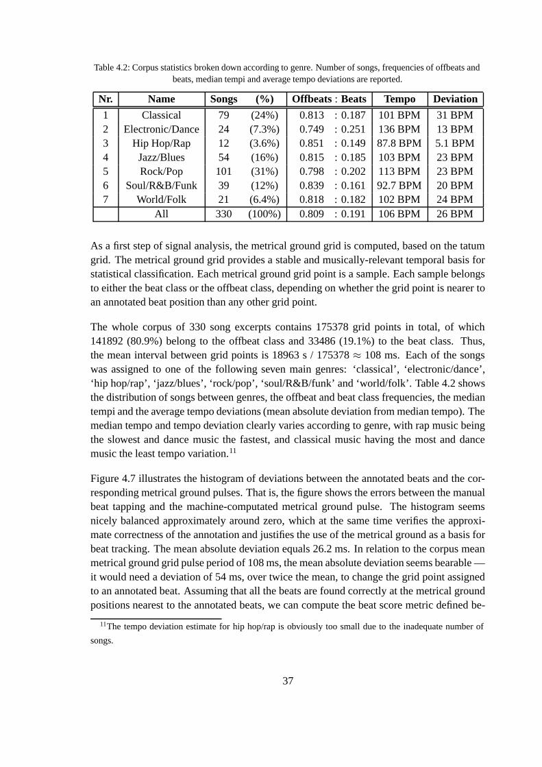
Table 4.2: Corpus statistics broken down according to genre. Number of songs, frequencies of offbeats andbeats, median tempi and average tempo deviations are reported.

Nr. Name Songs (%) Offbeats : Beats Tempo Deviation

1 Classical 79 (24%) 0.813 : 0.187 101 BPM 31 BPM2 Electronic/Dance 24 (7.3%) 0.749 : 0.251 136 BPM 13 BPM3 Hip Hop/Rap 12 (3.6%) 0.851 : 0.149 87.8 BPM 5.1 BPM4 Jazz/Blues 54 (16%) 0.815 : 0.185 103 BPM 23 BPM5 Rock/Pop 101 (31%) 0.798 : 0.202 113 BPM 23 BPM6 Soul/R&B/Funk 39 (12%) 0.839 : 0.161 92.7 BPM 20 BPM7 World/Folk 21 (6.4%) 0.818 : 0.182 102 BPM 24 BPM

All 330 (100%) 0.809 : 0.191 106 BPM 26 BPM

As a first step of signal analysis, the metrical ground grid is computed, based on the tatumgrid. The metrical ground grid provides a stable and musically-relevant temporal basis forstatistical classification. Each metrical ground grid point is a sample. Each sample belongsto either the beat class or the offbeat class, depending on whether the grid point is nearer toan annotated beat position than any other grid point.

The whole corpus of 330 song excerpts contains 175378 grid points in total, of which141892 (80.9%) belong to the offbeat class and 33486 (19.1%) to the beat class. Thus,the mean interval between grid points is 18963 s / 175378 ≈ 108 ms. Each of the songswas assigned to one of the following seven main genres: ‘classical’, ‘electronic/dance’,‘hip hop/rap’, ‘jazz/blues’, ‘rock/pop’, ‘soul/R&B/funk’ and ‘world/folk’. Table 4.2 showsthe distribution of songs between genres, the offbeat and beat class frequencies, the mediantempi and the average tempo deviations (mean absolute deviation from median tempo). Themedian tempo and tempo deviation clearly varies according to genre, with rap music beingthe slowest and dance music the fastest, and classical music having the most and dancemusic the least tempo variation.11

Figure 4.7 illustrates the histogram of deviations between the annotated beats and the cor-responding metrical ground pulses. That is, the figure shows the errors between the manualbeat tapping and the machine-computated metrical ground pulse. The histogram seemsnicely balanced approximately around zero, which at the same time verifies the approxi-mate correctness of the annotation and justifies the use of the metrical ground as a basis forbeat tracking. The mean absolute deviation equals 26.2 ms. In relation to the corpus meanmetrical ground grid pulse period of 108 ms, the mean absolute deviation seems bearable —it would need a deviation of 54 ms, over twice the mean, to change the grid point assignedto an annotated beat. Assuming that all the beats are found correctly at the metrical groundpositions nearest to the annotated beats, we can compute the beat score metric defined be-

11The tempo deviation estimate for hip hop/rap is obviously too small due to the inadequate number of

songs.

37

Figure 4.7: Histogram (N=33486) of metrical ground pulse position deviations from annotated beat positions.

low in Section 5.1, yielding ρ = 78%; this is the highest score obtainable with the proposedalgorithm and this corpus.

4.3.2 Acoustic feature extraction

This section describes the computation of the 16 most important acoustic signal features.The features described here belong to the best performing feature subset, and the rest ofthe features are described in detail in Appendix B. The numbering of the features is alsolisted in the appendix. The 16 features used in the phenomenal accent model are collectedin Table 4.5 on page 44. In selecting the features, a total of 83 features were tested. Thefeatures can be categorized in three categories:

• 39 spectral features,• 38 onset features, and• 6 others.

Some of the features were based on known musicological properties of beats; e.g. onsetloudness, number of onsets, bass level and sound duration are speculated to correlate withbeats, and therefore features were aimed at measuring them. Some other features, suchas spectral and temporal centroids, mel-frequency cepstral coefficients, and zero-crossingrate were taken from previous audio and speech processing literature. Publications on theidentification of musical instruments in general and percussion instruments in particular,identification of musical style and other long-term properties, and content-based retrievalof music were browsed for features. Rest of the features such as 2-D cepstral coefficientsor onset deviation from ground grid were simply invented as such or combined from thoseabove.

All the signal features represent the acoustic properties of the musical signal at a singlepoint in time, possibly taking the preceding trend into account. Throughout this work, the

38

features are computed at all the tatum grid points, one tatum at a time. It is neverthelessworth mentioning that this is not a requirement of the feature extraction process as such,and some other time positions could be substituted.

The first 39 features, the spectral features, are based on a warped spectrogram of a segmentof signal. The musical signal is segmented between the metrical ground grid points in sucha way that the center of each segment is at a grid point and the segments do not overlap.The total spectrogram and an onset spectrogram are computed based on the fast Fouriertransform (FFT) as described in Appendix B. The onset energy ratio feature (#6) is theratio of the energies of the onset spectrogram and the total spectrogram, while the onsetspectrum bandwidth feature (#9) is a measure of the concentration of onset spectrogramenergy on the frequency axis.

Mel-frequency cepstral coefficients are renowned timbre representation features in audioand speech recognition [Kar99] [Foo97] [BKWW99] [EK00]. Cepstral features (#12–#27)are computed by taking the discrete cosine transform (DCT) from the logarithm of a spec-trum. Here, multiple different feature vectors are produced from cepstral coefficients e.g.by varying the number of coefficients. The different cepstral feature vectors then inhibit dif-ferent cepstral analysis precision. The reason for doing this is to allow the feature selectionprocedure (see Section 2.4) to choose the most suitable level of analysis.

Spectral band energy ratios (BER; features #28–#39) are timbre descriptors, too. The bandenergy ratios describe the amount of energy on a frequency band relative to the total energyon all bands. A vector of BER’s thus describes the distribution of energy on different bands.Here, multiple feature vectors with different numbers of bands are incorporated for the sakeof effective feature selection.

After spectral features, the next 38 features are composed of onset features. The onset fea-tures are no more computed from the warped spectrogram but rather from the eight band-wise amplitude envelopes and other ancillary data provided by the onset detector (see Sec-tion 4.1). The first two onset features are the number of onsets (#40) and the number ofraw onsets (#41). These features equal the number of (raw) onsets nearest to the given gridpoint, i.e., they are nonnegative integers. These features are motivated by Lerdahl’s andJackendoff’s observation of sound onsets falling to metrically strong positions more oftenthan not [LJ83].

Onset attack slope (#52) equals onset amplitude divided by attack time. It is a measure ofthe sharpness of the sound onset, i.e., the higher the attack slope is, the more the soundonset resembles a transient. The onset registral IOI, as computed by the onset detector (seeSection 4.1), is used as a basis for the next features. Registral IOI per tatum (#62) is com-puted by dividing the registral IOI with the tatum period: it describes the number of tatumswithin the registral IOI. Registral IOI deviation from tatum (#63) equals the remainder from

39

the division of registral IOI and tatum period: it describes how closely the registral IOI isto an integer multiple of the tatum.

Parncutt has devised a model for the contribution of note duration or inter-onset interval tothe phenomenal accent, which he calls the durational accent [Par94]. The durational accentfeature (#64, #66) is a function of the registral IOI and is precisely defined in Appendix B.The onset band centroid and bandwidth features (#71, #72) are computed from the distri-bution of raw onsets on different bands. The centroid describes the frequency around whichthe onsets are centered and the bandwidth the concentration of onsets around the centroid.

The remaining six features are a collection of standard technical signal features, whichnevertheless do not apply so well to musical signal analysis. These features are describedin detail in Appendix B.

4.3.3 Accent recognition

Accent recognition is based on the assumption that beats correspond to accentuated notes.With this in mind, the signal features were exercised by plugging them into the three differ-ent statistical classifiers described in Section 2.4. This was to serve two ends:

1. find signal features for discriminating beats from offbeats by searching for the subsetof best-performing features accompanied with the best-performing classifier, and

2. derive a model for phenomenal accents by using the winning classifier with the winningfeatures.

Here I first describe the search for the winning combination of features and a classifier, andin the next section I discuss using them to model accents.

Feature evaluation and selection was carried out to all the 83 features described in Ap-pendix B. In feature evaluation, the given features are first extracted both from the trainingset and the testing sample set. Then the given classifier is trained with the feature vec-tors from the training set as described in Section 2.4. Finally the test set feature vectorsare classified and the number of correct classifications is counted. During the classifica-tion, the prior probabilities given earlier in this section, P (ωo) = 0.809 for offbeats andP (ωb) = 0.191 for beats, were used.

During the classification performance testing, it is vital that the classifier training sampleset and the testing sample set are mutually exclusive, which means that no sample is usedboth as training and testing data. As an effort to follow this rule and still allow testing everysample in the corpus, the following scheme was used during feature selection. First, thecorpus was partitioned into five equally big parts by random. Second, one of the five partswas used as the testing sample set and the union of the four remaining parts as the trainingsample set. The testing was repeated five times in total, each time testing and training with

40

different parts. The division into five parts allows for a sufficiently large training set12 butonly requires training five times.

The standard and obvious way to measure feature performance is to compare the percentageof correct classifications. However, the percentage is not a good measure here due to theunusually high prior of the offbeat class (80.9%), which means that simply ‘classifying’every sample to the offbeat class would yield 80.9% correct classifications. The best actualclassifiers also achieve about 80% correct classifications, and thus it is impossible to tella good classifier from a bad one based on the percentage. Therefore, feature performancewas measured with a discrimination score S defined as

S = P (ω = ωo|ωo)P (ωo)P (ω = ωb|ωb)

P (ωb) · 100%, (25)

where ω ∈ {ωo, ωb} is the class decided by the statistical classifier. P (ω = ωo|ωo) andP (ω = ωb|ωb) are the probabilities of the classifier making the correct decision when givenan offbeat and a beat, respectively. These probabilities are approximated by the frequencyof correct decisions in the five testing sample sets,

P (ω = ωi|ωi) =P (ω = ωi ∧ ωi)

P (ωi),card({x ∈ ωi|ω(x) = ωi})

card(ωi). (26)

The best discrimination score achievable by guessing is reached by guessing each of theclasses with the respective prior probabilities, yielding Sguess = 0.8090.809 · 0.1910.191 ·100% ≈ 61%.

Feature selection was done using the three strategies from Section 2.4: single best featuresearch, best feature pair search, and random subset sequential backwards elimination. Thefirst two were performed for all three classifiers, while the random subset SBE search wasonly performed in combination with the LDA classifier due to the extensive computationalrequirements of the other classifiers in this test.

The results from the feature selection with the single best feature and best feature pair searchstrategies are summarized in Tables 4.3 and 4.4. The tables report the five best-performingfeatures and feature pairs as well as the three best-performing features and feature pairsfrom each of the three feature categories and the three best-performing features and featurepairs for each of the three classifiers.

As for the single best feature performance, feature #43, the number of raw onsets on pairsof onset detector frequency bands, is performing best. Of the spectral features, variousnumbers of the 2-D cepstral coefficients seem to work best. This is probably due to the

12The training set contains about 4/5 · 175378 ≈ 140000 samples with this corpus, divided into

0.809 · 140000 ≈ 110000 offbeats and 0.191 · 140000 ≈ 27000 beats. Given N -dimensional feature vectors,

covariance matrix computation requires at least N(N − 1)/2 training samples. Even with 100-dimensional

features this means about 5000� 27000 samples per each class.

41

Table 4.3: Single feature classification performance. The single best feature is at the top.

Rank Score Classifier Feature (category)1 75.9% MVG #43 Pair-bandwise number of raw onsets (onset)2 75.3% MVG #25 Six onset specgram 2-D cepstral coeffs (spectral)3 74.9% LDA #25 Six onset specgram 2-D cepstral coeffs (spectral)4 74.7% MVG #26 Twenty-one onset specgram 2-D cepstral coeffs

(spectral)5 74.3% GMM #25 Six onset specgram 2-D cepstral coeffs (spectral)6 74.2% MVG #42 Bandwise number of raw onsets (onset)7 73.8% MVG #27 Forty-five onset specgram 2-D cepstral coeffs (spec-

tral)8 73.6% MVG #70 Onset max bandwidth (onset)

11 73.1% LDA #18 Four onset temporal cepstral coeffs (spectral)14 71.5% LDA #43 Pair-bandwise number of raw onsets (onset)16 71.2% GMM #43 Pair-bandwise number of raw onsets (onset)19 70.5% GMM #42 Bandwise number of raw onsets (onset)37 67.3% MVG #82 Temporal sample centroid [ms] (other)93 54.6% MVG #81 Crest factor (other)97 53.0% MVG #83 Relative bass level (other)

power of the 2-D cepstrum in modeling both temporal and spectral properties in a singlevector. The features from the ‘other’ category do not perform well on their own.

One peculiarity of the single best feature search was the malfunction of the classifiers inone-dimensional feature space. Therefore, the single feature classification results in Ta-ble 4.3 are all multidimensional feature vectors; most of the one-dimensional features got ascore of 0%, regardless of the classifier.

The best pair of features has merely a little over one percentage unit of performance gain incomparison to the best single feature. The best feature pairs are formed across the spectraland onset feature categories. The best single feature #43 is often found also in the bestfeature pairs, but the 2-D cepstral coefficients do not show any advantage anymore. The‘other’ category features do not perform very well either.

The poor performance of the Gaussian mixture model (GMM) in comparison to the sin-gle multivariate Gaussian (MVG) modeling is a surprise. In theory, a multivariate Gaussianmodel is a special case of a GMM, in which only one component is used, and therefore hav-ing more than one component should always provide better modeling performance. How-ever, here it is not the case. One may speculate that the reason for poorer performancelies in the implementation of the expectation-maximization (EM) iteration used for trainingthe GMM. In fact, I adjusted the parameters of the EM algorithm to attempt faster opera-

42

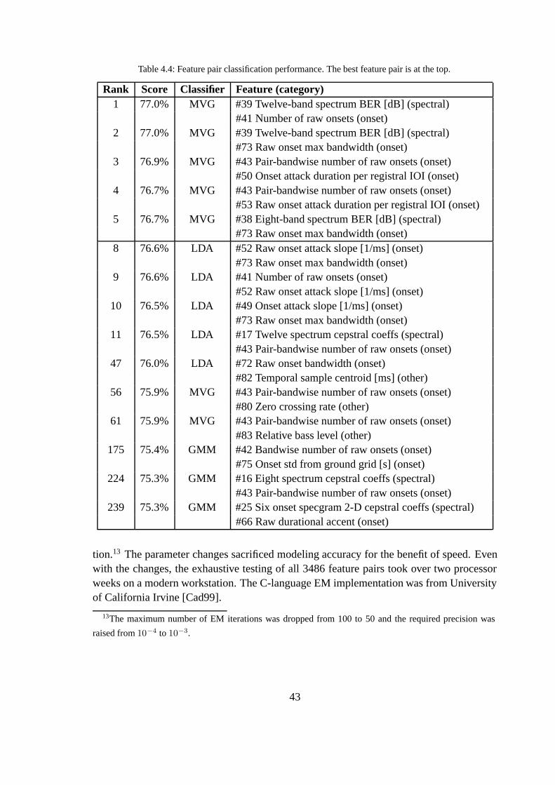
Table 4.4: Feature pair classification performance. The best feature pair is at the top.

Rank Score Classifier Feature (category)1 77.0% MVG #39 Twelve-band spectrum BER [dB] (spectral)

#41 Number of raw onsets (onset)2 77.0% MVG #39 Twelve-band spectrum BER [dB] (spectral)

#73 Raw onset max bandwidth (onset)3 76.9% MVG #43 Pair-bandwise number of raw onsets (onset)

#50 Onset attack duration per registral IOI (onset)4 76.7% MVG #43 Pair-bandwise number of raw onsets (onset)

#53 Raw onset attack duration per registral IOI (onset)5 76.7% MVG #38 Eight-band spectrum BER [dB] (spectral)

#73 Raw onset max bandwidth (onset)8 76.6% LDA #52 Raw onset attack slope [1/ms] (onset)

#73 Raw onset max bandwidth (onset)9 76.6% LDA #41 Number of raw onsets (onset)

#52 Raw onset attack slope [1/ms] (onset)10 76.5% LDA #49 Onset attack slope [1/ms] (onset)

#73 Raw onset max bandwidth (onset)11 76.5% LDA #17 Twelve spectrum cepstral coeffs (spectral)

#43 Pair-bandwise number of raw onsets (onset)47 76.0% LDA #72 Raw onset bandwidth (onset)

#82 Temporal sample centroid [ms] (other)56 75.9% MVG #43 Pair-bandwise number of raw onsets (onset)

#80 Zero crossing rate (other)61 75.9% MVG #43 Pair-bandwise number of raw onsets (onset)

#83 Relative bass level (other)175 75.4% GMM #42 Bandwise number of raw onsets (onset)

#75 Onset std from ground grid [s] (onset)224 75.3% GMM #16 Eight spectrum cepstral coeffs (spectral)

#43 Pair-bandwise number of raw onsets (onset)239 75.3% GMM #25 Six onset specgram 2-D cepstral coeffs (spectral)

#66 Raw durational accent (onset)

tion.13 The parameter changes sacrificed modeling accuracy for the benefit of speed. Evenwith the changes, the exhaustive testing of all 3486 feature pairs took over two processorweeks on a modern workstation. The C-language EM implementation was from Universityof California Irvine [Cad99].

13The maximum number of EM iterations was dropped from 100 to 50 and the required precision was

raised from 10−4 to 10−3.

43

Table 4.5: Best suboptimal feature subset obtained with random subset sequential backwards eliminationwith linear discriminant analysis (LDA). The performance score of LDA with these 16 features is 77.7%.

Number Name Category6 Onset energy ratio Spectral9 Onset spectrum bandwidth [mel] Spectral

17 Twelve spectrum cepstral coeffs Spectral23 Eight spectrum delta cepstral coeffs Spectral29 Eight-band onset spectrum BER Spectral31 Four-band onset spectrum BER [dB] Spectral38 Eight-band spectrum BER [dB] Spectral40 Number of onsets Onset41 Number of raw onsets Onset52 Raw onset attack slope [1/ms] Onset62 Raw registral IOI per tatum Onset63 Raw registral IOI deviation from tatum [ms] Onset64 Durational accent Onset66 Raw durational accent Onset71 Raw onset band centroid Onset72 Raw onset bandwidth Onset

The best feature subset obtained with random subset sequential backwards elimination us-ing LDA is listed in Table 4.5. The features are a mixture of features from both spectral andonset categories. The best discrimination score, 77.7%, is reached with the combination ofthese 16 features and using the LDA classifier. The improvement over the best feature pairis a tiny 0.7 percentage units. It may be speculated that significantly better performancecould be gained from using more than two features with a GMM classifier having highenough modeling accuracy, but finding that set of features would require significantly morecomputing power.

There clearly is overlap between the best feature pairs and the best suboptimal feature set inTable 4.5. Moreover, there is even overlap between the features in the suboptimal set: e.g.,the features #29 and #31 basically measure the same thing, only the number of bands andthe scale (linear vs. dB) is different. The fact that this is required for better discriminationperformance is evidence of LDA being a little too simple a statistical model for this use. Itis nevertheless fast, and consequently the phenomenal accent model uses the set of featureslisted in Table 4.5 and the LDA classifier.

4.3.4 Phenomenal accent model

As stated above, the aim of the phenomenal accent model is to produce a single normalizedvalue representing the total phenomenal accentuation (objective acoustic evidence of a beat)

44

at the given observation point. Therefore, the phenomenal accent model itself is a fairlycomplex decision function Ap(x) from N-dimensional feature vector domain D ⊂ R

N torange R ⊂ R that incorporates the specified statistical classifier.

An intuitive normalized measure of phenomenal accentuation is the posterior P (ωb|x), thatis, the probability of a beat ωb given the acoustic observation x. Furthermore, it is readilycomputed by the maximum a posteriori (MAP) classifier, and thus is easy to use. Accordingto the log-likelihood Bayes’ formula, Equation (3), the phenomenal accent equals

Ap(x) = P (ωb|x) = 1

exp [L(x, ωo)− L(x, ωb) + P(ωo)− P(ωb)] + 1, (27)

where the log-likelihoods L(x, ωi) and the log-priors P(ωi) are readily available for bothclasses ωi ∈ {ωb, ωo}. The probability of an offbeat P (ωo|x) is easy to compute from Ap

because the number of classes is fixed,

P (ωo|x) = 1− P (ωb|x) = 1− Ap(x). (28)

In short, the feature vector x is the input and the probabilities P (ωb|x) and P (ωo|x) are theoutputs of the phenomenal accent model.

4.4 Beat grid estimation

The next and final step in beat tracking after onset detection (Section 4.1) and tatum gridestimation (Section 4.2) is to determine the period ∆ ∈ {1, 2, . . . , ∆max} and phase φ ∈{1, 2, . . . , ∆} of the beat, given phenomenal accentuation (Section 4.3) as a functionof the metrical ground grid (Section 4.2). This is the process of finding which metricalground grid pulses are beats, essentially by filtering phenomenal accentuation data in orderto reveal periodicities.

A raw sequence of phenomenal accents Ap[n] only contains temporally uncorrelated infor-mation, whereas the most important aspect of beats is the temporal recurrence. We want tocompute the probability of a beat interpretation (∆, φ), given the sequence of observationsAp[n], according to Bayes’ formula14 (1),

P (∆, φ|Ap[n]) =P (Ap[n]|∆, φ)P (∆, φ)∑

i

∑j P (Ap[n]|∆i, φj)P (∆i, φj)

. (29)

Here P (Ap[n]|∆, φ) is the likelihood of observing the sequence of samples, assuming agiven beat interpretation, and P (∆, φ) is the prior probability of an interpretation.

14Again, the premiss for (29), requiring that (∆ i, φi) partition the certain eventS , holds.

45

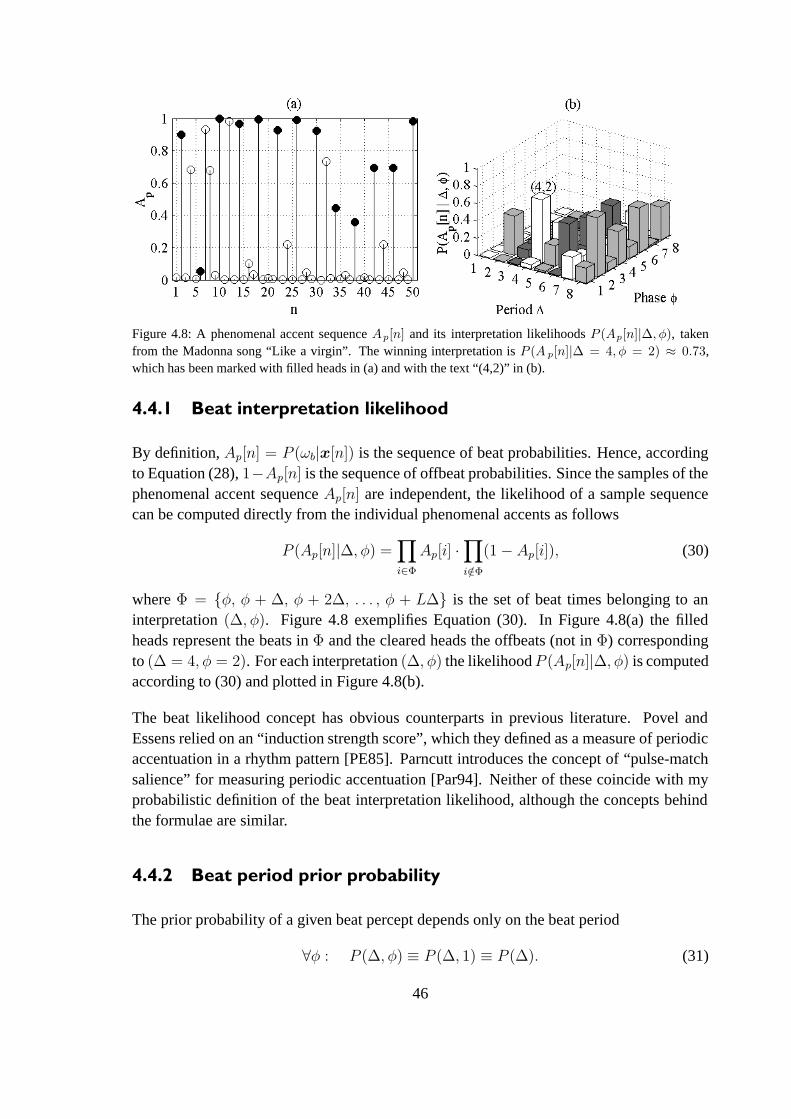
Figure 4.8: A phenomenal accent sequence Ap[n] and its interpretation likelihoods P (Ap[n]|∆, φ), takenfrom the Madonna song “Like a virgin”. The winning interpretation is P (A p[n]|∆ = 4, φ = 2) ≈ 0.73,which has been marked with filled heads in (a) and with the text “(4,2)” in (b).

4.4.1 Beat interpretation likelihood

By definition, Ap[n] = P (ωb|x[n]) is the sequence of beat probabilities. Hence, accordingto Equation (28), 1−Ap[n] is the sequence of offbeat probabilities. Since the samples of thephenomenal accent sequence Ap[n] are independent, the likelihood of a sample sequencecan be computed directly from the individual phenomenal accents as follows

P (Ap[n]|∆, φ) =∏i∈Φ

Ap[i] ·∏i/∈Φ

(1− Ap[i]), (30)

where Φ = {φ, φ + ∆, φ + 2∆, . . . , φ + L∆} is the set of beat times belonging to aninterpretation (∆, φ). Figure 4.8 exemplifies Equation (30). In Figure 4.8(a) the filledheads represent the beats in Φ and the cleared heads the offbeats (not in Φ) correspondingto (∆ = 4, φ = 2). For each interpretation (∆, φ) the likelihoodP (Ap[n]|∆, φ) is computedaccording to (30) and plotted in Figure 4.8(b).

The beat likelihood concept has obvious counterparts in previous literature. Povel andEssens relied on an “induction strength score”, which they defined as a measure of periodicaccentuation in a rhythm pattern [PE85]. Parncutt introduces the concept of “pulse-matchsalience” for measuring periodic accentuation [Par94]. Neither of these coincide with myprobabilistic definition of the beat interpretation likelihood, although the concepts behindthe formulae are similar.

4.4.2 Beat period prior probability

The prior probability of a given beat percept depends only on the beat period

∀φ : P (∆, φ) ≡ P (∆, 1) ≡ P (∆). (31)

46

Parncutt defines a lognormal probability distribution for the prior, which he calls the pulse-period salience function

P (∆) =1√2πσ

exp

[−12

(1

σlog10

∆q

µ

)2], (32)

in which the parameters µ = 600 ms, the 100 BPM moderate beat period, and σ = 0.02,the beat period deviation, are fixed constants [Par94], and q is the tatum period (see Sec-tion 4.2). Note that additional normalization by κ would be required to make the priors sumup to unity, ∑

i

∑j

P (∆i, φj) =∑i

κiP (∆i) = 1,

which would nevertheless be done in vain, because the factor κ would cancel out of Equa-tion (29) in the end.

4.4.3 Causal beat grid assignment

As stated in the beginning of Section 4, the whole proposed meter analysis algorithm op-erates causally, which obviously must hold for the beat grid estimation as well. Ultimatelythe beat period and phase are chosen in a similar process as the tatum period, using anexponentially decaying window for past data, implemented with a leaky integrator (seeSection 4.2).

One term of the likelihood product, Equation (30), is evaluated at each time instant n∗

for all beat interpretations (∆, φ). The term a(∆, φ) equals either Ap[n∗] or 1 − Ap[n

∗],respectively depending on whether the sample belongs to the interpretation’s set of beats Φor not. The likelihood product is then accumulated sample after sample

P (Ap[n], n ≤ n∗|∆, φ) = a(∆, φ)cf · P (Ap[n], n ≤ n∗ − 1|∆, φ)cl. (33)

The coefficients are cl = 2−1/10 and cf = 1−cl: the accumulated beat likelihood represents

the likelihood only in the range of about 10 samples (approximately 10 · 120 ms = 1.2 s) tothe past.

The posterior (29) is computed for all beat interpretations from the priors (32) and likeli-hoods (33). The beat period ∆ is simply the period with the maximum posterior probability,ignoring the phase,

∆[n∗] = argmax∆

P (∆, φ|Ap[n], n ≤ n∗), (34)

yielding a beat period ∆[n∗] · q in absolute temporal units. Then, the winning beat phase φ

is simply chosen maximum a posteriori,

φ[n∗] = argmaxφ

P (∆[n∗], φ|Ap[n], n ≤ n∗). (35)

47

Having chosen the beat period ∆ and phase φ, the grid points n satisfying

n− φ = 0 (mod ∆) (36)

are found as the beat grid.

4.5 Estimation of subordinate metrical levels

Handed with knowledge of the tatum period q and the number of tatums per beat ∆, it is rel-atively trivial to fill in the pulses on the subordinate metrical levels between tatum and beat.The metrical well-formedness rule #3 of Lerdahl and Jackendoff states that the pulse peri-ods of neighboring metrical levels are always related by a duple or a triple division [LJ83,p. 69].

Most often there are not more than 6 tatums/beat, meaning that there are at most two sub-ordinate metrical levels between the tatum and the beat. More specifically, ∆ is iterativelydivided by 2 and by 3 to observe if there is a duple or a triple relation to the next-lowermetrical pulse period. If there is no remainder from the division, a metrical level with abeat period half or a third the beat period and phase coinciding with the beat phase is as-sumed. The division result is further divided by 2 and 3 to search for a second subordinatelevel. In the case of both a duple and a triple relation the ambiguity of the order of thelevels remains unanswered, and the algorithm currently simply chooses the resolution withthe triple division on the level next to the tatum.

48

5 Model performance

The proposed meter recognition model consists of four main components, sound onset de-tection, tatum grid estimation, phenomenal accent model, and beat grid estimation, as de-scribed in Section 4. All of these components have an influence on the performance of theoverall model, and therefore it is reasonable to assess each of the components separately, inaddition to evaluating the performance of the overall system.

Furthermore, in order to assess the contribution of the individual components to total per-formance, we would ideally like to evaluate the components and the total system with thesame metric. The metric used is a beat tracker performance metric. Evaluating the effi-ciency of an onset detector with a beat tracker metric in general is not very informative,but in this setting it provides an insight of the effect of the onset detector in terms of beattracking performance. Moreover, it is not possible to evaluate onset detector efficiency assuch unless the source material is extensively labeled by hand.

In addition to analyzing the proposed model, the comparison of it with previously pub-lished models provides useful information about the model in general. The proposed modelis compared to the model of Scheirer due to the similar setting of the models; they areboth causal and are capable of processing real-world musical signals [Sch98b]. In fact,no other model among the reviewed ones possess these characteristics. For simulations,I used Scheirer’s own implementation of his model, which is freely available for researchpurposes, with the author’s parameter settings intact [Sch98a].

Beat tracking performance was computed by measuring the distance from a computed beatgrid to the annotated beat grid. For each of the 330 songs in the corpus, the ground truthbeat was annotated as described in Appendix A. Various statistics of the music corpus aredescribed in Appendix A and Section 4.3.

5.1 Performance measure

Goto and Muraoka have considered performance evaluation of beat tracking systems. Theyhave published guidelines on what to take into account of the beat tracking result and howto measure each deviation from the ground truth. The performance is the expressed as amultidimensional vector that incorporates the different aspects of errors. [GM97]

More recently, also Cemgil and his colleagues have set out to devise a beat tracking per-formance metric [CKDH01]. Because the measure they give is a scalar and thus facilitatestrivial comparison of the performance of two or more beat trackers, I will use their measurehere.

49

Figure 5.1: (a) Percentage of beats and offbeats recognized correctly using the proposed model (solid line) andusing only phenomenal accent modeling (dashed line). (b) Performance ρ of the whole model (solid line) andthe phenomenal accent model (dashed line). Highest obtainable performance after onset detection (dash-dot)and tatum estimation (dotted line) are also shown.

Given an I-length vector ψ of correct beat times and a J-length vector t of estimated beattimes, in seconds, Cemgil et al. define the tempo tracking performance measure

ρ(ψ, t) =

∑imaxj W (ψi − tj)

(I + J)/2· 100%, (37)

W (d) = exp[−d2/(2σ2

e)],

where σe = 40 ms is a parameter controlling the spread of the Gaussian observation win-dow W (d). “The tracking index ρ can be roughly interpreted as percentage of ‘correct’beats”, as Cemgil et al. put it. A value of ρ = 100% equates to ψ and t being identi-cal. [CKDH01]

5.2 Results

Figure 5.1 shows a breakdown of the performance of different components of the pro-posed algorithm. In Figure 5.1(a) the performance of the whole system is compared to theperformance of the phenomenal accent model, i.e., the system with beat grid estimationturned off. The ordinate corresponds to the percentage of correct classifications, given themetrical ground grid, while the abscissa designates song rank. The solid line reports correctclassification percentage when temporal periodicity is used (whole system) and the dashedline when it is not used (system without beat grid estimation). It can be seen that in generalthe temporal periodicity does help in the classification somewhat, but that it becomes reallyuseful only when the underlying phenomenal accentuation information is reliable enough.In the whole corpus 80.3% of grid points are classified correctly based on phenomenal ac-centuation purely (using the LDA classifier with features from Table 4.5) and 82.7% arerecognized correctly in beat grid estimation.

50

Figure 5.2: Performance ρ of the proposed model (solid line) and the Scheirer model (dash-dot line).

Figure 5.1(b) provides a view of the contribution of each of the four main components to theoverall performance. First, the dash-dotted line illustrates the absolute highest performancescore obtainable by representing the beat tracker output with the onsets nearest to annotatedbeats. Thus, it is a measure of the onset detector performance. This is also a test of theassumption that beats usually coincide with onsets.

Next, the dotted line in Figure 5.1(b) follows the highest performance score obtainable byconsidering the ground-level grid points nearest to annotated beats, i.e., it is a measure orthe joint performance of the onset detector and the tatum grid estimator. The fact that thetatum grid performance (dotted line) surpasses the onset detector performance (dash-dottedline) reflects the fact that the tatums coincide with beats more often than the onsets do. Thisstems directly from the fact that beats are tatums, i.e., higher-level pulses are also pulses onlower levels.

The dashed line in Figure 5.1(b) shows the joint performance of the onset detector, tatumgrid estimator and phenomenal accent model. The line corresponds to actual classifica-tion results of the statistical phenomenal accent model using LDA and the features fromTable 4.5. Clearly, there is some room for improvement.

Finally, the solid line in Figure 5.1(b) summarizes the performance of the whole proposedmeter recognition model. The figure tells that the fourth component, beat grid estimation,does have a positive effect on performance in the region where the underlying componentswork sufficiently well. If the phenomenal accent model does not give good enough esti-mates, then the beat grid estimator cannot rescue performance.

Figure 5.2 shows a comparison of the performance of the proposed model and Scheirer’smodel [Sch98b]. In this simulation it appeared that Scheirer’s model provides better per-formance for all test samples. The performance of the proposed model comes nearest toScheirer’s in the easiest and the hardest cases.

51

To summarize the average performance over all songs in the corpus, the collective perfor-mance measure is defined:

ρ({ψ}, {t}) =∑

k

∑imaxj W (ψk,i − tk,j)∑

k(Ik + Jk)/2· 100%, (38)

where {ψ} is a set of Ik-length correct beat time vectors and {t} is a set of Jk-lengthestimated beat time vectors corresponding to song k.

Now the collective beat tracking performances are ρ = 40% for the proposed model andρ = 51% for the Scheirer model. Based on the tatum grid of the proposed model, thehighest obtainable performance score would be 78%. This shows that the tatum grid is afeasible starting point for beat induction.

Published results of noncausal beat trackers operating on MIDI input routinely report per-formance values ρ of 90% or more [CKDH01] [Dix01b]. Nevertheless, the two differences(causal vs. noncausal and acoustic signal vs. MIDI input) really make a difference to theperformance. Leveraging the results from MIDI beat trackers for the benefit of audio signalbeat tracking requires an amount of preprocessing that resembles an automatic transcriber.

52

6 Conclusions

The problem of musical meter recognition is a relevant research topic for the music analy-sis and musical signal processing communities. We have witnessed an explosion of modelsattempting meter recognition or beat tracking, which is a special case of meter analysis.In this work I reviewed 21 previously published models, of which eight have been pub-lished this year (2001). The reviewed models are all different, each having a specific setof assumptions about the analysis problem. I have analyzed the models based on causality,applicability for acoustic input, and functional similarity.

This thesis describes a novel computational model for the recognition of musical meterfrom an acoustic signal of music. The proposed model comprises four main components:the onset detector, the tatum grid estimator, the phenomenal accent model, and the beatgrid estimator. The model construction is a mixture of signal processing, music theory, andstatistical pattern recognition.

The onset detector computes amplitude envelopes from the input signal. Amplitude en-velopes are computed for multiple frequency bands for robustness. Onset events are trig-gered by rapid increases in the amplitude envelopes. Further characteristics of onsets arecomputed, including onset amplitudes, bandwise inter-onset intervals, and sound attacktimes.

The tatum grid estimator processes the stream of onsets and looks for the tatum, an intrinsicquantization unit, in inter-onset intervals. The tatum grid is estimated in causal fashion,updating an internal histogram as new onsets are detected. Finally, a derivate of the tatumcalled metrical ground grid is fabricated. The ground is a variant of the tatum where alldiscontinuities in period have been removed.

The proposed meter recognizer includes an internal model of phenomenal accent. In build-ing this submodel, the performance of 83 acoustic signal features was evaluated, and a finalset of 16 features was selected. The accent model is built from acoustic signal featureswith linear discriminant analysis (LDA). The phenomenal accent is modeled as a posteriorprobability, as computed by LDA.

The beat grid estimator combines results from onset detection, tatum estimation, and phe-nomenal accent modeling. It comprises simple probability calculations for finding the mostprobable periodicity from phenomenal accent data. After knowing the beat, it is used incombination with the tatum to compute pulses on subordinate metrical levels between thebeat and tatum.

The proposed system aims at generality in regard to musical genres. The music corpusused for building the model and verifying its performance comprises excerpts from blues,

53

classical, dance, folk, funk, jazz, pop, R&B, rap, rock, soul, and world music. The corpusconsists of 330 monophonic excerpts of music, each of about one minute in duration. Inaddition to the acoustic signals, the corpus contained manually annotated beat positions asa metrical reference. Beat annotation was done, because it is the most intuitive metricalcomponent to annotate in a real-time listening test.

The proposed method consumes acoustic input and operates causally. These two qualitiesimpose quite strict restrictions on model design, and only two of the 21 reviewed modelsqualified as comparable to the proposed model in this respect. Fortunately, Eric Scheirer,the author of one of these two models, provided a reference implementation of his model.This allowed me to compare the performances of the proposed model and his model in beattracking. It turned out that Scheirer’s model outperformed the proposed model for all of the330 pieces of music used for testing, but that the performance difference was small for theeasiest and the hardest pieces. However, Scheirer’s model can only be used for finding thebeat, it does not find other metrical levels.

In the course of this work I learned that tatum estimation works more robustly if onlyonset timing is used and further information on sound quality, such as loudness, timbre, orpitch, is discarded. On the other hand, estimation of the beat relies on these descriptors.The features used for phenomenal accent estimation comprise signal spectrum features aswell as features derived from onset data. Conservative signal descriptors such as the zerocrossing rate or the crest factor did not have much use here.

The availability of beats and tatums makes it feasible to automatically measure musicaltime from a piece of music and to compare different pieces on a musical time scale. Thisenables applications which compute and handle metrical intervals between musical eventsin addition to computing absolute time intervals. The meter model can be used as is in amusical signal editing application to allow for automatization of time-related operations.Knowledge of the beat and the tatum also facilitates automatic matching of two musicalpieces, even if the pieces have different tempi and tatums. Robust meter recognition is avital component of music information retrieval applications.

The meter model can only recognize metrical levels from the beat downwards. Furtherresearch is required in order to find the measure from an acoustic signal. The harmonicstructure of music has to be exploited in addition to the phenomenal cues presented in thiswork. Apart from the measure, the current model attempts to recognize the metrical levelsthat span the musical time base. The distribution of onsets and accents in this time baseshould be further investigated to recognize the fine structure of rhythm. The deliberatedeviation from the metrical grid is a well known method of musical expression, and thedeviations also carry information relevant to the listener. An example of deliberate deviationfrom metrical grid is swing, very often used in jazz and funk music.

54

One weakness of the proposed model is the cumulation of errors in the processing chain.The performance evaluation showed that the beat estimator does not have any chance ofworking if the phenomenal accent model is not working properly. Furthermore, if the tatumis not reliable, the beat will not be found; if the detected onsets do not carry enough in-formation, the correct tatum cannot be estimated. The robustness of the model should beimproved, and one way to do this would be to make e.g. tatum and beat estimation worktogether instead of working separately.

The tatum estimator algorithm has been published in [Sep01]. A second publication on thephenomenal accent model is currently under preparation. A real-time implementation ofthe tatum estimator may be downloaded from [SM00].

55

References

[AD90] Paul E. Allen and Roger B. Dannenberg. Tracking musical beats in realtime. In Proc. Int. Comp. Music Conf. (ICMC), pages 140–143, Glasgow,Scotland, 1990.

[AN97] Jont B. Allen and Stephen T. Neely. Modeling the relation between the in-tensity just-noticeable difference and loudness for pure tones and widebandnoise. J. Acoust. Soc. Am., 102(6):3628–3646, 1997.

[BC94] Guy J. Brown and Martin P. Cooke. Computational auditory scene analysis.Computer Speech and Lang., 8(4):297–336, 1994.

[Bil93a] Jeff A. Bilmes. Techniques to foster drum machine expressivity. In Proc.Int. Comp. Music Conf. (ICMC), pages 276–283, Tokyo, Japan, 1993.

[Bil93b] Jeffrey A. Bilmes. Timing is of the essence: Perceptual and computationaltechniques for representing, learning, and reproducing expressive timing inpercussive rhythm. M.Sc. thesis, Massachusetts Institute of Tech., Septem-ber 1993.

[BKWW99] Thomas L. Blum, Douglas F. Keislar, James A. Wheaton, and Erling H.Wold. Method and article of manufacture for content-based analysis,storage, retrieval, and segmentation of audio information. U.S. Patent#5,918,223, 1999.

[Bro93] Judith C. Brown. Determination of the meter of musical scores by autocor-relation. J. Acoust. Soc. Am., 94(4):1953–1957, 1993.

[Cad99] Igor Cadez. DataLab gaussian mixture modeling software. http://www.datalab.uci.edu/software.html, August 1999.

[Car01] Peter Cariani. Temporal codes, timing nets and music perception. J. NewMusic Research, 30(2), 2001. (to appear).

[CJK+85] C. Chafe, D. Jaffe, K. Kashima, B. Mont-Reynaud, and J. Smith. Sourceseparation and note identification in polyphonic music. Report STAN-M-29, Stanford Univ., 1985.

[CK99] Edward C. Carterette and Roger A. Kendall. Comparative music perceptionand cognition. In D. Deutsch, editor, The Psychology of Music, pages 725–791. Academic Press, San Diego, CA, USA, 2nd edition, 1999.

[CKDH01] Ali Taylan Cemgil, Bert Kappen, Peter Desain, and Henkjan Honing. Ontempo tracking: Tempogram representation and kalman filtering. J. NewMusic Research, 2001. (to appear).

56

[Cla99] Eric F. Clarke. Rhythm and timing in music. In D. Deutsch, editor, ThePsychology of Music, pages 473–500. Academic Press, San Diego, CA,USA, 2nd edition, 1999.

[DH73] Richard O. Duda and Peter E. Hart. Pattern Classification and Scene Anal-ysis. John Wiley & Sons, 1973.

[DH93] Peter Desain and Henkjan Honing. Time in contemporary musical thought:Tempo curves considered harmful. Contemporary Music Review, 7(2):123–138, 1993.

[Dix01a] Simon Dixon. Automatic extraction of tempo and beat from expressiveperformances. J. New Music Research, 30(1), 2001. (to appear).

[Dix01b] Simon Dixon. An empirical comparison of tempo trackers. In 8th BrazilianSymposium on Computer Music, Fortaleza, Brazil, 2001.

[Eck01] Douglas Eck. A network of relaxation oscillators that finds downbeats inrhythms. Tech. report IDSIA-06-01, IDSIA, Lugano, Switzerland, 2001.

[EGP00] Douglas Eck, Michael Gasser, and Robert Port. Dynamics and embodimentin beat induction. In Rhythm Perception and Production, pages 157–170.Swets & Zeitlinger, Lisse, The Netherlands, 2000.

[EK00] Antti Eronen and Anssi Klapuri. Musical instrument recognition using cep-stral coefficients and temporal features. In Proc. IEEE Int. Conf. Acoust.,Speech, and Signal Proc. (ICASSP), volume 2, pages 753–756, Istanbul,Turkey, 2000.

[Foo97] Jonathan T. Foote. Content-based retrieval of music and audio. In C.-C.Jay Kuo et al., editor, Multimedia Storage and Archiving Systems II, Proc.of SPIE, volume 3229, pages 138–147, 1997.

[Fou01] Sonic Foundry. Acid pro 3 software. http://www.sonicfoundry.com, 2001.

[FU01] Jonathan Foote and Shingo Uchihashi. The beat spectrum: A new approachto rhythm analysis. In Proc. IEEE Int. Conf. on Multimedia and Expo,Tokyo, Japan, 2001.

[GH96] Zoubin Ghahramani and Geoffrey E. Hinton. Parameter estimation for lin-ear dynamical systems. Tech. report CRG-TR-96-2, Univ. of Toronto,Toronto, Canada, 1996.

[GM97] Masataka Goto and Yoichi Muraoka. Issues in evaluating beat trackingsystems, 1997.

[GM98] Masataka Goto and Yoichi Muraoka. Music understanding at the beat level:Real-time beat tracking for audio signals. In D.F. Rosenthal and H.G.

57

Okuno, editors, Computational Auditory Scene Analysis, pages 157–176.Lawrence Erlbaum Associates, Mahwah, NJ, USA, 1998.

[GPD00] Fabien Gouyon, François Pachet, and Olivier Delerue. On the use of zero-crossing rate for an application of classification of percussive sounds. InProc. COST G-6 Conf. on Digital Audio Effects (DAFX), Verona, Italy,2000.

[GR99] Zoubin Ghahramani and Sam Roweis. Probabilistic models for unsuper-vised learning. Neural Information Processing Systems (NIPS) Tutorial,December 1999.

[Ins01] Native Instruments. Traktor software. http://www.native-instruments.de,2001.

[Kar99] Matti Karjalainen. Kommunikaatioakustiikka (esipainos). Teknillinen Ko-rkeakoulu, Espoo, Finland, 1999.

[Kay93] Steven M. Kay. Fundamentals of Statistical Signal Processing: EstimationTheory. Prentice Hall Int., Englewood Cliffs, NJ, USA, 1993.

[Kla98] Anssi Klapuri. Automatic transcription of music. M.Sc. thesis, TampereUniv. of Tech., Tampere, Finland, 1998.

[Kla99] Anssi Klapuri. Sound onset detection by applying psychoacoustic knowl-edge. In Proc. IEEE Int. Conf. Acoust., Speech, and Signal Proc. (ICASSP),volume 6, pages 3089–3092, 1999.

[Lar01] Jean Laroche. Estimating tempo, swing and beat locations in audio record-ings. In Proc. IEEE Workshop on Applicat. of Signal Proc. to Audio andAcoust. (WASPAA), pages 135–138, New Paltz, NY, USA, October 2001.

[Lee91] Cristopher S. Lee. The perception of metrical structure: Experimental ev-idence and a model. In P. Howell, R. West, and I. Cross, editors, Repre-senting Musical Structure, pages 59–127. Academic Press, London, UnitedKingdom, 1991.

[Li00] Stan Z. Li. Content-based classification and retrieval of audio usingthe nearest feature line method. IEEE Trans. Speech and Audio Proc.,8(5):619–625, 2000.

[LJ83] Fred Lerdahl and Ray Jackendoff. A Generative Theory of Tonal Music.MIT Press, Cambridge, MA, USA, 1983.

[LK94] Edward W. Large and John F. Kolen. Resonance and the perception ofmusical meter. Connection Science, 6(2/3):177–208, 1994.

58

[LM98] Huan Liu and Hiroshi Motoda. Feature Selection for Knowledge Discoveryand Data Mining. Kluwer Academic, Norwell, MA, USA, 1998.

[MZ94] Guerino Mazzola and Oliver Zahorka. Tempo curves revisited: Hierarchiesof performance fields. Comp. Music J., 18(1):40–52, 1994.

[OS89] Alan V. Oppenheim and Ronald W. Schafer. Discrete-time Signal Process-ing. Prentice Hall, Englewood Cliffs, NJ, USA, 1989.

[Pal99] Carlos Palombini. Musique concrète revisited. In L. Sitsky, editor, TheTwentieth-century Music Avant-garde. Greenwood Publishing Group, Inc.,Westport, CT, USA, 1999.

[Pap91] Athanasios Papoulis. Probability, Random Variables, and Stochastic Pro-cesses. McGraw-Hill, 3rd edition, 1991.

[Par94] Richard Parncutt. A perceptual model of pulse salience and metrical accentin musical rhythms. Music Perception, 11(4):409–464, 1994.

[PC95] Cristopher J. Plack and Robert P. Carlyon. Loudness perception and inten-sity coding. In B.C.J. Moore, editor, Hearing, Handbook of Perception andCognition. Academic Press, San Diego, CA, USA, 2nd edition, 1995.

[PE85] Dirk-Jan Povel and Peter Essens. Perception of temporal patterns. MusicPerception, 2(4):411–440, 1985.

[PMH00] Geoffroy Peeters, Stephen McAdams, and Perfecto Herrera. Instrumentsound description in the context of MPEG-7. In Proc. Int. Comp. MusicConf. (ICMC), Berlin, Germany, 2000.

[Rap01] Cristopher Raphael. Automated rhythm transcription. In Proc. Int. Sympo-sium on Music Inform. Retriev. (ISMIR), pages 99–107, Bloomington, IN,USA, October 2001.

[RJ93] Lawrence Rabiner and Biing-Hwang Juang. Fundamantals of SpeechRecognition. Prentice Hall, 1993.

[Ros92] David F. Rosenthal. Machine Rhythm: Computer Emulation of HumanRhythm Perception. Ph.D. thesis, Massachusetts Institute of Tech., August1992.

[Sch85] W. Andrew Schloss. On the Automatic Transcription of Percussive Music— From Acoustic Signal to High-level Analysis. Ph.D. thesis, CCRMA,Stanford Univ., May 1985.

[Sch95] Eric D. Scheirer. Extracting expressive performance information fromrecorded music. M.Sc. thesis, Massachusetts Institute of Tech., Septem-ber 1995.

59

[Sch98a] Eric D. Scheirer. tapping software. http://sound.media.mit.edu/∼eds/beat/tapping.tar.gz, 1998.

[Sch98b] Eric D. Scheirer. Tempo and beat analysis of acoustic musical signals. J.Acoust. Soc. Am., 103(1):588–601, January 1998.

[Sch00] Eric D. Scheirer. Music-listening Systems. Ph.D. thesis, MassachusettsInstitute of Tech., June 2000.

[Sep01] Jarno Seppänen. Tatum grid analysis of musical signals. In Proc. IEEEWorkshop on Applicat. of Signal Proc. to Audio and Acoust. (WASPAA),pages 131–134, New Paltz, NY, USA, October 2001.

[Sla93] Malcolm Slaney. An efficient implementation of the Patterson–Holdsworthauditory filter bank. Apple computer tech. report #35, Apple Computer,Inc., 1993.

[SM00] Jarno Seppänen and Piotr Majdak. rhythm_estimator software.ftp://iem.kug.ac.at/pd/Externals/RHYTHM/, June 2000.

[Smi96] Leslie S. Smith. Onset-based sound segmentation. In D.S. Touretzky,M.C. Mozer, and M.E. Haselmo, editors, Advances in Neural InformationProcessing Systems, volume 8, pages 729–735. MIT Press, 1996.

[Smi99] Leigh M. Smith. A Multiresolution Time-frequency Analysis and Interpre-tation of Musical Rhythm. Ph.D. thesis, Univ. of Western Australia, July1999.

[SS97] Eric Scheirer and Malcolm Slaney. Construction and evaluation of a robustmultifeature speech/music discriminator. In Proc. IEEE Int. Conf. Acoust.,Speech, and Signal Proc. (ICASSP), volume 2, pages 1331–1334, Munich,Germany, April 1997.

[SS01] William A. Sethares and Thomas W. Staley. Meter and periodicity in musi-cal performance. J. New Music Research, 2001. (to appear).

[Sys99] E-mu Systems. Emulator ultra 4 sampler hardware. http://www.emu.com,1999.

[TEC01] George Tzanetakis, Georg Essl, and Perry Cook. Automatic musical genreclassification of audio signals. In Proc. Int. Symposium on Music Inform.Retriev. (ISMIR), pages 205–210, Bloomington, IN, USA, October 2001.

[TG74] Julius T. Tou and Rafael C. Gonzales. Pattern Recognition Principles.Addison–Wesley, Reading, MA, USA, 1974.

[Tod94] Neil P. McAngus Todd. The auditory “primal sketch”: A multiscale modelof rhythmic grouping. J. New Music Research, 23(1):25–70, 1994.

60

[Toi97] Petri Toiviainen. Modelling the perception of metre with competing subhar-monic oscillators. In A. Gabrielsson, editor, Proc. 3rd Triennial ESCOMConf., pages 511–516, Uppsala, Sweden, 1997.

[Toi98] Petri Toiviainen. An interactive MIDI accompanist. Comp. Music J.,22(4):63–75, 1998.

[TS99] David Temperley and Daniel Sleator. Modeling meter and harmony: Apreference-rule approach. Comp. Music J., 23(1):10–27, 1999.

[Wal91] Gregory K. Wallace. The JPEG still picture compression standard. Comm.ACM, 34(4):30–44, 1991.

[WBKW96] Erling Wold, Thom Blum, Douglas Keislar, and James Wheaton. Content-based classification, search and retrieval of audio. IEEE Multimedia,3(3):27–36, 1996.

[ZF90] E. Zwicker and H. Fastl. Psychoacoustics — Facts and Models. Springer,Heidelberg, Germany, 1990.

[ZK99] Tong Zhang and C.-C. Jay Kuo. Hierarchical classification of audio datafor archiving and retrieving. In Proc. IEEE Int. Conf. Acoust., Speech, andSignal Proc. (ICASSP), volume 6, pages 3001–3004, Phoenix, AZ, USA,March 1999.

61

A Music corpus

The corpus collected in this work contains 330 musical signal excerpts, taken from commer-cial CD’s, at 44100 Hz sample rate. From each selected recording, a characteristic excerptwas extracted, which was then converted to a monophonic signal. The corpus contains18963 seconds (over 5 hours and 16 minutes) of music in total, whereby average excerptduration equals 57.5 seconds.

The musical excerpts were selected to contain a wide range of instruments, dynamic rangesand tempi. Recordings both with and without percussion, with and without vocals andof studio and live performances were included. Another goal was to include representativeexcerpts from different musical genres, ranging from jazz and rock through classical and bigband music to pop and electronic music. Excerpts of music recorded on different decadesis included. Figure A.1 shows a histogram of the original recording years of the songs; theyrange from the 1920’s to the year 2000.

The music material has an unambiguous meter present, although a part of the songs containsrubatos, ritardandos and accelerandos. The beat in each of the excerpts was carefully manu-ally annotated in real time by tapping along with a pen while the excerpt was being played.In real time listening, annotating the beat is the most natural task, while annotating someother (especially lower) metrical level, such as the tatum, is practically impossible. Thesound of the tapping of the pen on a table was recorded and the recordings were searchedfor transients. The annotated inter-beat intervals were plotted on screen and visually veri-fied.

Figure A.2 shows a more precise picture of the distribution of tempi in the corpus, computedfrom the intervals between annotated beat positions. The histograms verify the conjecturethat the beat is most salient in the vicinity of moderate tempo of about 100 BPM [Par94].

Figure A.1: Histogram (N=330) of song recording years.

62

Figure A.2: Corrected histograms (N=33156) of inter-beat intervals (IBI) in (a) period and (b) frequencyunits. The contributions of the seven genres are shown individually. The genres are numbered according toTable 4.2 on page 37.

The tempo histograms in Figure A.2 have been corrected to remove period-dependent dis-tortion caused by limited song duration. Put simply, the frequency of beats at e.g. 200 msperiod needs to be corrected by a factor of two compared with the frequency of 100 msbeats, because there are twice as many 100 ms beats than 200 ms beats in any excerptof music. Therefore, the frequency of beats F(p) at period p is corrected according toF(p) = F(p) · p to yield corrected frequency F(p).

Table A.1 below lists the names of the artists and songs in the music corpus in detail. Foreach excerpt, also the annotated genre and recording year are shown. The genre numberingis according to Table 4.2. Section 4.3 also shows statistics of the data in the corpus.

Table A.1: Music corpus samples.

Artist: Song, Genre number, Recording year Artist: Song, Genre number, Recording year–: Deck the halls, 1, 1994 666: Bomba, 2, 1999London concert orchestra: Swanlake: Hungariandance - Czardas, 1, –

Abba: Lay all your love on me, 5, –

Abba: S.O.S, 5, 1975 Abba: Waterloo, 5, 1974Abraham Laboriel: Dear friends, 4, 1993 Abraham Laboriel: Look at me, 4, 1993Academy chamber ensemble: Sonata in A-dur op.5/1:allegro, 1, 1983

Academy chamber ensemble: Sonata in A-dur op.5/1:andante–adagio, 1, 1983

Academy chamber ensemble: Sonata in A-dur op.5/1:gavotte (allegro), 1, 1983

Academy chamber ensemble: Sonata in A-dur op.5/1:larghetto–allegro, 1, 1983

Academy chamber ensemble: Sonata in e minor: al-legro, 1, 1983

Academy chamber ensemble: Sonata in e minor:allemande (andante allegro), 1, 1983

Academy chamber ensemble: Sonata in e minor: an-dante larghetto–adagio, 1, 1983

Academy chamber ensemble: Sonata in e minor:gavotte (allegro), 1, 1983

Academy chamber ensemble: Sonata in e minor: ron-deau, 1, 1983

Academy chamber ensemble: Sonata in e minor:sarabande (largo assai), 1, 1983

Ahmad Jamal: Autumn in New York, 4, 1958 Ahmad Jamal: The girl next door, 4, 1958Al DiMeola: Dark eye tango, 4, 1978 Al DiMeola: Mediterranean sundance, 4, 1977Alex Welsh: Maple leaf rag, 4, 1988 All-4-One: I turn to you, 6, 1996

63

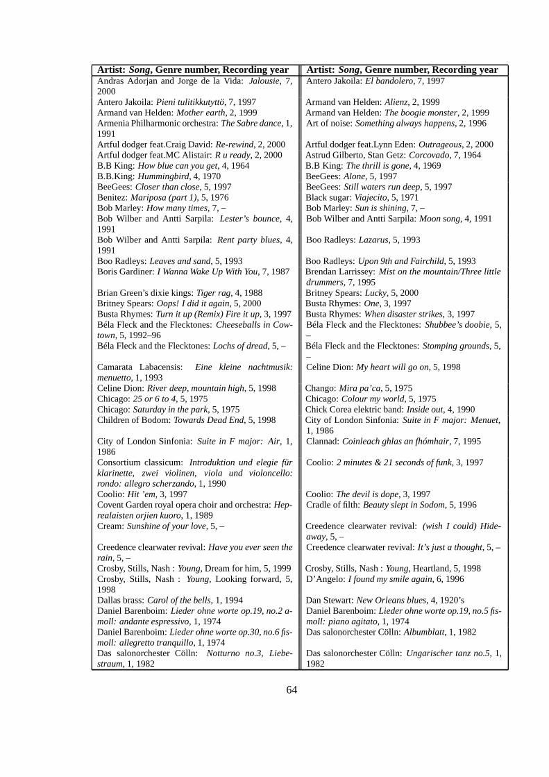
Artist: Song, Genre number, Recording year Artist: Song, Genre number, Recording yearAndras Adorjan and Jorge de la Vida: Jalousie, 7,2000

Antero Jakoila: El bandolero, 7, 1997

Antero Jakoila: Pieni tulitikkutyttö, 7, 1997 Armand van Helden: Alienz, 2, 1999Armand van Helden: Mother earth, 2, 1999 Armand van Helden: The boogie monster, 2, 1999Armenia Philharmonic orchestra: The Sabre dance, 1,1991

Art of noise: Something always happens, 2, 1996

Artful dodger feat.Craig David: Re-rewind, 2, 2000 Artful dodger feat.Lynn Eden: Outrageous, 2, 2000Artful dodger feat.MC Alistair: R u ready, 2, 2000 Astrud Gilberto, Stan Getz: Corcovado, 7, 1964B.B King: How blue can you get, 4, 1964 B.B King: The thrill is gone, 4, 1969B.B.King: Hummingbird, 4, 1970 BeeGees: Alone, 5, 1997BeeGees: Closer than close, 5, 1997 BeeGees: Still waters run deep, 5, 1997Benitez: Mariposa (part 1), 5, 1976 Black sugar: Viajecito, 5, 1971Bob Marley: How many times, 7, – Bob Marley: Sun is shining, 7, –Bob Wilber and Antti Sarpila: Lester’s bounce, 4,1991

Bob Wilber and Antti Sarpila: Moon song, 4, 1991

Bob Wilber and Antti Sarpila: Rent party blues, 4,1991

Boo Radleys: Lazarus, 5, 1993

Boo Radleys: Leaves and sand, 5, 1993 Boo Radleys: Upon 9th and Fairchild, 5, 1993Boris Gardiner: I Wanna Wake Up With You, 7, 1987 Brendan Larrissey: Mist on the mountain/Three little

drummers, 7, 1995Brian Green’s dixie kings: Tiger rag, 4, 1988 Britney Spears: Lucky, 5, 2000Britney Spears: Oops! I did it again, 5, 2000 Busta Rhymes: One, 3, 1997Busta Rhymes: Turn it up (Remix) Fire it up, 3, 1997 Busta Rhymes: When disaster strikes, 3, 1997Béla Fleck and the Flecktones: Cheeseballs in Cow-town, 5, 1992–96

Béla Fleck and the Flecktones: Shubbee’s doobie, 5,–

Béla Fleck and the Flecktones: Lochs of dread, 5, – Béla Fleck and the Flecktones: Stomping grounds, 5,–

Camarata Labacensis: Eine kleine nachtmusik:menuetto, 1, 1993

Celine Dion: My heart will go on, 5, 1998

Celine Dion: River deep, mountain high, 5, 1998 Chango: Mira pa’ca, 5, 1975Chicago: 25 or 6 to 4, 5, 1975 Chicago: Colour my world, 5, 1975Chicago: Saturday in the park, 5, 1975 Chick Corea elektric band: Inside out, 4, 1990Children of Bodom: Towards Dead End, 5, 1998 City of London Sinfonia: Suite in F major: Menuet,

1, 1986City of London Sinfonia: Suite in F major: Air, 1,1986

Clannad: Coinleach ghlas an fhómhair, 7, 1995

Consortium classicum: Introduktion und elegie fürklarinette, zwei violinen, viola und violoncello:rondo: allegro scherzando, 1, 1990

Coolio: 2 minutes & 21 seconds of funk, 3, 1997

Coolio: Hit ’em, 3, 1997 Coolio: The devil is dope, 3, 1997Covent Garden royal opera choir and orchestra: Hep-realaisten orjien kuoro, 1, 1989

Cradle of filth: Beauty slept in Sodom, 5, 1996

Cream: Sunshine of your love, 5, – Creedence clearwater revival: (wish I could) Hide-away, 5, –

Creedence clearwater revival: Have you ever seen therain, 5, –

Creedence clearwater revival: It’s just a thought, 5, –

Crosby, Stills, Nash : Young, Dream for him, 5, 1999 Crosby, Stills, Nash : Young, Heartland, 5, 1998Crosby, Stills, Nash : Young, Looking forward, 5,1998

D’Angelo: I found my smile again, 6, 1996

Dallas brass: Carol of the bells, 1, 1994 Dan Stewart: New Orleans blues, 4, 1920’sDaniel Barenboim: Lieder ohne worte op.19, no.2 a-moll: andante espressivo, 1, 1974

Daniel Barenboim: Lieder ohne worte op.19, no.5 fis-moll: piano agitato, 1, 1974

Daniel Barenboim: Lieder ohne worte op.30, no.6 fis-moll: allegretto tranquillo, 1, 1974

Das salonorchester Cölln: Albumblatt, 1, 1982

Das salonorchester Cölln: Notturno no.3, Liebe-straum, 1, 1982

Das salonorchester Cölln: Ungarischer tanz no.5, 1,1982

64

Artist: Song, Genre number, Recording year Artist: Song, Genre number, Recording yearDeisix: Scream bloody core, 2, 1998 Delerium: Silence (DJ Tiesto mix), 2, 2000Depeche Mode: It’s no good, 5, 1997 Depeche Mode: Personal Jesus, 5, 1989Depeche mode: Enjoy the silence, 5, 1990 Desmond Dekker: You Can Get It If You Really Want,

7, 1987Dire Straits: Money for nothing, 5, 1985 Dire straits: Ride across the river, 5, 1985Dubravka Tomsic: sonate no.14 C sharp minor op27no 2: adagio sostenuto (Moonlight sonata), 1, 1993

Dune: Can’t stop raving, 2, 1995

Eagles: Hotel California, 5, 1994 Eagles: Take it away, 5, 1994Energy 52: Café del Ma, 2, 1997 Erkki Rautio (cello), Izumi Tateno (piano): Berceuse,

1, 1992Éva Maros: Pavana con su glosa, 1, 1994 Faith No More: Epic, 5, 1989Frank Sinatra: Bad, bad Leroy Brown, 5, 1973 Frank Sinatra: Strangers in the night, 5, 1966Frank Sinatra and Nancy Sinatra: Somethin’ stupid,5, 1967

Gladys Knight: You, 5, 1987

Gladys Knight and the Pips: It’s gonna take all ourlove, 5, 1987

Gladys Knight and the Pips: Love overboard, 5, 1987

Gloria Gaynor: I will survive, 5, 1978 Goldie: Angel, 2, 1995György Geiger (trumpet), Éva Maros (harp): LeCoucou, 1, 1994

HIM: Bury Me Deep Inside Your Arms, 5, 1999

hamburg chamber orchestra: The four seasons con-certo op.8 no.1: Spring, 1, 1993

Hamburg chamber orchestra: The four seasons con-certo op.8 no.2: summer, 1, 1993

Hamburg chamber orchestra: The four seasons con-certo op.8 no.3: autumn, 1, 1993

Hamburg chamber orchestra: The four seasons con-certo op.8 no.4: winter, 1, 1993

Hamburg radio symphony: Ouverture Fidelio, op.72,1, 1993

Harry van Walls: Tee nah nah, 6, 1950

Headhunters: Frankie and Kevin, 4, 1998 Headhunters: Skank it, 4, 1998Horacio Salgan and Ubaldo de Lio: El Choclo, 7,2000

Howlin’ Wolf: Back door man, 4, –

Humphrey Lyttleton: Black & blue, 4, 1988 Hungarian state opera chamber orchestra: Sonatano.10 for Trumpet and strings, 1, 1991

I Salonisti: Kuolema op.44: Valse Triste, 1, 1983 I Salonisti: Serenata, 1, 1983Ida Czernecka: Mazurka no.47 in a minor op.68 no.2,1, 1993

Inner circle: Mary Mary, 7, 1979

Inner circle: Standing firm, 7, 1979 Inner circle: We ’a’ rockers, 7, 1979James Brown: It’s time to love (put a little love in yourheart), 6, 1991

James Brown: Show me, 6, 1991

James Brown: Standing on higher ground, 6, 1991 Jane’s addiction: Been caught stealing, 5, 1989Jane’s addiction: Jane says, 5, 1991 Jane’s addiction: Kettle whistle, 5, 1997Jay-Z: Hard knock life, 3, 1998 Jay-Z feat.DMX: Money, cash, hoes, 3, 1998Jay-Z feat.Foxy Brown: Paper chase, 3, 1998 Jesus Jones: The devil you know, 5, 1993Jesus Jones: Your crusade, 5, 1993 Joe Cocker: That’s all I need to know, 5, 1997Joe Cocker: That’s the way her love is, 5, 1997 Joe Cocker: Tonight, 5, 1997Joe Derrane with Carl Hession: Humours of Lis-sadell/Music in the glenn/ Johnson’s, 7, 1995

Joe Morris: The applejack, 6, 1948

Joe Turner: Sweet sixteen, 6, 1952 John Lee Hooker: Ground hog blues, 4, –John Lee Hooker: I love you baby, 4, – John Ogdon, Brenda Lucas: En bateau, 1, 1998Johnnie Taylor: Lady my whole world is you, 6, 1984 Joni Mitchell: For free, 7, 1969Joni Mitchell: Ladies of the canyon, 7, 1968 Joni Mitchell: Rainy night house, 7, 1969KC and the sunshine band: That’s the way (I like it),5, 1975

Kamariorkesteri Vox Artis: Serenade for strings in Cmajor, op.48: II Walzer (moderato tempo di valse), 1,1993

Kenny Rogers: Ain’t no sunshine, 5, 1999 Kenny Rogers: Love don’t live here anymore, 5, –Kenny Rogers: Three times a lady, 5, 1999 Kiss: Journey of 1,000 years, 5, 1998Kiss: Psycho circus, 5, 1998 Kiss: Within, 5, 1998Kool : the gang, Hollywood swinging, 6, 1973 Kool : the gang, Spirit of the boogie, 6, 1975

65

Artist: Song, Genre number, Recording year Artist: Song, Genre number, Recording yearKool and the gang: Funky stuff, 6, 1973 Korn: Got the Life, 5, 1997Latimore: Bad risk, 6, 1984 Lauryn Hill: I used to love him, 6, 1998Lauryn Hill: Lost ones, 6, 1998 Lauryn Hill: To Zion, 6, 1998Lee Ritenour: Starbright, 4, 1983 Lee Ritenour: Tush, 4, 1983Life of agony: Drained, 5, 1995 Life of agony: Other side of the river, 5, 1995London concert orchestra: Swanlake: Scene, 1, – London concert orchestra: Swanlake: Spanish dance,

1, –London festival orchestra: Bolero, 1, 1993 London philharmonic orchestra: Die Zauberflöte: ou-

verture, 1, 1993London philharmonic orchestra: Symphony no.41 inC major, Jupiter: Allegro, 1, 1993

London symphony orchestra: Faust (ballet): adagio,1, 1993

Lucy Pearl: Don’t mess with my man, 6, 2000 Lucy Pearl: Everyday, 6, 2000Lucy Pearl: Lucy Pearl’s way, 6, 2000 Lynyrd Skynyrd: Free bird, 5, 1973Lynyrd Skynyrd: Swamp music, 5, 1974 Malo: Street man, 5, 1973Mariah Carey: My all, 5, 1998 Marilyn Manson: Sweet Dreams, 5, 1995Marián Lapsansky (solo), Slovak Philharmonic Or-chestra: Piano Concerto in A minor : Allegro vivace,1, –

Marusha: Somewhere over the rainbow, 2, 1993

McKinley Mitchell: The end of the rainbow, 6, 1984 Members of Mayday: The day X, 2, 1996Memphis Slim: Really got the blues, 4, 1950 Memphis Slim: Tiajuana, 4, 1952Miles Davis: ’Round midnight, 4, 1956 Miles Davis: Human nature, 4, 1985Miles Davis: Seven steps to heaven, 4, 1963 Miles Davis: Someday my prince will come, 4, 1963Miles Davis: Time after time, 4, 1985 Monica: For you I will, 6, 1996Mozart Festival Orchestra: Horn concerto nr.2 EsMajor Andante, 1, –

Muddy Waters: Baby please don’t go, 4, –

Muddy Waters: Forty days and forty nights, 4, – Munich chamber ensemble: Brandenburg concertono.2 F major : Allegro, 1, 1993

Munich chamber orchestra: Brandenburg concertono.5 D major: Affettuoso, 1, 1993

Neuroactive: Inside your world, 2, 1998

Neuroactive: Space divider, 2, 1998 New York philharmonic orchestra: Hungarian dancenumber 1 in G minor, 1, –

New York trumpet ensemble: Rondeau fron Sym-phonies de fanfares, 1, 1982

Närpes skolmusikkår-Närpes youth band:Malagueña, 4, 1995

Närpes skolmusikkår-Närpes youth band: The pinkpanther, 4, 1995

Närpes skolmusikkår-Närpes youth band: Water-melon man, 4, 1995

Oslo Gospel Choir: Nearer my god to thee, 6, 1991 Oslo Gospel Choir: Open up my heart, 6, 1991Paco de Lucia: Chanela, 4, 1981 Paco de Lucia: Solo quiero caminar, 4, 1981Pat Metheny group: Follow me, 4, 1997 Pat Metheny group: Too soon tomorrow, 4, 1997Paula Abdul: Opposites Attract, 5, 1988 Petter: En resa, 3, 1998Petter: Minnen, 3, 1998 Petter feat.Kaah: Ut och in på mig själv, 3, 1998Philharmonia quartett Berlin, soloist Dieter Klöcker:Quintett Es-dur: allegro moderato, 1, 1990

Philharmonic ensemble pro musica: Peer Gynt suiteno.1 op.46: Anitra’s dance, 1, 1993

Philharmonic ensemble pro musica: Peer Gynt suiteno.1 op.46: Death of Åse, 1, 1993

Philharmonic ensemble pro musica: Peer Gynt suiteno.2 op.55: Solveij’s song, 1, 1993

Piffaro: Ave regina caelorum, 1, 1999 Piffaro: Entre du fol, 1, 1999Piffaro: Gaillarde, 1, 1999 Piffaro: Passe et medio & reprise, 1, 1999Piffaro: Pavane&Gaillarde “la Dona”, 1, 1999 Piffaro: j’ay pris amours, 1, 1999Pro musica antiqua: Fireworks music, Concertogrosso no.26 D major: La paix, 1, 1993

R.Kelly: I believe I can fly, 6, 1996

RMB: Spring, 2, 1996 Radio symphony orchestra Ljubjana: Symphony no.8Bb minor, The unfinished symphony: allegro moder-ato, 1, 1993

Radio symphony orchestra Ljubljana: Symphonyno.5in C major: allegro con brio, 1, 1993

Red Hot Chili Peppers: Parallel Universe, 5, 1999

Robert Wells: Bumble-bee boogie, 5, 1998 Robert Wells: Rhapsody in rock IV, 5, 1998

66

Artist: Song, Genre number, Recording year Artist: Song, Genre number, Recording yearRobert Wells: Spanish rapsody, 5, 1997 Roberto Goyeneche and Nestor Marconi: Ventanita

Florida, 7, 2000Royal Danish symphony orchestra: Hungarianmarch, 1, 1993

Rudolf Heinemann: Sonate 1 f-moll: allegro moder-ato e serioso, 1, 1990

Ruth Brown: Teardrops from my eyes, 6, 1950 Sade: Kiss of life, 6, 1992Sade: No Ordinary Love, 6, 1992 Salt ’n Pepa: Shoop, 6, 1993Salt ’n Pepa feat.En Vogue: Whatta man, 6, 1993 Santana: Black magic woman, 5, 1970Santana: She’s not there, 5, 1977 Sapo: Been had, 5, 1974Sash! feat.Rodriguez: Ecuador, 2, 1997 Saxon: Dogs of war, 5, 1995Saxon: The great white buffalo, 5, 1995 Shania Twain: Man! I feel like a woman, 5, 1998Shania Twain: You’re still the one, 5, 1998 Skunk Anansie: Brazen (Weep), 5, 1996Skylab: The trip (Roni Size mix), 2, 1996 Soile Viitakoski (vocals), Marita Viitasalo (piano):

Solveig’s song, 1, 1989Spyro Gyra: Heart of the night, 4, 1996 Spyro Gyra: Surrender, 4, 1996Spyro Gyra: Westwood moon, 4, 1996 Stan Getz and Joao Gilberto: Desafinado, 7, 1963Staple singers: Heavy makes you happy, 6, 1970 Staple singers: Long walk to D.C., 6, 1971Staple singers: Respect yourself, 6, 1972 Steppenwolf: Magic carpet ride, 5, 1968Stevie Wonder: For your love, 6, 1999 Stevie Wonder: You are the sunshine of my life, 6,

1999Stone: Empty corner, 5, 1992 Stone: Mad hatter’s den, 5, 1992Suede: Trash, 5, 1996 Sunbeam: Outside world, 2, 1994Symphonic orchestra Berlin: Love to the 3 oranges:march, 1, 1994

Süddeutsche philharmonic: A midsummer night’sdream. Wedding march, 1, 1993

Süddeutsche philharmonic: A midsummer night’sdream. Notturno. Con moto tranquillo, 1, –

Süddeutsche philharmonic: A midsummer night’sdream. Dance of the clowns, 1, 1993

Südwestdeutsches kammerorchester: Serenade nr.2F-dur für streichorchester:Allegro moderato, 1, 1974

Südwestdeutsches kammerorchester: Zwei elegischemelodien nach gedichten von A.O.Vinje für Strei-chorchester:Letzter Frühling, 1, 1974

Take 6: Fly away, 6, 1998 Take 6: Mary, 6, 1988Terminal choice: Totes Fleisch, 2, 1998 Terry Lighfoot: Summertime, 4, –the Beatles: Love me do, 5, 1963 the Beatles: Misery, 5, 1963the Beatles: Misery, 5, 1963 The Brecker brothers: Sponge, 4, 1978The Brecker brothers: Squish, 4, 1980 The Candomino Choir: Soi Kiitokseksi Luojan —

Sing Now to the Creator, 1, –The Dave Weckl band: Mud sauce, 4, 1998 The Dave Weckl band: Song for Claire, 4, 1998The Dave Weckl band: The zone, 4, 1998 The Dutch swing college band: Savoy blues, 4, 1988The Jacksons: Can you feel it, 5, 1980 The New York trumpet ensemble: Canzon no.1, 1615,

1, 1982The New York trumpet ensemble: Sonata à 7, 1, 1982 The New York trumpet ensemble: Toccata, 1, 1982The golden nightingale orchestra: Annie’s song, 5,1988

The golden nightingale orchestra: Love story, 5, 1988

The golden nightingale orchestra: The sound of si-lence, 5, 1988

The move: Flowers in the rain, 5, 1967

The philharmonia orchestra: Concerto no.2 for trum-pet: II–grave, 1, 1986

The weather girls: It’s raining men, 5, 1982

Toni Braxton: Let it flow, 6, 1996 Toni Braxton: There’s no me without you, 6, 1996Toni Braxton: Un-break my heart, 6, 1996 Travis: Turn, 5, 1999Tufàan: Probe (the Green Nuns of Revolution Mix), 2,1996

Turner Parrish: Ain’t gonna be your dog no more, 4,1920’s

Ultra Naté: Free, 2, 1997 Walter Wanderley: Ó barquinho, 7, 1967Weather report: Birdland, 4, 1977 Weather report: Harlequin, 4, 1977Willie Harris: West side blues, 4, 1920’s Zucchero: Eppure non t’amo, 5, 1996Zucchero: Menta e Rosmarino, 5, 1996 Zucchero: Senza una donna, 5, 1987

67

B Acoustic signal features

The 83 acoustic signal features tested during the phenomenal accent model training aredescribed here. First, all the features, their dimensions and physical units are gathered intoTable B.1, together with a unique number for each feature. Then, the computation of thefeatures is described. The features are based on front end data as computed in Section 4.

Table B.1: Acoustic signal features.

Number Category Name Dimension Unit1 Spectral Onset spectrum power 1 -2 Spectral Onset spectrum power 1 dB3 Spectral Relative onset spectrum power 1 -4 Spectral Spectrum power 1 -5 Spectral Spectrum power 1 dB6 Spectral Onset energy ratio 1 -7 Spectral Onset energy ratio 1 dB8 Spectral Onset spectrum brightness (centroid) 1 mel9 Spectral Onset spectrum bandwidth 1 mel

10 Spectral Onset temporal centroid 1 ms11 Spectral Onset temporal width (duration) 1 ms12 Spectral Four onset spectrum cepstral coeffs 4 -13 Spectral Eight onset spectrum cepstral coeffs 8 -14 Spectral Twelve onset spectrum cepstral coeffs 12 -15 Spectral Four spectrum cepstral coeffs 4 -16 Spectral Eight spectrum cepstral coeffs 8 -17 Spectral Twelve spectrum cepstral coeffs 12 -18 Spectral Four onset temporal cepstral coeffs 4 -19 Spectral Four onset spectrum delta cepstral coeffs 4 -20 Spectral Eight onset spectrum delta cepstral coeffs 8 -21 Spectral Twelve onset spectrum delta cepstral coeffs 12 -22 Spectral Four spectrum delta cepstral coeffs 4 -23 Spectral Eight spectrum delta cepstral coeffs 8 -24 Spectral Twelve spectrum delta cepstral coeffs 12 -25 Spectral Six onset specgram 2-D cepstral coeffs 6 -26 Spectral Twenty-one onset specgram 2-D cepstral coeffs 21 -27 Spectral Forty-five onset specgram 2-D cepstral coeffs 45 -28 Spectral Four-band onset spectrum BER 4 -29 Spectral Eight-band onset spectrum BER 8 -30 Spectral Twelve-band onset spectrum BER 12 -31 Spectral Four-band onset spectrum BER 4 dB32 Spectral Eight-band onset spectrum BER 8 dB33 Spectral Twelve-band onset spectrum BER 12 dB34 Spectral Four-band spectrum BER 4 -35 Spectral Eight-band spectrum BER 8 -36 Spectral Twelve-band spectrum BER 12 -37 Spectral Four-band spectrum BER 4 dB38 Spectral Eight-band spectrum BER 8 dB39 Spectral Twelve-band spectrum BER 12 dB40 Onset Number of onsets 1 -

68

Number Category Name Dimension Unit41 Onset Number of raw onsets 1 -42 Onset Bandwise number of raw onsets 8 -43 Onset Pair-bandwise number of raw onsets 4 -44 Onset Onset amplitude 1 -45 Onset Onset amplitude 1 dB46 Onset Raw onset amplitude 1 -47 Onset Raw onset amplitude 1 dB48 Onset Onset attack duration 1 ms49 Onset Onset attack slope 1 1/ms50 Onset Onset attack duration per registral IOI 1 -51 Onset Raw onset attack duration 1 ms52 Onset Raw onset attack slope 1 1/ms53 Onset Raw onset attack duration per registral IOI 1 -54 Onset Registral IOI 1 s55 Onset Registral IOI 1 ln s56 Onset Median registral IOI 1 s57 Onset Registral IOI per tatum 1 -58 Onset Registral IOI deviation from tatum 1 ms59 Onset Raw registral IOI 1 s60 Onset Raw registral IOI 1 ln s61 Onset Raw median registral IOI 1 s62 Onset Raw registral IOI per tatum 1 -63 Onset Raw registral IOI deviation from tatum 1 ms64 Onset Durational accent 1 -65 Onset Median durational accent 1 -66 Onset Raw durational accent 1 -67 Onset Median raw durational accent 1 -68 Onset Onset band centroid 1 -69 Onset Onset bandwidth 1 -70 Onset Onset max bandwidth 1 -71 Onset Raw onset band centroid 1 -72 Onset Raw onset bandwidth 1 -73 Onset Raw onset max bandwidth 1 -74 Onset Onset deviation from ground grid 1 s75 Onset Onset std from ground grid 1 s76 Onset Raw onset deviation from ground grid 1 s77 Onset Raw onset std from ground grid 1 s78 Other Bass level 1 -79 Other Bass level 1 dB80 Other Zero crossing rate 1 1/s81 Other Crest factor 1 -82 Other Temporal sample centroid 1 ms83 Other Relative bass level 1 -

Spectral features are all based on a warped spectrogram of a segment of signal. Thewarped spectrogram S(t, f) is a concatenation of power spectral density estimates com-puted with a 1024-point fast Fourier transform (FFT) (49% overlap between frames; usingthe Hamming window) and warped to a psychoacoustic mel-frequency scale (39 triangularfilters spanning 0–22 kHz in 103 mel steps) [Kar99]. The temporal span of the spectrogramdepends on the interval between the metrical ground grid points.

69

From the warped signal spectrogram S(t, f), t ∈ {1, 2, . . . , T}, f ∈ {1, 2, . . . , 39} anestimate of the onset spectrogram So(t, f) is obtained by subtracting the linear temporaltrend of S(t, f) from the spectrogram. The trend S(t, f)−So(t, f) is computed by averagingthe temporal logarithmic difference between frames.

Spectral power is the first of spectral features, and functions as a simple measure of soundloudness. Separate features are devoted for onset spectrum power and total spectrum power,as well as for the ratio of them. Spectral power is obtained by summing over the spectra,

Spectral power (SP) =1

T

∑f

T∑ξ=1

S(ξ, f) (39)

Onset spectral power (OSP) =∑f

maxξ

So(ξ, f). (40)

Spectral powers are included both in linear and dB units for the sake of more efficientstatistical analysis. Furthermore, the relative value of onset spectral power with respect tolong-term average is computed so as to reveal context-independent properties,

Relative onset spectral power =OSP[n]∑∞

k=−∞ OSP[k]h[n− k], (41)

where h[n] is a 10-point finite impulse response low-pass filter used for computing thepreceding spectral power trend with a moving average. The variable n is the signal frameindex.

Simple timbral description is achieved with characteristic features such as power spectrumcentroid and power bandwidth around centroid [Li00]. The centroid is acknowledged ascorrelating with the perceived brightness of sounds [EK00]. In addition to the spectralcentroid, the temporal centroid and temporal power width in the analysis window are com-puted. [Li00]

Of a single spectrum, multiple mel-frequency cepstral coefficient vectors are computed,each having a different number of cepstral coefficients and thus exhibiting different cepstralprecision. For 2-D cepstral features, the two-dimensional discrete cosine transform (DCT)of the log-spectrogram is unravelled into a one-dimensional feature vector using zig-zagordering as found in the JPEG image compression standard [Wal91].

Spectral band energy ratios (BER) are computed by taking the ratios of spectral powers,Equation (39), of narrow bands to the whole spectral power SP. The ratios are computedwith different numbers of bands. The bandwidths are constant on the mel scale. BER’s ofboth the signal spectrum and the onset spectrum are computed.

Onset features form the second main category of acoustic features. Onset features arebased on onset detector data (described in Section 4.1). The number of onsets equals thenumber of onsets nearest to the given grid point. In practice the number of onsets sur-rounding each grid point is limited, and thus the number of onsets usually obeys a binary

70

distribution [0, 1]. In these cases the number of onsets feature really reduces to indicatingwhether there is an onset or not in the vicinity of the grid point. The number of raw onsetsis a feature having also higher values. It is the number of raw onsets before combination(see Section 4.1). In addition to the total number of onsets, a vector of the numbers of rawonsets on each band, as well as a vector of the numbers of raw onsets on four pairs ofadjacent bands, are computed.

Onset amplitudes are an estimate of the same subjective property as features #1 and #2(onset spectral power), which is onset loudness. However, due to the radical difference inthe way of computing features #1 and #44, they both are included. Onset amplitudes areincluded both in linear and dB units. Amplitude computation was described on page 31.

Onset attack time is a relevant feature successfully used in categorizing instrumentsounds [PMH00]. Onset attack time computation is described in Section 4.1. In addi-tion to the attack time as such, the attack slope, i.e., onset amplitude divided by attack time,and the attack duration divided with the registral IOI (see below) are included. Attack slopeattempts to describe the sharpness of the attack, while the ratio of attack duration to registralIOI represents the duration of the attack portion relative to the sound duration.

Various sources emphasize high correlation between sound durations and beats, and be-tween inter-onset intervals and beats [LJ83] [AD90] [Ros92] [Par94] [Toi98] [Dix01a].Nonetheless, as mentioned in several sources doing processing of musical signals, it isimpracticable to acquire information of note durations from audio signals of polyphonicmusic. For this reason I am reverting to using an approximate bandwise, or registral IOI(as in [TS99]), as a replacement of the exact sound duration. Registral IOI computationis described above in Section 4.1. The registral IOI’s, as computed with Equation (20),have the favourable property that the inter-onset interval computation does not introduceany additional correlation with onset amplitude.

In comparison to Temperley and Sleator, my onset detector computes registral IOI’s on a13-semitone (1 and 1/12-octave) bandwidth, as opposed to their more precise 9-semitone(2/3-octave) pitch region [TS99]. Despite this difference and the fact that Temperley andSleator are processing MIDI and not audio signals, I am essentially evaluating the registralIOI, as they call it, of each onset.

Whereas feature #54 is the longest registral IOI encountered in the raw onsets falling tothe grid point, feature #56 is the median of them. While I am not entirely confident onwhich feature better characterizes beats, I decided to include them both in feature selection.Finally, also the ratio and remainder of registral IOI to tatum period q are computed. Itwas observed that the registral IOI values often correlated directly with the beat periods,indicating that the registral IOI’s should be approximate integral multiples of the tatumperiod.

71

The sound durational accent Ad is a function of the registral IOI d [Par94], defined as

Ad = [1− ed/(500 ms)]2. (42)

In verification of this model, the durational accents of sounds at a grid point are computed,based on the registral IOI and median registral IOI values computed above.

As well as computing the centroid and bandwidth from the spectrogram (features #8and #9), the centroid and bandwidth are computed from the distribution of onsets on differ-ent bands. The features are computed similarly [Li00], only substituting onset bands andamplitude data. The “max bandwidth” feature equals simply the total number of bandscontaining an onset within the grid point.

Onset timing detail is further characterized by comparing the onset timing with the metricalground grid point. The mean absolute deviation as well as standard deviation are includedas features. The motivation for measuring these is based on the conjecture that onsetstend to deviate less from metrically strong pulses (beats) and more from metrically weakpulses [Ros92].

Other features include the celebrated zero-crossing rate (ZCR). It has been successfullyused in a multitude of signal analysis applications [SS97] [ZK99] [GPD00] and can beconsidered almost a standard among audio content description features. Crest factor, i.e.,the ratio of peak amplitude to the RMS value, can be considered as another standard fea-ture [EK00]. Temporal centroid is another feature that is computed directly from the acous-tic signal waveform [PMH00]. Bass level is almost extensively used as the sole acousticfeature in commercial beat tracking implementations [WBKW96]; in addition to the di-rect linear and dB variants of it I am incorporating a version relative to long-term averagecomputed similarly as the relative spectral power, see Equation (41).

72