Computational Models of Hidden Structure Learning and

Computational Models ofHidden Structure Learningand Language Acquisition

Mark Johnson

Macquarie UniversitySydney, Australia

SCiL workshopJanuary 2019

September 19, 2020

1 / 78

Computational linguistics and natural language processing

• A brief history of natural language processing:▶ – 1985: symbolic parsing algorithms without explicit grammars▶ 1985 – 2000: symbolic parsing and generation algorithms with explicit grammar

fragments▶ 2000 – 2015: broad-coverage statistical parsing models trained from large corpora▶ 2015 – : deep learning neural networks

• Most NLP and ML focuses on supervised learning, but language acquisition is anunsupervised learning problem▶ Unsupervised deep learning generally uses supervised learning on proxy tasks

• Unsupervised deep learning produces distributed representations that are difficult tointerpret

2 / 78

How can computational models help us understand languageacquistion?

• Unsupervised models of language acquisition generally don’t have direct applications▶ Small amount of labelled “seed” data is extremely useful

• Demonstrate that learning is possible given specific inputs and assumptions▶ Which algorithms can learn which linguistic information from which inputs?▶ Identify the crucial components ⇒ ablation studies

• Identify surprising phenomena for experimentalists to study and predictions thatexperimentalists can test▶ E.g., the order in which words, morphemes, etc., are acquired▶ Reliable predictions are those from multiple different models

3 / 78

Things I think NLP does wrong• “King of the Hill” focus on maximising evaluation score▶ No reason why highest-scoring model is most informative▶ Linguistics doesn’t claim to explain language comprehension (“world knowledge”)▶ Sample complexity (“learning trajectories”) is perhaps more important

• Insisting on “realistic” data▶ Well-chosen “toy” examples should be informative (e.g. ideal gas laws)▶ No such thing as “the” distribution of English sentences▶ BUT: models often don’t scale up (so what?)

• Separating training and test data for unsupervised learning▶ Formally, can always add training data to each test example▶ Humans are (probably) life-long learners

• Tuning language or corpus-specific parameters on development data when studyinglanguage acquisition▶ Children don’t have development data

4 / 78

What I used to think matters …

• Separating Marr’s levels: Separate theory (model) and algorithm• Ensuring that algorithm actually implements the theory▶ E.g., Metropolis-Hastings accept-reject correction steps

• Estimating the full Bayesian posterior▶ Important when solutions are sparse (?)▶ Point estimate (argmax) of Bayesian posterior now standard

• Summing over all possibilities to compute partition function• Taking many samples to estimate a distribution▶ Poor samples are just ignored (perhaps?)

5 / 78

Outline

Parameter setting for Minimalist Grammars

Segmentation models

Joint models of word segmentation and phonology

Neural networks and deep learning

Conclusions and future work

6 / 78

Learning Minimalist Grammar parameters

• Demonstrates that a toy Minimalist Grammar can be learnt from positive input (anda strong universal grammar)• Input data: sentences (sequences of words)• Universal grammar:▶ Formalisation of Minimalist Grammar (inspired by Stabler 2012)▶ Possible categories (e.g., V, N, D, C, etc.)▶ Possible parameters/empty categories (e.g., V>T, T>C, etc.)

• Output:▶ Lexical entries associating words with categories▶ Set of parameter values/empty categories for input data

7 / 78

A “toy” MG example• 3 different sets of 25–40 input sentences involving XP movement, verb movement

and inversion (Pollock 1989)▶ (“English”) Sam often sees Sasha, Q will Sam see Sasha, …▶ (“French”) Sam sees often Sasha, Sam will often see Sasha, …▶ (“German”) Sees Sam often Sasha, Often will Sam Sasha see, …

• Syntactic parameters: V>T, T>C, T>Q, XP>SpecCP, Vinit, Vfin• Lexical parameters associating all words with all categories (e.g., will:I, will:Vi, will:Vt,will:D)• Minimalist Grammar approximated by a globally-normalised (MaxEnt) Context-Free

Grammar with Features (CFGF) in which features are local (Chiang 2004)• Features correspond Minimalist Grammar parameters and possible lexical entries• Recursive grammar ⇒ infinitely many derivations• Sparse Gaussian prior prefers all features to have negative weight• Optimisation using L-BFGS or SGD

8 / 78

“English”: no V-to-T movement

TPDPJean

T’Thas

VPAPoften

VPV

seen

DPPaul

TPDPJean

T’Te

VPAPoften

VPV

sees

DPPaul

9 / 78

“French”: V-to-T movement

TPDPJean

T’Ta

VPAP

souvent

VPVvu

DPPaul

TPDPJean

T’Tvoit

VPAP

souvent

VPVt

DPPaul

10 / 78

“English”: T-to-C movement in questions

CPC’

Chas

TPDPJean

T’Tt

VPV

seen

DPPaul

11 / 78

“French”: T-to-C movement in questions

CPC’

Cavez

TPDPvous

T’Tt

VPAP

souvent

VPVvu

DPPaul

CPC’

Cvoyez

TPDPvous

T’Tt

VPAP

souvent

VPVt

DPPaul

12 / 78

“German”: V-to-T and T-to-C movement

CPC’

Cdaß

TPDPJean

T’VP

DPPaul

Vgesehen

That

CPC’

Chat

TPDPJean

T’VP

DPPaul

Vgesehen

Tt

CPC’

Csah

TPDPJean

T’VP

DPPaul

Vt

Tt

13 / 78

“German”: V-to-T, T-to-C and XP-to-SpecCP movement

CPDPJean

C’Chat

TPDPt

T’VP

DPPaul

Vgesehen

Tt

CPDPPaul

C’C

schläft

TPDPt

T’VP

APhäufig

Vt

Tt

CPAP

häufig

C’Csah

TPD

Jean

T’VP

APt

VPDPPaul

Vt

Tt

14 / 78

Context-free grammars with Features• A Context-Free Grammar with Features (CFGF) is a globally-normalised “MaxEnt

CFG” in which features are local (Chiang 2004), i.e.:▶ each rule r is assigned feature values f(r) = (f1(r), . . . , fm(r))

– fi(r) is count of ith feature on r (normally 0 or 1)▶ features are associated with weights w = (w1, . . . ,wm)• The feature values of a tree t are the sum of the feature values of the rules

R(t) = (r1, . . . , rℓ) that generate it:

f(t) =∑

r∈R(t)f(r)

• A CFGF assigns probability P(t) to a tree t:

P(t) =1Zexp(w · f(t)), where: Z =

∑t′∈T

exp(w · f(t′))and T is the set of all parses for all strings generated by grammar

15 / 78

Log likelihood and its derivatives

• Minimise negative log likelihood plus a Gaussian regulariser▶ Gaussian mean μ = −1, variance σ2 = 10

• Derivative of log likelihood requires derivative of log partition function logZ

∂ logZ∂wj

= E[fj]

where expectation is calculated over T (set of all parses for all strings generated bygrammar)• Novel (?) algorithm for calculating E[fj] combining Inside-Outside algorithm (Lari and

Young 1990) with a Nederhof and Satta (2009) algorithm for calculating Z (Chi 1999)

16 / 78

CFGF used here

CP --> C'; ~Q ~XP>SpecCPCP --> DP C'/DP; ~Q XP>SpecCPC' --> TP; ~T>CC'/DP --> TP/DP; ~T>CC' --> T TP/T; T>CC'/DP --> T TP/T,DP; T>CC' --> Vi TP/Vi; V>T T>C...

• Parser does not handle epsilon rules ⇒ manually “compiled out”• 24-40 sentences, 44 features, 116 rules, 40 nonterminals, 12 terminals▶ while every CFGF distribution can be generated by a PCFG with the same rules (Chi

1999), it is differently parameterised (Hunter and Dyer 2013)

17 / 78

Sample trees generated by CFGF

TPDPSam

T’VP

APoften

VPV’

Veats

DPfish

CPC’

Vtvoyez

TP/VtDPvous

T’/VtVP/Vt

APsouvent

VP/VtDPPaul

CPAP

häufig

C’/APVi

schläft

TP/Vi,APDPJean

18 / 78

English French German

−2

0

2

Estim

ated

para

met

erva

lue

V initial V>TV final ¬ V>T

19 / 78

English French German

−2

0

Estim

ated

para

met

erva

lue

T>C T>CQ ¬ XP>SpecCP¬T>C ¬ T>CQ XP>SpecCP

20 / 78

Lexical parameters for English

Sam will often see sleep

−2

0

2

4

Estim

ated

para

met

erva

lue

D T A Vt Vi

21 / 78

Relation to other work• Hunter and Dyer (2013) observe that the partition function Z for MGs can be

efficiently calculated generalising the techniques of Nederhof and Satta (2008) if:▶ the parameters π are functions of local subtrees of the derivation tree τ, and▶ the possible MG derivations have a context-free structure (Stabler 2012)

• Inspired by Harmonic Grammar and Optimality Theory (Smolensky et al 1993)• “Soft” version of Fodor et al (2000)’s super-parser• Many other “toy” parameter-learning systems:▶ E.g., Yang (2002) describes an error-driven learner with templates triggering

parameter value updates▶ we jointly learn lexical categories and syntactic parameters

• Error-driven learners like Yang’s can be viewed as an approximation to the algorithmproposed here:▶ on-line error-driven parameter updates are a stochastic approximation to

gradient-based hill-climbing▶ MG parsing is approximated with template matching

22 / 78

Conclusions

• Positive input strings alone are sufficient to learn both lexical entries and syntacticparameters▶ At least in a constrained “toy” setting▶ Statistical inference makes use of implicit negative evidence

• Computational models can make a point without realistic data or a competitive task

23 / 78

Outline


Segmentation models




24 / 78

Outline


Segmentation modelsStem-suffix morphologyWord segmentation with Adaptor GrammarsSynergies in language acquisition



Conclusions and future work25 / 78

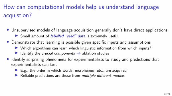
Segmenting verbs into stems and suffixes

• Data: orthographic forms of all verbs in the Penn Treebank• Task: split verbs into stems and suffixes:▶ Example: walk+ing, sleep+

• Excellent toy problem for learning models!• Locally-normalised Dirichlet-multinomial models⇒ Purely concatenative model that can’t capture phonological context⇒ Gets irregular forms and phonological changes wrong

• Maximum likelihood solution analyses each word as stem+∅ suffix⇒ sparse prior that prefers fewer stems and fewer suffixes

• Can we do this with a deep learning model?• Joint work with Sharon Goldwater and Tom Griffiths

26 / 78

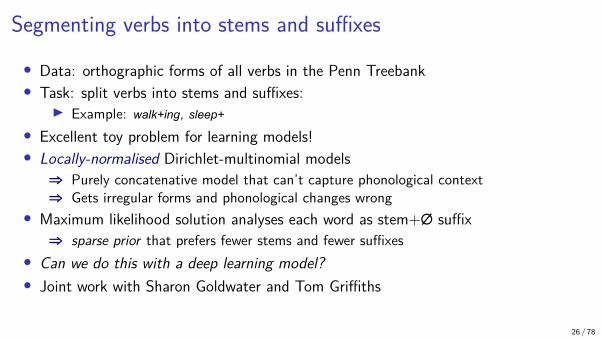
Posterior samples from WSJ verb tokensα = 0.1 α = 10−5 α = 10−10 α = 10−15

expect expect expect expectexpects expects expects expects

expected expected expected expectedexpecting expect ing expect ing expect ing

include include include includeincludes includes includ es includ esincluded included includ ed includ ed

including including including includingadd add add add

adds adds adds add sadded added add ed added

adding adding add ing add ingcontinue continue continue continue

continues continues continue s continue scontinued continued continu ed continu ed

continuing continuing continu ing continu ingreport report report report

reports report s report s report sreported reported reported reported

reporting report ing report ing report ingtransport transport transport transport

transports transport s transport s transport stransported transport ed transport ed transport ed

transporting transport ing transport ing transport ingdownsize downsiz e downsiz e downsiz e

downsized downsiz ed downsiz ed downsiz eddownsizing downsiz ing downsiz ing downsiz ing

dwarf dwarf dwarf dwarfdwarfs dwarf s dwarf s dwarf s

dwarfed dwarf ed dwarf ed dwarf edoutlast outlast outlast outlas t

outlasted outlast ed outlast ed outlas ted

27 / 78

Posterior samples from WSJ verb typesα = 0.1 α = 10−5 α = 10−10 α = 10−15

expect expect expect exp ectexpects expect s expect s exp ects

expected expect ed expect ed exp ectedexpect ing expect ing expect ing exp ectinginclude includ e includ e includ einclude s includ es includ es includ es

included includ ed includ ed includ edincluding includ ing includ ing includ ing

add add add addadds add s add s add sadd ed add ed add ed add ed

adding add ing add ing add ingcontinue continu e continu e continu econtinue s continu es continu es continu escontinu ed continu ed continu ed continu ed

continuing continu ing continu ing continu ingreport report repo rt rep ort

reports report s repo rts rep ortsreported report ed repo rted rep orted

report ing report ing repo rting rep ortingtransport transport transport transporttransport s transport s transport s transport stransport ed transport ed transport ed transport ed

transporting transport ing transport ing transport ingdownsize downsiz e downsi ze downsi zedownsiz ed downsiz ed downsi zed downsi zeddownsiz ing downsiz ing downsi zing downsi zing

dwarf dwarf dwarf dwarfdwarf s dwarf s dwarf s dwarf sdwarf ed dwarf ed dwarf ed dwarf ed

outlast outlast outlas t outla stoutlasted outlast ed outla sted

28 / 78

Adaptor grammar for stem-suffix morphology• Trees generated by an adaptor grammar are

defined by CFG rules• Unadapted nonterminals expand as in a PCFG• Adapted nonterminals expand in two ways:▶ generate a previously generated string (with

prob ∝ no. of times generated before), or▶ pick a rule and recursively expand its children

(as in PCFG)

Word

Stem

Chars

Char

t

Chars

Char

a

Chars

Char

l

Chars

Char

k

Suffix

Chars

Char

i

Chars

Char

n

Chars

Char

g

Chars

Char

#

• To generate a new Word from Adaptor Grammar:▶ reuse an old Word, or▶ generate a Stem and a Suffix, by

– reuse an old Stem (Suffix), or– generate a new Stem (Suffix) from PCFG

• Lower in the tree ⇒ higher in Bayesian hierarchy29 / 78

Outline






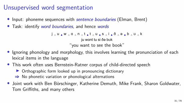
Unsupervised word segmentation• Input: phoneme sequences with sentence boundaries (Elman, Brent)• Task: identify word boundaries, and hence words

j Í u ▲ w Í ɑ Í n Í t ▲ t Í u ▲ s Í i ▲ ð Í ə ▲ b Í ʊ Í kju wɑnt tu si ðə bʊk

“you want to see the book”• Ignoring phonology and morphology, this involves learning the pronunciation of each

lexical items in the language• This work often uses Bernstein-Ratner corpus of child-directed speech▶ Orthographic form looked up in pronouncing dictionary⇒ No phonetic variation or phonological alternations

• Joint work with Ben Börschinger, Katherine Demuth, Mike Frank, Sharon Goldwater,Tom Griffiths, and many others

31 / 78

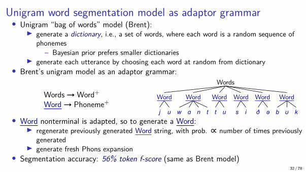
Unigram word segmentation model as adaptor grammar• Unigram “bag of words” model (Brent):▶ generate a dictionary, i.e., a set of words, where each word is a random sequence of

phonemes– Bayesian prior prefers smaller dictionaries

▶ generate each utterance by choosing each word at random from dictionary• Brent’s unigram model as an adaptor grammar:

Words→Word+Word→ Phoneme+

Words

Word

j u

Word

w ɑ n t

Word

t u

Word

s i

Word

ð ə

Word

b ʊ k• Word nonterminal is adapted, so to generate a Word:▶ regenerate previously generated Word string, with prob. ∝ number of times previously

generated▶ generate fresh Phons expansion

• Segmentation accuracy: 56% token f-score (same as Brent model)32 / 78

Adaptor grammar learnt from Brent corpus• Initial grammar

1 Words→Word Words 1 Words→Word1 Word→Phon1 Phons→Phon Phons 1 Phons→Phon1 Phon→D 1 Phon→G1 Phon→A 1 Phon→E

• Grammar learnt from Brent corpus16625 Words→Word Words 9791 Words→Word1575 Word→Phons4962 Phons→Phon Phons 1575 Phons→Phon134 Phon→D 41 Phon→G180 Phon→A 152 Phon→E460 Word→(Phons (Phon y) (Phons (Phon u)))446 Word→(Phons (Phon w) (Phons (Phon A) (Phons (Phon t))))374 Word→(Phons (Phon D) (Phons (Phon 6)))372 Word→(Phons (Phon &) (Phons (Phon n) (Phons (Phon d)))) 33 / 78

Undersegmentation errors with Unigram modelWords→Word+ Word→Phon+

• Unigram word segmentation model assumes each word is generated independently• But there are strong inter-word dependencies (collocations)• Unigram model can only capture such dependencies by analyzing collocations as

words (Goldwater 2006)

Words

Word

t ɛi k

Word

ð ə d ɑ g i

Word

ɑu t

Words

Word

j u w ɑ n t t u

Word

s i ð ə

Word

b ʊ k

34 / 78

Accuracy of unigram model

Number of training sentences

Toke

n f-s

core

0.0

0.2

0.4

0.6

0.8

1 10 100 1000 10000

35 / 78

Boundary precision of unigram model


Bou

ndar

y P

reci

sion

0.0

0.2

0.4

0.6

0.8

1.0

1 10 100 1000 10000

Boundary recall of unigram model


Bou

ndar

y R

ecal

l

0.0

0.2

0.4

0.6

0.8

1 10 100 1000 10000

36 / 78

Collocations ⇒ WordsSentence→Colloc+Colloc→Word+Word→Phon+

Sentence

Colloc

Word

j u

Word

w ɑ n t t u

Colloc

Word

s i

Colloc

Word

ð ə

Word

b ʊ k

• A Colloc(ation) consists of one or more words• Both Words and Collocs are adapted (learnt)• Significantly improves word segmentation accuracy over unigram model (76% f-score;≈ Goldwater’s bigram model)

37 / 78

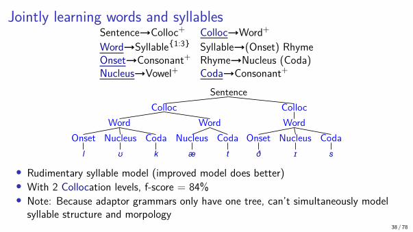
Jointly learning words and syllablesSentence→Colloc+ Colloc→Word+Word→Syllable{1:3} Syllable→(Onset) RhymeOnset→Consonant+ Rhyme→Nucleus (Coda)Nucleus→Vowel+ Coda→Consonant+

SentenceColloc

WordOnset

l

Nucleusʊ

Codak

WordNucleus

æ

Codat

CollocWord

Onsetð

Nucleusɪ

Codas

• Rudimentary syllable model (improved model does better)• With 2 Collocation levels, f-score = 84%• Note: Because adaptor grammars only have one tree, can’t simultaneously model

syllable structure and morpology38 / 78

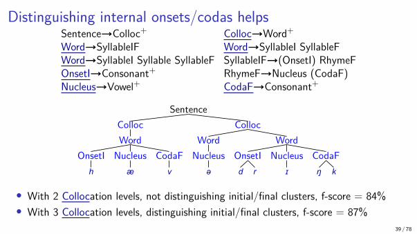
Distinguishing internal onsets/codas helpsSentence→Colloc+ Colloc→Word+Word→SyllableIF Word→SyllableI SyllableFWord→SyllableI Syllable SyllableF SyllableIF→(OnsetI) RhymeFOnsetI→Consonant+ RhymeF→Nucleus (CodaF)Nucleus→Vowel+ CodaF→Consonant+

SentenceCollocWord

OnsetIh

Nucleusæ

CodaFv

CollocWord

Nucleusə

WordOnsetId r

Nucleusɪ

CodaFŋ k

• With 2 Collocation levels, not distinguishing initial/final clusters, f-score = 84%• With 3 Collocation levels, distinguishing initial/final clusters, f-score = 87%

39 / 78

Collocations2 ⇒ Words ⇒ Syllables

Sentence

Colloc2

Colloc

Word

OnsetI

g

Nucleus

ɪ

CodaF

v

Word

OnsetI

h

Nucleus

ɪ

CodaF

m

Colloc

Word

Nucleus

ə

Word

OnsetI

k

Nucleus

ɪ

CodaF

s

Colloc2

Colloc

Word

Nucleus

o

Word

OnsetI

k

Nucleus

e

40 / 78

Accuracy of Collocation + Syllable model


Toke

n f-s

core

0.0

0.2

0.4

0.6

0.8

1.0

1 10 100 1000 10000

41 / 78

Accuracy of Collocation + Syllable model by word frequency


Acc

urac

y (f-

scor

e)

0.0

0.2

0.4

0.6

0.8

1.0

0.0

0.2

0.4

0.6

0.8

1.0

10-20

200-500

1 10 100 1000 10000

20-50

500-1000

1 10 100 1000 10000

50-100

1000-2000

1 10 100 1000 10000

100-200

1 10 100 1000 10000

42 / 78

F-score of collocation + syllable word segmentation model

Number of sentences

F-sc

ore

0.0

0.2

0.4

0.6

0.8

1.0

0.0

0.2

0.4

0.6

0.8

1.0

WH-word

light-verb

1 10 100 1000 10000

adjective

noun

1 10 100 1000 10000

adverb

preposition

1 10 100 1000 10000

conjunction

pronoun

1 10 100 1000 10000

determiner

verb

1 10 100 1000 10000

43 / 78

F-score of collocation + syllable word segmentation model

Number of sentences

F-sc

ore

0.0

0.2

0.4

0.6

0.8

1.0

0.0

0.2

0.4

0.6

0.8

1.0

0.0

0.2

0.4

0.6

0.8

1.0

a

it

wanna

1 10 100 1000 10000

book

put

what

1 10 100 1000 10000

get

that

with

1 10 100 1000 10000

have

the

you

1 10 100 1000 10000

is

this

1 10 100 1000 10000

44 / 78

Stem-suffix morphology and word segmentation

SentenceWord

Stemw a n

Suffix6

WordStemk l o z

SuffixI t

SentenceWord

Stemy u

Suffixh æ v

WordStemt u

WordStemt E l

Suffixm i

SentenceColloc

WordStemy u

WordStemh æ v

Suffixt u

CollocWord

Stemt E l

Suffixm i

45 / 78

Summary of word segmentation models• Word segmentation accuracy depends on the kinds of generalisations learnt.

Generalization Accuracywords as units (unigram) 56%+ associations between words (collocations) 76%+ syllable structure 84%+ interaction between

segmentation and syllable structure 87%

• Synergies in learning words and syllable structure▶ joint inference permits the learner to explain away potentially misleading

generalizations• We’ve also modelled word segmentation in Mandarin (and showed tone is a useful

cue) and in Sesotho (where jointly modeling morphology improves accuracy)46 / 78

Outline






Two hypotheses about language acquisition

1. Pre-programmed staged acquisition of linguistic components▶ Conventional view of lexical acquisition, e.g., Kuhl (2004)

– child first learns the phoneme inventory, which it then uses to learn– phonotactic cues for word segmentation, which are used to learn– phonological forms of words in the lexicon, …

2. Interactive acquisition of all linguistic components together▶ corresponds to joint inference for all components of language▶ can take advantage of synergies in acquisition▶ stages in language acquisition might be due to:

– child’s input may contain more information about some components– some components of language may be learnable with less data

48 / 78

Mapping words to referents

• Input to learner:▶ word sequence: Is that the pig?▶ objects in nonlinguistic context: dog, pig• Learning objectives:▶ identify utterance topic: pig▶ identify word-topic mapping: pig ⇝ pig

49 / 78

Frank et al (2009) “topic models” as PCFGs• Prefix sentences with possible topic marker, e.g.,

pig|dog• PCFG rules choose a topic from topic marker and

propagate it through sentence• Each word is either generated from sentence topic

or null topic ∅

Sentence

TopicpigTopicpig

TopicpigTopicpig

Topicpigpig|dog

Word∅

is

Word∅

that

Word∅

the

Wordpigpig

• Grammar can require at most one topical word per sentence• Bayesian inference for PCFG rules and trees corresponds to Bayesian inference for

word and sentence topics using topic model (Johnson 2010)50 / 78

AGs for joint segmentation and referent-mapping• Combine topic-model PCFG with word segmentation AGs• Input consists of unsegmented phonemic forms prefixed with possible topics:

pig|dog ɪ z ð æ t ð ə p ɪ g

• E.g., combination of Frank “topic model”and unigram segmentation model▶ equivalent to Jones et al (2010)

• Easy to define other combinations of topicmodels and segmentation models

Sentence

TopicpigTopicpig

TopicpigTopicpig

Topicpigpig|dog

Word∅ɪ z

Word∅ð æ t

Word∅ð ə

Wordpigp ɪ g

51 / 78

Collocation topic model AG

Sentence

Topicpig

Topicpig

Topicpig

pig|dog

Colloc∅

Word∅

ɪ z

Word∅

ð æ t

Collocpig

Word∅

ð ə

Wordpig

p ɪ g

• Collocations are either “topical” or not• Easy to modify this grammar so▶ at most one topical word per sentence, or▶ at most one topical word per topical collocation

52 / 78

Experimental set-up• Input consists of unsegmented phonemic forms prefixed with possible topics:

pig|dog ɪ z ð æ t ð ə p ɪ g

▶ Child-directed speech corpus collected by Fernald et al (1993)▶ Objects in visual context annotated by Frank et al (2009)

• Bayesian inference for AGs using MCMC (Johnson et al 2009)▶ Uniform prior on PYP a parameter▶ “Sparse” Gamma(100, 0.01) on PYP b parameter

• For each grammar we ran 8 MCMC chains for 5,000 iterations▶ collected word segmentation and topic assignments at every 10th iteration during last

2,500 iterations⇒ 2,000 sample analyses per sentence

▶ computed and evaluated the modal (i.e., most frequent) sample analysis of eachsentence

53 / 78

Does non-linguistic context help segmentation?Model word segmentation

segmentation topics token f-scoreunigram not used 0.533unigram any number 0.537unigram one per sentence 0.547

collocation not used 0.695collocation any number 0.726collocation one per sentence 0.719collocation one per collocation 0.750

• Not much improvement with unigram model▶ consistent with results from Jones et al (2010)

• Larger improvement with collocation model▶ most gain with one topical word per topical collocation

(this constraint cannot be imposed on unigram model)54 / 78

Does better segmentation help topic identification?• Task: identify object (if any) this sentence is about

Model sentence referentsegmentation topics accuracy f-score

unigram not used 0.709 0unigram any number 0.702 0.355unigram one per sentence 0.503 0.495

collocation not used 0.709 0collocation any number 0.728 0.280collocation one per sentence 0.440 0.493collocation one per collocation 0.839 0.747

• The collocation grammar with one topical word per topical collocation is the onlymodel clearly better than baseline

55 / 78

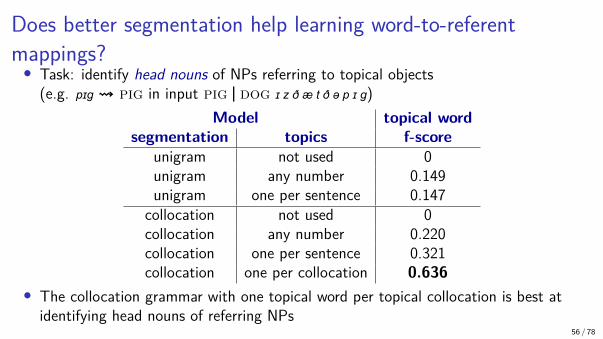
Does better segmentation help learning word-to-referentmappings?• Task: identify head nouns of NPs referring to topical objects

(e.g. pɪg ⇝ pig in input pig | dog ɪ z ð æ t ð ə p ɪ g)Model topical word

segmentation topics f-scoreunigram not used 0unigram any number 0.149unigram one per sentence 0.147

collocation not used 0collocation any number 0.220collocation one per sentence 0.321collocation one per collocation 0.636

• The collocation grammar with one topical word per topical collocation is best atidentifying head nouns of referring NPs

56 / 78

Summary of grounded learning and word segmentation

• Word to object mapping is learnt more accurately when words are segmented moreaccurately▶ improving segmentation accuracy improves topic detection and acquisition of topical

words• Word segmentation accuracy improves when exploiting non-linguistic context

information▶ incorporating word-topic mapping improves segmentation accuracy (at least with

collocation grammars)⇒ There are synergies a learner can exploit when learning word segmentation and

word-object mappings• Caveat: Need to confirm results using different models

57 / 78

Other topics investigated with Adaptor Grammars• The role of social cues such as eye-gaze▶ Eye gaze (particularly from child) is strong topicality cue▶ Useful for identifying word referents▶ Not useful for word segmentation

• Stress and Phonotactics in English▶ Learns Unique Stress Constraint from unsegmented data (Yang 2004)▶ Additive interaction: model with both stress and phonotactics is better than with just

one• Monosyllabic “function words” are useful cues for word and phrase boundaries▶ Model inspired by Shi’s experimental work▶ Increases word segmentation f-score from 0.87 to 0.92▶ After about 1,000 sentences, model overwhelming prefers to attach “function words”

at left phrasal periphery• Results should be confirmed with other kinds of models!

58 / 78

Outline


Segmentation models




59 / 78

Phonological alternation• Words are often pronounced in different ways depending on the context• Segments may change or delete▶ here we model word-final /d/ and /t/ deletion▶ e.g., /w ɑ n t t u/ ⇒ [w ɑ n t u]

• These alternations can be modelled by:▶ assuming that each word has an underlying form which may differ from the observed

surface form▶ there is a set of phonological processes mapping underlying forms into surface forms▶ these phonological processes can be conditioned on the context

– e.g., /t/ and /d/ deletion more common when following segment is consonantal▶ these processes can also be nondeterministic

– e.g., /t/ and /d/ don’t always delete even when followed by a consonant• Joint work with Joe Pater, Robert Staubs and Emmanuel Dupoux

60 / 78

Harmony theory and Optimality theory• Harmony theory and Optimality theory are two models of linguistic phenomena

(Smolensky 2005)• There are two kinds of constraints:▶ faithfulness constraints, e.g., underlying /t/ should appear on surface▶ universal markedness constraints, e.g., ⋆tC

• Languages differ in the importance they assign to these constraints:▶ in Harmony theory, violated constraints incur real-valued costs▶ in Optimality theory, constraints are ranked

• The grammatical analyses are those which are optimal▶ often not possible to simultaneously satisfy all constraints▶ in Harmony theory, the optimal analysis minimises the sum of the costs of the violated

constraints▶ in Optimality theory, the optimal analysis violates the lowest-ranked constraint

– Optimality theory can be viewed as a discrete approximation to Harmony theory61 / 78

Harmony theory as Maximum Entropy models• Harmony theory models can be viewed as Maximum Entropy a.k.a. log-linear a.k.a.

exponential models

Harmony theory MaxEnt modelsunderlying form u and surface form s event x = (s, u)Harmony constraints MaxEnt features f(s, u)constraint costs MaxEnt feature weights θHarmony −θ · f(s, u)

P(u, s) =1Zexp−θ · f(s, u)

62 / 78

Learning Harmonic grammar weights

• Goldwater et al 2003 learnt Harmonic grammar weights from (underlying,surface)word form pairs (i.e., supervised learning)▶ now widely used in phonology, e.g., Hayes and Wilson 2008

• Eisenstadt 2009 and Pater et al 2012 infer the underlying forms and learn Harmonicgrammar weights from surface paradigms alone• Linguistically, it makes sense to require the weights −θ to be negative since Harmony

violations can only make a (s, u) pair less likely (Pater et al 2009)

63 / 78

Integrating word segmentation and phonology

• Prior work has used generative models▶ generate a sequence of underlying words from Goldwater’s bigram model▶ map the underlying phoneme sequence into a sequence of surface phones

• Elsner et al 2012 learn a finite state transducer mapping underlying phonemes tosurface phones▶ for computational reasons they only consider simple substitutions

• Börschinger et al 2013 only allows word-final /t/ to be deleted• Because these are all generative models, they can’t handle arbitrary feature

dependencies (which a MaxEnt model can, and which are needed for Harmonicgrammar)

64 / 78

Liang/Berg-Kirkpatrick unigram segmentation model• Liang/Berg-Kirkpatrick et al MaxEnt unigram model with double exponential prior:

P(s | θ) =1Zexp(−θ · f(s)) exp(−|w|d)︸︷︷︸

length penalty

• Feature function f(s) includes word id, word prefix/suffix features, etc.▶ We extend s to be an surface/underlying pair x = (s, u), and allow P(x) to condition

on neigbouring surface segments• Partition function Z▶ Doesn’t normalise “length penalty” (so model is deficient)▶ Sums only over substrings in the training corpus (not all possible strings)

• “Length penalty” exponent d needs to be tuned somehow!• Segmentation accuracy rivals adaptor grammar model with phonotactics and

collocations▶ How can it do so well without modelling supra-word context?

65 / 78

Sensitivity to word length penalty factor d

0.3

0.4

0.5

0.6

0.7

0.8

0.9

1.4 1.5 1.6 1.7

Word length penalty

Su

rfa

ce

to

ke

n f-s

co

re

Data

Brent

Buckeye

66 / 78

A joint model of word segmentation and phonology

• Because Berg-Kirkpatrick’s word segmentation model is a MaxEnt model, it is easyto integrate with Harmonic Grammar/MaxEnt phonology• P(x) is a distribution over surface form/underlying form pairs x = (s, u) where:▶ s ∈ S, where S is the set of length-bounded substrings of D, and▶ s = u or s ∈ p(u), where p is either word-final /t/ or word-final /d/ deletion

• Example: In Buckeye data, the candidate (s, u) pairs include([l.ih.v], /l.ih.v/), ([l.ih.v], /l.ih.v.d/) and ([l.ih.v], /l.ih.v.t/)these correspond to “live”, “lived” and the non-word “livet”

67 / 78

Probabilistic model and optimisation objective• The probability of word-final /t/ and /d/ deletion depends on the following word ⇒

distinguish the contexts C = {C,V,#}

P(s, u | c, θ) ∝1Zc

exp(−θ · f(s, u, c))• We optimise an L1 regularised log likelihood QD(θ), with the word length penalty

applied to the underlying form uQ(s | c, θ) =

∑u:(s,u)∈X

P(s, u | c, θ) exp(−|u|d)

Q(w | θ) =∑

s1...sℓs.t.s1...sℓ=w

ℓ∏j=1

Q(sj | c, θ)

QD(θ) =n∑

i=1logQ(wi | θ)− λ ||θ||1

68 / 78

MaxEnt features• Here are the features f(s, u, c) where s = [l.ih.v], u = / l.ih.v.t/ and c = C▶ Underlying form lexical features: A feature for each underlying form u. In our

example, the feature is <U l ih v t>. These features enable the model to learnlanguage-specific lexical entries.There are 4,803,734 underlying form lexical features (one for each possible substringin the training data).

▶ Surface markedness features: The length of the surface string (<#L 3>), the numberof vowels (<#V 1>), the surface prefix and suffix CV shape (<CVPrefix CV> and<CVSuffix VC>), and suffix+context CV shape (<CVContext _C> and<CVContext C _C>).There are 108 surface markedness features.

▶ Faithfulness features: A feature for each divergence between underlying and surfaceforms (in this case, <*F t>).There are two faithfulness features.

69 / 78

L1 regularisation and sign constraints

• We chose to use L1 regularisation because it promotes weight sparsity (i.e., solutionswhere most weights are zero)• Sign constraints we explored:▶ Lexical entry weights must be positive (i.e., you learn what words are in the language)▶ Harmony faithfulness and markedness constraint weights must be negative

70 / 78

Experimental results: Data preparation procedure• Data from Buckeye corpus of conversational speech (Pitt et al 2007)▶ provides an underlying and surface form for each word

• Data preparation as in Börschinger et al 2013▶ we use the Buckeye underlying form as our underlying form▶ we use the Buckeye underlying form as our surface form as well …▶ except that if the Buckeye underlying form ends in a /d/ or /t/ and the surface form

does not end in that segment our surface form is the Buckeye underlying form withthat segment deleted

• Example: if Buckeye u = / l.ih.v.d/ “lived”, s = [l.ah.v]then our u = / l.ih.v.d/ , s = [l.ih.v]• Example: if Buckeye u = / l.ih.v.d/ “lived”, s = [l.ah.v.d]

then our u = / l.ih.v.d/ , s = [l.ih.v.d]

71 / 78

Data statistics• The data contains 48,796 sentences and 890,597 segments.• The longest sentence has 187 segments.• The “gold” segmentation has 236,996 word boundaries, 285,792 word tokens, and

9,353 underlying word types.• The longest word has 17 segments.• Of the 41,186 /d/s and 73,392 /t/s in the underlying forms, 24,524 /d/s and 40,720

/t/s are word final, and of these 13,457 /d/s and 11,727 /t/s are deleted.• All possible substrings of length 15 or less are possible surface forms S• There are 4,803,734 possible word types and 5,292,040 possible surface/underlying

word type pairs.• Taking the 3 contexts derived from the following word into account, there are

4,969,718 possible word+context types.• When all possible surface/underlying pairs are considered in all possible contexts

there are 15,876,120 possible surface/underlying/context triples.72 / 78

Overall segmentation scores

Börschinger et al. 2013 Our modelSurface token f-score 0.72 0.76 (0.01)Underlying type f-score — 0.37 (0.02)Deleted /t/ f-score 0.56 0.58 (0.03)Deleted /d/ f-score — 0.62 (0.19)

• Underlying type or “lexicon” f-score measures the accuracy with which the underlyingword types are recovered.• Deleted /t/ and /d/ f-scores measure the accuracy with which the model recovers

segments that don’t appear in the surface.• These results are averaged over 40 runs (standard deviations in parentheses) with the

word length penalty d = 1.525 applied to underlying forms

73 / 78

Conclusions from MaxEnt joint models of segmentation andphonology

• Globally-normalised MaxEnt model doesn’t require a tree structure⇒ Can capture contextual dependency in phonological alternation

• No need to calculate partition function over all possible underlying/surface forms• Liang/Berg-Kirkpatrick double-exponential word length penalty works extremely well▶ How do we set the d parameter?

74 / 78

Outline


Segmentation models




75 / 78

Outline


Segmentation models




76 / 78

Summary

• For toy examples, it’s possible to learn abstract grammatical properties and lexicalentries from positive evidence alone• Bayesian segmentation models can solve word segmentation problems▶ Adaptor grammars can find complex hierachical structure

• Maximum entropy models can jointly learn word segmentation and (simple) phonology• Neural networks don’t need or produce explicit linguistic representations

77 / 78

Challenges for future work

• How are deep neural networks related to linguistic generalisations?▶ Deep networks can learn linguistic generalisations extremely well▶ But they can also learn apparently random patterns▶ Smolensky’s Harmony Theory and Tensor Product Representations (?)

• Technology can get ahead of scientific understanding▶ The steam engine was developed centuries before statistical mechanics▶ Why can’t a heat engine extract all the energy ⇒ entropy

78 / 78

Documents

Computational Models of Hidden Structure Learning and