Embed Size (px)
Citation preview

J . Mol. Bioi. (1994) 235, 1501-1531
Hidden Markov Models in Computational Biology Applications to Protein Modeling
Anders Krogh'f, Michael Brown', I. Saira Mian' Kiminen Sjolander' and David Hausder'S
'Computer and Information Sciences 2Sinsheimer Laboratories
University of California, Santa Cruz, C A 95064, U.S .A.
Ridden .Markov Models (HMMs) are applied t.0 the problems of statistical modeling, database searching and multiple sequence alignment of protein families and protein domains. These methods are demonstrated on the globin family, the protein kinase catalytic domain, and the EF-hand calcium binding motif. In each case the parameters of an HMM are estimated from a training set of unaligned sequences. After the HMM is built, it is used to obtain a multiple alignment of all the training sequences. It is also used to search the
. SWISS-PROT 22 database for other sequences. that are members of the given protein family, or contain the given domain. The Hi" produces multiple alignments of good quality that agree closely with the alignments produced by programs that incorporate three- dimensional structural information. When employed in discrimination tests (by examining how closely the sequences in a database fit the globin, kinase and EF-hand HMMs), the '\ HMM is able to distinguish members of these families from non-members with a high degree '
of accuracy. Both the HMM and PROFILESEARCH (a technique used to search for relationships between a protein sequence and multiply aligned sequences) perform better in these tests than PROSITE (a dictionary of sites and patterns in proteins). The HMM appecvs to have a slight advantage over PROFILESEARCH in terms of lower rates of false negatives and false positives, even though the HMM is trained using only unaligned sequences, whereas PROFILESEARCH requires aligned training sequences. Our results suggest the presence of an EF-hand calcium binding motif in a highly conserved and evolutionary preserved putative intracellular region of 155 residues in the a-l subunit of L-type calcium channels which play an important role in excitation-contraction coupling. This region has been suggested to contain the functional domains that are typical or essential for all L-type calcium channels regardless of whether they couple to ryanodine receptors, conduct ions or both.
Keywords: hidden Markov models; multiple sequence alignments; globin; kinase; EF-hand
\
1. Introduction hidden Markov models (HMMdl to the DrobiemS of The rate of generation of sequence data in recent
years provides abundant opportunities for the development of new approaches to problems in computational biology. In this paper, we apply
statistical modeling, 'database searihing, and multiple alignment of protein families and protein domains. To demonstrate the method, we examine three protein families. Each family consists of a set of proteins that have the same overaIl three-dimen- - sional structure but widely divergent. sequences. t Present address: Electronics Institute, Build 349, Features of the sequences that are determinants of folding, structure and function should be present as
$ Author to whom all correspondence should be conserved elements in the family of sequences. We
8 Abbreviations HMM, hidden Marko,. ,,,dels; length from 130 to 170 residues (with few excep- ' m, Expectetion-Maximization; ML. maximum tions) and two domains, the protein kinase catalytic
like€ihood; MAP, maximum a posten'wi; hTL-score. domain (250 to 300 residues) and the EF-hand negative log likelihood score. caicium-binding motif (29 residues). The same
1.50 1
Technical University of Denmark, 2800 Lyngby. Denmark.
oddreased. consider t.he globins, whole proteins ranging in
CO22-2836/94!031301-31 $08.00!0 'r; 199-1 .-\cdcrnir I'rpss Limited

1502 IIidden JZarkoz: :Models
approach can be used to model families of nucleic acid sequences as well (Krogh et al.. 19936).
A hidden Markor model (Rabiner, 1989) describes a series of observations by a "hidden'' stochastic process, a Markov process. In speech recognition. where HMMs hare been used extensively, the observations are sounds forming a word. and a model is one that by i t s hidden random process generates these sounds with high probability. Every possible sound sequence can be generated b.v the model with some probability. Thus: the model defines a probabiIity distribution over possible sound sequences. X good word model would assign high probability to all sound sequences t.hat are likely utterances of the word it models. and low probability to any other sequence. In this paper we propose an HM31 similar to the ones used in speech recognition to model protein families such as globins and kinases. In speech recognition. the '-alphabet" from which words are constructed could be the set of phonemes valid for a particular language: in protein modeling. the alphabet we use is the 20 amino acids from which protein molecules are constructed. t7'here t.he observations in speech recognit.ion are words. or strings of phonemes. in protein modeling the observations are strings of a.mino acids forming the primary sequence of a protein. A model for a set of proteins is one that assigns high probability to the sequences in that particular set.
The HYY we build identifies a set of positions 'fhat describe the (more or less) conserved first-order &ructure in the sequences from a given family of proteins. In biological terms. this corresponds to identifl-ing the core elements of homologous molecules. The model provides additional informa- tion, such as the probability of initiating an inser- tion at any position in the model and the probability of extending it. The structure of the madel is similar to that of a profile (Waterman & Perlu-itz, 1986: Barton Q Sternberg, 1990: (;rihsko\- et al., 1990: Bowie et ai.. 1991: Iiithy et nl.. 1991). but slightlv more general. Onw we have built the model from unaligned sequences. we can generate a multiple alignment of the sequences using a dynamic programming method. By employing it for database searching, the model can be used to tlis- criminate sequences that belong to a given family from non-members. Finally. we can study the model we have found directly. and see what i t reveals about the common structure underlying the various sequences in the famill-.
Our method of multiple alignment differs quite markedly from conventional techniques. which are usually based on painvise alignments generated by d y n m i c programming. schemes (Waterman. 1989: Fend & DootittIe, 1987; Barton, 1990: Subbiah & Harrison, 1989). The alignments produced by these methods often depend strongl? on the particular vaiues of t h e pa.rameters required by the method. in particular the gap penalties (Vingron & Argos. 1991). Furthermore, a given set of sequences is likely to possess both fairly conserved regions and
highly variable regions, vet conventional global methods assign identical penalties for all of the sequences. Substitutions, insertions, or deletions in a region of high conservation should ideally be penalized more than in a variable region, and Some kinds of substitutions should be penalized differ- ently in one position compared to another. That is one of the motivations for the present work. The statistical model we propose corresponds to multiple alignment with variable. position-dependent gap penalties. Furthermore, these penalties are in large part learned from the data itself. Essentially, we build a statist.ical model during the process of multiple alignment. rather than leal-ing this as a separat.e task to be done after the alignment is completed. \Ye believe the model should guide the alignment as much as the alignment determines the model.
We are not the first group to employ hidden Markov models i n computationa.i biology. Lander & Green (198T) used hidden Markov models in the construction of genetic linkage maps. Ot.her work employed HJIUs to distinguish coding from non- coding regions in DSA (Churchill, 1989). Later, simple HJIJIs were used in conjunction with the EM algorithnl to model certain protein-binding sites in DSA (Lawrence Q R.eilly, 1990; Cardon & Stormo, 1992) and. more recently, to model the S-caps and C'-caps of alpha helices in proteins (D. Morris, unpublished results). These applications of HMNs and the EJl (Espertation-Maximization) algorithml including our own. presage a more widespread use of this technique in rotnputational biology. During the time that we have been developing this approach. several related efforts hare come to our attention. One is that of \illite. Stu1t.z and Smith (White et nl.. 1991: Stnltz et d.. 1993), who use HMMs to model protein superfamilies. This work is more ambitious than our o w l . since superfamilies are harder to characterize than families. I t is not get dear how successful their work has been since no results are reported for sequences not in the training set. If there are weaknesses in their method. it is possible that these are due to the use of handcrafted models and wliance on prealigned data for parameter esti- mation. T n contrast. our models have a simple regular structure. and we are able to estimate all the parameters of these models. including the size of the model directly from unaligned training sequences. Interestingly enough, they independently propose an alternate H l i N state structure similar to oursi i n section 6.3 of their paper (White et al.. 1991). where they discuss the relationship of their work to Bowie and co-workers (Bowie et al., 1991): but they do not pursue this further. Tt is possible t.hat the txpe of models we use may work better for charac- terizing superfamilies than those investigated by \Vhite et 01. However. it is more likely that they are too simple. and that richer and more varied state

Hidden Markov Models 1503
Figure 1. The model.
structure along the lines they propose is required for this problem. We recently found that Asai et al. (1993) ha.ve applied HMMs to the problem of predicting the secondary structure of proteins, obtaining prediction rates that are competit ive with previous methods in some cases. In addition, Tanaka et al. (1993) also discuss the relationship between t h e HMM method for obtaining multiple alignments and previous methods. Finally. in work most closely related to our own, since the t ime ne presented a preliminary report on this work (Haussler Br Krogh, 1992; see also Haossler el ai.. 1992): BaIdi el ai. (1993) have fur ther demonstrated the usefulness of this technique by producing multiple aiignments for immunoglobins and protease as we11 as globins and kinasest .
2. Methods (a) H Y , W architecture
Consider a family of protein sequences that all have a common three-dimensional structure. for rsample the globins. The common structure in these sequences can be defined as a sequence of positions in spacu where amino acids occur. In the case of globins. whosr structure contains principally z-helices. the 1% or so helical posi- tions have been named A I . -12. . . .. A 16. HI. . . . etc.. where the letter denotes the n-helis. and the number indicates the location within that z-helix (see for esample Bashford et 01.. 1985). For each of these positions there is a (distinct) probability distribution over the 20 amino acids that measures the likelihood of each amino acid occurring in that position in a typiral g1,obin. as well as - the p m b a b i l e that there is no amino acid in that posi- tion (Le. that a sequence belonging to this family may have a gap at that position in a multiple alignment). These have been called profiles (Waterman 8: Perlwitz. 1986; Barton 8. Sternberg. 1990: Gribskov cl 01.. 19% Bowie et el.. 1991; Liithy et al.: 1991). A profile of globins can be thought of as a statistical model for the family of globins, in that for any sequence of amino aeids. i t defines a probability for that sequence:in such a way that globin sequences tend to have much higher probabilities than non-globin sequences.
The type of hidden Markov model we use as a statistical model for a protein family can be viewed as a generalized profile. However. instead of describing the HM31 directly
. . .
t They have dere1op.I a variant of the n~rthod described here that employs a gradient cirzwnt training algorithm in plare of the EM algorithm.
i n terms of the probability it assigns to each protein sequence. we find that it is easier to first think of an HMM as a structure that generates protein sequences by a random process. This structure and corresponding random process is illustrated in Figure 1 and can be described as follo~vs.
The main line of the HMM contains a sequence of Y states. \vhich we call match states, corresponding to psi- tions in a protein or columns in a multiple alignment (M equals 1 i n Fig. I ). Each of these states can generate a . letter x from the %letter amino acid alphabet. according to a distribution 9(.rlmk). k = 1 . . . N . The notation 9 (.rlmt) means that each of the match states m,. 1 S k S .II. haw distinct distributions. For each match state mk, there is a delete state dk that does not produce anv amino acid but is a '-dummy" state used to skip mk. Finally, there BIP a total of .I1 + 1 insert states to either side of tbe match states which generate amino acids in exactly tb same way as the match states. but use probability distri- butions 9 ( . r l i k ) . In Figure 1. match. delete and insert states are shown as boxes. circles and diamonds, respec- tively. For convenience, we have added a dummy -'HE(;IS" state and a dummy "EXD" state, denoted mo and mM- I . respectively. which do not produce any amino acid.
From each state. there are three possible transitions to other states. also shown in Figure 1. Transitions into match or delete states always move forward in the model, whereas transitions into insert states do not. Sote that nlultiple insertions between match states can occur, since the self-loop on the insert state allows a transition from the insert state to itself. The transition probability from state q to state r is called 9 ( r lq) . Our notation is summar- ized in Table 1.
A sequence can be generated by a "random walk" through the model as follows: Commencing at state mo (BEGIS). choose a transition to m,. d,. or io randomly
Table 1 Notation
X Amino acid
L 3 Sequence of amino acids (s= rl . . .xL)
Length of sequence 9. Stnte in HMM tmlh A sequence of states. q, . . . qN .Y Somber of states in a yat.h .I1 Length of model m. i. d Jktrh. insert, and delete states ]no. nly+, B(.elg)
Begin and end s t a t e Probability distribution of amino acids in
g(rlql Probability of a transition from sbatr q to r state q

1504 Hidden Markov Models
according to the probabilities 9 ( m , l m o ) , 9 (dllmo), and 9 (iolmo). If m, is chosen, generate the first amino acid rl from the probability distribution b(z)m,), and choose a transition to the next state according to probabilities F (-]ml), where * indicates any possible next state. If this next state is the insert state i,, then generate amino acid zz from B(zli,) and select the next state from 3-(-lil). If delete Id2) is chosen next, generate no amino acid, and choose the next state from Y(-ld2). Continue in this manner all the way to the END state, generating a sequence of amino acids zl. z2 . . . z, by following a path of states qo. ql . . . qN, qN+l through the model, where go = m, (the BEGIN state) and qN+ I = mM+l (the Eh’D state). Because the delete states do not produce any amino mid, N is larger than or equal to L. If qi is a match or i n s e r t state, we define I(i) to be the index in the sequence x l . . . zL of the amino acid produced in state pi. The probability of the event that t.he path qo . . , q N + , is taken and the sequence rl . . . x, is generated is
Prob(z, . . . q , qo . . . qn+ I model) N
=F(mN+IIqN) X n~(qiIqi-l)B(~,~i~Iqi), (1) i- 1
where we set B(zIMlqi) = 1 if qi is a delete state. The probabiiity of any sequence zl . . . tL of amino acids is a sum over all possible paths that could produce that sequence. which we write as follows:
Prob(z, . . . zLlmodel)
= Prob(z, ... z,, qo ,..‘qN+llmcdel). (2)
In this way a probability distribution on the space of pquences is defined. The goal is to find a model (Le. a &roper model length and probability parameters) that accurately describes a Eamily of proteins by assigning large probabilities to sequences in that family.
This particular structure for the HMM was chosen because i t is the simplest model that captures the struc- tural intuition of a protein: (a) a sequence of positions. each with i t s own distribution over the amino acids: (b) the possibility for either skipping a position or inserting extra amino acids between consecutive positions; and (c) allowing For the possibility that continuing an insertion or deletion is more likely than starting one. This choice appears to have worked well for modeling t.he protein famiiies that we hsve examined, but othertypes of HMMs may be better at other tasks (e.g. the more elaborate models for protein superfamilies used by White et ai.. 1991; Stultz el al., 1993). The important feature of the HMM method is i t s generality. One can choose any struc- ture for the states and transitions that is appropriate for the problem at hand. Examples of more general HMIY architectures are given in sections (d) and (e). below.
P.lhrl0 ... l N S 1
(b) Estimating the parameters of an H M N f r o m training sequences
AI1 the parameters in the HMM (i.e. the transition probabilities and the amino acid distributions) could in principle be chosen by hand. from an existing alignment of protein sequences, as in Gribskov et al. (1990), White el al. (1991). Stultz et al. (1993), or from information about the threedimensional structure of proteins, as in Bowie et al. (19911, White et al. (1991), Stultz et aZ. (1993). The novel approach we take is to “learn” the parameters entirely automatically from a set of unaligned primary sequences, using an EM algorithm. This approach can in
principle find the model t ha t best describes a given set of sequences.
Given a set of training sequences S( l) , . . ., s ( n ) , one can see how well a model fits them by calculating the prob- ability that it generates them. This probabi1it.y is simply a product of terms of the form given by equation (2), i.e.
n Prob(sequenceslmode1) = n Prob(sU)fmodel), (3) . .
j - 1
where each term Prob(s(j)l model) is calcul&ed by substi- tuting z1 . . . xL = ~ ( j ) in equation (2). This is cal led the likelihood of the model. One would‘like this value to be high. The maximum likelihood (PIIL) method of model estimation is to find the mode1 that maximizes the likeli- hood (3).
An alternate approach to ML estimation is the maxi- mum’ a posferiuri (MAP) approach. Here, we assume a prior probability d h i b u t i o n over all possible parameters of the model embodying prior beliefs on what a model should be like. This can then be used to “penalize” models that are known to be bad or uninteresting. We discuss this further in Rrogh et ul. (1993~). In MAP estimation? we t ry to maximize the posterior probability of the mode1 given the sequences. Using Bayes rule. the posterior probability can be calculated as
Prob(mode1lsequences)
- - Prob(sequenceslmode1) Prob(mode1) Prob(sequences) . (4)
Here Prob(mode1) is the prior probability distribution, and Prob(sequences) can be viewed as a normalizing constant. Since this normalizing constant is independent of the model. MAP estimation is equivalent to maximizing
Prob(sequencelmode1) Prob(mode1). t5)
over all possible models. The MAP approach is closely related to minimum description length (Jurka & Milosa\-ljevic. 1991) and minimum mesage length .(Allison el al.. 1992) methods.
There is no known efficient way to directly calculate the best HMM model either in the YL or MAP sense, However. there are algorithms that given an arbitrary starting point find a local maximum by iteratively re-estimating the model in such a way that the likelihood (or the posterior probabi1it.y) increases in each iteration. The most common one is the Baum-Welch or forward- backward algorithm (Rabiner. 1989; Lawrence & Reilly, 1990), which is a version of the general EM method often used in statistics (Dempster et al.. 1977). The process of the EM algorithm can be viewed as an iterative adap- tation of the model to fit the training sequences. The steps in this process can be summarized as follows:
(1) An initial model is created by assigning values to the transition probability Y (rip) and the amino acid generation probability P (xlq) for each 2, q and r, where z is one of the 20 amino acids and q and r are states in the HMN connected by a transition arc. If one already knows some features present in the sequences, or constraints on the sequences, these may sometimes be encoded in the initial model. The current model is set to this initial model.
(2) Csing the current model, all possible paths for each training sequence are considered in order to get a new estimate J (514) of-the transition probability 9 ( r l g ) and a new estimate b(zlq) of the amino acid generation probability P(z(q) for each z. q and r. The transition
Hidden Markov Models 1 ou5
probability estimate g ( r l q ) is obtained by counting the number of times a transition is made from state q to 7, for all paths of all training sequences, wsighted by the prob- ability of the path. The estimate P(zIq) is made in a similar manner. by counting the number of times the amino acid x is aligned to the state q.
(3) In the next step of ML estimation, a new current model is created- by simply replacing Y (714) by Y ( r l q ) and P(z1q) by b(rlq) for e3ch 2, q an! r. In MAP EM estimation, the parameters 9 (s lq) and d(zJq) are further modified by considering the prior probability of the model before they are used to replace the old parameters.
(4 ) Steps (2) and (3) are repeated until t.he parameters of the current model change only insignificantly.
Since the quality of the current model (as measured by equations (3} or (5)) incre+ses in each iteration, and no model is arbitrarily good, the process eventually termi- nates and produces a model that is, at least locally, the best model for the training sequences t.o within some specified precision of the parameters (Dempster el a.1.. 1975). Typically. this occurs very rapidly (e.g. in less than 10 iterations) even for large models and large sets of training sequences.
The main computzitional bottleneck in the algorithm is step (2). since individualiy examining each possible path for every training sequence would generally take time exponential in the length of the longest training sequence.
. .However, i t is possible to use a dynamic programming technique known as the forward-backward procedure to speed up this step. Using this method, the new parameter estimates can be calculated in time proportional to t,he number of states in the model multiplied by the total length of all the training sequences. Details are given in the excellent tutorial article on HMMs by Rabiner (1989).
“he forward part of the forward-backward procedure can also be used to efficiently compute. -log Prob(sequencetmode1). the negative logarithm of the probability of a sequence.given the model (as defined in equation (2)), without summing over all possible paths for the sequence (Rabiner, 1989). We call this the negative log likelihood (SLL)-score of the sequence. The average hTLL-acore of a training sequence is inversely related to the likelihood of the model, given by equation (3). and hence serves as a numerical measure of progress for each iteration of the EM procedure. The KLL-score can also be used to evaluate how well the model fits a novel “test.” sequence not present in the training set, as described in section (c) below.
(c) The Viferbi ctlgwithm and mzclliple alignmenf f r m an H M M
The forward-backward procedure is related to the dynamic programming technique used to align one sequence. to another, or more generally to align a sequence to a profile. A ,variant of the forward-backward procedure known as the Viterbi algorithm is similar to the standard profile alignment algorithm (Waterman & Perlwitz, 1986; Barton k Sternberg, 1990; Gribskov et al.. 1990). Instead of calculating t.he ELL-score for a sequence, which impli- citly involves all possible paths for that sequence through the model, the Viterbi algorithm computes the negative logarithm of the probability of the single most likely path for the sequence. We can write this as
- log max Prob(s, pathlmodel), (6)
where Prob(s. psthlmodel) is given in equation (1). with u = z1 . . . rL and path = qo . . . qN+ l . Instead of first maxi-
pork
mizing the probability of the path and then taking the negative logarithm. i t is convenient (and equivalent) to simply minimize the negative logarithm of the probability over all paths. This minimum we will call the distance from the sequence to the model,
dist(s. model) = min {-log &ob(s, pathlmodel)) parh
N + 1
= min. 2 [ - l o g ~ ( q i I q i - l ) - l o g ~ ( z , , , t g , ) ~
This distance from a sequence to a model is analogous to the standard “edit distance’’ from one sequence to another (nit,h gap penalties), see e.g. Waterman (1989), but is perhaps more related to the distance from a sequence to’a profile. The term -log9(rl~nlqi) represents a penalty for aligning the amino acid r,,, to the position represented by state pi in the model. The term - logF(qi lqi- l ) corresponds to a penalty for using the transition from to pi in the model. If this is a transition from a match state to a delete state, then this represents a gap-initiation penalty; if it is from a delete state to a delete state i t represents a gap-extension penalty; if it is from a match state to an insert state, it represents an insertion-initiation penalty; and if i t is a transition from an insertion state to itself (a “self-loop”), then it. represents an insertion extension penalty. One of the main features of this distance measure is that all these’
penalties depend on the position in the model, whereas they would be fixed in most standard pairwise alignment methods. Often the most likely path has a significantly higher probability than all other paths, and in that case t.he distance defined here will be approximately equal to the SLL-score defined earlier.
The computation time for the Viterbi algorithm & proportional to the number of states in the model multi- plied by the length of the sequence being aligned, i.e. the same as t.he time for the forward-backward algorithm. In addition, with a simple extension to the algorithm, the most. .probable path itself can be found using the usual backtracking technique (Rabiner. 1989). This is the method we use to obtain our multiple alignments: each sequence is aligned to the model by the Viterbi algorithm, after which the mutua! alignment of the sequences among themselves is then determined.?
par& i - I
i
(d) Using the H M M lo clwter sequenced and discover dfamilies
When a relatively large number of sequences are avail- able, i t is sometimes possible to obtain improved results by dividing these sequences into clusters of similar sequences and training a different HMM for each cluster- /subfamily. The results of this are illustrated in more detail in Results section (a). Given a large set of unlabeled and nnaligned sequences, a simple extension of the hidden Markov model enables us to use the EM training algo- rithm to automatically partition the sequences into clusters of similar sequences. By iteratively splitting clusters, this method might be useful for building phylo- genetic trees in a “top-down” manner. However, when the clusters become too small there will be a n insufficient number of sequences in each cluster to construct an accurate model, so some ”bottom-up” processing may still be necessary.
In order to discover w clusters in the data, we make 2a copies of the HMM, one for each cluster. We call these
t We make no attempt to align portions of the sequence that use the insert statea of the model.
1506 Hidden A1 czrkozy Models
nuu I
nuu z
BEGIN END
nuu
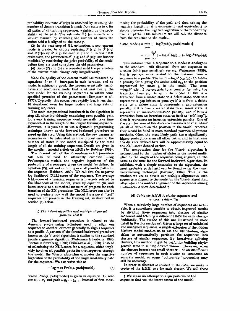
Figure 2. HMJI architecture for discovering sub- families.
components of the (composite) HYJI. Presently. the number IC of clusters and the initial lengths of the ~notlels €or these dustem are determined empirically. \Ye then add 8 new begin state with w outgoing transitions. one to each of the begin states of the component HWls (sre Fig. 2).
This new begin state is analogous to the other begin states in that it generates no amino acid. IVe then train this composite model with the El1 algorithm as c1eucril)ecl in section (b). above. The EM re-estimation of a co111- ponent model is the same as the reetimation of a sinplr model, except that the weight that a sequence has in the re-estimation of a component is proportional to the p r o b - ability of the sequence given that com1x)nent nwclel.
\ Thus, sequence that have better S L I ~ c o r e s for a parti- h l a r HMN component hare greater influence in re-(?;ti- mating the parameters of that component. and this ~ a u . w s t he parameters of that component to change in such a way that the component further *'specializes" in n~twleling those sequences. The "surgery" I)rowclurr clrscribetl belor in section (8) is used to adapt the length of that component to further specialize it. In this manner. the individual romponents evolve during training to wprrsrnt clusters in the training sequences. This way of using EN is called mixture modeling in the statistics literature (1)ucla gL Hart. 19f3: Ereritt Pr Hand. 1981). and is known as "(soft) competitive learning" in t h e neural nrtuork litera- ture (Sowlan. 1990).
When the model is trained. the probability of a sequence gi\-en any of the submodels van be ralruiatrtl. Le. the probability that the sequenc! belongs to the corresponding cluster/subclass. The negative logarithm o f this probability corresponds to the SI,1,-score calculatrcl for a simple HJI3I. As with the standard H W I we use. this yields a quantitative measure of how \vel1 the n~odel fits the data. The dusters found can also lw compare<l to
known subfamilies of the sequences. Esperimeots with the clustering of globin sequences are described in Results section (a).
(e) Modeling protein domains with an H l . t 1 There are many cases when one does not want to build
a statistical model of a family of whole proteins like globins, but instead to build a model of a structural motif or domain that oc*curs as a subsequence in many different kinds of proteins. such as the EF-hand motif (Kakayama et al., 1992) or the kinase catalytic domain (Hanks & Quinn, 1991). Here we expect. our model'to only match a relatively small subsequence of any given protein, wit.h many other unmatched amino acids appearing before and after this subsequence. One approach to this problem is to alter the dynamic programming method used to align a sequence to a model so that. it tries all possible ways of aligning each subseyuence of the sequence to a model (Waterman. 1989). lye use a simpler (but almost equiva- lent) method in which only the HMY model is altered. so that the same standard procedures (forward-backward ant1 Viterhi) \vhich we use for models of whole proteins can he used \rithout modification for modets of domains.
('onsider a training set of many unaligned sequences consisting not of complete proteins. but of a specific domain. Our tirst step is to train an HYM for these sequences esactly as described earlier. As shown in Figure I . this HNJi \vi11 h a w initial and final "dummy" match states m, and mN- I (where S + 1 = 5 in Fig. I ) that do not match any amino acid. To alter the HJIM to represent a protein domain. we cntrrte 2 new insert states i, and i,. adding i, to the n~odel before the state nlo and i, at the end of'the model after mNTI (see Fig. 3).
K P then acid a new clntnm_v BEOIS state before i, ant! a nrw duintny R S I ) state after i,. Eight new transitions are also atlclrtl to the IIIOCICI. The first 4 are from BEGTS t o i,. fronl m y -, to i,. and the self-loops from iB to itself and froln i, to itself: Thew all haw the same prohabi1it.y 1'. for sonw 1' lwtwwn 0 and I . The second 4 transitions are fron~ i, to m,. from I3E:CTS to m,. from i, to ESD. and from 111,~- t o KXD. Thme a11 haw probability I - p . The new states atltletl hrforr and after the modet. along with these transitions. form 2 new tnddules. 1 for matching the estra atnino acids that occur in the sequenc*..I)efi)re the hnain. and the other for matching the amino acids aftrr the clotnain.
The choice of the Imranleter p does affrct the way that the overall rnwlel aligns with a given q u e n c e . To see ho\v. it is conwnirnt to think of the negative logarithm of the prol)al)ility of a transition as a penalty for using that transition. as tlescrilwtl i n section (c). above. In the modi- tied n1cwlel. all sequences must suffer a penalty of -log ( I - p ) to enter and again to esit the domain part of the model. no matter which path they take. Hence this penalty is a tisrtl c w t . which ran fw ignored when
Figure 3. H U M architecture for modeling donlains.

comparing the distances or S L 1 ~ c o r . e ~ of 2 sequences with respect to the model. In addition to this penalty. all sequences will suffer a penalty of /i ( - l o g p + log 20). where K 2 0 is the number of amino acids that are not matched to the original domain model. but are instead matched in the states i, and i,. The -log 20 term arises because we set t.he probabilities of each amino arid to 1/20 in the insertion states i, and i, (see Krogh el nl.. 199.3~). Thus p wilt determine the "pressure" on the sequence to align something to the domain model. i.e. if 1) is low it is advantageous to squeeze many amino acids into the domain model. using the insert states in this part of the model. If it is high. it is possible that most sequences would prefer to pass through the delete states in the domain model. aligning ex-erything instead to t h e new modules before and after it. It is straightforward to estimate p the same way a s all the other paranwters. the only additional problem is that the rrilnw value nmst he used in all the transitions that 11.w this v a l w . -tying" these parameters to each other. Othrnvisc the model might become biased towards aligning the tlomain either near the beginning of the sequence or near the end of the sequence. We hare not attempted to estimate p. Rather. we have useda fixed p = 1 with goor1 results. (This should be thought of as a limit of p approad~ing 1. otherwise -log (1 - p ) is infinite.)
Using this construction. it may also he 1)ossible to discover interesting domains by training on whole protein sequences, and letting EM determine which part of the proteins to model. Furthermore. if more than one occur- rence of t.he same domain is expected in sonle sequences. then this model can be further modified to find all occur- rences. This is accomplished by simply adding a transition from the EXD state back to the.BE(;IS state.
(f) Searching a database wifh an H.11 SI Once an HMM is built for a family of proteins. it can be
used to search a database such as PIR or S\VISS-PROT for ot.her proteins in this family. Similarly. if an Hll l i is built for a protein domain or motif. then it can be used to search for occurrences of this domain or motif in the database. much like a PROSITE espresion (Rairoch. 1992). a commonly used method for searching for patterns found in protein sequences. Like a profile ( f a t e m a n (I: Perlwitz. 1986 Barton & Sternbeg. 1990: Gribskov el a/.. 1990: Bowie et ai.. 1991: Liithy et al.. 1991). an HJIJI has an advantage over a PROSITE expression for database searches. It takes into account a large amount of statis- tical information in matching a sequenw. and weighs this information appropriately. rather than relying on rela- tively rigid matching rules.
As described in section (b). above. the fonvard part of the forward-backward' dynamir programming method calculates a BLtscore for any test sequence that measures how well it fits t he model. This SLL-score is the negative logarithm of the probability of the sequence given the model. It turns out that this raw SLL-score is too dependent on the length of the test sequence to be used directly to decide if the sequence is in the family modeled by the HMIM or not. However. we can over- come this problem by normalizing this SLL-score appropriately.
Whenever we build an HMM for a family of proteins or for a protein domain. we run all the proteins in a standard database (for instance. SWISS-PROT) through this HMM and compute the SLL-score for each sequence. A scatter plot of sequence length r w w s SL1.-score for our kinase catalytic domain model is given in Figure 9.
Most proteins tend tn lie on a fairly straight line (towards the top of the plot) indicating that the SLL-score for these proteins is proportional to their lengths. These proteins are the ones that do not contain the kinase catalytic domain and thus look like "random proteins" to the kinase catalytic domain model. In contrast. the proteins that do contain the kinase catalvtic domain tend to have SLL-scores that are much lower than espected for. proteins of their length. and hence appear below the linear band of non-kinase proteins.
We can quantify the difference between SLL-scores for prot.eins containing the kinase catalytic domain and ST,I,-scores for proteins not containing the domain by a simple statistical method, as follows. Csing a local windowing technique.t we first calculate a smooth average curve for the roughly linear band of the SLL-score rer.ms length plot. The standard deviation around this average curve is also calculated. Using this. \vc. calculate the difference between the SLL-score of a sequence and the average SLGscore of typical sequences of that ~ ~ n e length. measured in standard deviations. This number. is called t.he 2-score for the sequence. We then rhoow a 2-score rut-off. either [I priori or by looking at the histogram of 2-scores for sequences in t.he database (see Fig. I O ) . and use it to decide if a given sequence fits the model or not. We have found that a 2-score of approsimately .i appears a good choice in most cases we hare esaminrtl. but we suggest carefully checking the '
histogram by eye before deriding on a cut-off. For esample. for our HMM of the kinase catalytic domain. sequences with 2-scores below 5 are classified as not 'c-ontaining the kinase catalytic domain, and sequences with 2-scores above 5 are classified as containing $e catalytic domain. If the 2-score of a sequence indica& that it contains the catalytic domain. we can align the sequence to the catalytic domain HMlI to find out where this domain occurs in the sequence. The time it takes to do a database search is proportional to the number of residues in the database times the length of the model. For our globin model (length 145) we can search the WISM-PROT database (about 8.375.000 residues) in approsimately 2 CPZ: hours on a Sun Sparcstat.ion 1. I'sing the shorter EF-hand model (length 29) it takes only 18 C'PV .seconds (1 1 user min) on a Sun Sparcstation 2. X parallel implementation of the search procedure (not r e t implemented) r i l l speed up these searches substantially, as it has the EM training procedure.
While the statistical techniques we have used to deter- mine 2-scores are still quite crude. we hare found that the HYJIs are sufficiently good models that these techniques work \vel1 enough in practice. However. i t may be that more sophisticated techniques are needed in certain cases.
t The arerage curve is calculated a s follows. For each length i starting at i = 1. the length I , is computed such that there are at least 500 proteins of lengths i to li and less than 5013 proteins of lengths i to I, - 1. The length interval i to li is called a window. The average curve is piecewise linear through the points corresponding to the average length and average XU-score for each window. The first and last parts of the curve are calculated by linear regression in the first and las t window. respeetirely. The standard deviat.ion of t.he points from the smooth curve is also calculated for earh window. The estimate of t.he average run.e can he impmwd by eliminating outliers. i.e. XLT.-scores that lie many standard deviations from the average. W e iterate the p r o w s of removing outliers and re-estimating the average curve until no more outliers remain.

(g) Initial d e l , i d minima, and choice of model length As mentioned in section (b), above, when estimating
the model from the training sequences, the EM algorithm does not guarantee convergence to the best model. It is basically a steepestdescent-type algorithm that climbs the nearest peak (local maximum) of the likelihood func- tion (or the posterior probability in MAP estimation). Since finding the globally optimal model seems to be a difficult optimization problem in general (Abe & Warmuth, 1990), we have experimented with various heuristic methods to improve the performance of the method.
Probably the best method is to give the model a hint if something is already known about the sequences, which is often the case. A good starting point makes it much more likely that the nearest peak is at least close to optimal. This is done by setting the probabilities in the initial rnodei to values reflecting that knowledge. If, for instance, an a l i m e n t of some of the sequences is available, i t is straightforward to translate that into a model by simply cnlcuIating the relative frequency of the amino acids and the transition frequencies in each position, as in the profile method (Gribskov et al., 1990).
It is of course even more interesting if the model can be found from a M a ‘ma, i.e. using no knowledge about the sequences. For that we have used an initial model where all equivalent probabilities are the same, i.e. d ( q + l I m k ) is independent of the position k in the model, and similarly for all other transition probabilities, and 9(zlmk) is also independent of k. To avoid the smaller local maxima. noise is added to the model during the iteration before each re-estimation. Initially quite a lot of noise is added, but over 10 iterations the noise is
\decreased linearly to zero. Since noise is added directly to ‘$he model, it is not like the usual implementation of iimulated annealing, but the principle is the same. The “annealing schedule” is p&ntly rather arbitrary, but it does seem to give reasonable resultsf if it is applied several times, and the best of the models found is used as the final model.
It is important that the best model be selected, since suboptimal models do produce inferior alignments in general. However, when studying alignments from sub- optimal globin models, we noted that they tend to align some regions well. occasionally getting better alignments in those regions than the best overall model found, while in other regions they are completely incorrect. This leaves open the intriguing possibility of combining the best solutions found for diRerent regions into a new overall best model. We have not yet explored this possibility.
The length of the model is also a crucial parameter that needs to be chosen a priori. However, we have developed a simpie heuristic that selects a good model length, and even helps in the problem of local maxima. The heuristic is this: after learning, if more than a fraction$ ydel of the paths of the sequences choose dk, the delete state at position E , that position is removed from the model. Similarly, if more than a fraction yinr make insertions at. position k (in state it), a number of new positions equal to the average number of insertionwmade at that position are inserted into the model after position k. After these
t An alternate method that also appears to give good results has been developed by Baldi el al. (Baldi el al.. 1993: Baldi & Chauvin, 1993). This method uses stochastic gradient descent in place of the EM method, which may help in avoiding local minima.
1 Currently we choose yde, and yinr each to be 1/2.
changes in the model, i t is retrained, and this cycle is repeated until no more changes are needed. We call this “model surgery”.
(h) Over-@ing and H A P mtimatia A model with too many free parameten cannot
estimated well from a relatively small data set of training sequences. If we try to estimate such a model, we run into the problem of overfitting, in which the model fib the training sequences very weI1, but gives a poor fit to related (test) sequences that were not included in the training set. We say that the model does not “generali~” well to test sequences. This phenomenon has been .well documented in statistics and machine learning (see e.g. Geman el al., 1992; Berger,.1985). One way to deal with this problem is to control the effective number of free parameters in the model by using prior information. This can be accomplished with MAP estimation. Parametem that we assume (via our prior distribution on models) ~ 8 n
be wellestimated a priori in effect become l e s s adaptive, because.it takes a lot of data to override OUF prior beliefs about them, whereas those about which we have only weak prior knowledge are estimated in almost the same manner as in maximum likelihood estimation. In this way. the model can have a very large number of para. meters, but a much smalier number of “effectively free” parameters. To make MAP estimation practical, we use Dirichlet distributions as priors. The details of the method are described elsewhere (Krogh et al., 1993a; Brown d d., 1993).
3. Results (a) Globin experiments
The modeling was first tested on the globins, a large family of heme-containing proteins involved in the storage and transport of oxygen that have different oligomeric states and overall architecture (for a review see Dickerson & Geis (1983)). Hemoglobins are tetramers composed of two OL
chains and two other subunits (usually B, y , d or 8). Myoglobin is a single chain, some insect. globins are present as dimers and some intracellular inverte- brate globins occur in large complexes of many subunits.
Globin sequences were extracted from the SWISS-PROT database (release 19) by searching for the keyword “globin”. Eliminating the false positives. resulted in 625 genuine globin sequences of average length 145 amino acids. We left three non-globins in the sample for illustrational purposes giving a total of 628 sequences. The sample of globins in the database is not the random sample a statistician would prefer, but is perhaps one of the best and largest collections of protein sequences from a homologous family. Sesrching for the words “alpha“, “beta”, L‘gamma’’, “delta”, “theta”, and “myoglobin” in the data file yielded 224 alpha, 199 beta, 16 gamma, 8 delta and 5 theta chains and 79 myoglobins, which adds up to 531 sequences. These should naturally be considered minimum numbers. but they give a good picture of how skewed the sample is.
To t e s t our method, we trained an HMM using the method described in Methods sections (b) and

H zdden ill arkoa 111 odels 1 DUY
Helix AAAAAAAAAAAAAAAA BBBBBBBBBBBBBBBBCCCCCCCCCCC DDDDDDDEE HBA-HUNAN --------- V L S P A D K T N V K A A W G K V G A - - H A G E Y G A E A ~ ~ F ~ F P T - - - - - BGSA HBB-HUNAH -------- VHLTPEEKSAVTALWGKV----NVDEVGGEALGRLLWYPWTqRFF~FGD~TPDAVHGNP MYG-PHYCA --------- VLSEGEWqLVLHVWAKVEA--DVAGHGqDILIRLFKSHPE~~FD~H~~AEHKASE GLB3-CHITP ---------- LSADQISTVqASFDKVXG------ DPVGILYAVFKADPS1HP;K.FTQFAG-KDLESIKGTA GLB5,PETMA PIVD'PGSVAPLSAAEK?XIRSAUAPVYS--nETSGVDILVK~STPAAqE~PK~GL~ADQLKKSA LGB2-LUPLU -------- GALTESqAALVKSSWEEFNA--NIPKHTBRFFILVLEIAPAAKDLFS-nK-GTSEVPqNNP GLBI-GLYDI --------- GLSAAQRqVIAATWKDIAGADNGAGVGKDCLIKFLSAHP~HAAYFG-FSG----AS---DP
Helix EEEEEEEEEEEEEEEEEEE FFFFFFFFFFFF FFGGGGGGGGGGGGGGGGGGG HBA-BUNAB QVI(GBGKKVADALTNAVAHV---D--D#PNALSALSDLHAHKL--RVDP~YFKUSBCUVTLAAELP~ HBB-BUMAH K~AH~KKVLGAFSDGLAHL---D--NLKGTFATLSELHCDKL--HVDPEHFRLLGBVLVCV~AEEFGKE
' HYG-PHYCA DLKKBGVmLTALGAILKK----K-GHHEA~P~qSHATKH--KIP~~~IS~II~VLHS~~PGD GLB3,CHITP PFETBANRIVGFFSKIIGEL--P---NIEADVNrrVASHKPRG---VTHDq~N~~AGFVS~HT--D GLB5,PETMA DVRWBAERIINAVNDAVASM--DDTMHSIIKLRDLSGKHAKSF--q~P~~~AVI~TV~G---- LGB2,LUPLU ELqAaAGmr~LVYEAAIqLQVTGVWTDATLKNLGSVHVSKG---VAD~P~EAILKTIK~VVG~ GLBI-GLYDI GVAALGAKVLAqIGVAVSHL--GDEGKllVAqHKAVGVRHKGYGNKHIKAQYFEPLGASLLSAHEHRIGGK
Helix HHHHHHHHHHHHHHHHHHHHHHHHHH HEI-EUKAI FTPAV3ASLDKFLASVSTVLTSKYR------
' BBB-HUZIAB FTPPVqAAYQKWAGVANALAHKYH------ HYG-PHYCA FGADAQGAHHKALELFRKDIAAKYKELGYQG GLB3,CHITP FA-GAEAAUGATLDTFFGHIFSKM------- GLB5,PETMA ----- DAGFEKLnSHICILLRSAY------- LGBZLUPLU WSEELlDSAVTIAYDELAIVIKKEMNDAA--- CUI-GLYDI MUAAAKDAUAAAYADISGALISGLQS-----
\ Figure 4. Seven representative globin sequences of known structure and their alignment taken fmm Bashford et a.S,
(1987). The letters A to H in Helix denote the 8 different a-helices. Some regions, especially CD, D and FG, are not well defined. The sequences and their SWISS-PROT identifiers are Human a (HBA-HUMAK), human fl (HBB-HUMAN), sperm whale myoglobin (MYGSHYCA), larval Chir0nomou.s thvmmi globin (GLB3-CHITP). sea lamprey globin (GLWETMA), Lupinus Z u & m leghemoglobin (LGBLLUPLV): and bloodworm globin (GLBLGLYDI). (In SWISS-PROT 19 a S is used instead of an ''-" in the identifiers.)
(gf. We used a homogeneous initial model that contained no knowledge about the globin family. Its probability parameters were derived from the prior, and were the same for all equivalent transitions (i.e. 9 different transition probabilities). All amino acid probabilities (the B distributions) were set equal to the distribution of the amino acids given by Krogh et d. (1993a). In the insert states we used a prob- ability of 1/20 for all amino acids. The only model parameters set by hand are the initial transition probabilities and corresponding regularization para- meters (see Krogh et d., 1993~). From our experi- ence, the method does not seem to be very sensitive to the choice of these parameters, but i t would require considerable further experimentation to verify this quantitatively. For our training set, we picked 400 sequences at
random from the 628 sequences. We withheld the remaining 228 sequences in order to test the model on data not used in the training process The model was trained using noise and model surgery (ysrr = y h = 05), as described in Methods section (g). This procedure was repeated about 20 times with model lengths chosen randody between 145 and 170. The average run-time was around 60 CPU minutes on a Sun Sparcstation I. For each run we computed a
XLL-score for the model, which was the average of the ELL-scores for the training sequences, as defined in Methods section (b). The final NLL-scores varied considerably for these runs but the best was 210.7.
We then took this model, produced ten new models by adding noise, and optimized these. These models all generated approximately the same NLL-score and we picked the model with the best NLL-score, 2103, having a length of 147. W e vali- dated this modelt in two ways: from the alignments it produced, and by its ability to discriminate between globins and non-globins. The results are described below.
(i) Multiple sequence a l ~ m e n t s A multiple alignment of many globin sequences has been produced by Bashford et d. (1987) by including into the alignment procedure tertiary- structure information of seven globins (Fig. 4). This
t We stress t h a t the final model was chosen according to an objective measure, namely the KLL-score on the training set. and not retroactively on the basis of how well it did in multiple alignment or database search tasks.

1610 Hidden Markov Modds
was achieved by aligning these seven sequences and then aligning the rest of the 226 studied to the closest of these seven. In contrast. generating multiple alignments with HMMs requires no prior kno.rvledge of underlying structure. Using the globin HM3fCI, we produced a multiple alignment of all the 625 globin sequences by the Viterbi algorithm as described in Methods section (c). Figure 5 shows this alignment for the seven sequences from Bashford et a l . (198i).
The alignment found in ,this experiment agrees estremely well with the structurally derived align- ment of Bashford et al. Our alignment differs in the region between the C and E helices. However, this is a highly variable area since only some globins possess a D helix. The difference in the F/C-helices is mare pronounced. with the remaining discrepan- cies possibly representing an alternative alignment. Four of the insertions the model chose are in vari- able regions between or at the end of helices. i.e.
Helix AAAAAAAAAAAAAAAA ***************+
between secondary structure elements, The 1s t two insertions appear in the F/G region.
(ii) Database search.: discriminating globins f.Om
The globin HMM model we found was also tested on ail t.he 25.044 proteins in the SWISS-PROT data- base release 22-0 of length less than So00 amino acids (which is all but 2). A XLL-score and a 2-score were computed for each of these sequences as described in Methods section ( f ) . These are plotted in Figures 6 and 7 as a scatter plot and a histogram, respectively. For the histogram (but not the scatter plot), the data were filtered as follows:
All sequences with a 2-score >3.5 and either more than a total of 23, or more than IS*/, unknown residues were removed (a total of 23). Currently, we treat an unknown a.mino acid, X, as being the most probable amino acid at the position it is matched to,
non-globins
BBBBBBBBBBBBBBBBCCCCCCCCCCC DDDDDDDEE ++++++++****************++* +
HBA-HUHAN V.........LSPADKTNVKAAWGKVGA..HAGEYGAEALERHFLSFPTTKTYFPHF-DLSHGSAQ---- HBB-BUXAN Vh........ LTPEEKSAVTALWGKV--..MmEVGGEALGRLLWYPWTQRFFESFCDLSTPDAVMGNP MYG-PHYCA V.........LSEGEWQLVLAVWAKVEA..DVAGHGqDILIRLFKSBP€TLEKFDRFKHLKTEA€~ASE GLBI-CHITP -.......... LSADqISmQASFDKV--..KGDPVG--ILYAVFKADPSIMAK~~-AGKDLESIKGTA GLBS-PETMA PivdtgsvapLSAAEKTKIRSAUAPWS..TYETSCVDItVKFfiSTPAAQ€~~PKFKGLTTADqLKKSA LGB2,LUPLU Ga ........ LTESQAALVKSSWEEFNA..NIPKHTHRFFILVLEIAPAdKDLF-SFLKCTSEVPq-NNP
\ GLBI-GLYDI G. . . . . . . . .LSAAq~VIAATWKDIAGadNCAGVGKDCLIKFLSAHP~MAAVF-GF----SGASD--'P '\.
Helix EEEEEEEEEEEEEEEEEEE FFFFFFFFF FFFFFGGG GGCGGGGGGGGGGGGG +****************** ********* ***************+
HBA-IIUHAI -VKGHGKKVADALTNAVAHVDD.....HPIALSALSDLHA...HKLRVDPV.NFKLLSHCLLVTLAAHLP HBB-EUHAN KVKAHGKKVLGAFSDGLAHLN. . . .. LKGTFATLSELHC ... DKLHVDPE.NFRLLGN~VCVLABHFG WG-PEYCA DLKKHGtlTVLTALGAILKKKGH ..... HEAELKPLAQSHA ... TK-HKIPILYLEFISEAIIHVLHSRRP GLB3-CHITP PFETHAPRIVGFFSKIIGELPN . . . . . IEADVNTFVASHK. . . PR-GVTHD. QLHIFRAGFVSYMKAH-- GLB5-PETHA DVRWHAERIIIAVNDAVAS~Dtek .. HSXKLRDLSGKHA ... KSFqVDPq.YFKVLAAVIADTVAA--- LGBP-LUPLU ELPAHACKVFKLVYEAAIQLQVtgvvvTDATLKHLGSVKV ... SK-GVADA.HFPWKEAILKTIKEVVG GLBI-GLYDI GVAALGAKVLAQIGVAVSHLGDegk..MVAqPIXAVGVRHKgygNK-HIKAq.YFEPLGASLLSAMEHRIG
Helix HHHHHHHHHHHHBHHHBAHHHHHHHH ++**+******************
HBA-BUHAN AEFTPAVHASLDKFLASVSTTLTSKY ...... R HYG-PHYCA GDFGADAQGIMlKALELFRKDIAAKYkelgyqG GLB3,CHITP TDF-AGAEAAWGATLDTFFGMIFSKH ...... - GLB5-PETHA GD------ AGFEKLMSMICILLRSAY. ..... - LGB2,LUPLU AKWSEELRSAWTIAYDELAIVIKKEMnda ... A GLB1,CLYDI GKHNAAAKDAWAAAYADISGALISGLq ..... S
F- HB3,HLJHAN KEFTPPVQAAYQKVVAGVANALAHKY ...... H
Figure 5. The alignment Of the same 5 globins as in Fig. 4. as obtained from our model trained on 400 randomly chosen globin sequences. The capit.al letters represent amino acids aligned to the main line of the Inoclel. -. to deletions in the model. and lower-case letters to amino acids treated as insertions by the model. The . is used as a fill character to accommodate insertions. So attempt has been made to align the insertion regions. Tn the line above the alignments * indicates complete agreement of a column ivith the structural alignment (Fig. 4) and + denotes a minor deviation (the only accepted difference is a reasonable displacwnent of a gap). The regions between the helires are not checked in this way. The training set contained 5 of the 5 globins. not HBX-HUMAS and GLRLPETMA.

l 1 . , , I , ( . . , 100 200
Length of Sequence
Figure 6. Plot of SLL-SCOW. wr.wx sequentv length for globins an? non-globins. . . M I sequences of length less than 300 from the S\YISR-PROT P i database are sho\va. including partial sequences and 3 false globins from the globin file. and sequences from the database containing man?- Ss. \
300
E3 non-globins training set I test set
3000 10 e 6
4 2 0
Z-score Figure 7. Histogram showing the number of sequences
with a certain 2-score. The training set of 397 globins. the test set of 231 globins. and the rest of the sequences from SWTS+”-PROT P2 after “filtering” are shown. The insert shows expansion of the region around a Z-score of 6.
so sequences with many lis spuriousi~ match the model very well.
Since we searched a newer release of SWISS-PROT (release 22) than the one from which the globin training set was extmcted (release 19), eight new globins were found and incorporated into the test set.
Five globin fragments of length 19 to 45 were removed from t.he data.
Three non-globin sequences in the globin file that were identified as outliers in Figure 6 were removed. One of these non-globins was left as part of the training set to illustrate the robustness of the method.
The model distinguishes extremely well between globins and non-globins. Choosing a 2-score cutoff of 5 we would miss 2 out of 628 globinst and get essential]? no false positive globins. There is one ”non-globin”, a bacterial hemoglobin-like protein (SWISS-PROT id HMP-ECOLI)l that may or may not be- counted as a false positive. Only one sequence, the heme containing catalase of Penicillium vilale (CATA-PENVI, Z-score C7), has a Z-score between 4.2 and 5-1, so any cutoff in this range will essentially give the same separation. The two sequences falling between a. Z-score of 1. and 4
t 628 in the original data set. plus 8 new. minus 3 spurious. minus b fragments. 39i were left from the training and the remaining 231 made up the test set.

1512 Hidden Markov Models
(GLB-PARCA and GLB-TETPY) are protozoan, whereas the other globins are metazoan. The primary sequences of these globins are similar and have little similarity with other eukaryotic globins. Note also that both of these sequences are in the test set.
(iii) D i m e r i n g subfamilies of globins We also performed an experiment to automatically discover subfamilies of globins using the method described in Methods section (d). An HMM with ten component HMMs was used. The initial lengths of the components were chosen randomly between 120 and 170, but were adjusted by model surgery during training. We trained this HMM on all 628 globins and then calculated the NLL-score for each sequence for each of the ten component HMMs. A sequence was classified as belonging to the cluster represented by the component HMM that, gave the lowest KLL-score, i.e. the one giving the highest probability to that sequence.? Three of these clusters were empty and the remaining seven non- empty ones represented chains from known globin subfamilies:
C b s X. 233 sequences: principally all CY, a few [ (an a-type chain of mammalian embryanic hemo- globin), %/x' (the counterpart of the a chain in major early embryonic hemoglobin P), and 8-1 chains (early erythrocyte a-like).
Class 2. 232 sequences, almost all a few 6 \(p-like), E (&type found in early embryos), y (comprise fetal hemoglobin F in combination with 2 Or chains), p (major early embryonic /.?-type chain) and 6 chains (embryonic &type chain).
C b s 3. 'il myoglobins. C h s 4. 58 sequences. The 13 highest scoring in
this cluster are leghemoglobins. This class contains a . variety of sequences including the three non-globins
in original data set. Class 5. 19 sequences. Midge globins. Class 6. Eight sequences. Globins from agnatha
Class 7. Seven sequences. Varied. We have not repeated this experiment using
different randomization to ascertain if better results can be obtained. However, we are encouraged by the results of this first experiment since it is able to classify correctly t h e major globin subfamilies (alpha, beta and myoglobin).
(iv) The $rial globin model Examination of the model itself yields information on the structure of globins. Figure 8 shows the normalized frequency counts (the numbers used to re-estimate the parameters of the model) from some parts of the final model. The thickness of a line
(jawless fish).
~~
7 We can also calculate the posterior probability of each cluster by looking at the transition probabilities out of the global start state, and thereby obtaining a posterior distribution over the 10 clusters for each sequence. However, these posteriors are very sharply peaked, so this adds little to the analysis.
indicates what fraction of the 400 training sequences made that transition or used that padi- cular amino acid. A broken line indicates that less than 5% of the sequences used that transition. (The continued delete is mostly due to fragments that have to make many deletions.) The histogram in a match state shows the distribution of amino acids that were matched to that state. The number in a n insert shows the average length of an insertion beginning at that position.
For the amino acids the ordering proposed by Taylor (1986) is used. S i r t i ng from the top, the amino acids are medium-sized and non-polar, small and medium polar (around G and P), medium sized and polar (around K), large medium-polar (around F and Y): and finally below they are medium-large and non-polar. There does seem to be some ten- dency for t.he distributions to peak around neigh- boring amino acids when using t.his ordering,.as one would expect. When one looks at the whole model, regions that are highly conserved are also readily distinguished from the more variable regions, both as a function of the probability that. a position is skipped, and the entropy of the distribution of amino acids at that position.
(b) Kinase experiments Protein kinases are defined as enzymes that
transfer a phosphate group from a phosphate donor onto an acceptor amino acid in a substrate protein (Hunter, 1991; Hanks et d., 1988). Based upon the accept.or amino acid specificity, they have been classified into serine/threonine, tyrosine, histidine, cysteine, aspartyl and glutamyl kinases. Only enzymes in the first two categories have been well characterized and recent deyelopments indicate that some can phosphorylate both a.lcoho1 (serine/ threonine) and phenol (tyrosine) groups, the so- called dual-specificity protein kinases (Lindbmg et a.1.: 1992). It. is the region comprising the catalytic domain of these hydroxyamino acid phosphory- lating enzymes t.hat we model by an HMM and which we subsequently refer to as protein kinases or simply kinases. Despite the differences in size, substmte specificity. mechanism of activation, sub- unit composition a.nd subcellular localization: all these kinases share a homologous catalytic core c,ontaining 12 conserved subdomains or regions (Hanks 8; Quinn, 1991; Hanks et al., 1988).
Because the kinase catalytic domain is only a subsequence embedded in a Iarger protein, the kinase experiments differed from the globin experi- ments. The HMM used in the globin experiments modeled t.he entire protein rather than simply a segment of a protein as is the case for the kinase family. Modeling domains requires several modifica- tions to our standard HMM training which are described in Methods section (e).
The training set. for these experiments is a group of 193 sequences from the March 1992 release of the protein kinase catalytic domain database main- t.ained by Hanks & Quinn (1991). This set is

Hidden Markov Models 1513
Figure 8. Parts of the final globin model. The position numbers are shown in the delete states.
composed of serine/threonine, tyrosine and dual- specificity kinases principally from vertebrates and higher eukaryotes but also includes some from lower eukaryotes and viruses.
We trained ten HMMs on all 193 (unaligned) ' sequences in this- data. set using the prior distribu-
tions described by Krogh et ul. (1993~). N o para- meters. of the modeling process were set manually and the initiaI model lengths ranged from 242 to 282 positions (this encompasses the average length of the sequences in our kinase catalytic domain training set). At the end of the ten training runs, the best kinase model had a NLL-score (the average --logP(sequenceImodel) over the training set) of 588.39 and a length of 254. Modules were added at the beginning and end of this model as described in Methods section (e). We tested this model in the same manner as described earlier for the globin model.
Our main tests were discrimhation tests, in which we utilized the model. to search the SWISS-PR.OT version 22 database (25,044 sequences) for proteins containing the kinase catalyt.ic domain.
As described in Methods section ( f ) , a NLL-score was computed for each of the sequences in the database and this information was used to compute a sequence's deviation from the average curve as measured by a Z-score. The data were then filtered to remove all sequences with any unknown residues (353) and all sequences having length less than 200 (4230): since complete protein kinase catalytic domains range from 250 to 300 residues (Hanks et al., 1988). This filtering removed a total of 4386 sequences. A scatter plot of NLGscore vemw length for the SWISS-PROT sequences is given in Figure 9.
A cutoff of 6-0 was chosen because there are no sequences with Z-scores between 4935 and 6773. See Figure 10 for a histogram of the resulting Z-scores. Any sequence having a Z-score >6.0 was therefore classified as containing the kinase cata.- lytic domain while those with Z-score t6.0 were classified as not possessing the domain. With this cutoff, 296 sequences were classified as containing the kinase cat.alytir domain. The remaining 20,357 srquerx-w \\-ere rejecttd.

1514 Hidden Yarkoa Models
t , Certain Kinases
. Rest of SWISS-PROT
Figure 9.
~ ~ ' " ' ' ' " " " ' ' " ' t 500 1000 1500 2000 Length of Sequence
scatter plot of SLL-score \-ersus length for sequences in SiVISS-I'ROT using the Kinase HMX
', The genera.1 issue of estimating the number of false negatives and false positives when distinguishing sequences belonging to a given family
I Certain Kinases
a All other sequen- ces in SWISS-PROT
* . .
C l O 0 10 20 30 40 ! Z-score
Figure 10. Histogram showing the number of sequences with H certain %-score relative to the kinase model.
from non-members is a complex one. In the case of 'the glohins. it is "relatively" straightforward since it 4s possible to identify all the globins in t.he data- base l ) ~ prfonning a keyword or title string search. The situation for the kinase domain or the EF-hand motif (see section (c) below) is less obvious and thus more problematic. For instance, while a given pro- tein may possess the' sequence characteristics for this motif or domain. functionally, the region may not bind calcium or possess kinase activity. We hare attempted to address this complicated matter as best we can as described below. However, we stress that ~r -e do not feel able to give a definitive answer as to the number of true false negatives and true false positives in our kinase or EF-hand data- base discrimination test.s.
A list of potential protein kinases was created from the union of sequences designated as being kinases from four independent sources: our HMM, PR.OSTTE (a dictionary of sites and patterns in proteins (Hairoch. 1992)), PROFTLESEARCH (a technique used to search for relationships between a protein sequence and multiply aligned sequences (Gribskor et ai., 1990)) and a. keyword search.
Two regions of the catalytic domain of eukaryotic protein kinases have been used t,o build PROSITE signature patterns. The first pattern corresponds to an area believed to be involved in ATP binding (PROSTTE: entry PROTEIXKIXASEATP, sequence motif [ l,I\-]G.C.tF~~lJ[Sc].\'). There are two signature patterns for the second region impor- tant for ratalytic activity: one specific for serine/

Hidden Markov Models 1515
threonine kinases (PROTEIS-KTSASE-ST, ILIV~~FYC].[HY?.D[LIV,MFT]~.PS[LIV.MFYC]I) and the other for tyrosine kinases (PROTEIS- KIPU'ASE-TTR, [LIV~F~C}.[HY].D[L~~~lF~J [RSTA].ZX[LIVXFYCJB). Since PROSJTE expressions do not albw for flexible gapping or insertions, a profile of k i n a was constructed from an alignment of seven kinases and employed for database discrimination tests (11. Gribskov, persona1 communication) using the program PROFILESEARCH (Gribskov rt ul.. 1990). The seven kinases used to generate the protile ;UT. bovine cA3rIP-rlependent protchin kinast. (I'IR wdc
OK BOG). bovine cGMP-dependent protein kinase (OKB02C'). bovine protein kinase C (KIBOC), human mos kinase-related transforming protein (TVHVFG): human re fa kinase-related trans- forming protein (TVHK"), mouse pim-I kinase- related transforming protein (WMSPI), and human feslfps kinase-related transforming protein (TVHVFF). The keyword search consisted of sea.rching t.he descriptions of the sequences in SWISS-PR,OT for the following strings: "SERISE/ THHEOSTSF:-PROTETS KTXASE. SER.;THR- T'ROTEJS KTXXSR. PR.OTElS-S;ERTSE/ 'I'HHEOSISI.: I<TS.WI<. PHOTk:TS-SER.,WHR

1516 Hidden Markov M.odels
KINASE, . TYROSINE-PROTEIN KINASE, TYR-PROTEIN KINASE, PROTEIX- TYROSINE KINASE, PROTEIN-TYR KINASE, V-ABL, C-ABL, V-FGR, C-FGR, V-FMS, C-FMS, V-FPS/FES, 1’-FES/F’PS, C-FPSFES, C-FESFPS, V-FYN, C-FYN, V-KIT. C-KIT, V-ROS, C-ROS, V-SEA, C-SEA, V-SRC,. C-SRC, V-YES, C-YES,, V-ERBB”. Of the 296 SWISS-PROT 22 sequences that were
above the Z-score cutoff of 6.0 and were thus classi- fied as containing a kinase domain b y our HMM, 278 were similarly classified by PROSITE, PRO- FILESEARCH and the keyword search. These 278
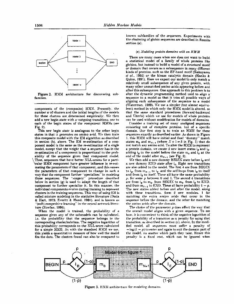
sequences may be considered to constitute “certain kinases”. Figure 11 shows the multiple sequence alignment generated by our HMM of some represen- tative kinases from this set (sequences 1 to 22). Sequences 23 to 40 are the 18 sequences (296 minus 278) that were designated as kinases by the HMM and one or two of the three other methods. For PROSITE, we consider a sequence to be a kinase if it satisfies one or more of the three patterns PROTEIS-KINASE-ATP, PROTEIN-KINASE- ST or PR.OTEIN,KINASE-TY R as a true positive (“T” in Fig. 11B). PROSITE false negatives (“N”), potential hits (“P”) and false positives (“F”,
Hidden Markov Models 1517
sequences which do not belong to the set under consideration) are ignored.
Among the 18 sequences classified as kinases by our HMM, eight (23 to 26, 35, 38 to 40) were also deemed to be kinases by the keyword search and PROSITE, and one (27) by PROFILESEARCH and PROSITE. The remainder (28 to 34, 36 to 37, those indicated by yo in Fig. 11 B) are particulate guanylyl cyclases and except for 36 to 3 i , PROFILESEARCH also defines them as possessing a kinase domain. These guanylyl cyclases contain a single transmembrane domain, a cyclase catalytic domain and an i n t r a r ~ l l ~ ~ l a r protein kinase-like
domain in which protein kinase activity has not been seen to date (reviewed by Garbers, 1992). Although these sequences are not kinases in terms of function, they possess all the conserved subdomains (subdomain I, the nucleotide binding'loop is modi- fied in some) and the majority of conserved residues present in certain kinases (see Subdomain of Fig. 11 A and positions indicated by *).
Sequences 41 to 50 are the top ten sequences in SWISS-PROT immediately below our cutoff of 60. Of these, the first three (41 to 43) were classified as kinases by two out of PROSITE, PROFILE- SE.4R.CH and the keyword search. Our cutoff was

chosen from a visual inspection of a histogram of Z-scores which indicated that 60 lay in a large gap (see Fig. IO). If the 2-score cutoff is lowered to the next largest gap (from 2-score 3.9 to 4-8) between sequences 43 to 44, then these t h r e e viral sequences (41 to 43) would also be categorized as kinases by the HMM.
Of the eight sequences (41, 51 to 53, 56 to 57. 59 to 6 0 ) that were not classified as kinases by our HMM but were classified only by the keyword search and PROSITE, one (41) is the first sequence below OUT cutoff discussed above. Four (56 to 57, 59 to 60) are partial sequences where the kinase
domain is ahsent. Three (51 t o 63) possess divergent forms of many of the cvnserred regions and like SI to 43. although they are below our cutoff, the HJIM is able to generate an alignment that correctly iden- tifies divergent forms of conserved regions. FinaIly, there are three aminoglycoside 3'-phosphatrans- ferase sequences (5.4 to 55,58) which are only desig- nated as kinases berause they sat.isfy the PROSTTE espression for the catalytic loop.
Inspection 0f'Figur.e 1 1 B permits an estimation of the accuracy of the various methods in dis- tinguishing kinases from non-kinases in database discrimination tests. The HMM generates six false

Hidden Markoa Models 1519
negat.ives (41 to 43,51 to 53) of which the first three fall immediately below our kinase cutoff. For PROFILESEARCH, there are 12 false negatives (23 to 26, 35, 38 t o 41, 51 to 33) but it should be recs l led that eight of these (those indicated by $ in Fig. 11B) do not appear in the results obtained from searching SWTSS-PROT 25 provided to us bx W. Gribskov (personal communication). 1Ve suspect that at least four (23 to 26) would be correctly classified as kinases by PROFTLEFEARCH leaving an estimate of three to eight false negatives. In the case of PR.OSTTE, using 0111- assumption of it kinast3 to be a true positive (T) s q w n w I i w m y t i l ' I!W
three patterns, there are three false negatives (39,42 to 43). However, the 8ctua.l performance of t he PROSITE patterns t.hemselves is much worse; scans of SWISS-PROT 22 with each of the patterns PROTEIXKIXASE-ATP? PROTEI'?;- KISASLf5T and PROTEIKXISASE-TYR indi- vidually yield 40, 2 and 3 false negatives, respectively.
The difficulty in quantifying the precise number of false positives and false negatives produced by the database discrimination tests may be illustra.ted l y emlhyinp an dternutire mechanism for assvssil1c t h 11~1nkwr c)f false ntyativrs. i f sin1pIy

1520 Hidden Markov Models
Figure 11. A, Multipte sequence alignment generated by our kinase HMM of some of the sequences used to train the HMM (1 to 22) and test sequences from the SWISS-PR.OT 22 database (23 to 60) (see Results section (b)). Pu'umerals appearing in the alignments indicate the number of amino acids to be inserted at that point. otherwise the notation follows the convention of Fig. 5. I n Subdomain, the Roman numerals and * refer to the subdomains and residues conserved across 75 serine/threonine kinases given by Hanks b- Quinn (1991). A and B in PROSITE refer to the ATP binding and catalytic regions, respectively, used to create 2 different signature patterns for kinases. X-ray identifies the location of the mhelices AA-AI and /3-strands Bl-B9 (read vertically) derived from the 2-7 d crystal structure of the catalytic subunit of cAMP-dependent protein kinase (sequence 1) (Knighton d a/.. 1991). Sequences 1 to 22 are representative kinases taken from the March 1992 Protein Kinase Catalytic Domain Database (Hanks & Quinn, 1991). These are: CAPIC-ALPHA, cAMPdependent protein kinase catalytic subunit. a-form: WEE1 +. reduced size at division mutant wild-type allele gene product; TTK, mouse serine/threonine kinase: SPKl . S. cerekier kinase cloned with anti-p- Tyr antibodies; RSKl-E, amino domain of type 1 ribosomal protein 66 kinase; PYT, putative serine/threonine kinase cioned with anti-p-Tyr antibodies; PKC-ALPHA, protein kinase C, z-form; PDGFR.-B. platelet-derived growth factor receptor B type; PBS2, polymix in B antibiotic resistance gene product: MIKl. S. pombe mikl aets redundantly with weel +; MCK1, S. cereviaiae protein kinase; 1XS.R. insulin receptor: HSI'K. Herpes simplex virus-US3 gene product; ERK1. rat irisulin-stimulated protein kinase; EGFR, epidermal growth factor receptor {cellular homolog of v-erbB); ECK, receptor-like tyrosine-kinase detected in epithelial cells; DPTKl . developmentally regulated tyrosine kinase in D. dkc.&ietLm; CLK. mouse serine/threonine/tyrosine kinase; CDC2HS. human functional homolog of yeast cdc2+/CDC28; CAMII-ALPHA. calcium/c&nodulindependent protein kinase 11. 1-subunit: C-SRC. cellular homolog of u-src; and C-RAF, cellular homolog of v-ruf/mil. Sequences 2 to 4.6. 10, 11, 14. 17 and 18 are t.he candidate dual-specificity protein kinases as defined by Lindberg et al. (1992). Sequences 23 to 40 are the SWISS-PROT 22 sequences designated as kinases by our HMM {Z-score >6.0) but not by all 3 other methods, PROSITE. PROFILESEARCH and the keyword search. Sequences 41 to 50 are the top 10 sequences below our cutoff of 6 0 and 41 to 13 and 51 to 60 are sequences that were not classified as kinases by the HMM but were so by one or more (but not all) of the 3 other methods. Kote that sequences identified as kinases by all 4 methods are not shown. All sequences that are less than 200 residues in length

Hidden Markov Models 1521
the number of sequences denoted as kinases only by all three other methods is evaluated, the number of false negatives for each of the techniques differ from the more detailed analysis: two .for .the HMM (42 to 43), seven for PROFILESEARCH (23 to 26, 35,38,40) and none for PROSITE (ignoring known false negatives as above). This general problem is further highlighted by the guanylyl cyclases (indicated by yo in Fig. I 1 B}. If the definition of a kinase is based upon function and not possession of particular sequence patterns, then the guanylyl cyclases are the only false positives for both the HMM and PROFILESEARCH. The PR.OSITE patterns PROTEINXINASEATP, PROTEI?;- KINASEAT and PROTEIN-KISASE-TYR produce eight, none and two false positires, respec- tively, giving some indication of the act.ual PROSITE performance.
OveraIl, both the HMM and PROFILESEARCH appear to perform generally better than PROSITE in the discrimination tests, with the HNM possibly having a slight advantage over PR.OFILE- SEARCH.
The HMM database search did not suggest any new putative kinases in SWISS-PR.OT 22. However, a comparative examination of the HMM produced multiple sequence alignment and the crystal structure of the catalytic subunit of CAMP- dependent protein kinase (Knighton et al., 1991) (sequence l), a template for the protein kinase family, yields insights into the consen-ed regions and their functions in kinases of unknown structure. Figure 11A dispIays the location of secondary struc- ture elements obtained from this crystal structure. An invariant Asp in subdomain., VIb (Asp166 in Knighton et d., 1991) that is proposed to be the catalytic base is known to diverge in guanylyl cyclases (28 to 34,36 to 37) even though the imme- diate region is highly conserved (Garbers, 1992). Our results indicate that other invariant residues appear to be replaced as well. In the sea urchin spermatozoan cell-surface receptor for the chemo- tactic peptide “resact” (sequences 28 and a), a Lys
in subdomain I1 (Lys72) that forms part of the ATP a- and p-phosphate binding site is changed to His. The heat-stable entertoxin receptor of rat (36) replaces an Asp in subdomain IX (Asp2OO) that contributes directly to’stabilization of the catalytic loop by Glu. Yeast VPS15 (sequence 35), a probable serinelthreonine kinase that is autophosphorylated, lacks many of the residues in subdomain I. In addition, a conserved ion-pair that stabilizes ATP (GIu91-Lys72) would be disrupted ’ in VPS15 because the Glu in subdomain 111 is altered to Arg resulting in the apposition of two positively charged residues. In the putative B12 kinases of two strains of vaccinia virus (42 to 43),. the proposed Asp cata- lytic base is replaced by Lys (cf. guanylyl cyclases). This is accompanied by a further change in the “general“ sequence of the catalytic loop: the normally positively charged residue at R + 2 has been altered to Glu. In genera1, all the sequences below our cutoff and the last one above it (40 to 60) appear to lack s-helix F ( s e e X-ray in Fig. 11A). The functional and or structural consequenoes of these modifications on any kinase activity are not clear.
(c) EF-hand experiments For these experiments we used the June 1992
database of EF-hand sequences maintained by Kretsinger and co-workers (Nakayama et al., 1992). Sequences in this database are proteins containid one or more copies of the EF-hand motif, a 29 f residue st.ructure present in cytosolic calcium-modu- Iated proteins (Nakayama et al., 1992; Persechini el al., 1989; Moncrief et al., 1990). These proteins bind the second messenger calcium and in their active form function as enzymes or regulate other enzymes and’ structural proteins. The motif consists of an a-helix, a loop binding a C a 2 + followed by a second helix. Although a number of proteins possess the EF-hand motif, some of these regions have lost their calcium-binding property.
For our training set, we extracted the EF-hand structures from each of the ‘242 sequences in the
have been removed. B, Details on sequences 23 to 60 shown in the alignment (arranged in order of decreasing 2-score). PrZL-score snd 2-score are measures of how well the kinase HMM fits these SWISS-PROT 22 test sequence that were not present in the training set [ s e e Results section (b) for more details). I n HMM, PROFILESEARCH and Keyword, + denotes sequences that are classified as dontaining a kinase domain and - those that do not. For PROFILESEARCH, -$ identifies sequences that do not appear in the results obtained’ from searching SWISS-PROT 25 (not 22 as in HMM. Keyword and PROSITE) provided to us by X . Gribskov (personal communication). Two PROSITE signature patterns for eucaryotic protein kinases have been derived and these are labeled A and B in the alignment. A is the region believed to be involved in ATP binding (PROSITE entry PROTEIKXIXASEATP) while I31 and B2 indicate the area important for catalytic activity in serine/threonine kinases (PROTEIN-KINASE-ST) and tyrosine kinases (PROTEIEi-KIXASE-TYR), tespectively. In all instances, T signifies a true positive; F a false negative (a sequence which belongsto the set under consideration but which is not picked up by the pattern); P a “potential” hit (a sequence that belongs to the set but which is not picked up because the region that contains the pattern is not pet available in the data bank, Le. a partial sequence); and ? an unknown (a sequence which possibly could belong to the set). * Indicates SWISS-PROT files which contain a cross reference to the specified PROSITE pattern, but these PROSITE entries do not contam a correspnding pointer to the SWISS-PROT file. - Signifies sequences t h a t do not satisfy the kinase pattern and yo denotes particulate forms of guanylyl cyclase receptors which contain an intntcellulsr protein kinase-like domain but which have not been shown to possess kinase activity to date (reviewed by Garbers. 1992).

database. obtaining 885 EF-hand motifs having an average length of 29. For our first. experiment we brained five HIIJfs on all 885 EF-hand motifs. using the standard techniques described earlier. (In sub- sequent experiments, described below, we trained on sma.ller subsets of these 885 sequences.) The best model had a final length of 29, and a NLL-score (the average -log P(sequenceImode1)) of 61.41.
As described in Methods section (e), we modified the final model to enable it. to sea.rch the SWISS-PRO" database for sequences containing the EF-hand motif. We computed .Z-scores for all sequences as described in section (0 and Figure 12 shows the resulting histogram. In contrast to the kinases, a visual inspection of the histogram of Z-scores did not indicate the presence of a distinct gap thus making the selection of a cutoff more difficult. After choosing by eye a cutoff of $75 and excluding d l sequences with unknown residues (Ss). the model classified 232 sequences as containing the EF-hand sequence motif. As with the kinase experiments in the previous
section, false positives and false negatives were identified in the following manner. A list of "certain EF-hands" u-as created from the union of sequences determined to be containing the EF-hand motif by three independent sources: PROSITE, a kep-ord search, and the results of Michael Cribskov's PROFILESEARCH. ,Details of the PROSTTE and keyword searches are given by Krogh et nl. (1993n). THO different PROF1LESEAR.CH experiments &ere conducted for us by M. Gribskor (personal chmrnunication). The first employed a. profile gener- ated using the multiple sequence alignment of sequences classified as EF-hands by our HNJI and the second was constructed using an alignment of the following four sequences: Escheriehin coli galac- tose binding protein [JGECG, 1 EF-hand motif). rabbit pawalbumin (PVRB, 2), human troponin (TPHUCS, 4) and human calmodulin (NC'HL'. -I).
Although a sequence may possess multiple copies of t.he EF-hand (or any other) motif, only the one which most closely resembles that described by the HMM is identified. Of the 232 SWISS-PROT 22 sequences that were above the cutoff (Z-score >475) and were thus classified as containing an EF-hand motif by our HMMM, 163 were similarly classified by PROSITE, both PROFILESEAR.CH experiments and the keyword search (if only one of the PROFILESEARCH experiments is considered. then there are an additional 14 sequences making a total of 177). These may be considered to constitute cekain EF-hands and Figure 13 shows the multiple sequence alignment generated by our HMM of some representative EF-hands from this set (sequences 1. to 27). Of the 69 (232 minus 163) or 55 (232 minus 177) sequences above the cutoff and not categorized as EF-hands by all thr&other methods, 33 possess the mot.if but do not bind calcium (indicated by oh in Fig. I3B) and six (64, 72, 88, 89, 91. 94) were classed as EF-hands by only one other method.
The identification of certain EF-hands as compared to certain kinases is not as st.raight-
S W r d h h t h
Figure 12. Histogram showing the numberof sequences w i t h a certain Z-score relatire to thp EF-hand model.
forward, making it difficult to ascertain the precise number of classification errors made by each tech- nique. This problem arises partly because of t h e absence of a pronounced gap in the histogram of Z-scores and the result.snt uncert.ainty in assigning an esact Cutoff (Figs 10 and 12). The mnemonic developed to identifF EF-hand homologs and distinguish them from a.nalogs (Sakayama et al., 1992) is known to generate errors and is unable t.0 detect 8 of the P i sequences known to be EF-hands (sequences 1 to 27 in Fig. 13). Therefore. the sensi- tivity and specificity of the EF-hand database dis- crimination tests is unlikely to be comparable to the kinases. C'sing Figure 13H, an estimate of the false negative rate for each method was determined by using the simple notion of evaluating the number of sequences classified as EF-hands by a.ll methods other than the one being considered. (Those which possess the motif but do not bind calcium? denoted hy nb in Fig. 13R. are not considered.) Using this criterion. the number of false negatit-es are 1 for the HMJI (101). 20 for PROFILESEARCH using four sequences (28.47, 56 to 57,59.67. 74 to 82,84 to 85, 92 to 93. 96). seven for PROFILESEARCH using our EF-hand alignment (28,57, i4, 79 to 80. 92 to 93). one for the keyword search (58) and two for PROSITE (60, 70). A similar analysis of fa.lse posi- tives produces six for the HMM (52, 71: 83, 86. 90, 94) nine for PROFILESEARCH using four sequences (9i,99, 11 1 to 112, I21 to 122, 129: 132 to 133): eight for the kepord (123, 126, 130-131; 134 to 137) and one for PROSTTE (120). I t should be noted however, that a search of SWISS-PROT 22 using the PROSITE pattern EF-HASD produces different results: three false negatives and 24 false positives (compared with 2 and 1 using the simple criterion). A total of 26 sequences were not desig-
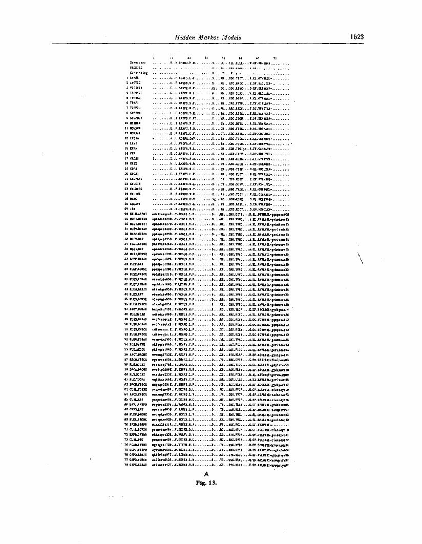
Hidden Markor .Models 1523
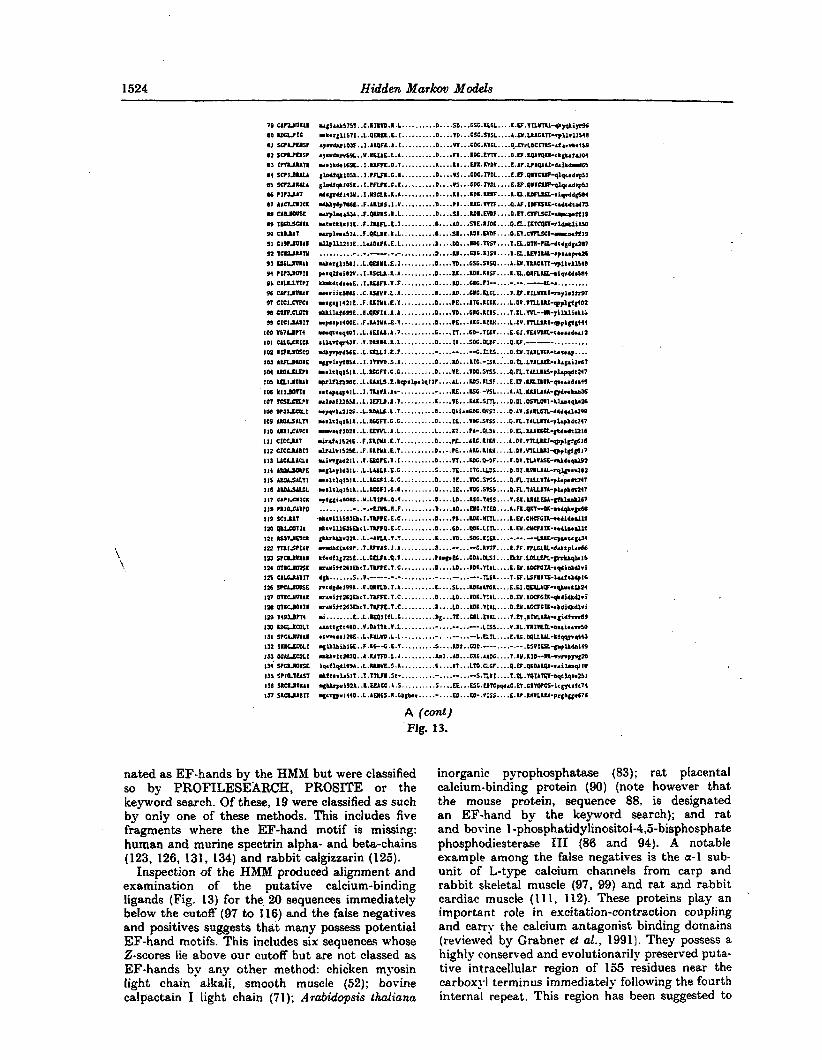
1524 Hidden Markov Models
m'i.~5751 .. C.IItW.t.L .......... D....SD...~C.UCL....I.P.IlLYI11~lgti~ Uk.rgllS?I .. L.PPII.E.1 .......... D....TD...CSC.SISL....A.DI.LCl~-.pll~ll~~ ~,n(.rlR1F..l.ItpFL.l.l..........D-...~...CDC.KlCL....O~.~rlMI1K-~t~..b.iS9 ay.rdarv5'1L..Y.tElAE.L.A .......... D .... FI... KDc.EtlV .... D . ~ . t 4 1 V p P - c b @ d ~ l O 4
m.ikCI69E .. l . W E . D . l . . . . . ..... K .... 1t...LW..KVOI .... E.1F.VMAAI-lrikdb.dM
g M q k I o 5 K .. I . ? M . C . l . . . . . . . . . . D....*5...c=.mL .... E.Q.OllM-#qddlp5J g ~ i * I o I L .. 1 . r N I . c . 1 .......... D . . . . I ~ . . . G ~ . ~ ~ L . . . . I . ~ . ~ ~ ~ ~ ~ ~ , ~ ~ ~ I
IU+y(p7 ~ ~ . . F.11115.l .V... . . . . . . . D....?t ... U C . W m . . . . P . ~ . l D ~ S ~ - ~ ~ * ~ ~ ~ 7 ~ d'p~r4JU .. I . ~ a l . I . 1 . . . . . . . . . . O . . . . I t . . . t D t . l l ~ . . . . I . ~ . M ~ - ~ ~ ~ d ~
wrph.&A..F.WU.I.L .......... D.. ..SI...Mt.EIDF .... O . ~ . o N c I - u n t i l S Yt.IkbIIL..F.IUFL.E.l .......... 0 .... AD...SIC.IIDl.... O.U..IKT~-rld.UiISO urpI..a5JA..F.PILIt.t.L .......... 0 .... SI... MI.EIDF .... P.R.ClTLSCl-u~119 mllplAlllIE..WOIFI.E.L .......... D .... OD ... IPC.mI .... l . a . ~ - ? R - d r ~ ~ A y J n ................................ D....RI..,CDC.KlS~....D.R.~1~-~~~~~~25 U&.qllYI..L.OUII.I.I .......... O....TDD,..C%.SM .... I.P.lUCAR-.plIWIU4O pmqlimi8lU..I.tXU.K.l .......... 0 .... U...IDI.KtSF .... K.R.OlFUP-migrdd&4 Ibld1da.d ..I.?MFL.I.f .._....... D .... M...CtC.fl- .... -.-.---U-a ......... r. . i ic ~ . . C . L Z I V I . L . 1 . . . . . . . . . . D . . . . W . . . C I C . U C L . . . . ~ . ~ . l ~ ~ l - ~ , ~ , j ~ 7 rag~~IlllE..F.UIYA.E.I .......... 0 .... ?E...ATC.LlXY .... L.OP.~1U-spplgtg iDt mUiW699E..ll.aKflA.A.A .......... D .... 'to... ClG.tlIS .... T . D L . m - - I I - y i l U i . k I i -p*.p1400E .. F.KANA.I.1.. ..._.... D .... PE...AIC.LlKY .... L.OV.~lqppl@gi44 u . + . . q 4 O l . . L . L U A l . A . r .......... C .... ll...CC.lILV .... E.CI.VCl9UL-t....&d12
IllmrdYE. .L. pLL1.L.F. . . . . . . . . .-. . . .--. . .-4. ILLS. . . .D. W . l A I L I C K - C 4 % . a p . . . . '
~ U . r t ~ l l .. 1.DUII.L.L. ......... D....lI...SDC.PLOF....O.W.-----.......... r ~ . l . ~ t n ~ .. I . I ~ . S . A .......... D . . . . L D . . . K l C . - l s K . . . . a . a . ~ ~ ~ - ~ ~ g ~ i ~ ~ 7 rlltl~l511 .. L.LCGFl.C.C... .... ... D....VE..-IDe.SlSS .... P.Fl,.TIutAS-pLp9dC247 ~rU~b%E..L.UALS.L.Lqpllplqll~ .... U . . . M % t U F .... E.P.ULIUL-qm.aldl.49
~ l a ~ l U 5 I K .. L . I ~ . l . l . . . . . . . . . . I....VE...Ml.SlT .... P.OL.PsnolI-~h~qblS m~ryup41L..I.NVA.I~- .......... - .... IE...Lzc.- YSL .... 1.1L.UIL1AA-gydlrk~JS u ~ . W I ~ S .. L.LDA~.L.1..........D....OLir~C~.OIS~....O.l~.Sl~~-d~d~~~ 1llclql5lL .. L.LCCn.C.C .......... D. ... IE...lffi.SVSS .... O . F L . l I ~ l - p ~ ~ k d ~ 4 7 rrr.rtIOlY .. L.EL+n.A.L..........L....K1...~I~.~LDA....D.P.UItltL-~d.dcU116 .ir&i&ISl4E..F.KINA.E.Y .......... D .... R... AIC.tIKR .... L.OV.rILLUI-qppl~@I6 ~~~~~~I~BE..F.I~IYI.E.I..........D..-.) mingld21L..V.FtCFE.V.t .......... D....vI...IDc.C-DF .... I.OV.rUlrsL-mkd.glo2
Ugll).ld31L .. L.LAIL1.E.C .......... B . . ~ . ~ . . . I l C . U ~ S . . . . O . D l . ~ W U ~ - ~ ~ l ~ ~ ~ J O l r . l c l q l 5 I K .. L.UCFI.C.C...: ...... D .... lE...IDC.5155 .... O.FL.lIUIlA-pl~p6~241 ~~Itlql5II..L.LCCCI.C.C .......... D .... IE...lDC.SlSS .... O.FL.TILUlI-pkpk6t241 . r fp l . IO.S. .Y .L IVL.P.T .......... D .... LD ... t S C . b J J .... V . f l . U A L F 5 A - ~ k l s n k l 6 7 ......,.._ -..-.-trYI.I.F .......... 0 .... ID...UC.TlEC .... K.FI.OKY-M-m*dqhvpGd ..I~.I~I~O~BII.TLT~L.L.C .......... D .... r ~ . . m . u n ~ .... L.EY.C~CFCR-W~~A..II* ~ 1 . ~ ~ 5 ~ 1 1 - 1 V r n . E . C .......... 0.. .. GO. .. 0 0 K . L l n .... I.W.CEffA~-..di"~lt g ~ U l . 2 ~ 1 .. L . - ~ . U . ~ . ~ . . . . . . . . . . K . . . . ~ . . . S ~ . K I U . . . . - . - - . - - - ~ - ~ ~ ~ ~ ~ ~ L ~ -~.~~~..T.~~P.I.A..........D....-...~.R~....L.F;.~~~~~~~~~~ ki.dfl(22SL .. L.CDfA.0.l .......... IlrEC...CDA.WI .... ~lr.LD~-g7rkkql.l5 ~~~iii2IIO~T.TVFE.t.C .......... D .... LO...tOK.VIIL .... F.W.ACQCI1-meImdl.i dgh ..._... 5..1.-----.-.- .......... - .... --...---. ?.SI .... l.O.LSIttIE-L~irk$16 rrrd~d.d.1)91 .. I . O I M . 1 . L .......... E . . . . S L . . . L D ~ I ~ C K . . . . C . E I . ~ ~ ~ - ~ q k ~ k ~ 2 ~ arriiilBLbcT.lm.1.C .......... D ..._ LD ... IDI.T:lL .... 0.Fd.rccrCtK-qkdidkdlvi Plriii265Lb'T . ~ . l . C .......... 0.. . . L D . i mi ........ E..L.tEOlIiL.C .......... Dg ... lE...COL.CTU .... Y.~.llbUM-.gidtm69 Y . C C @ c l l D .. I . D A l l ~ . V . L ..........-....-...--. L ~ S . . , . V . l L . ~ t I l E U ~ ~ l i ~ ~ ~ 5 0 .I~~~~~E..L.U~YD.L.L..........-. ..--...-- L . O T L .... L . K c . D O U U L - k i ~ ~ 4 3
~ r l r fUa.. l.M~.L.I .......... ~ l . . l D . . . C ~ . l I ~ . . . . l . I ~ , ~ l D - ~ - ~ p ~ ~ ~ y ~ l l l 5 C .. F.KC--C.t.l ..........s.... M~..COD.----....-.--.G5Il~-~~~i49
I ~ i l q d l ~ ) * . . L..UYE.~.I..........C....tl...L~.CLCF....O.~.O1OA~-~~il~~qlIa .wt..I.sIT..T.ms.5t- ...__._... - .... --...- s.nt1 __.. ~.a.rarrmr-.~r~,.ul .gLLrpr5921..t.F.Ucc.1.s .......... s .... ~ . . . a c . o l c ~ ' P . E l . c t ~ ~ c ~ - l ' ~ , . i ' 7 ~ yr*prl((O .. L.l~CS.R.Cbg~. .....-....~...~-. ~ : S ~ . . . . ~ . ~ . ~ ~ ~ - ~ = ~ b ~ ~ 7 6
A (cod! Fig. 13.
nated as EF-hands by the HMM but were classified so by PROFILESEARCH, PROSITE or the keyword search. Of these, 19 were classified as such by only one of these methods. This includes five fragments where the EF-hand motif is missing: human and murine spectrin alpha- and beta-chains (123, 126, 131, 134) and rabbit calgizzarin (125).
Inspection of the HMM produced alignment and examination of the putative calcium-binding ligands (Fig. 13) for the, 20 sequences immediately below the cutoff (97 to 1.16) and the false negatives and positives suggests that many possess potential EF-hand motifs. This includes six sequences whose 2-scores lie above our cutoff but are not classed as EF-hands by any other method: chicken myosin light chain alkali, smooth muscle (52); bovine calpactain I light chain (71); Arabidopsis thaliana
inorganic pyrophosphatase (83); rat placental calcium-binding protein (90) (note however that the mouse protein, sequence 88, is designated an EF-hand by the keyword search); and rat and bovine 1 -phosphatidylinositol-iij-bisphosphate phosphodiesterase I11 (86 and 94). A notable example among the false negatives is the a-l sub- unit of L-type calcium channels from carp and rabbit skeletal muscle (97, 99) and rat and rabbit cardiac muscle (1 11, 112). These proteins play an '
important role in e.ucitstion-contrsction coupling and carry the calcium antagonist binding domains (reviewed by Grabner et at., 1991). They possess a highly conserved and evolutionarily preserved puta- tive intracellular region of I55 residues near the carboxyl terminus imrnediat.ety following the fourth internal repeat. This region has been suggested to
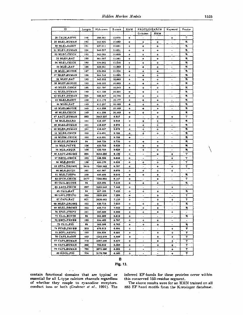
Hidden Markor Models 1525
B Fig. 13.
contain functional domains that are typical or inferred EF-hands for these proteins owur within essential for all L-type calcium channels regardless this cbonserred 155-residue segment. of whether the?; couple to ryanodine receptors. The above results were for an H3131 trained on all conduct ions or hoth (Grahner cf nl. . 1991). The 885 EF.hnnd motifs ft-nln the Krt.tsjI1pr dntahar .
. ..
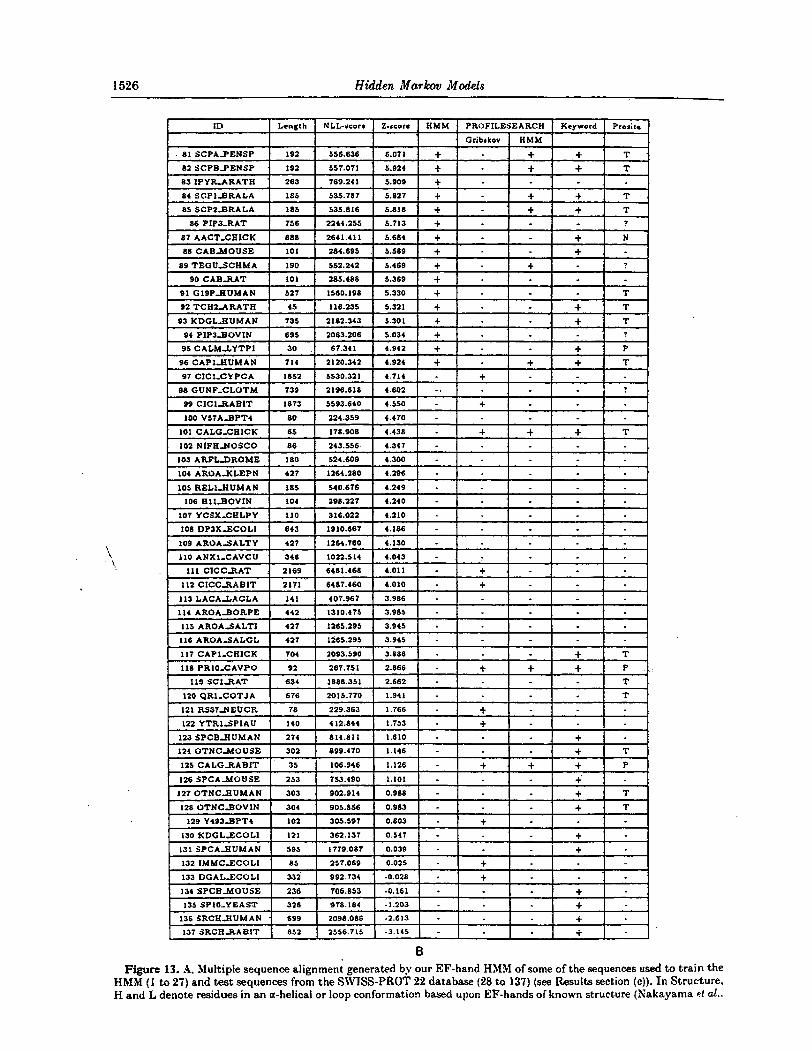
1526 Hidden Markov Bodels
\ i '.
B Figure 13. A, Multiple sequence alignment generated by our EF-hand HMM of some of the sequences used to train the
HMM (1 to 27) and test sequences from the SWISS-PROT 22 database (28 to 137) (see Results section (c)). In Structure. H and L denote residues in an a-helical or loop conformation based upon EF-hands of known struct.ure (Xakayama rf d..

Hidden Markov Models 1527
There is considerable overlap between this training set and the EF-hand motifs found in SWISS-PROT 22, so in order to provide some clearer cross valida- tion of our results we also did another series of experiments. In these experiments, models were estimated using training sets consisting of different numbers of randomly chosen EF-hand sequences from the database of 885 EF-hand sequences. For training sets consisting of 5, 10, and 20 random EF-hand sequences, 15 models were estimated, each using a different randomly chosen training set. For training sets consisting of 40, 80, 100, 200, and 400 random EF-hand sequences, five models were esti- mated. In all, 70 models were estimated. A model's performance after training was gauged on how well i t performed on a test set which consisted of motifs from the database of 885 sequences that were not used in the training set. Thus for each model, two XLL-scores were computed (see Methods section ( f ) ) , one for the training set and one for the test set.
- These XLL-scores serve as a quantitative measure of hoG well the model is representing the sequence data. Figure 14 shows that for small training set sizes, the model overfits the training data. This is shown by low training NLL-scores but very high testing XLL-scores. This effect largely disappears when the training set size reaches about 100 sequences.
A model's performance was also gauged on how well i t searches a database for sequences containing the EF-hand motif. For each training set size, one model was randomly chosen to search SWISS-PROT 22. A histogram of the resultant Z-scores was plotted and a cutoff was chosen by eye. The number of false positives was computed, as
Tmining ssl Sam
Figure 14. Average XLL scores for test and train sets for models with training sets of size 5, 10: 20, 40, 8 0 , 100, 200 and 400. Error bars represent one standard deviation.
described earlier in this section, by taking a list of certain EF-hands (i.e. determined to contain the EF-hand motif by the 3 independent sources) 8.4 counting the number of sequences above the 2-score cutoff in the HMM database search that were not in the certain EF-hand list. Figure 15 shows that models built from smali training sets have large numbers of false positives. Again, this effect dis-
1992). PROSITE denotes the positions used to generate the pattern EF-HASD. Ca-binding identifies t h e 6 residues involved in octahedrally coordinating the calcium ion (denoted by X, 5'. 2. x, z and y). The oxygen atom at. position y comes from the main-chain and so can be supplied by any amino acid. Sequences 1 t o 27 are representatives of the various EF-hand subgroups in the June 1992 database of EF-hand sequences maintained by Kretsinger and co-workers (K'skaysma et al., 1992). These sequences are: CAMHS, Homo sapiens calmodulin; a A C . G , Callus gallus a-actinin; VISIKIX, G. gullua visinin; TPP24CF. Canis jamiliaria p24 thyroid protein; TPHUCS, H. sapiens skeletal troponin-C; TPAPl? l s t a c w ponlasliew troponin-C-1: TCBP25, Tetmhymena themophila TCBP-25; SPEMA, h70ngyloceutmha p p r d w speck; SCBPBLI. BranchiosW lanceolatum SARCl; QUIDLX? Loligo peulei squidulin; MOHSCR, H. sapiens myosin (RLC-ventricle); MOHSA1, H. sapiens myosin (ELC-LI-skeletal); LPSlA, Lylechirus p i d w a-Lpsl;. LAVl, Physamrn polycephulum LAW-2; EFH5, Tlypanosoma b m e i putative calcium binding protein; CVP, 3. Zance&um calcium vector protein; CRGHS. H. sapiens celmodulin-ielated gene; CMSE, Saccharopolysy eythraea bacterial-CAM; CDPK, Glycine tmxz calcium. dependent protein kinase: CDC31, Saccharomyces cererisiae ce11 division control protein 31; CALPLHS. H. sapiens calpain (light): CALCIB, Bos taurw calcineurin-B; CALBXGG, 0. gdZus caibindin; CALICE, Ctwmhbdab elegana cal 1 gene; BCHS, H. sapiens fi 5-100 protein; AEQAV1. rleqzwrea victuria aequorin-1; and 1F8, Try?lanosoma cruzi flagellar calcium binding protein. 28 to 96 are the SWISS-PR.OT 22 siquences designated as EF-hands by our HMM (2-score >475) but not by all 3 other methods, PROSITE, PROFILESEARCH and the keyword search. Biote that sequences identified as EF-hands by all 4 methods are not. shown. 97 to 116 are t.he top 20 sequences below our cutoff of 475; 117 to 137 are sequences that were not. classified as EF-hands by the HMM but were so by one or more (but not all) of the 3 other methods. B, Details on sequences 18 to 137 shown in the alignment (arranged in order of decreasing 2-score). XLL-score and 2-score are measures of how well the EF-hand HMM fits these database test sequence tha t were not present in the training set (see Results section (c) for more details). Tn HMM. PROFILESEARCH. Keyword and PROSITE + and - denote sequences that are and are not. respctively. classified BS containing an EF-hand motif by the 4 specified methods. For PROFILESEARCH. Cribskov and HMM indicate results based upon profiles generated from four EF-hand sequences and our HMMM alignments. T. X. P and ? in PROSITE have the same meaning LIS in Fig. 11. ?& indicates sequences which possess an EF-hand motif bur do not bind calcium.

NUlTJ2Wlr&inQni*rg5equarar
Figure 15. EF-hand database search false positires for models trained with 5. 10. 20. 40. 80. 100. 200 . 400 and 885 sequences.
~~ ~ ~ ~~ ~ ~ ~ ~~ ~~ ~~~ ~~
appears substantiall? when the training set size reaches a.bout 100 sequences.
4. Discussion 'i, X new method to model protein families using hidden Markor models has been introduced. The method is capable of tapping into the tremendous amount of sta.tistical information contained in many unaligned sequences from the Same family. For the cases of globins: kinases and EF-hands. the results have shown that by using this method. it is possible to obtain multiple alignments that mirror structural aIignments, having anly the unaligned primary sequences as input. The results h a w also shown that the model can be used successfully in database searches for putative analogs of srquenc.es in a given protein family or domain. Finally. we believe that the model itself is a oaluable tool for representing the family or domain.
The HYJI method we have proposed requires that many sequences be available from the family o r domain one wants to model. Since the nurnl~er of sequences in the protein databases i s growing rapidlj-, this may be less of a problem i n the future. but it will always he a serious issue. Currently. only a relatively small number of sequences are avai1nt)le for most protein families and domains. For the globin family, we found that 400 sequenres is certainly sufficient. Preliminary., results indicate that 200 is enough, and even as few as 70 may sufice if they are chosen~'carefully from our data- base of 6-28 (70 chosen at random w i l l l~ nearly all a- and &chains). Our experiments using snlaller numbers of EF-hand sequences for. training. as described in Results section (0 ) . show a similar
might even be lowered further. However, there will be a limit on how small the number of available sequences can be if one hopes to obtain a reasonable model starting from a tabula rasa.
We believe that the answer to the problem of small training sets is to add more prior knowledge into the training process. One way to do this is by starting with a better initial model. We have per- formed several experiments in which we have started with a model obtained from a small st of aligned sequences, and then trained the model further using a larger set of unaligned sequences. These will be reported in a future paper. We find that this technique can often give better results. This also suggests that one application of HMMs may be in maintaining multiple alignments as the number of sequences in the alignment grows. Each time new sequences are added to a dataset of homo- logous sequences. we can begin with the HMM based on the alignment of the previous set of sequences, train it with the larger dataset that includes the new sequences. and then create a new multiple align- ment for the larger dataset from this HMM. Xot only \vi11 the new sequences be included in the new alignment. but the alignment of the old sequences may be improved by utilizing the statistical information present in the larger dataset.t
.\nother way to add more prior knowledge into the training process is to use a more sophisticated Bayesian prior. We are currently exploring the use of a prior on the probability distribution over the amino acids in a match state of the model consistine of a misture of Dirichlet priors(8rown et ai., 1993). Vsing such a prior is like "soft-tying" the distribu- tions in the states of the HJIM. By soft-tying we mean a combination of the idea of tying states (see e.g. Rahiner. 1989). in which the number of free parameters is reduced by having groups of states all sharing the same distribution on the output alphabet (the 20 amino arids in this case), and the idea of soft weight sharing from Sowlrin t Flinton (1992). i n which the regularizer (in this, case the prior for the tlistrilmtion of amino acids) is also adaptirdy motlifird during learning. LVe have shown that this method can be used to estimate good KF-hand models using substantially fewer training sequenvez. Other types of more sophisti- cated priors can be obtained by switching from the alphal)st of the prirnar_v sequences to a different representation Imed more on the structural or chemical properties of the amino acids in the sequence. W e plan to explore these as well-
It is interesting to note that \{-e have obtained quite gootl results i n multiple alignment and data. base searching without using any special weighting schemes to rnakr up for the statistical bias in OUI training sets (see e.g. Sibbald Br Argos, 1990), 01
employing Ihyhoffs matrix or any of its analog! (see e .g . IVatrrman. 1989) to take explicit rnutatior
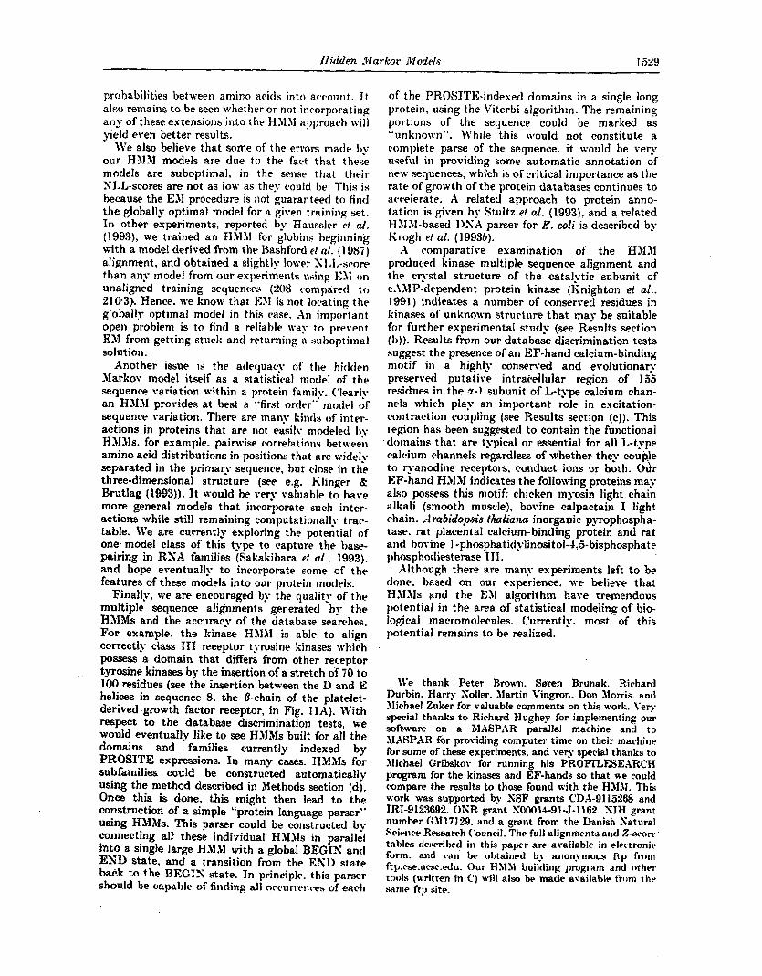
probabilities between amino acids into account. 1 t also remains to be seen whether or not incorporating any of these extensions into the HMJl approach w i l l yield e\-en better results.
We also believe that some of the errors ma.tle I)? our HJIM models are due to the fact that these models are suboptimal, in the sense that thrir XLL-scores are not as low as they c~ould be. This is because the E31 procedure is not guaranteed to find the globally optimal model for a given training set. In other experiments, reported by Hanssler rt al. (1993), we trained an HMJI for.globins beginnink with a nlodel derived from tlw Bashford et al. (1 !Mi) aJignment, and obtained a slightly lower SI.I.-scow than an?- model from our esperilnrnts wing E:JI on unaligned training sequences (208 compiretl t o 210.3). Hence. w e know that 1511 is not locating the globally optimal model in this case. An important open problem is to find a reliaMe way to prevent Ell from getting sturk and returning a suboptimal solution.
Another issue is the adequacy of the hidden Markov model itself as a statistical model of the sequence variation within a protein family. (‘learly an H3IN provides at best n **first ortlrr” nmtlel of sequence variation. There are many kinds of inter- actions in proteins that are not easily nodel led I)? HJIJls. for esample. painvise correlations between amino acid distributions in J)OSitionS that are widely separated in the primary sequence. but close in the three-dimensional structure (see e.g. Klinger & Brutlag (1993)). It would he very raluable to hare more general models that incorporate such inter- actions while still remaining computationally trac- table. We are currently exploring the potential of one. model class of this type to capture the base- pairing in RSA fa.milies (Sakakibara ct ai.. 1993). and hope eventually to incorporate some of the features of these models into our protein models.
Finallv, we are encouraged by the quality o f the multiple sequence alignments generated by the HMMs and the accuracy of the database seawhes. For example, the kinase H3lY is able to align correctly class TIT receptor tyrosine kinases which possess a domain that. differs from other receptor tyrosine kinases by the insertion of a stretch Of 70 to 100 residues (see the insertion between the 1) and E helices in sequence 8, the /I-chain of the platelet- derived growth factor receptor, in Fig. I ]A). k17ith respect to the database discrimination tests, we would eventually like to see HX’vIs built for all the domains and families currently indexed by PROSITE expressions. In many cases. HMMs for subfamilies could be constructed automatically using the method described in Methods section (d). Once this is done, this might then lead to the construction of a simple “protein language parser” using HJi3I.s. This parser could be constructed by connecting all these individual H M h in parallel into a single large HMM with a global BEGIX and Ex’1) state, and a transition from the ESD state back to the BECTS state. In principle. this parser should be cqal)te of finding all n(vurrt*tl(*es of eacsh
of the PR.08ITE-indexed domains in a single long protein, using the Vit.erbi algorithm. The remaining portions of the sequence could Ire marked as “unknown“. While this would not constitute a eomplete parse of the sequence. it would be very useful in providing some automatic annotation of new sequences, which is of critical importance as the ra.te of growth of the protein databases continues to accelerate. A related approach to protein anno- tatiou is given by Stultz et al. (1993). and a related FlJIJI-based 1)SA parser for E. coli is described by Krogh et ai. ( I 9936).
A comparative examination of the HMM produced kinase multiple sequence alignment and the cqstal structure or the catalytic subunit of c.4MP-dependent protein kinase (Knighton el al.. 1991) indicates a number of conserred residues in kinases of unknown structure that may be suitable for further experimental study (see R.esults section ( I ) ) ) . Results from our database discrimination tests suggest the presence of an EF-hand calcium-binding motif i n a highly conserved and evolutionary preserved putative intracellular region of 155 residues in the 2-1 subunit of L-type calcium chan- nels which play an important role in excitation- cmtraction c*oupling (see Results section (c)). This region has been suggested to cont-ain the functional domains that are typical or essential for all L-t.ype calcium channels regardless of whether they coup!e to ryanodine receptors, conduct ions or both. O h EF-hand HMJI indicates the following proteins may also possess this motif: chicken myosin light chain alkali (smooth muscle), bovine calpactain I light chain. -4 rabidopeis trllaliunn inorganic pyrophospha- tase. rat placental caleiam-binding protein ancl rat and bovine 1 -phosphatidylinositol-4,5-bisphosphate phosphocliesterase 111.
Although there are many experiments left to be done. based on our esperience. we believe that HJIJIs Hnd the E31 algorithm have tremendous potential in the area of statistical modeling of Wo- logicd macromolecules. Currently. most of this potential remains to be rea.lized.
We thank Peter Brown. Smen Brunak. Richard Durbin. Harry Soller. Martin Vingron. Don Momis. and Michael Zuker for valuable comments on this work. \-my special thanks to R,irhard Hughey for implementing our soft.ware on a MASPAR. parallel machine and to YASPAR for providing computer time on their machine for some of these experiments. and very special thanks to Michael Gribskor for running his PROFILFSEAR.CH program for the kinases and EF-hands so that we muld rompare the results to those found with the HIIN. This work was supported by XSF grants CDA-9I16fW and TRT-9123692. OXSR grant SooO1+915-1162. XIH grant number 03117129. and a grant fmm the Danish Satural Srin1c.r Research (‘ouncil. The full a1ignment.s and Z-xc~ore tahles dewribed i n this paper are arailabte in elertronic form. ancl (*all be obtained by anonymous ftp fronl ftp.rse.ucsc.edu. Our HMLI builclinp program and other tools (written i n C‘) will also be ma& availahlr frcm thr salne f t ~ ~ site.

I530 Hidden Markov Models
References
Xbe. S. 8- Warmuth. SI. (1990). On the compubational complexity of approximating distributions by probabilistic automata. In Proceedings of the 3rd Workshop OR C o m p u l a l i d Learning Theoy . pp. 5'2-66. Morgan Kaufmann, Rochester. ST.
Allison. L.. Wailace. C. S. & Yee, C. X. (1992). Finite-state models in the alignment of macromolecules. J . Md. Evd. 35, 77-89.
Asai. K.. Hayamizu. S. & Onizuka, K. (1993). HMM with protein structure grammar. In Proceedings of the Hawaii Intermtiom1 Conference on System Scielrces. pp. 783-i91. TEEE Computer Society Press. Los Alamitos. C.1.
Bairoch. X. (1992). Prosite: a dictionary of sites and patterns in proteins. Nucl. Acids Res. 20.1013-2018.
Baldi. P. 8: Chauvin. 1'. (1993). A smooth learning algorithm for hidden Markov models. ,Veural Computation, in the press.
Baldi, P.. Chaurin, Y., Hunkapiller, T. 8 " h e . 11. X. (i993). Hidden Markov models in molecular biology: new algorithms and applications. In Adzurnces in SeuraE Information Processing Systems 5 (Hanson. Coran 8- Giles. eds), pp. 7-47-72. Morgan Kauffmann Publishers. San Mateo? CA.
Barton. G. J. (1990). Protein multiple sequence alignment and flexible pattern matching. Method8 Enzymol. 183, M3428.
Barton, C. J. 8: Sternberg. M. J. (1990). Flexible protein sequence patterns: a sensitive method to detect. weak structural similarities. J . Xo l . Biol. 212 (2): 389-402.
Bashford. D.. Chothia, C. h Lesk, X. 11. (1987). \ Determinants of a protein fold: unique features of the i. globin amino sequence. J . Mol. Bid. 1%: 199-216.
Berger, J. (1985). Stalistical Decision Theory and Bayesian Analysis. Springer-Verlag, Xew Tork.
Bowie. J. C.. Liithy, R. 8 Eisenberg, D. (1991). A method to identify protein sequences that fold into a known three-dimensional structure. Science. 253: 164-170.
Brown. X. P.. Hughey. R., Krogh. A.. Mian. I. S.. Sjolander. K. & Haussler, D. (1993). C'sing Dirichlet mixture priors to derive hidden Markov models for protein families. In Proc. Firsf Int. PonJ on tnklligenf System for ;Molecular Biology (Hunter. L.. Searls. D.. Sharik. J.. eds), pp. 17-55. AhAI Press. Wash. D.C'.
Cardon, L. R. & Storrno. C. D. (1992). Expectation maximization algorithm for identifying protein- binding sites with rariable lengths from unaligned DX.4 fragments. J . Y d . Biol. 223. 159-110.
, Churchill, G. A. (l-989). Stochastic models for heterogeneous DSA sequences. Bull Xath Biol. 51. 79-94.
Dempster. A. P.. Lai rd , X. M. 8 Rubin. D. 8. (1977). Maximum likelihood from incomplete data r ia the EM algorithm. J . Roy. Statisf. Sa. 5. 39. 1-38.
Dickerson. R.. E. & Geis. I. (1983). Hemoglobin: Stttuetrre. Function. EtaIuiion a d Pathology. Benjamin/ Cummings Pub. Co, Menlo Park, CA.
Duda. R. 0. & Hart. P. -E. (1973). Ptzflem Cla.ssijicution and Scene Anulysis. Wiley. Xew York.
Everitt, B. S. 8; Hand. D: J. (1981). Finite Mirture Dislribdions. Chapman and Hall, London.
Feng, D. F. 8: Doolittle, R. F. (1987). Prc -si 'c sequence alignment as a prerequisite to correct phytogenetic trees. J . Mol. Pvol. 25, 351-360.
Garbem. D. L. (1992). Guanylyl cyclase receptors and
their endocrine. paracrine and autocrine ligands. cell, 71. 1-4.
Chnan. S.. Bienenstock. E. & Doursat, R. (1992). Neural networks and the biastvariance dilemma. N e u d Compdation. 4. 1-58.
Grabner. SI.. Friedrich, K., Knaus. H.-G., Striessnig, J., Scheffauer. F.. Staudinger, R.. Koch. W. J., Schwartz. A. &. Glossmann, H. (1991). Cahium channels from Cyprinus carpi0 skeletal muscle. Proc. .Val. dead. Sci.. U.S.A. 88. 727-731.
Gribskov. 31.. Liithy, R. & Eisenberg. D. (1990). Profile analysis. Methala EnzymZ. 183, 146159.
Hanks. S. K. & Quinn, A. M. (1991). Protein kinase catalytic domain sequence database: identification of conserved features of primary structure and classification of family members. Yethod8 Enzymol.
Hanks. S. K., Quinn. A. M. 8 Hunter. T. (1988). The protein kinase family: conserved features and deduced phylogeny of the catalytic domain. Scienee.
Haussler. D. 8: Krogh. A. (1992). Protein alignment and clustering. Presented at the conference SeuraI Setworks for Computing.
Haussler. D.. Krogh. A., Mian. I. S. & Sjolander, K. (1992). Protein modeling using hidden Markov models: analysis of globins. Technical Report N"CC-CRL-92-23 Universit? of California at Santa Cruz. Computer Science Dept.. Santa Cruz, CA 95064.
Haussler. D.. Kmgh. A.. Mian, I. S. & Sjiilander, K. (1993). Protein modeling using hidden Markov models: analysis of globins. In Proecedings of the Hawaii Inlernutional Conference on System Sciences, IEEE Computer Society Press. Los Alamitos, CA.
Hunter. T. (1991). Protein kinase classification. Methode E R Z I J ~ M O ~ . 200. 3-37.
durka. J . 8: Slilosavljeric, A. (1991). Reconstruction and 'analysis of human Alu genes. J . .\id. Ecol. 32. 105-121.
Klinger. T. B: Brutlag. D. (1993). Detection of correlations in tRSA sequences with structural implications. In First InternalimaI Conference on Inteiligenl Systems for .Ifdecular Biology (Hunter. L.. Searls, D. B: Sharlik. d.. eds). A A A I Press. Menlo Park.
Knighton. D. R.. Zheng. J.. Eyck. L. F. T.. Ashford. V. .I.. Strong. S.-H.. Taylor. S. 8. d: Sowadski. J. M. (1991). Crystal st.ruc?ture of the catalytic subunit of c:\clit adenosine monophosphate-dependent protein kinase. Science. 253. 407414.
Krogh. A . . Brown. SI.. Mian. I . S.. Sjolander. K. 8. Haussler. D. (199b). Hidden Markov models in conlputational biolokv: applications to protein modeling. Technical Report CCSC-CRL-93-32 I'nirersity of California at Santa Cruz. Computer Science Dept., Santa Cruz. CA 95064.
Krogh. -4.. Mian, I. S. & Haussler, D. (1993b). A hidden Markov model that finds genes in E . coli DXA. Technical Report UCSC-CRL-93-33 Cnivemity of California at Santa Cruz. Computer Science Dept.. Santa Cruz. CA 95064.
lander. E. S. & Green. P. (1987). Construction of multilocus genetic linkage maps in humans. Proc. S a t . h a d . Sci., U.S.A. 8 4 , 23634367.
Lawrencp. C . E. 8; Reilly. A . A. (1990). An expctation maximization (EM] algorithm for the identification anti characterization of cammon sites in unaligned biopcl. mer sequences. Proteins. 7. 41-5 I .
Lindherg. R. X.. Quinn. A. 11. 8: Hunter. T. !1992)
200.38-62.
241. q2-5'2.
Hidden Markov Jlodels 1331
Jhal-specificity protein kinases: will any hydroxyl do? Trends Biochem. Sci. 17. 114-1 19.
Liithy. R.. McLachlan. A. D. 8: Eisenberg. D. (1991). Secondary structure-based profiles: use of structure- conserving scoring table in searching protein sequence databases ’ for structural similarities. Proteins: Slnrcl. Funcl. Gene!. 10, 229-239.
Moncrief. S. D., Kretsinger. R. H. 8; Goodman. M. (1990). Evolution of EF-hand calcium-modulated proteins. T.. Relationships based on amino acid sequences.
Sakayama. S., Moncrief. X. D. L? Kretsinger, R. H. (1992). Evolution of EF-hand calcium-modulated proteins. 11. Domains of several subfamilies have diverse evolutionary histories. J . 2 0 ! . Evot. 34, 4 1 6 4 4 8
S o d a n . S. (1990). Maximum likelihood competitive learning. I n Advances in Neural Infwmalion Prmessing Sysfems (Touretsky. D.. ed). vol. 2. pp. 574-582. Morgan Kaufmann. San Jlat,eo. CA.
Sowlan. S. J . & Hinton, G . E. (1992). Soft weight- sharing. In Advances in Seural Information Processing System 4 (Moody. Hanson 8: Lippmann. eds). 3iorgan KaufTmann Publishers. San Mateo. CA.
Persechini. A.. Moncrief, X. D. & Kretsinger. R. H. (1989). The EF-hand family of calcium-modulated proteins. Trends Weurosei. 12 (1 1 ), 462-467.
Rahiner, L. R. (1989). A tutorial on hidden Markov models and selected applicat.ions in speech recognition. Prm IEEE. 77 (2). 25-286.
Sakakibara. Y.. Brown. Y., Underwood, R.. Man. I. S. & Haussler. D. (1993). Stochastic context-free
J . Mol. Evo~. 30,5’22-562.
grammars for modeling RIGA. Technical Report UCSC-CRL-93-16 University of California at Santa Cruz. Computer Science Dept., Santa Cruz, CA 95064.
Sibbald, P. & Argos, P. (1,990). Weighting aligned protein or nucleic acid sequences to correct for unequal representation. J . Mol. Biol. 216, 813-818.
Stultz, C. M., White. J. V. & Smith. T. F. (1993). Structural analysis based on state-space modeling. Protein Sei. 2, 305-315.
Subbiah. S. & Harrison, S. C. (1989). A method for
209.534-548. multiple sequence alignment with gaps. J . Mol. Biol.
Tanaka, H.? Ishikawa, M., Asai, K. & Konagaya, A. (1993). Hidden Markov models and iterative aligners. In First I n l e d i d , Conference on Indelligenl Systems for Ydecular Biology, . U A I Press, Menlo Park.
Taylor. IV. R. (1986). The classification of amino acid Conservation. J . Theoret. Biol. 119. 205-218.
Vingron. 11. & Argos. P. (1991 ). Motif recognition and alignment. for many sequences by comparison of dot- matrices. J . Mol. Bwl. 218, 33-43.
Waterman, 11. S. (1989). Sequence alignments. In Nafhematieal Yeflrods for DXA Sequences (Waterman. 31. S., ed.). CRC Press, Boca Raton, FL.
Waterman. Y. S. & Perlsitz, 1. D. (1986). Line geometries for sequence ‘comparisons. Bull. &fa& Biol. 46. 567-577.
White. J. Y., Stultz, C. M. & Smith, T. F. (1991). Protein classification by nonlinear optimal filtering of amino- acid sequences. Unpublished manuscript.
’\ Edited by F . Cohen
(Received 4 January 1993; accepted 23 September 1993)