NASA Contractor Report 201727

ICASE Report No. 97-41

3ARY

COMPUTATIONAL ISSUES IN DAMPING

IDENTIFICATION FOR LARGE SCALE

PROBLEMS

Deborah E PilkeyKevin P. Roe

Daniel J. Inman

NASA Contract Nos. NAS1-19480, NAS1-97046

August 1997

Institute for Computer Applications in Science and Engineering

NASA Langley Research Center

Hampton, VA 23681-0001

Operated by Universities Space Research Association

National Aeronautics and

Space Administration

Langley Research Center

Hampton, Virginia 23681-0001

https://ntrs.nasa.gov/search.jsp?R=19970028853 2018-07-28T15:23:37+00:00Z

Computational Issues in Damping Identification

for Large Scale Problems*

Deborah F. Pilkey

Engineering Scicncc _ Mechanics

Virginia Polytechnic Institute

Blacksburg, Virginia 24061-0219

dpilkey©vt, edu

Kevin P. Roe

ICASE

NASA Langley Research Center

Hampton, Virginia 23681-0001

kproe_icase, edu

Daniel J. Inman

Engineering Science & MechanicsVirginia Polytechnic Institute

Blacksburg, Virginia 24061-0219dinman_vt, edu

Abstract

Damage dctection and diagnostic techniques using vibration responses that depend on analytical

models providc more information about a structure's integrity than those that arc not model based.Thc drawback of these approaches is that some form of workable model is required. Typically, models

of practical structures and their corresponding computational cffort arc very large. One method of

detecting damage in a structure is to measure excess energy dissipation, which can bc seen in damping

matrices. Calculating damping matrices is important because there is a correspondence between a

change in the damping matrices and the health of a structure. The objective of this research is

to investigate the numerical problems associated with computing damping matrices using inversemethods.

Two damping identification methods arc tested for efficiency in largc-scale applications. One is an

iterativc routine, and the other a least squares method. Numerical simulations have been performed

on multiple degree-of-freedom models to test the effectiveness of the algorithm and the usefulness of

parallel computation for the problems. High Performance Fortran is used to parallelizc the algorithm.

Tests were performed using the IBM-SP2 at NASA Ames Research Center.

Thc least squares method tested incurs high communication costs, which reduces the benefit of

high performance computing. This method's memory requirement grows at a very rapid rate meaningthat larger problems can quickly exceed available computer memory. The iterativc method's memory

requirement grows at a much slower pace and is able to handle problems with 500+ degrees of freedom

on a single processor. This method benefits from parallelization, and significant speedup can be seen

for problems of 100+ degrccs-of-freedom.

*This research was supported by the National Aeronautics and Space Administration under NASA Contract Nos.NASA-19480 and NAS1-97046, while the authors were in residence at ICASE, NASA Langley Research Center, Hampton,VA 23681-0001.

1 Introduction

The synthesis of damping in structural systems and machines is extremely important if the model is

to be used in predicting transient responses, transmissibility, decay times, or other characteristics in

design and analysis that are dominated by energy dissipation. Methods for determining the mass and

stiffness matrices of a system are more straightforward than those for determining the damping matrix,

as they represent quantities which can bc measured and evaluated by static tests. Damping, on the other

hand, must bc determined by dynamic testing. This makes the process of modcling and experimental

verification difficult. It is assumed here that acceptable models of the mass are available and that it

is desired to use either the cigcnvalue and eigenvector, or transfer function information to construct a

damping matrix. This is known as an invcrsc problem.

One application of the inverse problem is diagnostics. This idea is to test for changes in a structure's

properties by looking at changes in measurable values such as mode shapes or frequencies. Here the

underlying assumption is that changes in the damping values correspond to some sort of change in thestructure's health.

A factor not yet investigated in damping identification is how the problem size affects the ability

to solve the inverse problem. Although most example problems used in publishcd papers are able to

prove that a mcthod is capable of producing the desired results for small problems, it is usually not

mentioned whether a particular method is still viable when the problem size is increased to practical

limits with many degrees of freedom. Most inverse problems in damping identification require some sort

of iteration or optimization procedure. These can become very costly with the increasing problem size

in regards to execution time and computer memory limitations.

The increased execution time and required computer memory creates a need for high performance

computing. Parallel machines can provide a decreased execution time when the workload is distributed

among multiple processors and if the data is also distributed then the per processor memory requirement

may be decreased as well. At least two ways of programming parallel computers are available. Hand-

coded message passing can be done and may achieve excellent performance at the price of a long

conversion process. This approach forces the programmer to explicitly handle the low-level details

of the required communication and to hardwire the choices into the code. This makes the program

difficult to understand and inflexible. The other method is for a compiler to handle the parallelization

of a sequential code. High Performance Fortran (HPF) allows the programmer to parallelizc a sequential

code while only requiring the addition of a few data distribution directives at the top of the code. HPF

has a much lower learning curve and handles most of the low level optimizations without the user's

knowledge. This means good performance can be achieved while abstracting away the details.

In the following paper, Section 2 describes several methods used in damping identification. Sec-

tion 3 is an introduction to the capabilities and uses of High Performance Fortran. Next, two recent

representative damping identification routines are described in detail. A sample problem is presented,

and the parallelization procedure is explained for both methods. Examples are followed by results andconclusions.

2 Background

The problem being investigated assumes a structural system consisting of mass (M), damping (C), and

stiffness (K) matrices such that the response x(t) satisfies

MJ/+ C:_ + Kx = 0, (1)

where x is an n by 1 vector varying with time, representing the displacements of the masses in a lumped

mass system (n is the number of degrees of freedom). The vectors 5_ and _ represent the acceleration

and velocity respectively of the lumped masses.

The idea behind an inverse problem is to find the physical parameters of a system (mass, damping,

and stiffness) from its behavior using measurements such as forced responses and natural frequencies.

Damping identification is an inverse problem in which the damping matrix is the desired result.

Matrix identification can bc done by several methods, many of which are described below. Several

approaches make limiting assumptions such as diagonal or proportional damping matrices, while others

assume the experimental data is incomplete and use only partial eigensystems to solve for damping.

Caravani and Thomson (1974) developed a method for damping identification specific to viscous

damping. In their iterative method, thc goal is to minimize the real and ideal response vectors. This

method is meant to solve relatively simple problems and requires that the "true" response bc known

a priori. Fritzen (1986) optimizes a loss function in his Instrument Variable method. This method

requires a full set of measurement information, but works well when noise is added to the system. It is

not necessary for this method to have a prior model of the system. This instrument variable method is

itcrative, but requires few iterations. It is in the frequency domain, and works best when damping is

large. Several methods are combined in a paper by Roemer and Mook (1992). Noisy measurement data

are used to identify properties of lumped parameter systems by combining two time domain techniques

and an estimation technique. Hasselman (1972) uses perturbation theory to solve for the damping

matrix of the systems with small, proportional damping. Linear viscous damping is assumed.

3 Introduction to High Performance Fortran

High Performance Fortran (HPF) was designed to provide a portable extension to Fortran 90 for writing

data parallel applications. It includes features for mapping data to parallel processors, specifying data

parallel operations, and methods for interfacing HPF programs to other programming paradigms. It is

expected that HPF will bc a standard programming language for computationally intensive applications

on many types of machines, including massively parallel MIMD (Multiple Instruction Multiple Data)

and SIMD (Single Instruction Multiple Data) multiprocessors as well as traditional vector processors.

Features of HPF include compiler directives, parallel constructs, array intrinsics, and escape mecha-

nisms for interfacing with other languages and libraries. Compiler directives are structured comments

that assert facts or suggest implementation strategies about a program to the compiler (Koclbcl, ct al,

1994). HPF directives allow the programmer to specify how to assign array elements to the memory

of processors. Data mapping can bc accomplished by using DISTRIBUTE statements which partition

the data over the processors in a BLOCK, CYCLIC, or general CYCLIC(m) manner. In a BLOCK distribu-

tion, contiguous blocks of the array arc distributed across the processors. In a CYCLIC distribution,

array elements arc distributed among processors in a round-robin fashion. In a CYCLIC (m) distribution,

contiguous data blocks of size m arc distributed cyclically. The ALIGN directive tells the compiler how

different arrays arc aligned with each other to reduce intcrprocessor communication. The combination

of alignment and distribution defines how the arrays arc mapped. Data parallel operations can bc

specified using parallel constructs such as FOIL_LL and INDEPENDENT.

4 Least Squares method

Chcn, Ju, and Tsuci (1996) developed a method in the frequency domain that can solve for the damping

matrix independent of the mass and stiffness matrices, using data obtained from a frequency response

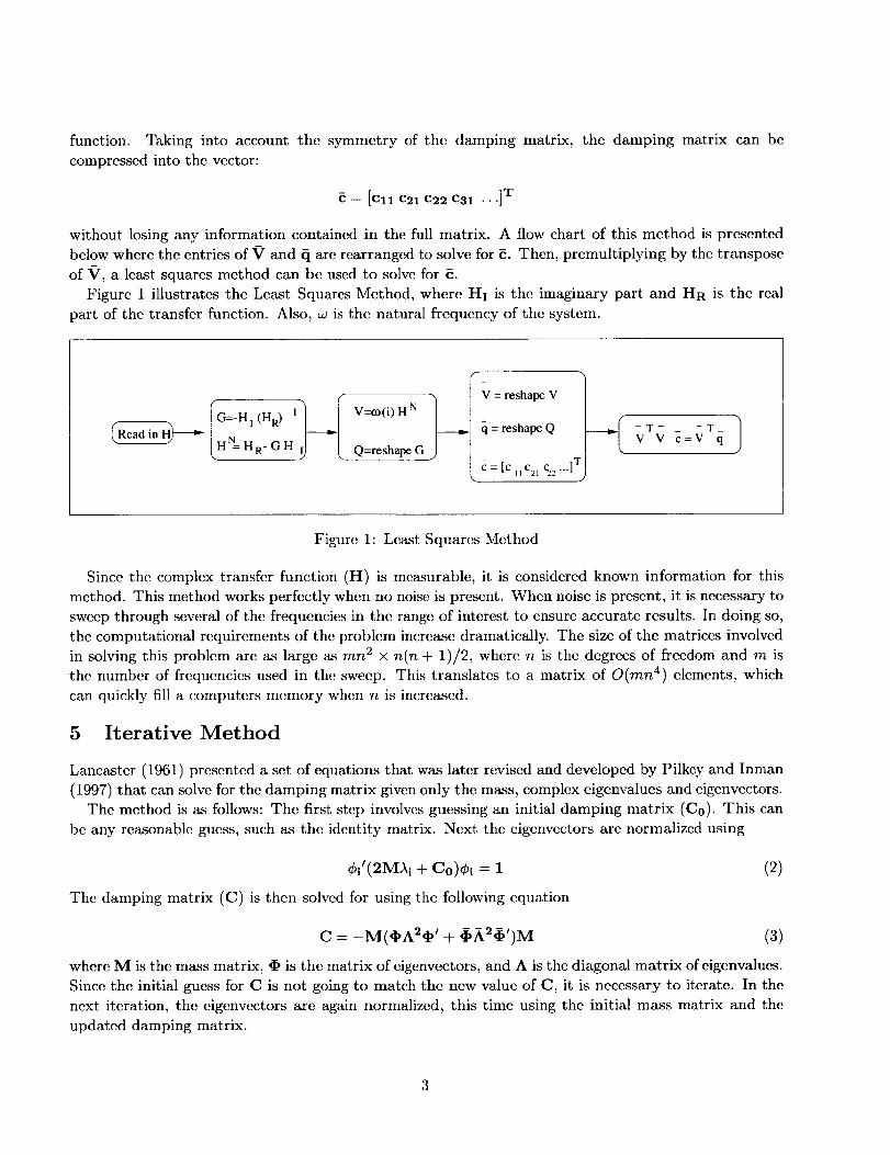
function. Taking into accountthe symmetryof the dampingmatrix, the damping matrix can becompressedinto the vector:

= [Cll e21 e22 e31 ...]T

without losing any information contained in the full matrix. A flow chart of this method is presented

below where the entries of V and Cl are rearranged to solve for _. Then, prcmultiplying by the transpose

of _r, a least squares method can be uscd to solve for _.

Figure 1 illustrates the Least Squares Method, where HI is the imaginary part and Ha is the real

part of the transfer function. Also, w is the natural frequency of the system.

G=_H l (HR) -1 V=¢o(i) H N

H N H R- G H Q=reshape G

V = reshape V

= reshape Q

c = [c ,1c21% ...]'r

-IvTV c=V q

Figure 1: Least Squares Mcthod

Since the complex transfer function (H) is measurable, it is considered known information for this

method. This method works perfectly when no noise is present. When noise is present, it is necessary to

sweep through several of the frequencies in the range of interest to ensure accurate results. In doing so,

the computational requirements of the problem increase dramatically. The size of the matrices involved

in solving this problcm arc as large as mn 2 x n(n + 1)//2, where n is the dcgrccs of freedom and m is

the number of frequencies used in the sweep. This translates to a matrix of O(rnn 4) elements, which

can quickly fill a computers memory when n is increased.

5 Iterative Method

Lancastcr (1961) prcscntcd a sct of equations that was later reviscd and developed by Pilkcy and Inman

(1997) that can solve for the damping matrix given only thc mass, complex eigenvalues and cigcnvectors.

Thc mcthod is as follows: The first step involvcs guessing an initial damping matrix (Co). This can

bc any rcasonablc guess, such as thc idcntity matrix. Ncxt the cigcnvcctors arc normalizcd using

¢i'(2MAi + Co)el = 1

The damping matrix (C) isthen solved for using the following equation

(2)

c = -M(OA2 ,' + 4 h2@')M (3)

where M is thc mass matrix, • is the matrix of cigcnvectors, and A is the diagonal matrix of cigenvalucs.

Since the initial guess for C is not going to match the ncw value of C, it is necessary to iterate. In the

next iteration, the cigcnvcctors are again normalized, this time using the initial mass matrix and the

updated damping matrix.

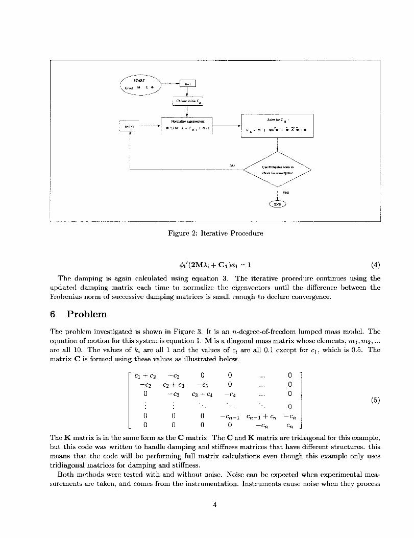
0'(2M _.+Cn. i ) _=1

r/ Solve fc¢ C _ :

lira/Ca=-M [ 0^20'+ 0 A_2_'IM

NO

Figure 2: Itcrative Procedure

¢il(2M)ki ÷ C1)¢i = 1 (4)

The damping is again calculated using equation 3. The iterative procedure continues using the

updated damping matrix each time to normalize the eigenvcctors until the difference between the

Frobcnius norm of successive damping matrices is small enough to dcclarc convergence.

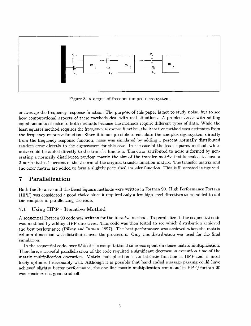
6 Problem

The problem investigated is shown in Figure 3. It is an n-degree-of-freedom lumpcd mass model. The

equation of motion for this system is equation 1. M is a diagonal mass matrix whose elements, ml, m2, ...

arc all 10. The values of ki arc all 1 and the values of ci arc all 0.1 except for Cl, which is 0.5. The

matrix C is formed using these values as illustrated below.

cl + c2 -c2 0 0 ... 0

-c2 c2 q- c3 -c3 0 ... 0

0 - c3 c3 if- c4 - c4 ... 0

: : ". "'. "'. 0

0 0 0 --C,n_1 C.n_1 q- Cn --C.n

0 0 0 0 -Cn ca

(5)

The K matrix is in the same form as the C matrix. The C and K matrix are tridiagonal for this example,

but this code was written to handle damping and stiffness matrices that have different structures, this

mcans that the code will bc pcrforming full matrix calculations cvcn though this example only uses

tridiagonal matrices for damping and stiffness.

Both methods were tested with and without noise. Noise can be expected when experimental mea-

surements arc taken, and comes from the instrumentation. Instruments cause noise when thcv process

4

C 2 C n

m

Figure 3: n degree-of-freedom lumped mass system

or average the frequency response function. The purpose of this paper is not to study noise, but to see

how computational aspects of these methods deal with real situations. A problem arose with adding

equal amounts of noise to both methods because the methods require different types of data. While the

least squares method requires the frequency response function, the iterativc method uses estimates from

the frequency response function. Since it is not possible to calculate the complex cigensystcm directly

from the frequency response function, noise was simulated by adding 1 percent normally distributed

random error directly to the eigensystem for this case. In the case of the least squares method, white

noise could bc added directly to the transfer function. The error attributed to noise is formed by gen-

erating a normally distributed random matrix the size of the transfer matrix that is scaled to have a

2-norm that is 1 percent of the 2-norm of the original transfer function matrix. The transfer matrix and

the error matrix arc added to form a slightly perturbed transfer function. This is illustrated in figure 4.

7 Parallelization

Both the Itcrativc and the Least Square methods were written in Fortran 90. High Performance Fortran

(HPF) was considered a good choice since it required only a few high level directives to bc added to aid

the compiler in parallelizing the code.

7.1 Using HPF - Iterative Method

A sequential Fortran 90 code was written for the itcrativc method. To parallclizc it, the sequential code

was modified by adding HPF directives. This code was then tested to see which distribution achieved

the best performance (Pilkcy and Inman, 1997). The best performance was achieved when the matrix

column dimension was distributed over the processors. Only this distribution was used for the final

simulation.

In the sequential code, over 95% of the computational time was spent on dense matrix multiplication.

Therefore, successful parallclization of the code required a significant deereasc in execution time of the

matrix multiplication operation. Matrix multiplication is an intrinsic function in HPF and is most

likely optimized reasonably well. Although it is possible that hand coded message passing could have

achieved slightly better performance, the one line matrix multiplication command in HPF/Fortran 90

was considered a good tradcoff.

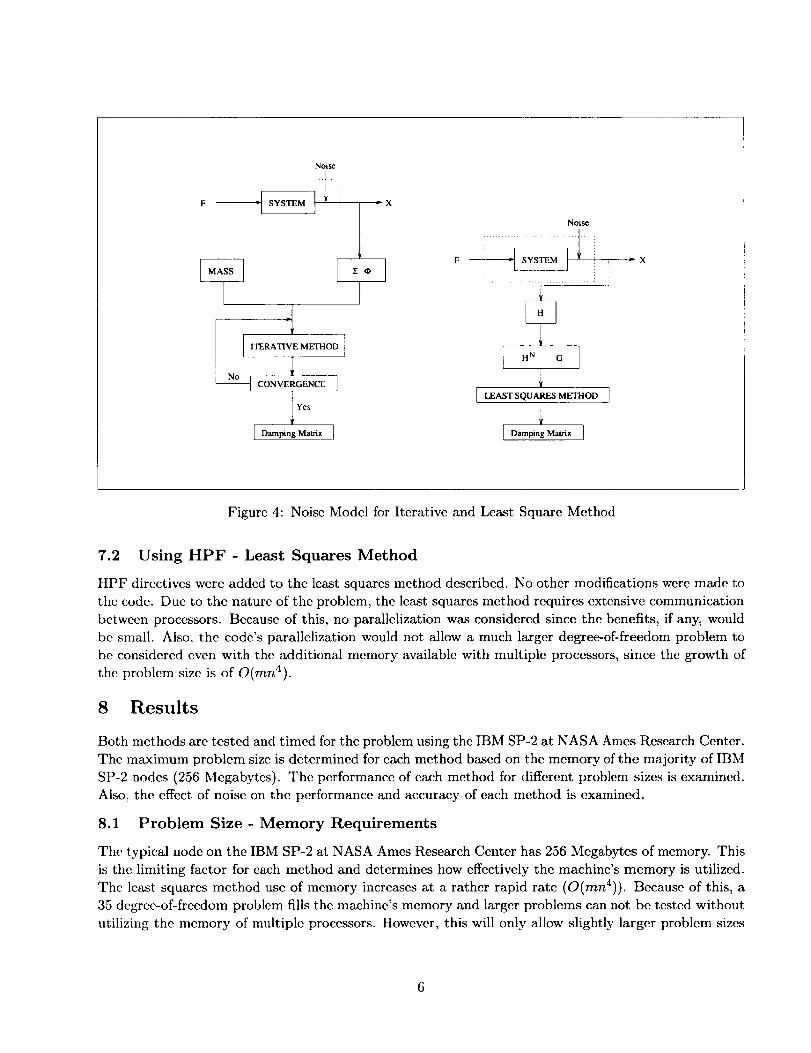
Noise

ITERATIVE METHOD

CONV SO . I

I Yes

[ Damping Matrix ]

Noise

H N G

I LEAST SQUARES METHOD

Figure 4: Noise Model for Iterative and Least Square Method

7.2 Using HPF - Least Squares Method

ItPF directives wcrc added to the least squares method described. No other modifications were made to

the code. Due to the nature of the problem, the least squares method requires extensive communication

between processors. Because of this, no paxallelization was considered since the benefits, if any, would

bc small. Also, the codc's parallelization would not allow a much larger degree-of-freedom problem to

bc considered even with the additional memory available with multiple processors, since the growth of

the problem size is of O(mna).

8 Results

Both methods are tested and timed for the problem using the IBM SP-2 at NASA Ames Research Center.

The maximum problem size is determined for each method based on the memory of the majority of IBM

SP-2 nodes (256 Megabytes). The performance of each method for different problem sizes is examined.

Also, the effect of noise on the performance and accuracy of each method is examined.

8.1 Problem Size - Memory Requirements

The typical node on the IBM SP-2 at NASA Ames Research Center has 256 Megabytes of memory. This

is the limiting factor for each method and determines how effectively the machine's memory is utilized.

The least squares method use of memory increases at a rather rapid rate (O(mn4)). Because of this, a

35 degree-of-freedom problem fills the machine's memory and larger problems can not be tested without

utilizing the memory of multiple processors. However, this will only allow slightly larger problem sizes

6

to betestedbecausethe amountof mcmoryavailablewill grow linearlywith the numberof processorsused,whilethe amountof memoryrequiredwill growat the rate O(mn4).

The iterativc mcthod is morc modest in its use of memory. Problem sizes ovcr 500 degrccs of freedom

can bc accommodated since the memory required will grow on the O(n2). The slower increase in memory

usage allows problcms with a high number of degrees of freedom to bc run on multiple processors.

8.2 Timing

Certain conventions were used in timing the results. First, 5-10 timings were taken for each test to

get an average since there were fluctuations in the timings on thc IBM SP-2. Sccond, only the actual

computation was timed; rcading the data files is not included in the timings. This was omitted becausc

it is inherently scqucntial and we have not currently cxamined parallel I/O. Future work may include

parallel I/O since the amount of time to read 500+ dcgrcc of freedom data scts can become significant.

Lastly, a fixed number of iterations was uscd to judge parallel spccdup. Although the problem may

have converged prior to the fixed number of iterations, the time required to reach the itcration number

appears in 2.

8.3 Performance

The problem was tested for many diffcrcnt degrees of freedom using both methods. Tests conducted

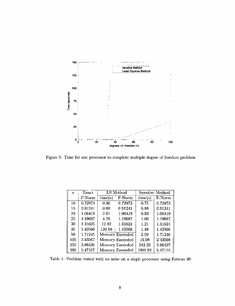
on the IBM SP-2 using sequential Fortran 90 arc prescntcd in Table 1 and Figure 5. Note that parallel

specdup refcrs to the p processor HPF time relative to thc one proccssor HPF time. Sequential speedup

refers to the p processor HPF time compaxcd to the sequential Fortran 90 time. The results show that

thc least squaxcs method is competitive with the itcrativc method up to 20 degrecs of freedom. After

that, the execution time increases at a much higher rate than the itcrativc method until it no longer fits

in mcmory. The maximum speedup obtained (Table 2) for: n = 100 is 1.70 using 4 processors, n = 250

is 3.79 for 8 processors, and n = 500 is 6.36 for 16 processors.

8.4 Error Associated with Noise

Calculations for accuracy and convergence wcrc made using the Frobenius norm, which is defined in

equation 6.

lICl'F = I _-_ _ 'ciJl2i--1 j--1 (6)

With this measure, both routines presented negligible crror without noise added to the system. When

1 pcrccnt noise is added (Table 3), the deviation from the exact known Frobenius norm for the iterativc

method ranges from 0.52% (for n = 500) to 0.83% (for n -- 20). The lcast squares routine did not

produce acceptable results when 1 pcrccnt noise was added to this problem for morc than 5 degrees of

freedom. Notice that there was vcry little change in cxccution time when the system with noise was

tcstcd. Because of this, thc parallel HPF timings wcrc almost identical to thc system without noise. In

addition, when the least squaxcs method was applied, the memory rcquirement increased. This is due to

the number (m) of additional frequencies nccdcd for accurate results. Correspondingly, only problems

with lower degrees of freedom axe able to fit in thc computer's memory.

9 Conclusions

Two methods for damping identification of an n degree-of-freedom lumped mass model have been

cxamincd. The least squares method has been shown to obtain the damping matrix for problems with

7

"o

.eb-

150 --

125

100

75

r

il Iterative Method /L Least Squares Metho d

50

J

25 j/J

Js_

0 0 20 40 60 80

degrees-of-freedom (n)

100

Figure 5: Time for one processor to complete multiple degree of freedom problem

n Exact

F-Norm

10 0.72973

15 0.91241

20 1.06419

25 1.19687

30 1.31625

35 1.42566

50 1.71245

100 2.43567

250 3.86426

5OO 5.471O7

LS Method Iterativc Method

time(s) F-Normtime(s) F-Norm0.36 0.72973

0.60 0.91241

2.61 1.06419

4.76 1.19687

12.92 1.31624

120.58 1.42566

Memory Exceeded

Memory Exceeded

Memory Exceeded

Memory Exceeded

0.75

0.88

0.93

1.06

1.21

1.48

2.59

16.08

243.32

1901.92

0.72973

0.91241

1.06419

1.19687

1.31624

1.42566

1.71246

2.43568

3.86427

5.47110

Table 1: Problem tested with no noise on a single processor using Fortran 90

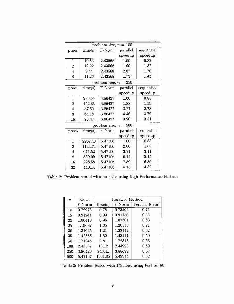
problemsize,n -- 100

procs time(s) F-Norm parallel sequential

speedup speedup

1 19.53

2 12.22

4 9.44

8 11.26

2.43568

2.43568

2.43568

2.43568

1.00

1.60

2.07

1.73

0.82

1.32

1.70

1.43

problem size, n = 250

procs time(s) F-Norm parallel sequential

speedup speedup

1 286.53

2 152.36

4 87.59

8 64.18

16 73.47

3.86427

3.86427

3.86427

3.86427

3.86427

1.00

1.88

3.27

4.46

3.90

0.85

1.59

2.78

3.79

3.31

problem size, n = 500

procs time(s) F-Norm parallel sequential

speedup speedup1 2267.43

2 1134.71

4 611.52

8 369.09

16 298.58

32 440.14

5.47106

5.47106

5.47106

5.47106

5.47106

5.47106

1.00

2.00

3.71

6.14

7.59

5.15

0.83

1.68

3.11

5.15

6.36

4.32

Table 2: Problem tested with no noise using High Pcrformanee Fortran

n Exact Itcrative Method

F-Norm time(s) F-Norm Percent Error10 0.72973

15 0.91241

20 1.06419

25 1.19687

30 1.31625

35 1.42566

50 1.71245

100 2.43567

250 3.86426

500 5.47107

0.78

0.90

0.96

1.05

1.21

1.52

2.81

16.12

243.41

1901.05

0.73492

0.91756

1.07301

1.20535

1.32442

1.43411

1.72318

2.44996

3.88629

5.49944

0.71

0.56

0.83

0.71

0.62

0.59

0.63

0.59

0.57

0.52

Table 3: Problem tested with 1% noise using Fortran 90

9

limited numbersof degrees-of-freedom.The least squaresmethodis restrictivebecauseof its largecomputermemoryrequirements.When1%noiseis addedto thesystem,the leastsquaresmethoddoesnot produceresultswith an acceptableamountof errorfor problemswith manydegreesof freedom.The iterativc methodis able to obtain the dampingmatrix for muchlarger problems. When 1%noiseis addcdto the system,the memoryrequirementof this methoddoesnot changeasin the leastsquaresmethod.In addition,a reasonablelevelof accuracyis maintainedwhennoiseis addedinto thesystem.Theiterativc methodalsorunswith a muchlowerexecutiontime. The only downsideto theitcrativemethodis that it maybcmoredifficult to applybecauseit requiresknowledgeof the complexcigcnvaluesand cigcnvcctors,while the leastsquaresmethodonly requiresknowlcdgcof the complextransferfunction.

Highperformancecomputing,specificallyparallelcomputing,maybebcncficialto theabovemethods.Forthe leastsquaresmethod,a largerdegree-of-freedomproblemmaybeexamined.However,becauseof the rapidly increasingmemoryrequirementof this methodthe bcncfit of parallelizationmay bemarginal. The bcnefitof usingparallelprocessorswith the iterative methodis muchgreaterfor tworeasons.If datais distributedamongmultipleprocessors,thenmuchlargerdegree-of-freedomproblemsmaybe examined.This meansthat problemswith over1000degreesof freedommaybc testable. Inthe future, methodsshouldbc devisedandexaminedfor scalabilityto ensurethat realisticproblemscanbc solved.

10 Acknowledgments

This work was done using the IBM SP-2 at NASA Langley Research Center and NASA Ames ResearchCenter.

The authors wish to acknowledge the support of the Virginia/ICASE/LaRC program in High Per-

formancc Computing. Support was also provided to the first author by the Virginia Space Grant

Consortium, and the first and last author by the Army Research Office

References

[1] Caravani, P., Thomson, W. T., 1974, "Identification of Damping Coefficients in Multidimensional

Linear Systems", ASME Journal of Applied Mechanics, Vol. 41, pp 379-382.

[2] Chert, S. Y., and Ju, M. S., and Tsuci, Y. G., 1996, "Estimation of Mass, Stiffness and Damping

Matrices from Frequency Response Functions", Journal of Vibration and Acoustics, Vol. 118, pp.78-82.

[3] Fritzcn, C.-P., 1986, "Identification of Mass, Damping, and Stiffness Matrices of Mechanical Sys-

tems', ASME Journal of Vibration, Acoustics, Stress, and Reliability in Design, Vol. 108, pp. 9-16.

[4] Hassclman, T.K., 1972, "A Method of Constructing a Full Modal Damping Matrix from Experi-

mental Measurements", AIAA Journal, Vol. 10, pp. 526-527.

[5] High Performance FORTRAN Forum. High Performance FORTRAN Language Specification, Ver-

sion 2.0, January 1997.

[6] Koclbcl, C.H., Lovcman, D.B., Schreibcr, R.S., Steele, C.L., Zosel, M.E., The High Performance

FORTRAN Handbook, The MIT Press, Cambridge, 1994.

10

[7] Lancaster,P. 1961,"Expressionfor DampingMatricesin LinearVibrationProblcm",Journal of the

Aerospace Sciences. pg. 256.

[8] Pilkey, D. F., Inman, D. J., 1997, "An Itcrativc Approach to Viscous Damping Matrix Idcntifica-

tion", Proceedings of the 15th International Modal Analysis Conference,

[9] Roemer, M. J., and Mook, D. J., 1992, "Mass, Stiffness, and Damping Matrix Identification: An

Intcgratcd Approach", ASME Journal of Vibration and Acoustics, Vol. 114, pp. 358-363.

11

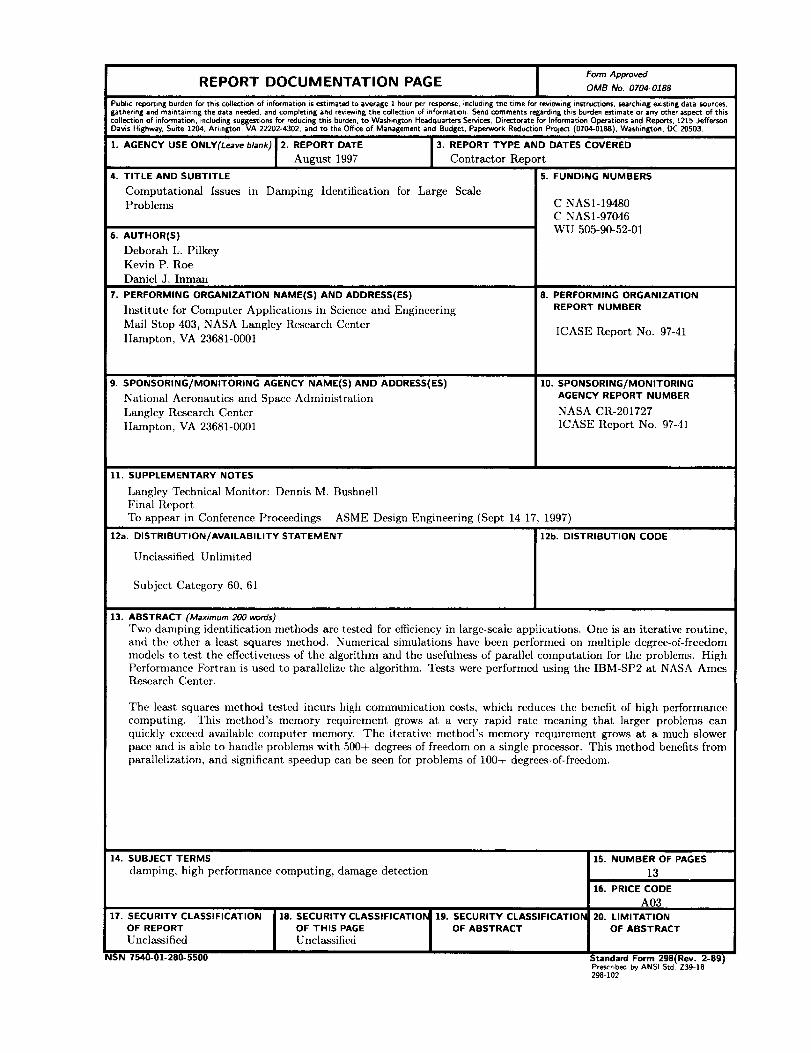
FormApprovedREPORT DOCUMENTATION PAGE OMB No. 0704-0188

Publicreportingburdenforthisco)lectionofinformationisestimatedto average1 hourperresponse,includingthetimeforreviewinginstructions,searchingexistingdatasources,gatheringandmaintainingthedataneeded,andcompletingandreviewingthecollectionofintrormationSendcommentsregardingthisburdenestimateor anyotheraspectofthiscollectionofinformation,includingsuggestionsfor reducingthisburden,to WashingtonHeadquartersServices,DirectorateforInformationOperationsandReports,1215JeffersonDavisHighway.Suite1204,Arlington.VA22202-4302,andto theOfficeof ManagementandBudget,Papen*_0rkReductionProJect(0704-0188l,Washington,DC20503.

1. AGENCY USE ONLY(Leaveblank) 2. REPORT DATE 3. REPORT TYPE AND DATES COVERED

August 1997 Contractor Report

4. TITLE AND SUBTITLE 5. FUNDING NUMBERS

Computational Issues in Damping Identification for Large ScaleProblems

6. AUTHOR(S)

Deborah L. PilkeyKevin P. Roe

Daniel J. Inman

7. PERFORMING ORGANIZATION NAME(S) AND ADDRESS(ES)

hlstitute for Computer Applications in Science and Engineering

Mail Stop 403, NASA Langley Research Center

Hampton, VA 23681-0001

9, SPONSORING/MONITORING AGENCY NAME(S) AND ADDRESS(ES)

National Aeronautics azld Space Administration

Langley Research Center

Hampton, VA 23681-0001

C NAS1-19480

C NAS1-97046WU 505-90-52-01

8. PERFORMING ORGANIZATIONREPORT NUMBER

ICASE Report No. 97-41

10. SPONSORING/MONITORINGAGENCY REPORT NUMBER

NASA CR-201727

ICASE Report No. 97-41

11. SUPPLEMENTARY NOTES

Langley Technical Monitor: Dennis M. Bushnell

FiIml Report

To appear in Conference Proceedings ASME Design Engineering (Sept 14-17, 1997)

12a. DISTRIBUTION/AVAILABILITY STATEMENT

Unclassified Unlimited

Subject Category 60, 61

12b. DISTRIBUTION CODE

13. ABSTRACT (Maximum200 words)Two damping identification methods are tested for efficiency in large-scale applications. One is an iterative routine,

and the other a least squares method. Numerical simulations have been performed on multiple degree-of-freedom

models to test the effectiveness of the algorithm and the usefulness of parallel computation for the problcn_s. High

Performance Fortran is used to parallclizc the algorithm. Tests were performed using the IBM-SP2 at NASA AmesResearch Center.

The least squares method tested incurs high communication costs, which reduces the benefit of high performance

computing. This method's memory requirement grows at a very rapid rate meaning that larger problems can

quickly exceed available computer memory. The itcrativc method's nlcmory requirement grows at a much slower

pace and is able to handle problems with 500+ degrees of freedom on a single processor. This method benefits from

parallelization, and significant speedup can bc seen for problems of 100+ degrees-of-freedom.

14. SUBJECT TERMSdamping, high performance computing, damage detection

17. SECURITY CLASSIFICATIONOF REPORTUnclassified

NSN 7540-01-280-5500

18. SECURITY CLASSIFICATION 19. SECURITY CLASSIFICATIONOF THIS PAGE OF ABSTRACTUnclassified

15. NUMBER OF PAGES

13

16. PRICE CODEA03

20. LIMITATIONOF ABSTRACT

Standard Form 298(Rev. 2-89)Prescrlbed by ANSI Std Z39-18298-102