1

MATHEMATICAL AND COMPUTATIONAL ISSUES IN CALCULATING CAPITAL FOR CREDIT RISK

Second Québec-Ontario Workshop on Insurance Mathematics February 3, 2012

David Saunders Department of Statistics and Actuarial Science University of Waterloo

Joint work with: J.C. Garcia-Cespedes, J.A. de Juan Herrero, A. Memartoluie, D. Rosen, and T. Wirjanto

2

Preface…

Counterparty risk is

“… probably the single most important variable in

determining whether and with what speed

financial disturbances become financial shocks,

with potential systemic traits”

Counterparty Risk Management Policy Group (CRMPG 2005)

3

Outline

1.  Credit Risk in the Trading Book

2.  Stress Testing CCR in the Basel Accord

3.  Worst Case Copulas: An Optimal Transportation

Problem

4.  Numerical Formulation

5.  Results

4

Risk in the Trading Book and Basel

Total Risk

Market risk Credit risk

- Equities - Commodities - Bonds and loans - OTC derivatives - Credit derivatives (CDSs, CDOs)

Portfolio VaR (e.g.10 days, 99%) - Includes spread risk

(specific risk)

5

Risk in the Trading Book and Basel

Total Risk

Market risk Credit risk Portfolio VaR (e.g.10 days, 99%)

- Includes spread risk (specific risk)

Stressed VaR (10 days, 99%) - Historical data from period of significant financial stress (e.g. 2007-2008).

6

Risk in the Trading Book and Basel

Total Risk

Credit risk 1. Counterparty credit risk

– derivatives including credit

– collateral, guarantees, mitigation

2. Issuer/borrower risk – bonds, loans, CDSs

3. Structured Credit – issuer/borrower + CP

Market risk

7

Risk in the Trading Book and Basel

Total Risk

Market risk Credit risk CreditVaR (Basel II - 1y, 99.9%)

•  Counterparty credit risk (CCR) - OTC derivatives, CDSs (CDOs)

•  Incremental risk charge (IRC) - Default, migration

-  Bonds, loans, CDSs •  Securitization (and correlation trading)

•  CVA VaR

8

Basel IRB Credit Capital Formula

  Basel II model: ASFM, heterogeneous portfolio, default and migration risk

€

Basel Capital = LGDj ⋅ EADj ⋅ ΦΦ−1 PDj( ) − ρ j Φ

−1 0.001( )1− ρ j

− PDj

⋅ MF M j ,PDj( )

j=1

N

∑

RWAs calculation relies on four quantitative inputs (risk components):

1.  Probability of default (PD): likelihood of borrower default over one year

2.  Exposure at default (EAD): amount that could be lost upon default

3.  Loss given default (LGD): proportion of exposure lost if default occurs

4.  Maturity (M): remaining economic maturity of the exposure

•  Another model parameter (set by the accord) is the asset correlation

9

Basel IRB Credit Capital Formula

  Basel II model: ASFM, heterogeneous portfolio, default and migration risk

€

Basel Capital = LGDj ⋅ EADj ⋅ ΦΦ−1 PDj( ) − ρ j Φ

−1 0.001( )1− ρ j

− PDj

⋅ MF M j ,PDj( )

j=1

N

∑

MF = maturity factor Captures “incremental” credit risk capital due to credit migration

(MF function calibrated by the BCBS)

Capital at 99.9% over one year - Default credit losses - Single-factor Merton-type model - Systematic risk (asymptotically fine-grained portfolio)

10

Basel and Potential Future Exposures (PFEs)

Source: de Prisco and Rosen (2005)

  Basel II – IRB credit capital   MtM + add-on internal models for EAD

11

  EPE and M computed from a counterparty Potential Future Exposure (PFE) simulation profile (including netting, collateral, etc.)

CCR and Basel – Internal Model

€

EAD =α ⋅Effective EPE

Expected Exposure (over all scenarios) at tk

Time-Averaged Exposure (for scenario s, up to time tk)

Expected Positive Exposure (EPE)

Effective Expected Exposure

Effective EPE

€

EE j (tk ) = PFE j (ωs,tk )pss=1

S

∑

€

µ jtk (ωs) = 1

tkPFE j (ωs,t)dt0

tk∫

€

EPE j (tk ) = 1tk

EE j (t)dt = µ jtk (ωs)ps

s=1

S

∑0

tk∫

€

µ jE (tk ) =max

0≤ i≤kEE j (tk )[ ] =max µ j

E (tk−1),EE j (tk )[ ]

€

Effective EPE j (tk ) = 1tk

µ jE (t)dt

0

tk∫

12

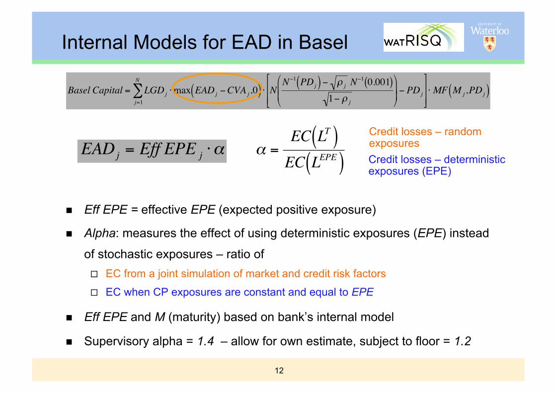
Internal Models for EAD in Basel

  Eff EPE = effective EPE (expected positive exposure)

  Alpha: measures the effect of using deterministic exposures (EPE) instead

of stochastic exposures – ratio of   EC from a joint simulation of market and credit risk factors

  EC when CP exposures are constant and equal to EPE

  Eff EPE and M (maturity) based on bank’s internal model

  Supervisory alpha = 1.4 – allow for own estimate, subject to floor = 1.2

€

Basel Capital = LGDj ⋅max EADj −CVA j ,0( ) ⋅ NN−1 PDj( ) − ρ j N

−1 0.001( )1− ρ j

− PDj

⋅ MF M j ,PDj( )

j=1

N

∑

€

α =EC LT( )EC LEPE( ) Credit losses – deterministic

exposures (EPE)

Credit losses – random exposures

€

EADj = Eff EPE j ⋅α

13

Summary – CCR Methodology (Garcia et al. 2010)   Computationally efficient approach CCR capital, alpha and CVA

  Leverages CP exposure simulations and preserves their joint distribution

  Can be applied within general integrated market-credit risk models   Simplified model that correlates (pre-computed) exposures with credit

factors leads to a parsimonious, computationally tractable approach   Consistent with the Basel model and also easy to implement

  Stress testing framework   Wrong-way risk and for risk management and regulatory applications   Numerical solution for inverse problem: finding the minimum level of

market-credit correlation which results in a floor for alpha (e.g. 1.2)   Stress test: market factors, correlations, exposures, time-steps

  Implemented and tested methodology at several international banks

14

CCR Capital – Correlated Market-Credit

General market-credit codependence framework

CP exposures (or market factors)

Capital

Copula Correlation parameters: ρ

Credit factors defaults

  Model: interpretable, auditable

  Empirical validation   Stress testing

15

Exposure Simulation

  Exposure scenarios are sorted in order of increasing time-averaged exposure, mapped to a normal.

  Regions between bars have equal probability.

!3 !2 !1 0 1 2 30

0.05

0.1

0.15

0.2

0.25

0.3

0.35

0.4

0.45

0.5

Y Value

PDF

1 2 3 4 S

16

Exposures

Sample portfolio: Approx. 2500 counterparties, 2000 market scenarios.

17

Stressed Exposures

18

Sorting Scenarios in Different Ways

19

Optimal Transportation Problem

  Is the method described above conservative?

  What is the “worst case copula”?

  Given:   XM : Market risk factors (exposures), with distribution PM

  XC : Credit risk factors, with distribution PC   Nonlinear loss function L(XM,XC).

  Risk Measure: ρ

  Solve:

€

maxΠ PM ,PC( )

ρ(L(XC ,XM ))

20

Related Work

  Bounds on Option Prices under Partial Information:   Bieglböck, Henry-Labodère and Penkner (2011), Galichon,

Henry-Labodère and Touzi (2010), Haase, Ilg, and Werner, 2010, Avellaneda, Levy, and Parás (1995), Tankov (2011).

  Risk Measures under Model Uncertainty: Cont (2006), Nutz and Soner (2010), Bion-Nadal and Kervarec (2010), Talay and Zheng (2002).

  Bounds on Distribution Functions and VaR: Embrechts and Puccetti (2006a,b), Puccetti and Rüschendorf (2011), Wang and Wang (2011).

21

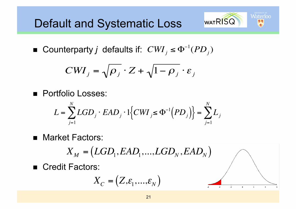
Default and Systematic Loss

  Counterparty j defaults if:

  Portfolio Losses:

  Market Factors:

  Credit Factors:

€

CWI j ≤ Φ−1(PDj )

€

CWI j = ρ j ⋅ Z + 1− ρ j ⋅ ε j

€

L = LGDj ⋅ EADj ⋅1 CWI j≤ Φ−1 PDj( ){ }

j=1

N

∑ = L jj=1

N

∑

€

XM = LGD1,EAD1,...,LGDN ,EADN( )

€

XC = Z,ε1,...,εN( )

22

Simplifications and Assumptions

  Use the existing exposure scenarios (from limits calculation) as the distribution of the market factors.   Resample for risk measurement calculations

  Only correlate systematic credit factors with market factors.   Use systematic losses in the optimal transportation problem.

  Discretize systematic credit factor distribution.

  Use CVaR as the risk measure (instead of VaR). €

LS = E L | Z[ ] = LGDj ⋅ EADj ⋅ ΦΦ−1(PDj ) − ρ j ⋅ Z

1− ρ j

j=1

N

∑

23

Optimization Problem   LGD adjusted exposure of CP j under market scenario m: yjm

  Marginal probabilities of market scenarios: πm   Marginal probabilities of credit scenarios:

  (Systematic) losses under a given market-credit scenario:

  Optimal transportation problem:

€

P(Z = Zs) = qs, s =1,...,S

€

Lms = y jm ⋅ ΦΦ−1(PDj ) − ρ j ⋅ Zs

1− ρ j

j=1

N

∑

€

maxp≥0

Risk p (L)

pms = qs, s =1,...,Sm=1

M∑

pms = πm, m =1,...,Ms=1

S∑

24

Optimization Problem

  Using CVaR, Rockafellar and Uryasev (2002), and a minimax theorem, the problem becomes:

  The inner (maximization) problem can be formulated as a linear program.

  The outer (minimization) problem is one-dimensional.

€

maxp≥0

minC

C +(1-α)-1 pms Lms −C( )+m,s∑

pms = qs, s =1,...,Sm=1

M∑

pms = πm, m =1,...,Ms=1

S∑

€

minC

maxp≥0

C +(1-α)-1 pms Lms −C( )+m,s∑

pms = qs, s =1,...,Sm=1

M∑

pms = πm , m =1,...,Ms=1

S∑

25

Optimal Transportation Problems

  Let and be prob. mass vectors

  be nonnegative matrix

  If is supermodular, i.e.,

for and

  We can find by the following greedy algorithm

26

Optimal Transportation Problems

  For a fixed C,

When exposures are monotonic, the supermodularity condition holds and we can use the previous greedy algo. to find the optimal joint distribution.

  Now if we solve this LP for the following value of parameters, we have:

€

maxp∈Π

C + (1−β)−1 pms Lms −C( )+m,s∑

Counterparties 10 10 10 10

Market Scenarios 1000 1000 1000 2000

Credit Scenarios 100 100 200 200 Confidence Level 0.95 0.95 0.95 0.95 GSS tolerance 0.05 0.025 0.025 0.05 CVaR 37.8286 38.2714 39.0033 40.4004

27

Algorithm

  Simulate from joint distribution of market factors and compute counterparty exposures.   Already carried out in practice for limits management

  Discretize systematic credit factors Z:

  Compute systematic losses under each combined market/credit scenario.

  Solve the worst-case copula optimal transportation problem.

  Sample from the resulting distribution to compute losses, risk measures, etc.

€

Z1 ≤ Z2 ≤ ≤ ZS

28

Example

  Portfolio of 50 counterparties, 2000 market scenarios.

0 5 10 15 20 25 30 35 40 45 500

2

4

6

8

10

12

14

16

18

0 5 10 15 20 25 30 35 40 45 500

2

4

6

8

10

12

14

5th percentile

mean

95th percentile

Counterparty

Counterparty

29

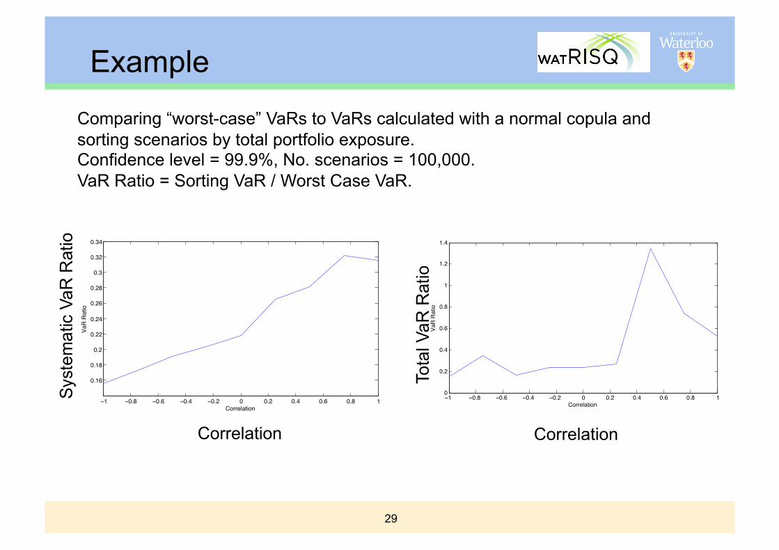
Example

Comparing “worst-case” VaRs to VaRs calculated with a normal copula and sorting scenarios by total portfolio exposure. Confidence level = 99.9%, No. scenarios = 100,000. VaR Ratio = Sorting VaR / Worst Case VaR.

!1 !0.8 !0.6 !0.4 !0.2 0 0.2 0.4 0.6 0.8 1

0.16

0.18

0.2

0.22

0.24

0.26

0.28

0.3

0.32

0.34

Correlation

Va

R R

atio

!1 !0.8 !0.6 !0.4 !0.2 0 0.2 0.4 0.6 0.8 10

0.2

0.4

0.6

0.8

1

1.2

1.4

Correlation

Va

R R

atio

Correlation Correlation

30

Future Work

  Importance sampling for the systematic credit factors.

  Accelerating computations through   Large scale optimization techniques   Exploitation of the structure of the LPs

  Convergence analysis of the discretized problems to the true optimal solution.   Error bounds

  Extensions to other problems in credit risk and risk management:   CVA, structured credit products,…

31

References

  Avellaneda, M., Levy, A., and Paràs, A., 1995, “Pricing and Hedging Derivatives Securities in Markets with Uncertain Volatilities”, Applied Mathematical Finance, 2, 73-88.

  Basel Committee on Banking Supervision, "International Convergence of Capital Measurements and Capital Standards: A Revised Framework, Comprehensive Version", 2006.

  Bieglböck, M., Henry-Labodère, P., and Penkner, F., 2011, “Model-Independent Bounds for Option Prices: A Mass Transportation Approach”, Working Paper.

  Bion-Nadal, J., and Kervarec, M., 2010, “Risk Measuring under Model Uncertainty”, Forthcoming in Annals of Applied Probability.

  E. Canabarro, E. Picoult and T. Wilde, "Analysing Counterparty Risk", Risk, 16(9), September, 2004.

  Cont, R., 2006, “Model Uncertainty and its Impact on the Pricing of Derivative Instruments”, Mathematical Finance, 16(3), 519-547.

  Counterparty Risk Management Policy Group, "Toward Greater Financial Stability: A Private Sector Perspective", 2005.

  B. de Prisco and D. Rosen, "Modelling Stochastic Counterparty Credit Exposures for Derivatives Portfolios", in "Counterparty Credit Risk Modelling", M. Pykhtin ed., Risk Books, 2005.

  Embrechts, P., and Puccetti, G., 2006a, “Bounds for Functions of Multivariate Risks”, Journal of Multivariate Analysis, 97, 526-547.

32

References

  Embrechts, P., and Puccetti., G, 2006b, Bounds for Functions of Dependent Risks”, Finance and Stochastics, 10, 341-352.

  Fleck, M. and Schmidt, A., 2005, “Analysis of Basel II Treatment of Counterparty Credit Risk”, Counterparty Credit Risk Modelling, M. Pykhtin Editor, Risk Books, London.

  Galichon A., Henry-Labodère, P., and Touzi, N., 2010, “A Stochastic Control Approach to No-Abitrage Bounds with Given Marginals, with an Application to Lookback Options”, Working Paper.

  Garcia Cespedes J. C., de Juan Herrero J. A., Rosen D., Saunders D. 2010, Effective modelling of Wrong-Way Risk, CCR Capital, and Alpha in Basel II”, Journal of Risk Model Validation, 4(1), pages 71-98.

  Glasserman, P., and Yao, D.D., 2004, “Optimal Couplings are Totally Positive and More”, Journal of Applied Probability, 41A, 321-332.

  Haase, J, Ilg, M., and Werner, R., 2010, “Model-Free Bounds on Bilateral Counterparty Valuation”, Working Paper.

  Nutz, M., and Soner, H.M., 2010, “Superhedging and Dynamic Risk Measures under Model Uncertainty”, Working Paper.

  E. Picoult, “Calculating and Hedging Exposure, Credit Value Adjustment and Economic Capital for Counterparty Credit Risk”, in "Counterparty Credit Risk Modelling", M. Pykhtin ed., Risk Books, 2005.

33

References

  Puccetti, G., and Rüschendorf, 2011, “Bounds for Joint Portfolios of Dependent Risks”, Working Paper.

  Rockafellar, R.T., and Uryasev, S., 2002, “Conditional value-at-risk for general loss distributions”, Journal of Banking & Finance, 26, 1443-1471.

  Rosen D. and Saunders D. 2010, Computing and Stress Testing Counterparty Credit Risk Capital, in Counterparty Credit Risk Modelling, (ed. E. Canabarro), Risk Books.

  Talay, D., and Zheng, Z., 2002, “Worst Case Model Risk Management”, Finance and Stochastics, 6, 517-537.

  Tankov, P., 2011, “Improved Frechet Bounds and Model-Free Pricing of Multi-Asset Options”, Journal of Applied Probability, 43, 389-403.

  Wang, B., and Wang, R., 2011, “The Complete Mixability and Convex Minimization Problems with Monotone Marginal Densities”, Forthcoming in Journal of Multivariate Analysis.