Embed Size (px)
Citation preview
User Manual
COMPUTATIONAL INFRASTRUCTURE FOR GEODYNAMICS (CIG)
Version 7.0
PRINCETON UNIVERSITY (USA)CNRS and UNIVERSITY OF MARSEILLE (FRANCE)
SPECFEM 2D
SPECFEM2DUser Manual
© Princeton University (USA) and CNRS / University of Marseille (France)Version 7.0
January 20, 2015

1
AuthorsThe SPECFEM2D package was first developed by Dimitri Komatitsch and Jean-Pierre Vilotte at IPG in Paris (France)from 1995 to 1997 and then by Dimitri Komatitsch at Harvard University (USA), Caltech (USA) and then CNRS andUniversity of Pau (France) from 1998 to 2005. The story started on April 4, 1995, when Prof. Yvon Maday fromCNRS and University of Paris, France, gave a lecture to Dimitri Komatitsch and Jean-Pierre Vilotte at IPG aboutthe nice properties of the Legendre spectral-element method with diagonal mass matrix that he had used for otherequations. We are deeply indebted and thankful to him for that. That followed a visit by Dimitri Komatitsch to OGS(Istituto Nazionale di Oceanografia e di Geofisica Sperimentale) in Trieste, Italy, in February 1995 to meet with GézaSeriani and Enrico Priolo, who introduced him to their 2D Chebyshev version of the spectral-element method with anon-diagonal mass matrix. We are deeply indebted and thankful to them for that.
Since then it has been developed and maintained by a development team: in alphabetical order, Paul Cristini, Dim-itri Komatitsch, Jesús Labarta, Nicolas Le Goff, Pieyre Le Loher, Qinya Liu, Roland Martin, René Matzen, ChristinaMorency, Daniel Peter, Carl Tape, Jeroen Tromp, Jean-Pierre Vilotte, Zhinan Xie.
The code is released open-source under the CeCILL version 2 license, see the license at the end of this manual.

2
Current and past main participants or main sponsors (in no particular order)
Contents
Contents 3
1 Introduction 41.1 Citation . . . . . . . . . . . . . . . . . . . . . . . . . . . . . . . . . . . . . . . . . . . . . . . . . . 51.2 Support . . . . . . . . . . . . . . . . . . . . . . . . . . . . . . . . . . . . . . . . . . . . . . . . . . 6
2 Getting Started 72.1 Visualizing the subroutine calling tree of the source code . . . . . . . . . . . . . . . . . . . . . . . . 82.2 Becoming a developer of the code, or making small modifications in the source code . . . . . . . . . 8
3 Mesh Generation 93.1 How to use SPECFEM2D . . . . . . . . . . . . . . . . . . . . . . . . . . . . . . . . . . . . . . . . . 93.2 How to use Gmsh to generate an external mesh . . . . . . . . . . . . . . . . . . . . . . . . . . . . . 113.3 Controlling the quality of an external mesh . . . . . . . . . . . . . . . . . . . . . . . . . . . . . . . 133.4 Controlling how the mesh samples the wave field . . . . . . . . . . . . . . . . . . . . . . . . . . . . 13
4 Running the Solver xspecfem2D 144.1 How to run P-SV or SH (membrane) wave simulations . . . . . . . . . . . . . . . . . . . . . . . . . 174.2 How to use anisotropy . . . . . . . . . . . . . . . . . . . . . . . . . . . . . . . . . . . . . . . . . . 174.3 How to use poroelasticity . . . . . . . . . . . . . . . . . . . . . . . . . . . . . . . . . . . . . . . . . 174.4 How to set plane waves as initial conditions . . . . . . . . . . . . . . . . . . . . . . . . . . . . . . . 194.5 How to choose the time step . . . . . . . . . . . . . . . . . . . . . . . . . . . . . . . . . . . . . . . 19
5 Adjoint Simulations 215.1 How to obtain Finite Sensitivity Kernels . . . . . . . . . . . . . . . . . . . . . . . . . . . . . . . . . 215.2 Remarks about adjoint runs and solving inverse problems . . . . . . . . . . . . . . . . . . . . . . . . 225.3 Caution . . . . . . . . . . . . . . . . . . . . . . . . . . . . . . . . . . . . . . . . . . . . . . . . . . 22
6 Oil and gas industry simulations 23
Bibliography 26
A Troubleshooting 32
B License 33
3
Chapter 1
Introduction
SPECFEM2D facilitates 2D simulations of acoustic, (an)elastic, and poroelastic seismic wave propagation. The 2Dspectral-element solver accommodates regular and unstructured meshes, generated for example by Cubit (http://cubit.sandia.gov), Gmsh (http://geuz.org/gmsh) or GiD (http://www.gid.cimne.upc.es).Even mesh creation packages that generate triangles, for instance Delaunay-Voronoi triangulation codes, can be usedbecause each triangle can then easily be decomposed into three quadrangles by linking the barycenter to the center ofeach edge; while this approach does not generate quadrangles of optimal quality, it can ease mesh creation in somesituations and it has been shown that the spectral-element method can very accurately handle distorted mesh elements.
With version 7.0, the 2D spectral-element solver accommodates Convolution PML absorbing layers and well ashigher-order time schemes (4th order Runge-Kutta and LDDRK4-6). Convolution or Auxiliary Differential EquationPerfectly Matched absorbing Layers (C-PML or ADE-PML) are described in Martin et al. [2008b,c], Martin andKomatitsch [2009], Martin et al. [2010], Komatitsch and Martin [2007].
The solver has adjoint capabilities and can calculate finite-frequency sensitivity kernels [Tromp et al., 2008, Peteret al., 2011] for acoustic, (an)elastic, and poroelastic media. The package also considers 2D SH and P-SV wave propa-gation. Finally, the solver can run both in serial and in parallel. See SPECFEM2D (http://www.geodynamics.org/cig/software/packages/seismo/specfem2d) for the source code.
The SEM is a continuous Galerkin technique [Tromp et al., 2008, Peter et al., 2011], which can easily be made dis-continuous [Bernardi et al., 1994, Chaljub, 2000, Kopriva et al., 2002, Chaljub et al., 2003, Legay et al., 2005, Kopriva,2006, Wilcox et al., 2010, Acosta Minolia and Kopriva, 2011]; it is then close to a particular case of the discontinuousGalerkin technique [Reed and Hill, 1973, Lesaint and Raviart, 1974, Arnold, 1982, Johnson and Pitkäranta, 1986,Bourdel et al., 1991, Falk and Richter, 1999, Hu et al., 1999, Cockburn et al., 2000, Giraldo et al., 2002, Rivière andWheeler, 2003, Monk and Richter, 2005, Grote et al., 2006, Ainsworth et al., 2006, Bernacki et al., 2006, Dumbser andKäser, 2006, De Basabe et al., 2008, de la Puente et al., 2009, Wilcox et al., 2010, De Basabe and Sen, 2010, Étienneet al., 2010], with optimized efficiency because of its tensorized basis functions [Wilcox et al., 2010, Acosta Minoliaand Kopriva, 2011]. In particular, it can accurately handle very distorted mesh elements [Oliveira and Seriani, 2011].
It has very good accuracy and convergence properties [Maday and Patera, 1989, Seriani and Priolo, 1994, Devilleet al., 2002, Cohen, 2002, De Basabe and Sen, 2007, Seriani and Oliveira, 2008, Ainsworth and Wajid, 2009, 2010,Melvin et al., 2012]. The spectral element approach admits spectral rates of convergence and allows exploiting hp-convergence schemes. It is also very well suited to parallel implementation on very large supercomputers [Komatitschet al., 2003, Tsuboi et al., 2003, Komatitsch et al., 2008, Carrington et al., 2008, Komatitsch et al., 2010b] as well ason clusters of GPU accelerating graphics cards [Komatitsch, 2011, Michéa and Komatitsch, 2010, Komatitsch et al.,2009, 2010a]. Tensor products inside each element can be optimized to reach very high efficiency [Deville et al.,2002], and mesh point and element numbering can be optimized to reduce processor cache misses and improve cachereuse [Komatitsch et al., 2008]. The SEM can also handle triangular (in 2D) or tetrahedral (in 3D) elements [Wingateand Boyd, 1996, Taylor and Wingate, 2000, Komatitsch et al., 2001, Cohen, 2002, Mercerat et al., 2006] as well asmixed meshes, although with increased cost and reduced accuracy in these elements, as in the discontinuous Galerkinmethod.
Note that in many geological models in the context of seismic wave propagation studies (except for instance forfault dynamic rupture studies, in which very high frequencies or supershear rupture need to be modeled near the fault,see e.g. Benjemaa et al. [2007, 2009], de la Puente et al. [2009], Tago et al. [2010]) a continuous formulation is
4
CHAPTER 1. INTRODUCTION 5
sufficient because material property contrasts are not drastic and thus conforming mesh doubling bricks can efficientlyhandle mesh size variations [Komatitsch and Tromp, 2002, Komatitsch et al., 2004, Lee et al., 2008, 2009a,b].
For a detailed introduction to the SEM as applied to regional seismic wave propagation, please consult Peter et al.[2011], Tromp et al. [2008], Komatitsch and Vilotte [1998], Komatitsch and Tromp [1999], Chaljub et al. [2007] andin particular Lee et al. [2009b,a, 2008], Godinho et al. [2009], van Wijk et al. [2004], Komatitsch et al. [2004]. Adetailed theoretical analysis of the dispersion and stability properties of the SEM is available in Cohen [2002], DeBasabe and Sen [2007], Seriani and Oliveira [2007], Seriani and Oliveira [2008] and Melvin et al. [2012].
The SEM was originally developed in computational fluid dynamics [Patera, 1984, Maday and Patera, 1989] andhas been successfully adapted to address problems in seismic wave propagation. Early seismic wave propagationapplications of the SEM, utilizing Legendre basis functions and a perfectly diagonal mass matrix, include Cohen et al.[1993], Komatitsch [1997], Faccioli et al. [1997], Casadei and Gabellini [1997], Komatitsch and Vilotte [1998] andKomatitsch and Tromp [1999], whereas applications involving Chebyshev basis functions and a non-diagonal massmatrix include Seriani and Priolo [1994], Priolo et al. [1994] and Seriani et al. [1995].
All SPECFEM2D software is written in Fortran2003 with full portability in mind, and conforms strictly to theFortran2003 standard. It uses no obsolete or obsolescent features of Fortran. The package uses parallel programmingbased upon the Message Passing Interface (MPI) [Gropp et al., 1994, Pacheco, 1997].
The next release of the code will include support for GPU graphics card acceleration [Komatitsch, 2011, Michéaand Komatitsch, 2010, Komatitsch et al., 2009, 2010a].
The code uses the plane strain convention when the standard P-SV equation case is used, i.e., the off-plane strainεzz is zero by definition of the plane strain convention but the off-plane stress σzz is not equal to zero, one hasσzz = λ(εxx+εyy). This implies, as in any plain strain software package, that the P-SV source is a line source along thedirection perpendicular to the plane (see file discussion_of_2D_sources_and_approximations_from_Pilant_1979.pdffor more details).
1.1 CitationIf you use this code for your own research, please cite at least one article written by the developers of the package, forinstance:
• Tromp et al. [2008],
• Peter et al. [2011],
• Vai et al. [1999],
• Lee et al. [2009a],
• Lee et al. [2008],
• Lee et al. [2009b],
• Komatitsch et al. [2010a],
• Komatitsch et al. [2009],
• Liu et al. [2004],
• Chaljub et al. [2007],
• Komatitsch and Vilotte [1998],
• Komatitsch and Tromp [1999],
• Komatitsch et al. [2004],
• Morency and Tromp [2008],
• and/or other articles from http://komatitsch.free.fr/publications.html.
CHAPTER 1. INTRODUCTION 6
If you use the kernel capabilities of the code, please cite at least one article written by the developers of the package,for instance:
• Tromp et al. [2008],
• Peter et al. [2011],
• Liu and Tromp [2006],
• Morency et al. [2009].
If you use the SCOTCH / CUBIT non-structured capabilities, please also cite:
• Martin et al. [2008a].
The corresponding BibTEX entries may be found in file doc/USER_MANUAL/bibliography.bib.
1.2 SupportThis material is based upon work supported by the USA National Science Foundation under Grants No. EAR-0406751and EAR-0711177, by the French CNRS, French Inria Sud-Ouest MAGIQUE-3D, French ANR NUMASIS underGrant No. ANR-05-CIGC-002, and European FP6 Marie Curie International Reintegration Grant No. MIRG-CT-2005-017461. Any opinions, findings, and conclusions or recommendations expressed in this material are those of theauthors and do not necessarily reflect the views of the USA National Science Foundation, CNRS, Inria, ANR or theEuropean Marie Curie program.
Chapter 2
Getting Started
To download the SPECFEM2D software package, type this:
git clone --recursive --branch devel https://github.com/geodynamics/specfem2d.git
We recommend that you add ulimit -S -s unlimited to your .bash_profile file and/or limitstacksize unlimited to your .cshrc file to suppress any potential limit to the size of the Unix stack.
Then, to configure the software for your system, run the configure shell script. This script will attempt to guessthe appropriate configuration values for your system. However, at a minimum, it is recommended that you explicitlyspecify the appropriate command names for your Fortran compiler (another option is to define FC, CC and MPIF90 inyour .bash_profile or your .cshrc file):
./configure FC=ifort
If you want to run in parallel, i.e., using more than one processor core, then you would type
./configure FC=ifort MPIFC=mpif90 --with-mpi
Before running the configure script, you should probably edit file flags.guess to make sure that it containsthe best compiler options for your system. Known issues or things to check are:
Intel ifort compiler See if you need to add -assume byterecl for your machine. In the case of thatcompiler, we have noticed that versions dot zero sometimes have bugs or issues that can lead to wrongresults when running the code, thus we strongly recommend using versions dot one or above (for instanceversion 13.1 instead of 13.0, version 14.1 instead of 14.0 and so on).
IBM compiler See if you need to add -qsave or -qnosave for your machine.
Mac OS You will probably need to install XCODE.
IBM Blue Gene machines Please refer to the manual of SPECFEM3D_Cartesian, which contains detailed in-structions on how to run on Blue Gene.
The SPECFEM2D software package relies on the SCOTCH library to partition meshes. The SCOTCH library[Pellegrini and Roman, 1996] provides efficient static mapping, graph and mesh partitioning routines. SCOTCH is afree software package developed by François Pellegrini et al. from LaBRI and Inria in Bordeaux, France, download-able from the web page https://gforge.inria.fr/projects/scotch/. In case no SCOTCH librariescan be found on the system, the configuration will bundle the version provided with the source code for compilation.The path to an existing SCOTCH installation can to be set explicitly with the option --with-scotch-dir. Just asan example:
./configure FC=ifort MPIFC=mpif90 --with-mpi --with-scotch-dir=/opt/scotch
If you use the Intel ifort compiler to compile the code, we recommend that you use the Intel icc C compiler to compileScotch, i.e., use:
7
CHAPTER 2. GETTING STARTED 8
./configure CC=icc FC=ifort MPIFC=mpif90
For further details about the installation of SCOTCH, go to subdirectory scotch_5.1.11/ and read INSTALL.txt.You may want to download more recent versions of SCOTCH in the future from (http://www.labri.fr/perso/pelegrin/scotch/scotch_en.html) . Support for the METIS graph partitioner has been discon-tinued because SCOTCH is more recent and performs better.
When compiling the SCOTCH source code, if you get a message such as: "ld: cannot find -lz", the Zlib com-pression development library is probably missing on your machine and you will need to install it or ask your systemadministrator to do so. On Linux machines the package is often called "zlib1g-dev" or similar. (thus "sudo apt-getinstall zlib1g-dev" would install it)
You may edit the Makefile for more specific modifications. Especially, there are several options available:
• -DUSE_MPI compiles with use of an MPI library.
• -DUSE_SCOTCH enables use of graph partitioner SCOTCH.
After these steps, go back to the main directory of SPECFEM2D/ and type
make
to create all executables which will be placed into the folder ./bin/.By default, the solver runs in single precision. This is fine for most application, but if for some reason you want
to run the solver in double precision, run the configure script with option “--enable-double-precision”.Keep in mind that this will of course double total memory size and will also make the solver around 20 to 30% sloweron many processors.
If your compiler has problems with the use mpi statements that are used in the code, use the script calledreplace_use_mpi_with_include_mpif_dot_h.pl in the root directory to replace all of them with include‘mpif.h’ automatically.
2.1 Visualizing the subroutine calling tree of the source codePackages such as doxywizard can be used to visualize the subroutine calling tree of the source code. Doxywizardis a GUI front-end for configuring and running doxygen.
2.2 Becoming a developer of the code, or making small modifications in thesource code
If you want to develop new features in the code, and/or if you want to make small changes, improvements, or bugfixes, you are very welcome to contribute. To do so, i.e. to access the development branch of the source code withread/write access (in a safe way, no need to worry too much about breaking the package, there is a robot calledBuildBot that is in charge of checking and validating all new contributions and changes), please visit this Web page:https://github.com/geodynamics/specfem2d/wiki/Using-Hub.
Chapter 3
Mesh Generation
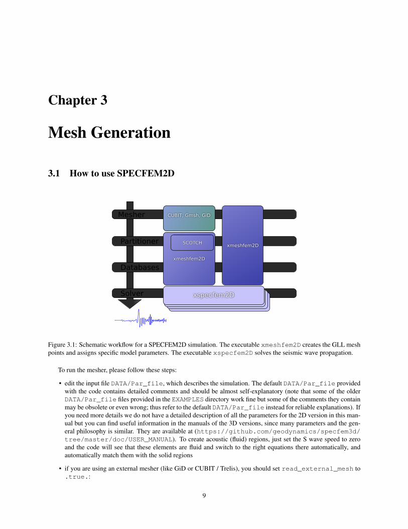
3.1 How to use SPECFEM2D
Mesher
Partitioner
Databases
Solver
CUBIT, Gmsh, GiD
SCOTCH
xmeshfem2D
xmeshfem2D
xspecfem2D
Figure 3.1: Schematic workflow for a SPECFEM2D simulation. The executable xmeshfem2D creates the GLL meshpoints and assigns specific model parameters. The executable xspecfem2D solves the seismic wave propagation.
To run the mesher, please follow these steps:
• edit the input file DATA/Par_file, which describes the simulation. The default DATA/Par_file providedwith the code contains detailed comments and should be almost self-explanatory (note that some of the olderDATA/Par_file files provided in the EXAMPLES directory work fine but some of the comments they containmay be obsolete or even wrong; thus refer to the default DATA/Par_file instead for reliable explanations). Ifyou need more details we do not have a detailed description of all the parameters for the 2D version in this man-ual but you can find useful information in the manuals of the 3D versions, since many parameters and the gen-eral philosophy is similar. They are available at (https://github.com/geodynamics/specfem3d/tree/master/doc/USER_MANUAL). To create acoustic (fluid) regions, just set the S wave speed to zeroand the code will see that these elements are fluid and switch to the right equations there automatically, andautomatically match them with the solid regions
• if you are using an external mesher (like GiD or CUBIT / Trelis), you should set read_external_mesh to.true.:
9
CHAPTER 3. MESH GENERATION 10
mesh_file is the file describing the mesh : first line is the number of elements, then a list of 4 nodes (quadri-laterals only) forming each elements on each line.
nodes_coords_file is the file containing the coordinates (x and z) of each node: number of nodes on thefirst line, then coordinates x and z on each line.
materials_file is the number of the material for every element : an integer ranging from 1 to nbmodelson each line.
free_surface_file is the file describing the edges forming the acoustic free surface: number of edges onthe first line, then on each line: number of the element, number of nodes forming the free surface (1 fora point, 2 for an edge), the nodes forming the free surface for this element. If you do not want any freesurface, just put 0 on the first line.
absorbing_surface_file is the file describing the edges forming the absorbing boundaries: number ofedges on the first line, then on each line: number of the element, number of nodes forming the absorbingedge (must always be equal to 2), the two nodes forming the absorbing edge for this element, and then thetype of absorbing edge: 1 for BOTTOM, 2 for RIGHT, 3 for TOP and 4 for LEFT. Only two nodes perelement can be listed, i.e., the second parameter of each line must always be equal to 2. If one of yourelements has more than one edge along a given absorbing contour (e.g., if that contour has a corner) thenlist it twice, putting the first edge on the first line and the second edge on the second line. Do not listthe same element with the same absorbing edge twice or more, otherwise absorption will not be correctbecause the edge integral will be improperly subtracted several times. If one of your elements has a singlepoint along the absorbing contour rather than a full edge, do NOT list it (it would have no weight in thecontour integral anyway because it would consist of a single point). If you use 9-node elements, list onlythe first and last points of the edge and not the intermediate point located around the middle of the edge;the right 9-node curvature will be restored automatically by the code.
tangential_detection_curve_file contains points describing the envelope, that are used for thesource_normal_to_surface and rec_normal_to_surface. Should be fine grained, and or-dered clockwise. Number of points on the first line, then (x,z) coordinates on each line.
• if you have compiled with MPI, you must specify the number of processes.
Then type
./bin/xmeshfem2D
to create the mesh (which will be stored in directory OUTPUT_FILES/). xmeshfem2D is serial; it will outputseveral files called Database??????, one for each process.
0
500
1000
1500
2000
2500
3000
3500
0 500 1000 1500 2000 2500 3000 3500 4000
'OUTPUT_FILES.default.M2_UPPA/gridfile.gnu'
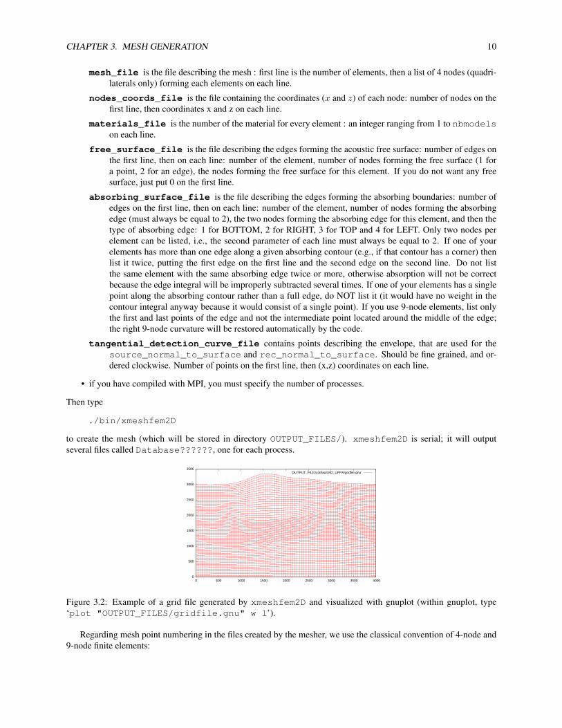
Figure 3.2: Example of a grid file generated by xmeshfem2D and visualized with gnuplot (within gnuplot, type‘plot "OUTPUT_FILES/gridfile.gnu" w l’).
Regarding mesh point numbering in the files created by the mesher, we use the classical convention of 4-node and9-node finite elements:
CHAPTER 3. MESH GENERATION 11
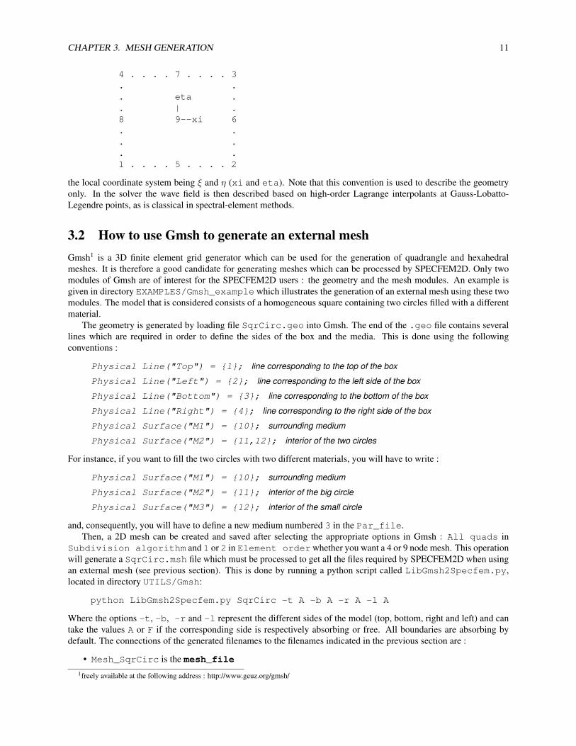
4 . . . . 7 . . . . 3. .. eta .. | .8 9--xi 6. .. .. .1 . . . . 5 . . . . 2
the local coordinate system being ξ and η (xi and eta). Note that this convention is used to describe the geometryonly. In the solver the wave field is then described based on high-order Lagrange interpolants at Gauss-Lobatto-Legendre points, as is classical in spectral-element methods.
3.2 How to use Gmsh to generate an external meshGmsh1 is a 3D finite element grid generator which can be used for the generation of quadrangle and hexahedralmeshes. It is therefore a good candidate for generating meshes which can be processed by SPECFEM2D. Only twomodules of Gmsh are of interest for the SPECFEM2D users : the geometry and the mesh modules. An example isgiven in directory EXAMPLES/Gmsh_example which illustrates the generation of an external mesh using these twomodules. The model that is considered consists of a homogeneous square containing two circles filled with a differentmaterial.
The geometry is generated by loading file SqrCirc.geo into Gmsh. The end of the .geo file contains severallines which are required in order to define the sides of the box and the media. This is done using the followingconventions :
Physical Line("Top") = {1}; line corresponding to the top of the box
Physical Line("Left") = {2}; line corresponding to the left side of the box
Physical Line("Bottom") = {3}; line corresponding to the bottom of the box
Physical Line("Right") = {4}; line corresponding to the right side of the box
Physical Surface("M1") = {10}; surrounding medium
Physical Surface("M2") = {11,12}; interior of the two circles
For instance, if you want to fill the two circles with two different materials, you will have to write :
Physical Surface("M1") = {10}; surrounding medium
Physical Surface("M2") = {11}; interior of the big circle
Physical Surface("M3") = {12}; interior of the small circle
and, consequently, you will have to define a new medium numbered 3 in the Par_file.Then, a 2D mesh can be created and saved after selecting the appropriate options in Gmsh : All quads in
Subdivision algorithm and 1 or 2 in Element orderwhether you want a 4 or 9 node mesh. This operationwill generate a SqrCirc.msh file which must be processed to get all the files required by SPECFEM2D when usingan external mesh (see previous section). This is done by running a python script called LibGmsh2Specfem.py,located in directory UTILS/Gmsh:
python LibGmsh2Specfem.py SqrCirc -t A -b A -r A -l A
Where the options -t, -b, -r and -l represent the different sides of the model (top, bottom, right and left) and cantake the values A or F if the corresponding side is respectively absorbing or free. All boundaries are absorbing bydefault. The connections of the generated filenames to the filenames indicated in the previous section are :
• Mesh_SqrCirc is the mesh_file1freely available at the following address : http://www.geuz.org/gmsh/
CHAPTER 3. MESH GENERATION 12
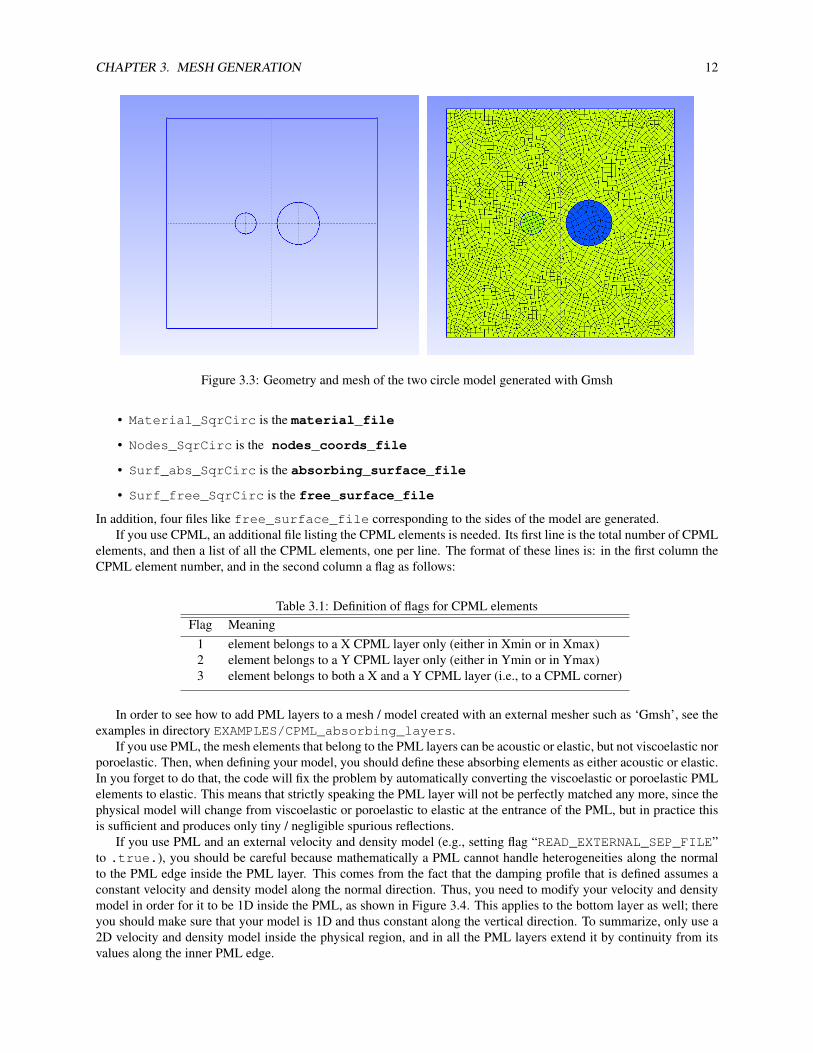
Figure 3.3: Geometry and mesh of the two circle model generated with Gmsh
• Material_SqrCirc is the material_file
• Nodes_SqrCirc is the nodes_coords_file
• Surf_abs_SqrCirc is the absorbing_surface_file
• Surf_free_SqrCirc is the free_surface_file
In addition, four files like free_surface_file corresponding to the sides of the model are generated.If you use CPML, an additional file listing the CPML elements is needed. Its first line is the total number of CPML
elements, and then a list of all the CPML elements, one per line. The format of these lines is: in the first column theCPML element number, and in the second column a flag as follows:
Table 3.1: Definition of flags for CPML elementsFlag Meaning
1 element belongs to a X CPML layer only (either in Xmin or in Xmax)2 element belongs to a Y CPML layer only (either in Ymin or in Ymax)3 element belongs to both a X and a Y CPML layer (i.e., to a CPML corner)
In order to see how to add PML layers to a mesh / model created with an external mesher such as ‘Gmsh’, see theexamples in directory EXAMPLES/CPML_absorbing_layers.
If you use PML, the mesh elements that belong to the PML layers can be acoustic or elastic, but not viscoelastic norporoelastic. Then, when defining your model, you should define these absorbing elements as either acoustic or elastic.In you forget to do that, the code will fix the problem by automatically converting the viscoelastic or poroelastic PMLelements to elastic. This means that strictly speaking the PML layer will not be perfectly matched any more, since thephysical model will change from viscoelastic or poroelastic to elastic at the entrance of the PML, but in practice thisis sufficient and produces only tiny / negligible spurious reflections.
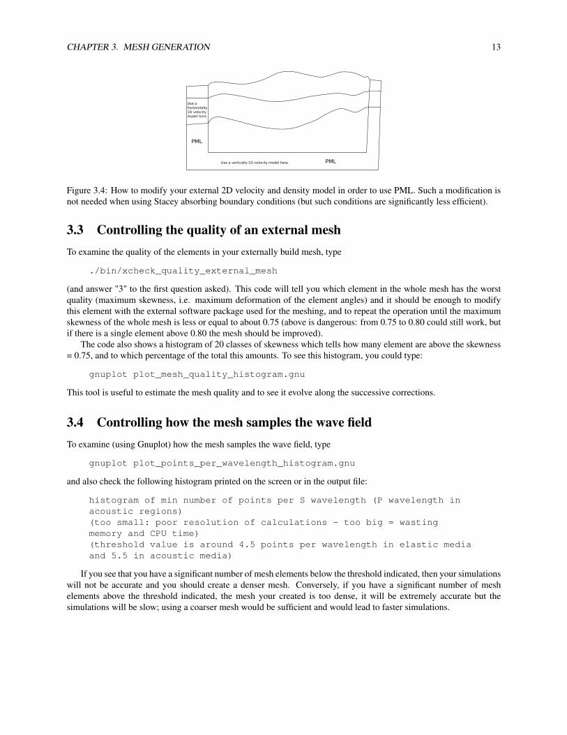
If you use PML and an external velocity and density model (e.g., setting flag “READ_EXTERNAL_SEP_FILE”to .true.), you should be careful because mathematically a PML cannot handle heterogeneities along the normalto the PML edge inside the PML layer. This comes from the fact that the damping profile that is defined assumes aconstant velocity and density model along the normal direction. Thus, you need to modify your velocity and densitymodel in order for it to be 1D inside the PML, as shown in Figure 3.4. This applies to the bottom layer as well; thereyou should make sure that your model is 1D and thus constant along the vertical direction. To summarize, only use a2D velocity and density model inside the physical region, and in all the PML layers extend it by continuity from itsvalues along the inner PML edge.
CHAPTER 3. MESH GENERATION 13
Use ahorizontally1D velocitymodel here
PML
PML
Use a vertically-1D velocity model here
Figure 3.4: How to modify your external 2D velocity and density model in order to use PML. Such a modification isnot needed when using Stacey absorbing boundary conditions (but such conditions are significantly less efficient).
3.3 Controlling the quality of an external meshTo examine the quality of the elements in your externally build mesh, type
./bin/xcheck_quality_external_mesh
(and answer "3" to the first question asked). This code will tell you which element in the whole mesh has the worstquality (maximum skewness, i.e. maximum deformation of the element angles) and it should be enough to modifythis element with the external software package used for the meshing, and to repeat the operation until the maximumskewness of the whole mesh is less or equal to about 0.75 (above is dangerous: from 0.75 to 0.80 could still work, butif there is a single element above 0.80 the mesh should be improved).
The code also shows a histogram of 20 classes of skewness which tells how many element are above the skewness= 0.75, and to which percentage of the total this amounts. To see this histogram, you could type:
gnuplot plot_mesh_quality_histogram.gnu
This tool is useful to estimate the mesh quality and to see it evolve along the successive corrections.
3.4 Controlling how the mesh samples the wave fieldTo examine (using Gnuplot) how the mesh samples the wave field, type
gnuplot plot_points_per_wavelength_histogram.gnu
and also check the following histogram printed on the screen or in the output file:
histogram of min number of points per S wavelength (P wavelength inacoustic regions)(too small: poor resolution of calculations - too big = wastingmemory and CPU time)(threshold value is around 4.5 points per wavelength in elastic mediaand 5.5 in acoustic media)
If you see that you have a significant number of mesh elements below the threshold indicated, then your simulationswill not be accurate and you should create a denser mesh. Conversely, if you have a significant number of meshelements above the threshold indicated, the mesh your created is too dense, it will be extremely accurate but thesimulations will be slow; using a coarser mesh would be sufficient and would lead to faster simulations.
Chapter 4
Running the Solver xspecfem2D
To run the solver, type:
./bin/xspecfem2D
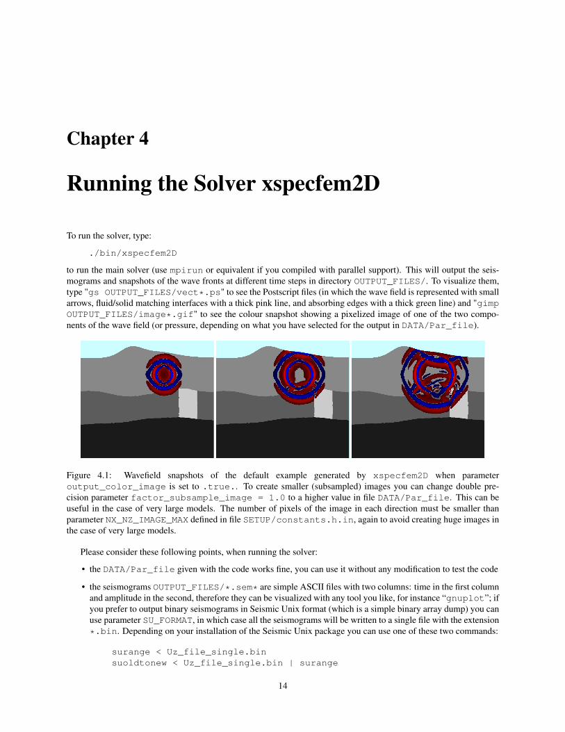
to run the main solver (use mpirun or equivalent if you compiled with parallel support). This will output the seis-mograms and snapshots of the wave fronts at different time steps in directory OUTPUT_FILES/. To visualize them,type "gs OUTPUT_FILES/vect*.ps" to see the Postscript files (in which the wave field is represented with smallarrows, fluid/solid matching interfaces with a thick pink line, and absorbing edges with a thick green line) and "gimpOUTPUT_FILES/image*.gif" to see the colour snapshot showing a pixelized image of one of the two compo-nents of the wave field (or pressure, depending on what you have selected for the output in DATA/Par_file).
Figure 4.1: Wavefield snapshots of the default example generated by xspecfem2D when parameteroutput_color_image is set to .true.. To create smaller (subsampled) images you can change double pre-cision parameter factor_subsample_image = 1.0 to a higher value in file DATA/Par_file. This can beuseful in the case of very large models. The number of pixels of the image in each direction must be smaller thanparameter NX_NZ_IMAGE_MAX defined in file SETUP/constants.h.in, again to avoid creating huge images inthe case of very large models.
Please consider these following points, when running the solver:
• the DATA/Par_file given with the code works fine, you can use it without any modification to test the code
• the seismograms OUTPUT_FILES/*.sem* are simple ASCII files with two columns: time in the first columnand amplitude in the second, therefore they can be visualized with any tool you like, for instance “gnuplot”; ifyou prefer to output binary seismograms in Seismic Unix format (which is a simple binary array dump) you canuse parameter SU_FORMAT, in which case all the seismograms will be written to a single file with the extension*.bin. Depending on your installation of the Seismic Unix package you can use one of these two commands:
surange < Uz_file_single.binsuoldtonew < Uz_file_single.bin | surange
14
CHAPTER 4. RUNNING THE SOLVER XSPECFEM2D 15
to see the header info. Replace surange with suxwigb to see wiggle plots for the seismograms.
• if you set flag assign_external_model to .true. in DATA/Par_file, the velocity and density modelthat is given at the end of DATA/Par_file is then ignored and overwritten by the external velocity and densitymodel that you define yourself in define_external_model.f90
• when compiling with Intel ifort, use “-assume byterecl” option to create binary PNM images displayingthe wave field
• there are a few useful scripts and Fortran routines in directory UTILS/.
• you can find a Fortran code to compute the analytical solution for simple media that we use as a reference inbenchmarks in many of our articles at (http://www.spice-rtn.org/library/software/EX2DDIR).That code is described in: Berg et al. [1994]
The SOURCE file located in the DATA/ directory should be edited in the following way:
source_surf Set this flag to .true. to force the source to be located at the surface of the model, otherwise thesol be placed inside the medium
xs source location x in meters
zs source location z in meters
source_type Set this value equal to 1 for elastic forces or acoustic pressure, set this to 2 for moment tensorsources. For a plane wave including converted and reflected waves at the free surface, P wave = 1, S wave = 2,Rayleigh wave = 3; for a plane wave without converted nor reflected waves at the free surface, i.e. the incidentwave only, P wave = 4, S wave = 5. (incident plane waves are turned on by parameter initialfield inDATA/Par_file).
time_function_type Choose a source-time function: set this value to 1 to use a Ricker, 2 the first derivative, 3a Gaussian, 4 a Dirac or 5 a Heaviside source-time function.
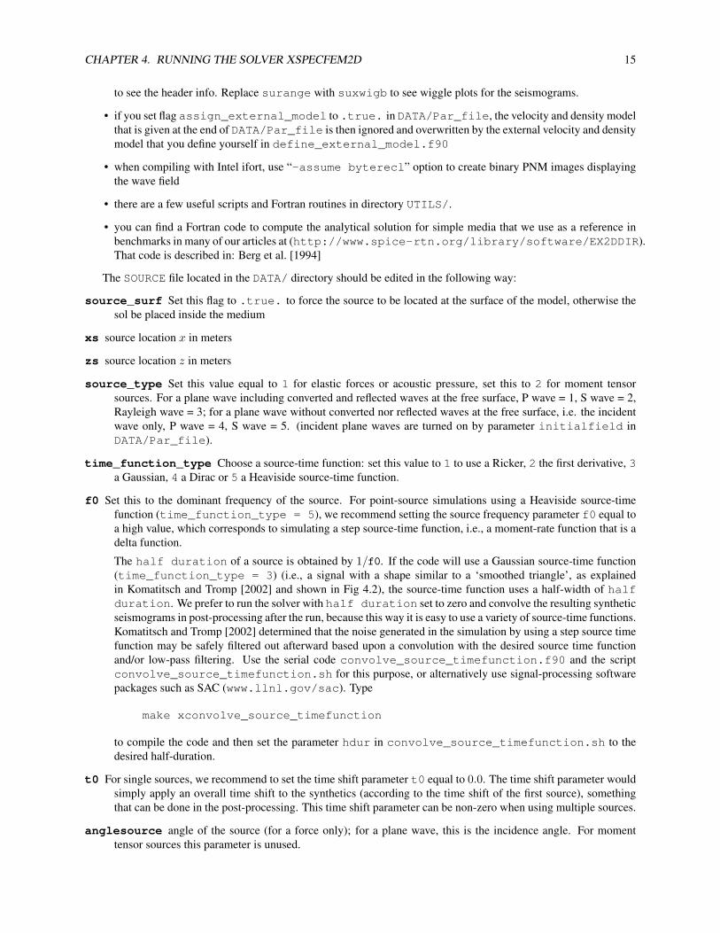
f0 Set this to the dominant frequency of the source. For point-source simulations using a Heaviside source-timefunction (time_function_type = 5), we recommend setting the source frequency parameter f0 equal toa high value, which corresponds to simulating a step source-time function, i.e., a moment-rate function that is adelta function.
The half duration of a source is obtained by 1/f0. If the code will use a Gaussian source-time function(time_function_type = 3) (i.e., a signal with a shape similar to a ‘smoothed triangle’, as explainedin Komatitsch and Tromp [2002] and shown in Fig 4.2), the source-time function uses a half-width of halfduration. We prefer to run the solver with half duration set to zero and convolve the resulting syntheticseismograms in post-processing after the run, because this way it is easy to use a variety of source-time functions.Komatitsch and Tromp [2002] determined that the noise generated in the simulation by using a step source timefunction may be safely filtered out afterward based upon a convolution with the desired source time functionand/or low-pass filtering. Use the serial code convolve_source_timefunction.f90 and the scriptconvolve_source_timefunction.sh for this purpose, or alternatively use signal-processing softwarepackages such as SAC (www.llnl.gov/sac). Type
make xconvolve_source_timefunction
to compile the code and then set the parameter hdur in convolve_source_timefunction.sh to thedesired half-duration.
t0 For single sources, we recommend to set the time shift parameter t0 equal to 0.0. The time shift parameter wouldsimply apply an overall time shift to the synthetics (according to the time shift of the first source), somethingthat can be done in the post-processing. This time shift parameter can be non-zero when using multiple sources.
anglesource angle of the source (for a force only); for a plane wave, this is the incidence angle. For momenttensor sources this parameter is unused.
CHAPTER 4. RUNNING THE SOLVER XSPECFEM2D 16
half duration
source decay rate
half duration
-
-
tCMT
Figure 4.2: Comparison of the shape of a triangle and the Gaussian function actually used.
Mxx,Mzz,Mxz Moment tensor components (valid only for moment tensor sources, source_type = 2). Notethat the units for the components of a moment tensor source are different in SPECFEM2D and in SPECFEM3D:
SPECFEM3D: in SPECFEM3D the moment tensor components are in dyne*cm
SPECFEM2D: in SPECFEM2D the moment tensor components are in N*m
To go from strike / dip / slip to CMTSOLUTION moment-tensor format using the classical formulas (of e.g.Aki and Richards [1980] you can use these two small C programs from SPECFEM3D_GLOBE:
./utils/strike_dip_rake_to_CMTSOLUTION.c
./utils/CMTSOLUTION_to_AkiRichards.c
but then it is another story to make a good 2D approximation of that, because in plain-strain P-SV what you getis the equivalent of a line source in the third direction (orthogonal to the plane) rather than a 3D point sourceFor more details on this see e.g. Section 7.3 "Two-dimensional point sources" of the book of Pilant [1979]. Thatbook being hard to find, we scanned the related pages in filediscussion_of_2D_sources_and_approximations_from_Pilant_1979.pdf in the same di-rectory as this users manual. Another very useful reference addressing that is Helmberger and Vidale [1988]and its recent extension (Global synthetic seismograms using a 2D finite-difference method, Dunzhu Li, DonHelmberger, Robert W. Clayton and Daoyuan Sun, submitted to Geophys. J. Int, 2014).
factor amplification factor
Note, the zero time of the simulation corresponds to the center of the triangle/Gaussian, or the centroid time ofthe earthquake. The start time of the simulation is t = −1.2 ∗ half duration + t0 (the factor 1.2 is to make surethe moment rate function is very close to zero when starting the simulation; Heaviside functions use a factor 2.0), thehalf duration is obtained by 1/f0. If you prefer, you can fix this start time by setting the parameter USER_T0 in theconstants.h file to a positive, non-zero value. The simulation in that case would start at a starting time equal to-USER_T0.
Coupled SimulationsThe code supports acoustic/elastic, acoustic/poroelastic, elastic/poroelastic, and acoustic, elastic/poroelastic simula-tions. Elastic/poroelastic coupling supports anisotropy, but not attenuation for the elastic material.
CHAPTER 4. RUNNING THE SOLVER XSPECFEM2D 17
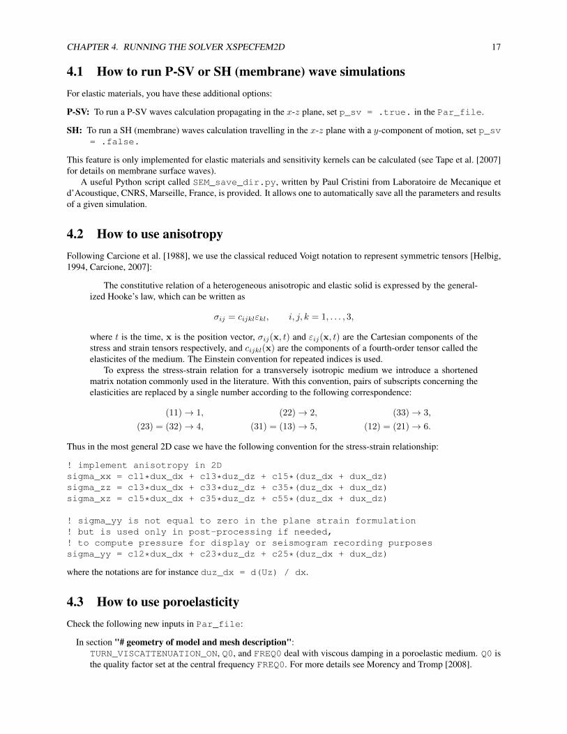
4.1 How to run P-SV or SH (membrane) wave simulationsFor elastic materials, you have these additional options:
P-SV: To run a P-SV waves calculation propagating in the x-z plane, set p_sv = .true. in the Par_file.
SH: To run a SH (membrane) waves calculation travelling in the x-z plane with a y-component of motion, set p_sv= .false.
This feature is only implemented for elastic materials and sensitivity kernels can be calculated (see Tape et al. [2007]for details on membrane surface waves).
A useful Python script called SEM_save_dir.py, written by Paul Cristini from Laboratoire de Mecanique etd’Acoustique, CNRS, Marseille, France, is provided. It allows one to automatically save all the parameters and resultsof a given simulation.
4.2 How to use anisotropyFollowing Carcione et al. [1988], we use the classical reduced Voigt notation to represent symmetric tensors [Helbig,1994, Carcione, 2007]:
The constitutive relation of a heterogeneous anisotropic and elastic solid is expressed by the general-ized Hooke’s law, which can be written as
σij = cijklεkl, i, j, k = 1, . . . , 3,
where t is the time, x is the position vector, σij(x, t) and εij(x, t) are the Cartesian components of thestress and strain tensors respectively, and cijkl(x) are the components of a fourth-order tensor called theelasticites of the medium. The Einstein convention for repeated indices is used.
To express the stress-strain relation for a transversely isotropic medium we introduce a shortenedmatrix notation commonly used in the literature. With this convention, pairs of subscripts concerning theelasticities are replaced by a single number according to the following correspondence:
(11)→ 1, (22)→ 2, (33)→ 3,
(23) = (32)→ 4, (31) = (13)→ 5, (12) = (21)→ 6.
Thus in the most general 2D case we have the following convention for the stress-strain relationship:
! implement anisotropy in 2Dsigma_xx = c11*dux_dx + c13*duz_dz + c15*(duz_dx + dux_dz)sigma_zz = c13*dux_dx + c33*duz_dz + c35*(duz_dx + dux_dz)sigma_xz = c15*dux_dx + c35*duz_dz + c55*(duz_dx + dux_dz)
! sigma_yy is not equal to zero in the plane strain formulation! but is used only in post-processing if needed,! to compute pressure for display or seismogram recording purposessigma_yy = c12*dux_dx + c23*duz_dz + c25*(duz_dx + dux_dz)
where the notations are for instance duz_dx = d(Uz) / dx.
4.3 How to use poroelasticityCheck the following new inputs in Par_file:
In section "# geometry of model and mesh description":TURN_VISCATTENUATION_ON, Q0, and FREQ0 deal with viscous damping in a poroelastic medium. Q0 isthe quality factor set at the central frequency FREQ0. For more details see Morency and Tromp [2008].
CHAPTER 4. RUNNING THE SOLVER XSPECFEM2D 18
In section "# time step parameters":SIMULATION_TYPE defines the type of simulation
(1) forward simulation
(2) UNUSED (purposely, for compatibility with the numbering convention used in our 3D codes)
(3) adjoint method and kernels calculation
In section "# source parameters":The code now support multiple sources. NSOURCE is the number of sources. Parameters of the sources aredisplayed in the file SOURCE, which must be in the directory DATA/. The components of a moment tensorsource must be given in N.m, not in dyne.cm as in the DATA/CMTSOLUTION source file of the 3D version ofthe code.
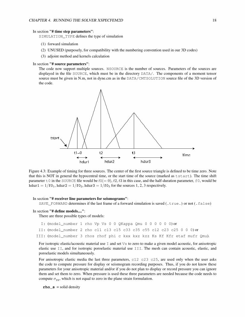
Figure 4.3: Example of timing for three sources. The center of the first source triangle is defined to be time zero. Notethat this is NOT in general the hypocentral time, or the start time of the source (marked as tstart). The time shiftparameter t0 in the SOURCE file would be t1(= 0), t2, t3 in this case, and the half-duration parameter, f0, would behdur1 = 1/f01, hdur2 = 1/f02, hdur3 = 1/f03 for the sources 1, 2, 3 respectively.
In section "# receiver line parameters for seismograms":SAVE_FORWARD determines if the last frame of a forward simulation is saved (.true.) or not (.false)
In section "# define models....":There are three possible types of models:
I: (model_number 1 rho Vp Vs 0 0 QKappa Qmu 0 0 0 0 0 0) or
II: (model_number 2 rho c11 c13 c15 c33 c35 c55 c12 c23 c25 0 0 0) or
III: (model_number 3 rhos rhof phi c kxx kxz kzz Ks Kf Kfr etaf mufr Qmu).
For isotropic elastic/acoustic material use I and set Vs to zero to make a given model acoustic, for anisotropicelastic use II, and for isotropic poroelastic material use III. The mesh can contain acoustic, elastic, andporoelastic models simultaneously.
For anisotropic elastic media the last three parameters, c12 c23 c25, are used only when the user asksthe code to compute pressure for display or seismogram recording purposes. Thus, if you do not know theseparameters for your anisotropic material and/or if you do not plan to display or record pressure you can ignorethem and set them to zero. When pressure is used these three parameters are needed because the code needs tocompute σyy , which is not equal to zero in the plane strain formulation.
rho_s = solid density
CHAPTER 4. RUNNING THE SOLVER XSPECFEM2D 19
rho_f = fluid density
phi = porosity
tort = tortuosity
permxx = xx component of permeability tensor
permxz = xz,zx components of permeability tensor
permzz = zz component of permeability tensor
kappa_s = solid bulk modulus
kappa_f = fluid bulk modulus
kappa_fr = frame bulk modulus
eta_f = fluid viscosity
mu_fr = frame shear modulus
Qmu = shear quality factor
Note: for the poroelastic case, mu_s is irrelevant. For details on the poroelastic theory see Morency and Tromp[2008].
get_poroelastic_velocities.f90 allows to compute cpI, cpII, and cs function of the source dominantfrequency. Notice that for this calculation we use permxx and the dominant frequency of the first source, f0(1).Caution if you use several sources with different frequencies and if you consider anistropic permeability.
4.4 How to set plane waves as initial conditionsTo simulate propagation of incoming plane waves in the simulation domain, initial conditions based on analyticalformulae of plane waves in homogeneous model need to be set. No additional body or boundary forces are required.To set up this scenario:
Par_file:
• switch on initialfield = .true.
• at this point setting add_bielak_condition does not seem to help with absorbing boundaries, there-fore, it should be turned off.
SOURCE:
• zs has to be the same as the height of the simulation domain defined in interfacesfile.
• xs is the x-coordinate of the intersection of the initial plane wave front with the free surface.
• source_type = 1 for a plane P wave, 2 for a plane SV wave, 3 for a Rayleigh wave.
• angleforce can be negative to indicate a plane wave incident from the right (instead of the left)
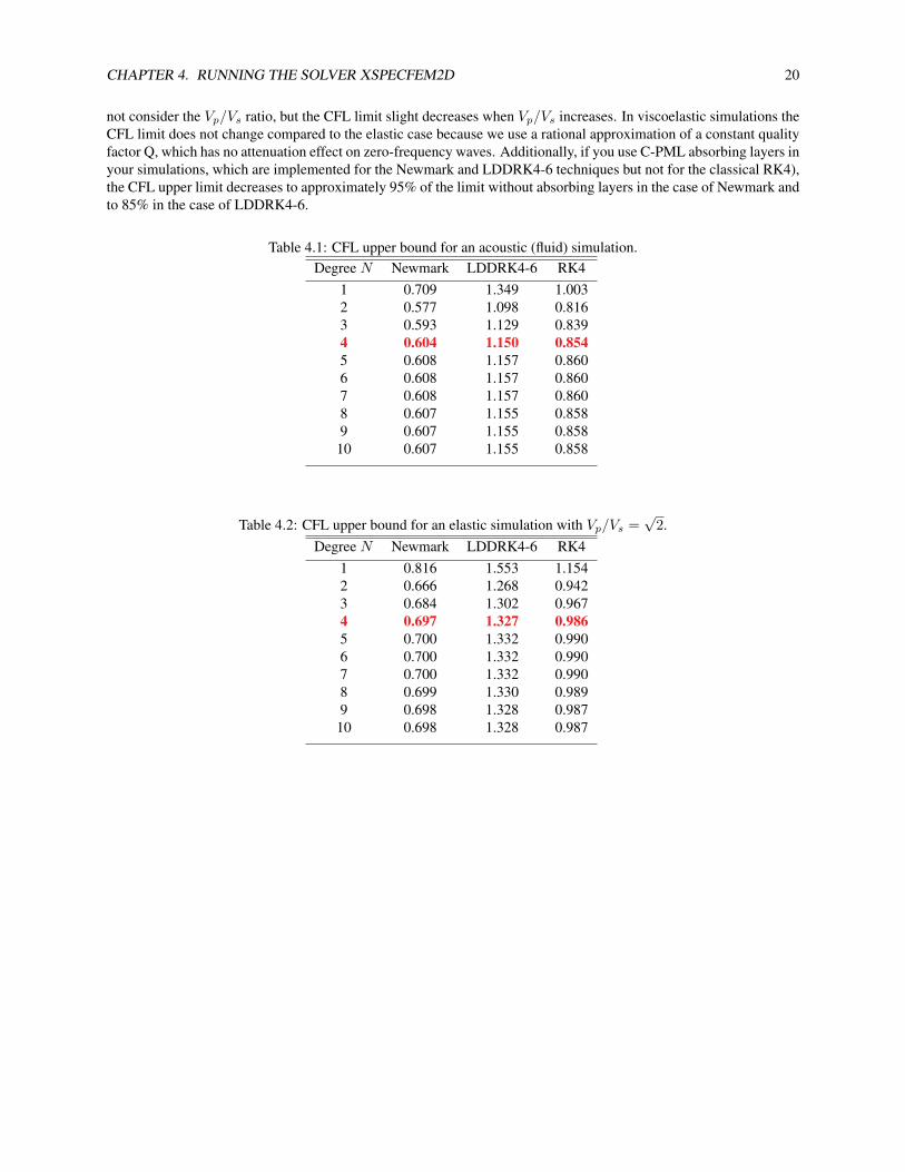
4.5 How to choose the time stepThree different explicit conditionally-stable time schemes can be used for elastic, acoustic (fluid) or coupled elas-tic/acoustic media: the Newmark method, the low-dissipation and low-dispersion fourth-order six-stage Runge-Kuttamethod (LDDRK4-6) presented in Berland et al. [2006], and the classical fourth-order four-stage Runge-Kutta (RK4)method. Currently the last two methods are not implemented for poroelastic media. According to De Basabe and Sen[2010] and Berland et al. [2006], with different degreesN = NGLLX−1 of the GLL basis functions the CFL boundsare given in the following tables. Note that by default the SPECFEM solver usesNGLLX = 5 and thus a degreeN =4, which is thus the value you should use in most cases in the following tables. You can directly compare these valueswith the value given in sentence ‘Max stability for P wave velocity’ in file output_solver.txt to see whether youset the correct ∆t in Par_file or not. For elastic simulation, the CFL value given in output_solver.txt does
CHAPTER 4. RUNNING THE SOLVER XSPECFEM2D 20
not consider the Vp/Vs ratio, but the CFL limit slight decreases when Vp/Vs increases. In viscoelastic simulations theCFL limit does not change compared to the elastic case because we use a rational approximation of a constant qualityfactor Q, which has no attenuation effect on zero-frequency waves. Additionally, if you use C-PML absorbing layers inyour simulations, which are implemented for the Newmark and LDDRK4-6 techniques but not for the classical RK4),the CFL upper limit decreases to approximately 95% of the limit without absorbing layers in the case of Newmark andto 85% in the case of LDDRK4-6.
Table 4.1: CFL upper bound for an acoustic (fluid) simulation.Degree N Newmark LDDRK4-6 RK4
1 0.709 1.349 1.0032 0.577 1.098 0.8163 0.593 1.129 0.8394 0.604 1.150 0.8545 0.608 1.157 0.8606 0.608 1.157 0.8607 0.608 1.157 0.8608 0.607 1.155 0.8589 0.607 1.155 0.858
10 0.607 1.155 0.858
Table 4.2: CFL upper bound for an elastic simulation with Vp/Vs =√
2.Degree N Newmark LDDRK4-6 RK4
1 0.816 1.553 1.1542 0.666 1.268 0.9423 0.684 1.302 0.9674 0.697 1.327 0.9865 0.700 1.332 0.9906 0.700 1.332 0.9907 0.700 1.332 0.9908 0.699 1.330 0.9899 0.698 1.328 0.987
10 0.698 1.328 0.987
Chapter 5
Adjoint Simulations
5.1 How to obtain Finite Sensitivity Kernels1. Run a forward simulation:
• SIMULATION_TYPE = 1
• SAVE_FORWARD = .true.
• seismotype = 1 (we need to save the displacement fields to later on derive the adjoint source. Note: ifthe user forgets it, the program corrects it when reading the proper SIMULATION_TYPE and SAVE_FORWARDcombination and a warning message appears in the output file)
Important output files (for example, for the elastic case, P-SV waves):
• absorb_elastic_bottom*****.bin
• absorb_elastic_left*****.bin
• absorb_elastic_right*****.bin
• absorb_elastic_top*****.bin
• lastframe_elastic*****.bin
• S****.AA.BXX.semd
• S****.AA.BXZ.semd
2. Define the adjoint source:
• Use adj_seismogram.f90
• Edit to update NSTEP, nrec, t0, deltat, and the position of the cut to pick any given phase if needed(tstart,tend), add the right number of stations, and put one component of the source to zero if needed.
• The output files of adj_seismogram.f90 are S****.AA.BXX.adj and S****.AA.BXZ.adj,for P-SV waves (and S****.AA.BXY.adj, for SH (membrane) waves). Note that you will need thesethree files (S****.AA.BXX.adj, S****.AA.BXY.adj and S****.AA.BXZ.adj) to be present inthe SEM/ directory together with the absorb_elastic_****.bin and lastframe_elastic.binfiles to be read when running the adjoint simulation.
3. Run the adjoint simulation:
• Make sure that the adjoint source files absorbing boundaries and last frame files are in the OUTPUT_FILES/directory.
• SIMULATION_TYPE = 3
• SAVE_FORWARD = .false.
21
CHAPTER 5. ADJOINT SIMULATIONS 22
Output files (for example for the elastic case):
• snapshot_rho_kappa_mu*****
• snapshot_rhop_alpha_beta*****
which are the primary moduli kernels and the phase velocities kernels respectively, in ascii format and at thelocal level, that is as “kernels(i,j,ispec)”.
5.2 Remarks about adjoint runs and solving inverse problemsSPECFEM2D can produce the gradient of the misfit function for a tomographic inversion, but options for using thegradient within an iterative inversion are left to the user (e.g., conjugate-gradient, steepest descent). The plan is toinclude some examples in the future.
The algorithm is simple:
1. calculate the forward wave field s(x, t)
2. calculate the adjoint wave field s†(x, t)
3. calculate their interaction s(x, t) · s†(x, T − t) (these symbolic, temporal and spatial derivatives should beincluded)
4. integrate the interactions, which is summation in the code.
That is all. Step 3 has some tricks in implementation, but which can be skipped by regular users.If you look into SPECFEM2D, besides “rhop_ac_kl” and “rho_ac_kl”, there are more variables such as
“kappa_ac_kl” and “rho_el_kl” etc. “rho” denotes density ρ (“kappa” for bulk modulus κ etc.), “ac”denotes acoustic (“el” for elastic), “kl” means kernel (and you may find “k” as well, which is the interaction at eachtime step, i.e., before doing time integration).
5.3 CautionPlease note that:
• at the moment, adjoint simulations do not support anisotropy, attenuation, and viscous damping.
• you will need S****.AA.BXX.adj, S****.AA.BXY.adj and S****.AA.BXZ.adj to be present indirectory SEM/ even if you are just running an acoustic or poroelastic adjoint simulation.
– S****.AA.BXX.adj is the only relevant component for an acoustic case.
– S****.AA.BXX.adj and S****.AA.BXZ.adj are the only relevant components for a poroelasticcase.
Chapter 6
Oil and gas industry simulations
The SPECFEM2D package provides compatibility with industrial (oil and gas industry) types of simulations. Thesefeatures include importing Seismic Unix (SU) format wavespeed models into SPECFEM2D, output of seismogramsin SU format with a few key parameters defined in the trace headers and reading adjoint sources in SU format etc.There is one example given in EXAMPLES/INDUSTRIAL_FORMAT, which you can follow.
We also changed the relationship between adjoint potential and adjoint displacement in fluid region (the relation-ship between forward potential and forward displacement remains the same as previously defined). The new definitionis critical when there are adjoint sources (in other words, receivers) in the acoustic domain, and is the direct conse-quence of the optimization problem.
s ≡ 1
ρ∇φ
p ≡ −κ (∇ · s) = −∂2t φ
∂2t s† ≡ −1
ρ∇φ†
p† ≡ −κ(∇ · s†
)= φ†
23
Acknowledgments
The Gauss-Lobatto-Legendre subroutines in gll_library.f90 are based in part on software libraries from theMassachusetts Institute of Technology, Department of Mechanical Engineering (Cambridge, Massachusetts, USA).The non-structured global numbering software was provided by Paul F. Fischer (Brown University, Providence, RhodeIsland, USA, now at Argonne National Laboratory, USA).
Please e-mail your feedback, bug reports, questions, comments, and suggestions to the CIG Computational Seis-mology Mailing List ([email protected]).
24

Copyright
Main historical authors: Dimitri Komatitsch and Jeroen Tromp
Princeton University, USA, and CNRS / University of Marseille, France
© Princeton University and CNRS / University of Marseille, July 2012
25

Bibliography
C. A. Acosta Minolia and D. A. Kopriva. Discontinuous Galerkin spectral element approximations on moving meshes.J. Comput. Phys., 230(5):1876–1902, 2011. doi: 10.1016/j.jcp.2010.11.038.
M. Ainsworth and H. Wajid. Dispersive and dissipative behavior of the spectral element method. SIAM Journal onNumerical Analysis, 47(5):3910–3937, 2009. doi: 10.1137/080724976.
M. Ainsworth and H. Wajid. Optimally blended spectral-finite element scheme for wave propagation and nonstandardreduced integration. SIAM Journal on Numerical Analysis, 48(1):346–371, 2010. doi: 10.1137/090754017.
M. Ainsworth, P. Monk, and W. Muniz. Dispersive and dissipative properties of discontinuous Galerkin finite elementmethods for the second-order wave equation. Journal of Scientific Computing, 27(1):5–40, 2006. doi: 10.1007/s10915-005-9044-x.
K. Aki and P. G. Richards. Quantitative seismology, theory and methods. W. H. Freeman, San Francisco, USA, 1980.
D. N. Arnold. An interior penalty finite element method with discontinuous elements. SIAM Journal on NumericalAnalysis, 19(4):742–760, 1982. doi: 10.1137/0719052.
M. Benjemaa, N. Glinsky-Olivier, V. M. Cruz-Atienza, J. Virieux, and S. Piperno. Dynamic non-planar crack ruptureby a finite volume method. Geophys. J. Int., 171(1):271–285, 2007. doi: 10.1111/j.1365-246X.2006.03500.x.
M. Benjemaa, N. Glinsky-Olivier, V. M. Cruz-Atienza, and J. Virieux. 3D dynamic rupture simulation by a finitevolume method. Geophys. J. Int., 178(1):541–560, 2009. doi: 10.1111/j.1365-246X.2009.04088.x.
P. Berg, F. If, P. Nielsen, and O. Skovegaard. Analytic reference solutions. In K. Helbig, editor, Modeling the Earth foroil exploration, Final report of the CEC’s GEOSCIENCE I Program 1990-1993, pages 421–427. Pergamon Press,Oxford, United Kingdom, 1994.
J. Berland, C. Bogey, and C. Bailly. Low-dissipation and low-dispersion fourth-order Runge-Kutta algorithm. Com-puters and Fluids, 35:1459–1463, 2006.
M. Bernacki, S. Lanteri, and S. Piperno. Time-domain parallel simulation of heterogeneous wave propagation onunstructured grids using explicit, nondiffusive, discontinuous Galerkin methods. J. Comput. Acoust., 14(1):57–81,2006.
C. Bernardi, Y. Maday, and A. T. Patera. A new nonconforming approach to domain decomposition: the Mortarelement method. In H. Brezis and J. L. Lions, editors, Nonlinear partial differential equations and their applications,Séminaires du Collège de France, pages 13–51, Paris, 1994. Pitman.
F. Bourdel, P.-A. Mazet, and P. Helluy. Resolution of the non-stationary or harmonic Maxwell equations by a discon-tinuous finite element method: Application to an E.M.I. (electromagnetic impulse) case. In Proceedings of the 10thinternational conference on computing methods in applied sciences and engineering, pages 405–422, Commack,NY, USA, 1991. Nova Science Publishers, Inc.
J. M. Carcione. Wave fields in real media: Theory and numerical simulation of wave propagation in anisotropic,anelastic, porous and electromagnetic media. Elsevier Science, Amsterdam, The Netherlands, second edition,2007.
26
BIBLIOGRAPHY 27
J. M. Carcione, D. Kosloff, and R. Kosloff. Wave propagation simulation in an elastic anisotropic (transverselyisotropic) solid. Q. J. Mech. Appl. Math., 41(3):319–345, 1988.
L. Carrington, D. Komatitsch, M. Laurenzano, M. Tikir, D. Michéa, N. Le Goff, A. Snavely, and J. Tromp. High-frequency simulations of global seismic wave propagation using SPECFEM3D_GLOBE on 62 thousand processorcores. In Proceedings of the SC’08 ACM/IEEE conference on Supercomputing, pages 60:1–60:11, Austin, Texas,USA, Nov. 2008. IEEE Press. doi: 10.1145/1413370.1413432. Article #60, Gordon Bell Prize finalist article.
F. Casadei and E. Gabellini. Implementation of a 3D coupled Spectral Element solver for wave propagation andsoil-structure interaction simulations. Technical report, European Commission Joint Research Center ReportEUR17730EN, Ispra, Italy, 1997.
E. Chaljub. Modélisation numérique de la propagation d’ondes sismiques en géométrie sphérique : application à lasismologie globale (Numerical modeling of the propagation of seismic waves in spherical geometry: application toglobal seismology). PhD thesis, Université Paris VII Denis Diderot, Paris, France, 2000.
E. Chaljub, Y. Capdeville, and J. P. Vilotte. Solving elastodynamics in a fluid-solid heterogeneous sphere: a parallelspectral-element approximation on non-conforming grids. J. Comput. Phys., 187(2):457–491, 2003.
E. Chaljub, D. Komatitsch, J. P. Vilotte, Y. Capdeville, B. Valette, and G. Festa. Spectral element analysis in seismol-ogy. In R.-S. Wu and V. Maupin, editors, Advances in wave propagation in heterogeneous media, volume 48 ofAdvances in Geophysics, pages 365–419. Elsevier - Academic Press, London, UK, 2007.
B. Cockburn, G. E. Karniadakis, and C.-W. Shu. Discontinuous Galerkin Methods: Theory, Computation and Appli-cations. Springer, Heidelberg, Germany, 2000.
G. Cohen. Higher-order numerical methods for transient wave equations. Springer-Verlag, Berlin, Germany, 2002.
G. Cohen, P. Joly, and N. Tordjman. Construction and analysis of higher-order finite elements with mass lumping forthe wave equation. In R. Kleinman, editor, Proceedings of the second international conference on mathematicaland numerical aspects of wave propagation, pages 152–160. SIAM, Philadelphia, Pennsylvania, USA, 1993.
J. D. De Basabe and M. K. Sen. Grid dispersion and stability criteria of some common finite-element methods foracoustic and elastic wave equations. Geophysics, 72(6):T81–T95, 2007. doi: 10.1190/1.2785046.
J. D. De Basabe and M. K. Sen. Stability of the high-order finite elements for acoustic or elastic wave propagationwith high-order time stepping. Geophys. J. Int., 181(1):577–590, 2010. doi: 10.1111/j.1365-246X.2010.04536.x.
J. D. De Basabe, M. K. Sen, and M. F. Wheeler. The interior penalty discontinuous Galerkin method for elastic wavepropagation: grid dispersion. Geophys. J. Int., 175(1):83–93, 2008. doi: 10.1111/j.1365-246X.2008.03915.x.
J. de la Puente, J. P. Ampuero, and M. Käser. Dynamic rupture modeling on unstructured meshes using a discontinuousGalerkin method. J. Geophys. Res., 114:B10302, 2009. doi: 10.1029/2008JB006271.
M. O. Deville, P. F. Fischer, and E. H. Mund. High-Order Methods for Incompressible Fluid Flow. CambridgeUniversity Press, Cambridge, United Kingdom, 2002.
M. Dumbser and M. Käser. An arbitrary high-order discontinuous Galerkin method for elastic waves on un-structured meshes-II. The three-dimensional isotropic case. Geophys. J. Int., 167(1):319–336, 2006. doi:10.1111/j.1365-246X.2006.03120.x.
V. Étienne, E. Chaljub, J. Virieux, and N. Glinsky. An hp-adaptive discontinuous Galerkin finite-element method for3-D elastic wave modelling. Geophys. J. Int., 183(2):941–962, 2010. doi: 10.1111/j.1365-246X.2010.04764.x.
E. Faccioli, F. Maggio, R. Paolucci, and A. Quarteroni. 2D and 3D elastic wave propagation by a pseudo-spectraldomain decomposition method. J. Seismol., 1:237–251, 1997.
R. S. Falk and G. R. Richter. Explicit finite element methods for symmetric hyperbolic equations. SIAM Journal onNumerical Analysis, 36(3):935–952, 1999. doi: 10.1137/S0036142997329463.
BIBLIOGRAPHY 28
F. X. Giraldo, J. S. Hesthaven, and T. Warburton. Nodal high-order discontinuous Galerkin methods for the sphericalshallow water equations. J. Comput. Phys., 181(2):499–525, 2002. doi: 10.1006/jcph.2002.7139.
L. Godinho, P. A. Mendes, A. Tadeu, A. Cadena-Isaza, C. Smerzini, F. J. Sánchez-Sesma, R. Madec, and D. Ko-matitsch. Numerical simulation of ground rotations along 2D topographical profiles under the incidence of elasticplane waves. Bull. Seismol. Soc. Am., 99(2B):1147–1161, 2009. doi: 10.1785/0120080096.
W. Gropp, E. Lusk, and A. Skjellum. Using MPI, portable parallel programming with the Message-Passing Interface.MIT Press, Cambridge, USA, 1994.
M. J. Grote, A. Schneebeli, and D. Schötzau. Discontinuous Galerkin finite element method for the wave equation.SIAM Journal on Numerical Analysis, 44(6):2408–2431, 2006. doi: 10.1137/05063194X.
K. Helbig. Foundations of anisotropy for exploration seismics. In K. Helbig and S. Treitel, editors, Handbook ofGeophysical exploration, section I: Seismic exploration, volume 22. Pergamon, Oxford, England, 1994.
D. V. Helmberger and J. E. Vidale. Modeling strong motions produced by earthquakes with two-dimensional numericalcodes. Bull. Seismol. Soc. Am., 78(1):109–121, 1988.
F. Q. Hu, M. Y. Hussaini, and P. Rasetarinera. An analysis of the discontinuous Galerkin method for wave propagationproblems. J. Comput. Phys., 151(2):921–946, 1999. doi: 10.1006/jcph.1999.6227.
C. Johnson and J. Pitkäranta. An analysis of the discontinuous Galerkin method for a scalar hyperbolic equation.Math. Comp., 46:1–26, 1986. doi: 10.1090/S0025-5718-1986-0815828-4.
D. Komatitsch. Méthodes spectrales et éléments spectraux pour l’équation de l’élastodynamique 2D et 3D en milieuhétérogène (Spectral and spectral-element methods for the 2D and 3D elastodynamics equations in heterogeneousmedia). PhD thesis, Institut de Physique du Globe, Paris, France, May 1997. 187 pages.
D. Komatitsch. Fluid-solid coupling on a cluster of GPU graphics cards for seismic wave propagation. C. R. Acad.Sci., Ser. IIb Mec., 339:125–135, 2011. doi: 10.1016/j.crme.2010.11.007.
D. Komatitsch and R. Martin. An unsplit convolutional Perfectly Matched Layer improved at grazing incidence forthe seismic wave equation. Geophysics, 72(5):SM155–SM167, 2007. doi: 10.1190/1.2757586.
D. Komatitsch and J. Tromp. Introduction to the spectral-element method for 3-D seismic wave propagation. Geophys.J. Int., 139(3):806–822, 1999. doi: 10.1046/j.1365-246x.1999.00967.x.
D. Komatitsch and J. Tromp. Spectral-element simulations of global seismic wave propagation-I. Validation. Geophys.J. Int., 149(2):390–412, 2002. doi: 10.1046/j.1365-246X.2002.01653.x.
D. Komatitsch and J. P. Vilotte. The spectral-element method: an efficient tool to simulate the seismic response of 2Dand 3D geological structures. Bull. Seismol. Soc. Am., 88(2):368–392, 1998.
D. Komatitsch, R. Martin, J. Tromp, M. A. Taylor, and B. A. Wingate. Wave propagation in 2-D elastic mediausing a spectral element method with triangles and quadrangles. J. Comput. Acoust., 9(2):703–718, 2001. doi:10.1142/S0218396X01000796.
D. Komatitsch, S. Tsuboi, C. Ji, and J. Tromp. A 14.6 billion degrees of freedom, 5 teraflops, 2.5 terabyte earthquakesimulation on the Earth Simulator. In Proceedings of the SC’03 ACM/IEEE conference on Supercomputing, pages4–11, Phoenix, Arizona, USA, Nov. 2003. ACM. doi: 10.1145/1048935.1050155. Gordon Bell Prize winner article.
D. Komatitsch, Q. Liu, J. Tromp, P. Süss, C. Stidham, and J. H. Shaw. Simulations of ground motion in the LosAngeles basin based upon the spectral-element method. Bull. Seismol. Soc. Am., 94(1):187–206, 2004. doi: 10.1785/0120030077.
D. Komatitsch, J. Labarta, and D. Michéa. A simulation of seismic wave propagation at high resolution in the innercore of the Earth on 2166 processors of MareNostrum. Lecture Notes in Computer Science, 5336:364–377, 2008.
BIBLIOGRAPHY 29
D. Komatitsch, D. Michéa, and G. Erlebacher. Porting a high-order finite-element earthquake modeling application toNVIDIA graphics cards using CUDA. Journal of Parallel and Distributed Computing, 69(5):451–460, 2009. doi:10.1016/j.jpdc.2009.01.006.
D. Komatitsch, G. Erlebacher, D. Göddeke, and D. Michéa. High-order finite-element seismic wave propagationmodeling with MPI on a large GPU cluster. J. Comput. Phys., 229(20):7692–7714, 2010a. doi: 10.1016/j.jcp.2010.06.024.
D. Komatitsch, L. P. Vinnik, and S. Chevrot. SHdiff/SVdiff splitting in an isotropic Earth. J. Geophys. Res., 115(B7):B07312, 2010b. doi: 10.1029/2009JB006795.
D. A. Kopriva. Metric identities and the discontinuous spectral element method on curvilinear meshes. Journal ofScientific Computing, 26(3):301–327, 2006. doi: 10.1007/s10915-005-9070-8.
D. A. Kopriva, S. L. Woodruff, and M. Y. Hussaini. Computation of electromagnetic scattering with a non-conformingdiscontinuous spectral element method. Int. J. Numer. Meth. Eng., 53(1):105–122, 2002. doi: 10.1002/nme.394.
S. J. Lee, H. W. Chen, Q. Liu, D. Komatitsch, B. S. Huang, and J. Tromp. Three-dimensional simulations of seismicwave propagation in the Taipei basin with realistic topography based upon the spectral-element method. Bull.Seismol. Soc. Am., 98(1):253–264, 2008. doi: 10.1785/0120070033.
S. J. Lee, Y. C. Chan, D. Komatitsch, B. S. Huang, and J. Tromp. Effects of realistic surface topography on seismicground motion in the Yangminshan region of Taiwan based upon the spectral-element method and LiDAR DTM.Bull. Seismol. Soc. Am., 99(2A):681–693, 2009a. doi: 10.1785/0120080264.
S. J. Lee, D. Komatitsch, B. S. Huang, and J. Tromp. Effects of topography on seismic wave propagation: An examplefrom northern Taiwan. Bull. Seismol. Soc. Am., 99(1):314–325, 2009b. doi: 10.1785/0120080020.
A. Legay, H. W. Wang, and T. Belytschko. Strong and weak arbitrary discontinuities in spectral finite elements. Int. J.Numer. Meth. Eng., 64(8):991–1008, 2005. doi: 10.1002/nme.1388.
P. Lesaint and P. A. Raviart. On a finite element method for solving the neutron transport equation (Proc. Symposium,Mathematical Research Center). In U. of Wisconsin-Madison, editor, Mathematical aspects of finite elements inpartial differential equations, volume 33, pages 89–123, New York, USA, 1974. Academic Press.
Q. Liu and J. Tromp. Finite-frequency kernels based on adjoint methods. Bull. Seismol. Soc. Am., 96(6):2383–2397,2006. doi: 10.1785/0120060041.
Q. Liu, J. Polet, D. Komatitsch, and J. Tromp. Spectral-element moment tensor inversions for earthquakes in SouthernCalifornia. Bull. Seismol. Soc. Am., 94(5):1748–1761, 2004. doi: 10.1785/012004038.
Y. Maday and A. T. Patera. Spectral-element methods for the incompressible Navier-Stokes equations. In State of theart survey in computational mechanics, pages 71–143, 1989. A. K. Noor and J. T. Oden editors.
R. Martin and D. Komatitsch. An unsplit convolutional perfectly matched layer technique improved at grazing inci-dence for the viscoelastic wave equation. Geophys. J. Int., 179(1):333–344, 2009. doi: 10.1111/j.1365-246X.2009.04278.x.
R. Martin, D. Komatitsch, C. Blitz, and N. Le Goff. Simulation of seismic wave propagation in an asteroid based uponan unstructured MPI spectral-element method: blocking and non-blocking communication strategies. Lecture Notesin Computer Science, 5336:350–363, 2008a.
R. Martin, D. Komatitsch, and A. Ezziani. An unsplit convolutional perfectly matched layer improved at grazingincidence for seismic wave equation in poroelastic media. Geophysics, 73(4):T51–T61, 2008b. doi: 10.1190/1.2939484.
R. Martin, D. Komatitsch, and S. D. Gedney. A variational formulation of a stabilized unsplit convolutional perfectlymatched layer for the isotropic or anisotropic seismic wave equation. Comput. Model. Eng. Sci., 37(3):274–304,2008c.
BIBLIOGRAPHY 30
R. Martin, D. Komatitsch, S. D. Gedney, and E. Bruthiaux. A high-order time and space formulation of the unsplitperfectly matched layer for the seismic wave equation using Auxiliary Differential Equations (ADE-PML). Comput.Model. Eng. Sci., 56(1):17–42, 2010.
T. Melvin, A. Staniforth, and J. Thuburn. Dispersion analysis of the spectral-element method. Quarterly Journal ofthe Royal Meteorological Society, 138(668):1934–1947, 2012. doi: 10.1002/qj.1906.
E. D. Mercerat, J. P. Vilotte, and F. J. Sánchez-Sesma. Triangular spectral-element simulation of two-dimensionalelastic wave propagation using unstructured triangular grids. Geophys. J. Int., 166(2):679–698, 2006.
D. Michéa and D. Komatitsch. Accelerating a 3D finite-difference wave propagation code using GPU graphics cards.Geophys. J. Int., 182(1):389–402, 2010. doi: 10.1111/j.1365-246X.2010.04616.x.
P. Monk and G. R. Richter. A discontinuous Galerkin method for linear symmetric hyperbolic systems in inhomoge-neous media. Journal of Scientific Computing, 22-23(1-3):443–477, 2005. doi: 10.1007/s10915-004-4132-5.
C. Morency and J. Tromp. Spectral-element simulations of wave propagation in poroelastic media. Geophys. J. Int.,175:301–345, 2008.
C. Morency, Y. Luo, and J. Tromp. Finite-frequency kernels for wave propagation in porous media based upon adjointmethods. Geophys. J. Int., 179:1148–1168, 2009. doi: 10.1111/j.1365-246X.2009.04332.
S. P. Oliveira and G. Seriani. Effect of element distortion on the numerical dispersion of spectral-element methods.Communications in Computational Physics, 9(4):937–958, 2011.
P. S. Pacheco. Parallel programming with MPI. Morgan Kaufmann Press, San Francisco, USA, 1997.
A. T. Patera. A spectral element method for fluid dynamics: laminar flow in a channel expansion. J. Comput. Phys.,54:468–488, 1984.
F. Pellegrini and J. Roman. SCOTCH: A software package for static mapping by dual recursive bipartitioning ofprocess and architecture graphs. Lecture Notes in Computer Science, 1067:493–498, 1996.
D. Peter, D. Komatitsch, Y. Luo, R. Martin, N. Le Goff, E. Casarotti, P. Le Loher, F. Magnoni, Q. Liu, C. Blitz,T. Nissen-Meyer, P. Basini, and J. Tromp. Forward and adjoint simulations of seismic wave propagation on fullyunstructured hexahedral meshes. Geophys. J. Int., 186(2):721–739, 2011. doi: 10.1111/j.1365-246X.2011.05044.x.
W. L. Pilant. Elastic waves in the Earth, volume 11 of "Developments in Solid Earth Geophysics" Series. ElsevierScientific Publishing Company, Amsterdam, The Netherlands, 1979.
E. Priolo, J. M. Carcione, and G. Seriani. Numerical simulation of interface waves by high-order spectral modelingtechniques. J. Acoust. Soc. Am., 95(2):681–693, 1994.
W. H. Reed and T. R. Hill. Triangular mesh methods for the neutron transport equation. Technical Report LA-UR-73-479, Los Alamos Scientific Laboratory, Los Alamos, USA, 1973.
B. Rivière and M. F. Wheeler. Discontinuous finite element methods for acoustic and elastic wave problems. Contem-porary Mathematics, 329:271–282, 2003.
G. Seriani and S. P. Oliveira. Optimal blended spectral-element operators for acoustic wave modeling. Geophysics,72(5):SM95–SM106, 2007. doi: 10.1190/1.2750715.
G. Seriani and S. P. Oliveira. Dispersion analysis of spectral-element methods for elastic wave propagation. WaveMotion, 45:729–744, 2008. doi: 10.1016/j.wavemoti.2007.11.007.
G. Seriani and E. Priolo. A spectral element method for acoustic wave simulation in heterogeneous media. FiniteElements in Analysis and Design, 16:337–348, 1994.
G. Seriani, E. Priolo, and A. Pregarz. Modelling waves in anisotropic media by a spectral element method. InG. Cohen, editor, Proceedings of the third international conference on mathematical and numerical aspects of wavepropagation, pages 289–298. SIAM, Philadephia, PA, 1995.

BIBLIOGRAPHY 31
J. Tago, V. M. Cruz-Atienza, V. Étienne, J. Virieux, M. Benjemaa, and F. J. Sánchez-Sesma. 3D dy-namic rupture with anelastic wave propagation using an hp-adaptive Discontinuous Galerkin method. In Ab-stract S51A-1915 presented at 2010 AGU Fall Meeting, San Francisco, California, USA, December 2010.www.agu.org/meetings/fm10/waisfm10.html.
C. Tape, Q. Liu, and J. Tromp. Finite-frequency tomography using adjoint methods - Methodology and examples usingmembrane surface waves. Geophys. J. Int., 168(3):1105–1129, 2007. doi: 10.1111/j.1365-246X.2006.03191.x.
M. A. Taylor and B. A. Wingate. A generalized diagonal mass matrix spectral element method for non-quadrilateralelements. Appl. Num. Math., 33:259–265, 2000.
J. Tromp, D. Komatitsch, and Q. Liu. Spectral-element and adjoint methods in seismology. Communications inComputational Physics, 3(1):1–32, 2008.
S. Tsuboi, D. Komatitsch, C. Ji, and J. Tromp. Broadband modeling of the 2002 Denali fault earthquake on the EarthSimulator. Phys. Earth Planet. In., 139(3-4):305–313, 2003. doi: 10.1016/j.pepi.2003.09.012.
R. Vai, J. M. Castillo-Covarrubias, F. J. Sánchez-Sesma, D. Komatitsch, and J. P. Vilotte. Elastic wave propagationin an irregularly layered medium. Soil Dynamics and Earthquake Engineering, 18(1):11–18, 1999. doi: 10.1016/S0267-7261(98)00027-X.
K. van Wijk, D. Komatitsch, J. A. Scales, and J. Tromp. Analysis of strong scattering at the micro-scale. J. Acoust.Soc. Am., 115(3):1006–1011, 2004. doi: 10.1121/1.1647480.
L. C. Wilcox, G. Stadler, C. Burstedde, and O. Ghattas. A high-order discontinuous Galerkin method for wavepropagation through coupled elastic-acoustic media. J. Comput. Phys., 229(24):9373–9396, 2010. doi: 10.1016/j.jcp.2010.09.008.
B. A. Wingate and J. P. Boyd. Spectral element methods on triangles for geophysical fluid dynamics problems. InA. V. Ilin and L. R. Scott, editors, Proceedings of the Third International Conference on Spectral and High-orderMethods, pages 305–314, Houston, Texas, 1996. Houston J. Mathematics.
Appendix A
Troubleshooting
FAQ
Regarding the structure of some of the database filesQuestion: Can anyone tell me what the columns of the SPECFEM2D boundary condition files in SPECFEM2D/DATA/Mesh_canyon are?
SPECFEM2D/DATA/Mesh_canyon/canyon_absorbing_surface_fileSPECFEM2D/DATA/Mesh_canyon/canyon_free_surface_file
Answer: canyon_absorbing_surface_file refers to parameters related to the absorbing conditions: Thefirst number (180) is the number of absorbing elements (nelemabs in the code). Then the columns are:
column 1: the element number
column 2: the number of nodes of this element that form the absorbing surface
column 3: the first node
column 4: the second node
canyon_free_surface_file refers to the elements of the free surface (relevant for enforcing free surfacecondition for acoustic media): The first number (160) is the number of elements of the free surface. Then the columnsare (similar to the absorbing case):
column 1: the element number
column 2: the number of nodes of this element that form the absorbing surface
column 3: the first node
column 4: the second node
Concerning the free surface description file, nodes/edges pertaining to elastic elements are discarded when the fileis read (if for whatever reason it was simpler to include all the nodes/edges on one side of a studied area and that thereare among them some elements that are elastic elements, only the nodes/edges of acoustic elements are kept).
These files are opened and read in meshfem2D.F90 using subroutines read_abs_surface() and read_acoustic_surface(), which are in part_unstruct.F90
32
Appendix B
License
CeCILL FREE SOFTWARE LICENSE AGREEMENTAvailable online at http://www.cecill.info/licences/Licence_CeCILL_V2-en.htmlNoticeThis Agreement is a Free Software license agreement that is the result of discussions between its authors in order
to ensure compliance with the two main principles guiding its drafting:- firstly, compliance with the principles governing the distribution of Free Software: access to source code, broad
rights granted to users,- secondly, the election of a governing law, French law, with which it is conformant, both as regards the law of
torts and intellectual property law, and the protection that it offers to both authors and holders of the economic rightsover software.
The authors of the CeCILL license (CeCILL stands for Ce(a) C(nrs) I(nria) L(ogiciel) L(ibre)) are:Commissariat a l’Energie Atomique - CEA, a public scientific, technical and industrial research establishment,
having its principal place of business at 25 rue Leblanc, immeuble Le Ponant D, 75015 Paris, France.Centre National de la Recherche Scientifique - CNRS, a public scientific and technological establishment, having
its principal place of business at 3 rue Michel-Ange, 75794 Paris cedex 16, France.Institut National de Recherche en Informatique et en Automatique - Inria, a public scientific and technological
establishment, having its principal place of business at Domaine de Voluceau, Rocquencourt, BP 105, 78153 LeChesnay cedex, France.
PreambleThe purpose of this Free Software license agreement is to grant users the right to modify and redistribute the
software governed by this license within the framework of an open source distribution model.The exercising of these rights is conditional upon certain obligations for users so as to preserve this status for all
subsequent redistributions.In consideration of access to the source code and the rights to copy, modify and redistribute granted by the license,
users are provided only with a limited warranty and the software’s author, the holder of the economic rights, and thesuccessive licensors only have limited liability.
In this respect, the risks associated with loading, using, modifying and/or developing or reproducing the softwareby the user are brought to the user’s attention, given its Free Software status, which may make it complicated touse, with the result that its use is reserved for developers and experienced professionals having in-depth computerknowledge. Users are therefore encouraged to load and test the suitability of the software as regards their requirementsin conditions enabling the security of their systems and/or data to be ensured and, more generally, to use and operate itin the same conditions of security. This Agreement may be freely reproduced and published, provided it is not altered,and that no provisions are either added or removed herefrom.
This Agreement may apply to any or all software for which the holder of the economic rights decides to submitthe use thereof to its provisions.
Article 1 - DEFINITIONSFor the purpose of this Agreement, when the following expressions commence with a capital letter, they shall have
the following meaning:Agreement: means this license agreement, and its possible subsequent versions and annexes.
33

APPENDIX B. LICENSE 34
Software: means the software in its Object Code and/or Source Code form and, where applicable, its documenta-tion, "as is" when the Licensee accepts the Agreement.
Initial Software: means the Software in its Source Code and possibly its Object Code form and, where applicable,its documentation, "as is" when it is first distributed under the terms and conditions of the Agreement.
Modified Software: means the Software modified by at least one Contribution.Source Code: means all the Software’s instructions and program lines to which access is required so as to modify
the Software.Object Code: means the binary files originating from the compilation of the Source Code.Holder: means the holder(s) of the economic rights over the Initial Software.Licensee: means the Software user(s) having accepted the Agreement.Contributor: means a Licensee having made at least one Contribution.Licensor: means the Holder, or any other individual or legal entity, who distributes the Software under the Agree-
ment.Contribution: means any or all modifications, corrections, translations, adaptations and/or new functions integrated
into the Software by any or all Contributors, as well as any or all Internal Modules.Module: means a set of sources files including their documentation that enables supplementary functions or ser-
vices in addition to those offered by the Software.External Module: means any or all Modules, not derived from the Software, so that this Module and the Software
run in separate address spaces, with one calling the other when they are run.Internal Module: means any or all Module, connected to the Software so that they both execute in the same address
space.GNU GPL: means the GNU General Public License version 2 or any subsequent version, as published by the Free
Software Foundation Inc.Parties: mean both the Licensee and the Licensor.These expressions may be used both in singular and plural form.Article 2 - PURPOSEThe purpose of the Agreement is the grant by the Licensor to the Licensee of a non-exclusive, transferable and
worldwide license for the Software as set forth in Article 5 hereinafter for the whole term of the protection granted bythe rights over said Software.
Article 3 - ACCEPTANCE3.1 The Licensee shall be deemed as having accepted the terms and conditions of this Agreement upon the occur-
rence of the first of the following events:(i) loading the Software by any or all means, notably, by downloading from a remote server, or by loading from a
physical medium;(ii) the first time the Licensee exercises any of the rights granted hereunder. 3.2 One copy of the Agreement,
containing a notice relating to the characteristics of the Software, to the limited warranty, and to the fact that its useis restricted to experienced users has been provided to the Licensee prior to its acceptance as set forth in Article 3.1hereinabove, and the Licensee hereby acknowledges that it has read and understood it.
Article 4 - EFFECTIVE DATE AND TERM4.1 EFFECTIVE DATEThe Agreement shall become effective on the date when it is accepted by the Licensee as set forth in Article 3.1.4.2 TERMThe Agreement shall remain in force for the entire legal term of protection of the economic rights over the Software.Article 5 - SCOPE OF RIGHTS GRANTEDThe Licensor hereby grants to the Licensee, who accepts, the following rights over the Software for any or all use,
and for the term of the Agreement, on the basis of the terms and conditions set forth hereinafter.Besides, if the Licensor owns or comes to own one or more patents protecting all or part of the functions of the
Software or of its components, the Licensor undertakes not to enforce the rights granted by these patents against suc-cessive Licensees using, exploiting or modifying the Software. If these patents are transferred, the Licensor undertakesto have the transferees subscribe to the obligations set forth in this paragraph.
5.1 RIGHT OF USEThe Licensee is authorized to use the Software, without any limitation as to its fields of application, with it being
hereinafter specified that this comprises:permanent or temporary reproduction of all or part of the Software by any or all means and in any or all form.
APPENDIX B. LICENSE 35
loading, displaying, running, or storing the Software on any or all medium.entitlement to observe, study or test its operation so as to determine the ideas and principles behind any or all
constituent elements of said Software. This shall apply when the Licensee carries out any or all loading, displaying,running, transmission or storage operation as regards the Software, that it is entitled to carry out hereunder.
5.2 ENTITLEMENT TO MAKE CONTRIBUTIONSThe right to make Contributions includes the right to translate, adapt, arrange, or make any or all modifications to
the Software, and the right to reproduce the resulting software.The Licensee is authorized to make any or all Contributions to the Software provided that it includes an explicit
notice that it is the author of said Contribution and indicates the date of the creation thereof.5.3 RIGHT OF DISTRIBUTIONIn particular, the right of distribution includes the right to publish, transmit and communicate the Software to the
general public on any or all medium, and by any or all means, and the right to market, either in consideration of a fee,or free of charge, one or more copies of the Software by any means.
The Licensee is further authorized to distribute copies of the modified or unmodified Software to third partiesaccording to the terms and conditions set forth hereinafter.
5.3.1 DISTRIBUTION OF SOFTWARE WITHOUT MODIFICATIONThe Licensee is authorized to distribute true copies of the Software in Source Code or Object Code form, provided
that said distribution complies with all the provisions of the Agreement and is accompanied by:a copy of the Agreement,a notice relating to the limitation of both the Licensor’s warranty and liability as set forth in Articles 8 and 9,and that, in the event that only the Object Code of the Software is redistributed, the Licensee allows future Li-
censees unhindered access to the full Source Code of the Software by indicating how to access it, it being understoodthat the additional cost of acquiring the Source Code shall not exceed the cost of transferring the data.
5.3.2 DISTRIBUTION OF MODIFIED SOFTWAREWhen the Licensee makes a Contribution to the Software, the terms and conditions for the distribution of the
resulting Modified Software become subject to all the provisions of this Agreement.The Licensee is authorized to distribute the Modified Software, in source code or object code form, provided that
said distribution complies with all the provisions of the Agreement and is accompanied by:a copy of the Agreement,a notice relating to the limitation of both the Licensor’s warranty and liability as set forth in Articles 8 and 9,and that, in the event that only the object code of the Modified Software is redistributed, the Licensee allows future
Licensees unhindered access to the full source code of the Modified Software by indicating how to access it, it beingunderstood that the additional cost of acquiring the source code shall not exceed the cost of transferring the data.
5.3.3 DISTRIBUTION OF EXTERNAL MODULESWhen the Licensee has developed an External Module, the terms and conditions of this Agreement do not apply
to said External Module, that may be distributed under a separate license agreement.5.3.4 COMPATIBILITY WITH THE GNU GPLThe Licensee can include a code that is subject to the provisions of one of the versions of the GNU GPL in the
Modified or unmodified Software, and distribute that entire code under the terms of the same version of the GNU GPL.The Licensee can include the Modified or unmodified Software in a code that is subject to the provisions of one of
the versions of the GNU GPL, and distribute that entire code under the terms of the same version of the GNU GPL.Article 6 - INTELLECTUAL PROPERTY6.1 OVER THE INITIAL SOFTWAREThe Holder owns the economic rights over the Initial Software. Any or all use of the Initial Software is subject to
compliance with the terms and conditions under which the Holder has elected to distribute its work and no one shallbe entitled to modify the terms and conditions for the distribution of said Initial Software.
The Holder undertakes that the Initial Software will remain ruled at least by this Agreement, for the duration setforth in Article 4.2.
6.2 OVER THE CONTRIBUTIONSThe Licensee who develops a Contribution is the owner of the intellectual property rights over this Contribution as
defined by applicable law.6.3 OVER THE EXTERNAL MODULESThe Licensee who develops an External Module is the owner of the intellectual property rights over this External
Module as defined by applicable law and is free to choose the type of agreement that shall govern its distribution.
APPENDIX B. LICENSE 36
6.4 JOINT PROVISIONSThe Licensee expressly undertakes:not to remove, or modify, in any manner, the intellectual property notices attached to the Software;to reproduce said notices, in an identical manner, in the copies of the Software modified or not.The Licensee undertakes not to directly or indirectly infringe the intellectual property rights of the Holder and/or
Contributors on the Software and to take, where applicable, vis-a-vis its staff, any and all measures required to ensurerespect of said intellectual property rights of the Holder and/or Contributors.
Article 7 - RELATED SERVICES7.1 Under no circumstances shall the Agreement oblige the Licensor to provide technical assistance or maintenance
services for the Software.However, the Licensor is entitled to offer this type of services. The terms and conditions of such technical assis-
tance, and/or such maintenance, shall be set forth in a separate instrument. Only the Licensor offering said maintenanceand/or technical assistance services shall incur liability therefor.
7.2 Similarly, any Licensor is entitled to offer to its licensees, under its sole responsibility, a warranty, that shallonly be binding upon itself, for the redistribution of the Software and/or the Modified Software, under terms andconditions that it is free to decide. Said warranty, and the financial terms and conditions of its application, shall besubject of a separate instrument executed between the Licensor and the Licensee.
Article 8 - LIABILITY8.1 Subject to the provisions of Article 8.2, the Licensee shall be entitled to claim compensation for any direct loss
it may have suffered from the Software as a result of a fault on the part of the relevant Licensor, subject to providingevidence thereof.
8.2 The Licensor’s liability is limited to the commitments made under this Agreement and shall not be incurredas a result of in particular: (i) loss due the Licensee’s total or partial failure to fulfill its obligations, (ii) direct orconsequential loss that is suffered by the Licensee due to the use or performance of the Software, and (iii) moregenerally, any consequential loss. In particular the Parties expressly agree that any or all pecuniary or business loss(i.e. loss of data, loss of profits, operating loss, loss of customers or orders, opportunity cost, any disturbance tobusiness activities) or any or all legal proceedings instituted against the Licensee by a third party, shall constituteconsequential loss and shall not provide entitlement to any or all compensation from the Licensor.
Article 9 - WARRANTY9.1 The Licensee acknowledges that the scientific and technical state-of-the-art when the Software was distributed
did not enable all possible uses to be tested and verified, nor for the presence of possible defects to be detected. Inthis respect, the Licensee’s attention has been drawn to the risks associated with loading, using, modifying and/ordeveloping and reproducing the Software which are reserved for experienced users.
The Licensee shall be responsible for verifying, by any or all means, the suitability of the product for its require-ments, its good working order, and for ensuring that it shall not cause damage to either persons or properties.
9.2 The Licensor hereby represents, in good faith, that it is entitled to grant all the rights over the Software(including in particular the rights set forth in Article 5).
9.3 The Licensee acknowledges that the Software is supplied "as is" by the Licensor without any other express ortacit warranty, other than that provided for in Article 9.2 and, in particular, without any warranty as to its commercialvalue, its secured, safe, innovative or relevant nature.
Specifically, the Licensor does not warrant that the Software is free from any error, that it will operate withoutinterruption, that it will be compatible with the Licensee’s own equipment and software configuration, nor that it willmeet the Licensee’s requirements.
9.4 The Licensor does not either expressly or tacitly warrant that the Software does not infringe any third partyintellectual property right relating to a patent, software or any other property right. Therefore, the Licensor disclaimsany and all liability towards the Licensee arising out of any or all proceedings for infringement that may be instituted inrespect of the use, modification and redistribution of the Software. Nevertheless, should such proceedings be institutedagainst the Licensee, the Licensor shall provide it with technical and legal assistance for its defense. Such technicaland legal assistance shall be decided on a case-by-case basis between the relevant Licensor and the Licensee pursuantto a memorandum of understanding. The Licensor disclaims any and all liability as regards the Licensee’s use of thename of the Software. No warranty is given as regards the existence of prior rights over the name of the Software oras regards the existence of a trademark.
Article 10 - TERMINATION
APPENDIX B. LICENSE 37
10.1 In the event of a breach by the Licensee of its obligations hereunder, the Licensor may automatically terminatethis Agreement thirty (30) days after notice has been sent to the Licensee and has remained ineffective.
10.2 A Licensee whose Agreement is terminated shall no longer be authorized to use, modify or distribute theSoftware. However, any licenses that it may have granted prior to termination of the Agreement shall remain validsubject to their having been granted in compliance with the terms and conditions hereof.
Article 11 - MISCELLANEOUS11.1 EXCUSABLE EVENTSNeither Party shall be liable for any or all delay, or failure to perform the Agreement, that may be attributable
to an event of force majeure, an act of God or an outside cause, such as defective functioning or interruptions of theelectricity or telecommunications networks, network paralysis following a virus attack, intervention by governmentauthorities, natural disasters, water damage, earthquakes, fire, explosions, strikes and labor unrest, war, etc.
11.2 Any failure by either Party, on one or more occasions, to invoke one or more of the provisions hereof, shallunder no circumstances be interpreted as being a waiver by the interested Party of its right to invoke said provision(s)subsequently.
11.3 The Agreement cancels and replaces any or all previous agreements, whether written or oral, between theParties and having the same purpose, and constitutes the entirety of the agreement between said Parties concerningsaid purpose. No supplement or modification to the terms and conditions hereof shall be effective as between theParties unless it is made in writing and signed by their duly authorized representatives.
11.4 In the event that one or more of the provisions hereof were to conflict with a current or future applicable act orlegislative text, said act or legislative text shall prevail, and the Parties shall make the necessary amendments so as tocomply with said act or legislative text. All other provisions shall remain effective. Similarly, invalidity of a provisionof the Agreement, for any reason whatsoever, shall not cause the Agreement as a whole to be invalid.
11.5 LANGUAGEThe Agreement is drafted in both French and English and both versions are deemed authentic.Article 12 - NEW VERSIONS OF THE AGREEMENT12.1 Any person is authorized to duplicate and distribute copies of this Agreement.12.2 So as to ensure coherence, the wording of this Agreement is protected and may only be modified by the
authors of the License, who reserve the right to periodically publish updates or new versions of the Agreement, eachwith a separate number. These subsequent versions may address new issues encountered by Free Software.
12.3 Any Software distributed under a given version of the Agreement may only be subsequently distributed underthe same version of the Agreement or a subsequent version, subject to the provisions of Article 5.3.4.
Article 13 - GOVERNING LAW AND JURISDICTION13.1 The Agreement is governed by French law. The Parties agree to endeavor to seek an amicable solution to any
disagreements or disputes that may arise during the performance of the Agreement.13.2 Failing an amicable solution within two (2) months as from their occurrence, and unless emergency proceed-
ings are necessary, the disagreements or disputes shall be referred to the Paris Courts having jurisdiction, by the morediligent Party.
Version 2.0 dated 2006-09-05.