Embed Size (px)
Citation preview

University of Central Florida University of Central Florida
STARS STARS
Electronic Theses and Dissertations, 2004-2019
2010
Computational Hurricane Hazard Analysis A Performance Based Computational Hurricane Hazard Analysis A Performance Based
Engineering View Engineering View
Christopher Michael Vanek University of Central Florida
Part of the Engineering Commons
Find similar works at: https://stars.library.ucf.edu/etd
University of Central Florida Libraries http://library.ucf.edu
This Masters Thesis (Open Access) is brought to you for free and open access by STARS. It has been accepted for
inclusion in Electronic Theses and Dissertations, 2004-2019 by an authorized administrator of STARS. For more
information, please contact [email protected].
STARS Citation STARS Citation Vanek, Christopher Michael, "Computational Hurricane Hazard Analysis A Performance Based Engineering View" (2010). Electronic Theses and Dissertations, 2004-2019. 1691. https://stars.library.ucf.edu/etd/1691

COMPUTATIONAL HURRICANE HAZARD ANALYSIS-
A PERFORMANCE BASED ENGINEERING VIEW
by
CHRISTOPHER MICHAEL VANEK
B.S.C.E University Of Central Florida, 2009
A thesis is submitted in partial fulfillment of the requirements
for the degree of Master of Science
in the Department of Civil, Environmental and Construction Engineering
in the College of Engineering and Computer Science
at the University of Central Florida
Orlando, Fl
Fall Term
2010

ii
©2010 Christopher Vanek

iii
ABSTRACT
Widespread structural damage to critical facilities such as levees, buildings, dams and
bridges during hurricanes has exemplified the need to consider multiple hazards associated with
hurricanes as well as the potential for unacceptable levels of performance even if failure is not
observed. These inadequate standards warrant the use of more accurate methods to describe the
anticipated structural response, and damage for extreme events often termed performance based
engineering (PBE). Therefore PBE was extended into the field of hurricane engineering in this
study.
Application of performance-based principles involves collection of the numerous hazards
data from sources such as historical records, laboratory experiments or stochastic simulations.
However, the hazards associated with a hurricane typically include spatial and temporal variation
therefore, more detailed collection of data from each hazard of this loading spectrum is required.
At the same time, computational power and computer-aided design have advanced and
potentially allows for collection of the structure-specific hazard data. This novel technique,
known as computational fluid dynamics (CFD), was applied to the wind and wave hazards
associated with hurricanes to accurately quantify the spectrum of dynamic loads in this study.
Numerical simulation results are presented on verification of this technique with
laboratory experimental studies and further application to a typical Florida building and bridge
prototype. Both the time and frequency domain content of random process signals were
analyzed and compared through basic properties including the spectral density, autocorrelation,
and mean. Following quantification of the dynamic loads on each structure, a detailed structural

iv
FEM was constructed of each structure and response curves were created for various levels of
hurricane categories.
Results show that both the time and frequency content of the dynamic signal could be
accurately captured through CFD simulations in a much more cost effective manner than
laboratory experimentation. Structural FEM models showed the poor performance of two
coastal structures designed using deterministic principles, as serviceability and strength limit
states were exceeded. Additionally, the response curves created for the prototype structure could
be further developed for multiple wind directions and wave periods. Thus CFD is a viable
option to wind and wave laboratory studies and a key tool for the development of PBE in the
field of hurricane engineering.

v
ACKNOWLEDGEMENTS
Special thanks to Dr. Kevin Mackie for all of his support and guidance throughout this
thesis project. I would also like to thank Dr. Necati Catbas and Dr. Manoj Chopra for serving on
my committee and providing great feedback for improving the thesis manuscript. I would also
like to thank my family for their support during my thesis preparation.

vi
TABLE OF CONTENTS
LIST OF FIGURES ..................................................................................................................... viii
LIST OF TABLES ....................................................................................................................... xiii
LIST OF ABBREVIATIONS ...................................................................................................... xiv
CHAPTER ONE: INTRODUCTION ........................................................................................... 17
CHAPTER TWO: LITERATURE REVIEW ............................................................................... 22
Hurricane Hazards ..................................................................................................................... 22
Maximum Wind Speed .......................................................................................................... 22
Storm Surge ........................................................................................................................... 26
Waves .................................................................................................................................... 27
Scour ...................................................................................................................................... 30
Flooding ................................................................................................................................. 30
Wind and Waterborne Debris ................................................................................................ 31
Quantification of Hurricane Hazards ........................................................................................ 32
Performance Based Engineering ............................................................................................... 33
Performance-Based Hurricane Engineering .......................................................................... 35
Database Assisted Design (DAD) ............................................................................................. 36
Storm Surge Models .................................................................................................................. 37
Computational Fluid Dynamics (CFD) ..................................................................................... 38
Computational Wind Engineering (CWE) ............................................................................ 39
Computational Tsunami Engineering (CTE) ......................................................................... 43
MSC DYTRAN ......................................................................................................................... 44
CHAPTER THREE: METHODOLGY ........................................................................................ 49
Verification Studies ................................................................................................................... 50
Wind Tunnel Validation ........................................................................................................ 50
Mean Pressure Coefficient..................................................................................................... 54
Power Spectral Density (PSD) .............................................................................................. 56
Autocorrelation ...................................................................................................................... 57
Integral Length Scale ............................................................................................................. 58
Turbulence Intensity .............................................................................................................. 59
Single Degree Of Freedom Response (SDOF) ...................................................................... 60
Wave Tank Verification ........................................................................................................ 61
Prototype Structures and Location ............................................................................................ 65
vii
Building Model ...................................................................................................................... 66
Bridge Model ......................................................................................................................... 67
Probability Distribution Analysis .............................................................................................. 70
Prototype Dynamic Time History Generation .......................................................................... 71
Extreme Winds ...................................................................................................................... 71
Surge Height .......................................................................................................................... 73
Wave Simulations .................................................................................................................. 75
Finite Element Structural Models ............................................................................................. 77
Load Cases ................................................................................................................................ 79
CHAPTER FOUR: RESULTS ..................................................................................................... 80
Wind Tunnel Verification ......................................................................................................... 80
Wave Tank Verification ............................................................................................................ 92
Probability Distribution Analysis .............................................................................................. 97
Dynamic Wind and Wave Load Generation ........................................................................... 102
Dimensional Scaling ............................................................................................................... 105
Dynamic Analysis ................................................................................................................... 107
CHAPTER FIVE: DISCUSSION AND CONCLUSIONS ........................................................ 113
CHAPTER SIX: RECOMMENDATIONS FOR FUTURE STUDIES ..................................... 117
APPENDIX: ADDITIONAL RESULTS AND PLOTS............................................................. 119
Explanation of Verification Plots ........................................................................................ 120
Building Wind Tunnel Verification ........................................................................................ 121
Wind Attack 15 Degrees ...................................................................................................... 121
Wind Attack 45 Degrees ...................................................................................................... 141
Bridge Wave Tank Basin Verification .................................................................................... 156
Building Prototype Results ..................................................................................................... 166
Wind Loads.......................................................................................................................... 166
Wave Loads . ....................................................................................................................... 171
Bridge Prototype Results ......................................................................................................... 174
Wind Loads.......................................................................................................................... 174
Wave Loads ......................................................................................................................... 181
REFERENCES ........................................................................................................................... 183

viii
LIST OF FIGURES
Figure 1: Current Hurricane Hazard Analysis Framework ........................................................... 19
Figure 2: Structure of a Hurricane (Holmes, 2001) ...................................................................... 23
Figure 3: Variation of Wind Speed/Direction at a point in a hurricane (Holmes, 2001) .............. 24
Figure 4: Storm Surge Comparison Top: Shallow Coastal Slope Bottom: Steep Continental Shelf
....................................................................................................................................................... 27
Figure 5: Fetch Length and Wind Duration Effects of Wind-generated waves (Sheppard, 2006)28
Figure 6: Idealized Wave Time History Superimposed of recorded signal from flume tests at HR
Wallingford, UK (Cuomo, 2007) .................................................................................................. 29
Figure 7: Saffir-Simpson Scale (National Weather Service) ........................................................ 33
Figure 8: A.)CAARC building computational building domain and boundary conditions B.)
Wind Tunnnel Configuration (Dagnew, 2009) ............................................................................. 41
Figure 9: Mean Pressure Coefficient Comparison among numerous researchers along the
perimeter of the CAARC test building at two thirds the height. (Dagnew, 2009) ....................... 42
Figure 10: Comparison of numerical and experimental wave amplitude and surface pressure time
histories. (Yim, 2009) ................................................................................................................... 44
Figure 11: Explicit time stepping method for Dytran (Dytran Users Manual, 2008) ................... 45
Figure 12: Fluid-Structure interaction in Dytran. (Dytran, 2008) ................................................ 48
Figure 13: Research Methodology ................................................................................................ 49
Figure 14: Photos of Building Model in UWO wind tunnel. (WINDPRESSURE, 2005) ........... 51
Figure 15: CFD model from DYTRAN of UWO experiment. Blue: Eulerian Elements (Fluid)
White: Lagragian Elements (Structure) ........................................................................................ 53
Figure 16: Bridge Deck Models used in Wave Tank Testing (Sheppard, 2009) .......................... 62
Figure 17: Left: Steel Support Structure for Models Right: Flat Plate Bridge Model during testing
in wave basin tank. (Sheppard, 2009). .......................................................................................... 63
Figure 18: CFD model from DYTRAN of UF wave tank experiment. Top: Blue: Eulerian
Elements (Fluid) White: Lagragian Elements (Structure). Bottom: Input shape of Setup Wave for
Test Number 50. Input Wave Velocity in Positive X-Axis ......................................................... 64

ix
Figure 19: Plan and Elevation view of Prototype Building used in Study for Wind Tunnel and
Wave Tank Testing ....................................................................................................................... 67
Figure 20: Left: Existing Anna Marie Island Bridge. Right: View of Anna Marie Island in Tampa
Bay and Study Bridge Location (Mara & King, 2008) ................................................................. 68
Figure 21: Section Views of Anna Marie Island Bridge Deck Alternatives (Mara & King, 2008)
....................................................................................................................................................... 69
Figure 22: Bridge Model Used in Wind Tunnel and Wave Tank CFD simulations ..................... 70
Figure 23: Building Model in Wind Tunnel CFD simulation. Flow in the positive x-direction. . 72
Figure 24: Top: Bridge Model in Wind Tunnel CFD simulation. Flow in the positive x-direction.
Bottom: Location of Pressure/Force Readings taken during simulation. ..................................... 73
Figure 25: Tampa Bay region SLOSH Grid ................................................................................. 74
Figure 26: Astronomic Tidal Predictions for Tampa Bay region from SLOSH ........................... 75
Figure 27: Picture and Location of NOAA Wave Buoy Number 42099 ...................................... 76
Figure 28: Building Model in SAP ............................................................................................... 78
Figure 29: Bridge Model In SAP .................................................................................................. 79
Figure 30: Location of Signal Comparisons on Barn Structure .................................................... 81
Figure 31: PSD Comparison of Wind-Ward Roof ........................................................................ 82
Figure 32: Autocorrelation Function Comparison of Windward Roof Pressure .......................... 83
Figure 34: SDOF Comparisons for Wind Wall. Left: Dytran. Right: Wind Tunnel .................... 86
Figure 34: Development of Wind Turbulence (eddies) in Eulerian Mesh of Barn Wind Tunnel
Study. Velocity of Wind (m/s) is shown in Contours .................................................................. 88
Figure 35 PSD comparison of Displacement Response of SDOF ............................................... 91
Figure 36: Vertical Time History from Flat Slab Structure Test (Sheppard, 2009) ..................... 94
Figure 37: Vertical Time History From Dytran Simulation ......................................................... 95
Figure 38: PSD Plot From Wave Basin Study on Vertical Load Cell (Sheppard, 2009) ............. 95
Figure 39: PSD Plot of Dytran Time History Force ..................................................................... 96
Figure 40: PSD Plot from Wave Buoy 42099 (NOAA) ............................................................... 96
Figure 41: Gumbel Distribution fitting to Extreme Wind Speed from Tampa Bay (1951-1990) 98
Figure 42: SLOSH Surge Height Results from Category I at mean tide on Left and Category IV
at mean tide on Right. ................................................................................................................... 99
x
Figure 43: Extreme Value Probability Density Function Fits to Surge Data ............................. 100
Figure 44: Log Normal Probability Density Function Fit To Significant Wave Height Buoy Data
from Station 42099 (2007-2009) ................................................................................................ 100
Figure 45: Joint Probability Density Function (A) Wind and Storm Surge (B) Wind and Wave
Hazards ....................................................................................................................................... 101
Figure 46: Second Floor Time History Windward Wall ............................................................ 103
Figure 47: Second Floor Windward Wall PSD Comparison ...................................................... 103
Figure 48: Dytran Vertical Time History for 5 Chamber Bridge ............................................... 104
Figure 49: Girder Spacing Effects on Wave Forces (Sheppard, 2009) ....................................... 105
Figure 50: Scale factors as a function of the Bagnold number for model and prototype (Cuomo,
2010) ........................................................................................................................................... 107
Figure 51: Dynamic Amplification of top floor displacement with dominant wind Frequency (F)
..................................................................................................................................................... 108
Figure 52: Drift Index Response Curve ...................................................................................... 109
Figure 53: Ratio of Ultimate Moment Strength for First Floor .................................................. 110
Figure 54: Bridge Horizontal Displacement Response Curve .................................................... 110
Figure 55: Bridge Midspan Moment Response Curve ............................................................... 111
Figure 56: Windward Wall Pressure Coefficient Comparison ................................................... 121
Figure 57: Windward Wall PSD Comparison ............................................................................ 122
Figure 58: Windward Wall Autocorrelation Coefficient Comparison ....................................... 123
Figure 59: Windward Wall SDOF Comparison.......................................................................... 124
Figure 60: Windward Roof Pressure Coefficient Comparison ................................................... 125
Figure 61: Windward Roof PSD Comparison ............................................................................ 126
Figure 62: Windward Roof Autocorrelation Coefficient Comparison ....................................... 127
Figure 63: Windward Roof PSD Comparison ............................................................................ 128
Figure 64: Roof Peak Pressure Coefficient Comparison ............................................................ 129
Figure 65: Roof Peak PSD Comparison ..................................................................................... 130
Figure 66: Roof Peak Autocorrelation Coefficient Comparison ................................................ 132
Figure 67: Peak SDOF Comparison ........................................................................................... 132
Figure 68: Leeward Roof Pressure Coefficient Comparison ...................................................... 133

xi
Figure 69: Leeward Roof PSD Comparison ............................................................................... 134
Figure 70: Leeward Roof Autocorrelation Comparison ............................................................. 135
Figure 71: Leeward Roof SDOF Comparison ............................................................................ 136
Figure 72: Leeward Wall Pressure Coefficient Comparison ...................................................... 137
Figure 73: Leeward Wall PSD Comparison ............................................................................... 138
Figure 74: Leeward Wall Autocorrelation Comparison ............................................................. 139
Figure 75: Leeward Wall SDOF Comparison ............................................................................ 140
Figure 76: Windward Wall Pressure Coefficient Comparison ................................................... 141
Figure 77: Windward Wall PSD Comparison ............................................................................ 142
Figure 78: Windward Wall Autocorrelation Comparison .......................................................... 143
Figure 79: Windward Roof Pressure Coefficient Comparison ................................................... 144
Figure 80: Windward Roof PSD Comparison ............................................................................ 145
Figure 81: Windward Roof Autocorrelation Comparison .......................................................... 146
Figure 82: Roof Peak Pressure Coefficient Comparison ............................................................ 147
Figure 83: Roof Peak PSD Comparison ..................................................................................... 148
Figure 84: Roof Peak Autocorrelation Comparison ................................................................... 149
Figure 85: Leeward Wall Pressure Coefficient Comparison ...................................................... 150
Figure 86: Leeward Wall PSD Comparison ............................................................................... 151
Figure 87: Leeward Wall Autocorrelation Comparison ............................................................. 152
Figure 88: Leeward Roof Pressure Coefficient Comparison ...................................................... 153
Figure 89: Leeward Roof PSD Comparison ............................................................................... 154
Figure 90: Leeward Roof Autocorrelation Comparison ............................................................. 155
Figure 91: Test Number 47 Vertical Time History Unfiltered ................................................... 156
Figure 92: Test Number 47 Filtered............................................................................................ 157
Figure 93: Vertical Time History From Test Number 47 Normalized ....................................... 158
Figure 94: Test Number 47 Horizontal Time History Unfiltered ............................................... 159
Figure 95: Test Number 47 Filtered............................................................................................ 160
Figure 96: Horizontal Time History From Test Number 47 Normalized ................................... 161
Figure 97: Vertical Force Time History Test Number 50 Filtered ............................................. 162
Figure 98: Normalized Vertical Force Time History .................................................................. 163

xii
Figure 99: Horizontal Force Time History Test Number 50 Filtered ......................................... 164
Figure 100: Normalized Horizontal Force Time History ........................................................... 165
Figure 101: Building Model In CFD Wind Simulation .............................................................. 166
Figure 102: Third Floor Leeward Wall Nodal Time History ..................................................... 167
Figure 103: Third Floor Leeward Wall PSD .............................................................................. 168
Figure 104: First Floor Windward Wall Nodal Time History .................................................... 169
Figure 105: First Floor Windward Wall PSD ............................................................................. 170
Figure 106: Column Model In CFD Wave Simulation ............................................................... 171
Figure 107: Input shape of Setup Wave for Column Wave Simulations. .................................. 171
Figure 108: Normalized Horizontal Force from Column Simulations ....................................... 172
Figure 109: Normalized Vertical Force from Column Simulations ........................................... 173
Figure 110: Model of Bridge in Wind Tunnel Simulation ......................................................... 174
Figure 111: Windward Barrier Force/Pressure Records ............................................................. 175
Figure 112: Windward Barrier Force/Pressure RPG Record ...................................................... 176
Figure 113: Windward Barrier Force/Pressure RPG Record PSD Comparison ......................... 177
Figure 114: Windward Barrier Force/Pressure RPG Record Autocorrelation Coefficient ........ 178
Figure 115: Top Deck Force/Pressure Records .......................................................................... 179
Figure 116: Top Deck Force/Pressure RPG Record ................................................................... 180
Figure 117: Vertical Wave Time History of Bridge ................................................................... 181
Figure 118: Horizontal Wave Time History of Bridge ............................................................... 182
xiii
LIST OF TABLES
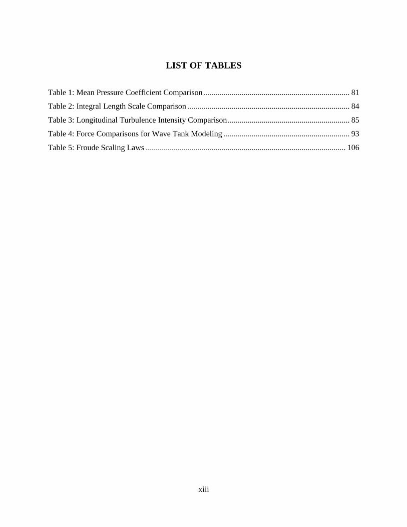
Table 1: Mean Pressure Coefficient Comparison ......................................................................... 81
Table 2: Integral Length Scale Comparison ................................................................................. 84
Table 3: Longitudinal Turbulence Intensity Comparison ............................................................. 85
Table 4: Force Comparisons for Wave Tank Modeling ............................................................... 93
Table 5: Froude Scaling Laws .................................................................................................... 106

xiv
LIST OF ABBREVIATIONS
ΔPmax Central pressure difference
𝜌 Density of water,
𝐴 Tributary area.
ACI American Concrete Institute
ADCIRC ADvanced CIRculation model for oceanic, coastal and estuarine waters
ASCE American Society of Civil Engineers
BLWT Boundary Layer Wind Tunnel
CAARC Commonwealth Advisory Aeronautical Research Council
𝐶𝑝 Pressure coefficient
CFD Computational Fluid Dynamics
CDF Cumulative Distribution Function
CTE Computational Tsunami Engineering
CWE Computational Wind Engineering
d Water depth or surge level
DAD Data Assisted Design
DL Dead Load
FEM Finite Element Model
FEMA Federal Emergency Management Agency
FFT Fast Fourier Transformation
FSI Fluid-Structure Interaction
g Acceleration due to gravity
𝐻s Significant Wave height,

xv
HDF Hierarchical Data Format
HURDAT HURricane DATabase
HAZUS HAZard US xvi
IBC International Building Code
LES Large Eddy Simulation
LL Live Load
LRFD Load and Resistance Factor Design
NCSU North Carolina State University
NDBC National Data Buoy Center
NIST National Institute of Standards and Technology
NOAA National Oceanic and Atmospheric Administration
NRL Naval Research Laboratory
NWS National Weather Service
ρw Density of water
PBE Performance Based Engineering
PBTE Performance Based Tsunami Engineering
PBWE Performance Based Wind Engineering
PEER Pacific Earthquake Engineering Research
PBEE Performance Based Earthquake Engineering
PD&E Project Development and Environment
PDF Probability Distribution Function
PSD Power Spectral Density
RANS Reynolds Average Navier Stokes

xvi
SDOF Single Degree of Freedom
SLOSH Sea, Lake Overland Surges from Hurricane
SWAN Simulation of Waves in Near Shore area
SWH Significant Wave Height
TWB Tsunami Wave Basin
OSU Oregon State University
UF University of Florida
UWO University of Western Ontario
Rmax Maximum hurricane radius
RPG Random Pulse Generation

CHAPTER ONE: INTRODUCTION
Tropical cyclones are intense low pressure storm systems that occur over the tropical
ocean, driven by the ocean‘s latent heat, mainly in late summer and autumn (Holmes, 2001).
The most intense and severe class of these cyclones develop in the Caribbean seas and are
termed hurricanes. Therefore, structures in coastal communities along the Atlantic and Gulf
Coast region are subject to the most severe nature of the numerous hazards that accompany these
storms. These hazards are not limited to the large wind gusts that are notorious to the event.
Intense storm surge and flooding have been shown to be the most damaging aspect to human life
and property.
Despite these hazards the population has grown in many of these communities, driven by
the moderate year round climate, theme park attractions and beautiful beaches. Due to the
increase in population in these areas, civil infrastructure has been constructed to accommodate
the public need. As a result, more structural systems have been exposed to these hazards such as
buildings, bridges, floodwalls (levees), dams and other coastal structures. Devastating
hurricanes such as Andrew or Katrina have shed light on the poor performance of the existing
design methodologies and codes, with numerous coastal infrastructure failures. According to
NIST report 1476, collaboration of over 26 experts from over 16 organizations including NIST,
FHWA and USACE recommends the establishment of a risk-based design methodology for
coastal structures, such as bridges.
A performance based design methodology integrates risk analysis alongside the standard
design objectives with a embedded goal of reducing loss to life and property. This shift requires
a more realistic prediction of the structural behavior of the system under a more accurate

18
description of the spectrum of loadings anticipated during the life-cycle. Therefore deterministic
based design conventions are to be replaced with a more scientifically oriented design approach
similar to the field of earthquake engineering. This approach is termed performance-based
hurricane engineering (PBHE).
However a distinct challenge is present in the implementation of such a methodology,
because the wind and wave hazards are distinctly different from earthquake hazards. The spatial
and temporal variation of the wind and wave loading is very drastic compared to earthquake
motion. Site-specific seismic ground motion records are typically applied to a structure‘s
foundation and spatial variation is not considered due to the rapid speed of seismic waves. On
the other hand, hurricane hazards, such as wind and waves are drastically different as the
structural configuration; orientations, and local site conditions all affect the loading distribution.
This phenomenon creates the need for a wealth of simulated pressure/force records from an array
of sensors placed all over the structure to take detailed readings during an extreme event.
However, each record is site and structure specific and must be performed for a vast array of
structures. Obviously, such an implementation is a drastic challenge to applying PBE.
Currently this void in this data has prevented widespread forecasting and damage
mitigation efforts (Masters, 2010). Only recently in 2010 with the formation Digital Hurricane
Consortium (DHC) has widespread collaboration among field activities have initiated in
developing such a database. Distinct challenges are present in instrumentation, regularity of
multiple platforms, and field logistics. Additionally three main contributions of uncertainty in
characterizing the wind field include: (i) inherent or aleatory uncertainty due to the unpredictable
nature of the wind velocity and magnitude, (ii) epistemic uncertainty due to incomplete or
19
missing data or information, and (iii) modeling uncertainty from estimating wind load effects on
structural response (Kiureghan and Ditlevesen, 2009).
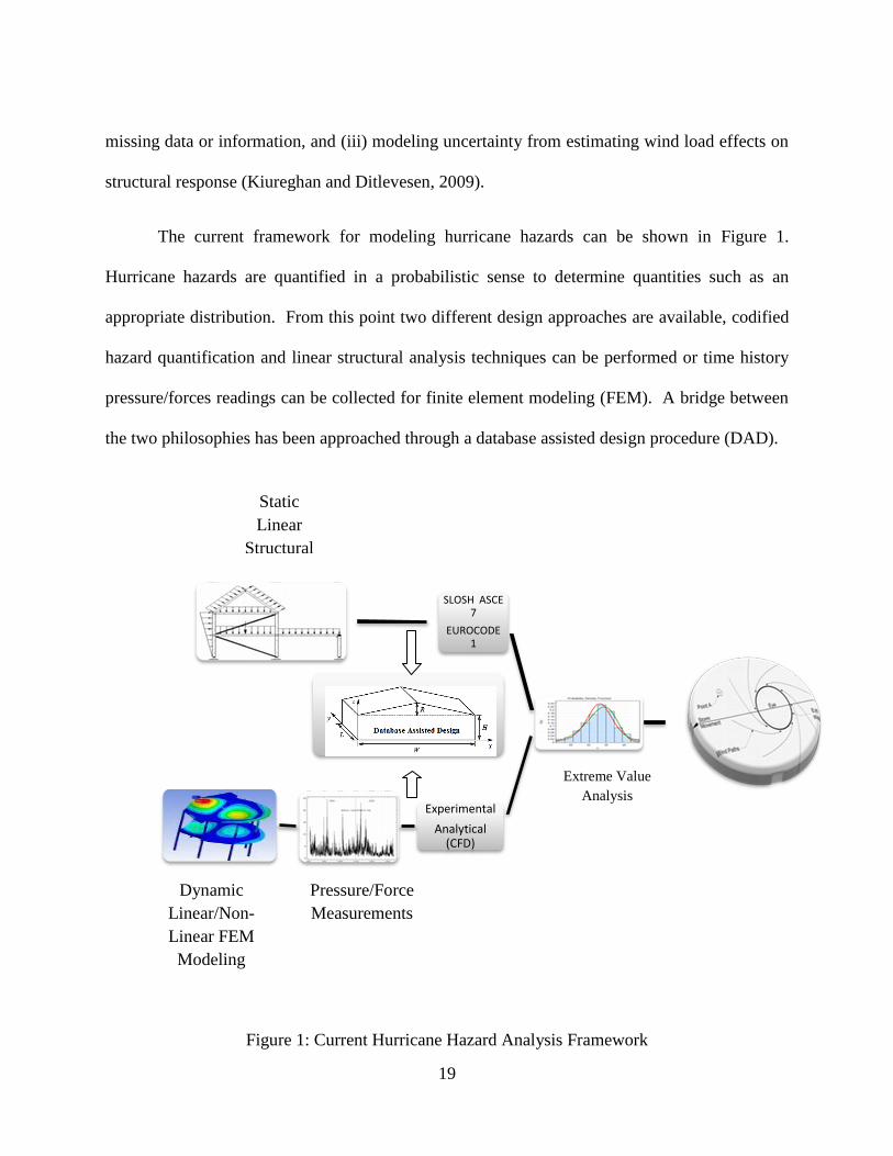
The current framework for modeling hurricane hazards can be shown in Figure 1.
Hurricane hazards are quantified in a probabilistic sense to determine quantities such as an
appropriate distribution. From this point two different design approaches are available, codified
hazard quantification and linear structural analysis techniques can be performed or time history
pressure/forces readings can be collected for finite element modeling (FEM). A bridge between
the two philosophies has been approached through a database assisted design procedure (DAD).
Figure 1: Current Hurricane Hazard Analysis Framework
SLOSH ASCE 7
EUROCODE 1
Experimental
Analytical (CFD)
Dynamic
Linear/Non-
Linear FEM
Modeling
Pressure/Force
Measurements
Static
Linear
Structural
Analysis
Extreme Value
Analysis

20
Therefore, in this study, an analytical method was undertaken to thoroughly investigate
the major hazards including wind and waves that accompany a hurricane event for several
structures. To quantify these hazards for PBE, a database of recorded data on simulated
hurricane hazards is required for structural analysis. However the resources for experimental
simulation of these multiple hazards are very limited and currently unavailable at the UCF
structures research facility at this time.
At the same time, the recent rise in computational hardware and computing power has
formed an efficient field of experimental research. Numerical simulations using computational
fluid dynamics (CFD) have risen in both the wind and wave engineering field, allowing more
cost effective multiple hazard research. The use of fluid structure interaction (FSI) software has
been validated in the aerospace and mechanical engineering fields for airfoils, racecars, and ship
design for 20 years. Only recently has the concept been extended in Civil Engineering FSI
problems such as wind and wave phenomena.
In this study, CFD simulations were to be carried out on several prototype structures to
thoroughly quantify the fluid hazards posed by a hurricane. Dynamic loads were to be generated
for comprehensive linear and non-linear structural evaluation. The Tampa Bay region was
selected due to the wide range of coastal structures and its susceptibility to Hurricane damage.
Before CFD simulations will be carried out on the prototype structures, verification of the
accuracy of the numerical simulation results is vital. Therefore, several records of laboratory
wind tunnel and wave tank basin experimental data were collected to verify the accuracy of this
tool. These verifications are a significant contribution as thorough comparisons shall continue to

21
enhance the confidence and warrant the practical use of CFD in structural design. Additionally
the widespread application of PBHE requires a versatile tool such as CFD
22
CHAPTER TWO: LITERATURE REVIEW
Numerous structural hazards are associated with hurricanes that accompany the storm
event. Identification and quantification of these extreme hazards are essential to application of a
performance based structural design. Performance based engineering design has been historically
applied to the field of earthquake engineering to assess hazards such as earthquake intensity or
liquefaction. However, the hazards that are associated with a hurricane can range from wind,
storm surge, waves and the potential for airborne or waterborne debris. Therefore in this study
the concept of PBE was extended in the hurricane engineering field.
Hurricane Hazards
Maximum Wind Speed
The classification of a tropical storm/cyclone into a hurricane is quantified through the
maximum wind speed. When the sustained maximum speed of the storm winds reach (33m/s,
74mph), the storm is officially classified as a hurricane according to the Saffir-Simpson scale.
These intense warm low pressure systems have an organized structure as shown in Figure 2
(Holmes). The Figure shows the circulation of the flow occurs with radial components toward
the ―eye‖ where a region of intense thermal convection causes air currents to spiral upward.
Outside the eye of the hurricane, the wind speed at the upper storm levels decays with radial
distance from the storm center. The gradient wind equation can therefore be used to determine
the wind speed at any radial distance from a storm center. The terms in the equation include the
Coriolios parameter (f), the radius from the storm center (r), the density of air (ρ), and the

23
atmospheric pressure (p). To apply the gradient wind equation a mathematical representation of
the pressure gradient such as the one proposed by Holland (1980) leads to Equation 1.
Figure 2: Structure of a Hurricane (Holmes, 2001)
Equation 1 describes the mean velocity field of an hurricane as a function of the radius to storm
center (r), the change in pressure across the storm (∆p), the characteristic scaling parameters A
and B, and Coriolis parameter (f).
(1)
To illustrate this effect, an anemometer reading 10m above the ground in a hurricane is
plotted in Figure 3. The Figure shows a period of very low recorded wind speeds as the eye of
the hurricane passed over this wind station and the wind direction changed nearly 180 degrees.
)r
Aexp(
r
AB
ρ
Δp
4
rf
2
rfU
BB
a
22

24
Also from the figure one can see the physical wind profile of a hurricane as the wind speed
decays from the eye of the storm.
Figure 3: Variation of Wind Speed/Direction at a point in a hurricane (Holmes, 2001)
The modeling and simulations of the natural wind flow phenomena around structures were
first studied using wind tunnels. Both aeroelastic and rigid scaled models equipped with
numerous transducers are commonly tested for fluctuating pressures induced by blowers or fans.
This technique has been validated in studies from surface pressure measurements on several
existing structures. One of these studies includes the Silsoe Structures building experiment
started in November 1990 by the UK Building Research Establishment. A large steel portal
frame building equipped with pressure taps and strain gauges to measure structural response
(Robertson, 1988). Results indicated for transverse flow from (0-180°), that accurate pressure
coefficients were obtained for both peak and time averaged values. Generally these
measurements justified the use of wind tunnel simulations for low-rise buildings.

25
However distinct challenges are still present in the use of wind tunnels in areas such as
similitude scaling. An exact equality of the kinematic, geometric and dynamic similarity
including Reynolds number and the Rossby Number for both prototype and model flows cannot
be obtained (Cermak, 1975). Conversely Reynolds number independence can be achieved for
these flow characteristics in a long wind tunnel composed of numerous roughness elements.
Different modeling techniques are typically employed in wind tunnel modeling such as the
high-frequency force balance technique which was first reported by Tschanz et al. (1983). The
method involves using a very rigid, high-frequency balance model system where only the
exterior surface of the structure is represented. Wind tunnel studies are then carried out on this
system and the overall fluctuating pressures are combined with the structural properties to
analytically determine the full-scale responses. Conversely, aero-elastc models involve
simulating the interaction between the motion of the structure and the aerodynamic forces.
Applications of this method typically include lightweight, deformable or lightly damped
structural systems where stationary models cannot accurately capture the potential additional
motion induced forces such as flutter.
Although structural failure rarely occurs from extreme wind speeds, a vast majority of the
structural wind damage occurs primarily to single family residential dwellings (Prevatt, 2009).
Wind damage to low rise buildings is primarily attributed to loss of the building envelope and
roof damage. Therefore researchers such as Simui et al. (2003) contend that the simplifications
of the current ASCE 7-05 analytical procedure can produce vast differences when compared to
experimental wind tunnel pressure fluctuation loads.

26
Storm Surge
Storm surge can be simply defined as the rise of water toward the shore by the force of the
wind swirling around an advancing storm (National Oceanic Atmospheric Adminstration-
NOAA). The surge created from the winds combines with the mean sea level to create a
hurricane storm tide.
Storm surge caused by hurricanes is one of the most devastating natural phenomena as nine
out of every ten hurricane related fatalities are attributed to storm surge (FEMA-456). Some of
the deadliest natural disasters in United States history occurred from storm surge waves
impacting coastal communities. The potential for this hazard is intensified today as much of the
Atlantic and Gulf Coast communities are densely populated and lie less than (4.5m, 15ft) above
the mean sea level.
Storm surge heights are affected by several variables including the timing of astronomical
tides, maximum wind speed and bathymetry of the ocean bottom. For example a steep drop from
the shoreline creates a deep pocket of water that reduces the storm surge effect but produces a
more powerful wave. Conversely, a long and gently sloping shoreline can produce higher storm
surges with small waves. Figure 4 displays this effect as the deep water reduces the energy of
the oncoming wave and allows that energy to dissipate.

27
Figure 4: Storm Surge Comparison Top: Shallow Coastal Slope Bottom: Steep Continental Shelf
Waves
Waves are typically generated in the deep water by the wind blowing across the surface.
Some of the key characteristics of waves are the height, wave length and wave period. In fluid
dynamics, the wave height of a surface wave is the difference between the elevations of a crest
and a neighboring trough. The wavelength is a measure of the horizontal distance between the
crest and trough, and the wave period is the time it takes for two consecutive crests or troughs to
pass a fixed point (Kinsmen, 1984). .
The waves that are generated during a hurricane are composed of a series of random waves
with various heights and periods. The height and period of these waves are affected by
numerous factors, including wind speeds; wind duration, fetch length and water depth.
Illustrations of the effect of some of these variables are shown in Figure 5. The fetch can be seen
as the distance over which a wind profile will travel before reaching the structure. From the

28
Figure, one can see that the increased duration of the wind has significantly increased the wave
height over time until they reach a state of a fully developed wave.
Figure 5: Fetch Length and Wind Duration Effects of Wind-generated waves (Sheppard, 2006)
Wave damage from hurricanes is significant and is most common in the coastal bridge
infrastructure. Recent Hurricanes including Hurricanes Ivan and Katrina, heavily damaged most
of the existing low-lying Gulf Coast concrete bridges. These bridges were subjected to the wave
forces of the hurricane as storm surge levels rose and inundated many of the bridges
superstructures.
Bridges are not the only structure affected by hurricanes as coastal buildings are also
subjected to wave forces due to the rising storm surge and tidal conditions. During a survey of
post-Katrina Hurricane damage, a number of failures of parking garages in flat slab, double-tee

29
and prestressed concrete floor systems resulted from the hydrodynamic uplift induced by the
surge and wave action (Robertson, 2007).
These detrimental effects have initiated numerous studies into the quantification of ―wave –
in-deck loads‖ which can be defined as hydraulic loads applied by waves to the deck or other
protruding elements (Cuomo, 2007). Laboratory wave tank basin facilities are currently the
accepted form of gathering wave-in-deck time dependent loads .
Researchers such as Sheppard et al. (2009) and Cuomo et al. (2007) have concluded that
wave-in-deck loads can be classified into two classes, Impact and Quasi-static. A specific
frequency or time period is not specified to distinguish the two categories, as the structure
properties affect the classification. Typically wave-in-deck loads can be classified as impact
loads if the load rise time is less than twice the resonant period for the mode related to the
applied load (Cuomo, 2007). Both characteristics are seen in a typical wave loading and thus the
time history is idealized as shown in Figure 6.
Figure 6: Idealized Wave Time History Superimposed of recorded signal from flume tests at HR
Wallingford, UK (Cuomo, 2007)

30
Scour
A secondary source of structural damage occurs to foundation systems during the recession
of a passing hurricane. Receding water flowing around the structure at a high rate may led to
erosion of the soils which support the foundation. The rate at which scour occurs depends
primarily upon the soil type. In addition to any storm or flood-induced erosion that occurs in the
general area, scour is generally limited to small, cone-shaped depressions. Localized scour
reduces the resistance of the foundation system by reducing its embedment. This reduction in
bearing capacity can readily cause the partial or total collapse of a coastal foundation.
The soil scour phenomena can occur as a shear or liquefaction-induced failure. The
liquefaction-induced scour is more ubiquitous during hurricane episodes (Robertson, 2008). The
soil matrix undergoes pore pressure change as the periodic wave action induces flow of the soil
particles below the foundation. This scour can then be intensified by the rapid drawdown of the
water in an inundated area as pore pressure changes are occurring much more rapidly.
Flooding
Flooding can occur during a hurricane event, both inland and along the coastal communities.
Inland flooding (typically termed flash flood) occurs from intense rainfall that in a very small
region over a relatively small time interval. Coastal flooding is typically created from a
combination of storm surge, oceanic tides, and rainfall.
Flooding has a variety of impacts on coastal buildings and their foundations, including
hydrostatic forces, hydrodynamic forces, flood borne debris forces, and erosion and scour. These

31
forces can dislodge buildings from their foundation with poor connections. Flooding is also a
major concern to emergency officials as it is the leading cause of fatalities during hurricanes.
Wind and Waterborne Debris
Wind Damage to structures is not limited only to the fluctuating surface pressures on the
building envelope but flying debris that are generated in the wind field also. These airborne
missiles have the possibility of striking the structure and penetrating the building envelope. The
loss of the building enclosure can lead to undesirable consequences like high internal pressures,
additional debris and water damage (Holmes, 2001).
Waterborne debris can be produced during flood events and can include a variety of objects.
The potential for waterborne debris has been mapped in specific regions as determined by the
ASCE. The waterborne debris region is defined as areas within hurricane-prone regions within
one mile of the coastal mean-high-water line where the basic wind speed is (49 m/s, 110mph).
Wind and waterborne debris are not as widespread as other hazards that are associated with
the hurricane event and are therefore not as thoroughly quantified. One empirical formula is
provided by ASCE 7 for impact forces. In Equation 2, the impact force (F) is given by the
weight of the object (w), impact velocity (v), acceleration of gravity (g) and the impact duration
(∆t) (typically 0.03-0.3 sec).
(2) tg
wv
2F

32
However, the location and time varying aspect of this loading phenomenon is not fully
understood and is rarely accounted for in structural design. Additionally, according to a survey
of post-Katrina coastal damage, very few structures were damaged by debris from the storm
(Robertson, 2008).
Quantification of Hurricane Hazards
Some effort has been made to quantify the hazards that are associated with hurricane events.
The Saffir-Simpson Scale was formulated in 1969 by Herbert Saffir, a consulting engineer, and
Dr. Bob Simpson, Director of the National Hurricane Center. The need for the scale was
founded on the principle of communicating the gradations of risk that are associated with
hurricanes that may allow emergency officials to better manage these disasters. Although the
scale is based on physical observations of wind damage and storm surge events seen in
hurricanes, the rating of a storm is highly subjective and is not a definitive probabilistic quantity.
Due to the non-uniform nature of the hurricane structure, a single category rating for the entire
storm will yield inaccurate results. Thus, the application of the Saffir-Simpson scale in PBE is
very limited but it is a useful tool in describing the potential hazards associated with the intensity
of the storm.

33
Figure 7: Saffir-Simpson Scale (National Weather Service)
Performance Based Engineering
Performance based structural engineering entails analyzing structures under the extreme
hazards identified to achieve better performance or protection. The response of the structure is
not only termed in states of failure and safe, as the case with conventional Load and Resistance
Factor Design Method (LRFD), but all spectrums of the response are quantified, including states
such as safe, partially safe and unsafe. This shift requires a more realistic prediction of the
structural behavior of the system under a more accurate description of the spectrum of loadings
anticipated during the life-cycle. The need for this change in design methodology arose from the
prescriptive nature of current design codes and the desire for more accurate design methodology.
These codes contain minimum standards of care (and performance) and no information on how

34
to achieve better performance or protection against manmade or natural hazards (Whittaker,
2005). The current codes in practice including ASCE 7 and International Building Code (IBC)
are only reviewed following a disastrous event and are based on judgments by distinguished
design professionals as to whether the losses were acceptable, given the severity of the event.
This lack of quantitative evaluation of the performance of the structures gives very inaccurate
conclusions on the state of the design community. Therefore it is believed that the development
of performance-based engineering tools for extreme loadings on structures will improve out civil
infrastructure. PBE was first applied to earthquake engineering but, it has been extended into
other extreme hazards both manmade and natural including blast, fire, hurricanes, and tornadoes.
An example framework of the PBE methodology has been outlined by the Pacific
Earthquake Engineering Research (PEER). A typical PBE assessment approach is a four step
procedure that first involves identifying all potential hazards in a more scientifically oriented
procedure called Hazard Analysis. Next, the structure is analyzed under the given hazards in
Structural Analysis to determine demand parameters, such as the story drift. According to the
specific building type and arrangement, the structural response can be mapped to the damage
potential in Damage Analysis. Once the damages of the structure have been determined, the
Losses of the structure can be quantified in terms of loss of time, money and life in Loss
Analysis.

35
Performance-Based Hurricane Engineering
Performance based hurricane engineering (PBHE) is a relatively active field of research.
Currently, most of the work in PBHE has been focused on specific hazards that are associated
with the hurricane event, and no current experimental research has been conducted on the
combined effects of hurricanes including wind and hydrostatic and hydrodynamic forces.
Numerous studies are currently active in investigating these loads through both numerical and
experimental measures.
Numerous studies have been conducted on designing structures due to wind loads in a
performance based manner. Some of these studies include Sibilio and Ciampoli et al. (2007) in
which advanced Monte Carlo simulation was carried out on a footbridge subjected to turbulent
wind. Norton et al. (2007) presented an efficient method for analyzing structures under
hurricanes loads for tall buildings. Ongoing research at the University of Florida has been
focused on both full and 1/3 scale residential structures composed of wood subjected to the UF
Hurricane Simulator (Prevatt, 2009).
Another field of PBHE is in the field of wave and storm surge effects to structures termed
as Performance Based Tsunami Engineering (PBTE). Waves are generated by both tsunamis and
hurricanes, which have been shown to have devastating effects to life and property. Currently
engineers have little to no guidance to when designing structures in wave prone areas (Yim,
2009). However numerous studies have been recently conducted on the wave effects on
structures.

36
Some of this research includes work from Cuomo et al. (2007) in which guidance for
hydraulic loads for bridge decks were given from wave flume tests at HR Wallingford in the UK.
Shepperd et al. (2009) developed a theoretical wave force models from a wide range of wave
conditions from 1200 wave basin tests. Ongoing research at the Tsunami Wave Basin (TWB) is
being performed to investigate the response of residential structures by subjecting scaled 1/6
models. Wave Induced forces are measured for different building configurations to see the
change in the wave- induced loads (Yim, 2009).
Database Assisted Design (DAD)
A Database Assisted Design methodology implements directional time history data of
experimental pressure coefficients obtained from wind tunnel testing for use in the design and
analysis of structures (Main and Fritz, 2006). The first step in building a DAD program is the
collection of a plethora of wind tunnel data for various wind angles and surface terrain
conditions.
One such application of the DAD procedure was in the development of a MATLAB
program named WINDPRESSURE (Main and Fritz, 2006). The program provides a graphical
user interface that develops structural responses such as internal bending moment and deflection
that can allow the performance of the structure to be assessed. The DAD program then utilizes
an interpolation algorithm to allow for mapping of tested building models to any building
dimensions. Therefore once developed any building of similar structural orientation and
arrangement may be designed to achieve better performance.

37
Storm Surge Models
The ability to accurately predict the estimated levels of storm surge and waves
anticipated from a given hurricane event is crucial for emergency officials and design engineers.
Several computer generated surge and wave prediction models are currently available. Currently
two commonly used packages are Sea, Lake Overland Surges from Hurricane (SLOSH) and
ADvanced coastal CIRCulation and storm surge modeling (ADCIRC).
ADCIRC is based on solving the time dependent, free surface circulation and transport
problems in two and three dimensions. Typical ADCIRC applications have included everything
from analysis of hurricane storm surge and flooding to dredging and material disposal studies.
One study coupled the ADCIRC (ADvanced CIRCulation) surge model and the SWAN
(Simulation of Waves in Near shore areas) wave models. The team simulated the storm surge
and wind waves generated by Hurricane Katrina on the Mississippi and Alabama coasts for
developing a theoretical wave equation for bridge decks (Douglass, 2006).
A government created surge model commonly used by FEMA officials is named SLOSH,
which was created by the National Weather Service (NWS). SLOSH is two-dimensional,
numerical and dynamic storm surge modelers that can be used to develop real time estimates of
storm surge levels generated from Hurricanes, by taking into account a storm's pressure, size,
forward speed, forecast track, wind speeds, and topographical data. SLOSH is not considered a
predictive tool as the track of the hurricane at landfall must be known for accurate simulation of
the storm surge. The SLOSH program divides the US Atlantic and Gulf Coasts into 41 basins,
which are further subdivided into smaller polar coordinate grids that allow for more accurate
refinement of each basin. Using these refined grid meshes the individual elements of the

38
SLOSH grid are the basis for calculating the water surface elevations caused by storm surge in a
specific SLOSH basin. The transport equations of motion are used for calculating the storm
surge in the SLOSH models (Jelesnianski, 1992).
Computational Fluid Dynamics (CFD)
Computational Fluid Dynamics is a subset of fluid mechanics in which numerical
methods and algorithms are utilized to solve and analyze fluid flow problems. The basis of all
CFD modeling packages is the use of the Navier-Stokes equations of fluid flow. A system of
nonlinear partial differential equations of second order defines the conservations of mass,
impulse and energy of a three-dimensional fluid flow. Solution techniques include finite element,
finite volume and spectral analysis.
CFD modeling typically has been applied in the field of mechanical and aerospace
engineering. Airfoils, spacecraft, racecars and other high rate traveling mechanical machinery
have been simulated both in small scale wind tunnels and CFD modeling packages. Numerical
simulations reduce the overall cost of conducting real world experiments, making it a very active
field of research. More recently, this computational power has been actively researched in the
structural engineering field. Extreme structural loads such as wind, waves, blast and impact have
been modeled using CFD techniques. Specifically, research in the wind and wave engineering
community began in the late 1980‘s in which simulations of fluid flow interaction with structures
is conducted. Today increased computer performance has stimulated this research and a specific
field of computational wind and tsunami engineering has been developed.

39
Computational Wind Engineering (CWE)
The application of CFD in wind engineering is termed computational wind engineering.
This field of research is still very limited in its widespread use, but it has seen a recent rise in
interest. Hardware and software capabilities have increased tremendously since CWE‘s
inception in the late 1980‘s. This has led to significant progress toward application of CWE to
evaluate wind loads on buildings. Some countries such as Japan have established methods for
assessing pedestrian wind levels using Reynolds Averaged Navier Stokes equations (RANS) and
Large Eddy Simulation (LES) (Dagnew, 2009).
RANS and LES turbulence modeling approaches are typically performed in any CFD
modeling application to reduce computational demand. Direct solution of the Navier-Stokes
equations requires very fine grids to accurately capture all turbulence scales in the flows and is
not applicable to typical Reynolds numbers encountered in wind engineering (Franke, 2004).
LES involves solving the time-dependent fluid equations on a coarse grid which removes the
small scale turbulence of the flow. The RANS modeling approach employs turbulence models to
the averaged equations to directly yield the steady state solution of the flow variables (Franke,
2004). The RANS modeling approach is the most common approach used in CWE.
As stated by Dr. Dagnew from Florida International University (FIU) that ―at this stage in
the CWE community, a systematic validation of CWE models through comparison with wind
tunnel experiments will enhance the confidence and warrant its use for practical applications.‖
Thus, numerous researchers from around the nation are working on improving this technique and
validating its precision. Ganeshan (2009) presented LES simulation coefficient of drag
comparisons for stack interface applications. Numerical wind loading pressures developed on a

40
basic cube were investigated in studies by (Stathopoulous, 2002) and (Lim, 2009). Some of the
computational efforts that have devoted to tall buildings include Huang et al (2007) and Braun et
al. (2009) in which flow patterns and both mean and RMS pressure coefficients were compared.
A thorough comparison of pressure coefficients obtained from both experimental wind tunnel
tests and a Commonwealth Advisory Aeronautical Council (CAARC) were presented in Dagnew
et al. 2009. Wind tunnel results from 1:400 scale rigid models tested were compared against
RANS modeling of the CAARC building model. Figure 8 shows a comparison of the
computational dimensions and fluid boundary conditions to the wind tunnel test setup. Results
of this study showed good agreement between the CAARC numerical simulation and the wind
tunnel mean pressure coefficients. An example of the pressure coefficients at various points on
the building are shown in Figure 9. Also included in the plot are other researchers work on the
same data collected including Braun (2009) and Huang (2007). Pressure coefficient comparisons
deteriorate slightly at the sidewalls but improve at the leeward wall (Dagnew, 2009). The shapes
of the plots are very similar to a horseshoe vortex shape contour generated along the windward
face that agrees with the wind tunnel simulations.

41
Figure 8: A.)CAARC building computational building domain and boundary conditions B.)
Wind Tunnnel Configuration (Dagnew, 2009)
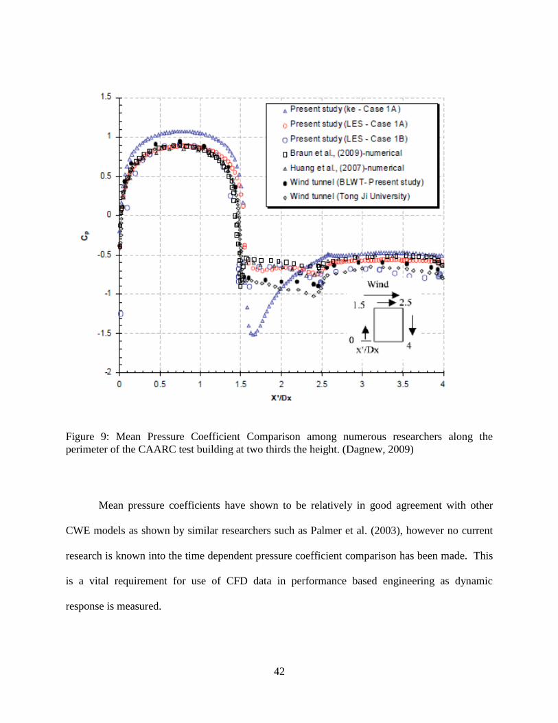
42
Figure 9: Mean Pressure Coefficient Comparison among numerous researchers along the
perimeter of the CAARC test building at two thirds the height. (Dagnew, 2009)
Mean pressure coefficients have shown to be relatively in good agreement with other
CWE models as shown by similar researchers such as Palmer et al. (2003), however no current
research is known into the time dependent pressure coefficient comparison has been made. This
is a vital requirement for use of CFD data in performance based engineering as dynamic
response is measured.

43
Computational Tsunami Engineering (CTE)
The application of CFD techniques are also currently being researched in the field of
coastal engineering. The application of CFD to Tsunamis is termed Computational Tsunami
Engineering. Similar to CWE research, CTE is a very innovative field and only a select few
Universities are conducting such research. As discussed previously, the TWB at OSU was
constructed to further understand the dynamic interactions of tsunamis and structures. Also
computational efforts are being conducted on the use of CFD modeling for predicting the wave
forces generated during tsunamis or hurricanes.
One such study included single setup waves impacting a cylinder in the TWB. Impact
forces were compared with CFD numerical model simulations, using the software LS-DYNA
(Yim, 2009). This work was performed as a preliminary check to address the validity of the
numerical simulation. Comparisons of the two methods are shown in Figure 10. Very good
agreement is seen between the CFD models and the TWB experimental data. Additionally, wave
surface pressures are also estimated for various depths using the LS-DYNA simulation. This
study confirmed that the possibility of CFD modeling of extreme wave forces from tsunamis or
hurricane-generated waves is feasible.

44
Figure 10: Comparison of numerical and experimental wave amplitude and surface pressure time
histories. (Yim, 2009)
MSC DYTRAN
Dytran is an explicit finite element analysis (FEA) software with the ability to solve a
variety of highly complex non-linear structural analysis problems (Dytran, 2008). Most FEA
programs implement implicit methods to carry out transient solutions using a Newmark iteration
technique to integrate forward in time (Dytran, 2008). Explicit methods typically employ a
central difference scheme to advance in time (Dytran, 2008). Explicit methods are particularly
suitable if the time step required for problem is very small. Some example problems requiring
such small iteration steps include very large material nonlinearity, geometric non-linearity such

45
as friction, or problems containing physics demands such as stress wave formulation (Dytran,
2008). Therefore for models containing a high number of elements and notable material
nonlinearity, then explicit methods provide more efficient solution technique as they do not
require the costly formulation and decomposition of matrices each time step. Instead the typical
sequence of each time step loop is carried out as shown in Figure 11. However other
commercially available CFD programs such as FLUENT, employ both implicit and explicit
techniques for FSI simulations. Implicit methods are suitable for steady state results as large
time steps introduce truncation error of the independent variables.
Figure 11: Explicit time stepping method for Dytran (Dytran Users Manual, 2008)
One of the main features of Dytran is the ability to model fluid-structure interaction
problems. This feature is accomplished through the use of two separate descriptions of motion.

46
This step is an important consideration for simulating flow problems using numerical methods as
the choice of an appropriate kinematical description of the flow field can affect the accuracy and
stability of the results (Donea and Huerta, 2003). The algorithms of continuum mechanics make
use of three distinct types of description of motion: the Lagrangian, the Eulerian and the ALE
description. Dytran employs both Eulerian and Lagrangian descriptions to model both fluid and
structure motion. A short illustrative description of each technique is provided below.
The Lagrangian formulation is utilized in Dytran for the motion of elements with a
constant mass such as rigid structural materials. The motion of the material points, relate the
material coordinates (X), to the spatial coordinates (x) by mapping υ. Therefore during any time
interval the link between X and x can be described by the law of motion. Due to the one to one
mapping υ and since material points coincide with the same grid points during motion, the free
surfaces and interfaces between materials is tracked easily through the inverse transformation
(Donea and Huerta, 2003). Therefore the material is collected into a mesh, and as the body
deforms each grid point moves with the material and the element distorts (Dytran, 2008).
However, when large deformations occur such as vortices in fluids, Lagragian applications may
be unable perform such calculations or even result in large errors (Donea and Huerta, 2003).
Conversely, the Eulerian meshes are in a fixed reference frame in space and the
continuum moves and deforms with respect to the computational grid. Conservation equations
are formulated for variables and functions having an instantaneous significance in a specific
fixed region (Donea and Huerta, 2003). This formulation therefore disassociates the mesh nodes
from the material particles and introduces convective terms. This result enables the treatment of
complex material motion but, introduces difficulties in tracking the material interfaces and
boundaries. Thus the Eulerian Solver is utilized in Dytran for modeling fluids or materials that

47
undergo large deformations. Under this technique, the material of a body under analysis moves
through the Eulerian mesh, as the mass, momentum, and energy of the material are transported
from element to element (Dytran, 2008). Additionally, through the use of the dynamic viscosity
term in modeling of Eulerian elements, the use of Navier-Stokes Equations is executed for the
fluid domain.
The ability of any FSI simulation is made possible through the use of a coupling
algorithm where both materials can interact In Dytran, both the Eulerian and Lagrangian meshes
can be combined in the same computation through the use of a general coupling surface or
Arbitrary Lagrangian-Eulerian (ALE) coupling surface. This surface acts as a boundary to the
flow of material in the Eulerian mesh. The stresses in the Eulerian material then exert forces on
the surface of the Lagrangian mesh, causing those elements to distort. However, the fluid
response is also a function of the structures‘ surface motion requiring a feedback loop to be
executed each time step (Donea and Huerta, 2003). The general coupling surface is used when
fluid displacements are small and linear elastic structures are used. Conversely the ALE
formulation is recommended to model nonlinear fluid interaction with nonlinear structural
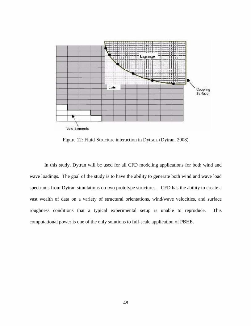
elements. A visual representation of the setup of FSI in Dytran is seen in Figure 12.
48
Figure 12: Fluid-Structure interaction in Dytran. (Dytran, 2008)
In this study, Dytran will be used for all CFD modeling applications for both wind and
wave loadings. The goal of the study is to have the ability to generate both wind and wave load
spectrums from Dytran simulations on two prototype structures. CFD has the ability to create a
vast wealth of data on a variety of structural orientations, wind/wave velocities, and surface
roughness conditions that a typical experimental setup is unable to reproduce. This
computational power is one of the only solutions to full-scale application of PBHE.

49
CHAPTER THREE: METHODOLGY
In this study, a thorough investigation of hurricane hazards was performed using
computational simulations. Numerous hazards associated with a hurricane event were reviewed
including primary and secondary effects. However, due to wide scope and range of hurricane
hazards, only the most probable effects that a typical structure experiences will be investigated.
These hazards typically include extreme wind speeds, storm surge and the hydrodynamic forces
from waves.
The first step in applying CFD to modeling hazards such as wind was to verify the
accuracy of the results obtained through these simulations. This was performed by collecting
existing experimental data from full scale laboratory experiments and comparing the time
dependent forces/pressures to those predicted from the CFD analysis. Once the models were
verified, prototype simulations were performed on bridge and building structures. Once dynamic
time history loads were generated structural FEM models were carried out to demonstrate
demand analysis on prototype structures. This process is shown in Figure 13.
Figure 13: Research Methodology
Verification Studies
Protototype Structures
Structural FEM Models

50
Verification Studies
To validate the use of Dytran for PBHE, both wind tunnel experiments and wave tank
basin experimental data was collected. Information regarding the experiment setup, atmospheric
conditions, boundary conditions and data collection devices was recorded to enable the
reproduction these experiments numerically. This will enable signal comparisons to be
conducted using digital signal processing techniques and structural analysis techniques.
Wind Tunnel Validation
The wind tunnel data utilized in this study was collected at the UWO BLWT. These wind
tunnel time histories were presented in Ho et al. (2005) and were utilized in the development of
WINDPRESSURE. A total of eight different tests were run on different building configurations
for various wind angles. During each test, a series of various pressure taps recorded the wind
pressure distribution on the model. Due to time constraints and the scope of this study only one
building configuration was used for numerical validation.
The building configuration chosen is a typical gabled structure. The model consisted of a
1:100 scale structure with dimensions (57 X 36.5 X 5.5 X 1.5 m, 187.5 X 120 X 18 X 5 ft
(Length X Width X Eave Height X Rise). This building was placed in the UWO short wind
tunnel equipped with approximately 4000 pressure taps sampled at 500 Hz for 100 seconds.
Pictures of the building and experimental setup are shown in Figure 14.

51
Figure 14: Photos of Building Model in UWO wind tunnel. (WINDPRESSURE, 2005)
Consequently, the exact building was replicated using LES in Dytran. The same 1:100
scale model was made with 424 Lagragian shell elements made of an Elasto-Plastic steel
material (DMATEP). However, the model was constructed to be effectively rigid by defining a
thick shell for the structure. The boundary layer atmosphere was constructed with over 13,000
Eulerian quadrilateral solid elements (CHEXA). Figure 15 shows both the Eulerian and
Lagragian Mesh of the CFD model used for wind tunnel verification. The initial properties of
the air that were input in the program are the initial velocity, internal pressure, specific internal
energy, dynamic viscosity, and density. Information regarding many of these properties is
standardized for room temperature and only the initial velocity state of the material was
assumed, and the specific internal energy was set to zero. The initial velocity was set to zero to
simulate stagnant conditions in the wind tunnel. The specific internal energy of the air was set to
zero to eliminate the gamma gas law. Boundary conditions on the Eulerian mesh were set to
simulate the actual wind tunnel test. Air flow was initiated by air entering one side of the

52
Eulerian mesh and exiting on the opposite boundary. Only a constant wind speed can be input
into the DYTRAN simulation and therefore several surface roughness elements were created
upstream of the building model to create more turbulence in the numerical simulation. However,
due to computational resources and time constraints, extensive use of roughness elements in the
CFD models was unfeasible. These elements drastically increase the number of elements in both
the Lagragian and Eulerian mesh and severely increase calculation time. In order to simulate the
roughness introduced in the wind tunnel experiment, element faces of the Eulerian mesh were
simulated as barriers whereby no flow of material is allowed. Several rows of these elements
were added to introduce time varying vortices to develop a more time varying response. These
barriers are seen in Figure 15 as well.
A coupling algorithm was utilized in DYTRAN to enable the complex fluid-structure
interaction. Additionally, to simulate the effect of the frictional resistance provided by the
structure as the fluid is flowing around it, a skin friction coefficient is input in DYTRAN. The
skin friction coefficients can be derived from the drag coefficient, which depends primarily on
the Reynolds number. A reasonable estimate of the drag coefficient for the Reynolds number for
this simulation of 6e105 can be taken as 1.2, which is equivalent to a frictional coefficient in
Dytran of 0.095.

53
Figure 15: CFD model from DYTRAN of UWO experiment. Blue: Eulerian Elements (Fluid)
White: Lagragian Elements (Structure)
One of the main benefits of the numerical simulation technique is the wealth of available data
to be collected during the experiment. In this study, nodal force time histories for X, Y, Z and
resultant components and Eulerian mesh parameters were recorded at a sampling rate of 500Hz.
In the numerical models, a record of each nodes force time history can be recorded and
converted to a pressure coefficient through the tributary area of each node. This will enable
direct comparison with the wind tunnel pressure tap data. A typical CFD model was run for a
10 second duration at a sampling rate of 500Hz generating 1.5-2 GB of data. These models were
run on a single core Pentium four processor, to generate the ten second duration worth of data
and required 112 hours in simulation time. Due to these high computational costs, only two
wind directions were used for validation with the wind tunnel. In the wind tunnel experiments,
Air
Flow
In
Air Flow
Out

54
models were rotated on a turntable to create the various angles of the wind attack. In the
DYTRAN simulation, general coupling requires the meshes to be aligned in the Cartesian
coordinate plane. Therefore, in the DYTRAN simulations the velocity of the air is given their
respective component values, based on the angle of attack. The angle of attack that was chosen
for comparison was 75 and 45 degrees from the longitudinal axis of the building, or 15 and 45
degrees transversely respectively.
To ensure that all effects of the wind pressure distribution are captured throughout the
building, CFD comparisons will be conducted for five separate locations of the building. The
five locations used in the comparisons will be: windward wall, windward roof, leeward walls,
leeward roof, and roof peak. On each face, a node from DYTRAN was selected and a
corresponding pressure transducer from the wind tunnel experiment was sampled for direct
comparison. For each node, a time varying force was captured in Dytran that could be converted
to pressure through its tributary area. A list of the comparisons included: mean pressure
coefficient, power spectral density (PSD), autocorrelation, integral length scale, and the
turbulence intensity. An outline of each measure will be made in the next section.
Mean Pressure Coefficient
During wind tunnel testing experiments, measured external pressures are typically stored in a
non-dimensional form known as pressure coefficients (Cp), as shown in Equation 3. The
measured pressure, (P) is normalized by the air density, (ρ) and the mean wind velocity at roof

55
height, (V) to obtain the pressure coefficient. From this parameter, wind pressures for any
particular speed can be obtained by appropriate scaling.
𝑃 =1
2𝜌𝑉2𝐶𝑝 (3)
Internal pressures develop in a model due to the openings in the building envelope and other
leakage paths. Fluctuating internal pressures are not measured in wind tunnels directly however
they can be determined through an empirical relationship given in Devenport et al. (2007) from
the external pressures. Therefore the net load on the cladding can be determined as the difference
between the internal and external pressures. This information is used for determining design
pressures for cladding and glazing components of buildings.
Data provided from the wind tunnel experiments at the UWO laboratory were given in the
pressure coefficient form. However, in the CFD simulation Dytran generates force
measurements that were converted to a pressure using each nodes tributary area. The velocity at
the boundary was defined as (26.831m/s, 60mph) but this velocity is not the velocity seen at the
mean roof height, when the air interacts with the structure. No measurements of wind velocity
are taken during the simulations on the building however, the Eulerian mesh was inspected to
observe the wind velocity. This value was found to be around (17.1m/s, 56.1ft/s) at the roofline
and was used for all calculations.
Another important characteristic for comparing mean pressure coefficients is to ensure that
averaging time is consistent, as described by Main and Fritz (2006). ASCE 7-05 uses pressure
56
coefficients derived from a 3 second gust at (10m, 33ft) above ground in current design
standards. However, due to the model and prototype scaling, wind tunnel mean pressure
coefficients are derived under a time window of approximately 1 hour (once converted to
prototype scale) (Main and Fritz, 2006). During the verification studies as discussed previously
Dytran mean pressure coefficients were derived from a ten second signal due to the high
computational demands.
Power Spectral Density (PSD)
The power spectral density (PSD) of a random process describes the power distributions of
the signal in the frequency domain. Thus it shows at which frequencies variations are strong and
at which frequencies variations are weak. Mathematically, it is defined as twice the Fourier
Transform of the autocorrelation sequence of the time series, or the squared value of the Fourier
transform of the time series as shown in Equation 4.
𝑆𝑢(𝑛) = lim𝑇→∞ 2
𝑇 𝑋𝑇(𝑛)
2 (4)
Simiu and Scanlan (1996) showed that the spectral density of the signal can be used to
describe the energy spectrum of the turbulent motion (Yu, 2008). Turbulent energy fluctuations
on the building can be seen as the superposition of numerous winds eddies that combines and
contributes to the total kinetic energy. Each eddy is characterized by a periodic motion of
circular frequency (𝜔 = 2𝜋n) or wave number (λ) (Yu, 2008).

57
Thus, to ensure that Dytran has captured all turbulent eddy contributions of the wind, a PSD
was then computed for both signals and compared. To smooth the PSD plot a Hamming window
was applied to a Welch PSD (Yu, 2008). This method is based on the direct Fast Fourier
Transform (FFT), which was implemented in MATLAB. The plots were then normalized by the
standard deviation of the longitudinal wind component (σu), Integral Length scale (Lux) and the
mean wind speed (U). Due to both positive and negative deviations, the value is first squared
and before averaging them, and finally the root is taken to given consistent wind speed units.
Mathematically the formula for the standard deviation can be found in Equation 5.
(5)
Additionally, to ensure accuracy in both numerical and experimental wind modeling
techniques, the respective spectra was compared against established methods for estimating the
spectrum for design purposes. These established methods include Von Karman, Eurocode I and
Busch and Panofsky et al. (1968) (Holmes, 2001).
Autocorrelation
Autocorrelation is a statistical tool used to measure the correlation of two values in the same
data set at different time steps. The autocorrelation coefficient can detect non-randomness in data
2
1
0
2])([1
T
u dtutuT

58
as it is closely related to the spectral density. The autocorrelation coefficient is also used in
calculation of the integral length scale.
The calculation of the autocorrelation function is shown in Equation 6 where T is defined as
the length of time for the record and τ is defined as the time lag.
According to Yu et al. (2008), the autocorrelation coefficient/function and integral length
scale are affected by the length of record being analyzed (Yu, 2008). Therefore, for the
autocorrelation comparison, only ten seconds of data from both the wind tunnel and CFD
simulations will be used.
.
(6)
Integral Length Scale
Another measure of the turbulence of the signal is the calculation of the integral length scale.
The integral length scales of turbulence are measures of the average size of the turbulent eddies
of flow. There are 9 scales corresponding to the three dimensions and three types of eddies
(longitudinal, transverse and vertical). According to Simiu and Scanlan (1996), the integral
length scale can be calculated according to Equation 7 where U is the mean wind speed, τ is the
time lag, ū2
is the longitudinal turbulence fluctuation and ρuu is the autocorrelation coefficient.
The longitudinal turbulence fluctuation is based on an empirical constant β and squared value of
the friction velocity.
T
TTxx dttxtxR )()()( lim

59
(7)
Turbulence Intensity
One of the most straightforward characteristics of the atmosphere‘s turbulence is described
in a quantity termed the turbulence intensity. The turbulence intensity is defined mathematically
as the ratio of the standard deviation of each fluctuating wind speed component to its mean
value. Typically for wind observations, the time window used for the calculation is between 10
minutes and 1 hour (Simiu and Scanlan, 1996). For our DYTRAN simulations, the ten second
record will be used for this calculation.
The turbulence intensity is also compared against an approximate relationship given in
Holmes (2001). Through measurements of surface wind gusts produced by large scale
depression systems, the turbulence intensity can be approximated through Equation 8.
Therefore, the turbulence intensity is entirely characterized by the surface roughness length of
the terrain (zo).
(8)
0
2)(L d
u
Uu uu
x
oo
u
z
z
z
zu
uI
ln
1
ln4.0
*
*5.2

60
Single Degree Of Freedom Response (SDOF)
The last verification method used was to validate the use of CFD simulations from a dynamic
response instead of a static comparison. As stated in the literature review this is critical for the
use of CFD in PBHE, as little research has been committed to this topic in the CWE field.
Additionally Dytran is typically performed for sudden transient impulses and well developed
turbulence models for LES simulations may not be employed. These applications typically
include impact, ballistic or other short duration loading situations. These time durations
typically are on the order of milliseconds or tenths of seconds. However, for wind tunnel
comparisons the CFD simulations were ran for 10 seconds. In order to ensure that the dynamic
response of a system is not lost in the numerical simulation the response of a single degree of
freedom (SDOF) system was investigated.
A program in MATHCAD was used to analyze a time dependent force input on a SDOF
system with damping, according to the average acceleration method. The SDOF system was
defined with a mass of (500kg, 1,100lb) which when scaled to model dimensions represents 110
kip and a natural frequency of 5Hz. The damping of the system was set to 5% of the critical
damping. Due to the large wealth of collected data in 100 sec at 500 Hz (50,000 data points),
only 10 seconds of the wind tunnel record was used and then the load was released for a total
recording of 13 seconds. This was mimicked with the CFD simulation data, and comparisons
were made of the displacement, velocity and acceleration of the SDOF system for all thirteen
seconds. Finally, power spectral analysis of the response for each method was compared to
verify the frequency content of the dynamic response.

61
Wave Tank Verification
For this study, wave basin records from studies conducted at the Coastal Engineering
Facility at the University of Florida were collected (Shepperd, 2009). Using a wave tank
measuring (1.8m, 6ft) wide by (1.8m, 6ft) tall and (36.5m, 120ft) in length numerous bridge
configurations of various levels of complexity were investigated. In all, over 1100 tests were
performed for numerous wave periods, wave heights, structure clearance height, and structural
models (Sheppard, 2009).
The models used in the study were built from scale 1:8 replica of the I-10 Escambia Bay
Bridge. This bridge experienced failure during Hurricane Ivan, as many of the segmented spans
were pushed off their pier caps and into the bay, from the storm inundation and hydrodynamic
wave forces. Figure 16 shows the progression of structural elements added to the bridge models
to help quantify the effects of the wave forces on bridges. The First Model (A) only represents
the slab of the bridge and further models continue to add the girders, overhang, and crash barriers
(B-D).
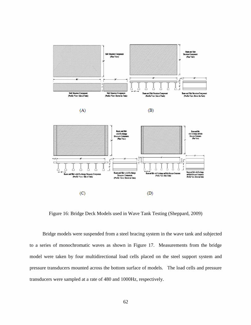
62
Figure 16: Bridge Deck Models used in Wave Tank Testing (Sheppard, 2009)
Bridge models were suspended from a steel bracing system in the wave tank and subjected
to a series of monochromatic waves as shown in Figure 17. Measurements from the bridge
model were taken by four multidirectional load cells placed on the steel support system and
pressure transducers mounted across the bottom surface of models. The load cells and pressure
transducers were sampled at a rate of 480 and 1000Hz, respectively.
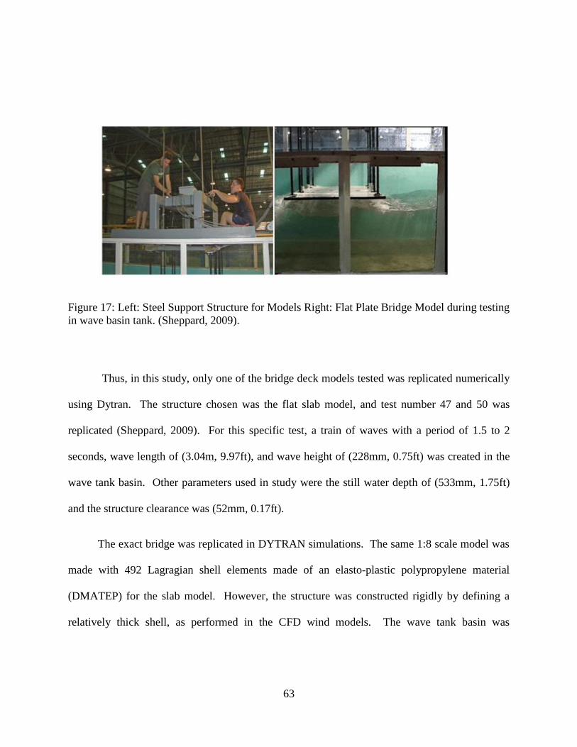
63
Figure 17: Left: Steel Support Structure for Models Right: Flat Plate Bridge Model during testing
in wave basin tank. (Sheppard, 2009).
Thus, in this study, only one of the bridge deck models tested was replicated numerically
using Dytran. The structure chosen was the flat slab model, and test number 47 and 50 was
replicated (Sheppard, 2009). For this specific test, a train of waves with a period of 1.5 to 2
seconds, wave length of (3.04m, 9.97ft), and wave height of (228mm, 0.75ft) was created in the
wave tank basin. Other parameters used in study were the still water depth of (533mm, 1.75ft)
and the structure clearance was (52mm, 0.17ft).
The exact bridge was replicated in DYTRAN simulations. The same 1:8 scale model was
made with 492 Lagragian shell elements made of an elasto-plastic polypropylene material
(DMATEP) for the slab model. However, the structure was constructed rigidly by defining a
relatively thick shell, as performed in the CFD wind models. The wave tank basin was

64
constructed with over 77,000 Eulerian Quadrilateral Solid Elements (CHEXA). Figure 18 shows
both the Eulerian and Lagragian Mesh of the CFD model used for wave tank verification.
In Dytran, all of the geometric quantities were modeled exactly and the wave was not
created but rather initialized with the corresponding parameters discussed above. Therefore the
only assumption required in the program was the velocity at which the water is translating
forward. No information is provided about this from the report and therefore a reasonable
assumption of (0.5-1 m/s, 1.64-3.28 fps) was assumed for the numerical models based on the
wave period and estimated wave width.
Figure 18: CFD model from DYTRAN of UF wave tank experiment. Top: Blue: Eulerian
Elements (Fluid) White: Lagragian Elements (Structure). Bottom: Input shape of Setup Wave for
Test Number 50. Input Wave Velocity in Positive X-Axis
65
To ensure that all effects of the wave loads are seen in the CFD models, a comparison
was conducted on the time dependent load cell readings. In DYTRAN, several nodes were
selected and a time varying force was recorded. This allowed for direct comparison of the
maximum and minimum vertical forces and the power spectral density (PSD) of the signal.
Additionally the load rise time tr was observed for each event which is a determining parameter
for classification of the loading as quasi-static or slamming.
Prototype Structures and Location
Performance based engineering is typically performed for a specific structure in a
specified location. In this study the region of interest will be the Tampa Bay/Sarasota area. This
area of the State of Florida is host to numerous coastal structures, including the Sunshine
Skyway Bridge, MacDill Air Force Base, and numerous shoreline hotel structures that are
typically 8-15 stories tall. Tampa Bay, has been spared from a major hurricane since 1921 in
which a 100+ mph Hurricane made landfall at Tarpon Springs, causing six deaths. However,
during that time Tampa Bay had a population of 135,000 and today more than 2.5 million people
reside in the area. Additionally the bathymetry of the Tampa Bay Area is very conducive to
excessive storm surge, which makes it vulnerable to large hurricanes. All of these factors
decrease the expected performance of the empirical design based structures in the region.
Therefore, results from structures in this region may substantiate the need for refinement in the
current structural engineering field.

66
Building Model
The prototype building used in this study was obtained from a Reinforced Concrete
Design Handbook. The building consists of a three story one way joist and slab system with
typical bay spacing of (9.1mX9.1m, 30‘X30‘). Each story is thirteen feet tall and the total plan
dimensions of the structure are (27.5mX45.7m, 90‘X150‘). The building was designed with no
shear walls and uses the beam and column framing as the lateral restraint system. The building
was designed in a very high wind prone region, with 145mph as the design wind speed. This
design wind speed is slightly higher than the base wind speed in the Tampa-Bay region,
according to ASC 7-02 which is approximately (58-60m/s, 135-130 mph). The structure was
designed for typical Dead Load (DL) and Live Load (LL) of (6.22kPa, 130psf) and (2.87kPa,
60psf), respectively, that is typically found in an office building or hotel.
Using this load data, the structure was designed per American Concrete Institute (ACI)
code and all reinforcing steel was sized for the columns and beams. The columns and beams
were reinforced with a 5% and 3% steel percentage respectively. The concrete and steel
reinforcing grades chosen were (27MPa, 4000psi) and (420MPa, 60,000psi) respectively due to
their common use in the design industry.

67
Figure 19: Plan and Elevation view of Prototype Building used in Study for Wind Tunnel and
Wave Tank Testing
Bridge Model
The bridge model chosen for this study was based on the Anna Marie Island Bridge
replacement project currently under consideration since 2008. The existing bridge consists of
several concrete beam fixed span segments and a bascule type span in the main channel
approximately (5.3m, 17.5ft) above the mean water high. The bridge connects the Anna Marie
Island to the mainland near Bradenton, Florida, as seen in Figure 20. During the Project
Development and Environment (PD&E) study, wind tunnel testing was carried out on several
different bridge deck configurations on a 1:60 scale ratio at the RWDI Miramar, Fl BLWT.
Therefore this bridge was chosen due to the availability of data from wind tunnel testing and its
applicability of a typical coastal bridge.

68
Figure 20: Left: Existing Anna Marie Island Bridge. Right: View of Anna Marie Island in Tampa
Bay and Study Bridge Location (Mara & King, 2008)
The wind tunnel testing carried out at the BLWT facility was conducted on two different
bridge deck geometries. These bridge deck cross sections can be seen in Figure 21. For this
study the smaller cross section was chosen, with 6 girders for modeling and analysis.
Measurements from the BLWT from a hotwire anemometer provided information on the mean
wind speed and turbulence intensity for various elevations for the bridge deck placement.
Additionally, smoke flow visualizations were conducted to see the effect of the barrier placement
on the wind vortices that developed. These results will be used a validation tool for the CFD
models implemented in this study.

69
Figure 21: Section Views of Anna Marie Island Bridge Deck Alternatives (Mara & King, 2008)
Since the full design of the bridge has yet to be determined, a typical Florida Pre-stressed
T-78‖ bulb beam was chosen for the main girders of the bridge deck. A Florida T-78‖ Beam was
chosen due to its large span applicability (typically around (36.5m, 120ft)) and predominant use
in Florida bridges. Additionally, the new bridge deck height has yet to be determined and
therefore the existing deck height will be used for this analysis.
To simplify the structure for use in the wind tunnel and wave tank for software reasons,
the depth change between the slab and girder was not modeled and the flanges of the beams were
connected continuously, to create a smooth undersurface to the deck. The bridge model was
created out of 242 Shell elements and was comprised of over 8938 quadrilateral elements
(CQUAD). The properties of the shells were defined from standard concrete values used in

70
design. The model was constructed rigidly by defining the thickness of the shells to be large, in
comparison to the dimensions. A picture of the bridge model is shown in Figure 22.
Figure 22: Bridge Model Used in Wind Tunnel and Wave Tank CFD simulations
Probability Distribution Analysis
Once a specific locations and structure of interest has been determined, the first step in
hazard analysis in a Performance Based Design is to statistically define the magnitude and
probability of occurrence of these hazards occurring both individually and simultaneously.
Probability Distribution Analysis is a vital step in applying PBE. Since the performance of the
structure is related the hazards associated with it, then full probabilistic quantities are required to
map structural response/damage to category of hurricane. This step in PBHE is currently quite

71
well understood and can be thoroughly explained in Simiu and Phan et al. (2007). However the
existence of structure specific dynamic data from hurricane hazards is currently non-existent.
Statistical information from the Tampa Bay region was collected from annual records and
computer simulations through NOAA and NIST. The statistical data was not collected from
actual hurricane conditions, and would only be used for identifying statistical quantities, such as
the return period for damage assessment. Each hazard was then described by an appropriate
probability distribution function for the given location. Once each hazard‘s marginal distribution
has been defined, a joint probability distribution can be determined with additional knowledge of
the correlation between the hazards. These results will then be combined with the dynamic time
history data generated to allow for scaling of the record to any particular event.
Prototype Dynamic Time History Generation
Once the accuracy of CFD modeling were confirmed through the verification studies the
generation of Dynamic Wind and Wave time history data was the main subject of this study.
CFD model simulations were carried out on the MSC Dytran platform. These results were then
standardized into pressure and force coefficients. This process will enable a spectrum of loads
corresponding to each storm category to be created and applied to later structural models.
Extreme Winds

72
First, annual extreme non-directional wind speeds were collected from NIST for the
Tamp Bay region from 1951-1990. A 10m corrected 3-second annual extreme wind gust was
reported. This data was collected for insight into the historical wind records available.
Next, dynamic data was created using CFD wind tunnel simulations of the building and
bridge under consideration. Both structures were placed in the Dytran Fluid Solver to develop
time history records of wind pressure on various sections of the models as shown in Figure 23
and Figure 24. From each time history record, the forces/pressures can be converted to pressure
coefficient as typically done in wind tunnel testing. From this non-dimensional coefficient, a
time history of pressure can be obtained for each storm category by scaling the pressures by the
appropriate expected mean wind speed.
Figure 23: Building Model in Wind Tunnel CFD simulation. Flow in the positive x-direction.

73
Figure 24: Top: Bridge Model in Wind Tunnel CFD simulation. Flow in the positive x-direction.
Bottom: Location of Pressure/Force Readings taken during simulation.
Surge Height
For the present study, SLOSH generated storm surge data was utilized for analysis. The
Tampa Bay basin was used and the corresponding SLOSH grid for the basin is shown in Figure
25. The SLOSH program employs a telescoping polar grid coordinate system within each coastal
basin. As a result, good resolution data is provided for areas of interest along the coast and inlet
bays, while conserving computer resources.
The SLOSH Grid for the Tampa Bay Region consists of approximately 58 radial and
curved lines, making up approximately 3100 regions. Each grid region covers approximately 1.5
square miles. The SLOSH model requires only the category of the hurricane, direction of wind

74
speed and landfall tidal condition (high, medium, low) for calculation of anticipated storm surge
heights. All possible surge conditions were recorded for the prototype building and Anna Marie
Island Bridge.
Figure 25: Tampa Bay region SLOSH Grid
Time dependent surge heights were generated not in this study and rather it is suggested
that it should be treated as a static load. Storm surge is typically relatively constant for the study
location, and the only fluctuation in the height is due to the astronomic tidal heights. Therefore
the expected storm surge can be drastically different if the storm is expected to make landfall
during high, low or normal tide conditions. Therefore, taking a look at the astronomic tidal
variation in the Tampa Bay region was conducted using SLOSH and shown in Figure 26. As

75
you can see from the Figure, the fluctuation in tidal height is relatively constant over a 1-2 hour
window, which is the expected extreme loading duration of the hurricane event for a structure.
The change in astronomic tides is very small and typically around (30-60mm, 0.1-0.2ft) during
this window.
Figure 26: Astronomic Tidal Predictions for Tampa Bay region from SLOSH
Wave Simulations
Similar to the extreme wind speed hazard, both annual extreme wave data was collected
and numerical modeling of wave loads was conducted. First significant wave heights were
collected from NOAA buoy number 42099 located in the St. Petersburg area as shown in Figure
27 for a three year period. The significant wave height is calculated by averaging the top 1/3 of

76
the entire wave heights recorded during a 20 minute interval. The wave height intensity data
was appropriately described by the log-normal distribution.
Figure 27: Picture and Location of NOAA Wave Buoy Number 42099
Next, dynamic data was created using CFD wave tank simulations of the building and
bridge. A single wave height and period was modeled and measured forces were converted into
a non-dimensional force coefficient. This was performed by scaling the load by the water
density (ρw), acceleration of gravity (g), significant wave height (Hs), and tributary area (A).
Then estimates of the anticipated wave forces for each category of hurricane dynamic wave
forces can be developed for each model by scaling the appropriate non-dimensional force
coefficient.
However, the full dimensions of the building were not modeled in a wave tank but, rather
a square shape representing the column will be modeled This approach was taken due to the

77
high likelihood of building envelope failure and loss of the curtain wall for the first story with
the presence of wave action. Therefore, only the primary structural members, such as the
columns, would be subjected to wave forces for the first story. This assumption was also used
for all of the wind loading calculations for the building.
Finite Element Structural Models
Once Dynamic Loads were generated for both prototype structures, a detailed FEM was
created for linear structural analysis. To simplify the structural analysis process due to time
constraints, a 2-D model of a frame was constructed of the three story building and a single span
of the Anna Marie Island replacement bridge was modeled. Each model was created in SAP to
full scale, utilizing frame and shell elements. A short description of each model is given below
followed by a figure of each model.
The 2-D building model was constructed entirely of frame elements, which were given
their respective cross section dimensions and reinforcement properties previously determined
from ASCE 7-05 wind design procedures. Fixed support conditions were enforced along the
base of the structure. Wind Loads were applied at floor locations where the building‘s facade or
curtain wall would be attached to the main structural framing. Wave loads were applied at each
node, from the base of the columns of the structure to their respective wave crest plus surge
height.
The Bridge Deck model was constructed of both frame and shell elements. Frame
sections were modeled for each girder and were given AASHTO Beam Type VI properties (72‖).
A (250mm, 10‖) reinforced concrete deck shell was then modeled (0.9m, 36‖) above the frame

78
elements which were then rigidly linked together. The (30.5m, 10ft) long by (18.3m, 60 ft) wide
bridge deck was coarsely meshed into (0.3m, 1 ft) lengths to enable easy application of nodal
time histories. Pin support boundary conditions were enforced on the ends of the each frame
element end where each span would rests on the pier caps. Additionally, the crash barrier was
not modeled in the structural model, but its tributary was taken into account when applying the
loads. Wind loads were placed on the structure on several nodes and wave loads were applied to
the barrier and the bottom of the bridge deck.
Figure 28: Building Model in SAP

79
Figure 29: Bridge Model In SAP
Load Cases
Only a select number of realizations of the wind and wave hazard were investigated. For
this study wind speeds for hurricane categories I-V corresponding to [33 40 49 58 67m/s, 75 90
110 130 150mph] and significant wave heights from [0.6 0.9 1.2 1.5 1.8m, 2 3 4 5 6ft] were used
for structural evaluation. The resulting storm surge from each storm category was then
determined from SLOSH. Each hazard was applied to the structure in separate and combined
cases to see their individual and collective effects. Structural demand parameters such internal
bending moment and shear were plotted against the two dynamic hazards in this study.
80
CHAPTER FOUR: RESULTS
Wind Tunnel Verification
A comparison of the four faces of the model is shown below in Table 1. Results are shown
for both wind attack angles of 45 and 15 degrees from the longitudinal axis of the building.
The Dytran signal and wind tunnel mean pressure coefficients agree well. All five faces of the
structure have mean pressure coefficients in agreement on the order of 5%. This result agrees
with other researchers such as Dagnew et al. (2009) and Holmes et al. (2001) in, that accurate
static mean pressures can be achieved through numerical wind tunnel modeling techniques.
However, a more scientifically precise description of the loading is required for PBE and
therefore dynamic characteristics of the signal are vital.
The frequency content of the signal was investigated next using the PSD. An example of a
comparison of the PSD of the various methods described is shown in Figure 31, for the
windward wall. PSD comparisons for all five locations are included in the Appendix. From the
PSD comparisons, a very good agreement is seen between the wind tunnel and Dytran
simulation. No difference is seen in the magnitude of the power of each signal, but a small
horizontal shift is seen in the frequency axis occurs due to normalization of the PSD. If no
normalization is used on the horizontal axis, these two curves align. Additionally, the
established wind spectrum equations approximated the two methods accurately. Some minor
differences are seen in the higher frequency range between the predicted spectrum and the two
modeling techniques. This pattern was seen in all of the PSD comparisons, which can be found
in the Appendix. This result may be attributed to high sampling frequency use for the

81
experiment. A desirable upper limit is 200Hz (Holmes, 2001), which was used for down-
sampling.
Figure 30: Location of Signal Comparisons on Barn Structure
Table 1: Mean Pressure Coefficient Comparison
Structure
Location
Mean Pressure
Coefficient
Wind Tunnel
Mean Pressure
Coefficient
DYTRAN
ASCE 7-05
Analytical
Procedure
WIND
ATTACK
(°)
45 15 45 15 -
Windward
Wall
0.22 0.56 0.19 0.54 0.40
Windward
Roof
-0.27 -0.45 -0.32 -0.50 -0.69
Roof
Peak
0.32 0.53 0.35 0.49 -
Leeward
Roof
-0.19 -0.27 -0.15 -0.22 -0.37
Leeward
Wall
-0.37 -0.21 -0.30 -0.20 -0.29

Figure 31: PSD Comparison of Wind-Ward Roof

An example of an autocorrelation function comparison is shown in Figure 32. In the Figure,
the windward roof autocorrelation functions of the two modeling methods are compared. Only
minor differences are seen in the magnitude and the shapes are identical. Again, all of the
comparisons are provided in the appendix.
Figure 32: Autocorrelation Function Comparison of Windward Roof Pressure
A comparison of the integral length scale of the various faces of the structures is shown
below in Table 2. The agreement between the two is not as accurate as the previous parameters
compared. This deviation give rise to the horizontal scale shift of the PSD plots discussed

84
earlier. One reason for this discrepancy may be due to the fact that the longitudinal turbulence
fluctuation is based on the frictional velocity (u*), which is further derived from the surface
roughness of the wind record. The surface roughness is not a definitive quantity and was merely
estimated from dimensions of roughness elements, using a primitive method that has been
updated very little in the last 30 years. Additionally, the surface roughness in the wind tunnel
models could not be replicated in the numerical simulations, due to the tremendous
computational demands it would require.
Table 2: Integral Length Scale Comparison
Structure
Location
Integral Length
Scale Wind
Tunnel (m)
Integral
Length Scale
DYTRAN
(m)
WIND
ATTACK
(°)
45 15 45 15
Windward
Wall
.040 .086 .087 .293
Windward
Roof
.033 .017 .063 .024
Roof
Peak
.026 .043 .014 .025
Leeward
Roof
.023 .020 .098 .017
Leeward
Wall
.035 .012 .012 .014
The values of the turbulence intensity for the two different models, as well as the
predicted intensity given in Equation 5, are shown in Table 3. The comparison shows that
Dytran is consistently measuring lower turbulence intensity values than the wind tunnel models.
This finding suggests that fluctuating pressures are not being accurately captured in the Dytran

85
simulation. A source of the discrepancy may be due to the fact that no randomness of the
velocity profile is input into Dytran, and only a constant velocity profile is allowed. Therefore
the lack of turbulence is attributed to the limited number of roughness elements use to develop
vortices. Also, the turbulence intensity predicted by Equation 8 is appreciably different than
both sets of collected data. Equation 8 was based on measurements produced by large scale
depression systems (Holmes, 2001). Therefore it is not entirely applicable for BLWT modeling
conditions.
Table 3: Longitudinal Turbulence Intensity Comparison
Structure
Location
Longitudinal
Turbulence
Wind Tunnel
(%)
Longitudinal
Turbulence
DYTRAN
(%)
Longitudinal
Turbulence
Equation 8
(%)
WIND
ATTACK
(°)
45 15 45 15 45 15
Windward
Wall
12.3 31.8 4.6 19.4 46.5
Windward
Roof
15.6 25.6 8.6 13.4 49.6
Roof
Peak
18.1 29.8 9.8 15.6 58.9
Leeward
Roof
10.5 15.3 8.3 7.9 49.6
Leeward
Wall
21.0 11.7 5.1 10.1 46.5
Next, comparisons of the SDOF oscillator are shown in Figure 33. The response of the
two systems is quite different. Consistent with the turbulence intensity measures, the Dytran
response reaches a steady state after several seconds of duration and that is not seen in the wind
tunnel. The initial responses of the two methods are merely identical, and differ in magnitude by

86
5-10%. After approximately one second of loading the Dytran system has reached a constant
position and exhibits relatively no dynamic response. The wind tunnel SDOF oscillator
continues to display dynamic movement for the entire loading duration of ten seconds.
Figure 33: SDOF Comparisons for Wind Wall. Left: Dytran. Right: Wind Tunnel
DYTRAN WIND TUNNEL
0 5 10 151 10
5
0
1 105
Veloci ty
v1
m s1
t
0 5 10 154 10
4
2 104
0
2 104
4 104
6 104
Acceleration
a1
m s2
t

87
From these results, an investigation was performed on the Eulerian mesh to ascertain why
Dytran results approach steady state after such a short duration. Figure 34 shows the
development of the air vortices over time as the program is running. The velocity profile over
the building is relatively constant after the initial front. The flow of the air over the structure is
limited to streamlines of constant velocity and relatively no mixing or creating of eddies are
visible after the initial front. Additionally vortex shedding in the wake of the building is the only
source of turbulence seen in the mesh. This phenomenon occurs regardless of the turbulence of
the upstream flow and is simply related to the Strouhal number (Holmes, 2001).
Therefore, from these results the Eulerian mesh was inspected to give hints as to why the
Dytran results reach such a steady state. Therefore, it is believed that these vortices that are
created in the experimental wind tunnel are created due to the non-ideal creation of the wind
flow. Typically, wind tunnels are constructed with a series of large fans or blower systems that
create the flow striking the structure over a long roughness surface. The roughness elements used
in the numerical simulation were limited and the true wind tunnel testing has a series of over 25-
30 rows of these elements. These additional elements may help create the additional vortices
that are lacking in the numerical simulations. However, the addition of more roughness elements
is not feasible in this study due to the increased simulation runtime. To combat this issue, the
idea of random pulse generation (RPG) was investigated.
Random pulse generation is typically performed in seismic research to create synthetic time
dependent ground motion and has been shown to be a very versatile tool for simulating a large
class of physical phenomena (Lin and Cai, 1995). The signal is considered to be composed of a
series of

88
Figure 34: Development of Wind Turbulence (eddies) in Eulerian Mesh of Barn Wind Tunnel
Study. Velocity of Wind (m/s) is shown in Contours

89
pulse trains, which are a repetitive series of random magnitude pulses (Yj) that are separated in
time by a random arrival time (τj). If a linear assumption is valid for the combination of the
pulses and each random pulse magnitude (Yj) is independent of the arrival time, then a series of
(N) pulses can be combined to obtain the signals evolutionary spectral representation (X). This
result allows for synthetic generation of a random seismic signal in the frequency domain from a
series of single pulses as shown in Equation 9. Where w(t-τ) is a deterministic pulse shape
function satisfying the condition w(t,τ)=0 for t>τ (Lin and Cai, 1995).
(9)
However, the Navier Stokes equations are a set of non-linear second order differential equations
and therefore the direction superposition of signals arriving at each timeframe will not recreate a
signal with 100% accuracy. However, it will allow for turbulence to be introduced into the
signals. Therefore, it was conceivable that the combination of several simulations of the same
structure under different obstacle placements would allow random pulse generation to be applied
to the signals. Numerous simulations would be required to produce enough data to generate a full
10 second record. To accomplish this, ten computers were simultaneously programmed to run
various placements of barriers on the barn structure. Random pulse generation was then applied
to the various data sets to create a suitable final signal.
For random pulse generation, the most important quantity needed for a synthetic signal
generation is the time/source relationship. Through this relationship, the time/delay between
)(
1
)()(TN
j
jj twYtX

90
successive arrivals of signals is used to create the final signal. For this study, the time/delay of
the arrival of wind vortices was calculated from the speed of the wind and the upwind distance.
This time was found to be about 0.25 seconds and corresponds to approximately 50-100 samples
depending, on the velocity of the wind. Additionally, due to the fact that the measured pressures
oscillate about a mean instead of zero, the mean value of the entire signal was subtracted when
two signals were added together. Using this idea, a synthetic signal was constructed with a
varying arrival rate of successive signals.
Comparisons were then recomputed for the mean pressure coefficient, autocorrelation
and PSD to ensure that the signal was not significantly altered using this technique and only the
turbulence component is affected. All of these results are shown in the Appendix with the
subtitle RPG. The dynamic response does not reach a steady state and the numerical values are
very comparable to the wind tunnel response for the entire length of the record. The frequency
content of the displacement response was compared with a FFT based PSD.

91
Figure 35 PSD comparison of Displacement Response of SDOF
Figure 35 shows that the RPG addition to the Dytran signal shifted the shape of the PSD
plot in line with the wind tunnel response. The original raw dytran signal had a significant
amount of higher frequency response. From these results, it was concluded that the CFD
technique could be combined with RPG to create a suitable dynamic signal without adverse

92
affects on the frequency content of the signal as shown in the PSD plots. In all three signals a
distinct peak is seen around 0.2Hz which is less than the natural frequency of the barn of 5Hz.
Wave Tank Verification
To ensure that the wave loading phenomenon is accurately captured, both the time and
frequency domain content were examined. First, the signal was passed through a Chebyshev
low-pass filter which was used to remove the excessive high frequency content obtained in the
raw signal. Chebyshev Filters have a steep roll-off but, have more passband ripples than
Butterworth filters (Daniels, 1974). A cutoff frequency of 25Hz was used as to not induce
excessive extension of the loading time history. Once completed, the maximum and minimum
loads recorded from the experiment and numerical simulations were compared for both the
horizontal and vertical directions. A typical comparison of the two methods is shown in Figure
36 and Figure 37.
Dytran captures additional high frequency slamming forces that are associated with
waves. The quasi-static varying load is also not as apparent in the numerical simulations, but is
quite similar to slamming force shown in the experimental study. The recorded peak load is
approximately (325N, 73lbf). This value is quite comparable to the records from Sheppard, in
which a maximum slamming force of (333N, 75lbf) was recorded for Test #50 (Sheppard, 2009).
This was also representative of the horizontal load comparison as a (8N, 0.48lbf) difference
(approximately 10%) was measured. A summary of the vertical and horizontal load comparisons
can be found in Table 4. The variation was not of a great concern, due to the large deviations in

93
both magnitude and shape of wave time histories reported for similar test conditions by
numerous laboratory basin studies (Cuomo, 2007).
Table 4: Force Comparisons for Wave Tank Modeling
Test #47 Test #50
Dytran Experiment Dytran Experiment
(lbf) (lbf)
Vertical 72.8 60.06 73.06 75.07
Horizontal 1.8 2.23 3.60 4.08
Once the maximum and minimum peak loads were compared, each force time history
was converted into a non-dimensional time history. Each time history was normalized by the
density of water, acceleration of gravity, tributary area, and significant wave height. This
process will enable the recreation of simulated peak pressures for any wave height, and further
comparison against other researchers such as Cuomo et al. 2007. These plots are shown in the
appendix under Bridge Wave tank verification. For the two test simulations, the vertical peak
pressure was found to follow the empirical relationship given in Equation 10. This result is quite
comparable to other peak vertical forces in which the range of (1.8-7.6) is given. However, more
simulations are required to give a definite empirical relationship.
(10)
swv gHP )25.1(

94
For the frequency domain comparison the power spectral density computed using two
methods is compared, as shown in Figure 38 and Figure 39, the numerical simulation shows a
much higher frequency loading distribution than the wave basin studies. This high frequency
loading is not typically found in natural wave phenomena, as shown from a PSD plot from the
wave buoy data collected (Figure 40). Wave buoy data doesn‘t suggest any wave frequencies
above the 0.5 Hz range. However, this data was not collected from impact studies, and is a
measure of the natural wave cyclic frequency.
Figure 36: Vertical Time History from Flat Slab Structure Test (Sheppard, 2009)

95
Figure 37: Vertical Time History From Dytran Simulation
Figure 38: PSD Plot From Wave Basin Study on Vertical Load Cell (Sheppard, 2009)
.

96
Figure 39: PSD Plot of Dytran Time History Force
Figure 40: PSD Plot from Wave Buoy 42099 (NOAA)

97
After a thorough examination of these verification studies, it was concluded that an
accurate quantification of the wind and wave hazard can be performed with CFD numerical
simulations. Although slight differences are seen in the time and frequency content of the signal
provided by the numerical approach, the margin of error of 5-10% is considered acceptable.
The CFD simulation approach is then extended to study the hurricane hazards for two structural
systems typically found in the State of Florida.
Probability Distribution Analysis
Probability Distribution Analysis was carried out for all of the hazards included in this
study. First, an appropriate distribution fit to a measure describing the intensity of each hazard
and then joint probability analysis was carried out. The correlation between the various hazards
was assumed in this study and the Nataf method for joining correlated multivariate distributions
was utilized, as described in Der Kiureghian et al. (1986).
For the extreme wind speed records gathered the Gumbel/Type I Largest Distribution was
found to fit the data accurately. Gumbel (1954) introduced the methodology for fitting recorded
annual maxmima events, which has been typically applied to flood prediction and extreme wind
speeds (Holmes, 2001). The parameters of the distribution, along with a plot of the fit is shown
in Figure 41. The return period for wind speeds (31m/s, 70mph), (40m/s, 90mph) and (49m/s,
110mph) is 8, 80 and 250 years respectively.

98
Figure 41: Gumbel Distribution fitting to Extreme Wind Speed from Tampa Bay (1951-1990)
For the surge height data collected from SLOSH, the exact coordinates of the structures
location was extracted for all storm levels, forward directions and tidal conditions resulting in
over 200 combinations. An example of the significant storm surge expected in the Tampa Bay
region is graphically shown in Figure 42.
FIT PARAMETERS
β=0.116
α=52.8

99
Figure 42: SLOSH Surge Height Results from Category I at mean tide on Left and Category IV
at mean tide on Right.
Once the data was extracted, the generalized extreme value distribution accurately fit the
Tampa Bay surge data, as shown in Figure 43. However, this approximate distribution is only
valid for the specific location of the structures, as surge heights in the the next grid basin may be
drastically different.
Significant wave heights in the Tampa Bay region were accurately described by the
lognormal distribution, as shown in Figure 44. However, this data was collected from an
offshore buoy and the expected wave height that may reach the inland structures, such as the
building under consideration, is significantly reduced. According to Wu et al. (2006) due to
wave decay once reaching shore, the typical wave height that reaches an inland structure is only
10-20%.

100
Figure 43: Extreme Value Probability Density Function Fits to Surge Data
Figure 44: Log Normal Probability Density Function Fit To Significant Wave Height Buoy Data
from Station 42099 (2007-2009)
Once each hazard has described by an appropriate density function, a joint probability
analysis was carried out. For this analysis, the correlation coefficient between wind and wave
hazards and wind and storm surge was assumed to be 0.5. This is a relatively strong correlation
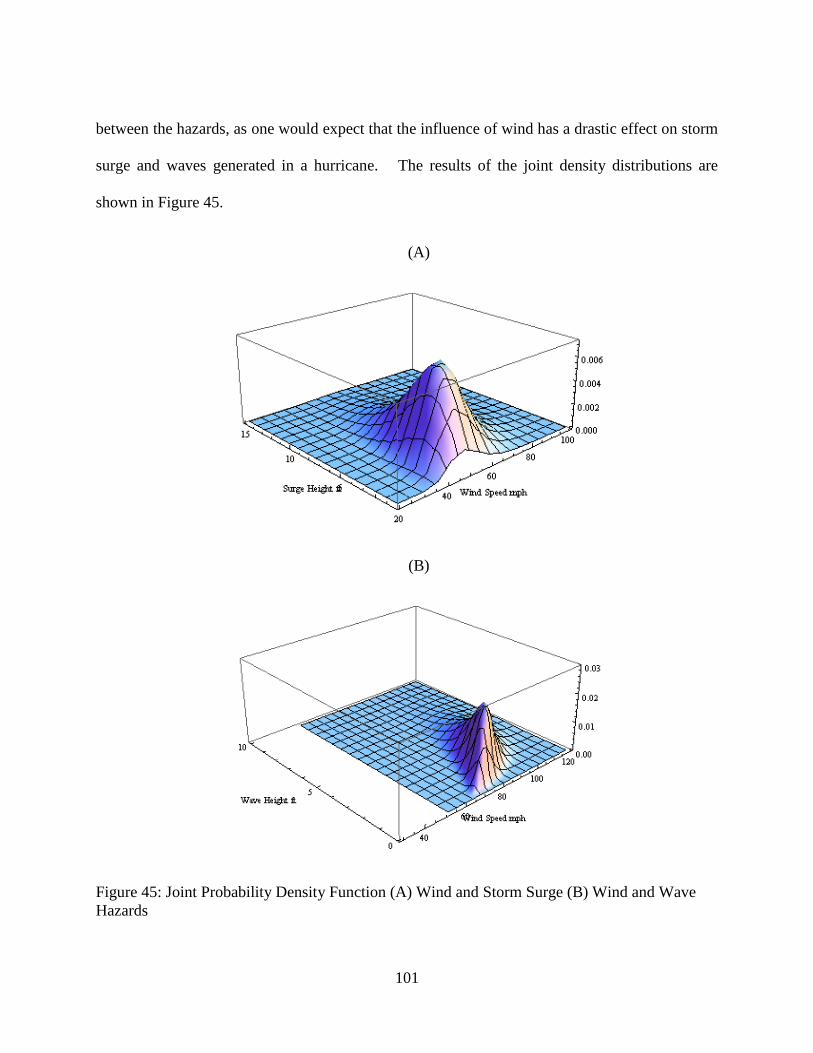
101
between the hazards, as one would expect that the influence of wind has a drastic effect on storm
surge and waves generated in a hurricane. The results of the joint density distributions are
shown in Figure 45.
(A)
(B)
Figure 45: Joint Probability Density Function (A) Wind and Storm Surge (B) Wind and Wave
Hazards
102
Dynamic Wind and Wave Load Generation
Dynamic wind loads were generated for both prototype structures considered in this
study. Therefore, no experimental or full scale pressure coefficients were available for
comparison. The sampling frequency and the input velocity were the only parameters changed
from verification models. Each parameter was set as 200Hz. and (12m/s, 39fps), respectively.
Only one angle of attack was used to create the time history data, due to high computational
demands of each simulation.
The data was then assembled through RPG into a suitable 25 second signal which was
then analyzed in both the time and frequency domain. Nodal time histories were converted into
a non-dimensional pressure coefficient for application to each FEM. An example result is shown
in Figure 46 and Figure 47 for the second floor windward wall of the building model. Results
correlated well with previous verification studies as the pressure coefficient varies around 0.50.
The wind PSD plot aligns with the established design code spectrum and only a slight shift is
seen in the frequency domain due to the normalizing terms. These findings were typical for all
locations recorded for the building and several more results are provided in the Appendix.

103
Figure 46: Second Floor Time History Windward Wall
Figure 47: Second Floor Windward Wall PSD Comparison

104
Dynamic wave loads were also generated for both the bridge and building in this study.
Scaled models were placed in the numerical wave tank, and a particular wave height and period
impacted each structure. Horizontal and vertical forces were then sampled at 200Hz and passed
through the Chebyshev Type I lowpass filter. Similar to the wind loads, a non-dimensional force
coefficient was created and sample results are shown in the appendix. Additionally the wave
time histories were visually inspected for the number of the slamming pulses. Various studies
such as Sheppard et al. (2009) indicate that the number of slamming pulses is directly related to
the number of air chambers. Figure 48 and Figure 49 show that Dytran is accurately reproducing
5 distinct slamming pulses for the six girder bridge.
Figure 48: Dytran Vertical Time History for 5 Chamber Bridge
0 0.1 0.2 0.3 0.4 0.5 0.6 0.7 0.8 0.9 1-0.2
0
0.2
0.4
0.6
0.8
1
1.2
1.4Vertical Pressure Time History
Time, sec
Norm
alized V
ert
ical P
ressure
, P
/pgH
s

105
Figure 49: Girder Spacing Effects on Wave Forces (Sheppard, 2009)
Dimensional Scaling
Before application of the dynamic loads to each FEM, scaling effects due to Froude and
Reynolds number modeling were considered for the wave and wind hazards respectively. Due to
prototype and model scaling ratios both the time and magnitude of the loading signal must be
performed.
For wind tunnel modeling a total of sixteen dimensional quantities such as the mean wind
speed (u), roughness length (zo), and density of air (ρa) must can be described in thirteen
dimensionless quantities such as the Jensen number and Reynolds number (Holmes, 2001). For
accurate modeling of the wind effects between model and prototype structures these
dimensionless quantities should be equivalent. Due to these effects, results from the wind tunnel
must be modified in the frequency domain due to the reduced frequencies at model scale and at

106
prototype scale as shown in Equation 11 (Main and Fritz, 2006). Where the model-scale
frequency (fm), model wind speed (Vm) and length scale (λL) are fixed due to wind tunnel
modeling conditions, and the prototype sampling frequency (fp) is proportional to the desired
prototype wind speed (Vp).
(11)
For wave tank modeling dimensionless quantities such as the Mach number, Weber
number, Froude Number and Reynolds model can be chosen to obey similitude laws.
Historically the Froude number has been used exclusively for scaling ratio used for offshore
structures and ship testing (Cuomo, 2010). Therefore using this similitude law scaling factors for
the measured pressures and forces are shown in Table 5.
Table 5: Froude Scaling Laws
Froude Scaling
Length λ
Mass λ3
Force λ3
Time 𝜆
However from a comparison of laboratory and full scale pressures by Allsop et al. (1996)
suggested that Froude scaling overestimates measured wave loads by 92-99%. Froude scaling
L
m
p
mV
Vf
pf
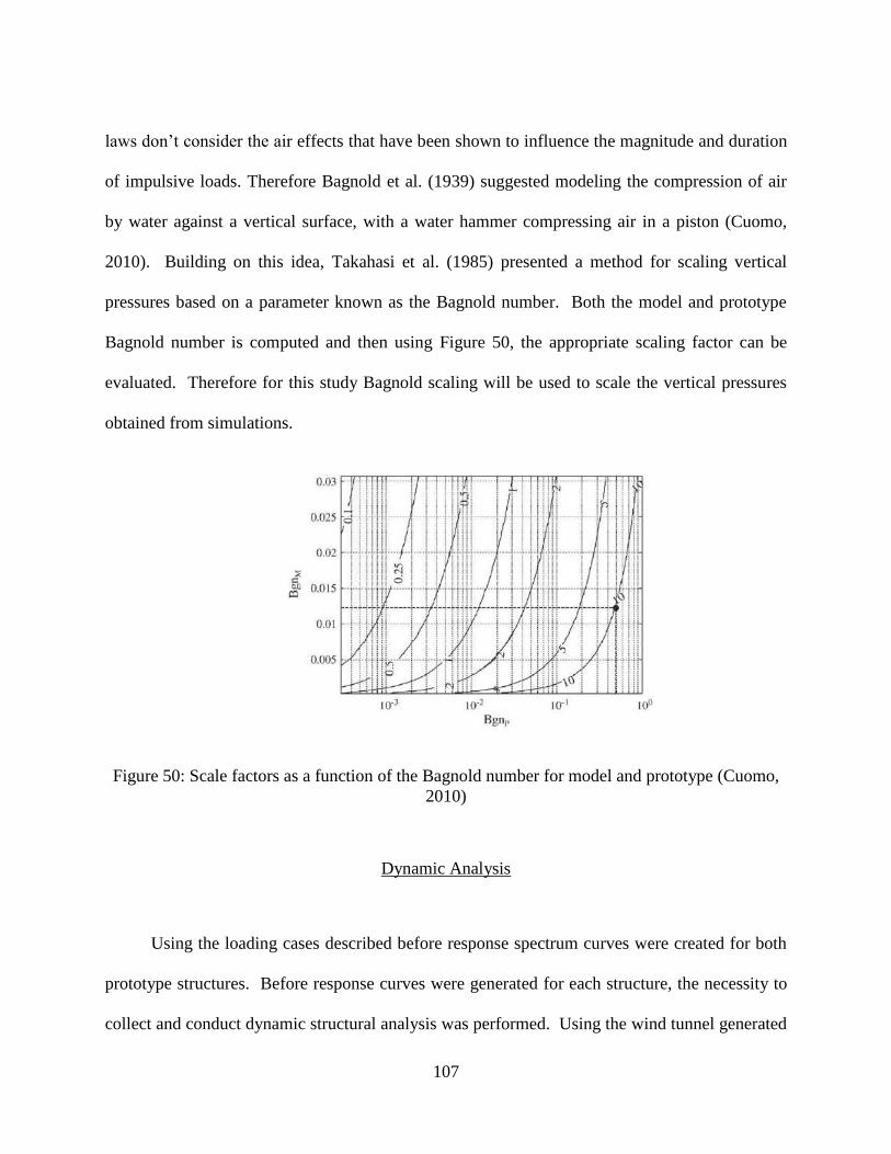
107
laws don‘t consider the air effects that have been shown to influence the magnitude and duration
of impulsive loads. Therefore Bagnold et al. (1939) suggested modeling the compression of air
by water against a vertical surface, with a water hammer compressing air in a piston (Cuomo,
2010). Building on this idea, Takahasi et al. (1985) presented a method for scaling vertical
pressures based on a parameter known as the Bagnold number. Both the model and prototype
Bagnold number is computed and then using Figure 50, the appropriate scaling factor can be
evaluated. Therefore for this study Bagnold scaling will be used to scale the vertical pressures
obtained from simulations.
Figure 50: Scale factors as a function of the Bagnold number for model and prototype (Cuomo,
2010)
Dynamic Analysis
Using the loading cases described before response spectrum curves were created for both
prototype structures. Before response curves were generated for each structure, the necessity to
collect and conduct dynamic structural analysis was performed. Using the wind tunnel generated

108
dynamic time history data the frequency was scaled and corrected according to the reduced
sampling frequencies at model scale. This data was then transformed into the frequency domain
to obtain the dominant forcing function frequency. This value was found to be approximately
0.5Hz. Then the reduced sampling frequency was reduced further to obtain dominant wind
frequencies of 0.1Hz, 0.08Hz and 0.03Hz. All of these forcing functions were then applied at the
same wind speed to the building model and third floor response was recorded. These plots were
then simultaneously plotted in Figure 51.
Figure 51: Dynamic Amplification of top floor displacement with dominant wind Frequency (F)
DAF
1.6

109
From the figure a clear dynamic amplification factor can be seen. The response is
approximately 1.6 times the lowest dominant wind frequency which is approximately static.
This result confirmed the need to consider the dynamic effects of the hurricane hazards
Next, response curves for the building and bridge were created for all loading cases
considered. Results for the building can be found in Figure 52 and Figure 53 and results for the
bridge can be found in Figure 54 and Figure 55.
Figure 52: Drift Index Response Curve

110
Figure 53: Ratio of Ultimate Moment Strength for First Floor
Figure 54: Bridge Horizontal Displacement Response Curve

111
Figure 55: Bridge Midspan Moment Response Curve
From the building plots one can see the threat the wind and wave hazard have on structure.
Here both the wind and wave pose and equally threatening risk on the structure. Figure 52
shows the drift index of the building is near exceeding acceptable design levels from the wind
and wave hazard alone and is far exceeded if the all hazards are combined. This result is also
confirmed with Figure 53 as the first floor column has reached its ultimate moment capacity and
is near failure without considering dead or live load effects.
The bridge response curves show hurricane induced response is dominated by the wave
hazard. This result was expected due to the reduced amount of surface area compared to a
typical building. The displacement of the bridge due to the maximum significant wave height

112
was (450 mm, 18 in). However, it is believed failure would have been initiated or very close, as
a moment of over (13,500 kN-m, 10,000 kip-ft) at midspan.

113
CHAPTER FIVE: DISCUSSION AND CONCLUSIONS
In this study, the primary focus was to establish a method for generating time varying
dynamic, structure-specific hurricane hazard data, for use in PBE studies. Currently modeling of
extreme winds and waves, such as those present from a hurricane, are performed using BLWT
and wave tank basins. No actual recorded data is available from existing structures subjected to
hurricanes. To address this issue, computational fluid dynamics simulations are used to generate
synthetic time history records for different hurricane scenarios in this study. Before
implementing such an innovative technique, the accuracy of the results provided by the
numerical simulations was verified for cases were existing experimental prototypes and recorded
data were available.
Previous experimental laboratory study data from wind tunnel and wave tank basin
facilities were collected. Comparisons were conducted on both the time and frequency content
of the signals. Mean pressure coefficients/force coefficients were shown to be in relatively good
agreement for wind tunnel testing and wave tank loads. Although some variation is seen
between the two results, the error is on the order of 5-10%. Additionally, wind mean pressure
coefficients were compared against ASCE 7-05 code and shown to be slightly lower, as
expected.
The frequency content of the wind and wave numerical simulations was found to be
appreciable to their experimental counterparts. The normalized frequency of the wind was
predominantly found to 0.1Hz. The wind spectra plots also agree with code generated spectra,
such as EuroCode I and Von-Karmen and Harris (Holmes, 2001). On the other hand, the wave
loading frequency content suggests that Dytran is only capturing the impact loading, as much

114
higher frequency content in the 10-20Hz. is obtained when compared to experimental and
historical records of waves. This issue is not very detrimental as the quasi-static wave load is
quite well understood, and is simply related to the wave height, period and structure properties.
Thus, this loading function could be added to the slamming force obtained from Dytran. These
results demonstrate that CFD is a viable alternative to laboratory testing with much more
simulation capability to reproduce experiments with multiple structures, locations, and
configurations.
This finding was extended into two typical structural systems found in Florida. Linear
FEM models results for the individual and combined effects were constructed into response
curves. These curves showed the most dominant hurricane hazard for each structural system.
The building model is controlled by both the wind and wave hazard while the bridge is
dominated by the wave hazard. The building model is pushed to the limits of its design as the
wind and wave hazard approach a category 5 storm. The drift index for the top floor is
exceeding the design limit for the wind hazard alone at 0.005 and up to 0.01 for all three hazards
combined. The moment capacity of the first floor is nearly met at (339kN-m, 250ft-kips) when
all three hazards are combined. The bridge model recorded a maximum displacement of over
(450mm, 18in) and midspan moment of (13500kN-m, 10000kip-ft) for a six foot significant
wave height. This finding suggests that the capacity of the girders have been reached without
considering the significant horizontal reaction force. Significant horizontal forces would be
subjected to any lateral restraint system. Therefore the response curves demonstrate the poor
performance of the prototype structures designed through a deterministic approach and need to
consider all hurricane hazards for structures located in coastal areas.

115
In this study, a major issue in implementing CFD modeling for producing dynamic wind
loads was experienced. Holmes et al. (2001) stated that fluctuating and peak pressures cannot be
accurately reproduced using CFD techniques at this time. This statement was confirmed by the
steady state solutions that were produced for the wind loading spectrum. The lack of evolving
vortices in the flow over time causes this phenomenon to occur, as shown in numerous
simulations. The lack of pressure fluctuation is primarily attributed to the over simplification of
the turbulence in the discretization and solution of fluid flow equations (Holmes, 2001).
Therefore, RPG was utilized to introduce additional vortices in the flow, which may prove to be
useful in further applications. Once RPG was combined with the Dytran simulations, a suitable
dynamic signal could be created for further structural analysis
Upon verification of the program, the numerical modeling method was extended into two
typical Florida structures. The Tampa Bay region was selected for this study and a prototype
bridge and building were selected for detailed hurricane hazard identification. These structures
were then modeled in numerical wind and wave simulations. Before generating dynamic time
history data, historical annual extreme records of the wind, wave and storm simulations were
collected for joint probability analysis. This information was used to identify the most likely
combinations of wind, surge and wave heights anticipated for specific return periods.
Additionally, this data would be coupled with the dynamic time history data, as pressures/forces
could be scaled to any specific combination and applied to a structural model.
Time history data produced from the two prototype structures displayed similar results to
the verification studies. Slamming forces were mainly recorded from the wave tank simulations,
and a steady state wind tunnel signal was generated. These results show that CFD modeling can

116
be accurately applied to civil engineering structures for characterization of the wind and wave
loading. This finding is a very important step in PBHE, as structure specific hurricane hazards
can be generated without the high cost of experimental laboratory setup, equipment and
personnel. This ability may help in the widespread application of PBE in the structural
engineering design field. Additionally RPG generation was applied to CFD results to introduce
turbulence due to the lack of an accurate sub-grid model. This finding may suggest an
alternative method to introducing turbulence into CFD simulation.

117
CHAPTER SIX: RECOMMENDATIONS FOR FUTURE STUDIES
In this study, the field of CFD was applied to two specific hurricane hazards, namely
wind and waves. To verify this technique, a comparison was made with laboratory wind tunnel
data. Only typical gabled structured buildings have been tested and compared against full-scale
measurements. Therefore, to fully verify this technique requires comparisons to be made with
full-scale real life wind measurements using different geometric configurations. This data is
currently unavailable but, a new study known as FCMP is employing numerous wind
measurement techniques to obtain full scale hurricane data (Masters, 2010).
In the meantime, verification of Dytran with wind tunnel tests of a standard tall building
model is required. Only low-rise structures and short span bridges were considered in this study,
and it is suggested that the CAARC building model be investigated using Dytran. This building
is suggested due to its widespread use in wind industry, which will allow results to be compared
against other researchers such as Dagnew et al. (2009).
In this study, several computational costs prevented the development of a fully accurate
reproduction of a BLWT and Wave tank basin. Computational hardware was limited to
individual computers with 2-4 Core Processors and limited RAM capability. This drawback
prevented a true recreation of the BLWT, as its length and size would require element numbers
on the order of 108 and thousands of surface roughness elements. This ability can only be
accomplished with a cluster of CPU‘s and improved computer hardware, which is recommended
for future studies.

118
The lack of pressure fluctuation is primarily attributed to the over simplification of the
turbulence in the discretization and solution of fluid flow equations (Holmes, 2001). Sub-grid
models such as the k-ε model are introduced to capture the turbulent flow. These models have
shown to be not stable enough and capable of capturing these effects. Therefore research into
more accurate sub-grid models is a major concern and goal for CFD development.
Also included in this study was extension of the CFD method to typical prototype bridges
and buildings. Structure-specific hazard data were generated from Dytran for use in later
structural analysis. Only linear time history analysis was performed on the two prototype
structures. However, this data should be applied to a detailed FEM of each structure and non-
linear dynamic analysis be performed. Once completed the structural response quantities such as
displacement, stress, and moment can be mapped to damage costs and quantities. These costs
can then be statistically defined to allow for the overall performance of the structure to be
assessed. These results shall show the possibility of CFD in PBHE and standards of care to
improving the overall performance of our coastal infrastructure.

119
APPENDIX: ADDITIONAL RESULTS AND PLOTS

120
Explanation of Verification Plots
Pressure Coefficient Comparison
Top plot shows the original individual 10second record from Dytran (raw). Middle plot shows a
10 second window of tunnel data from the same location. Bottom plot shows the generation of a
synthetic wind signal through RPG. All three plots have ASCE 7-05 derived pressure
coefficients in red.
Power Spectral Density Plot (PSD)
Plot shows comparison of Welch based PSD plot of experimental and numerical results, along
with established wind code spectrum such as Von Karman-Harris, Busch and Panofosky and
Eurocode I.
Autocorrelation Coefficient
Plot shows the comparison of autocorrelation coefficient of wind tunnel, raw Dytran, RPG
signal. All plots have a similar time record of 10second.
SDOF Comparison
Displacement, Velocity and Acceleration response of idealized barn structure from wind tunnel,
raw dytran and RPG signals.
Force Comparision
Plot shows force time history of wave tank simulation results.
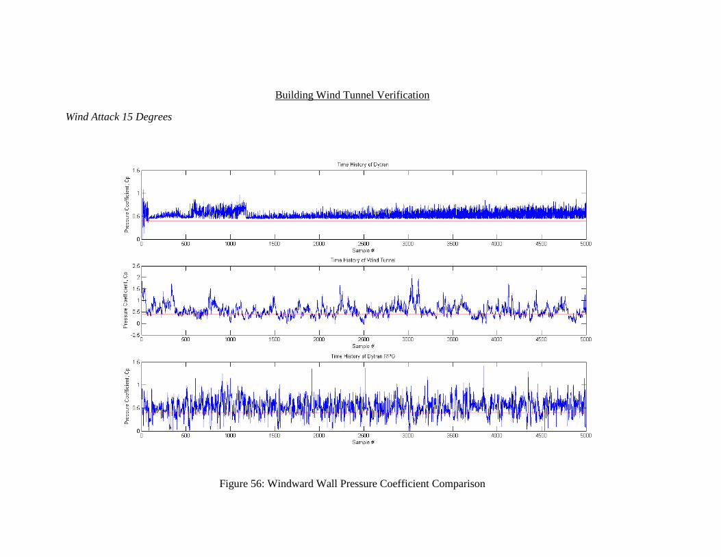
Building Wind Tunnel Verification
Wind Attack 15 Degrees
Figure 56: Windward Wall Pressure Coefficient Comparison

122
Figure 57: Windward Wall PSD Comparison

123
Figure 58: Windward Wall Autocorrelation Coefficient Comparison
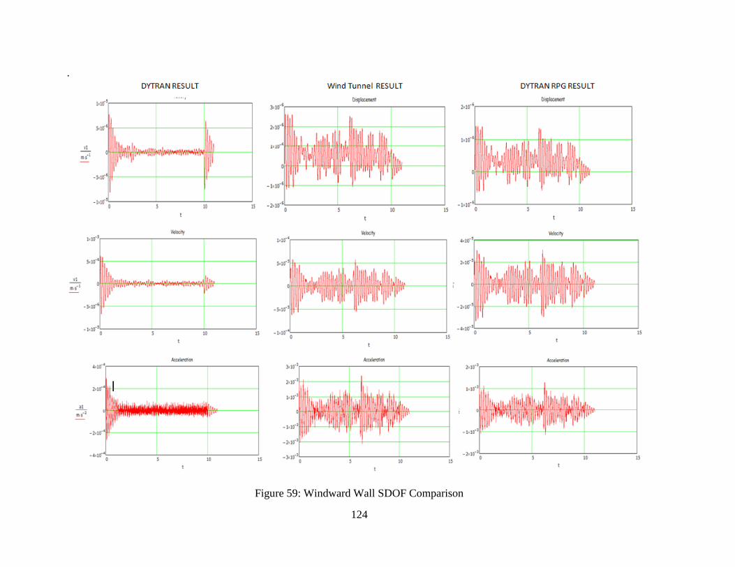
124
.
Figure 59: Windward Wall SDOF Comparison
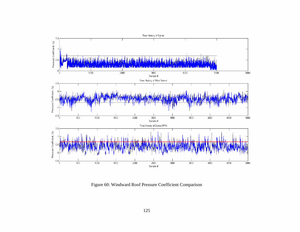
125
Figure 60: Windward Roof Pressure Coefficient Comparison
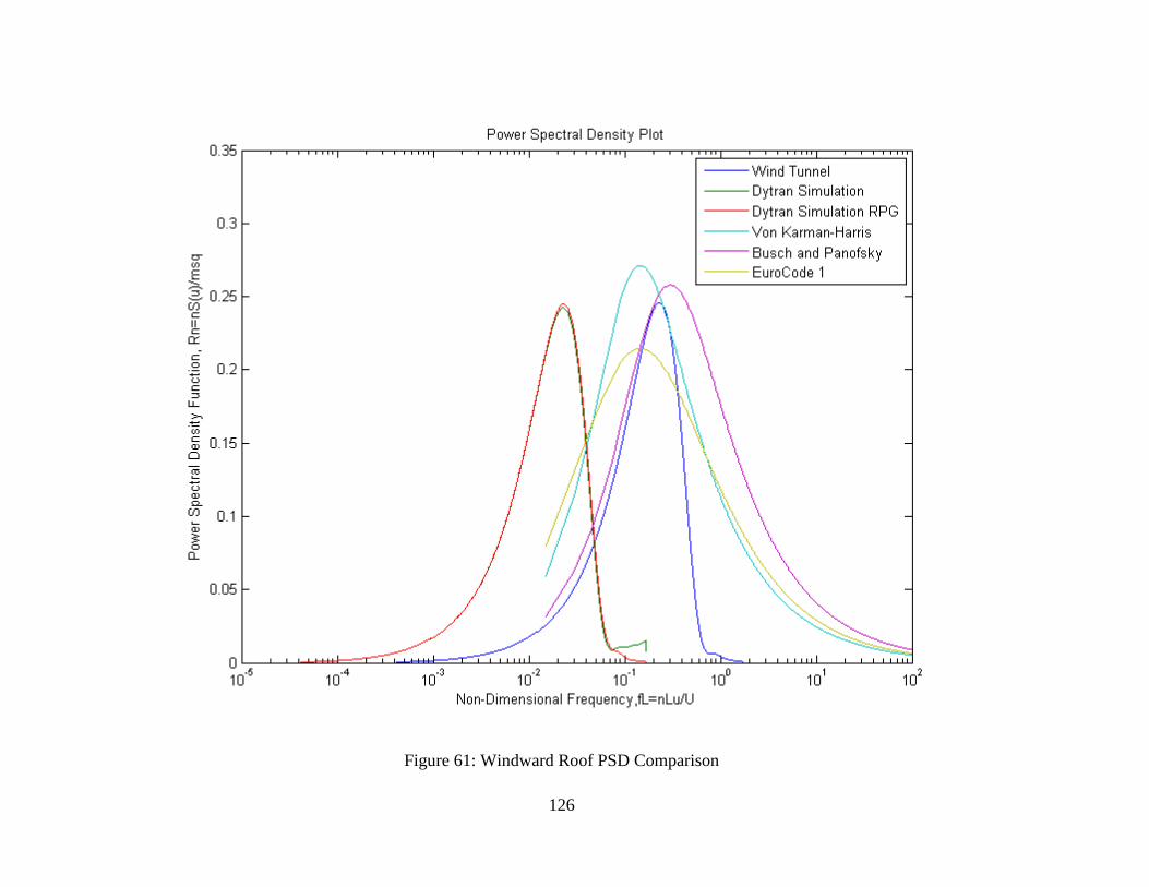
126
Figure 61: Windward Roof PSD Comparison
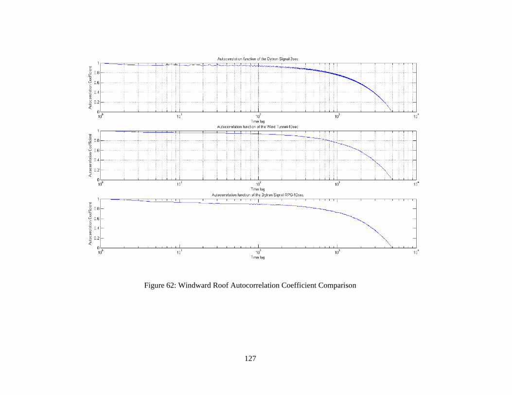
127
Figure 62: Windward Roof Autocorrelation Coefficient Comparison
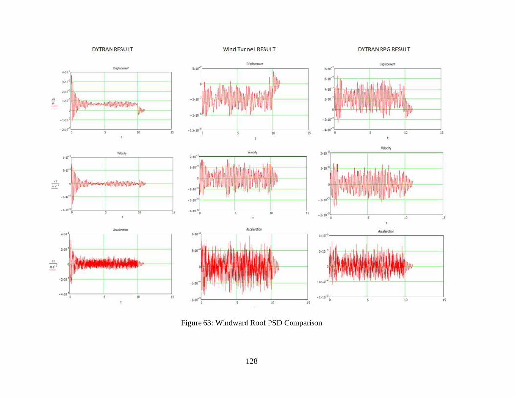
128
Figure 63: Windward Roof PSD Comparison

129
Figure 64: Roof Peak Pressure Coefficient Comparison

130
Figure 65: Roof Peak PSD Comparison

131

132
Figure 66: Roof Peak Autocorrelation Coefficient Comparison
Figure 67: Peak SDOF Comparison

133
Figure 68: Leeward Roof Pressure Coefficient Comparison

134
Figure 69: Leeward Roof PSD Comparison

135
Figure 70: Leeward Roof Autocorrelation Comparison

136
Figure 71: Leeward Roof SDOF Comparison

137
Figure 72: Leeward Wall Pressure Coefficient Comparison

138
Figure 73: Leeward Wall PSD Comparison

139
Figure 74: Leeward Wall Autocorrelation Comparison
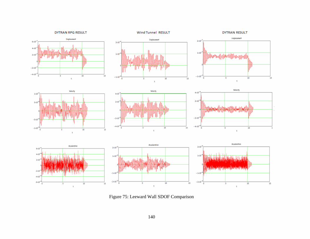
140
Figure 75: Leeward Wall SDOF Comparison

141
Wind Attack 45 Degrees
Figure 76: Windward Wall Pressure Coefficient Comparison

142
Figure 77: Windward Wall PSD Comparison

143
Figure 78: Windward Wall Autocorrelation Comparison

144
Figure 79: Windward Roof Pressure Coefficient Comparison

145
Figure 80: Windward Roof PSD Comparison
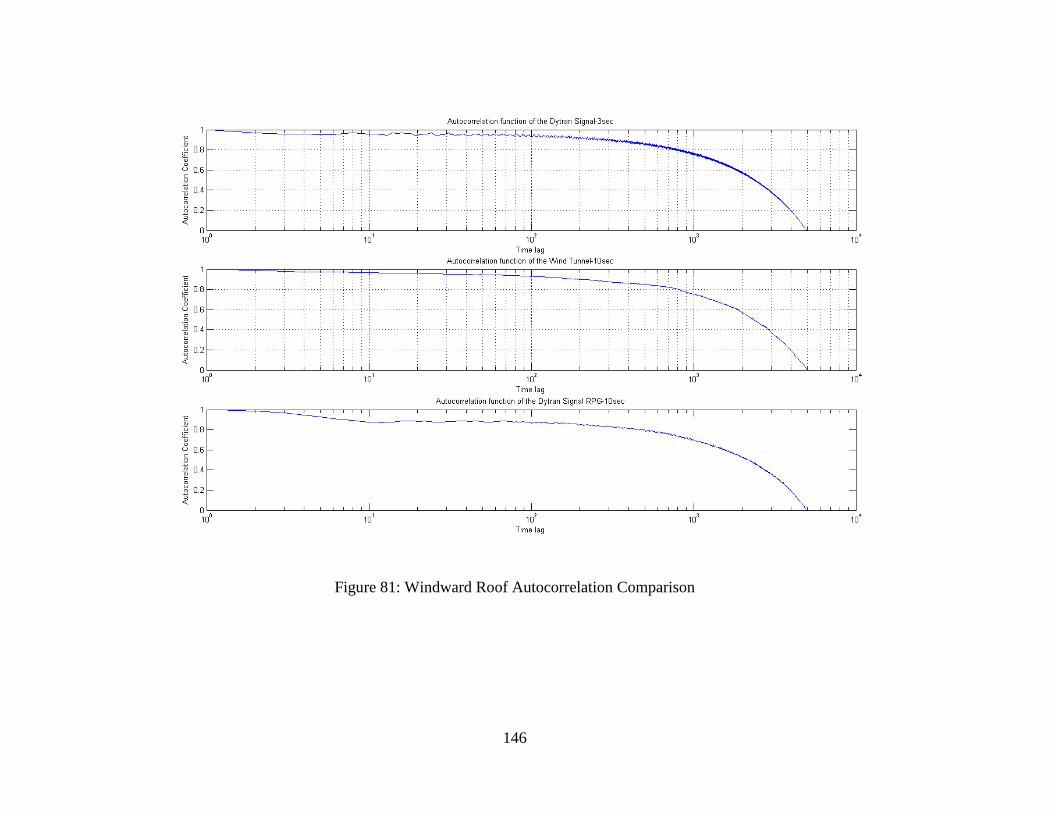
146
Figure 81: Windward Roof Autocorrelation Comparison
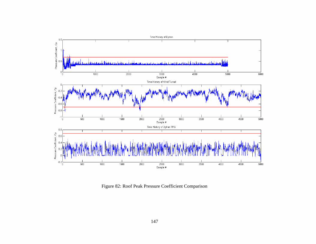
147
Figure 82: Roof Peak Pressure Coefficient Comparison

148
Figure 83: Roof Peak PSD Comparison

149
Figure 84: Roof Peak Autocorrelation Comparison

150
Figure 85: Leeward Wall Pressure Coefficient Comparison
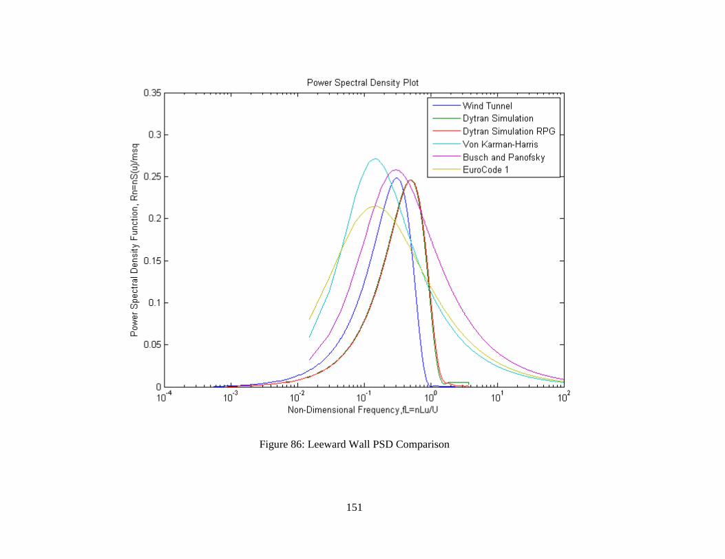
151
Figure 86: Leeward Wall PSD Comparison

152
Figure 87: Leeward Wall Autocorrelation Comparison
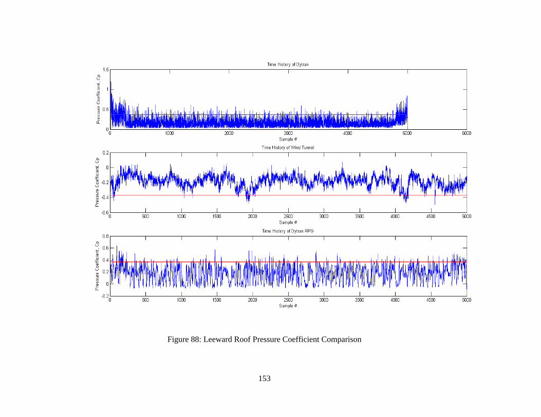
153
Figure 88: Leeward Roof Pressure Coefficient Comparison

154
Figure 89: Leeward Roof PSD Comparison
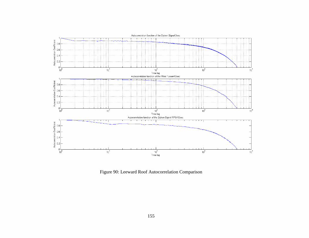
155
Figure 90: Leeward Roof Autocorrelation Comparison

156
Bridge Wave Tank Basin Verification
Figure 91: Test Number 47 Vertical Time History Unfiltered
0 0.5 1 1.5 2 2.5 3 3.5 4-200
0
200
400
600
800
1000
1200
1400
1600Vertical Force Time History Simulation
Time, sec
Forc
e,
N

157
Figure 92: Test Number 47 Filtered
0 100 200 300 400 500 600 700 800-150
-100
-50
0
50
100
150
200
250
300
350Time History of Wave Vertical Force
Sample #, Fs=200Hz
Forc
e,
N

158
Figure 93: Vertical Time History From Test Number 47 Normalized
0 0.5 1 1.5 2 2.5 3 3.5 4-0.5
0
0.5
1
1.5
2Vertical Force Time History Simulation Test 50
Time, sec
Norm
aliz
ed V
ert
ical F
orc
e,
F/p
gH
sA

159
Figure 94: Test Number 47 Horizontal Time History Unfiltered
0 0.5 1 1.5 2 2.5 3 3.5 4-100
-80
-60
-40
-20
0
20
40
60
80Horizontal Force Time History Simulation 1
Time, sec
Forc
e,
N

160
Figure 95: Test Number 47 Filtered
0 0.5 1 1.5 2 2.5 3 3.5 4-20
-15
-10
-5
0
5
10
15
20Horizontal Force Time History Simulation 1
Time, sec
For
ce,
N

161
Figure 96: Horizontal Time History From Test Number 47 Normalized
0 0.5 1 1.5 2 2.5 3 3.5 4-0.8
-0.6
-0.4
-0.2
0
0.2
0.4
0.6Horizontal Force Time History Simulation Test 50
Time, sec
Nor
mal
ized
Hor
izon
tal F
orce
, F
/pgH
sA

162
Figure 97: Vertical Force Time History Test Number 50 Filtered
0 0.5 1 1.5 2 2.5 3 3.5 4-200
-100
0
100
200
300
400Vertical Force Time History Simulation Test 50
Time, sec
Forc
e,
N

163
Figure 98: Normalized Vertical Force Time History
0 0.5 1 1.5 2 2.5 3 3.5 4-1
-0.5
0
0.5
1
1.5
2Vertical Pressure Time History Simulation Test 50
Time, sec
Norm
aliz
ed V
ert
ical P
ressure
, P
/pgH
s

164
Figure 99: Horizontal Force Time History Test Number 50 Filtered
0 0.5 1 1.5 2 2.5 3 3.5 4-20
-15
-10
-5
0
5
10Horizontal Force Time History Simulation Test 50
Time, sec
Forc
e,
N

165
Figure 100: Normalized Horizontal Force Time History
0 0.5 1 1.5 2 2.5 3 3.5 4-0.6
-0.5
-0.4
-0.3
-0.2
-0.1
0
0.1
0.2
0.3Horizontal Force Time History Simulation Test 50
Time, sec
Norm
alized H
orizonta
l F
orc
e,
F/p
gH
sA
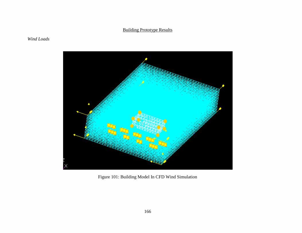
166
Building Prototype Results
Wind Loads
Figure 101: Building Model In CFD Wind Simulation

167
Figure 102: Third Floor Leeward Wall Nodal Time History
0 500 1000 1500 2000 2500 3000 3500 4000 4500 5000-0.4
-0.2
0
0.2
0.4
0.6
0.8
1
1.2
1.4Time History of Dytran RPG Node 210
Sample #, Fs=500Hz
Pre
ssure
Coeff
icie
nt,
Cp

168
Figure 103: Third Floor Leeward Wall PSD
10-4
10-3
10-2
10-1
100
101
102
0
0.05
0.1
0.15
0.2
0.25
0.3
0.35Power Spectral Density Plot
Non-Dimensional Frequency,fL=nLu/U
Pow
er
Spectr
al D
ensity F
unction,
Rn=
nS
(u)/
msq
Dytran Simulation
Von Karman-Harris
Busch and Panofsky
EuroCode 1

169
Figure 104: First Floor Windward Wall Nodal Time History
0 500 1000 1500 2000 2500 3000 3500 4000 4500 5000-0.5
0
0.5
1
1.5
2Time History of Dytran RPG Node 119
Sample #, Fs=500Hz
Pre
ssur
e C
oeff
icie
nt,
Cp

170
Figure 105: First Floor Windward Wall PSD
10-3
10-2
10-1
100
101
102
0
0.05
0.1
0.15
0.2
0.25
0.3
0.35Power Spectral Density Plot
Non-Dimensional Frequency,fL=nLu/U
Pow
er
Spectr
al D
ensity F
unction,
Rn=
nS
(u)/
msq
Dytran Simulation
Von Karman-Harris
Busch and Panofsky
EuroCode 1

171
Wave Loads .
Figure 106: Column Model In CFD Wave Simulation
Figure 107: Input shape of Setup Wave for Column Wave Simulations.
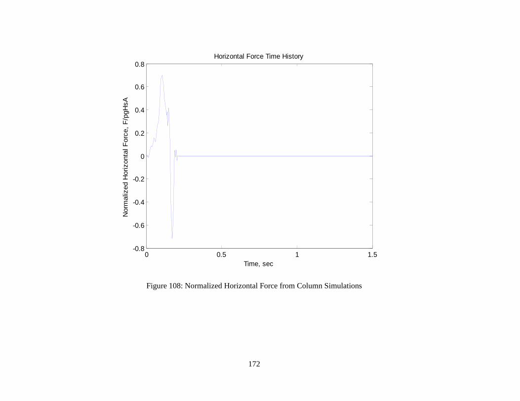
172
Figure 108: Normalized Horizontal Force from Column Simulations
0 0.5 1 1.5-0.8
-0.6
-0.4
-0.2
0
0.2
0.4
0.6
0.8Horizontal Force Time History
Time, sec
Norm
alized H
orizonta
l F
orc
e,
F/p
gH
sA

173
Figure 109: Normalized Vertical Force from Column Simulations
0 0.5 1 1.5-0.02
0
0.02
0.04
0.06
0.08
0.1
0.12Vertical Force Time History
Time, sec
Norm
aliz
ed V
ert
ical F
orc
e,
F/p
gH
sA
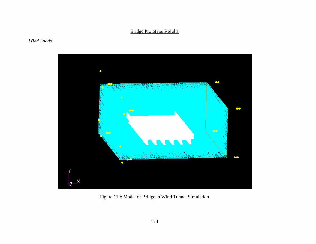
174
Bridge Prototype Results
Wind Loads
Figure 110: Model of Bridge in Wind Tunnel Simulation

175
Figure 111: Windward Barrier Force/Pressure Records

176
Figure 112: Windward Barrier Force/Pressure RPG Record
0 5 10 15 20 25-0.2
0
0.2
0.4
0.6
0.8
1
1.2Force Time History Simulation RPG
Time, sec
Forc
e,
N

177
Figure 113: Windward Barrier Force/Pressure RPG Record PSD Comparison

178
Figure 114: Windward Barrier Force/Pressure RPG Record Autocorrelation Coefficient
100
101
102
103
0
0.1
0.2
0.3
0.4
0.5
0.6
0.7
0.8
0.9
1Autocorrelation function of the Dytran Signal-1.5sec
Time lag
Aut
ocor
rela
tion
Coe
ffic
ient

179
Figure 115: Top Deck Force/Pressure Records
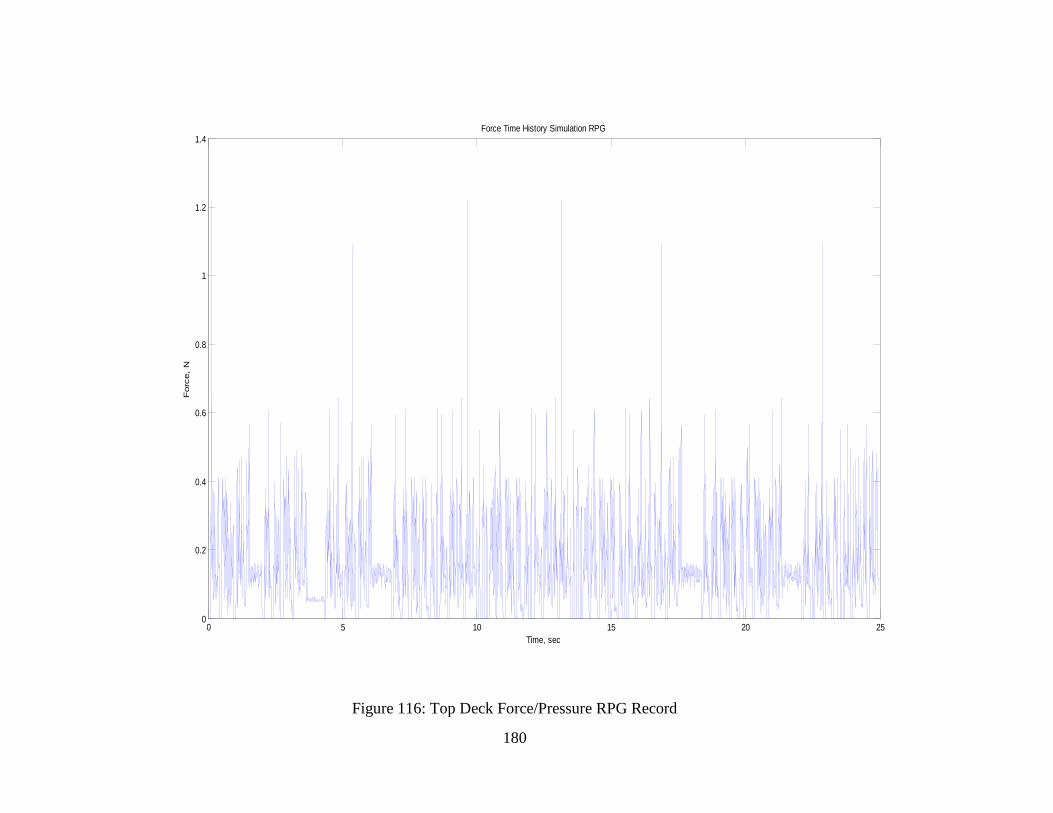
180
Figure 116: Top Deck Force/Pressure RPG Record
0 5 10 15 20 250
0.2
0.4
0.6
0.8
1
1.2
1.4Force Time History Simulation RPG
Time, sec
Forc
e,
N
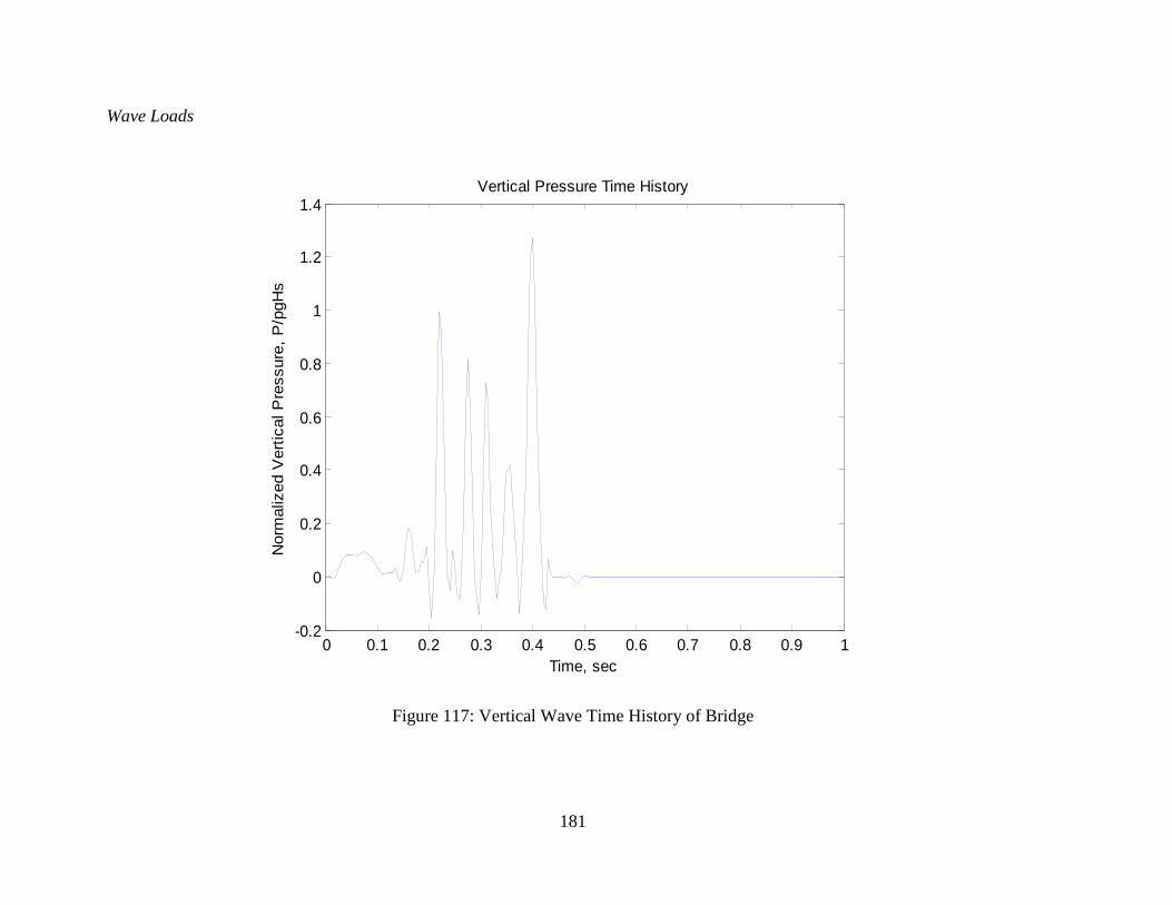
181
Wave Loads
Figure 117: Vertical Wave Time History of Bridge
0 0.1 0.2 0.3 0.4 0.5 0.6 0.7 0.8 0.9 1-0.2
0
0.2
0.4
0.6
0.8
1
1.2
1.4Vertical Pressure Time History
Time, sec
Norm
alized V
ert
ical P
ressure
, P
/pgH
s

182
Figure 118: Horizontal Wave Time History of Bridge
0 50 100 150 200 250-5
-4
-3
-2
-1
0
1
2Horizontal Force Time History
Time, sec
Norm
aliz
ed H
orizonta
l F
orc
e,
F/p
gH
sA

REFERENCES
Batts, M.E., Cordes, M.R., Russell, L.R., Shaver, J.R., Simiu, E. (1980). Hurricane wind speeds
in the United States. National Bureau of Standards, Report Number BSS-124, US
Department of Commerce, 50pp.
Cuomo, G,, Allsop, W. and Takahashi, S. (2010), Scaling Wave Impact Pressures on vertical
walls, Coastal Engineering, Volume (57), 604-609
Cuomo, G,, Allsop, W. and Trindelli, M. (2007), Wave-in-Deck Loads on Exposed Jetties,
Coastal Engineering, Volume (54), Issue 9, 657-679
Chopra, Anil (1995), Dynamics of Structures Theory and Applications to Earthquake
Engineering, Prentice Hall, ISBN 0-13-855214-2, 729 pages
Daniels, Richard (1974), Approximation Methods for Electronic Filter Design, New York:
McGraw—Hill. ISBN 0-07-015308-6, p. 896
David W. Wang,* Douglas A. Mitchell, William J. Teague, Ewa Jarosz, Mark S. Hulbert (2005),
Extreme Waves Under Hurricane Ivan, Science 5 August 2005: Vol. 309. no. 5736, p.
896
Dagnew, Agerneh, Bitsuamalk, Girma and Merricak, Ryan, (2009), Computational Evaluation of
wind pressures on tall buildings, 11th Americas Conference on Wind Engineering-San
Juan Puerto Rico, June 22-26, 2009
Donea, J. and Huerta, A. (2003), Finite Element Methods for Flow Problems, John Wiley and
Sons, ISBN 3-2103-01184-3020 , 350 pages
Dyrbye, Claȅs and Hansen, Svend (1997), Wind Loads on Structures, John Wiley and Sons,
ISBN 0-471-95651, 229 pages
Dytran Theory Manual r1 (2008), MSC Software Corporation, www.mscsoftware.com

184
Franke, J., Hirsch, C., Jensen, A.G., Krüs, H.W., Schatzmann, M., Westbury, P.S., Miles, S.D.,
Wisse, J.A., Wright, N.G., (2004). Recommendations on the use of CFD in wind
engineering. Proceedings of the International Conference on Urban Wind Engineering
and Building Aerodynamics, in: van Beeck JPAJ (Ed.), COST Action C14, Impact of
Wind and Storm on City Life Built Environment, von Karman Institute, Sint-Genesius-
Rode, Belgium, 5 - 7 May 2004.
Holmes, John D. (2001), Wind Loading of Structures, Spoon Press, ISBN 0-419-24610 , 356
pages
Kinsman, Blair (1984), Wind waves: their generation and propagation on the ocean surface,
Dover Publications, ISBN 0-486-49511-6 , 704 pages
Kiureghian, D. and Ditlevesen, O. (2009), ―Aleatory or epistemic? Does it matter?‖, Structural
Safety, 31, 105-112
Kiureghan, Armen and Liu, Pei-Ling (1986), Multivariate distribution models with prescribed
marginals and covariances, Probability Engineering Mechanics, Vol. 1 (2), 105-112
Jelesnianski, C. P., J. Chen, and W. A. Shaffer, (1992): SLOSH: Sea, lake, and overland surges
from hurricanes. NOAA Technical Report NWS 48, National Oceanic and Atmospheric
Administration, U. S. Department of Commerce, 71 pp. (Scanning courtesy of NOAA's
NOS's Coastal Service's Center
Lin, Y.K. and Cai G.Q. (1995), Probabilistic Structural Dynamics, McGraw-Hill, ISBN 0-07-
038038-4, 476 pages
Main J. A. and Fritz W. A. (2006). "Database-Assisted Design for Wind: Concepts, Software, and
Examples for Rigid and Flexible Buildings," NIST Building Science Series 180.
Mara, T.G. and King, J.P.C. (2008). "A Study of Wind Effects for Anna Marie Bridge Design
Alternatives Anna Marie Island, Florida". BLWT-SS74-2008. December 2008.
Masters, F.J., Gurler, K.R., Biggerstaff, M., Knupp, K. and Coulbourne, W.L. (2010). "The
Digital Hurricane Consortium: An Adaptive Mesonet to Monitor Wind, Surge, Wave and

185
Rainfall Intensities and Damage at Landfall". 2010 Structures Congress. Orlando, Fl
2010.
Masters, F.J., Gurler, K.R. and Prevatt, D.O. (2010). "Advancing Performance Based Design
through Full-Scale Simulation of Wind Water and Structural Interaction". 2010
Structures Congress. Orlando, Fl 2010.
Petrini, F, Ciampoli, M and Augusti, G. (2009), A probabilistic framework for Performance
Based Wind Engineering: EACWE 5 Florence, Italy, July 19-23 2009
Phan, Long and Simiu, Emil (2007), Methodology for Development of Design Criteria for Joint
Hurricane Wind Speed and Storm Surge Events: NIST Technical Note 1482, April 2007
Prevatt, David, Datin, Peter (2009), Performance Based Wind Engineering: Interaction of
Hurricanes with Residential Structures, Proceedings of 2009 NSF Engineering Research
and Innovation Conference, Honolulu, Hawaii
Robertson, A. P., & Glass, A. G., (1988). The Silsoe structures building - its design,
instrumentation and research facilities. AFRC Inst. Engng. Res., Silsoe, Div. Note DN
1482.
Robertson, Ian, Riggs, H., Yim, Solomon and Young, Yin. (2007) Lessons from Hurricane
Katrina Storm Surge on Bridges and Buildings. Journal of Waterway, Port, Coastal and
Ocean Engineering, ASCE, Vol. (133), No. 6, 463-479.
Sheppard, Max and Marin, Justin (2009) Wave Loading On Bridge Decks: Final report. FDOT
Report BD 545-58. UF Number 00056675. 177 pages.
Simiu, Emil and Scanlan, Robert (1986), Wind Effects on Structures 2nd
Edition, John Wiley and
Sons, ISBN 0-471-86613 , 589 pages
Simiu E, Sadek F, Whalen TM, Jang S, Lu L-W, Diniz SMC, Grazini A, Riley MA., (2008)
Achieving safer and more economical buildings through database-assisted, reliability-
based design for wind., Journal of Wind Engineering and Industrial Aerodynamics.
2003;91(12-15):1587-1611.

186
Tschanz, T. and Davenport, A.G. (1983) The base balance technique for the determination of
dynamic wind loads, Journal of Wind Engineering and Industrial Aerodynamics. 1983;
volume 10 (1-3):429-439.
Vickery, P. J., Skerlj, P. F., Steckley, A. C., and Twisdale, L. A. (2000). ‗‗Simulation of
Hurricane Risk Using Empirical track model.‘‘, Journal of Structural Engineering, ASCE,
126(10), 1203–1222.
Whittaker, Andrew (2005), Performance-Based Engineering of Buildings and Infrastructure for
Extreme Loadings, Dover Publications, ISBN 0-486-49511-6 , 8 pages
Wu C. S., Taylor A.T., Chen J,, Shaffer W., (2003), ―Tropical Cyclone Forcing of Ocean Waves‖,
Conference on Coastal Atmospheric and Oceanic Predication and Processes, Seattle,
Washington, 62-64
Yim, S.C., Cox, D.T. and Park M.M. (2009), Experimental and Computational Activities at the
Oregon State University NEES Tsunami Research Facility, Science of Tsunami Hazards,
Vol 28, No. 1, 14 pages
Yu, Bo, Chowdhurry, Arindam and Masters, Forrest (2008), Hurricane Wind Power Spectra,
Cospectra, and Integral Length Scales, Boundary Layer Meteorology, Vol 129, pg 411-
430