Embed Size (px)
Citation preview

COMPUTATIONAL FLUID DYNAMIC ANALYSIS OF
THE PURIFICATION PROCESS OF THE
NEUTRINO DETECTOR KAMLAND
by
AARON MITCHELL COSSEY
A THESIS
Submitted in partial fulfillment of the requirements
for the degree of Master of Sciences in the
Department of Mechanical Engineering
in the Graduate School of
The University of Alabama
TUSCALOOSA, ALABAMA
2009

Copyright Aaron Mitchell Cossey 2009
ALL RIGHTS RESERVED

ii
ABSTRACT
A simplified two-dimensional finite volume axisymmetric mesh was constructed that
represented the geometry of the Kamioka Liquid scintillator Anti-Neutrino Detector
(KamLAND) experiment in order to perform a computational fluid dynamics (CFD) analysis of
the purification process of the liquid scintillator (LS). 1,000 tons of the LS, contained within a
13 meter-diameter spherical balloon in the center of the detector, is purified in a continuous
process where the LS is simultaneously withdrawn from the bottom and replaced at the top of the
detector. During this purification process, the interface between the newly purified and
unpurified LS is not stratified horizontally as expected, but instead mixing is observed, reducing
the efficiency of the process and preventing the desired level of purification throughout the LS.
Using the commercial CFD software FLUENT, the purification process of the experiment
was simulated based on the conditions and data previously recorded during the purification
phase. The CFD analysis of the experiment was modeled as a transient problem, with flow and
heat transfer solved. The phenomenon of natural convection was modeled using the Boussinesq
approximation. The volume of fraction (VOF) method was used to track the interaction between
the purified and unpurified liquids in the simulation.
The CFD simulation will be used to test proposed improvements to the purification
process for future purification programs of KamLAND. The CFD simulation will serve as a
guide to test these improvements and improve the efficiency of the process.

iii
DEDICATION
I would like to dedicate this thesis to all of my friends and family who provided me with
their support to the very end. Without their support, I do not know if I would have ever been
able to finish this thesis.

iv
ACKNOWLEDGMENTS
I would like to thank all of my colleagues, friends, and faculty members who have helped
me with this project. In particular, I would like to thank my supervisor Dr. Keith Woodbury for
his support and patience, even when I did not think that I would ever finish. His knowledge and
suggestions for my CFD simulation were of great benefit to me. I would like to thank the
Physics Department of the University of Alabama’s members of the KamLAND Collaboration,
Dr. Andreas Piepke and Greg Keefer, for the opportunity to work on this project.
I would also like to thank Dr. Michael Freeman and Dr. Will Schreiber for serving on my
thesis committee and providing their recommendations.

v
LIST OF ABBREVIATIONS AND SYMBOLS
BO buffer oil of detector
mBq milli-Bequerel, decay / 1,000 second
CAD Computer Aided Drawing
CFD Computational Fluid Dynamics
ρ density, kg / m3
ev electron anti-neutrino
g gravitational constant, 9.81 m/s2
ID inner detector
KamLAND Kamioka Liquid scintillator Anti-Neutrino Detector
K Kelvin degree
k thermal conductivity
LS liquid scintillator of detector
mass transfer rate
m meter
µm micrometer or 10-6
meter
mm millimeter or 10-3
meter
OD outer detector
PMTs photomultiplier tubes
r dimensional radial coordinate
Sh volumetric heat rate, W / m3

vi
UDF user defined function
vx dimensional axial velocity
vr dimensional radial velocity
vz swirl velocity
ν kinematic viscosity
VOF volume of fluid
x dimensional axial coordinate

vii
CONTENTS
ABSTRACT .................................................................................................................................... ii
DEDICATION ............................................................................................................................... iii
ACKNOWLEDGMENTS ............................................................................................................. iv
LIST OF ABBREVIATIONS AND SYMBOLS ........................................................................... v
LIST OF TABLES .......................................................................................................................... x
LIST OF FIGURES ....................................................................................................................... xi
CHAPTER 1 INTRODUCTION ................................................................................................. 1
1.1 A Brief Description of KamLAND ....................................................................................... 1
1.2 The Detector of KamLAND ................................................................................................. 2
1.3 Purification System of the Detector ...................................................................................... 4
1.4 Objective of Project .............................................................................................................. 8
1.5 Scope of Project .................................................................................................................... 8
CHAPTER 2 CFD PHYSICAL MODELS ............................................................................... 10
2.1 CFD Introduction ................................................................................................................ 10
2.2 Governing Equations .......................................................................................................... 11
2.2.1 Assumptions to Simply the CFD Simulation ............................................................... 12
2.2.2 The Mass Conservation and Momentum Equations .................................................... 12

viii
2.2.3 The Energy Equation and Heat Transfer Theory ......................................................... 14
2.2.4 Natural Convection and the Boussinesq Model ........................................................... 15
2.2.5 Volume of Fluid (VOF) Theory ................................................................................... 17
CHAPTER 3 CFD KAMLAND MODEL ................................................................................ 19
3.1 Steps in Solving CFD Problem ........................................................................................... 19
3.2 The Modeling Goals ........................................................................................................... 19
3.3 Creating the Model Geometry ............................................................................................ 20
3.3.1 Simplyfying the KamLAND Geometry ....................................................................... 22
3.3.2 Meshing the KamLAND Geometry ............................................................................. 23
3.3.3 Description of the Grid ................................................................................................ 28
3.4 Pre-Processing of FLUENT ................................................................................................ 29
3.4.1 Reading in the Grid ...................................................................................................... 29
3.4.2 Defining the Material Properties and Boundary Conditions ........................................ 29
3.4.3 Enabling the Desired Physical Models ........................................................................ 33
3.4.5 Initializing the Solution................................................................................................ 34
3.4.6 Selecting the Solution Controls ................................................................................... 36
3.5 Computing the Solution of FLUENT ................................................................................. 40
3.6 Post-Processing the Results of FLUENT ............................................................................ 42

ix
CHAPTER 4 RESULTS AND DISCUSSION ......................................................................... 43
CHAPTER 5 CONCLUSIONS ................................................................................................. 52
REFERENCES ............................................................................................................................. 55
APPENDIX A KAMLAND COLLABORATION ................................................................ A-1
APPENDIX B METHOD OF TRACKING 222
RN DAUGHTERS....................................... B-1
APPENDIX C MATERIALS PARAMETERS ..................................................................... C-1
APPENDIX D BOUNDARY CONDITIONS ....................................................................... D-1
APPENDIX E USER DEFINED FUNCTION TEMPERATURE PROFILE ....................... E-1
APPENDIX F KAMLAND CFD WORK SHEET ................................................................ F-1

x
LIST OF TABLES
Table 1-1. Background activities in KamLAND before and after purification. ............................. 6
Table 3-1. Details of the CFD mesh created in GAMBIT. ........................................................... 28
Table F-1. KamLAND_2Dv10 Work Sheet. ............................................................................... F-1

xi
LIST OF FIGURES
Figure 1-1. An illustration of the KamLAND hall and access tunnels. ......................................... 3
Figure 1-2. Conceptual drawing of KamLAND. ............................................................................ 4
Figure 1-3. Purified LS volume and flow rate over 1st purification campaign. ............................. 5
Figure 1-4. Distinct separation of old and new LS during first purification phase. ....................... 7
Figure 3-1. KamLAND detailed schematic. ................................................................................. 20
Figure 3-2. KamLAND geometry created using Pro/E. ............................................................... 21
Figure 3-3. GAMBIT geometry created from IGES file. ............................................................. 22
Figure 3-4. GAMBIT simplified geometry. ................................................................................. 23
Figure 3-5. Simple geometry of model used to test the grid resolution required. ........................ 25
Figure 3-6. Mesh used in KamLAND CFD simulation. .............................................................. 25
Figure 3-7. Enlarged view of the boundary layer used on the walls of the LS domain. .............. 26
Figure 3-8. Enlarged view of skewed cells in outlet pipe. ........................................................... 27
Figure 3-9. Density and mass flow rate of LS over the course of the first purification process. . 30
Figure 3-10. Plots of temperature versus time of four elevation levels within the OD. ............... 31
Figure 3-11. Polynomial trendline of OD temperature versus distance along z-axis. .................. 32
Figure 3-12. Measured temperature (°C) distribution in KamLAND. ......................................... 35
Figure 3-13. Initial temperature distribution calculated by FLUENT. ......................................... 35
Figure 3-14. Temperature distribution of solution with only the energy equation solved. .......... 37
Figure 3-15. Temperature distribution with energy and flow equations coupled. ....................... 37
Figure 3-16. Temperature distribution in simple CFD model with only energy solved. ............. 38
xii
Figure 3-17. Temperature distribution in simple CFD model with energy and flow solved. ...... 39
Figure 3-18. KamLAND geometry partitioned for parallel computing. ...................................... 40
Figure 3-19. Scaled residuals plot of the KamLAND CFD simulation. ...................................... 41
Figure 4-1. Montage of KamLAND after one day of purification. .............................................. 44
Figure 4-2. Montage of KamLAND after one week of purification. ........................................... 44
Figure 4-3. Montage of KamLAND after two weeks of purification. .......................................... 45
Figure 4-4. Montage of KamLAND after three weeks of purification. ........................................ 45
Figure 4-5. Montage of KamLAND after four weeks of purification. ......................................... 46
Figure 4-6. Montage of KamLAND after five weeks of purification. ......................................... 46
Figure 4-7. Montage of KamLAND after six weeks of purification. ........................................... 47
Figure 4-8. Montage of KamLAND after seven weeks of purification. ...................................... 47
Figure 4-9. Montage of KamLAND after eight weeks of purification......................................... 48
Figure 4-10. Montage of KamLAND after nine weeks of purification. ....................................... 48
Figure 4-11. Montage of KamLAND CFD simulation temperature profile. ............................... 49
Figure 4-12. Spacial distribution of BiPo events with the fiducial volume cut removed. ........... 51
Figure B-1. Decay scheme for 222
Rn. ......................................................................................... B-2
Figure B-2. Pairs of events that satisfy energy selection cut for 214
Bi-214
Po events. .................. B-3
Figure B-3. Dots representing 214
Bi-214
Po event pair from the decay of 222
Rn in the detector. . B-4

1
CHAPTER 1 INTRODUCTION
1.1 A Brief Description of KamLAND
The Kamioka Liquid scintillator Anti-Neutrino Detector (KamLAND) is an experiment at
the Kamioka Observatory, an underground neutrino observatory near Toyama, Japan, that was
built to detect electron anti-neutrinos ( ev ) (KamLAND Wiki). The group of international
scientists, professors, and students from the United States (including the Physics Department of
the University of Alabama), Japan, and Europe working on the experiment is known as the
KamLAND Collaboration and is listed in Appendix A. The KamLAND Collaboration has
reported that the experiment has determined the associated oscillation parameter Δ m2
21 to
unprecedented precision, has helped constrain the neutrino mixing angle θ 12, and has explored
the potential application of neutrinos as a geophysical probe. The detector is currently
undergoing an upgrade to the purification process which will enable KamLAND to execute a low
energy solar neutrino program to detect 7Be solar neutrinos in parallel with this already highly
fruitful anti-neutrino program (KamLAND Collaboration).
The KamLAND project was proposed in 1994. In 1997, the full budget was funded by
the Japanese Ministry of Education. In 1999 the United States Department of Energy approved
the US-KamLAND proposal. Following a five year period for construction of the detector and
the underground facility, KamLAND was launched into data-taking on January 22, 2002. The
main objectives of KamLAND are to aim at studying reactor electron anti-neutrino oscillations
with more than 100 kilometer baseline, simultaneously searching for neutrinos from both

2
terrestrial and solar sources. Data taking has been consistently gathered since March 2002
(Suzuki et al., 2005).
During the summer of 2007, the first upgraded purification process of the liquid
scintillator (LS) used in the detection of the solar neutrinos encountered difficulties in attaining
the desired reduction of the levels of the radioactive impurities that interferes with low level
energy detection. During the purification process, the liquid scintillator is purified in a
continuous process where LS is simultaneously withdrawn from the bottom and replaced at the
top of the detector. The interface between the newly purified and unpurified LS was not
stratified horizontally as expected due to unaccounted for mixing inside of the detector. This
mixing reduced the efficiency of the process and prevented the desired level of purification
throughout the LS. There is no understanding of how the flow field present during the
purification process affects this mixing.
1.2 The Detector of KamLAND
The detector was built in the Kamioka mine, 1,000 meters under the top of Mt.
Ikenoyama, which was the site of the old Kamiokande: the 3000 cubic meter water Cerenkov
detector which played a leading role in the study of neutrinos produced via cosmic rays and also
helped to pioneer the subject of neutrino astronomy. After dismantling the Kamiokande
detector, the rock cavity was enlarged to be 20 meters in diameter and 20 meters in height. An
illustration of the detector within the mine is displayed in Figure 1-1. Background events for the
neutrino detection are caused by undesired radioactive particles which come into the scintillator
from the outside or inside of the detector. To guard against external radiation, the detector
consists of a cylinder containing a series of concentric spherical shells. KamLAND consists of
three distinct regions: the inner detector, the buffer region, and the outer detector. The inner

3
neutrino detector is 1000 tons of ultra pure liquid scintillator (LS) located at the center of the
detector. The KamLAND LS is a chemical cocktail of 80% dodecane, 20% 1,2,4-
trimethylbenzene, and 1.52 g/liter 2,5-diphenyloxazole as a fluor.
Figure 1-1. An illustration of the KamLAND hall and access tunnels.
The scintillator is housed in a 13 meter-diameter spherical balloon made of 2 layers of nylon
with a total thickness of 135 µm, and supported by a cargo net structure at the top of a stainless
steel vessel. This balloon system hangs in an 18 meter-diameter stainless steel spherical vessel.
A buffer oil (BO) mixture of dodecane and isoparaffin fills the volume between the stainless
steel vessel and the balloon in the buffer region. The density of the BO is kept at 0.04% lower
than that of the LS, increasing its buoyancy, to reduce the weight-load on the balloon. The entire
inner surface of the vessel, the inner detector (ID), is covered by an array of a total of 1879
photomultiplier tubes (PMTs). The fluor in the scintillator is excited by the energy loss of the

4
radiation generated from particle interactions, and emits light which is detected by the PMTs. A
3 millimeter thick acrylic barrier at 16.6 meter-diameter prevents radon emanating from PMT
glasses from invading into the LS. This central detector stands in a cylindrical rock cavity. The
volume between the sphere vessel and the cavity is filled with roughly 3200 cubic meters of pure
water where 225 PMTs are placed to detect cosmic-ray muons by their Cerenkov light. This
outer detector (OD) absorbs γ-rays and neutrons from surrounding rock (Suzuki et al. 2005).
Figure 1-2 shows a conceptual drawing of the detector and labels the major components.
Figure 1-2. Conceptual drawing of KamLAND.
1.3 Purification System of the Detector
One kiloton of liquid scintillator is necessary in KamLAND because high statistics is
essential to the observation of neutrinos. In addition, the sensitivity for the difference in the
squared-mass of the neutrino mass states involved, Δ m2, strongly depends on the observed
neutrinos. Therefore, better energy resolution as well as a low background environment is

5
essential for the experiment and to realize this, very low radioactive impurities for the low
background experiment and high light yield for a good energy resolution (Tajima 2003). Lower
background levels are required to detect solar neutrinos, so a new purification system was
designed and tested.
Two methods were adopted for the new purification system: distillation for metallic or
ionic chemicals, such as 40
K, and purging for gaseous chemicals, such as 85
Kr. The purification
apparatus consisted of two storage tanks, three sets of distillation columns, and purge columns
with an ultra-pure N2 generator. The three sets of distillation columns were for each of the three
chemical components of the LS.
In May of 2007, the first purification campaign was started and ended in the beginning of
August of 2007. The volumetric amount and flow rate of LS is shown in Figure 1-3 over the
course of the purification campaign. LS was simultaneously withdrawn from the bottom plug of
the balloon to be purified and then filled back into KamLAND from the top.
Figure 1-3. Purified LS volume and flow rate over 1st purification campaign.

6
During the purification, reduction factors of the radioactive concentrations were not as large as
expected: one reason attributed was that the original unpurified scintillator and purified
scintillator started mixing together. This was observed by tracing the movement of 222
Rn
daughters through 214
Bi-214
Po coincidence events. This process of tracking is explained in more
detail in Appendix B. Another possibility was that the reduction factor itself in the purification
apparatus appeared less than what was expected from small scale experiments (Kishimoto 2007).
The concentrations of the radioactive impurities before and after the purification campaign are
displayed in Table 1-1 as collected by the KamLAND Collaboration.
Table 1-1. Background activities in KamLAND before and after purification.
Isotope Before [Bq/m3] After (Upper) [Bq/m
3] After (Lower) [Bq/m
3] Required [ ]
210Bi ) × 10
-2 (2 ± 1) × 10
-4 (1.0 ± 0.1) × 10
-2 10
-6
40K (4.4 ± 0.4) × 10
-5 NA (1.3 ± 0.1) × 10
-5 10
-6
85Kr ) × 10
-1 ) × 10
-2 ) × 10
-1 10
-5~-6
222Rn 2.8 × 10
-8 1 × 10
-4 1 × 10
-4 < 10
-3
To try to deal with the issue, the density and the temperature of the last 173 cubic meters of
purified LS was changed: Δρ = -0.03% and ΔT = +1.0K. These changes were made to provide a
more distinct separation between the new and old LS with the density and temperature and
resulted in the two layers: upper layer (z > 4 m) and lower part (z > 2m) (Kishimoto 2007). This
defined interface between the new and old LS can be seen in Figure 1-4, where the scale on the
right has units of mBq/m3. The dark blue area above the 3.5 meter border line has low energy

7
events occurring and indicates the newly purified LS. The desired purification is one where the
interface between the old and new LS remains stratified (horizontal), so that no mixing occurs
and only old LS is withdrawn from the detector.
Figure 1-4. Distinct separation of old and new LS during first purification phase.
The reduction in the level of radioactive impurities during the first purification campaign was not
sufficient to be able to observe the low energy 7Be solar neutrinos.
After the failure of the first purification campaign, steps were taken to upgrade some of
the purification apparatus in preparation for the second purification campaign. It was hoped that
with the upgraded control devices, more stringent temperature control and more careful
adjustment of the liquid scintillator density would keep the new and old liquid scintillator
boundary, minimizing mixing. In addition to the upgrades, purification parameters were

8
searched again to reduce the radioactive chemical much more effectively and use their values for
the next purification campaign. It was also decided that for the second purification that the
filling would occur from the bottom in the hopes of keep the interface stratified between the old
and new LS. The second purification campaign occurred from June of 2008 to December of
2008, and again due to the presence of mixing, the desired reduced concentrations of the
radioactive impurities were not met.
1.4 Objective of Project
It is the aim of this project to develop a computational fluid dynamics (CFD) simulation
of the detector using the commercial CFD software ANSYS®
FLUENT to accurately simulate
the mixing observed during this first purification process. From this CFD simulation, it is hoped
that an efficient purification process can be developed to minimize the amount of mixing
occurring, thus obtaining the desired reduction levels of the radioactive impurities.
1.5 Scope of Project
The failures of the first two purification campaigns to meet their reductions in purities
were results of the unexpected fluid flow and its effect on mixing the purified and unpurified
scintillator. It appeared as if, due to the differences in density and temperature, natural
convection was occurring that prevented the desired stratification during purification. Due to the
expenses involved with operating the KamLAND project and the limited time frame of the
project, multiple purification campaigns are not an option. CFD studies similar in nature (Jing,
Xiao, & Zhou 2005) have been conducted concerning natural convection and stratification of
fluid flows that would have otherwise been too costly or dangerous to perform.
Using a robust program like FLUENT, it should be possible to create a CFD simulation
that can model transient flow, account for natural convection, and track the interface of the old

9
and new liquid scintillator over the period of the purification program. With the appropriate
physical models and solution parameters chosen that can closely model the observed behavior of
the first purification program; the simulation can then be used to run variations of the third
purification program planned for July 2009 to obtain the most efficient process. The variations
consist of changing the density and temperature of the purified LS, with the aim of obtaining a
horizontally stratified, distinct interface inside the detector by minimizing natural convection.
These variations can easily be incorporated into the CFD simulation.
10
CHAPTER 2 CFD PHYSICAL MODELS
2.1 CFD Introduction
The Navier-Stokes equations form the basic mathematical model in fluid mechanics and
describe a large variety of phenomena of fluid flow occurring in hydro- and aerodynamics,
processing industry, biology, oceanography, meteorology, geophysics, and astrophysics.
Computational Fluid Dynamics (CFD) concerns the digital/computational simulation of fluid
flow by solving the Navier-Stokes equations numerically (Stein, de Borst, & Hughes 2004). The
use of computational CFD programs by the engineering community has drastically increased
over the past years. This rise in interest has resulted from improvements in the predictive
capabilities of codes, reductions in costs of workstation technology, and inflation costs to
perform experiments. For a large portion of the mechanical engineering community, the primary
source of CFD capabilities is through the purchase of a commercial CFD code (Freitas 1993).
Current CFD programs, such as the ANSYS® FLUENT software used in this research, can
evaluate fluid flows involving complex geometries and a range of conditions, from subsonic to
sonic flows as well as compressible or incompressible flows. It also has the ability to track
multiple flows involving different phases, known as multiphase flow.
The use of CFD simulations has multiple advantages when dealing with experimental
processes that can be performed virtually requiring less expenditure of resources, both in terms
of capital and manpower, than would be needed to perform a physical experiment of the process.
With a CFD simulation, it is readily available to modify the physical properties (density,
viscosity, specific heats, etc.) of the materials, the boundary conditions and/or operating

11
conditions to achieve the desired results. It was not feasible to perform the physical process
multiple times due to costs and time constraints involved with experiment.
In the CFD simulation of the KamLAND, heat and mass transfer will be modeled. The
heat transfer will have components of conductive and convective heat transfer, as well as the
effect of flow due to natural convection driven by the force of buoyancy which results from
density differences in the fluid occurring due to temperature gradients. The CFD simulation will
also use the VOF liquid-liquid model to track the volume fraction of and visualize the boundary
interface of the old and new LS during the purification process.
Typical applications of the VOF model include the prediction of jet breakup, the motion
of large bubbles in a liquid, the motion of liquid after a dam break, and the steady or transient
tracking of any liquid-gas interface. In this case, the unpurified and purified LS will be treated
as immiscible liquids to determine mixing. Few VOF studies were found that would be relevant
to this project due to its unique conditions and geometry of concentric spheres.
2.2 Governing Equations
A physical understanding of the fundamental governing equations of fluid dynamics (the
continuity, momentum, and energy equations) and of the terms associated with the equations is
required to accurately set up the CFD simulation, even to properly interpret the results. The
boundary conditions, and sometimes the initial conditions, dictate the particular solutions to be
obtained from the governing equations (Anderson 1995).
With a working knowledge of the fundamental governing equations of fluid dynamics,
CFD programs specializing in various flows, depending on the type of problem and method of
solution, can be utilized. There are guides that help users to familiarize with CFD programs.
Fluent User’s Guide and FLUENT courses are very helpful to learn the elemental steps needed to

12
properly represent and post process a planned simulation. The next section contains the
governing equations and assumptions made that are pertinent to the project.
2.2.1 Assumptions to Simply the CFD Simulation
When creating a CFD simulation, assumptions can be made to simplify the physical
equations solved and reduce the amount of calculations to be computed. Because the geometry
of the KamLAND project is mostly symmetric around a center axis of rotation, a 2D
axisymmetric model can be used to represent the 3D model. This greatly reduces the size of the
mesh used in the simulation. The inlet pipe used to transport the newly purified LS to the top of
the chimney of the detector is located perpendicular to the center axis and would not be
considered axisymmetric. To be able to model the problem as axisymmetric, the inlet pipe was
removed from the geometry of the mesh and it was assumed that the purified LS uniformly
flowed from the 2 meter-diameter section of the chimney, which is axisymmetric and was set as
the inlet. Another assumption concerning the 2D axisymmetric model was that there would not
be any circumferential (or swirl) flow occurring within the detector.
The Boussinesq approximation model, used in the solving of natural convection flows,
was another assumption used in the governing equations to gain faster convergence of the
solution. This model allows density to be treated as a constant instead of as a function of
temperature in most of the equations. This assumption is valid for natural convection flows with
small temperature differences in the domain of the flow.
2.2.2 The Mass Conservation and Momentum Equations
For all flows, FLUENT (User Guide Sec. 9.2) solves conservation equations for mass and
momentum. For flows involving heat transfer or compressibility, and additional equation for

13
energy conservation is solved. The equation for conservation of mass, or the continuity equation,
for 2D axisymmetric geometries, can be written
(1)
where Sm is the mass added to the continuous phase from the dispersed second phase, for this
project equal to zero, ρ is the density, x is the axial coordinate, r is the radial coordinate, vx is
the dimensional axial velocity, and vr is the dimensional radial velocity. The derivation of
Equations 1-3 can be found in any undergraduate level of engineering fluid mechanics textbook.
For 2D axisymmetric geometries, the axial, Equation 2, and the radial, Equation 3, momentum
conservation equations are defined as
(2)
and
(3)
where
(4)
p is the static pressure, vz is the swirl velocity, and F are any external body forces.

14
2.2.3 The Energy Equation and Heat Transfer Theory
The flow of thermal energy from matter occupying one region in space to matter
occupying a different region of space is known as heat transfer. The physical models to be used
in the project will be used to solve for conduction, convection, and the more complex heat
transfer concerning buoyancy-driven flows, or natural convection. The heat transfer will be
calculated in both solid and liquid regions. FLUENT (User Guide Sec. 13.2.1) solves the energy
equation in the following form
(5)
where is the effective conductivity (k + kt, where kt is the turbulent thermal conductivity,
defined according to the turbulence model being used), and is the diffusion flux of species j.
The first three terms on the right-hand side of Equation 5 represent energy transfer due to
conduction, species diffusion, and viscous dissipation, respectively. Sh includes the heat of
chemical reaction, and any other volumetric heat that are defined in the CFD simulation.
In Equation 5,
(6)
where for physical models of the project for incompressible flows
(7)
In solid regions, the energy transport equation has the following form
(8)

15
where h is equal to sensible enthalpy, . The second term on the left-hand side
represents convective energy transfer due to rotational or translational motion of the solids and
will be neglected for this simulation.
2.2.4 Natural Convection and the Boussinesq Model
When heat is added to a fluid and the fluid density varies with temperature, a flow can be
induced due to the force of gravity acting on the density variation. Such buoyancy-driven flows
are termed natural convection flows and can be modeled by FLUENT (User Guide Sec. 13.2.5).
The phenomenon of natural convection in an enclosure is as varied as the geometry and
orientation of the enclosure (Bejan 2004). Buoyancy-induced flows are complex because of the
essential coupling between the flow and transport equations. The first unified and comprehensive
review of this subject was made by Ostrach (1964). Later summaries were presented by Ede
(1967) and Gebhart (1979) and other reviews were compiled by Ostrach(1972), Catton (1978),
Ostrach (1982), and Hoogendoorn (1986). Each of the last three emphasizes essentially different
aspects of the subject of traditional natural convection problems in enclosures. There have been
more recent studies using commercial CFD software, like FLUENT, that demonstrated natural
convection in various real world problems (O’Malley 2003) and (Campbell 2002).
The ratio of the Grashof and Reynolds number in Equation 9 is a measure of the
importance of buoyancy forces in a mixed convection flow and is defined as
(9)
where g is the gravitational constant, ν is the kinematic viscosity, or , is the
difference in temperature, L is the length scale, and is the thermal expansion coefficient
16
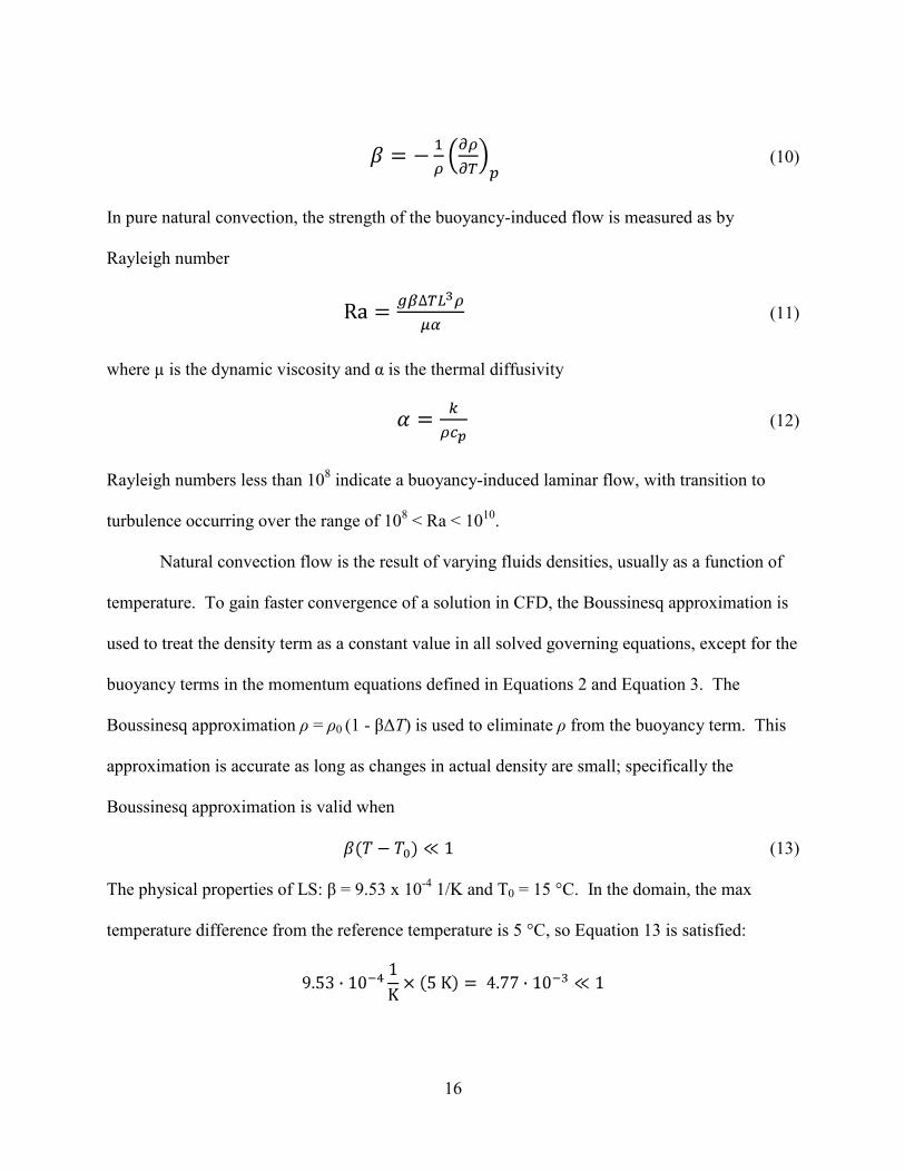
(10)
In pure natural convection, the strength of the buoyancy-induced flow is measured as by
Rayleigh number
(11)
where µ is the dynamic viscosity and α is the thermal diffusivity
(12)
Rayleigh numbers less than 108 indicate a buoyancy-induced laminar flow, with transition to
turbulence occurring over the range of 108 < Ra < 10
10.
Natural convection flow is the result of varying fluids densities, usually as a function of
temperature. To gain faster convergence of a solution in CFD, the Boussinesq approximation is
used to treat the density term as a constant value in all solved governing equations, except for the
buoyancy terms in the momentum equations defined in Equations 2 and Equation 3. The
Boussinesq approximation ρ = ρ0 (1 - βΔT) is used to eliminate ρ from the buoyancy term. This
approximation is accurate as long as changes in actual density are small; specifically the
Boussinesq approximation is valid when
(13)
The physical properties of LS: β = 9.53 x 10⁻⁴
1/K and T0 = 15 °C. In the domain, the max
temperature difference from the reference temperature is 5 °C, so Equation 13 is satisfied:

17
It is advised against using the Boussinesq model if there are large temperature gradients in the
domain (FLUENT User Guide Sec. 13.2.5).
2.2.5 Volume of Fluid (VOF) Theory
There are a few multiphase models available for use in FLUENT. The aim of this project
is to develop a multiphase flow regime consisting of a liquid-liquid stratified flow of two
immiscible fluids separated by a clearly-defined interface. The Volume of Fluid (VOF) model
theory is advised by FLUENT (User Guide Sec. 23.2.2) as a straightforward choice for stratified
flows. In the VOF model, a single set of momentum equations is shared by the fluids, and the
volume fraction of each of the fluids in each computational cell is tracked throughout the
domain.
The tracking of the interface between the phases is accomplished by the solution of a
continuity equation for the volume fraction of one or more of the phases. For the qth
phase,
FLUENT (User Guide Sec. 23.3.2) defines this equation of tracking the interface in the
following form
(14)
where is the mass transfer from phase q to phase p and is the mass transfer from phase
p to phase q. is the mass source term, but default by zero. When the VOF model is turned
on in FLUENT, a primary-phase is selected. The volume fraction equation will not be solved for
the primary phase; the primary phase volume fraction will be computed based on the following
constraint
(15)
18
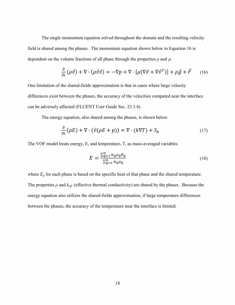
The single momentum equation solved throughout the domain and the resulting velocity
field is shared among the phases. The momentum equation shown below in Equation 16 is
dependent on the volume fractions of all phase through the properties ρ and µ.
(16)
One limitation of the shared-fields approximation is that in cases where large velocity
differences exist between the phases, the accuracy of the velocities computed near the interface
can be adversely affected (FLUENT User Guide Sec. 23.3.4).
The energy equation, also shared among the phases, is shown below.
(17)
The VOF model treats energy, E, and temperature, T, as mass-averaged variables
(18)
where Eq for each phase is based on the specific heat of that phase and the shared temperature.
The properties ρ and keff (effective thermal conductivity) are shared by the phases. Because the
energy equation also utilizes the shared-fields approximation, if large temperature differences
between the phases, the accuracy of the temperature near the interface is limited.

19
CHAPTER 3 CFD KAMLAND MODEL
3.1 Steps in Solving CFD Problem
Once the scope and details of a CFD project have been identified, there are a series of
steps FLUENT outlines that need to be completed to obtain in order to run a successful CFD
model. The steps are shown below.
1. Define the modeling goals.
2. Create the model geometry and grid.
3. Set up the solver and the physical models
4. Compute and monitor the solution.
5. Examine and save the results.
6. Consider revisions to the numerical or physical model parameters, if necessary.
3.2 The Modeling Goals
The purpose of this project is to obtain a CFD simulation of the KamLAND detector that
can first verify the validity of its results by producing realistic physical models of what is known
about the detector when it is not undergoing purification and what was observed during the past
purification programs. Second, the model needs to be robust in order to compute the month and
a half (or longer) purification process within a short time frame, preferably a week to coincide
with the rebooting of the servers that house the CFD software. Third, the model needs to be able
to be modified to try various methods of constraining the mixing that is observed: changing rates
of flow, varying the density to alter buoyancy forces, changing values of temperature of the
purified LS, etc.

20
3.3 Creating the Model Geometry
To create an accurate model of the KamLAND detector, the engineering drawings used in
the design and construction of KamLAND were provided and used as a basis for all dimensions
created. The schematic in Figure 3-1 displays all of the major parts of the detector: the liquid
scintillator (LS), the buffer oil (BO), the inner detector (ID), and the outer detector (OD) or
antiwater.
Figure 3-1. KamLAND detailed schematic.
Because of familiarity and ease of use, the commercial computer aided drawing (CAD)
software Pro/Engineer WildFire 4.0 (Pro/E) was used to create the complex solid geometry of
the concentric spheres curves, detector chimney, and the cylindrical outer detector. The solid
model created by Pro/E is shown in Figure 3-2.

21
Figure 3-2. KamLAND geometry created using Pro/E.
The next step is to use the Pro/E model and export the geometry, using the neutral data format
IGES that allows the digital exchange of data among CAD programs, to a grid generator. The
IGES file of was read into the grid generator program GAMBIT (Geometry and Mesh Building
Intelligent Toolkit). GAMBIT is a single, integrated preprocessor for CFD analysis (and can
also be used to create geometry, but is not as versatile as Pro/E). Due to inconsistencies between
the tolerances of the two CAD programs, the detector geometry had to be “healed” to get rid of
any hanging nodes or disconnected faces by using the Boolean operations of the program. The
“healed” geometry created by GAMBIT is shown in Figure 3-3. GAMBIT is then used to
simplify the geometry, mesh this simplified geometry, and assign boundary conditions.

22
Figure 3-3. GAMBIT geometry created from IGES file.
3.3.1 Simplyfying the KamLAND Geometry
The major parts of the KamLAND experiment are separated by walls whose thicknesses
are small with respect to the overall geometry. Meshing these walls with solid cells would lead
to high-aspect-ratio meshes and a significant increase in the total number of cells. Instead, these
solid walls are represented in GAMBIT by an edge that is assigned a “wall” boundary condition
used by FLUENT. FLUENT will solve a 1D conduction equation to compute the thermal
resistance offered by the wall, using the thickness and the thermal conductivity of the material
assigned to the wall.
Another simplification of the geometry shown in Figure 3-3 is to convert the 3D geometry into a
2D face for use in an axisymmetric, 2D model. This assumption was previously described in
Section 2.2.1 and greatly reduces the number of cells required for the CFD simulation. The
simplified geometry obtained is displayed in Figure 3-4. The geometry in Figure 3-4 was also

23
rotated so that the axis that the geometry will be revolved around lies along the x-axis. This is a
condition required by FLUENT when using the 2D axisymmetric model. The centers of the
spheres correspond to the origin of the system, with the positive z-axis pointing upward toward
the dome.
Figure 3-4. GAMBIT simplified geometry.
3.3.2 Meshing the KamLAND Geometry
The effect of resolution, smoothness, and cell shape of the mesh on the accuracy and
stability of the solution process is dependent on the flow field being simulated. The resolution of
the mesh describes the density of the nodes. A high resolution, or dense, mesh is required in the
domain where the fluid flow is a result of natural convection to resolve any large gradients
present. In regions of large gradients, it is important that the grid be fine enough to minimize the
change in flow variables from cell to cell. The smoothness of the mesh describes the changes in
sell volume between adjacent cells. Rapid changes results in large truncation errors, the

24
difference between the partial derivatives in the governing equations and their discrete
approximations. The cell shape (the skewness and aspect ratio) also has a significant impact on
the accuracy of the numerical solution. These three characteristics help quantify the quality of
the mesh and result in a warning if certain criteria are not met. Another important consideration
when meshing the geometry was the attachment of boundary layers along the edges in the
domains where flow occurs. Boundary layers provide high resolution by defining the spacing of
mesh node rows in regions immediately adjacent to edges and resolve the steep velocity
gradients near the wall due to no-slip wall conditions (the velocity is assumed to be zero at the
wall). For this project, since there were not any previous similar CFD simulation studies, there
was no way to estimate what resolution of the mesh was required.
In order to obtain this required resolution, mesh independence is required. This means
that increases in the resolution of the mesh, or increasing the density of the mesh, will not have
any effect on the calculated flow field solution, but will only increase the computational expense.
From earlier meshes created, there appeared to be a correlation between the size of the grid and
the mass continuity residuals. In one case with low mesh resolution, large mass continuity
residuals of 10+6
were observed and would not reduce below 10+3
. The convergence criterion for
the mass continuity residual is 10-3
. To better understand this correlation, a very simple
geometry was created to determine the resolution required. This geometry consisted of a sphere
and cylinder of the same dimensions as the KamLAND detector and modeled as 2D
axisymmetric. This simplified geometry is displayed in Figure 3-5. From the use of this
geometry in CFD simulations, with conditions comparable to that of the KamLAND experiment,
the mesh of the more complicated detector was developed. Trial and error resulted in the final

25
mesh used in the CFD simulation shown in Figure 3-6 (note that areas appear solid due to the
highly dense mesh).
Figure 3-5. Simple geometry of model used to test the grid resolution required.
Figure 3-6. Mesh used in KamLAND CFD simulation.

26
A close up of the boundary layers that were attached to the walls next to fluid flow, in the
domains of the LS, can be seen in Figure 3-7. The boundary layer captures the details of the
boundary flow at the wall. In the figure of the boundary layer, there are two transition rows from
the assignment of a transition patter of 4:2, where 4 is the mesh intervals in a given row and 2 is
the number of mesh intervals in the immediately preceding full row. This helps the smoothness
and skewness of the grid by controlling the transition of the quadrilateral cells of the boundary
layer to the triangular cells of the domain mesh.
Figure 3-7. Enlarged view of the boundary layer used on the walls of the LS domain.
In Figure 3-6, the bottom of the balloon was simplified into a horizontal edge equal in
dimension to the edge of the inlet located at the top detector. In earlier grids generated, the outlet
was treated as a small-diameter pipe, but this presented troubles in controlling the velocity scale
and produced highly skewed cells. The velocity scale of the inlet and outlet is determined by the

27
mass flow rate. The mass flow rate entering the detector is the same as the mass flow rate
leaving the detector, with mass flow rate defined as
(19)
Because the mass flow rates are the same, a large decrease in the area of the outlet, compared to
the area of the inlet, would result in a large increase of the velocity. With the outlet set to the
same area as the inlet, the velocity at the top of the detector inlet is of the same magnitude as the
velocity of the detector outlet at the bottom. To prevent the skewed cells produced, circled in
Figure 3-8, the outlet edge was moved to the bottom of the detector.
With these skewed cells removed and the velocity scale controlled, the time required for
the computation of each time step was greatly increased and the convergence of the solution was
faster as well.
Figure 3-8. Enlarged view of skewed cells in outlet pipe.

28
3.3.3 Description of the Grid
The grid consists of four major parts of the detector: the LS, BO, ID, and OD. Because
the direction of the flow field is not know and predicted to circulate inside of the domains,
triangular meshing was used in the fluid domains of the LS, BO, and ID. Quadrilateral meshing
was used in the OD, which is treated as a solid. Each domain was meshed using the Pave option,
which creates an unstructured grid of mesh elements and was found not to create any errors when
meshing the difficult curved geometry. The number of nodes and the number of elements of the
four major parts of the detector that make up the faces are listed in Table 3-1.
Before exporting the 2D mesh to FLUENT, it is easier to go ahead and set the boundary
conditions in GAMBIT and define the continuums. While exporting, GAMBIT will warn if
there are any highly skewed cells, as they can greatly affect the convergence of the solution or
the computational expense of the simulation.
Table 3-1. Details of the CFD mesh created in GAMBIT.
Face name Number of nodes Number of elements Boundary layer
Liquid scintillator 262 235 463 896 Yes
Buffer oil 221 645 316 278 Yes
Inner Detector 69 928 111 656 No
Outer Detector 15 178 1 468 No
Total 568 986 893 298 N/A

29
3.4 Pre-Processing of FLUENT
3.4.1 Reading in the Grid
It is during the pre-processing phase of the CFD that the physical models and solvers are
selected and supplied the necessary information. The first part of the pre-processing is reading in
the mesh to be used for the simulation. Because the model is axisymmetric, no nodes can lie
below the x-axis in FLUENT; as this would create a negative volume when FLUENT revolves
the model around the axis. Performing grid check will display if there are any nodes that violate
this. Again, because of the difference in the tolerances between GAMBIT and FLUENT, even
though no nodes lie below the grid in GAMBIT, during the export a few nodes will be listed as
below the axis. To easily correct this, translate the entire grid a small distance in the y-axis
direction, and then translate the grid that same distance in the reverse direction, and the
tolerances should be taken care of (note that this will not work if the double precision solver is
selected).
3.4.2 Defining the Material Properties and Boundary Conditions
For the KamLAND project, the physical properties for all the major materials within the
detector are needed to perform an accurate simulation and are provided in Appendix C. It is
important to note that, to be able to model natural convection in the flow, the density for liquids
used in the simulation must be set to either Boussinesq or be a function of temperature. The
physical parameters of every boundary condition, assigned in GAMBIT and provided in
Appendix D, also need to be supplied. The center of the balloon was set to an “axis” boundary
condition as required for an axisymmetric case. The LS inlet of the detector, located at the top of
the chimney, was set to “mass-flow inlet” with a mass flow rate of 1.1 m3 / hour, recorded over
the course of the first campaign as displayed in Figure 3-9. It should be noted that for 2D

30
axisymmetric problems, the mass flow rate assigned to the boundary condition is the flow rate
through the entire (2π-radian) domain, not through a 1-radian slice.
Figure 3-9. Density and mass flow rate of LS over the course of the first purification process.
To help the simulation along computationally by avoiding reverse flow on the edge
where the LS is withdrawn, this outlet located at the bottom of the balloon was also set to a
boundary condition of “mass-flow inlet,” with the same mass flow rate as the inlet. The major
difference between the two: the axial component of the outlet was set to -1 to induce outflow.
There were other boundary conditions that could be set for the inlet and outlet for the simulation.
For the LS inlet, a “velocity inlet” could also have been specified. For the LS outlet, the edge
could have been set as an “outflow” boundary condition, but this resulted in reverse flow on the
edge and is also not recommended for use with multiphase models. The majority of the

31
remaining edges were set to “wall” boundary conditions, with thickness and material assigned.
Details of the boundary conditions are listed in Appendix D.
The outer detector, or antiwater, posed a unique problem to the simulation. Outside of
the cylindrical wall of the OD, the solid rock of the mine acts as a heat sink. There were not any
measured temperature values of the OD’s walls to assign to the boundary condition. But, there
were temperature measurements made of the water contained in the OD at various elevation
levels, displayed in Figure 3-10. It can be observed that the bottom of the OD was consistently
at 10° C, so this constant temperature was set as the boundary condition for the bottom edge of
the OD.
Figure 3-10. Plots of temperature versus time of four elevation levels within the OD.

32
But the cylindrical wall of the OD was not a constant temperature as the elevation increased.
Since it was observed that the temperatures stayed fairly constant over time, each elevation was
assigned a constant temperature measurement. A polynomial function was then fitted to the
values for the elevations and their respective temperatures as displayed in Figure 3-11.
Figure 3-11. Polynomial trendline of OD temperature versus distance along z-axis.
This polynomial function was compiled into a user defined function (UDF), see Appendix E, to
specify this temperature profile along the cylindrical wall of the OD. The temperature in the
dome above detector was measured to be an average of 19 °C, so this was set as the constant
temperature for the edge representing the wall between the OD and dome.
Another unique problem was the presence of the 1,911 photomultiplier tubes (PMTs)
located on the stainless steel wall of the inner detector, behind the acrylic glass that separates the
y = 2.825E-04x4 + 2.732E-03x3 - 1.462E-03x2 + 1.381E-01x + 1.200E+01
10.0
11.0
12.0
13.0
14.0
15.0
16.0
17.0
18.0
19.0
20.0
Tem
pe
ratu
re (
oC
)
Z-axis (meters)

33
buffer oil from the inner detector. The detected power of output of each PMT was estimated to
be 0.4 Watts / PMT. Using the following formula
(19)
a volumetric heat generation rate for the “wall” boundary condition representing the steel sphere
of the ID was calculated to apply these heat sources to the model.
The continuum in each of the domains was assigned the appropriate material. In the OD,
water was set as the material. The ID and BO domains contain a non-scintillating, ultra clear
mineral oil and the domain of the LS detector contains the liquid scintillator. These material
properties were created in the FLUEN materials database and are listed in Appendix C. To
further simplify the program and from calculation run errors, it was decided to set the OD, ID,
and BO domains as solids with the same thermal conductivity as their liquid counterparts. This
assumption was made due to the stable temperature profile that had been measured over the
course of the KamLAND project in each of these regions. This greatly helped computational
time, as only the flow field for the LS needed to be calculated.
3.4.3 Enabling the Desired Physical Models
With all of the boundary conditions set, the next part of the pre-processing of CFD
simulation is to set the physical models that will be calculated. In the operating conditions, the
value for gravity is entered in the desired direction and a reference temperature is set for the
Boussinesq parameter. The VOF simulation is the best choice for stratified and liquid-liquid
flows, so the necessary parameters are selected or entered, such as the selection of the primary-
phase (for this simulation, the unpurified LS is the best choice) and selection of the VOF implicit
scheme due to the presence of gravity. When large body forces (e.g., gravity) exist in multiphase

34
flow, the body force and pressure gradient in the momentum equation are almost in equilibrium,
with the contributions of convective and viscous terms small in comparison. Segregated
algorithms converge poorly unless partial equilibrium of pressure gradient and body forces is
taken into account (FLUENT User Guide 23.9.4).
3.4.5 Initializing the Solution
With the VOF and natural convection physical models enabled, nothing was changed in
the solver except to make sure the 2d axisymmetric was enabled. The next step was to initialize
the solution, or set values to the grid that served as a starting point for the calculations. The
temperature at the center of the detector is roughly 12.5 °C, so this was chosen as a good
estimate for the temperature initialization value. For the KamLAND project, measurements have
confirmed that during non-purification campaigns there was almost no flow, with velocity
magnitudes around 10-8
m/s, so values of zero are set for the radial and axial velocities’
initialization values.
Because there was almost no flow present before the first purification process, the energy
and flow equations could be decoupled; the energy equation was only solved to obtain a
distributed temperature profile to act as an initial temperature profile for the transient
calculations involving multiphase flow. This essentially turned the model into a heat transfer
problem with conduction only. This method was found to obtained a temperature profile along
the z-axis and inside of the detector that was very close to measurements taken along the z-axis
and in the detector. A comparison of the temperature distribution measured in the KamLAND
experiment before the purification process and the initial temperature distribution calculated
before transient flow is displayed in Figure 3-12 and Figure 3-13, respectively.
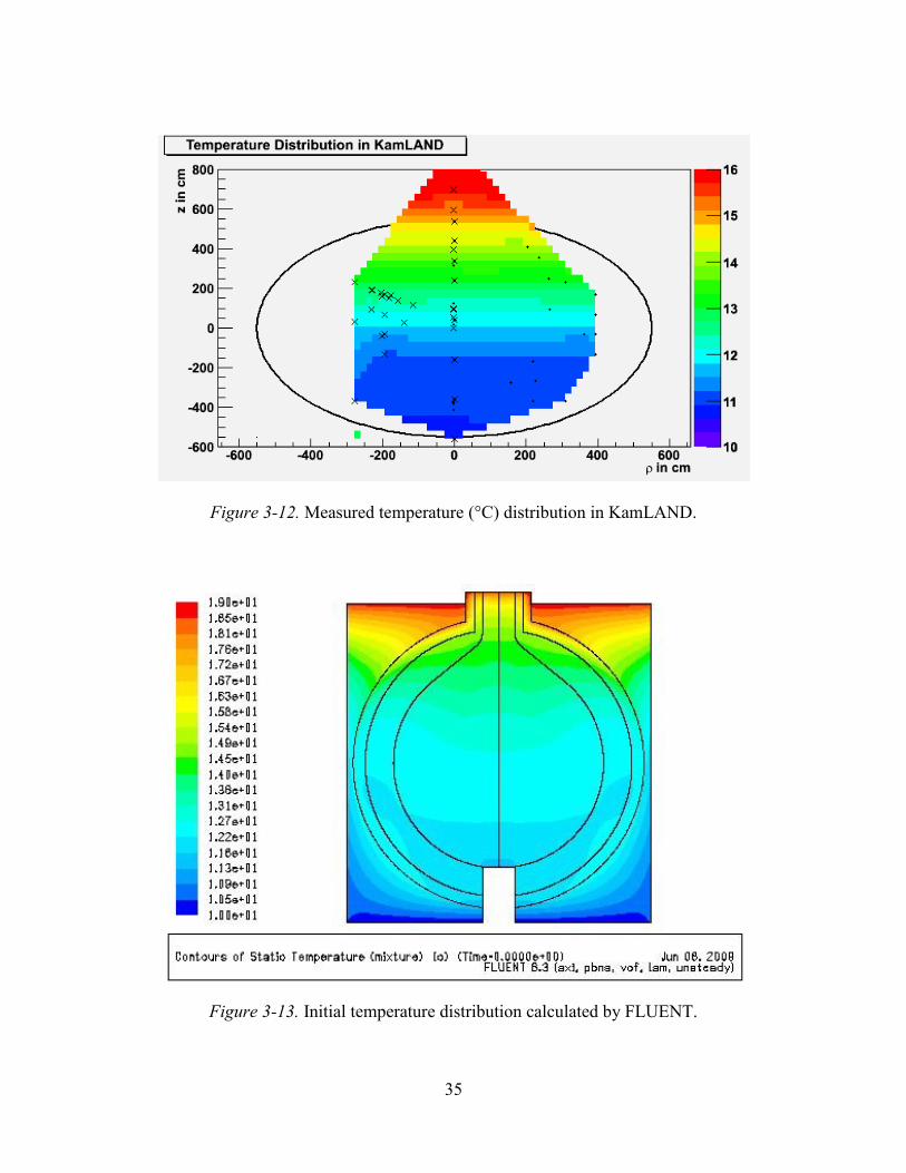
35
Figure 3-12. Measured temperature (°C) distribution in KamLAND.
Figure 3-13. Initial temperature distribution calculated by FLUENT.

36
3.4.6 Selecting the Solution Controls
With the distributed temperature flow field solved, the next step was to couple the energy
and flow equations and solve the simulation as a steady state problem. But with the more
complex problem of flow and energy solved for, the multiple parameters in the solution controls
needed to be assessed to obtain the right selection of the pressure-velocity coupling scheme, the
appropriate discretization scheme, and the values for the under-relaxation factors of the variables
solved: pressure, density, body forces, momentum, and energy. Because of the nonlinearity of
the equation set being solved by FLUENT, it is necessary to control the change of φ, or the
variable being solved for. This is typically achieved by under-relaxation of variables (also
referred to as explicit relaxation), which reduces the change of φ produced during the iteration.
In a simple form, the new value of the variable φ within a cell depends upon the old value, φold,
the computed change in φ, Δ φ, and the under relaxation factor, α, displayed below in
(20)
The FLUENT User’s Guide provided some guidance on these choices, but most CFD
problems are unique and there is no definite right answer about what choice is the best without
selecting it and running the simulation. This was where closely monitoring the residuals
(continuity, x and y-velocities, and energy) of the simulation during the iterations became
important to observe the progress of the solution. Residuals (FLUENT User Guide 25.18) are a
way to monitor the convergence of the solution; the solution is considered converged when these
residuals have decreased to their defined criteria, usually dropping several orders of magnitude.
With the default solution controls selected, the steady state simulations with flow and
energy coupled was slow to converge and produced unrealistic results. This can be seen in initial

37
temperature distribution seen in Figure 3-14, obtained as described in section 3.4.5, and a
converged steady state solution with flow and energy coupled displayed in Figure 3-15.
Instead of a stratified thermal distribution that had been observed, the domains containing
flow experienced thermal mixing that resulted in a mostly homogenous temperature profile
throughout.
Figure 3-14. Temperature distribution of solution with only the energy equation solved.
Figure 3-15. Temperature distribution with energy and flow equations coupled.

38
It was not understood what was creating the thermal mixing effect that should not have
been present. As was the case for developing the necessary resolution for the grid, the simplified
geometry in Figure 3-5 was used to model a simpler CFD simulation of natural convection, with
a similar temperature profile and fluid conditions as that of the physical KamLAND experiment.
It was also during this simpler simulation that the UDF temperature profile was implemented to
more accurately reflect the measured temperature values of the OD. In the simplified simulation,
the domain of the cylinder was treated as a solid with the thermal properties of water and the
domain of the sphere was set as a liquid containing the LS. With only energy solved for, a
distributed temperature profile was obtained and is displayed in Figure 3-16. With the default
controls and flow and energy coupled, again, the converged steady state solution experienced
homogenous thermal mixing but with the impossible event of viscous heating in the sphere that
resulted in a temperature greater than the maximum temperature present. This is shown in
Figure 3-17.
Figure 3-16. Temperature distribution in simple CFD model with only energy solved.

39
Figure 3-17. Temperature distribution in simple CFD model with energy and flow solved.
Upon further research and investigation, it was found that the reduction in the under-
relaxation factor for the momentum variable is necessary to prevent unrealistic results and
divergence. Because the velocity magnitudes are low, on the order of 10-3
to 10-5
, the under-
relaxation factors help impedes the amount of change in the momentum equations during
iterations, helping convergence. For a natural convection problem, where the energy field
impacts the fluid flow (via temperature dependent properties or buoyancy), a lower value for the
under-relaxation factor, typically in the range of 0.8 to 1.0, was also found to be helpful. The use
of the simple CFD model of natural convection helped to understand how the under-relaxation
factors contributed a major role in obtaining a stabile converged solution.
With the knowledge obtained concerning the discretization schemes and the under-
relaxation factors, the next step was to solve a transient, multiphase solution of the purification
process using the KamLAND geometry. FLUENT provides some guidance on solving a
40
multiphase system that is encountering some stability or convergence problems. If a time-
dependent problem is being solved, and patched fields are used for the initial conditions, it is
recommended to perform a few iterations with a small time step, at least an order of magnitude
smaller than the characteristic time of the flow. And then increase the size of the time step after
performing a few time steps.
3.5 Computing the Solution of FLUENT
The purification program at KamLAND lasted approximately a month and a half. While
computing and monitoring the solution, this was kept in mind in order to make sure the time
steps were large enough to account for the large amount of time that needed to be computed
while keeping the solution stable. To help facilitate the processing of this large amount of time
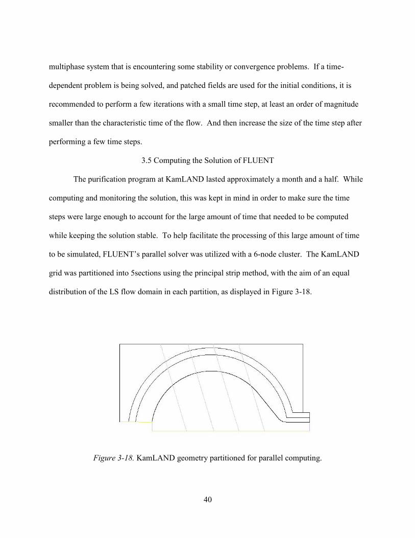
to be simulated, FLUENT’s parallel solver was utilized with a 6-node cluster. The KamLAND
grid was partitioned into 5sections using the principal strip method, with the aim of an equal
distribution of the LS flow domain in each partition, as displayed in Figure 3-18.
Figure 3-18. KamLAND geometry partitioned for parallel computing.

41
The time steps were steadily increased (from 0.1 seconds to 120 seconds) until an
optimal time step was observed. Larger time steps would sometimes require longer
computational effort and more time steps than that of a smaller time step calculated for the same
span of time. Each time step should take approximately 5-15 iterations to converge for an
efficient transient solution. The optimal time step of 120 seconds for the simulation resulted in
twelve simulated days for a day of computation, making it possible to simulate approximately
two months in a week of computation. For a stable, transient CFD simulation’s residuals should
appear to a saw-tooth pattern. This is seen the KamLAND CFD simulation’s scaled residuals
plot in Figure 3-19. See Appendix F for a work sheet maintained while the simulation was
running.
Figure 3-19. Scaled residuals plot of the KamLAND CFD simulation.

42
3.6 Post-Processing the Results of FLUENT
To be able to review data obtained in an experiment is very important to see if the goals
of the experiment have been met. When a case file (or .cas file) of a simulation is written, it
contains the mesh, material properties, boundary conditions, and the settings for the solver. This
makes it easy to track changes made. To record the variables solved for at each node, a data (or
.dat) file is created. Because much of this CFD simulation involved continuous, unmonitored
computing time, FLUENT was set to automatically create a .dat file at specified time step
intervals that amounted to four hours of flow time calculation. From this data file any of the
contours can be readily accessible as well as any fluxes that may have been computed.

43
CHAPTER 4 RESULTS AND DISCUSSION
The following figures from Figure 4-1 to Figure 4-10 are the results from the KamLAND
CFD simulation that was ran as KamLAND_2Dv10vof.cas and the details of this simulation is
given in Appendix E. Figure 4-1 through Figure 4-9 display eight weeks of which purification of
the LS was occurring. Figure 4-10 displays a week after purification was stopped and now flow
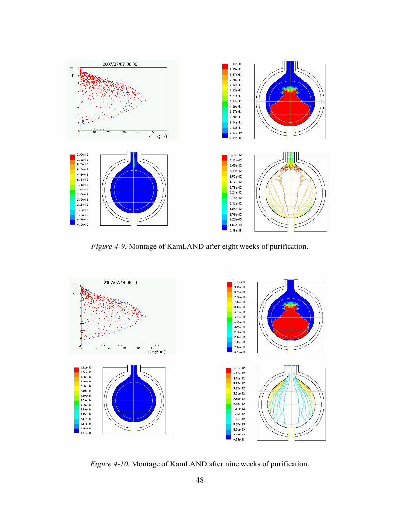
entered or left the LS detector. The montage figures below each contain four figures:
KamLAND 222
Rn tracking, see Appendix B (top left), CFD contours of volume fraction
[unpurified] (top right), CFD contours of velocity magnitude [m/s] (bottom left), and CFD
contours of stream function [kg/s] (bottom right).
The top two figures in the montage cannot be compared directly, but the figure on the left
serves as a reference. This is due to the fiducial volumes cuts used to normalize the 222
Rn plot,
as this is seen in the units of the horizontal axis of the plot. The three horizontal lines that appear
in the FLUENT images of Figure 4-1 to Figure 4-10serve as referential marking. The middle
line lies at the center of the detector on the z-axis, and the lines above and below are each spaced
3.5 meters from this center. The montage in Figure 4-11 displays the temperature contours in
chronological order, from left to right, top to bottom.

44
Figure 4-1. Montage of KamLAND after one day of purification.
Figure 4-2. Montage of KamLAND after one week of purification.

45
Figure 4-3. Montage of KamLAND after two weeks of purification.
Figure 4-4. Montage of KamLAND after three weeks of purification.

46
Figure 4-5. Montage of KamLAND after four weeks of purification.
Figure 4-6. Montage of KamLAND after five weeks of purification.

47
Figure 4-7. Montage of KamLAND after six weeks of purification.
Figure 4-8. Montage of KamLAND after seven weeks of purification.
48
Figure 4-9. Montage of KamLAND after eight weeks of purification.
Figure 4-10. Montage of KamLAND after nine weeks of purification.

49
Figure 4-11. Montage of KamLAND CFD simulation temperature profile.
The montage in Figure 4-1 displays the CFD simulation after one day of purification.
The newly purified LS has already traversed the chimney and is entering the spherical balloon.
At this point, a clear interface is visible. Of concern is the high velocity magnitudes displayed in
the chimney.
After a week of purification as seen in Figure 4-2, this slightly level interface between the
old and new LS is present in both the CFD and 222
Rn tracking. The maximum velocity
magnitude has decreased by an order of 103 after the simulation has been running for an
extended period of time. This behavior was observed in earlier simulations. The dark blue in

50
Figure 4-1 indicates velocities flow below 10-5
meters per second which is within the range of
observed values.
After two weeks of the multiphase purification CFD simulation displayed in Figure 4-3,
the VOF contours contain a noticeable angle slope from the axis towards the outside. This is not
seen the the 222
Rn tracking, but this process has trouble seeing events that lie close along the
surface of the balloon. It is a prediction that the purified LS has started to travel along the
surface of the balloon as indication by the stream lines of the stream function contour plot.
In Figure 4-4, the VOF contours plot displays a swelling that runs along the axis of the
model. It has been noted on observations of the purification process, that at this 3.5 meter mark,
there is noticeable mixing and that the expected level stratification interface starts to disappear in
the 222
Rn model. In the top left figure, the purified LS appears to be strongly following along the
circular path of the edge of the balloon. Again, in the VOF contour plot in Figure 4-5, there is
not a level interface as predicted by the 222
Rn tracking plot.
From the five week mark, displayed in Figure 4-6, to the end of the purification,
displayed in Figure 4-9, it is interesting to note that in the plots of the 222
Rn event tracking, the
cluster of dots no longer follows the predicted line of volumetric filling and as time lapses, are
noticeably absent from the bottom of the LS detector. This compelling case demonstrates that
the 222
Rn events are occurring less than what is expected because the flow is moving along the
balloon in the detector during this purification process. There is clearly some kind of a mixing
boundary occurring around 3.5 meters above the center that prevents the longitudinal movement
of the purified LS along the z-axis and instead reroutes it towards the boundary of the balloon.

51
One complete volume (1 kton) of the liquid scintillator inside the balloon has been
purified and replaced back into the balloon as shown in Figure 4-10. The majority of the
measured 222
Rn events are still in the upper region of the scintillator, while the region from 3.5 to
-3.5 meters remained unpurified.
The spacial distribution plot shown Figure 4-12 provides some backup evidence that the
swelling occurring in the CFD simulation phase contour plots are actual physical representations
of the purification system. The plot was taken roughly between the sixth and seventh week of
purification. Because the fiducial volume cut has been removed, this plot is a closer reference to
the distribution of the purified LS with respect to radial coordinates. In the plot, there is a
noticeable absence of events in the center of the detector; this absence is clearly visible in the
CFD images, Figure 4-6 and Figure 4-7, that represent the estimated time of Figure 4-12.
Figure 4-12. Spacial distribution of BiPo events with the fiducial volume cut removed.

52
CHAPTER 5 CONCLUSIONS
Working on a complex computational fluid dynamics (CFD) simulation is a learning
process of trial and error to determine what assumptions, physical models, and solution
parameters are required to obtain an accurate representation of the problem being modeled. The
modeling of the purification process of the KamLAND experiment posed a unique challenge in
creating a CFD simulation to model the relatively small velocity magnitudes due to natural
convection and the fluid interface between the purified and unpurified liquid scintillator (LS) in a
large spherical domain over the time span of two months. Another challenge of the problem,
because of physical constraints of the KamLAND experiment, the only empirical data
concerning the flow and interaction between the purified and unpurified LS was from the method
of tracking 222
Rn daughters. The plots obtained from this method could not be compared directly
to the CFD simulated plots of interaction between these fluids, but served more as a reference.
For the CFD simulation, the geometry and meshing of the model played important roles
in the accuracy and converging of solutions of the model. Modifications were made to the
geometry so that a 2D axisymmetric model could be applied to simplify the 3D geometry. Also,
most of the thin walls, in comparison to the dimensions of the overall geometry, were modeled as
edges with an assigned wall thickness for 1D conduction heat transfer calculations. These
modifications helped greatly reduce the computational resources required. For the mesh of the
model, boundary layers, consisting of highly dense rows of cells along a wall, were attached to
edges in the domain to capture the details of the fluid flow at the walls. A high degree of
resolution of the mesh in the fluid domain was determined to be required to be able to accurately
53
portray the effect of natural convection. Without this high resolution of the mesh, convergence
of the solution of the simulation was unobtainable due to large mass continuity residuals.
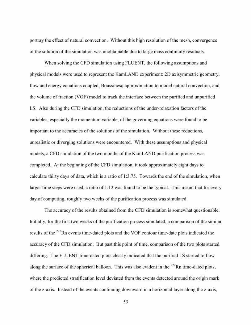
When solving the CFD simulation using FLUENT, the following assumptions and
physical models were used to represent the KamLAND experiment: 2D axisymmetric geometry,
flow and energy equations coupled, Boussinesq approximation to model natural convection, and
the volume of fraction (VOF) model to track the interface between the purified and unpurified
LS. Also during the CFD simulation, the reductions of the under-relaxation factors of the
variables, especially the momentum variable, of the governing equations were found to be
important to the accuracies of the solutions of the simulation. Without these reductions,
unrealistic or diverging solutions were encountered. With these assumptions and physical
models, a CFD simulation of the two months of the KamLAND purification process was
completed. At the beginning of the CFD simulation, it took approximately eight days to
calculate thirty days of data, which is a ratio of 1:3.75. Towards the end of the simulation, when
larger time steps were used, a ratio of 1:12 was found to be the typical. This meant that for every
day of computing, roughly two weeks of the purification process was simulated.
The accuracy of the results obtained from the CFD simulation is somewhat questionable.
Initially, for the first two weeks of the purification process simulated, a comparison of the similar
results of the 222
Rn events time-dated plots and the VOF contour time-date plots indicated the
accuracy of the CFD simulation. But past this point of time, comparison of the two plots started
differing. The FLUENT time-dated plots clearly indicated that the purified LS started to flow
along the surface of the spherical balloon. This was also evident in the 222
Rn time-dated plots,
where the predicted stratification level deviated from the events detected around the origin mark
of the z-axis. Instead of the events continuing downward in a horizontal layer along the z-axis,

54
past a horizontal interface at the origin, events were no longer detected in the middle of the
domain, but along the balloon’s surface. Though the main difference observed in the time-dated
plots comparison was the sloping from the z-axis that occurred along the two liquid’s interface in
the FLUENT plot of the VOF contours. The top of the slope was approximately 3.5 meters
above the origin along the z-axis and seemed to indicate a region of the unpurified LS that acted
as a barrier that resisted the purified LS and redirected it outward. Another possible cause of this
outward sloping that was suggested was the spherical shape of the balloon. There are not any
previous studies to be found on the possible effects this shape has on the fluid flow within it.
From discussions with the KamLAND Collaboration, it was noted that below this same positive
elevation level of 3.5 meters above the origin there appeared to be a spherical region of fluid that
the purified LS was not able to progress any further. This was not seen in the 222
Rn events plots,
but possibly evident in BiPo events plots with the fiducial volume cut removed. The BiPo events
plot showed events densely clustered along the surface of the balloon and with an outward slope
in the interface. From these discussions, it was assumed that the CFD simulation is accurate
enough to serve as a representation of the purification process of the KamLAND experiment
The CFD simulation will be used to test proposed improvements to the purification
process for future purification programs of KamLAND. The proposed improvements, with the
aim of obtaining a horizontally stratified interface and minimizing natural convection, involve
varying the physical properties, such as the density, and/or the temperature of the purified LS
entering the detector. It is hoped that enough CFD simulations with these improvements can be
completed before the next purification program to act as guides for the implementation of a more
efficient purification process that will be able to meet the reduction goals necessary for the
objectives of the KamLAND experiment.

55
REFERENCES
Anderson, J. D., Jr. (1995). Computational fluid dynamics: the basics with applications. New
York: McGraw-Hill, Inc.
ANSYS® FLUENT (Version 6.3). FLUENT 6.3 User’s Guide [Software manual].
Batchelor, G. K. (1967). An introduction to fluid dynamics. Cambridge, England: Cambridge
University Press
Bejan, A. (2004). Convection heat transfer (3rd ed.). New Jersey: John Wiley and Sons
Campbell, C. E. (2002). Natural convection in a rectangular enclosure with a pipe attached. M.S.
dissertation, University of Massachusetts Lowell, United States -- Massachusetts.
Retrieved June 8, 2009, from Dissertations & Theses: Full Text database. (Publication
No. AAT 1409915).
Catton, I. (1978). Natural convection in enclosures. Proceedings of the sixth international heat
transfer conference, Toronto (Vol. 6). Washington, D.C.: Hemisphere Publishing Corp.
Ede, A. J. (1967). Advances in free convection. Advances in heat transfer (Vol. 4). New York:
Academic Press
Freitas, C. J. (Ed.). (1993). The CFD triathlon: Three laminar flow simulations by commercial
CFD codes. Presented at the Fluids Engineering Conference, Washington, D.C. (FED-
Vol. 160). New York: ASME, United Engineering Center
Gebhart, B. (1979). Buoyancy induced fluid motions characteristic of applications in technology.
The 1978 Freeman Scholar Lecture, J. Fluid Engr (Vol. 101).
Hoogendorn, C. J. (1986). Natural convection in enclosures. Proceedings of eighth international
heat transfer conference, San Francisco (Vol. 1). Washington, D.C.: Hemisphere
Publishing Corp.
Iwamoto, T. (2003). Measurement of reactor anti-neutrino disappearance in KamLAND. Ph.D.
dissertation, Tohoku University, Japan. Retrieved June 6, 2009, from
http://kamland.lbl.gov/Dissertations/

56
Jing, X., Xiao, J, & Zhou, Z. (2005) Multi-dimensional simulation of hydrogen mixing and
transport in the containment using CFD codes. Presented at the 18th
international
conference on structural mechanics in reactor technology, Beijing, China (SMiRT 18-
P02-8). Retrieved February 5, 2009, from https://www.iasmirt.org/iasmirt-2/SMiRT18/
Kamioka Liquid Scintillator Antineutrino Detector. (2009, May 19). In Wikipedia, The Free
Encyclopedia. Retrieved May 19, 2009, from
http://en.wikipedia.org/w/index.php?title=Kamioka_Liquid_Scintillator_Antineutrino_De
tector&oldid=290888735
KamLAND Collaboration (n.d.) Retrieved May 19,2009, from http://kamland.lbl.gov/
Kishimoto, Y. (2007). KamLAND status for solar neutrino phase. J. Phys.: Conf. Ser. 120. doi:
10.1088/1742-6596/120/5/052010
Ostrach, S. (1964). Laminar flows with body forces: High speed aerodynamics and jet
propulsion. In F. K. Moore (Ed.), Theory of laminar flows (Vol. 4). Princeton University
Press
Ostrach, S. (1972). Natural convection in enclosures. Advances in heat transfer (Vol. 8). New
York: Academic Press
Ostrach, S. (1982). Natural convection heat transfer in cavities and cells. Proceedings of seventh
international heat transfer conference, Munich (Vol. 1). Washington, D.C.: Hemisphere
Publishing Corp.
O'Malley, C. (2003). Computational fluid dynamics model of natural convection airflow inside a
commercial 30" wall oven using FLUENT. M.S.M.E. dissertation, University of
Louisville, United States -- Kentucky. Retrieved June 8, 2009, from Dissertations &
Theses: Full Text database. (Publication No. AAT 1459527).
Stein, E., de Borst, R., Hughes, T. J. R. (Eds.). (2004). Encyclopedia of Computational
Mechanics (Vol. 3: Fluids). West Sussex, England: John Wiley & Sons, Ltd.
Suzuki, A. et al. (2005). Results from KamLAND reactor neutrino detection. Phys. Scr. T121,
33-38. doi: 10.1088/0031-8949/2005/T121/004
Tajima, O. (2003). Measurement of electron anti-neutrino oscillation parameters with a large
volume liquid scintillator detector, KamLAND. Phd. dissertation, Tohoku University,
Japan. Retrieved June 6, 2009, from http://kamland.lbl.gov/Dissertations/
Yao, H. (1999). Studies of natural convection in enclosures using the finite volume method.
Ph.D. dissertation, York University (Canada), Canada. Retrieved June 6, 2009, from
Dissertations & Theses: Full Text database. (Publication No. AAT NQ42781)
Holman, J.P. (2002) Heat transfer (9th ed.). New York: McGraw-Hill
A-1
APPENDIX A KAMLAND COLLABORATION
KamLAND collaboration
K. Eguchi,1 S. Enomoto,1 K. Furuno,1 J. Goldman,1 H. Hanada,1 H. Ikeda,1 K. Ikeda,1 K. Inoue,1
K. Ishihara,1W. Itoh,1 T. Iwamoto,1 T. Kawaguchi,1 T. Kawashima,1 H. Kinoshita,1 Y. Kishimoto,1
M. Koga,1 Y. Koseki,1 T. Maeda,1 T. Mitsui,1 M. Motoki,1 K. Nakajima,1 M. Nakajima,1
T. Nakajima,1 H. Ogawa,1 K. Owada,1 T. Sakabe,1 I. Shimizu,1 J. Shirai,1 F. Suekane,1 A. Suzuki,1
K. Tada,1 O. Tajima,1 T. Takayama,1 K. Tamae,1 H. Watanabe,1 J. Busenitz,2 Z. Djurcic,2
K. McKinny,2 D-M. Mei,2 A. Piepke,2 E. Yakushev,2 B.E. Berger,3 Y.D. Chan,3 M.P. Decowski,3
D.A. Dwyer,3 S.J. Freedman,3 Y. Fu,3 B.K. Fujikawa,3 K.M. Heeger,3 K.T. Lesko,3 K.-B. Luk,3
H. Murayama,3 D.R. Nygren,3 C.E. Okada,3 A.W. Poon,3 H.M. Steiner,3 L.A. Winslow,3
G.A. Horton-Smith,4 R.D. McKeown,4 J. Ritter,4 B. Tipton,4 P. Vogel,4 C.E. Lane,5 T. Miletic,5
P. Gorham,6 G. Guillian,6 J. Learned,6 J. Maricic,6 S. Matsuno,6 S. Pakvasa,6 S. Dazeley,7
S. Hatakeyama,7 M. Murakami,7 R.C. Svoboda,7 B.D. Dieterle,8 M. DiMauro,8 J. Detwiler,9
G. Gratta,9 K. Ishii,9 N. Tolich,9 Y. Uchida,9 M. Batygov,10 W. Bugg,10 H. Cohn,10 Y. Efremenko,10
Y. Kamyshkov,10 A. Kozlov,10 Y. Nakamura10 C.R. Gould,11 H.J. Karwowski,11 D.H. Markoff,11
J.A. Messimore,11 K. Nakamura,11 R.M. Rohm,11 W. Tornow,11 A.R. Young,11 andY-F.Wang12
1 Research Center for Neutrino Science, Tohoku University, Sendai 980-8578, Japan
2 Department of Physics and Astronomy, University of Alabama, Alabama 35487, USA
3 Physics Department, University of California at Berkeley and Lawrence Berkeley National
Laboratory, Berkeley, California 94720, USA
4 W. K. Kellogg Radiation Laboratory, California Institute of Technology, Pasadena, California
91125, USA
5 Physics Department, Drexel University, Philadelphia, Pennsylvania 19104, USA
6 Department of Physics and Astronomy, University of Hawaii at Manoa, Honolulu, Hawaii
96822, USA
7 Department of Physics and Astronomy, Louisiana State University, Louisiana 70803, USA
8 Physics Department, University of New Mexico, Albuquerque New Mexico 87131, USA
9 Physics Department, Stanford University, California 94305, USA
10 Physics Department, University of Tennessee, Tennessee 37996, USA
11 Triangle Universities Nuclear Laboratory, Durham, NC 27708, USA and
Physics Departments at Duke University, North Carolina State University, and the University
of North Carolina at Chapel Hill
12 Institute of High Energy Physics, Beijing 100039, People’s Republic of China

B-1
APPENDIX B METHOD OF TRACKING 222
RN DAUGHTERS
Note: This explanation of the tracking of 222
Rn daughters to determine the location of purified LS
was provided by Chris Grant, a member of the Physics Department of the University of
Alabama, which is a part of the KamLAND Collaboration.
The gaseous 222
Rn isotope appears naturally within our atmosphere and acts as a
radioactive background in KamLAND (it eventually decays into 210
Pb which has ~22 year half
life; 210
Pb will then decay into 210
Bi and 210
Po, both of which will hide the solar neutrino signal
we want to observe). 222
Rn can enter KamLAND scintillator through tiny leaks in the pipes
which carry the purified scintillator from the distillation system back into the detector.
Extensive leak testing is conducted to minimize the amount of 222
Rn that sneaks into the
purified scintillator, but there is always a tiny amount that gets into the detector. As long as the
amount of 222
Rn that sneaks into the purified scintillator is less than 1 mBq in activity, our
purification will not be ruined. (Note:1 Bq = 1 decay/second, and 1 mBq = 1 decay/1000
seconds; Bq means “Bequerel”). The amount of 222
Rn entering the detector is monitored as it is
being filled during purification to make sure there is not recontamination the scintillator.
KamLAND is an extremely sensitive particle detector, so observing only a few atoms of
222Rn in the 1-kton detector is possible (the time, position and energy of all events in the detector
are collected). Monitoring 222
Rn contamination also provides a picture of the separation between
purified and un-purified scintillator. 222
Rn has a 3.8 day half life, so it will have already

B-2
decayed away completely in the un-purified scintillator. It will be observable in the purified
scintillator for roughly 1 month before it has completely decayed away. To measure 222
Rn, the
decay scheme is shown below in Figure B-1.
Figure B-1. Decay scheme for 222
Rn.
The half-lives are shown in brackets and the decay type is given next to the arrows. We can
measure 222
Rn by measuring the activity of its daughters, 214
Bi and 214
Po. 210
Pb will feed 210
Bi
and 210
Po for a long time, which is bad for KamLAND. All the daughters after 222
Rn (but before
210Pb) have very short half-lives compared to 3.8 day half-life of
222Rn. This means that the
daughters, 214
Bi and 214
Po, will have the same activity as 222
Rn (this is known as secular
equilibrium).
Why use 214
Bi and 214
Po? It can be seen that if a 214
Bi atom decays into 214
Po, the 214
Po
will decay, on average, within 0.164 milliseconds (very fast!). It is highly improbable that any
other events will occur in such a short time window after a 214
Bi decay. This means we can look
at all the physics events in the KamLAND data and only choose events that “coincide” with this
very fast decay of 214
Po after 214
Bi.
To choose 214
Bi events, an energy selection cut is made in the data (since 214
Bi decays
with a certain energy that follows a known statistical distribution): –0.45 < Eprompt < 3.00 MeV

B-3
(214
Bi is the “prompt” event). A time window is opened in the data (~1.2 milliseconds) after this
“prompt” 214Bi event and the possible 214Po events are collected using another energy selection
cut: –0.45 < Edelay < 0.80 MeV (214
Po is the “delay” event). Event pairs are also required to be no
more than 120 cm apart from one another. Pairs of events that satisfy the conditions above are
collected. Histograms of the data can be seen below in Figure B-2.
Figure B-2. Pairs of events that satisfy energy selection cut for 214
Bi-214
Po events.
Monte Carlo simulations of 214
Bi-214
Po events in the KamLAND detector agree very well with
the data shown in Figure B-2, confirming the event selection. Each one of these 214
Bi-214
Po pair

B-4
of events in the data set corresponds to a single 222
Rn decay. Counting the number of 214
Bi-214
Po
pairs over a period of time will tell us the 222
Rn activity (number of decays per second). This can
then be used to plot the position of these pairs of events in the detector as shown in Figure B-3.
Figure B-3. Dots representing 214
Bi-214
Po event pair from the decay of 222
Rn in the detector.

C-1
APPENDIX C MATERIALS PARAMETERS
Liquid Scintillator @ 15 °C
o Density ρ = 777.54 kg/m³ (Iwamoto 2003)
o Specific Heat Cp = 2,172 J/kg·K (J. Chem. Phys. 122, 084907 (2005))
o Thermal Conductivity k = 0.13829 W/m·K
o Dynamic Viscosity µ = 14.8 x 10⁻⁴
kg/m·s (Mitsui)
o Thermal Expansion β = 9.53 x 10⁻⁴
1/K
o Molecular Weight MW ~ 91.6
Buffer Oil @ 15 °C
o Density ρ = 777.32 kg/m³ (Tajima 2003)
o Specific Heat Cp = 2,172 J/kg·K (J. Chem. Phys. 122, 084907 (2005))
o Thermal Conductivity k = 0.13829 W/m·K
o Dynamic Viscosity µ = 12.9 x 10⁻⁴
kg/m·s (Mitsui)
o Thermal Expansion β = 8.99 x 10⁻⁴
1/K
o Molecular Weight MW ~ 109.5
Engine Oil, Unused @ 20 °C (Holman 2002)
o Density ρ = 888.23 kg/m³
o Specific Heat Cp = 1,880 J/kg·K
o Thermal Conductivity k = 0.145 W/m·K
o Dynamic Viscosity µ = 0.7994 kg/m·s
o Thermal Expansion β = 7.0 x 10⁻⁴
1/K
Anti Water @ 15 °C (Holman 2002)
o Density ρ = 999.1 kg/m³
o Specific Heat Cp = 4,186 J/kg·K
o Thermal Conductivity k = 0.595 W/m·K
o Dynamic Viscosity µ = 11.2 x 10⁻⁴
kg/m·s
o Thermal Expansion β = 1.51 x 10⁻⁴
1/K
Nylon (Holman 2002)
o Density ρ = 1,150 kg/m³
o Specific Heat Cp = 1,700 J/kg·K
o Thermal Conductivity k = 0.25 W/m·K

C-2
Plexiglass (Holman 2002)
o Density ρ = 1,200 kg/m³
o Specific Heat Cp = 1,500 J/kg·K
o Thermal Conductivity k = 0.2 W/m·K

D-1
APPENDIX D BOUNDARY CONDITIONS
Antiwater_Bottom : Wall
o Temperature = 10 °C
o Wall Thickness = 0.016 m
o Material = Steel
Antiwater_Cylinder : Wall
o Temperature = UDF Temp_Profile
o Wall Thickness = 0.016 m
o Material = Steel
Balloon : Wall
o Coupled
o Wall Thickness = 0.000135 m
o Material = Nylon
Dome / Top : Wall
o Convection
o HT Coeff = 5 W/m2·K
o TempFS = 19 °C
o Wall Thickness = 0.016 m
o Material = Steel
Inlet : Mass Flow Inlet
o Temperature = 17 °C
o Mass Flow = 0.238 kg/s
o Velocity = 9.7 x 10⁻⁵
m/s
Inner_BufferOil : Wall
o Coupled
o Wall Thickness = 0.003 m
o Material = Plexiglass
Outer_BufferOil : Wall
o Coupled
o Wall Thickness = 0.016 m
o Heat Generat. = 7.48 W/m3
o Material = Steel\
Outlet : Mass Flow Inlet (Axial Component = -1)
o Temperature = 11 °C
o Mass Flow = 0.238 kg/s
o Velocity = 9.7 x 10⁻⁵
m/s

E-1
APPENDIX E USER DEFINED FUNCTION TEMPERATURE PROFILE
UDF Temperature Profile
/*************************************************** */ /* */ /* temp_profile.c */ /* UDF for specifying 4th order polynomial */ /* temperature profile on a boundary wall */ /* */ /*************************************************** */ #include “udf.h” DEFINE_PROFILE(temp_profile, thread, position) { real r[ND_ND]; real x; face_t f; begin_f_loop(f, thread) { F_CENTROID(r, f, thread); x = r[0]; F_PROFILE(f, thread, position) = 0.0003 * x^4 + 0.0027 * x^3 – 0.0015 * x^2 + 0.1381 * x + 285.15; } end_f_loop(f, thread) }

F-1
APPENDIX F KAMLAND CFD WORK SHEET
Table F-1. KamLAND_2Dv10 Work Sheet.
Data File Name Stea
dy
Unsteady
Explic
it
Impli
cit
Flow
Volume Fr
actio
n
Energ
y
SIMPLE
SIMPLE
C
PISOPre
ssur
e
Densit
y
Body Force
s
Mom
.
Volume Fr
actio
n
Energ
y
Press
ure
Mom
entum
Volume Fr
actio
n
Energ
y
Itera
tions
Time S
tep
No. of T
ime S
teps
Result Plan
0000000-0000 X X X X 0.30 1 1 0.70 N/A 1 BFW 1st mHRIC 2nd 2 N/A N/A
Temperature
Profile
Obtained
Perform
transient
solution
0000744-0180 X X X X X X 0.15 1 1 0.15 N/A 0.8 BFW 1st mHRIC 2nd 10sSlight Thermal
Mixing
Reduce
Energy URF
0043200-4431 X X X X X X 0.15 1 0.5 0.15 0.2 1 BFW 1st mHRIC 2nd 20sIncrease
Time Step
0075561-5580 X X X X X X 0.20 1 0.5 0.05 0.2 1 BFW 1st mHRIC 2nd 40s No ProblemIncrease
Time Step
0086362-7020 X X X X X X 0.20 1 0.5 0.05 0.2 1 BFW 1st mHRIC 2nd 80s No ProblemIncrease
Time Step
0439260-17280 X X X X X X 0.20 1 0.5 0.05 0.2 1 BFW 1st mHRIC 2nd 120s
1213220-30720 X X X X X X 0.20 1 0.5 0.05 0.2 1 BFW 1st mHRIC 2nd 120s
Current X X X X X X 0.20 1 0.5 0.05 0.2 1 BFW 1st mHRIC 2nd 120s
Note: For all cases, the case is Axisymmetric, Energy, VOF, Bous. Eq.