Computational Analysis of Spatial Point Patterns for Cell ...mosaic.mpi-cbg.de/docs/Sutter2010.pdf · Computational Analysis of Spatial Point Patterns for Cell Organelles Master Thesis

Computational Analysis of Spatial Point Patterns

for Cell Organelles

Master Thesis

Department of Computer Science

at ETH Zurich

Markus Sutter

April 2010 - September 2010

Supervision:

Prof. Dr. Ivo F. SbalzariniDr. Jo A. Helmuth

Institute of Theoretical Computer ScienceMOSAIC Group

ii

ii

CONTENTS iii

Contents

1 Abstracts 1

1.1 Abstract . . . . . . . . . . . . . . . . . . . . . . . . . . . . . . . . . . . . . . . . . . 1

1.2 Zusammenfassung . . . . . . . . . . . . . . . . . . . . . . . . . . . . . . . . . . . . 1

2 Introduction 3

2.1 Background . . . . . . . . . . . . . . . . . . . . . . . . . . . . . . . . . . . . . . . . 3

2.2 Problem Statement . . . . . . . . . . . . . . . . . . . . . . . . . . . . . . . . . . . . 3

2.3 Objectives . . . . . . . . . . . . . . . . . . . . . . . . . . . . . . . . . . . . . . . . . 4

2.4 Related Work . . . . . . . . . . . . . . . . . . . . . . . . . . . . . . . . . . . . . . . 4

2.5 Overview . . . . . . . . . . . . . . . . . . . . . . . . . . . . . . . . . . . . . . . . . 6

3 Introduction of the Interaction Model 7

3.1 Input Definition: Discrete Objects . . . . . . . . . . . . . . . . . . . . . . . . . . . 7

3.2 Nearest-Neighbor Interaction: Distances . . . . . . . . . . . . . . . . . . . . . . . . 8

3.2.1 Classical Co-Localization Measure . . . . . . . . . . . . . . . . . . . . . . . 8

3.2.2 The Cellular Context . . . . . . . . . . . . . . . . . . . . . . . . . . . . . . 9

3.3 Interaction Model . . . . . . . . . . . . . . . . . . . . . . . . . . . . . . . . . . . . . 9

3.4 Estimation of Interaction Potentials . . . . . . . . . . . . . . . . . . . . . . . . . . 11

3.4.1 Maximum-Likelihood Estimation . . . . . . . . . . . . . . . . . . . . . . . . 11

3.4.2 Maximum-a-Posteriori Estimation . . . . . . . . . . . . . . . . . . . . . . . 12

3.4.3 Non-Parametric Potentials . . . . . . . . . . . . . . . . . . . . . . . . . . . . 12

3.5 Test for Interaction . . . . . . . . . . . . . . . . . . . . . . . . . . . . . . . . . . . . 13

3.5.1 Test for Interactions with Parametric Potentials . . . . . . . . . . . . . . . 13

3.5.2 Non-Parametric Test of Interaction . . . . . . . . . . . . . . . . . . . . . . . 14

iii

iv

4 Implementation of theInteraction Analysis Plugin (IAP) 17

4.1 Input: Data Preparation . . . . . . . . . . . . . . . . . . . . . . . . . . . . . . . . . 17

4.1.1 Images from Fluorescence Microscopy . . . . . . . . . . . . . . . . . . . . . 17

4.1.2 Matlab Files . . . . . . . . . . . . . . . . . . . . . . . . . . . . . . . . . . . 18

4.2 Distance Calculations: Nearest-Neighbor Distances and the State Density . . . . . 20

4.3 Estimation of Interaction Potentials . . . . . . . . . . . . . . . . . . . . . . . . . . 21

4.3.1 Sampling-based Optimization: CMA-ES . . . . . . . . . . . . . . . . . . . . 22

4.4 Hypothesis Testing . . . . . . . . . . . . . . . . . . . . . . . . . . . . . . . . . . . . 22

4.4.1 Test for Interaction with Parametric Potentials . . . . . . . . . . . . . . . . 22

4.4.2 Non-Parametric Test for Interaction . . . . . . . . . . . . . . . . . . . . . . 23

5 Extensions 25

5.1 Spatially Heterogenous Interaction Processes . . . . . . . . . . . . . . . . . . . . . 25

5.1.1 Motivation . . . . . . . . . . . . . . . . . . . . . . . . . . . . . . . . . . . . 25

5.1.2 Integration in IAP . . . . . . . . . . . . . . . . . . . . . . . . . . . . . . . . 26

5.2 Uncertainty in Measurements of Distances . . . . . . . . . . . . . . . . . . . . . . . 26

5.2.1 Motivation . . . . . . . . . . . . . . . . . . . . . . . . . . . . . . . . . . . . 26

5.2.2 Estimation of Measurement Uncertainty . . . . . . . . . . . . . . . . . . . . 27

5.2.3 Integration in Interaction Model . . . . . . . . . . . . . . . . . . . . . . . . 28

5.2.4 Integration in IAP . . . . . . . . . . . . . . . . . . . . . . . . . . . . . . . . 29

5.3 K-Nearest Neighbors . . . . . . . . . . . . . . . . . . . . . . . . . . . . . . . . . . . 30

5.4 Three Classes of Objects . . . . . . . . . . . . . . . . . . . . . . . . . . . . . . . . . 31

6 Conclusions & Outlook 33

6.1 Interaction Analysis Plugin for ImageJ . . . . . . . . . . . . . . . . . . . . . . . . . 33

6.2 Extensions . . . . . . . . . . . . . . . . . . . . . . . . . . . . . . . . . . . . . . . . 34

6.3 Outlook . . . . . . . . . . . . . . . . . . . . . . . . . . . . . . . . . . . . . . . . . . 34

A Software Documentation 37

A.1 User Tutorial . . . . . . . . . . . . . . . . . . . . . . . . . . . . . . . . . . . . . . . 37

A.1.1 Requirements . . . . . . . . . . . . . . . . . . . . . . . . . . . . . . . . . . . 37

A.1.2 Installation . . . . . . . . . . . . . . . . . . . . . . . . . . . . . . . . . . . . 37

A.1.3 Work Flow . . . . . . . . . . . . . . . . . . . . . . . . . . . . . . . . . . . . 37

A.2 Implementation . . . . . . . . . . . . . . . . . . . . . . . . . . . . . . . . . . . . . . 42

A.2.1 Prerequisites to a Programmer . . . . . . . . . . . . . . . . . . . . . . . . . 42

A.2.2 Library Dependencies . . . . . . . . . . . . . . . . . . . . . . . . . . . . . . 43

A.2.3 Packages . . . . . . . . . . . . . . . . . . . . . . . . . . . . . . . . . . . . . . 43

A.2.4 Important Classes . . . . . . . . . . . . . . . . . . . . . . . . . . . . . . . . 43

Acknowledgements 47

iv

1

Chapter 1

Abstracts

1.1 Abstract

Intra-cellular structures interact in numerous direct and indirect ways to fulfill cellular functions.Identifying relations between intra-cellular structures is of major interest. Since such interactionare often reflected in correlations between the locations of the interacting objects, multi-color mi-croscopy images of structures can be analyzed in order to search for unknown interactions. A simpleand widely used type of such analysis is co-localization analysis. Object-based co-localization anal-ysis has recently been extensively studied and generalized to a statistic approach to interactionanalysis [14]. This thesis has two main objectives: First, access of the cell biology community tothese technological advances needs to be provided. Second, the theoretical foundation of the inter-action analysis should be extended in several directions in order to relax current limitations. Thisthesis reviews the current theoretical basis of the interaction analysis, addresses computationalchallenges, discusses the software structure and implementation details. It also shows a number ofextensions of the theoretical basis, and demonstrates the software on typical experimental data.

1.2 Zusammenfassung

Intrazellulare Strukturen mussen auf verschiedenste Art und Weise miteinander interagieren umwichtige Zellfunktionen zu erfullen. Aus diesem Grunde ist es in der Zellbiologie von grossemInteresse, die verschiedenen Interaktionen zu identifizieren. Derartige Interaktionen manifestierensich haufig in Korrelationen der raumlichen Anordnungen der interagierenden Objekte, weshalb esprinzipiell moglich sein sollte, in den Positionen von Objekten nach Hinweisen auf Interaktionenzu suchen. Hierfur konnen lichtmikroskopische Methoden eingesetzt werden, da sie es erlauben,mehrere verschiedenen Strukturen in lebenden Zellen simultan zu beobachten und deren Positionenzu ermitteln. Eine einfache und weit verbreitete Methode zielt dafur darauf ab zu quantifizierenin welchem Masse die verschiedenen Strukturen im Raum kolokalisieren. Eine auf diskreten Ob-jektrepresentierungen basierende Kolokalisierungsmethode wurde kurzlich von Helmuth et al. [14]ausfuhrlich analysiert und hinsichtlich der statistischen Grundlagen generalisiert. Aufbauend da-rauf verfolgt die vorliegende Arbeit zwei Hauptziele: Zunachst sollen die bereits vorhandenenMethoden Forschern in der Zellbiologie einfacher zuganglich gemacht werden. Ferner sollen dietheoretischen Grundlagen der Interaktionsanalyse verallgemeinert und erweitert werden, um beste-hende Einschrankungen der Anwendbarkeit zu reduzieren. Diese Arbeit fuhrt zunachst die theo-retischen Grundlagen der Interaktionsanalyse ein. Anschliessend werden einige Herausforderungenhinsichtlich der involvierten computergestutzten Berechnung angegangen und die Struktur sowie

1

2

Details der Implementierung der entwickelten Software wird dargelegt. Schliesslich wird die neueSoftware an einem praxisnahen Datensatz demonstriert.

2

3

Chapter 2

Introduction

In computational cell biology, one is often concerned with determining whether there is a correlationbetween two sets of structures. A potential application considers quantifying spatial correlationsbetween viruses and organelles of the endocytic system in order to shed light on the endocytic path-way taken by specific virus strains, i.e., whether viruses are co-located with a type of organelle.Fluorescent proteins allow specifically labeling cellular structures and different objects can hence bedistinguished in image-based analyses. The overall goal of this thesis is to develop and implementalgorithms that allow to determine whether there is a statistically significant spatial correlationbetween two or more types of objects.

In Section 2.1, we first give a briefly sketch of the considered field of computational biology. Then,in Sections 2.2 and 2.3, we formally state the problem and describe the primary objectives weintend to achieve. Finally, we sketch the structure of the thesis in Section 2.5.

2.1 Background

It is generally accepted that cellular function results from interactions of sub-cellular structures innumerous direct and indirect ways in space and time. The location and the function of sub-cellularstructures are therefore closely related. Obtaining position information of objects in cells is crucialto understand their role in biological processes and thus has attracted great attention [21, 4]. Whilemolecular interactions crucially depend on close spatial proximity, other interactions typically causespatial correlations between interacting structures. Such correlations are the target of microscopy-based co-localization analysis, which can provide hints of potential interactions. Recent advancesin fluorescent microscopy have enabled probing interactions in cells, either directly or indirectly.However, large biological data sets usually hinder manual analysis of co-localization, which istedious and unreliable. Computational co-localization analysis can open the door to systematicco-localization analysis on this type of data and a range of computational methods have beenproposed in the literature. In Section 2.4 we give a short review of the important methods, for acomprehensive review refer to Bolte [5].

2.2 Problem Statement

Helmuth et al. [14] generalized classical co-localization analysis to a statistical framework thatlinks observed localization patterns of two groups of objects to the parameters of an interaction

3

4 CHAPTER 2. INTRODUCTION

model. The framework is based on Gibbs point processes modeling effective pairwise interactions.In the model, we assume that in the absence of interactions between the two classes of objects, theobjects would behave ‘randomly’, i.e., as independent stochastic variables. This expected randomlocalization pattern constitutes the null hypothesis and a statistical model for this behavior canbe formulated. If, however, there is an interaction between the two classes of objects, we assumethat the observed localization pattern deviates from the one specified under the null hypothesis.Inferred interactions thus reflect all effects that are not explained by the null hypothesis. Thismodel enables the usage of a wealth of known statistical methods for analyzing experimental data,which have been successfully used in other scientific fields like ecology. In cell biology, however,the approach is not commonly applied.

In the above mentioned study, Helmuth et al.[14] have shown that for certain Gibbs point processes,the mathematics involved are fairly simple and the estimation of interaction parameters is feasible.These claims hold under the following assumptions:

• Only nearest neighbors interact

• Spatial homogeneity of the stochastic process

• Independence of objects within groups

2.3 Objectives

The first objective is to implement the currently available algorithms in ImageJ, in order to pro-vide access for a large group of potential users in biological sciences. To simplify their analysisprocess, the whole work flow should be integrated into one tool. More precisely, the ImageJ pluginshould take as input multi-color fluorescence microscopy images, extract the sets of positions oftwo groups of sub-cellular structures, and perform the interaction analysis on the position data.The ImageJ plugin should produce as output a statement about the significance of a potentiallyobserved interaction and details about inferred interaction potentials. That requires that all inter-mediate steps are implemented compatible to each other. Nevertheless, the different steps shouldbe modular so that exchanging them by other algorithms or implementations does not affect otherparts of the pipeline.

The second objective is to identify to what extent the above assumptions can be relaxed and todevelop the corresponding parameter estimation algorithms. This includes the analysis of spatiallyheterogenous processes, interactions with more than one neighbor, and making the model moregeneral in order to allow analyzing and detecting additional interactions processes. Furthermore, anapproach to handle with uncertain object positions, as frequently produced by object localizationtechniques, should be developed.

2.4 Related Work

Interactions can be directly or indirectly probed in fluorescence microscopy. The direct approachis based on experiments that generate a signal upon the close proximity required for molecularinteractions (FRET, BRET) [10, 15, 20].

The indirect approach relies on independently imaging two populations of objects in the samecontext and searching for clues of interaction in their spatial distributions. Images are only an

4

2.4. RELATED WORK 5

incomplete representation of reality and attention must be paid to the way in which the spatialinformation is collected from the sample. One needs to keep in mind that the limits of resolutionin optical microscopy imply uncertainty of the localization of small observed objects.

If sub-cellular structures interact, it is typically manifested through statistical dependencies in theirspatial distributions. Presence or absence of significant co-localization, however, does not neces-sarily imply presence or absence of interactions. Co-localization depends on the specific interactionmechanism and spatial proximity could also be caused by the structure of the environment.

Nevertheless, co-localization as an indicator for many types of sub-cellular interactions is a pow-erful approach. The computational methods using this paradigm can be grouped into two classes:intensity-correlation-based and object-based methods.

Intensity-correlation (IC) methods use the intensity values of the different color channels fromthe images to calculate a correlation score (coefficient). The fundamental premise is that spatialproximity of the imaged objects is manifested in correlations between the intensities of the differentcolor channels in individual pixels of the images. If the correlation score is large, it implies ahigh degree of co-localization. Commonly used IC coefficients include the Pearson’s coefficient[8], Manders’ coefficient [18], Li’s coefficient [17] and cross-correlation [24], all compared in Bolte[5]. A wealth of co-localization analysis software is available, mainly due to the relative ease ofimplementing the software, as they use basic image analysis tools. Worth mentioning is JustAnother Colocalization Plugin (JACoP) [5] for ImageJ. It implements the above mentioned ICcoefficient methods and has a well-arranged user interface.

Object-based approaches to infer interactions in the physical space. This makes the statistics usedto describe the interactions more intuitive, compared to IC methods which work in pixel intensityspace. As the object-based methods depend on the nature of the co-localization event and also thefluorescent signal, they depend on reliable methods to extract object information from images. Theco-localization measures are build upon these discrete objects. Even though these co-localizationmeasures, e.g., counting overlapping objects [5], are more intuitive then their IC counterparts, itremains unclear to what extent a positive co-localization implies the presence of interactions.

5

6 CHAPTER 2. INTRODUCTION

2.5 Overview

Figure 2.5.1: Thesis Overview

The theoretical Chapter 3 contains a review of the work of Helmuth et al. [14], in which they linkco-localization to interactions and builds the foundation of the implementation of this interactionmodel in ImageJ, which is described in Chapter 4.

3 Introduction of the Interaction Model 4 Implementation in ImageJ

3.1 Input Definition: Discrete Objects - 4.1 Input: Data Preparation3.2 Nearest Neighbor Interaction: Distances - 4.2 Distance Calculation3.3 Interaction Modeling: Measuring Interaction3.4 Potential Estimation: Fitting the Data - 4.3 Potential Estimation3.5 Hypothesis Testing: Test for Interaction - 4.4 Hypothesis Testing

Chapter 5 contains extensions to the existing model that relax some of the assumptions statedabove. A schematic overview of the main Chapters 3, 4 and 5 is given in Figure 2.5.1.

6

7

Chapter 3

Introduction of the InteractionModel

This chapter describes the basic interaction model. The basic interaction model uses correlationsin the spatial distributions of two or more objects for statistical inference of interactions. Thisapproach is based on independently measuring the locations of two populations of objects andthen searching for clues of interactions in their spatial location patterns. In order to do this, oneneeds to define the input data. As the application of this algorithm is in all biology, the input istypically consists of two microscopy images, one from each population of interest, see in Section 3.1.As the model assumes that only nearest neighbors (NN) interact (between the two populationsof interest), as a next step, the nearest neighbors have to be identified. As the strength of theinteraction depends on the distance, the nearest neighbor distance has to be calculated. This isdescribed in Section 3.2. Section 3.3 describes then how the interaction between the two objectscan be measured, e.g., how one can distinguish between a random pattern and one potentiallycaused by an interaction. In Section 3.4 we then explain how the potential, i.e., the strength orshape of the interaction, can be estimated using various statistical methods, and finally, Section 3.5lays out statistical tests for interaction. Novel extensions to the basic interaction model will bediscussed in Chapter 5.

Figure 3.0.1: Overview Chapter 3

3.1 Input Definition: Discrete Objects

Object-based approaches to interaction analysis quantify spatial relationships between sets of dis-crete objects. This requires information about the positions of the objects in order to establisha spatial relationship measure. In cell biology, the input is typically a set of microscopy images.Therefore, an intermediate step is required to extract geometric information from the images andmap it to discrete objects. This extraction process is called image segmentation in computer vi-sion and a widely studied field. How errors in this step will affect the interaction analysis will

7

8 CHAPTER 3. INTRODUCTION OF THE INTERACTION MODEL

be discussed in Section 5.2. The spatial distributions of the discrete objects are used to establisha co-localization measure. A statistical model based on the general binary Gibbs process linksco-localization measures to interaction.

3.2 Nearest-Neighbor Interaction: Distances

The general model is based on the assumption that only nearest neighbors interact with each other.Below, we give a brief description of how this nearest neighbors assumption is motivated.

3.2.1 Classical Co-Localization Measure

In our model, every object is represented by a feature vector xi that holds the object’s positioninformation. For non-point-like objects, this includes also other geometric properties, for examplethe object’s shape and size. Co-localization measures can be constructed for two sets of objects:X = xiNi=1 and Y = yjMj=1. Without loss of generality we assume the set Y as a given ref-erence and are interested in the interaction of objects from X with the objects in Y . All objectsare located in a bounded region Ω ⊂ Rn with dimensionality n and boundary ∂Ω, e.g., a cell andits cell membrane. In Section 4.1 we will present how this information can be extracted from images.

A simple measure to express the interaction between objects in two sets is the distance to thenearest neighbor in the other group. We formally define the nearest-neighbor distance for xi to it’snearest neighbor in Y as:

di = minjd(xi, yj) , (3.2.1)

with d a distance function in feature space. One can argue that if this distance is smaller thana given threshold, the two involved objects interact in some way. A classical nearest neighbordistance co-localization measure Ct is defined by counting the distances below a problem specificthreshold t as follows:

Ct =1

N

N∑i=1

1(di < t)

1(TRUE) = 1

1(FALSE) = 0

N→∞−→∫ t

−∞p(d)dd . (3.2.2)

A nearest-neighbor distance distribution with density p(d) establishes if N →∞ and can be esti-mated from the set of distances D = diNi=1. p(d) ·∆d is the probability for observing a distanced within an interval ∆d about d in the given context as caused by the interaction process.

The absolute location and the orientation of the objects play no role, as we use only distancesbetween objects in our analysis. We therefore assume that the analyzed interaction process istranslation and rotation invariant. In the step that reduces images to discrete objects, we need toensure that the extraction of the relative distances is accurate. Based on this distance, only twocategories of positions of the objects in X are distinguished: either they are sufficiently close toone object in Y to be considered interacting, or they are not. Furthermore, we assume that objectsin X interact with at most one object in Y and they do not experience the presence of any otherobject in Y , unless they leave the distance threshold t and cross it by another object in Y . Thechoice of t reflects an (implicit) assumption about the length scale of the interaction to be detectedand should be supported by prior knowledge or be chosen in a systematic way. We will relax theassumption about a fixed threshold t later by introducing continuous interaction potentials.

8

The Cellular Context 9

3.2.2 The Cellular Context

Inferring interactions from an observed co-localization measure Ct is not trivial as Ct > 0 doesnot necessarily imply any interaction between the objects. It may be caused by other factors suchas the cellular context Ω, Y . Each object xi ∈ X, interacting with the objects in Y , will endup somewhere in Ω. The associated nearest neighbor distance di depends on the interaction andthe frequency with which this distance occurs in Ω with Y . The relative frequencies of possibledistances, called the state density, takes the cellular context into account. We choose Y as referenceand can then define the state density, which is fully determined by Ω and Y :

q(d) = lim∆d→0

Prob(di ∈ [d, d+ ∆d]|“no interaction”, Y )

∆d. (3.2.3)

In case of an interaction, some of the possible distances are favored over others, deforming thedensity q(d) to p(d). The interaction information is contained in the deviation from the expectedbase-level in the absence of the interaction. We get the base-level Ct0 by letting p(d) = q(d) inEquation (3.2.2). That’s what we expect to observe under the null hypothesis H0:“no interaction”.With a formal hypothesis test, one can then assess the significance of the deviations from the caseof no interaction.

3.3 Interaction Model

If there is no interaction between the objects in X and Y , all objects in X would be distributedin Ω according to a stochastic process that is independent of the objects in Y . So any statisticaldependence between the objects in the two sets is a result of some interaction and this leads tothe following generic definition:

Definition 1. InteractionInteraction is the collection of all effects that cause significant correlations between the positionsof the objects in X and Y .

We seek an interaction analysis tool that returns true if a significant interaction is present andfalse otherwise. Our approach is to define and calculate an interaction score and then test forsignificance using statistical tests. Ideally, such an interaction score is independent of the cellularcontext and reflects variations of the true interaction strength in a monotonous fashion.

The first step in the interaction analysis is to define an interaction model, in which an interactionstrength with these properties is used. The presented analysis is derived from the general binaryGibbs process with a fixed number of objects, which is a standard model in spatial point patternanalysis. The central component of the Gibbs process is an effective pair-wise interaction potentialΦ(·). As stated in Definition 1 the term interaction is used as an abstraction for all effects caus-ing an observed correlated pattern, rather than a specific physical interaction. Nevertheless, themathematical form of the Gibbs process relates to physical models of interaction potentials, whichassociate an energy level with each pair i, j of objects. The probability density, called Gibbsmeasure, of the Gibbs process for two sets of objects, X and Y , has the shape of a Boltzmanndistribution:

p(X,Y ) ∝ exp

− N∑i=1

M∑j=1

Φ(xi, yj)

. (3.3.1)

9


The Gibbs measure (3.3.1) implies mutual independence of the objects within the sets X and Y .For nearest-neighbor interactions, the interaction potential between xi and yj can be defined as:

Φ(xi, yi) =

φ(di) if yj is NN of xi

0 else ,(3.3.2)

where the function φ(d) specifies the strength and distance dependence of the interaction. Theshape of the potential can be modeled parametrically or non-parametrically. A specific choiceconstitutes a hypothesis or assumption about properties of the interaction, such as its range, andshould be based on prior knowledge. The strength, shape, and range are independently representedin the following parametric model:

φ(d) = ε · f(d− tσ

). (3.3.3)

The parameter ε is the interaction strength, f encodes the functional shape, σ defines the lengthscale (range), and t represents a shift along the distance axis of the interaction potential.

Let’s assume a cellular context Ω, Y for the objects X is given. The probability p(X|Ω, Y ) for apotential defined in Equation (3.3.2) only depends on the nearest-neighbor distances D = diNi=1,so p(X|Ω, Y ) could be written as p(D|Ω, Y ). An inner sum over all j as in Equation (3.3.1) is thennot required, as all summands are equal to zero, except one. The mutual independence within Xallows factorizing p(X|Ω, Y ) into terms that only depend on a single di, each:

p(X|Ω, Y ) =

N∏i=1

p(xi|Ω, Y ) ∝N∏i=1

exp(−φ(di)) , (3.3.4)

where an explicit dependence of the potential on xi is hidden by the nearest-neighbor distance di.The probability p(xi|Ω, Y ) of observing a certain xi is proportional to exp(−φ(di)). That is be-cause the Gibbs density only depends on the distance di associated with the object location xi, asa consequence of the definition of the potential (3.3.2) as nearest-neighbor potential.

The probability of observing a certain d, however, also depends on how frequently an arbitraryobject is found at any location x in the domain Ω that is a distance d away from the nearestobject in Y . This frequency is given by the state density q(d) as stated in Equation (3.2.3).Straightforward calculations yield:

p(d|Ω, Y ) = p(d|q) = Z−1q(d) exp(−φ(d)) , (3.3.5)

where Z is the normalization constant, called partition function, that renders p(d|q) a true probabil-ity density function. Z is defined by an integral over the range of all possible distances [dmin, dmax]in the domain Ω:

Z =

∫ dmax

dmin

q(d) exp(−φ(d))dd . (3.3.6)

For general Gibbs processes, parameter estimation is very involved, since the computation of thenormalization constant Z requires evaluating a high-dimensional integral. As we only considernearest-neighbor interactions, computing Z becomes feasible: Z is obtained by an one-dimensional(numerical) integration. This easily allows evaluating p(d). Thus, standard estimation techniquescan be used in the present framework.

10

3.4. ESTIMATION OF INTERACTION POTENTIALS 11

Definition 2. Interaction ModelThe joint probability density of observations D = diNi=1 can be specified as:

p(D|q) = Z−NN∏i=1

q(di) exp(−φ(di)) = Z−NN∏i=1

q(di) exp

(−ε · f

(di − tσ

)), (3.3.7)

where Equations (3.3.4) and (3.3.5) were used in the first step and Equation (3.3.3) in the second.

This is the central class of models used in this thesis for interaction analysis, which build as anextension of classical co-localization measures.

3.4 Estimation of Interaction Potentials

Now that we have defined our interaction model, the following questions arise: How can we fit themodel to the given data and how can we determine if the interaction is significant?

3.4.1 Maximum-Likelihood Estimation

Let’s assume that the object data X = xiNi=1 and Y = yjMj=1 and the dependent quantities q(d)and D are given. We then try to find model parameters that maximize the probability that thepresent sample is observed. The method of maximum-likelihood [3] aims exactly at that: One triesto maximize the likelihood of the unknown parameters given the data. To simplify the calculation,we use the log-likelihood instead of the likelihood. This reformulation can be done without loss ofgenerality as the logarithm is a monotonic function and the optima of a function and the logarithmof the function thus coincide. The log-likelihood of the parameters Θ = ε, σ, t of a given potentialshape φ, given the observations D and the context q(d), is the logarithm of the joint probabilitydensity (3.3.7):

l(Θ|D, q, φ) = log

(N∏i=1

pφ(di|q)

)= −N log(Z(Θ)) +

N∑i=1

log (q(di))− φ(di; Θ) . (3.4.1)

The maximum-likelihood estimator (MLE) is defined as:

ΘMLE = arg maxΘ

l(Θ|D, q, φ) . (3.4.2)

For the present interaction model, no general analytical solution for ΘMLE can be found and nu-merical optimization techniques need to be used. These can be stochastic [11] or deterministic(e.g., gradient-based) [19] strategies.

Because the state density q(d) exists in many functional forms and is usually not known analy-tically, the normalization constant Z needs to be computed by numerical integration. As long asthe interaction is not too strong, q(d) exp(−φ(d)) is a well-behaved function and basic numericalintegration schemes are sufficiently robust and accurate.

The sum∑Ni=1 log (q(di)) of the log-state density valued at the locations of the data in Equa-

tion (3.4.1) does not have to be evaluated for parameter estimation (subscript “p.e.”), as it is not

11


a function of the unknown parameters Θ.

lp.e.(Θ) = −N log(Z(Θ))−N∑i=1

φ(di; Θ) , (3.4.3)

ΘMLE = arg maxΘ

l(Θ) = arg maxΘ

lp.e.(Θ) .

So lp.e.(Θ) can be used for parameter estimation instead of l(Θ). Nevertheless, q(d) enters thelikelihood through the normalization constant Z.

3.4.2 Maximum-a-Posteriori Estimation

Maximum-a-posteriori (MAP) estimators ΘMAP allow stabilizing parameter estimation in case offew data points or poor parameter determinability. The idea is to specify a prior pr(Θ) on theunknown parameters Θ and maximizing the posterior distribution:

ΘMAP = arg maxΘ

p(D|Θ)pr(Θ)∫Θp(D|Θ′)pr(Θ′)dΘ′

= arg maxΘ

p(D|Θ)pr(Θ) (3.4.4)

instead of the likelihood defined in Section 3.4.1. This estimator can equivalently be written usingthe log-likelihood:

ΘMAP = arg maxΘl(Θ) + log(pr(Θ)) . (3.4.5)

For certain models of interaction potentials, the parameter values are naturally bounded. But somepotentials can have bad parameter determinability in limit cases of the range of the parameters.The Plummer potential, for example, yields a step function for σ → 0. In such a situation, asimpler step function should be used instead. A prior on Θ can be used to avoid problems in suchlimit cases. In the example of the Plummer potential the prior can ensure a positive value for σ.

3.4.3 Non-Parametric Potentials

Maximum-a-posteriori estimation can also be used to control the smoothness of non-parametricestimates of interaction potential. A piece-wise linear (non-parametric) potential φn.p.(d) can bedefined as a weighted sum of kernel functions κ(·) centered on P support points dp:

φn.p.(d) =

P∑p=1

wpκ(d− dp) (3.4.6)

with κ(d′) =

|d′|h if |d′| < h

0 else ,(3.4.7)

where h > 0 denotes the constant spacing between support points dpPp=1. Setting wP = 0enforces that the potential is zero at infinity. Using φ := φn.p., the remaining weights can beestimated by numerically maximizing the penalized log-likelihood lpen.(Θ):

lpen.(Θ) = l(Θ) +

P−1∑p=1

(wp − wp+1

s

)2

︸︷︷︸log(pr(Θ))

, (3.4.8)

12

3.5. TEST FOR INTERACTION 13

with respect to Θ = (w1, . . . , wP−1) [12]. The quadratic penalty on the differences ∆wp = wp−wp+1

corresponds to the assumption of a Gaussian prior with zero mean and standard deviation s onthe differences(see Equation (3.4.5)):

pr(Θ) = pr(∆wp) =1√

2πs2exp

((∆wp)

2

2s2

). (3.4.9)

The smoothness of φn.p. is controlled by the parameter s, which is the standard deviation of theGaussian prior. The larger s the smoother the estimated potential. Among all potentials of similarglobal shape, the prior favors the one that has the least deviations of the weights from the globaltrend. This is the only weak assumption on the shape of the potential. This allows detectingstructures in the data that would be missed with more restrictive potential shapes.

3.5 Test for Interaction

In Section 3.4.1 we assumed that a potential shape φ is given and we explored how the parameterscould be estimated. In this Section, we describe how these estimated parameters should be inter-preted and what can be done if no knowledge about the potential shape is available.

If a potential shape is given and its parameters are estimated, the statistical test described inSection 3.5.1 can be used to check for interaction, using the estimated parameters. If no priorknowledge about a potential is available, it may be beneficial to first perform a non-parametrichypothesis test for the presence of an interaction, described in Section 3.5.2, before attempting tofit an interaction potential. If the potential shape is unknown, Maximum-a-Posteriori estimatorscan be used to create non-parametric estimates of the interaction potential, as it was discussed inSection 3.4.3.

3.5.1 Test for Interactions with Parametric Potentials

In the parametization of the interaction model in Equation (3.3.7), the presence of an interaction isequivalent to ε 6= 0. Whether an observed estimate ε is indicative of the actual presence of an inter-action, however, has to be evaluated with statistical tests. Because the estimator ε is a function ofrandom variables in D, it is a random variable itself. Even if the hypothesis H0: “no interaction” istrue, a non-zero ε may thus occur with finite probability. In other words, ε 6= 0 does not imply ε 6= 0.

Inference about interactions requires finding a estimated critical interaction strength above whichone can reject H0 on a prescribed significance level α. This critical interaction strength depends onthe distribution (null distribution) of ε under the null hypothesis H0, which in turn depends on thesample size N , the state density q, and the prescribed significance level α. For step potentials, atest statistic can be constructed based on the fact that the observed number of co-localized objectsfollows a binomial distribution. Helmuth et al. [14] show the derivation of a test statistic and apower analysis for the step potential. For general potentials, the null distribution is not explicitlyknown and such a reasoning is no longer valid. Nevertheless, tests for the presence of interactioncan be constructed using different statistics.

The form of our interaction model (3.3.7) is a member of the exponential family. Therefore wehave with T a sufficient statistic for ε [2]:

T = −N∑i=1

f

(di − tσ

). (3.5.1)

13


Definition 3. Sufficient StatisticA sufficient statistic is a function of the data that contains all the information which is in thedata [25].

If we choose a sufficient statistic out of all possible statistics T = r(D) (for any function r(·)), wehave a statistic that carries all information available in D about the unknown strength ε of thegiven interaction potential. For concluding something about the strength ε, knowing one sufficientstatistic T is thus as good as knowing any other sufficient statistic or even the entire sample D, avery powerful concept.

Theorem 4. Factorization TheoremA statistic T = r(D) is sufficient if and only if the joint density p(D|ε) of the observation D canbe factorized into two non-negative functions u and v as:

p(D|ε) = u(D) · v(T (D), ε) . (3.5.2)

The function u may depend on the full sample D, but not on ε, while v can depend on ε, but thedependence on the data must only be through the value of the statistic T [25].

The joint probability (3.3.7) can be re-written as:

p(D|ε, q) =(∏N

i=1 q(di))·

Z(ε)−N exp

−εT (D)︷︸︸︷

N∑i=1

f

(di − tσ

)

= u(D) · v(T (D), ε) ,

(3.5.3)

which proves that T defined in Equation (3.5.1) is a sufficient statistic for ε in any potential pa-rameterized as in Equation (3.3.3).

A test for the presence of interactions can thus be constructed based on the distribution of T underH0: “no interaction”. We will discuss how to construct a test in Section 4.4.1.

The present interaction analysis framework allows testing using different potentials. In this modelselection process, potentials with different shapes and numbers of parameters are fitted indepen-dently. The best potential can then be selected according to, for example, the Akaike or Bayesianinformation criterion, or the result of a likelihood ratio test [6].

3.5.2 Non-Parametric Test of Interaction

If no prior knowledge about an interaction potential is available, non-parametric tests can bedesigned without requiring a specific potential. As no potential is available, no interaction strengthε value is available that can be used a test statistic. To test for significant deviation of the distancedistribution p(D) from the state density q(d), the following distance counts can be used [2]:

T = (T1, . . . , TL)t with Tl =

N∑i=1

1(tl < di ≤ tl+1) . (3.5.4)

14

Non-Parametric Test of Interaction 15

The number of observed distances are counted in L equi-sized bins defined by L+1 strictly increas-ing thresholds tl that span the entire non-zero range of q(d) for a given context Ω. Using thesedistance counts amounts to implicitly assuming that the potential is a piece-wise constant function.The lower the value of the potential in a given bin l, the higher the expected number of counts Tl.Hypothesis H0:“no interaction” is equivalent to the potential being zero over the whole range ofd or, in other words, zero in all bins. The expected number of counts is then proportional to theintegral of q(d) over the bin considered. A deviation from the expected values of counts suggeststhat the true, but unknown, potential is non-zero in the regions spanned by the correspondingbins. As distance counts within different bins will be anti-correlated (if there are more counts inone bin, there have to be less in others), care must be taken not to over-estimate the significanceof the collective deviation of multiple bins.

A rank-based non-parametric hypothesis test is constructed using the distance counts T . First, aMonte Carlo sample T kKk=1 from the null distribution of T is obtained by sampling N distancesdi from q(d) using the inversion method and repeating this sampling procedure K times. N = |D|refers to the number of observations in D that are subject to the test. The sample T kKk=1 allowsapproximating the expectation E0(T ) and co-variance Cov0(T ) of the null distribution of thedistance counts. The final test statistic U is defined as:

U = (E0(T )−T )tCov0(T )−1(E0(T )−T ) (3.5.5)

As in Section 3.5.1, a rank-based test is used to judge the significance of the test statistic U . Thisrequires that a ranking set UkKk=1 is sampled from the null distribution. Additional Monte Carlosamples T kKk=1 are generated as described above for expectation and co-variance. The rankingset UkKk=1 is computed using these samples.

In the next step, TD and UD are computed from the set D of experimentally observed distancesthat are subject to test. The observed UD is then ranked among the UkKk=1. If it ranks higherthan the d(1− α)Ke-th test statistic in UkKk=1, H0 is rejected on the significance level α.

The number of bins L influences the performance of the test. For L = 2, a test is recovered thatrelates to a parametric test with a step potential. Increasing L allows resolving finer details inthe structure of the observed distance distribution, and therefore provides the possibility to detectseveral types of deviation from H0. If the true potential strongly differs from a step-like shape, atest with L > 2 will have more power. Too large values of L, however, reduce the statistical powerof the test, as the expected number of the distances in a given bin will then be very low and onlylarge deviations from the expectation will be significant.

15


16

17

Chapter 4

Implementation of theInteraction Analysis Plugin (IAP)

One important goal of this master thesis is to make the theoretical framework for quantifyinginteractions between intra-cellular objects accessible to biologists as a user-friendly tool. Nowa-days, biologists can generate large amounts of digital image data and therefore, they need toolssupporting them in their analysis. To get the most value out of analysis tools, they have to in-tegrate smoothly into the workflow of the users and require only a small amount of introductorytraining. Furthermore, software needs to run fast. We have chosen ImageJ [1] as environment forour interaction analysis tool. We decided to implement it as a plugin for ImageJ, as it is a publicdomain image processing program, uses modern programming paradigms, has a broad user anddeveloper community, runs on any platform, and is widely used in the cell biology community.


4.1 Input: Data Preparation

4.1.1 Images from Fluorescence Microscopy

The analysis in Section 3.1 is based on two sets of objects: X = xiNi=1 and Y = yjMj=1. Eachobject is represented by a feature vector xi or yj , which holds the object’s position information.All objects are located in a bounded region Ω ⊂ Rn with dimensionality n and boundary ∂Ω. Tostart the interaction analysis with our model, we first have to extract this information from theimages.

For this purpose, the feature point detection algorithm of Sbalzarini et al. [22] is used. Thisalgorithm relies on a minimum set of assumptions and a small set of user-defined parameters. It is

17

18CHAPTER 4. IMPLEMENTATION OF THE

INTERACTION ANALYSIS PLUGIN (IAP)

fast and efficient, while at the same time achieving an accuracy and precision that is comparableto more computationally intensive algorithms. It is therefore well-suited for our task. The featurepoint detection process consists of four steps:

Feature Point Detection

1. Image restoration

2. Estimation of point locations

3. Refinement of the point locations

4. Non-particle discrimination.

The feature point detection algorithm is already implemented for ImageJ in the Particle Trackerplugin [22]. In this plugin point detection was closely coupled with point tracking and trajectoryanalysis part, therefore refactoring of the code to a more modular architecture was necessary touse the detection part alone.

Domain Definition

In addition to the object’s position, the context region Ω and its boundary ∂Ω have to be deter-mined. The image dimensions give a bounding box for the domain, but often, only a section ofthe image belongs to Ω. Hence, the user can define a (binary) mask or generate one based on thereference image. The automatic mask generation uses a macro which first adapts the contrast,then it applies a filter with Gaussian blur (σ = 15) before it converts the image to a binary mask.The IAP only uses the data within the mask.

Chromatic Aberration

As the IAP is especially targeted to analyze fluorescence microscopy images, it contains a positioncorrection step to handle chromatic aberration [16]. Chromatic aberrations have to be consideredin studies based on measurements of short distances between targets that are visualized using twodifferent fluorescent stains: The best optical microscopes available today exhibit chromatic aberra-tions on the order of 100’s nanometer. The correction of chromatic aberration is performed on themeasured object positions with user-defined calibration function. Two independent linear modelsare used for this aberration correction for the vertical and horizontal dimension of the images.Especially for the estimation of the calibration function, a Chromatic Aberration (CA) pluginswas developed. It takes the images of a dual-color beads as input and fits the parameter of thelinear model to this input data. See Figure 4.1.1 for a visualization of chromatic aberration andFigure 4.1.2 shows the corresponding fit. The user can then use these estimates as input to thechromatic aberration correction step of IAP. During the correction, the first color/image is selectedas reference and left intact whereas the second is transformed to match the reference.

4.1.2 Matlab Files

Users which already have the necessary input data available, i.e. they already have discrete objectpositions, can omit the first step of the procedure and directly use the analysis part of the IAP. Ifthe input data is available as a Matlab file, this file can be imported into IAP and the raw objectpositions can be used for the interaction analysis without any modification.

18

Matlab Files 19

Figure 4.1.1: Chromatic Aberration Shifts Visualized in CA

Figure 4.1.2: Linear Model for Chromatic Aberration Shifts in CA

19



4.2 Distance Calculations: Nearest-Neighbor Distances andthe State Density

Given the objects X = xiNi=1 and Y = yjMj=1, the next step in the interaction analysis isto calculate the nearest-neighbor distances D and the state density q(d). For computing D, aswell as for estimating q(d), we need an algorithm that takes a distance function d(xi, yj) and theobjects in X and Y as inputs and returns for each object xi in X the measured distance di to it’snearest neighbor in Y . Donald Knuth called it the “post-office problem” in 1973, referring to theapplication of assigning a residence to the nearest post office. The Voroni Diagramm in Figure4.2.1 is a visualization of the problem. Nowadays, it is better known by its straightforward name,“nearest-neighbor search”.

Figure 4.2.1: Voroni Diagramm: Nearest-Neighbor Domains

The computational complexity of the naıve approach of measuring the distance from object xi toevery object in Y and then choose the smallest one is linear in the number of elements in Y andhas to be done for every object in X. The runtime is therefore O(NM) with N = |X| and M = |Y |being the number of elements in the sets X and Y , respectively.

To achieve better performance, a specialized data structure is used in IAP. A kd-tree is a space-partitioning data structure which iteratively bisects the search space into two regions containinghalf of the points of the parent region. Queries are then performed via traversal of the kd-tree fromtop to bottom and checking at each node, which subtree is closer to the query. For every objectin X, the kd-tree is traversed once, so the total query time is in O(N log(M)). The constructionof a balanced kd-tree is in O(M log(M)) because of the involved sorting step. As we also haveto query nearest-neighbor distances to the objects Y for calculating q(d), it makes sense to investsome computational time in the beginning (for the construction of the tree) to get faster queryinglater.

Given knowledge about both Y and Ω, the state density q(d) can be determined. We are using astraight forward sampling method, in which we sample exhaustively positions zk in Ω on a uniformCartesian grid. The number of samples Q = |Z| can be higher than the number of pixels of theimages from which the objects Y were extracted, which means that the spacing h between gridpoints can be smaller than the size of a pixel. For each zk, the distance dk to the nearest neighborin Y is then computed using the same kd-tree as before. If we sort this finite sample of distancesDz = dkk into equally sized bins and normalize by the number of samples and bin size, weget a simple, but discontinuous approximation for q(d). To get a smoother approximation, which

20

4.3. ESTIMATION OF INTERACTION POTENTIALS 21

also converges faster to the true density than this histogram estimator, we use a kernel densityestimator as explained in Wasserman [25]. So Dz = dkk denotes the observed data, a samplefrom q(d).

Definition 5. Given a kernel K and a positive number h, called the smoothing bandwidth,the kernel density estimator is defined to be:

qQ(d) =1

Qh

Q∑k=1

K

(d− dkh

). (4.2.1)

At each point d, the kernel density estimator qQ(d) is the average of the kernels centered on the

data points dk. We use the Gaussian (Normal) kernel K(d) = 1√2π

exp(−d

2

2

). But a kernel

could be any smooth function K that satisfies K(d) ≥ 0,∫K(d)dd = 1,

∫dK(d)dd = 0, and∫

d2K(d)dd > 0.

4.3 Estimation of Interaction Potentials

After having prepared the input data (Section 4.1) and calculated the nearest neighbor distances(Section 4.2), we fit our model to the data and estimate the model parameters. As discussed inSection 3.4.1 we find the parameters of the model with the maximum-likelihood method. The ideaof this method is to find a value Θ, such that l(Θ) is as large as possible for a given l(Θ) – a classicaloptimization problem. Depending on whether Θ is a scalar or a vector of discrete or continuousvalues, the possible constraints on Θ, the objective function l(Θ), and how much information (e.g.gradient, convexity) about it is available, many different optimization strategies exist.

Recall that we can use lp.e.(Θ) instead of the real likelihood l(Θ) for parameter estimation (seeSection 3.4.1):

lp.e.(Θ) = −N log(Z(Θ))−∑i

φ(Θ; di)

In the present context, Θ is a vector of continuous values and the objective function lp.e.(Θ) iscontinuous. Therefore sampling-based stochastic as well as gradient-based deterministic algorithmscan be used. The latter requires to differentiate lp.e.(Θ) with respect to Θ, which requires, amongother things, that the interaction potential Φ can be differentiated with respect to Θ:

∂lp.e.(Θ)

∂Θ= −N 1

Z(Θ)

∂Z(Θ)

∂Θ+∑i

∂φ(Θ; di)

∂Θ. (4.3.1)

As we can see in Equation (4.3.1), the partial derivative of Z(Θ) with respect to Θ is required:

∂Z(Θ)

∂Θ=

∫∂

∂Θq(d) exp(−φ(Θ))dd (4.3.2)

=

∫q(d)

(−∂φ(Θ)

∂Θ

)exp(−φ(Θ))dd .

The evaluation of the gradient of lp.e. is computational expensive. It requires two numerical inte-

grations: one to compute Z(Θ) and another one for ∂Z(Θ)∂Θ . As such evaluations occur frequently

in gradient-based optimization algorithms, these algorithm may not be the best choice.

21



4.3.1 Sampling-based Optimization: CMA-ES

A special group of sampling-based optimization algorithms are called evolutionary optimization.Candidate solutions to the optimization problem play the role of individuals in a population andthe objective (fitness) function determines their chance to survive. The population evolves throughmechanisms inspired by biology such as mutation, reproduction, recombination and selection. Af-ter several generations, the fittest individual is taken as the solution for the optimization problem.

A popular evolutionary optimization algorithm is Covariance Matrix Adaptation Evolution Strat-egy (CMA-ES) [11], it is more involved than the biological evolution operations and has a veryhigh level of maturity. New individuals are sampled from a multivariate normal distribution. Thecovariance matrix of the distribution is updated during optimization. This adaption is based ontwo main principles: Firstly, a maximum likelihood principle is used to increase the probability ofsuccessful individuals. Secondly, the information gained from the recording of the time evolutionof the distribution mean is included in the adaption and also used for step-size control.

CMA-ES optimization suits our needs, as it requires only a black box fitness function and isquasi parameter-free. Even if second-order-derivative-based methods may outperform it in somesituation, for rugged search landscapes with local optima CMA-ES is the favorable choice. Itcould be applied to high dimensional search spaces with dimensions up to 100, for non-parametricpotential estimation we normally have a search space with about 20 dimension.

4.4 Hypothesis Testing

As described in Section 3.5, depending on the prior knowledge about the interaction in questionand its corresponding potential, different statistical test can be performed to test for the presenceof an interaction.

Under the assumption that the shape of the interaction potential as well as the correspondingparameters t and σ (e.g., estimated from an experiment) are given, a test with high statistical de-tection power can be performed. The theoretical discussion about this test is explained in Section3.5.1 and the design details are described in Section 4.4.1.

In many applications, no prior knowledge about the interaction potential is available. In this case,non-parametric tests can be used that do not require assuming a specific potential (see Section3.5.2). Design details of the non-parametric test used in IAP follow in Section 4.4.2.

4.4.1 Test for Interaction with Parametric Potentials

The significance of a test statistic T (3.5.1) is assessed in a rank-based test using independent andidentically distributed (i.i.d) Monte Carlo samples. To perform this rank test, the potential shapef(·), parameters σ and t, and Monte Carlo samples from q(d) are required to calculate the teststatistic T of the data and samples TkKk=1 from the null distribution of T .

The Monte Carlo samples of q(d) are created using the inverse transform sampling procedure [9]with the cumulative distribution function Q of q(d). The idea is that given a continuous uniformvariable R ∈ [0, 1] and the cumulative distribution function Q, the random variable X = Q−1(R)

22

Non-Parametric Test for Interaction 23

has the probability density q(d). As Q−1 is not given as an analytical expression, an empiricalcumulative distribution created from q(d) is inverted instead. Piecewise linear interpolation is usedto get a smooth approximation of the inverse cumulative distribution Q−1.

The test statistic samples TkKk=1 are obtained by sampling N = |D| distances di from q(d) usingQ−1, computing Tk, and repeating this procedure K times. Given these samples TkKk=1, thesignificance of the deviation of the test statistic T from the null distribution is assessed using arank-based test. The observed value of T is ranked among the sorted TkKk=1. If and only if itranks higher than d(1− α)Ke-th statistic, H0 is rejected on the significance level α. This test canbe rendered arbitrarily accurate by increasing the number of Monte Carlo samples K.

4.4.2 Non-Parametric Test for Interaction

The test statistic U used in the non-parametric rank test is defined as in Equation (3.5.5):

U = (E0(T )−T )tCov0(T )−1(E0(T )−T ) . (4.4.1)

U is constructed using the distance counts:

T = (T1, . . . , TL)t with Tl =

N∑i=1

1(tl < di ≤ tl+1) (4.4.2)

in L equi-sized bins defined by L+ 1 strictly increasing thresholds tl that span the entire non-zerorange of q(d).

A Monte Carlo sample T kKk=1 from the null distribution of T is obtained by sampling K timesN = |D| distances di from q(d) and computing T k by counting. The same inversion samplingmethod as for the parametric test in Section 4.4.1 is used. The samples T kKk=1 allow approxi-mating the expectation E0(T ) and co-variance Cov0(T ) of the null distribution. A set UkKk=1

obtained from an additional Monte Carlo sample T kKk=1 is generated from the null distribution asdescribed for the first Monte Carlo sample. Calculating U , the expectation E0(T ), the co-varianceCov0(T ) and the inverse co-variance matrix Cov0(T )−1 are basic linear algebra operations. Forthat the numeric linear algebra library “Scalala” is used.

In a next step, T is computed for the set D of experimentally observed distances and U is calculatedfrom it. The observed U is then ranked among the sorted UkKk=1. H0: “no interaction” is rejectedon the significance level α, if and only if it ranks higher than d(1− α)Ke-th.

23



24

25

Chapter 5

Extensions

We relax some of the assumptions stated in Section 2.2 and show for each extension, which changesare necessary in the theoretical interaction model and/or in the IAP implementation.


5.1 Spatially Heterogenous Interaction Processes

5.1.1 Motivation

The model in Chapter 3 is based on the assumption that the interaction is homogenous throughoutthe whole domain. In real applications, however, subdomains are often present, and we know thatthe interaction processes can not be homogenous across subdomains. Therefore, a way to modelspatially heterogenous processes is desirable.

One way to approach this is to partition the space into independent subdomains and analyze themseparately. Another idea is to formulate hyper-models that allow spatially varying parameter val-ues. In our model, this would correspond to potential parameters, which are not constants anymorebut rather a function of space (i.e., the location in the domain Ω). This violates the assumptionof a translational invariant interaction process, which is fundamental for the presented interactionmodel. The abstraction from object location to nearest neighbors distances is not possible withoutthis assumption and the idea of an interaction potential is unfounded.

25

26 CHAPTER 5. EXTENSIONS

5.1.2 Integration in IAP

The first approach of partitioning the domain into subdomains requires no changes in the theo-retical model of the interaction process in Chapter 3 at all. The only change concerns the modelinput handling. Instead to input the data of the whole domain at once, the data of the independentsubdomains is given as an input to the model and the interaction analysis is executed separately forall subdomains. The results of the analyses of individual subdomains can then be compared witheach other. Similarities lead to the conclusion that the process is spatially homogenous, whereasdifferences indicate the presence of a heterogenous interaction process.

The concept of a subdomain is called a Region of Interest (ROI) in the ImageJ terminology. ImageJalready supports different shapes of ROI’s in images, like rectangles, ovals, or polygons, the latterbeing a very flexible option. With the tool “ROI Manager”, ImageJ supports to save, open, andcombine multiple ROI’s. This functionality is used in IAP to model heterogenous processes bypartitioning the space. A ROI can be selected in the reference image and then only the distancesin this subdomain are used. The user selects each subdomain of interest as a ROI and runs theinteraction analysis for each of them. The analysis is concluded by the user with comparing theresults of the different ROI’s.

5.2 Uncertainty in Measurements of Distances

5.2.1 Motivation

In our derivation of the interaction model, we assume for parameter estimation that the distancesD = dii are known exactly. In most real applications, however, these distances are measurementsthat are corrupted by systematic and random errors. As long as the errors are small compared tothe scale on which p(d) changes significantly, they have little effect on the parameter estimates.

In cell biology, localization techniques are pushed to their limits in attempts to measure ever-shorter distances and scientists use these distances to understand small-scale dynamics. In thisscenario, it is an unavoidable consequence that errors are significant and it becomes important tounderstand the measurement errors as the key to proper interpretation of the measured distances.

Object-base interaction analysis techniques share two crucial steps. The first is to determine thepositions of the objects in the image. The second step involves a calculation of the Euclidiandistance between positions of two objects. Although this calculation is simple in both 2D and 3D,its error analysis is demanding and has to be included correctly in the model.

The positions of two small fluorescent objects x1 and x2 are typically determined by fitting thephoton count distribution (point spread function (PSF)) with Gaussians and using the means ofthese Gaussians as positions. Because of the finite number of detected photons, the results forx1 and x2 are not exact. They are estimates that differ from the true, but unknown positionsby a normally distributed error. These errors have been discussed and analyzed for nanometerlocalization measurements by Thompson et al. [23]. The analysis of distance data based on thesepositions faces additional challenges, which are discussed in Stirling Churchman et al. [7]. Theirmain contribution, for which we give a summary in Section 5.2.2, is the derivation of the distributionof the Euclidean distance |x1 − x2|, given that the difference x1 − x2 is Gaussian distributed.

26

Estimation of Measurement Uncertainty 27

5.2.2 Estimation of Measurement Uncertainty

It is natural to assume that the distribution of errors is Gaussian when it appears Gaussian byeye, which it does in the case of distance measurments, especially for good signal/noise ratios.However, as the Euclidean distance |x1 − x2| is a nonnegative number it follows that it cannot beGaussian distributed. One would commit systematic errors on distance-related measurements andwould lose the precision of modern microscopy techniques, if one would do so. But how are theerrors of object distances distributed?

Figure 5.2.1: Uncertain Distance Measurements

Two different objects with true positions x1 and x2 give rise to experimentally recorded positionsx1 and x2 with Gaussian probability distributions

p(xi) =1

2πσ2i

exp

(− (xi − xi)

2

2σ2i

), with i = 1, 2 . (5.2.1)

Hence, d = x1 − x2 is Gaussian distributed with mean d = x1 − x2 and variance σ2 = σ21 + σ2

2 .We can write the Gaussian probability distribution for d as a function of d = |d| and the angle δbetween d and d, in which the true distance d = |d| enters as a parameter:

p(d) = p(d, δ) =1

2πσ2exp

(− (d− d)2

2σ2

)=

1

2πσ2exp

(−d

2 + d2 − 2dd cos(δ)

2σ2

). (5.2.2)

If we integrate p(d, δ) over the domain of δ with radius d, we obtain p(d), the distribution we wherelooking for. In 2D, we have to integrate over a circle and find:

2D: p(d) = d

∫ 2π

0

p(d, δ)dδ =d

2πσ2exp

(− d

2 + d2

2σ2

)∫ 2π

0

exp

(d · dσ2

cos(δ)

)dδ . (5.2.3)

The last integral is the modified Bessel function of integer order zero, I0, and we can thus write:

2D: p(d) =d

σ2exp

(− d

2 + d2

2σ2

)I0

(d · dσ2

). (5.2.4)

In 3D, we have to integrate over a surface of a sphere, which yields:

3D: p(d) =

√2

π

1

σdexp

(− d

2 + d2

2σ2

)sinh

(d · dσ2

). (5.2.5)

27


Even if σ2 d2, which means we have a good signal, the center of the Gaussian used to approx-imate p(d) is not a good estimate for d. For σ2 d2, we have a good approximation for p(d) in2D:

2D: p(d) ≈ 1√2πσ

√d

dexp

(− (d− d)2

2σ2

), (5.2.6)

which looks similar to a Gaussian except for the factor

√dd . This factor shifts the maximum of

p(d) to approximately d = d(

1 + σ2

2d2

). This means we would systematically use too large values

for d by a relative amount of σ2

2d2 in our analysis. The complete derivation can be found in StirlingChurchman et al. [7] and more details about the overestimation of d in its Appendix B .

5.2.3 Integration in Interaction Model

In this Section, we will incorporate the understanding about the measurement error we gainedfrom Section 5.2.2 into our model. The model density ptrue(d) for the nearest neighbor distances isgiven in Equation (3.3.5). It is based on the assumption that we know the distances D = diNi=1

exactly:ptrue(d|Ω, Y ) = ptrue(d|q) = Z−1q(d) exp(−φ(d)) . (5.2.7)

Let d denote the true distance and d the measured distance. As we have seen in Section 5.2.2, theprobability distribution of a measured distance d around a true distance d is not Gaussian but hasthe following form:

2D: puncert.(d) =d

σ2exp

(− d

2 + d2

2σ2

)I0

(d · dσ2

)≈ 1√

2πσ

√d

dexp

(− (d− d)2

2σ2

)︸︷︷︸

if σ2d2

. (5.2.8)

As the true distance of any observed distance and the additive uncertainty of the observed distanceare independent random variables, the blurring of the distances is mathematically described by aconvolution, denoted by the operator (∗), of the true density with the density of the measurementuncertainty:

pm(d) = (ptrue ∗ puncert.)(d) =

∫ ∞−∞

ptrue(τ) · puncert.(d− τ)dτ . (5.2.9)

Inserting ptrue into Equation (5.2.9) yields:

pm(d) = Z−1

∫ ∞−∞

q(τ) exp(−φ(τ)) · puncert.(d− τ)dτ , (5.2.10)

and inserting 2D: puncert.(d) results in:

pm(d) = Z−1

∫ ∞−∞

q(τ) exp(−φ(τ)) · d− τσ2

exp

(− (d− τ)2 + d2

2σ2

)I0

((d− τ)d

σ2

)dτ . (5.2.11)

This integral has to be solved numerically. Therefore we simplify the integration by inserting theapproximation for puncert. if σ2 d2, which results in:

pm(d) ≈ Z−1

∫ ∞−∞

q(τ) exp(−φ(τ)) · 1√2πσ

√(d− τ)

dexp

(− ((d− τ)− d)2

2σ2

)dτ . (5.2.12)

28

Integration in IAP 29

We assume only local support Ω of ptrue as the distances are from the finite domain Ω:

pm(d) ≈ 1√2πσZ

∫Ω

q(τ)

√(d− τ)

dexp

(−φ(τ)− ((d− τ)− d)2

2σ2

)dτ (5.2.13)

≈ 1√2πσZ

∫Ω

exp

log

q(τ)

√(d− τ)

d

− φ(τ)− ((d− τ)− d)2

2σ2

dτ .

With this probability of a single observed distance d, we can calculate the joint probability densityof the observations D respecting the uncertainty of the distance measurements:

pm(D|q) ≈ (√

2πσZ)−NN∏i=1

∫Ω

exp

log

q(τ)

√(di − τ)

di

− φ(τ)− ((di − τ)− di)2

2σ2

dτ .

(5.2.14)

Using this convoluted density, a log-likelihood can be constructed as shown in Section 3.4.1:

lm(Θ|D, q, φ) ≈ log(

(√

2πσZ)−N)

(5.2.15)

+ log

N∏i=1

∫Ω

exp

log

q(τ)

√(di − τ)

di

− φ(τ)− ((di − τ)− di)2

2σ2

dτ

.

This means that for each distance di, an integral needs to be computed. As q(·) is not known in acompact analytical form, these integrals need to be computed numerically. They are approximatedwith a finite sum over points τj on a grid spacing ∆τ . We can write:

lm(Θ|D, q, φ) ≈ log(√

2πσZ)−N)

(5.2.16)

+

N∑i=1

log

∑τj∈Ω

exp

log

q(τj)√

(di − τj)di

− φ(τj)−((di − τj)− di)2

2σ2

∆τ

.

For maximum-likelihood estimations of model parameters Θ, Equation (5.2.16) needs to be eval-uated many times by the optimizer. Despite the double sum, the function can be efficientlycomputed, because the first sum is only over few (order 100) data points and the second sum isover the domain Ω within the finite support of q(·).

5.2.4 Integration in IAP

To take the uncertainty of the distance measurement into account the IAP needs to be modifiedin two places. The variances σi of the positions must be available and we need to compute theconvolved log-likelihood lm(Θ|D, q, φ) (5.2.16) instead of the original log-likelihood l(Θ|D, q, φ) inEquation (3.4.1).

If the position data X and Y originate from special fluorescence microscopy techniques such asPALM or STORM [13], the variances σi are directly available as an output of the single-moleculelocalization. IAP already uses the JMatIO-Library to read in discrete object positions. Therefore,

29


if the variances σi are available in Matlab, the extension of IAP to read in variances is straightfor-ward.

For maximum-likelihood estimation of model parameters Θ, Equation (5.2.16) is the objectivefunction of the optimizer. As CMA-ES optimizer on black box fitness functions, it is sufficent toimplement the fitness function interface of the optimizer for lm(Θ|D, q, φ).

The term log∑j exp(xj) in lm(Θ|D, q, φ) requires special care, as it may lead to numerical under-

flow/overflow. A large xj can lead to overflow due to exponentiation; for negative values of xj witha large absolute value, the exponential term vanishes and taking the logarithm of this very smallnumber results in underflow. A common trick based on a simple transformation can avoid theseproblems. One can write: exp(a) + exp(b) = (exp(a− c) + exp(b− c)) exp(c) for any c. Using thatfor log

∑j exp(xj) and with log(ab) = log(a) + log(b), one gets:

log

∑j

exp(xj)

= log

∑j

exp(xj − c) exp(c)

= log

∑j

exp(xj − c)

exp(c)

= log

∑j

exp(xj − c)

+ c

If one chooses c to be the element of x with the largest absolute value, one has created a more robustfunction implementation. This does, however, require to store all xi before evaluating log(·).

5.3 K-Nearest Neighbors

The interaction model described in Chapter 3, assumes nearest neighbor interactions (3.3.2). Wenow relax the assumption of nearest-neighbor interactions to more, that is K-nearest neighborinteractions for K ≥ 2. We still assume that objects from the same set do not interact with eachother and we take the set Y as a given reference. We are now interested in the interaction of objectsfrom X with, multiple objects in Y . Each object in X can “feel” up to K objects simultaneously,provided they are within interaction range.

For k-nearest neighbors the potential becomes:

Φ(xi, yk) =

φ(di,k) if yk is k-th NN of xi and k ≤ K0 else.

(5.3.1)

Using the same potential for all K neighbors corresponds to the assumption that the interaction toall K neighbors is identical. We define di = d1, d2, . . . , dKi as the k-nearest neighbor distancesof an object xi. The inner sum, denoted by φ(di), over all j in Equation (3.3.1) vanishes notcompletely, but considers only K distances:

p(X,Y ) ∝ exp

−N∑i=1

K∑k=1

Φ(xi, yj)︸︷︷︸φ(di)

, φ(di) =

K∑k=1

φ(di,k) . (5.3.2)

30

5.4. THREE CLASSES OF OBJECTS 31

For K-nearest neighbors, the state density q(d) is a function of a vector d and not only of a scalardistance. With the same arguments as in Section 3.3, we can specify the probability of observinga certain vector of distances d:

p(d|Ω, Y ) = p(d|q) = Z−1q(d) exp(−φ(d)) . (5.3.3)

The partition function Z becomes a K-dimensional integral:

Z =

∫q(d) exp(−φ(d))dd (5.3.4)

=

∫ dmax1

dmin1

. . .

∫ dmaxK

dminK

q(d) exp (−φ(d)) dd1 . . . ddK︸︷︷︸K-dim integral

. (5.3.5)

The interaction model for K-nearest neighbor interaction stated as the joint probability of obser-vations D = diNi=1:

p(D|q) = Z−NN∏i=1

q(di) exp(−φ(di)). (5.3.6)

Parameter estimation for k-nearest neighbor works as in Section 3.4.1. The only difference is thatfor each evaluation of the log-likelihood, K integrals have to be numerically evaluated to computeZ, instead of only one.

Instead of using the same potential φ(·) for all neighbors, different potentials φk(dk) with k =1, . . . ,K can be used for each of the K neighbors:

Φ(xi, yk) =

φk(di,k) if yk is k-th NN of xi and k ≤ K0 else.

(5.3.7)

Such a model assumes that depending on the degree of the relation to the corresponding neighbordifferent interactions act. The parameter space of such a model has K-times more dimensions thanthat for the case with only one potential, as each of the K potentials has its own parameters.

The sufficient statistic T in Equation 3.5.1 can be used again. The Factorization Theorem 4 canbe applied in both cases as in Section 3.5.1 and we can use the same rank-based hypothesis test.

5.4 Three Classes of Objects

The interaction model described in Chapter 3 models the interaction between two classes of objects.This Section discuss the case where one wants to detect presence of interactions in between threeclasses of objects. Depending on the type of the interaction, interactions of 3 classes of objects maybe modeled and detected using a similar approach as for 2 classes and some ideas from K-nearestneighbors (Section 5.3). We will outline how the different types of interactions with 3 objects, A,B, and C can be modeled and detected. We use the notation AB if the classes A and B interactdirectly and !(AB) if they don’t.

31


In the first special case, only two of the three objects interact (AB, !(AC), !(BC)) with each otherand the third class of objects C is not part of an interaction with the other two classes. This simplecase can be treated with the existing model. One can run the interaction analysis three times,each time with a different pair of object classes. The run with the interacting pair AB will out-put a positive result, whereas the other two runs with !(AC) and !(BC) will return a negative result.

In a second special case, one object class is interacting with both other object classes, e.g, AB, ACand !(BC). Objects in class B and C do not directly interact. If the interactions are independent, onecan use the same approach as in the first special case, but the runs return a positive result for ABand AC and only one negative for the run !(BC). If the two interactions are not independently, theinteractions AB and AC must be analyzed together. Following the idea of 2-nearest neighbors, onecan use a similar definition of the interaction potential as in Equation 5.3.7. Class A correspondsto the set X and classes B and C to the set of objects Y . Instead of considering the nearest andsecond nearest neighbors, we model the interaction to the nearest neighbor in class B and thenearest neighbor in class C. Objects from class A are in Y and objects of class B and C are in Y .We use two potentials φk(dk) with k = B,C to define a combined interaction potential from classA to class B and C:

Φ(xi, yk) =

φB(di,B) if yk is NN of xi and in class B

φC(di,C) if yk is NN of xi and in class C

0 else.

(5.4.1)

If we use di = dB , dCi and K = 2, the same derivation as for K-nearest neighbors (Section 5.3)can be used.

The general case AB, AC, and BC, where all three objects interact with the other two could betreated with a similar approach. However, parameter estimation becomes very involved and it isnot straightforward how to interpret the resulting model. Therefore a further discussion of thiscase is omitted.

32

33

Chapter 6

Conclusions & Outlook

This thesis is concerned with the development of computational methods and software for theanalysis of interactions between intra-cellular structures. The theoretical basis of this thesis wasdeveloped in previous work by Helmuth et al. [14]. In the theory presented in [14] spatial pointpatterns of intra-cellular objects were assumed to result from nearest-neighbor interactions, whichare modeled with an effective interaction potential. The input point patterns are typically extractedfrom dual-color fluorescence microscopy images of the structures of interest in a pre-processingstep. The actual interaction analysis aims at estimating parameters of the interaction potentialand judging their significance.

6.1 Interaction Analysis Plugin for ImageJ

The first objective of this thesis was to integrate the whole workflow – from importing unprocesseddual-color images to estimating interaction potentials for sets of discrete objects – into a single user-friendly tool. In order to guarantee optimal access of the cell biology community the algorithmswere developed as plugins for ImageJ, which is a widely used open-source image analysis software.The first step in the analysis reduces images to sets of discrete objects. The point detection partof an existing feature point tracking plugin was reused for this purpose, which, however, requiredextensive refactoring and modularizing on the previous implementation. If object locations havebeen determined by other means they can be important into the plugin in the Matlab data fileformat. To prepare the output of the feature point detection for the interaction analysis chromaticaberrations had to be accounted for. Therefore a separate chromatic aberration correction pluginfor ImageJ was developed. It estimates two linear models for the x- and y-components of thelateral shift between the images of dual-color beads (or any other small dual color object) in twodifferent color channels. It reuses the refactored point detection implementation. The second stepof the interaction analysis requires to compute distances D between the interacting objects andthe state density q(d). A kd-tree data structure was introduced to compute these quantities inO(N log(M)) time. For typical example data, the kd-tree reduced the runtime of estimating q(d)to under one second, as compared to the 24 seconds of the naive (O(NM)) algorithm. Estimatingq(d) furthermore required to estimate the domain (cell) boundary from the reference image. Thiswas achieved using standard ImageJ functions executed by a macro. Given the distances D andthe state density q(d), the plugin can estimate parametric or non-parametric interaction potentialsand perform parametric and non-parametric tests for the presence of interactions. The numericaloptimization problem in Maximum-Likelihood and Maximum-a-Posteriori parameter estimationwas solved using CMA-ES, which required to integrate an existing Java implementation in thepresent plugin. For optimal usability of the software, an extensive GUI was designed. It provides

33

34 CHAPTER 6. CONCLUSIONS & OUTLOOK

an interface for setting user-provided parameters and options, visual feedback of intermediate stepsof the analysis, plots of estimated interaction potentials, etc. Large portions of the present pluginswere written in Scala and used Scalala for linear algebra operations. All developed software ismodular and is based on modern programming paradigms.

6.2 Extensions

The second objective of this thesis was to identify to what extent the assumption of the origi-nal model can be relaxed and to develop corresponding extensions of the model and software. Afirst extension considers spatially heterogenous interaction processes, i.e. the process is no longerconsidered to be the same in all parts of the analyzed cell. A straightforward solution was pre-sented, which partitions the cell domain into disjunct subdomains and performs the analysis onthe data contained in the subdomains separately. The interaction analysis plugin can provide thisfunctionality without any changes to the software by using functionalities of the ROI-manager ofImageJ. In a second extension of the previous model, the assumption of first-nearest-neighbor in-teractions is relaxed to interactions with K > 1 nearest neighbors. This thesis laid the theoreticalfoundations for treating this more complex case, discussed the changes required to the softwareimplementation, and outlined emerging computational challenges. Furthermore a similar approachis suggested to treat the case of three classes of objects interacting in various ways. Finally, theparameter estimation is conceptually redesigned by taking into account the uncertainty in theestimated locations of the interacting objects. The uncertainty of distance measurements is notnormally distributed, even if the uncertainty in the estimated locations is normally distributed.The consequences of this fact for estimating interaction potentials is treated theoretically. Thecomputational challenges pertaining to this extension and guidelines for its implementation arepresented.

6.3 Outlook

Future theoretical work is concerned with further broadening of the theoretical basis of the in-teraction analysis. In particular the case of multiple classes of objects interacting simultaneouslyshould be investigated in more detail.

Some of the extensions presented in this thesis have not yet been implemented in IAP, sincethe focus was on creating an overall clean implementation rather than including extensions thatmight not be requested by potential users. The modular object-oriented design of the softwareimplementation, however, allows easily extending the plugin’s functionality. In particular the K-nearest-neighbor interaction analysis can be readily implemented without major changes to theinterface, functions, and data structures. In principle the plugin is also ready to be extendedto handle location estimates with known distributions of the measurement uncertainties, as, e.g.,typically produced by super-resolution microscopy techniques. Whereas handling the new inputformat is trivial, numerical integration routines need to be integrated to perform the convolutionintegral in Equation (5.2.9). If available, shape features of the analyzed objects could be takeninto account to further refine distance measurements. The current implementation, however, isspecifically tailored to point-like objects. Including shape information thus requires redesigning anumber of functions and data types.

A further interesting question is whether the image-based interaction analysis approach – especiallywith the extension considering measurement uncertainties – can be tailored to detect and quantifymolecular interactions on the nanometer length scale. Provided the position uncertainty and an

34

6.3. OUTLOOK 35

estimate for the interaction range is given it should be possible to compute a distance thresholdfor the step potential that yields test statistics with optimal power. Whether this optimal powercan reach an acceptable level within the constraints imposed by the microscopy experiments (inparticular chromatic abberations) is an open question.

The user interface, user guidance through the typical workflow, and presentation of output couldpotentially be improved further. For this it is desirable to assess the plugin in biological labs withthe goal of including users’ feedback in future versions of the plugin.

35

36 CHAPTER 6. CONCLUSIONS & OUTLOOK

36

37

Appendix A

Software Documentation

A.1 User Tutorial

A.1.1 Requirements

Java

The Interaction Analysis Plugin (IAP) for ImageJ needs Java Runtime Environment (JRE) version1.5 (sometimes denoted as Java 5) or higher. JRE can be downloaded from http://www.oracle.

com/technetwork/java/javase/downloads in the current version.

ImageJ

This Interaction Analysis Plugin requires ImageJ (1.44e or later) to be installed on your machine.ImageJ is also included in the image processing package Fiji. One can check the currently installedversion of ImageJ by starting ImageJ or Fiji and selecting About ImageJ... from the Help menu.In the same Help menu is also a menu item Update ImageJ ... with which you can simply updateyour ImageJ installation to the current version.

If ImageJ is not installed, go to http://rsbweb.nih.gov/ij/ and download the latest version ofImageJ. On this web page you can also find detailed installation instructions for different operatingsystems (Linux, Mac OS X, Windows). For new users of ImageJ, it is highly recommended to havea look at ImageJ’s user manual.

A.1.2 Installation

Once ImageJ is installed, it is simple to add the IAP plugin: Copy the IAP.jar file into the pluginsfolder of your ImageJ installation and restart ImageJ. The plugin will appear under the menuPlugins → Mosaic → IAP after a restart of ImageJ.

A.1.3 Work Flow

The interaction analysis with the IAP is split into two successive steps. The first step consists,additionally to input preparation, of computing the observed distances D and approximating the

37

http://www.oracle.com/technetwork/java/javase/downloads

http://www.oracle.com/technetwork/java/javase/downloads

http://rsbweb.nih.gov/ij/

http://pacific.mpi-cbg.de

http://rsbweb.nih.gov/ij/

http://rsbweb.nih.gov/ij/docs/install/index.html

http://rsbweb.nih.gov/ij/docs/

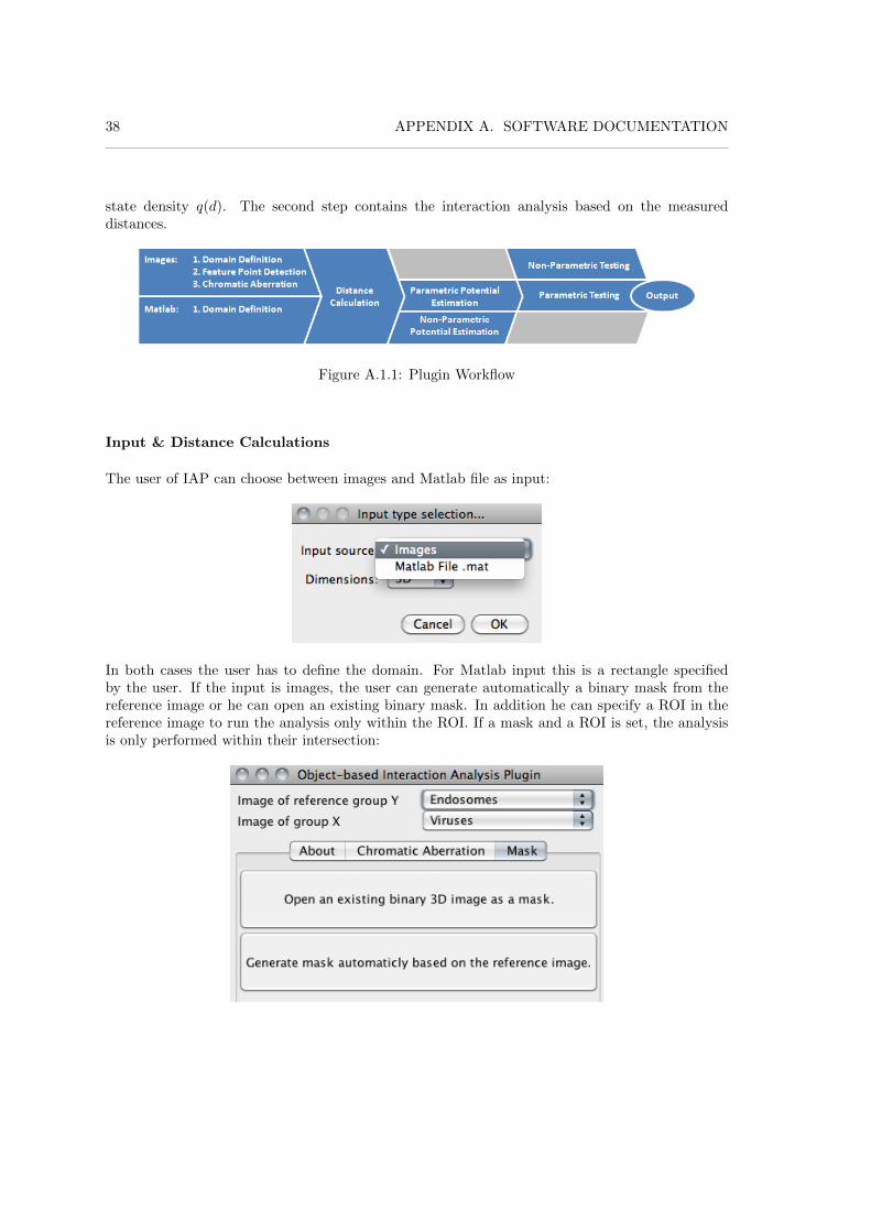
38 APPENDIX A. SOFTWARE DOCUMENTATION

state density q(d). The second step contains the interaction analysis based on the measureddistances.

Figure A.1.1: Plugin Workflow

Input & Distance Calculations

The user of IAP can choose between images and Matlab file as input:

In both cases the user has to define the domain. For Matlab input this is a rectangle specifiedby the user. If the input is images, the user can generate automatically a binary mask from thereference image or he can open an existing binary mask. In addition he can specify a ROI in thereference image to run the analysis only within the ROI. If a mask and a ROI is set, the analysisis only performed within their intersection:

38

Work Flow 39

Figure A.1.2: Automatically generated Mask based on reference image.

Relative shifts in the position of the objects due to chromatic aberration can be correct by a linearcalibration function. The IAP has the functionality to estimate the calibration function with theindependent plugin CA:

39


If object position detection is needed (in case of images as input), the detection is performedinteractively as the first step of the distance calculation:

The actual distance calculations run then fully automatically.

Figure A.1.3: Interactive Particle Detection

Interaction Analysis

In a second step, IAP offers the choice of three different interaction analyses of the measureddistances to the user. The user can choose between:

• Non-Parametric Testing (A.1.5),

• Parametric Potential Estimation and Parametric Testing (A.1.6),

• Non-Parametric Potential Estimation (A.1.7).

All three analyses do not require any user interaction after setting the necessary parameters. AfterIAP has completed the selected analysis, it presents the results in a user-friendly format.

40

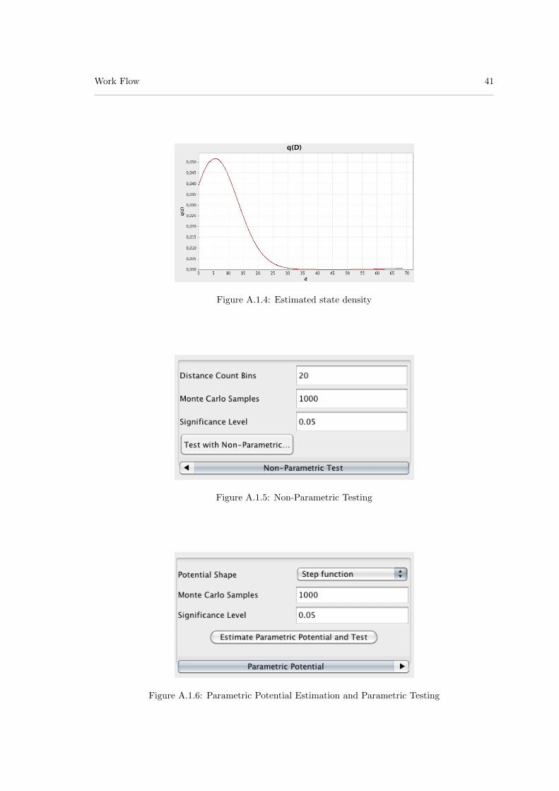
Work Flow 41

Figure A.1.4: Estimated state density

Figure A.1.5: Non-Parametric Testing

Figure A.1.6: Parametric Potential Estimation and Parametric Testing

41


Figure A.1.7: Non-Parametric Potential Estimation

Figure A.1.8: Estimated Parametric Potential

The examples for illustrating the features of IAP are based on a 3D dual color confocal image of aHER 911 cell. Rab5-positive endosomes and Adenovirus serotype 2 particles have been fluorescentlylabeled and an interaction analysis of these two groups of intra-cellular objects has produced theoutput shown in Figures A.1.2, A.1.3, A.1.4, and A.1.8.

A.2 Implementation

This section gives a short introduction into the code but will not discuss all details of the imple-mentation. For more details about the implementation of IAP, please refer to the documentedsource code.

A.2.1 Prerequisites to a Programmer

The plugin is implemented in the programming language Scala, so obviously Scala knowledge isan advantage. The transition from Java to Scala is relatively simple, so Java developers shouldhave no problem to read and understand the code, especially if they have basic knowledge offunctional programming. Basic concepts of Scala can be found on the official Scala web pagehttp://www.scala-lang.org or in the online available book “Programming Scala” from O’Reilly.Information about writing an ImageJ plugin can be found in the developer documentation ofImageJ http://rsbweb.nih.gov/ij/developer .

42

http://www.scala-lang.org



http://programming-scala.labs.oreilly.com

http://rsbweb.nih.gov/ij/developer

http://rsbweb.nih.gov/ij/developer

Library Dependencies 43

A.2.2 Library Dependencies

IAP uses the following open source libraries:

Name Description UsageWeka Data Mining Software in Java kd-Tree for Nearest Neighbor SearchJMatIO Matlab’s MAT-file I/O in JAVA Reading .mat Matlab Files.Scalala Scala Linear Algebra library Basic Linear Algebra CalculationsScalaNLP Scala library for Natural Language Processing, Monte Carlo Sampling

Machine Learning, and StatisticsCMA-ES CMA-ES Optimization in Java Potential Parameter Estimation

A.2.3 Packages

IAP has a modular architecture. Each module is in a seperate package:

mosaic.plugins ImageJ Pluginsmosaic.interaction Model Classesmosaic.interaction.input Image Handling and Input Generation for Modelmosaic.core.detection Feature Point Detection and Linkingmosaic.core.sampling Monte Carlo Sampling and Hypothesis Testsmosaic.core.distance Nearest Neighbor Distance Calculationsmosaic.core.optimization Potential Parameter Estimation

A.2.4 Important Classes

The main classes of IAP are listed below:

mosaic.interaction.InteractionModel Main Model Functionalitymosaic.interaction.InteractionGUI Graphical User Interface and Work Flowmosaic.plugin.ChromaticAberration Independent CA Plugin

43


44

BIBLIOGRAPHY 45

Bibliography

[1] M. D. Abramoff, P. J. Magelhaes, and S. J. Ram. Image processing with ImageJ. BiophotonicsInt., 11(7):36–42, 2004.

[2] R. Assuncao. Score test for pairwise interaction parameters of gibbs point processes. BrazilianJournal of Probability and Statistics, 17:169–178, 2003.

[3] M. Baron. Probability and Statistics for Computer Science. CRC Press, 2007.

[4] W. Baumeister. From proteomic inventory to architecture. FEBS Letters, 579(4):933–937,February 2005.

[5] S. Bolte and F. P. Cordelieres. A guided tour into subcellular colocalization analysis in lightmicroscopy. J. Microsc., 224:213–232, 2006.

[6] K. P. Burnhem and D. Anderson. Model Selection and Multi-Model Inference. Springer, 2ndedition, 2002.

[7] L. Stirling Churchman, Henrik Flyvbjerg, and James A. Spudich. A non-gaussian distributionquantifies distances measured with fluorescence localization techniques. Biophysical Journal,90(2):668 – 671, 2006.

[8] S.V. Costes, D. Daelemans, E.H. Cho, Z. Dobbin, G. Pavlakis, and S. Lockett. Automatic andquantitative measurement of protein-protein colocalization in live cells. Biophysical Journal,86(6):3993–4003, June 2004.

[9] L. Devroye. Non-uniform random variate generation. Springer-Verlag New York Inc., 1986.

[10] B. N. G. Giepmans, S. R. Adams, M. H. Ellisman, and R. Y. Tsien. Review - the fluorescenttoolbox for assessing protein location and function. Science, 312:217–224, 2006.

[11] N. Hansen. The cma evolution strategy: A comparing review. Towards a New EvolutionaryComputation, 192:75–102, 2006.

[12] J. Heikkinen and A. Penttinen. Bayesian smoothing in the estimation of the pair potentialfunction of gibbs point processes. Bernoulli, 5:1119–1136, 1999.

[13] S. W. Hell. Microscopy and its focal switch. Nature Methods, 6(1):24–32, December 2008.

[14] J. A. Helmuth, G. Paul, and I. F. Sbalzarini. Beyond co-localization: inferring spatial inter-actions between sub-cellular structures from microscopy images.; bmc bioinformatics. BMCbioinformatics, 11:372–372, 2010.

[15] E. A. Jares-Erijman and T. M. Jovin. Imaging molecular interactions in living cells by FRETmicroscopy. Curr. Opin. Chem. Biol., 10(5):409–416, 2006.

45

46 BIBLIOGRAPHY

[16] M. Kozubek and P. Matula. An efficient algorithm for measurement and correction of chro-matic aberrations in fluorescence microscopy. J. Microsc., 200:206–217, 2000.

[17] Q. Li. A syntaxin 1, g alpha o, and n-type calcium channel complex at a presynaptic nerveterminal: analysis by quantitative immunocolocalization; the journal of neuroscience. Thejournal of neuroscience, 24(16):4070, 2004.

[18] E. M. Manders, J. Stap, G. J. Brakenhoff, R. Van Driel, and J. A. Aten. Dynamics of three-dimensional replication patterns during the s-phase, analysed by double labelling of dna andconfocal microscopy.; journal of cell science. Journal of cell science, 103(3):857–862, 1992.

[19] J. Nocedal and Wright S. J. Numerical Optimization. Springer, 2nd edition, 2006.

[20] K. D. G. Pfleger and K. A. Eidne. Illuminating insights into protein-protein interactions usingbioluminescence resonance energy transfer (BRET). Nature Methods, 3(3):165–174, 2006.

[21] S. Rey, J. L. Gardy, and F. S. L. Brinkman. Assessing the precision of high-throughput com-putational and laboratory approaches for the genome-wide identification of protein subcellularlocalization in bacteria.; bmc genomics. BMC genomics, 6:162–162, 2005.

[22] I. F. Sbalzarini and P. Koumoutsakos. Feature point tracking and trajectory analysis for videoimaging in cell biology. Journal of Structural Biology, 151(2):182–95, Aug 2005.

[23] R. E. Thompson. Precise nanometer localization analysis for individual fluorescent probes;biophysical journal. Biophysical journal, 82(5):2775, 2002.

[24] B. Van Steensel. Partial colocalization of glucocorticoid and mineralocorticoid receptors indiscrete compartments in nuclei of rat hippocampus neurons; journal of cell science. J CELLSCI; Journal of cell science, 109:787, 1996.

[25] L. Wasserman. All of Nonparametric Statistics (Springer Texts in Statistics). Springer, 2007.

46

47

Acknowledgements

I want to thank Jo Helmuth for the idea of the thesis, the fertile collaboration and his importantsupport. It was motivating and interesting for me to work together with him as my advisor. Hewas always patient, open for questions, and very flexible. Furthermore, I would like to thank Prof.Ivo Sbalzarini for the opportunity to write this thesis in his group and for mentoring me duringmy master studies.

When I got stuck during the implementation phase, it was Thomas Pluss who gave me anotherperspective of the problem and helped me to debug the programm. I’m indebted for many invalu-able discussions with Gabriel Krummenacher during lunch time and for sharing the experience ofwriting a master thesis. Stefan Schori and Thomas Sommer were both benevolent and provident,I enjoyed to be their flat mate.

This master thesis marks the end of my studies at ETHZ and the end of my privileged education.I feel grateful to have been in the lucky situation to study abroad and at very good schools whichprepared me for my future life. Since I was born, it has always been my parents who supportedme, in a liberal manner. They financed me and I want to thank my parents for that. Specialthanks go to my family for everything these exceptional people have done for me. They taught methe courage to go self-reliant my way, the respect for my neighbors, and the discipline to work formy goals. Only this together with the necessary good luck made it possible to combine my studieswith my passion for sport.

47

Documents

Computational Analysis of Spatial Point Patterns for Cell ...mosaic.mpi-cbg.de/docs/Sutter2010.pdf · Computational Analysis of Spatial Point Patterns for Cell Organelles Master Thesis