Computational techniques for spatial logistic regression with large

datasets

Christopher J. Paciorek∗

April 19, 2007

key words: Bayesian statistics, disease mapping, Fourier basis, generalized linear mixed model, geo-

statistics, risk surface, spatial statistics, spectral basis

NOTICE: this is the author’s version of a work that was accepted for publication in Computational

Statistics and Data Analysis. Changes resulting from the publishing process, such as peer review, editing,

corrections, structural formatting, and other quality control mechanisms may not be reflected in this docu-

ment. Changes may have been made to this work since it was submitted for publication. A definitive version

was subsequently published in Computational Statistics and Data Analysis, 51, 3631-3653, (2007). DOI

10.1016/j.csda.2006.11.008

1 Abstract

In epidemiological research, outcomes are frequently non-normal, sample sizes may be large, and effect

sizes are often small. To relate health outcomes to geographic risk factors, fast and powerful methods for

fitting spatial models, particularly for non-normal data, are required. I focus on binary outcomes, with

the risk surface a smooth function of space, but the development herein is relevant for non-normal data in

general. I compare penalized likelihood models, including the penalized quasi-likelihood (PQL) approach,

and Bayesian models based on fit, speed, and ease of implementation.

A Bayesian model using a spectral basis representation of the spatial surface provides the best tradeoff of

sensitivity and specificity in simulations, detecting real spatial features while limiting overfitting and being

more efficient computationally than other Bayesian approaches. One of the contributions of this work is∗Christopher Paciorek is Assistant Professor, Department of Biostatistics, Harvard School of Public Health, 655 Huntington

Avenue, Boston, MA 02115 (E-mail: paciorek@alumni.cmu.edu).

1

further development of this underused representation. The spectral basis model outperforms the penalized

likelihood methods, which are prone to overfitting, but is slower to fit and not as easily implemented. A

Bayesian Markov random field model performs less well statistically than the spectral basis model, but is

very computationally efficient. We illustrate the methods on a real dataset of cancer cases in Taiwan.

The success of the spectral basis with binary data and similar results with count data suggest that it may

be generally useful in spatial models and more complicated hierarchical models.

2 Introduction

Epidemiological investigations that assess how health outcomes are related to risk factors that vary geo-

graphically are becoming increasingly popular. This paper is motivated by an ongoing epidemiological

study in Kaohsiung, Taiwan, a center of petrochemical production, for which administrative data suggest

excess cancer deaths amongst residents less than 20 years old living within 3 km of a plant (Pan et al. 1994).

A full case-control study is in progress to investigate this suspected link between plant emissions and can-

cer, with the residences of individuals being geocoded to allow for spatial modelling. Such individual-level

or point-referenced data are becoming increasingly common in epidemiology with the use of geographic

information systems (GIS) and geocoding of addresses. In contrast to health data aggregated into regions,

often fit using Markov random field (MRF) models (Waller et al. 1997; Best et al. 1999; Banerjee et al.

2004), analysis of individual-level data (often called geostatistics) avoids both ecological bias (Greenland

1992; Richardson 1992; Best et al. 2000) and reliance on arbitrary regional boundaries, but introduces com-

putational difficulties.

In this paper, I focus on methods for fitting models for Bernoulli response data with the outcome a binary

variable indicating disease or health status, but my development is relevant for non-normal data in general.

The specific model I investigate is a logistic regression,

Yi ∼ Ber(p(xi, si))

logit(p(xi, si)) = xiT β + g(si;θ), (1)

where Yi, i = 1, . . . n, is the binary status of the ith subject; g(·;θ) is a smooth function, parameterized by

θ, of the spatial location of subject i, si ∈ <2; and xi is a vector of additional individual-level covariates of

interest. One application of this model is to the analysis of case-control data. For binary outcomes with the

logit link, the use of a retrospective case-control design in place of random sampling from the population

increases the power for assessing relative risk based on the covariates, including any spatial effect, but

2

prevents one from estimating the absolute risk of being a case (Prentice and Pyke 1979; Elliott et al. 2000;

Diggle 2003, pp. 133-143).

There have been several approaches to modelling the smooth function, g(·;θ), each with a variety of

parameterizations. One basic distinction is between deterministic and stochastic representations. In the

former, (1) is considered a generalized additive model (GAM) (Hastie and Tibshirani 1990; Wood 2006),

e.g. using a thin plate spline or radial basis function representation for g(·;θ), with the function estimated via

a penalized approach. The stochastic representation considers the smooth function to be random, either as a

collection of correlated random effects (Ruppert et al. 2003), or as an equivalent stochastic process, such as

in kriging (Cressie 1993), which takes g(·;θ) to be a Gaussian process. Of course in the Bayesian paradigm,

the unknown function is always treated as random with a (perhaps implicit) prior distribution over functions.

Note that from this perspective, the GAM can be expressed in an equivalent Bayesian representation, and

there are connections between the thin plate spline and stochastic process approaches (Cressie 1993; Nychka

2000) and also between thin plate splines and mixed model representations (Ruppert et al. 2003).

While models of the form (1) have a simple structure, fitting them can be difficult for non-Gaussian re-

sponses. If the response were Gaussian, there are many methods, both classical and Bayesian, for estimating

β, g(·;θ), and θ. Most methods rely on integrating g(·;θ) out of the model to produce a marginal likelihood

or posterior. In the non-Gaussian case, this integration cannot be done analytically, which leads to substan-

tial difficulty in fitting the model because of the high dimensional quantities that need to be estimated. Initial

efforts to fit similar models have focused on approximating the integral in the GLMM framework or fitting

the model in a Bayesian fashion. In the case of binary data, the approximations used in the GLMM frame-

work may be poor (Breslow 2003) and standard Markov chain Monte Carlo (MCMC) techniques for the

Bayesian model exhibit slow mixing (Christensen et al. 2006). More recent efforts have attempted to over-

come these difficulties; this paper focuses on comparing promising methods and making recommendations

relevant to practitioners.

My goal in this paper is to investigate methods for fitting models of the form (1). I describe a set

of methods (Section 3) that hold promise for good performance with Bernoulli and other non-Gaussian

data and large samples (hundreds to thousands of individuals) and detail their implemention in Section 4.

One of these methods, the spectral basis approach of Wikle (2002), has seen limited use; I develop the

approach in this context by simplifying the model structure and devising an effective MCMC sampling

scheme. I compare the performance of the methods on simulated epidemiological data (Section 5) as well

as preliminary data from the Taiwan case-control study (Section 6). In evaluating the methods, my primary

criteria are the accuracy of the fit, speed of the fitting method, and ease of implementation, including the

3

availability of software. I close by discussing extensions of the models considered here and considering the

relative merits and shared limitations of the methods.

3 Overview of methods

The methods to be discussed fall into two categories: penalized likelihood models fit via iteratively weighted

least squares and Bayesian models fit via MCMC, but there are connections between all of them. First I

describe two penalized likelihood methods, one in which the objective function arises from an approximation

to the marginal likelihood in a mixed effects model, and a second in which the penalized likelihood is the

original objective function of interest. Next I present several Bayesian methods, three of which use basis

function representations of the spatial effect, while one takes an MRF approach. Two of the methods (one

penalized likelihood and one Bayesian) are motivated by the random effects framework, but can also be

viewed as basis function representations of a regression term. I close the section by briefly mentioning some

other methods of less promise for my purposes.

For both penalized likelihood and Bayesian models, in the Gaussian response setting, the unknown

spatial function can be integrated out of the model. This integration leaves a small number of parameters

to be estimated based on the marginal likelihood or marginal posterior, often using numerical maximization

or MCMC. In a generalized model such as (1), fitting the model is difficult because the spatial process, or

equivalently the basis coefficients or random effects, cannot be integrated out of the model in closed form;

estimating the high-dimensional quantities in the model poses problems for both penalized likelihood and

Bayesian approaches. At their core, both of the penalized likelihood methods described here use iterative

weighted fitting approaches to optimize the objective function. In the Bayesian methods (apart from the

MRF approach), the spatial function is represented by a basis function representation and fit via MCMC;

in some cases this representation is an approximation of a Gaussian process (GP). The methods employ a

variety of parameterizations and computational tricks to improve computational efficiency.

To simplify the notation I use gs to denote the vector of values calculated by evaluating g(·) for each

of the elements of s (i.e., for each observation location), namely gs = (g(s1), . . . , g(sn))T . I suppress the

dependence of g(·) and gs on θ.

4

3.1 Penalized likelihood-based methods

3.1.1 Penalized likelihood and GLMMs

When the spatial function is represented as a random effects term, gs = Zu, model (1) is an example of

a GLMM, with the variance of the random effects serving to penalize complex functions. Kammann and

Wand (2003) recommend specifying Z and Cov(u) = Σ such that Cov(Zu) = ZΣZT is a reasonable

approximation of the spatial covariance structure of gs for the problem at hand. Kammann and Wand (2003)

suggest constructing Z based on the Matérn covariance, which takes the form,

C(τ) =1

Γ(ν)2ν−1

(2√

ντ

ρ

)ν

Kν

(2√

ντ

ρ

), (2)

where τ is distance, ρ is the range (correlation decay) parameter, and Kν(·) is the modified Bessel function

of the second kind, whose order is the differentiability parameter, ν > 0. This covariance function has

the desirable property that sample functions of GPs parameterized with the covariance are bν − 1c times

differentiable. As ν → ∞, the Matérn approaches the squared exponential form, with infinitely many

sample path derivatives, while for ν = 0.5, the Matérn takes the exponential form with no sample path

derivatives. Ngo and Wand (2004) suggest basing Z on the generalized covariance function corresponding

to thin plate spline regression (see section 3.1.2 for details on this generalized covariance). Both approaches

take Σ = σ2uI . Z is constructed as Z = ΨΩ−

12 , where the elements of Ψ are the (generalized) covariances

between the data locations and the locations of a set of pre-specified knots, κk, k = 1, . . . ,K,

Ψ = (C(‖ si − κk ‖)) i=1,...,n;k=1,...,K .

The matrix Ω has a similar form, but with pairwise (generalized) covariances amongst the knot locations.

Kammann and Wand (2003) call this approach low-rank kriging because it is based on a parsimonious

set of K < n knots, which reduces the computational burden. This parameterization can be motivated

by noticing that if a knot is placed at each data point and the basis coefficients are taken to be normal,

then gs = Zu ∼ N (0, σ2uC) ⇒ g(·) ∼ GP(0, σ2

uC(·, ·)); i.e., g(·) has a GP prior distribution whose

(generalized) covariance function, C(·, ·), is the covariance used in calculating the elements of Ψ and Ω.

Fixing Z in advance forces σ2u to control the amount of smoothing, allowing the model to be fit using

standard mixed model software; for this reason Kammann and Wand (2003) fix ρ and ν in advance. Whether

this overly constrains model fitting remains an open question, on which I touch in the discussion. One can

also think of the GLMM representation as a radial (i.e., isotropic) basis representation for the spatial surface,

with coefficients, u, and basis matrix, Z.

5

Representing the spatial model as a GLMM seemingly makes available the variety of fitting methods

devised for GLMMs, but many of these are not feasible for the high-dimensional integrals involved in spatial

models. Most GLMM research that explicitly considers spatial covariates focuses on Markov random field

(MRF) approaches to modelling the spatial structure based on areal data (e.g., Breslow and Clayton 1993;

Fahrmeir and Lang 2001; Banerjee et al. 2004). Here I have individual-based data, so I use the penalized

quasi-likelihood (PQL) approach of Breslow and Clayton (1993) and Wolfinger and O’Connell (1993),

who arrived independently at an iterative weighted least squares (IWLS) procedure for fitting GLMMs,

maximizing the objective function,

− 12φ

n∑i=1

di(yi, g(xi, si))−12uTΣ−1u, (3)

where φ is a dispersion parameter and di(·) is the deviance, the log-likelihood up to a constant. REML is

used to re-estimate the variance component(s) at each iteration. The approximations involved in arriving at

the objective function (3) are generally thought to be poor for clustered binary data, resulting in biased esti-

mates (Breslow 2003), although there is evidence that the method works well in the spatial setting (Hobert

and Wand 2000; Wager et al. 2004), where the GLMM setup is merely a computational tool allowing estima-

tion using mixed effects model software. The crux of the matter lies not in the accuracy of the approximation

of the true integrated likelihood by (3), but in the appropriateness of (3) as a penalized log-likelihood ob-

jective function, in particular the form of the penalty term, the adequacy of REML in estimating the penalty

(variance component) with binary data, and the performance of IWLS with the nested REML estimation.

3.1.2 Penalized likelihood and generalized cross-validation

Wood (2000, 2003, 2004) also proposes iterative weighted fitting of reduced rank thin plate splines with

estimation of a smoothing parameter at each iteration, but he uses a different computational approach. Thin

plate splines are higher-dimensional extensions of smoothing splines and can be seen as a special case of

a Gaussian process model, with generalized covariance (Cressie 1993, p. 303; O’Connell and Wolfinger

1997) characterized in terms of distance, τ . The form in two dimensions is

C(τ) ∝ τ2m−2 log(τ),

where m is the order of the spline (commonly two, giving an L2 penalty).

For computational efficiency, Wood (2003) approximates the thin plate spline generalized covariance

basis matrix, Z, by a truncated eigendecomposition, Z, which gives the following form for the spatial

function,

g(si) = φiT α + zi

T u,

6

where φiT α are unpenalized polynomial terms. The method then optimizes a penalized log-likelihood with

penalty term, λuT Zu. The penalized log-likelihood objective function is similar to the GLMM objective

function (3), and is also maximized using penalized IWLS, but with the smoothing penalty, λ, optimized at

each iteration by an efficient generalized cross-validation (GCV) method (Wood 2000, 2004). The similar-

ities between this approach and the GLMM approach suggest that they may give similar answers, although

there are differences in the simulation results in Section 5.3.1. One difference is that the GLMM spatial

model uses a set of knots to reduce the rank of Z, whereas the eigendecomposition is used here (but note

that the number of knots can also be restricted in this approach). A second difference is the use of GCV

rather than REML to estimate the smoothing parameter at each iteration. As with the GLMM approach the

important estimation issues include the performance of the GCV criteria chosen to optimize the penalty term

and the numerical performance of the iterative algorithm with nested penalty optimization.

3.2 Bayesian methods

In most Bayesian models, the spatial function is represented as a Gaussian process or by a basis function

representation. Diggle et al. (1998) introduced generalized geostatistical models, with a latent Gaussian

spatial process, as the natural extension of kriging models to exponential family responses. They used

Bayesian estimation, suggesting a Metropolis-Hastings implementation, with the spatial function sampled

sequentially at each observation location at each MCMC iteration. However, as shown in their examples

and discussed elsewhere (Christensen et al. 2000; Christensen and Waagepetersen 2002; Christensen et al.

2006), this implementation is slow to converge and mix, as well as being computationally inefficient because

of the inverse covariance matrix involved in calculating the prior for gs.

An alternative approach, which avoids large matrix inversions, is to express the unknown function in

a basis, gs = Zu, where Z contains the basis function values evaluated at the locations of interest, and

estimate the basis coefficients, u (e.g., Higdon 1998). When the coefficients are normally distributed, this

representation can be viewed as a GP evaluated at a finite set of locations, with Cov(gs) = ZCov(u)ZT .

Two of the methods described below use such basis function approximations to a stationary GP, while the

third, a neural network model, relies on a basis function representation that, while not explicitly designed

to approximate a particular stationary GP, does give an implicit GP prior distribution for the spatial process,

and has been shown to have a close connection to GP models (Neal 1996).

The fourth method, which I have added at the suggestion of a reviewer, considers a Markov random field

representation of the unknown function on a grid.

7

3.2.1 Bayesian GLMMs

Zhao and Wand (2005) model the spatial function by approximating a stationary GP using the basis function

representation, gs = Zu, given in the penalized likelihood setting in Section 3.1.1. They specify a Bayesian

model, with u ∼ N (0, σ2uI), the prior distribution over the basis coefficients, and fit the model via MCMC.

As suggested in Kammann and Wand (2003), Zhao and Wand (2005) fix the covariance parameters, taking

ν = 1.5 and

ρ = maxi,j=1,...,n

‖ si − sj ‖,

and letting the variance parameter σ2u control the degree of smoothing. One could estimate ρ and ν in

the MCMC, as well as include anisotropy parameters in the covariance calculations, but this would require

recalculating Ψ and Ω−12 at each iteration, which would slow the fitting process and likely produce slower

mixing.

3.2.2 Bayesian spectral basis representation

A second method that improves computational efficiency by using basis functions to approximate a station-

ary GP is a spectral, or Fourier, representation. Isotropic GPs can be represented in the Fourier basis, which

allows one to use the Fast Fourier Transform (FFT) to speed calculations. Here I describe the basic approach

in two-dimensional space, following Wikle (2002); I leave the details of my implementation to Section 4.4,

with further description of the spectral basis construction in the appendix.

The key to the spectral approach is to approximate the function g(·) on a grid, s#, of size K = k1× k2,

where k1 and k2 are powers of two. Evaluated at the grid points, the vector of function values is represented

as

gs# = Zu, (4)

where Z is a matrix of orthogonal spectral basis functions, and u is a vector of complex-valued basis coef-

ficients, um = am + bmi, m = 1, . . . ,K. The spectral basis functions are complex exponential functions,

i.e., sinusoidal functions of particular frequencies; constraints on the coefficients ensure that gs# is real-

valued and can be expressed equivalently as a sum of sine and cosine functions. To approximate mean zero

stationary GPs, the basis coefficients have the prior distribution, a

b

∼ N (0,Σθ) (5)

where the diagonal (asymptotically, see Shumway and Stoffer (2000, Section T3.12)) covariance matrix

of the basis coefficients, Σθ, parameterized by θ, can be expressed in closed form (for certain covariance

8

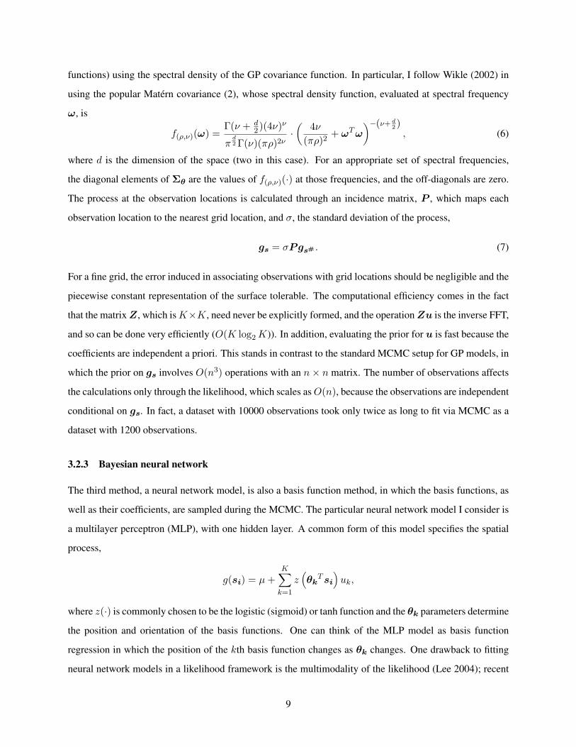
functions) using the spectral density of the GP covariance function. In particular, I follow Wikle (2002) in

using the popular Matérn covariance (2), whose spectral density function, evaluated at spectral frequency

ω, is

f(ρ,ν)(ω) =Γ(ν + d

2)(4ν)ν

πd2 Γ(ν)(πρ)2ν

·(

4ν

(πρ)2+ ωT ω

)−(ν+ d2 )

, (6)

where d is the dimension of the space (two in this case). For an appropriate set of spectral frequencies,

the diagonal elements of Σθ are the values of f(ρ,ν)(·) at those frequencies, and the off-diagonals are zero.

The process at the observation locations is calculated through an incidence matrix, P , which maps each

observation location to the nearest grid location, and σ, the standard deviation of the process,

gs = σPgs# . (7)

For a fine grid, the error induced in associating observations with grid locations should be negligible and the

piecewise constant representation of the surface tolerable. The computational efficiency comes in the fact

that the matrix Z, which is K×K, need never be explicitly formed, and the operation Zu is the inverse FFT,

and so can be done very efficiently (O(K log2 K)). In addition, evaluating the prior for u is fast because the

coefficients are independent a priori. This stands in contrast to the standard MCMC setup for GP models, in

which the prior on gs involves O(n3) operations with an n× n matrix. The number of observations affects

the calculations only through the likelihood, which scales as O(n), because the observations are independent

conditional on gs. In fact, a dataset with 10000 observations took only twice as long to fit via MCMC as a

dataset with 1200 observations.

3.2.3 Bayesian neural network

The third method, a neural network model, is also a basis function method, in which the basis functions, as

well as their coefficients, are sampled during the MCMC. The particular neural network model I consider is

a multilayer perceptron (MLP), with one hidden layer. A common form of this model specifies the spatial

process,

g(si) = µ +K∑

k=1

z(θk

T si

)uk,

where z(·) is commonly chosen to be the logistic (sigmoid) or tanh function and the θk parameters determine

the position and orientation of the basis functions. One can think of the MLP model as basis function

regression in which the position of the kth basis function changes as θk changes. One drawback to fitting

neural network models in a likelihood framework is the multimodality of the likelihood (Lee 2004); recent

9

work has focused on specifying Bayesian neural network models and fitting the models via MCMC (Neal

1996; Lee 2004).

3.2.4 Bayesian Markov random fields

In the context of areal data, MRF models (Rue and Held 2005) are very popular and are computationally

simple to fit using MCMC because areal units can be updated individually. Following the discussion in

Section 3.2.2 that with a fine enough grid, a gridded representation of the surface is likely to be sufficient,

I consider a MRF model for the spatial process evaluated on a grid, gs# . Here instead of a Gaussian

process representation, I make use of a Gaussian MRF (GMRF) in which the conditional distribution of the

process at any location, gi, depends only on a small number of neighbors: a common specification gives

gi|gj , j 6= i ∼ N (∑

j∼i gj/ni, (τ2ni)−1) where j ∼ i indicates that the jth location is a neighbor of the

ith location, and ni is the number of neighbors. The neighborhood structure and the conditional precision

parameter, τ2, determine the strength of spatial association of the process. In the binary data context, use

of the Albert and Chib (1993) data augmentation approach with a probit link allows for Gibbs sampling to

be employed. Given the augmented data, the process values have a GMRF conditional distribution. In the

more general context of non-normal data, Rue et al. (2004) use Gaussian approximations to the conditional

distribution of gs|τ2,y in the context of Metropolis-Hastings sampling. The GMRF model allows the use

of computationally efficient algorithms based on sparse matrix calculations (the precision matrix of the

process, gs# , is sparse) to fit the model, which in addition to the gridding, can greatly speed fitting. Other

promising approaches built upon the GMRF structure, involving GMRF approximations to GPs (Rue and

Tjelmeland 2002; Rue and Held 2005) and fitting GMRF models without MCMC (Rue and Martino 2006)

are highlighted in the discussion.

3.3 Other methods

There are many methods designed for spatial data, usually for Gaussian responses, and for nonparametric

regression in general. In principle, most or all could be adapted for binary spatial data, but they would raise

many of the fitting issues already discussed in this paper. I mention a few of the methods here, but do not

include them in the empirical comparison because they lack readily available code or would need extensive

further development for application to binary spatial data.

In contrast to the approximation to the integral involved in the PQL approach, several papers have pro-

vided EM (McCulloch 1994, 1997; Booth and Hobert 1999), numerical integration (Hedeker and Gibbons

1994; Gibbons and Hedeker 1997), and MCMC (Christensen 2004) methods for maximizing the GLMM

10

likelihood. However, software for the approaches does not seem to be available, and the algorithms are

complex and computationally intensive; I do not consider these to be currently viable methods for practi-

tioners. Wahba et al. (1995) represent nonparametric functions as ANOVA-like sums of smoothing splines

and optimize a penalized log-likelihood in an iterative fashion, similar to the penalized methods described

previously. However, as noted by Wood (2004), the approach generally requires a parameter per data point,

making computations inefficient, and the only available software is a set of Fortran routines, which are less

user-friendly than desired here. The Bernoulli likelihood (1) can be expressed using data augmentation in a

way that allows for Gibbs sampling (Albert and Chib 1993) as the MCMC technique, but the computations

involve n× n matrices at each iteration; however note that I use a variant of this approach in the context of

an MRF model (Section 4.6). Holmes and Mallick (2003) extend the free-knot spline approach of Denison

et al. (2002) to generalized regression models. They fit the model via reversible-jump MCMC and have soft-

ware for the Gaussian model, but software for the generalized model was not available. For nonstationary

Gaussian data, authors have used mixture models, including mixture of splines (Wood et al. 2002) and mix-

ture of Gaussian processes (Rasmussen and Ghahramani 2002), in which the mixture weights depend on the

covariates (the spatial locations in my context), but this adds even more complexity to MCMC implemen-

tations and has not been developed for the generalized model. Finally, Christensen et al. (2006) develop a

data-dependent reparameterization scheme for improved MCMC performance and apply the approach with

Langevin updates that use gradient information; while promising, the approach is computationally intensive,

again involving n× n matrix computations at each iteration, and software is not available.

4 Implementation

Here I describe the implementation of each method, coded in R with the exception of the neural network and

MRF models, with descriptions of the prior distributions and MCMC sampling schemes for the Bayesian

models. The subsection headings indicate the abbreviations I use to denote the methods in discussing the

results.

4.1 Penalized likelihood and GLMMs (PL-PQL)

I follow the basic approach of Ruppert et al. (2003) and Ngo and Wand (2004), using the thin plate spline

basis and estimating the penalized likelihood model via the PQL approach. This can be performed with

standard software by iteratively calling a mixed model fitting routine designed for Gaussian responses. The

SemiPar library in R fits the model as does the gamm() function in the mgcv library; I used the spm()

11

function in the SemiPar library. I use an equally-spaced 8 × 8 grid of knot locations; using a 16 × 16 grid

had little effect on my empirical results in a sensitivity assessment. Additional covariates can be included

in a linear or smooth manner as described in Ngo and Wand (2004). Prediction at unobserved locations is

done efficiently using the estimated basis coefficients, u, and a prediction basis matrix, Zpred, constructed

in the same way as Z but with Ψpred containing the pairwise covariances between the knot locations and the

prediction locations. The SemiPar library provides uncertainty estimates.

I also ran the model with the Matérn covariance with fixed range and smoothness parameters, as sug-

gested by Kammann and Wand (2003), and found that the results varied depending on the value of the

range parameter. For the isotropic dataset, using the value of ρ = max ‖ si − sj ‖, the method performed

markedly worse than with the thin plate spline covariance, while choosing a value of ρ equal to one-fourth

the recommended value produced results similar to the thin plate spline-based model. This suggests that the

method is sensitive to the range parameter, but note Zhang (2004), who shows that σ2 and ρ cannot both be

estimated consistently.

4.2 Penalized likelihood and GCV (PL-GCV)

I use the gam() function from the mgcv library in R to fit the penalized likelihood model based on GCV,

using the default of a K = 30 dimensional basis, which appeared to be sufficient for my simulations

and data. The approach can handle additional covariates in a linear or smooth manner. The mgcv library

provides predictions at unobserved locations and uncertainty estimates for parameters and the spatial field;

there is a brief discussion of these uncertainty estimates for the generalized model in Wood (2003). One

drawback, shared by most of the other methods, is that the method, as implemented in R, is not designed for

anisotropy. In principle this could be handled using additional smoothing parameters (Wood 2000); Wood

(2003) mentions that work is in progress.

4.3 Bayesian GLMM (Geo)

For the Bayesian version of the GLMM approach, I follow Zhao and Wand (2005) but modify the approach

to improve MCMC performance. Zhao and Wand (2005) use vague proper Gaussian priors for the fixed

effect coefficients, β, (σ2β = 1010) and a vague inverse-gamma prior for the variance component, σ2

u ∼

IG(a = 0.5, b = 0.0005), with mean b/(a−1) (for a > 1). They fit the model via MCMC using Metropolis-

Hastings with t-distributed joint proposals of the weighted least squares type for the coefficients (β,u) , as

suggested by Gamerman (1997), and conjugate Gibbs sample updates for σ2u.

I tried this MCMC scheme, but made several changes to improve mixing; even with these changes, the

12

scheme did not mix as well as the spectral basis approach (Section 5.3.2). First, I found that t-distribution

proposals for the coefficients were rarely accepted because of the high variability in the proposals; I used a

multivariate normal proposal density with the same form for the mean and covariance (scale) matrix as Zhao

and Wand (2005), but with the covariance matrix multiplied by an tuneable constant, w, to achieve accep-

tance rates of approximately 0.22 for the coefficients. Rather than sampling β and u together, I separately

sampled β using a simple Metropolis proposal. Second, I found that the critical smoothing parameter, σ2u,

mixed very slowly when sampled via conjugate Gibbs updates, because of the strong dependence between

σ2u and u, a phenomenon observed in MRF models as well (Rue and Held 2005, pp. 142-143). Instead, fol-

lowing Paciorek (2003), I sampled σu jointly with the coefficients, u, as a block. As the first part of the joint

sample, I sampled σu using a Metropolis scheme. Then, conditional on the proposed value of σu, I sam-

pled u using the multivariate normal proposal density used for sampling u, described above, with w = 1,

accepting or declining σu,u together in one decision. My prior for σu was N (0, 1000), left-truncated at

0.001, with a normal proposal distribution centered on the current value. Sampling σu directly, rather than

on the log scale, allowed me to use the same proposal variance for all values of the parameter. I suspect that

slice sampling would work well for this parameter, but that it should still be employed in a joint sample of

σu and u.

I used an equally-spaced 8 × 8 grid of knot locations; using a 16 × 16 grid had little effect on my

empirical results in a sensitivity assessment. Prediction is done efficiently at each iteration in the same way

as described in Section 4.1. As described in Zhao and Wand (2005), additional smooth covariate terms can

be included in the model and fit in similar fashion to the spatial term.

Note that I did not apply this method to the 10000 observation cohort simulation because the multivariate

proposal density of Zhao and Wand (2005) involves matrix multiplications with K by n and n by n matrices.

An alternative approach in which the K basis coefficients were proposed based on a proposal distribution

with a diagonal covariance matrix would be substantially more efficient, but would likely show slower

mixing than the proposal used here.

4.4 Bayesian spectral basis (SB)

This approach is based on Wikle (2002) with modifications for this context and a custom sampling scheme.

Wikle (2002) embeds the spectral basis representation (4,7) in a hierarchical model that involves several

error components, including one relating gs to the likelihood and one relating Zu to gs# . my model omits

these additional error components, both for simplicity and because the modification allows for reasonably

fast MCMC mixing; the fact that the basis coefficients are directly involved in the likelihood (1), rather than

13

further from the data in the hierarchy of the model may help with mixing. In addition to the likelihood

(1) and the prior on u (5), I need only specify priors on β, σ, ρ, and ν. These are taken to be proper

but non-informative. In particular, for binary data with no additional covariates, I take β0 ∼ N (0, 10),

log σ ∼ N (0, 9), and ν ∼ U(0.5, 30). For ρ, I use a prior that favors smoother surfaces, taking ζ = log ρ

and f(ζ) ∝ ζ2I(ζ ∈ (−4.6, 1.35)). The exact form of this prior is not critical, except that forcing the range

parameter to remain in the interval is important to prevent it from wandering in extreme parts of the space

in which changes in the parameter have little effect on the likelihood.

For β and log σ I use Metropolis and Metropolis-Hastings proposals, respectively. I propose each of

log ρ and ν jointly with u. First I propose log ρ or ν using Metropolis-Hastings or Metropolis proposals,

respectively. Then, conditional on the proposed hyperparameter, I propose

u∗i = ui ·

√(Σθ∗)i,i√(Σθ)i,i

, i = 1, . . . ,K,

where θ∗ = (ρ∗, ν) or θ∗ = (ρ, ν∗) depending on which hyperparameter is being proposed. Modifying ui

based on its prior variance, (Σθ)i,i, allows the covariance hyperparameters to mix more quickly by avoiding

proposals for which the coefficients are no longer probable based on their new prior variances. Such a deter-

ministic proposal for u is a valid MCMC proposal so long as the Jacobian of the transformation is included

in the acceptance ratio, based on a modification of the argument in Green (1995). This joint sample is mo-

tivated by the strong nonlinear dependence between the hyperparameters and process values, considered in

the MRF context by Knorr-Held and Rue (2002). Both log σ and log ρ require Metropolis-Hastings sam-

pling with the proposal variances depending on the parameter value to achieve constant acceptance rates;

slice sampling may be a superior alternative for these parameters, allowing the proposal variance to adjust to

the parameter value. As described in the appendix, the spectral basis coefficients, u, are sampled in blocks

(grouped according to their corresponding frequencies) via Metropolis proposals.

I use a grid, s#, of size 64 × 64, but as noted in the appendix, this corresponds to an effective grid of

32 × 32. Code for implementing the model in R is given in the electronic supplement. Additional linear

covariates can be easily included, while smooth covariate terms can be included in the model using the

spectral basis representation (see also Lenk (1999)). Prediction, done at the grid locations, is implicit in the

estimation of gs# .

4.5 Bayesian neural network (NN)

I use the Flexible Bayesian Modeling software of R. Neal (http://www.cs.toronto.edu/~radford/

fbm.software.html); this software uses tanh functions for z(·) and vague, proper priors for the vari-

14

ous hyperparameters, with MCMC sampling done via a combination of Gibbs sampling and hybrid Monte

Carlo. I use the default prior specification given in the binary regression example in the software’s docu-

mentation. I fix the number of hidden units at a relatively large value, K = 50, to allow for a sufficiently

flexible function but minimize compational difficulties.

4.6 Bayesian Markov random field (MRF)

I consider the unknown process, gs# , on a 32×32 grid, to correspond to the spectral basis grid. To simplify

the sampling based on a Gaussian conditiona distribution for the process values, I introduce a vector of

augmented data values, w, with one value for each observation. Let P be a mapping matrix that maps grid

cells to data locations. Then the model is

w|gs# ∼ N (µ1 + Pgs# , I)n∏

i=1

1(

wi

(yi −

12

)> 0

)gs# ∼ N (0,Q),

where Q is the precision matrix induced by the neighborhood structure and where the indicator functions en-

sure that the augmented variables are positive when the observation is one and negative otherwise, following

Albert and Chib (1993). This approach replaces the logit transformation in (1) with the probit transforma-

tion. Note that the use of the probit is not strictly appropriate for estimating relative risks based on covariates

in the case-control context (Diggle 2003, p. 133), but the similarity of the probit and logit transformations

and the empirical results given in Section 5 suggest that this substitution is not cause for concern.

To construct Q, I use a neighborhood structure in which the eight surrounding grid cells are considered

to be neighbors. I use an intrinsic conditional autoregressive model (ICAR) prior distribution for the spatial

process, as discussed in Banerjee et al. (2004) and Rue and Held (2005). This prior is improper, but the pos-

terior is proper. Following Rue and Held (2005), I impose a sum to zero constraint as the prior is identified

only up to an additive constant. Results under the MRF approach were somewhat sensitive to the choice of

prior: I considered gamma priors of the form τ2 ∼ G(1, b), with mean, 1/b, for b ∈ 0.0001, 0.001, 0.01,

which are similar to priors used in Rue and Held (2005). For b = 0.0001 and b = 0.001, the estimated

spatial surfaces were too smooth; b = 0.01 seemed to provide a good compromise between sensitivity and

specificity. Note that this prior strongly penalizes very large values of τ2, but avoids the sharp peak near

zero of priors of the form G(ε, ε) with ε ≈ 0 (Gelman 2006).

I use the GMRFLib_blockupdate function in the GMRFLib library of H. Rue to sample the conditional

precision parameter, τ2, and the process values, gs# , as a block, conditional on the augmented data, w,

15

following the approach of Knorr-Held and Rue (2002). The elements of w are sampled from their individual

truncated normal conditional distributions.

5 Simulations

I evaluate the methods on five simulated datasets, allowing me to assess the methods in a variety of situa-

tions that are likely to arise in practice. The simulations allow me to explore estimation under basic spatial

structures plausible for large epidemiological datasets, in particular contrasting a constant spatial surface

with surfaces with single peaks and a surface with several peaks and troughs. Without further simulations, I

do not know if the results would generalize to more complicated surfaces, but since epidemiological investi-

gations often have insufficient power to detect any spatial heterogeneity, my simulations are a good starting

point. To focus on the spatial structure, I include only a mean and no covariates as the Xβ portion of the

model.

I assess the performance of the methods in estimating the known spatial surfaces, their computational

speed, and MCMC convergence for the Bayesian methods.

5.1 Datasets

The first four datasets mimic case-control data similar to those of the Taiwan example. The first dataset has

no spatial effect. The second has a point source-induced isotropic spatial effect with a single maximum in

the risk (probability) surface. The third has a point source-induced spatial effect with anisotropy to simulate

the effect of prevailing winds. The spatial domain of all three datasets is a square area 15 units on a side,

and the baseline risk of disease is 0.0003. For the latter two datasets, the exposure peak occurs at the middle

of the square and the risk there is four times the baseline risk. For the isotropic surface, the risk drops

off following a bivariate normal distribution with standard deviations of 1.5 and correlation of zero, while

for the anisotropic surface, the risk drops off following a bivariate normal with standard deviations of 3.75

and covariance of 0.8 · 3.75. The fourth dataset uses the same spatial domain, but has a more complicated

spatial risk surface (taken from Hwang et al. (1994, function 5)), with several peaks and troughs; I multiply

by 0.000183 to give a maximum risk about four times the baseline, as above, and a minimum risk about

4.5 × 10−6 of the baseline; i.e., in the troughs, there is essentially no risk. Sampling for all four of these

datasets mimics a case-control study. First, a population of individuals is located randomly in the area.

Based on the underlying risk surface, each individual is randomly assigned to have a health outcome or

not. n1 = 200 cases and n0 = 1000 controls are then randomly selected from the populations of affected

16

and unaffected individuals. The fifth dataset mimics a cohort study in which a group of individuals are

followed over time to determine which individuals develop disease. I select 10000 individuals randomly

from a metropolitan area of size 50 km by 50 km. There are four concentric squares (50 km by 50 km,

19 by 19, 9 by 9, and 3 by 3) with population density increasing toward the middle of the area from 500

individuals per square km in the outermost region to 3000, 7000, and finally 10000 in the inner square and

corresponding increasing risk of 0.10, 0.11, 0.12, and 0.13.

For each dataset, with fixed underlying spatial risk function, I evaluate each method on 50 data samples

in which the locations and health outcomes of individuals are sampled.

5.2 Assessment

In the case-control setting, the methods calculate p(si). This estimates the risk surface at a location condi-

tional on inclusion (indicated by ∆i = 1) in the study, pCOND(si) = P (Yi = 1|si,∆i = 1), rather than the

true marginal risk surface, pMARG(si) = P (Yi = 1|si), given in Section 5.1. The conditional and marginal

risk surfaces are offset by a constant on the logit scale (Carroll et al. 1995, p.184; Elliott et al. 2000). To

assess the accuracy of the conditional surfaces estimated by the methods, I compute the true value of the

conditional risk surface, pCOND(si) = pMARG(si) + log r, where r = (n1(1− P (Yi = 1))/(n0P (Yi = 1))

is the relative sampling intensity of cases and controls. Henceforth I refer only to the conditional risk sur-

faces, denoted p, dropping the subscript, COND, and considering the surface at a grid of test locations,

pm = p(s∗m), m = 1, . . . ,M .

I use several criteria to compare the fits from the various methods. The first is the mean squared error,

MSEsim = M−1∑Mm=1(pm − pm)2, where for the Bayesian models, p is the posterior mean. MSE is

not really appropriate for probabilities; a measure based on predictive density is more principled, so the

second measure uses the Kullback-Leibler (KL) divergence between the predictive density of test data given

the fitted surface, h(y∗m|pm), and the true density, h(y∗m|pm), where the integral over the true Bernoulli

distribution of observations at location m, H(y∗m|pm), is averaged over the grid of test locations,

KLsim,point =1M

M∑m=1

∫log

h(y∗m|pm)h(y∗m|pm)

dH(y∗m|pm)

=1M

M∑m=1

(pm log

pm

pm+ (1− pm) log

1− pm

1− pm

).

With the Bayesian approaches, I can also use the full posterior, averaging over the MCMC samples,

t = 1, . . . , T, to assess fit for a vector of test data, y∗ = (y∗1, . . . , y∗M ), again using the KL divergence, and

17

scaling by M,

KLsim,Bayes =1M

∫log

h(y∗|p)h(y∗|y)

dH(y∗|p) (8)

≈ 1M

logh(y∗|p)h(y∗|y)

(9)

=1M

logh(y∗|p)∫

h(y∗|p)Π(p|y)dp(10)

≈ 1M

M∑m=1

(y∗m log pm + (1− y∗m) log(1− pm)) (11)

− 1M

log1T

T∑t=1

M∏m=1

py∗mm,(t)(1− pm,(t))

1−y∗m . (12)

Note that the resulting quantity (11-12) calculates the predictive density of the test data (12) (the conditional

predictive ordinate approach of Carlin and Louis (2000, p. 220)) under each method relative to the predictive

density of the test data under the true distribution (11). Ideally, this calculation should average over many

samples of test data, y∗ (8), but I use only one for computational convenience (9). However, note that the

assessment over a large test set taken at many locations, M , allows the variability over locations to stand in

for the variability over test samples and that I compute KLsim,Bayes for each of 50 data samples from each

dataset.

To assess the uncertainty estimates of the methods, I compare the length and coverage of 95% confi-

dence and credible intervals over the true function values at the test locations. For PL-GCV, I calculate the

confidence intervals using 1.96 multiplied by the standard error from the predict.gam() function in the mgcv

library; similarly for PL-PQL using predict.spm() and transforming to the response scale. For the Bayesian

methods, I use the 2.5 and 97.5 percentiles of the iterates from the Markov chains. Uncertainty estimates

were not readily available for NN, so I omitted them from this analysis.

For the Bayesian methods, since mixing and convergence have been problems, I also assess MCMC

mixing speed. The different methods have different parameterizations, so this is largely qualitative, but I

directly compare the samples of the log posterior density, f(θ|y) (Cowles and Carlin 1996) (calculated up

to the normalizing constant), examining the autocorrelation and effective sample size (Neal 1993, p. 105),

ESS =T

1 + 2∑∞

d=1 ρd(f(θ|y)), (13)

where ρd(f(θ|y)) is the autocorrelation at lag d for the log posterior, truncating the summation at the lesser

of d = 10000 or the first d such that ρd(π(θ|y)) < 0.05. Since the real limitation is computational, I also

estimate ESS per processor hour, to scale the methods relative to the speed of computing each iteration.

18

5.3 Results

5.3.1 Quality of fit

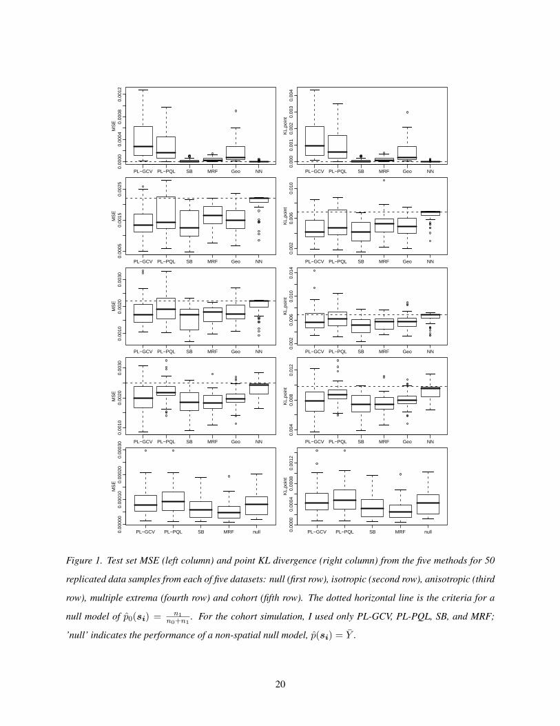
The spectral basis model provides the best compromise between sensitivity and specificity based on the

simulations, as shown in Figure 1. For the null dataset with no spatial effect, we see that the SB, MRF, and

NN models are markedly better than the other models in terms of MSE and point estimate KL divergence

(Fig. 1, row 1), with similar patterns when comparing amongst Bayesian models based on the full KL

divergence (not shown). NN outperforms SB, which in turn outperforms MRF, but all three have MSE

and KL divergence close to zero. By comparison the remaining models have MSE and KL far from zero,

clearly overfitting by finding features in the spatial surface that do not exist (not shown). All differences

are significant based on paired t-tests. I do not control for multiple testing as I merely wish to give a rough

idea of the signal to noise ratio; in most cases here and below in which there are significant differences, the

p-values are very small (p < 0.001).

The results for the isotropic, anisotropic, and multiple extrema case-control simulations (Figure 1, rows

2-4) show that NN avoids overfitting on the null dataset because it has little power to detect effects when

they do exist. It has much higher MSE and KL divergence than the other methods, approaching the MSE

and KL divergence of the null model, p0(si) = n1n0+n1

= 16 . In contrast, SB performs as well as the best

of the other methods (PL-GCV) on the isotropic dataset and outperforms all methods on the anisotropic

dataset. On the isotropic dataset, SB is significantly better than PL-GCV for KL divergence (p = 0.01)

but not for MSE (p = 0.29), while SB and PL-GCV are significantly better than the other methods except

that PL-GCV and Geo are not significantly different for KL (p = 0.18). On the anisotropic dataset, SB

is significantly better than the other methods, with no clear pattern of another method outperforming the

remaining methods. Except as noted, p < 0.001 for the SB method compared to the other methods. For

the multiple extrema dataset, SB, MRF and PL-GCV outperform the other methods, with slight evidence in

favor of SB and MRF over PL-GCV, and little to distinguish SB and MRF, except that SB is significantly

better than MRF for full KL divergence, suggesting that the posterior distribution from the SB model better

represents test data.

For the simulated cohort study, I compare only the PL-GCV, PL-PQL, SB, and MRF methods because

with n = 10000, the computations are too slow for the geoadditive model and the neural network. For this

dataset, SB and MRF outperform the penalized likelihood methods (p < 0.0001), which are not significantly

different (Figure 1, row 5). In contrast to the results for the case-control datasets, MRF is significantly better

than SB on all the criteria. SB and MRF are also significantly better than a constant null model, p(si) = Y ,

19

PL−GCV PL−PQL SB MRF Geo NN

0.00

000.

0004

0.00

080.

0012

MS

E

PL−GCV PL−PQL SB MRF Geo NN

0.00

00.

001

0.00

20.

003

0.00

4K

L,po

int

PL−GCV PL−PQL SB MRF Geo NN

0.00

050.

0015

0.00

25M

SE

PL−GCV PL−PQL SB MRF Geo NN

0.00

20.

006

0.01

0K

L,po

int

PL−GCV PL−PQL SB MRF Geo NN

0.00

100.

0020

0.00

30M

SE

PL−GCV PL−PQL SB MRF Geo NN

0.00

20.

006

0.01

00.

014

KL,

poin

t

PL−GCV PL−PQL SB MRF Geo NN

0.00

100.

0020

0.00

30M

SE

PL−GCV PL−PQL SB MRF Geo NN

0.00

40.

008

0.01

2K

L,po

int

PL−GCV PL−PQL SB MRF null0.00

000

0.00

010

0.00

020

0.00

030

MS

E

PL−GCV PL−PQL SB MRF null0.00

000.

0004

0.00

080.

0012

KL,

poin

t

Figure 1. Test set MSE (left column) and point KL divergence (right column) from the five methods for 50

replicated data samples from each of five datasets: null (first row), isotropic (second row), anisotropic (third

row), multiple extrema (fourth row) and cohort (fifth row). The dotted horizontal line is the criteria for a

null model of p0(si) = n1n0+n1

. For the cohort simulation, I used only PL-GCV, PL-PQL, SB, and MRF;

’null’ indicates the performance of a non-spatial null model, p(si) = Y .

20

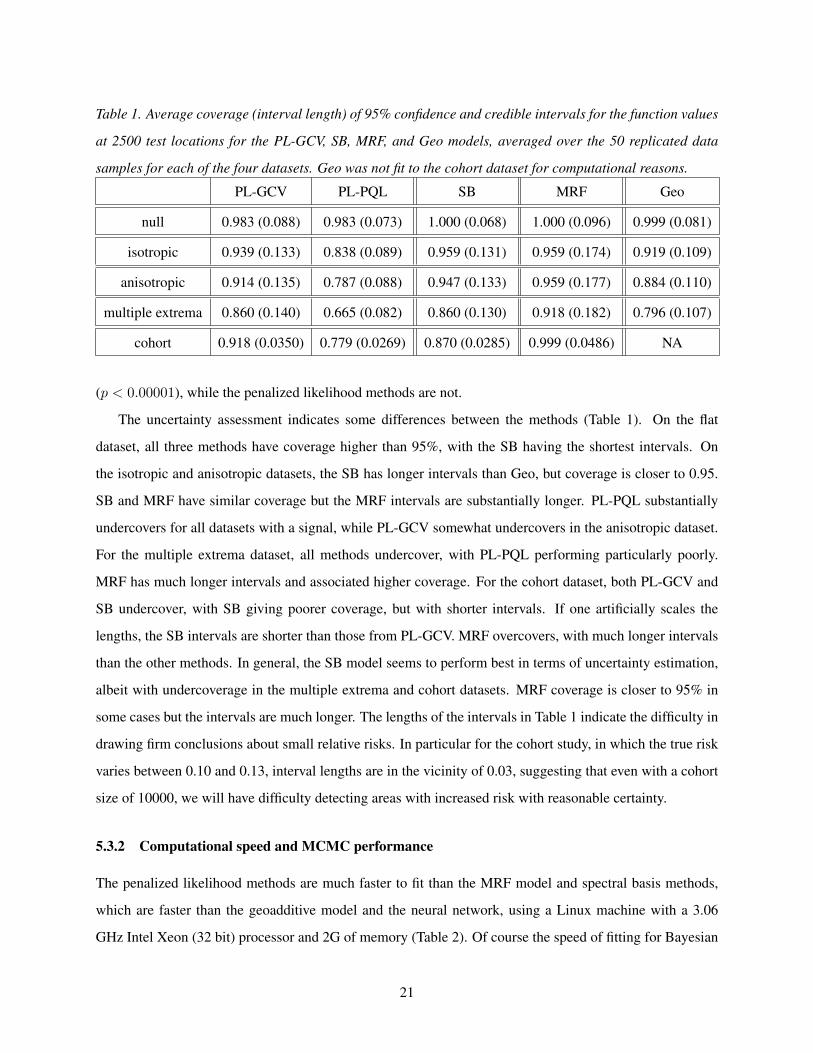
Table 1. Average coverage (interval length) of 95% confidence and credible intervals for the function values

at 2500 test locations for the PL-GCV, SB, MRF, and Geo models, averaged over the 50 replicated data

samples for each of the four datasets. Geo was not fit to the cohort dataset for computational reasons.

PL-GCV PL-PQL SB MRF Geo

null 0.983 (0.088) 0.983 (0.073) 1.000 (0.068) 1.000 (0.096) 0.999 (0.081)

isotropic 0.939 (0.133) 0.838 (0.089) 0.959 (0.131) 0.959 (0.174) 0.919 (0.109)

anisotropic 0.914 (0.135) 0.787 (0.088) 0.947 (0.133) 0.959 (0.177) 0.884 (0.110)

multiple extrema 0.860 (0.140) 0.665 (0.082) 0.860 (0.130) 0.918 (0.182) 0.796 (0.107)

cohort 0.918 (0.0350) 0.779 (0.0269) 0.870 (0.0285) 0.999 (0.0486) NA

(p < 0.00001), while the penalized likelihood methods are not.

The uncertainty assessment indicates some differences between the methods (Table 1). On the flat

dataset, all three methods have coverage higher than 95%, with the SB having the shortest intervals. On

the isotropic and anisotropic datasets, the SB has longer intervals than Geo, but coverage is closer to 0.95.

SB and MRF have similar coverage but the MRF intervals are substantially longer. PL-PQL substantially

undercovers for all datasets with a signal, while PL-GCV somewhat undercovers in the anisotropic dataset.

For the multiple extrema dataset, all methods undercover, with PL-PQL performing particularly poorly.

MRF has much longer intervals and associated higher coverage. For the cohort dataset, both PL-GCV and

SB undercover, with SB giving poorer coverage, but with shorter intervals. If one artificially scales the

lengths, the SB intervals are shorter than those from PL-GCV. MRF overcovers, with much longer intervals

than the other methods. In general, the SB model seems to perform best in terms of uncertainty estimation,

albeit with undercoverage in the multiple extrema and cohort datasets. MRF coverage is closer to 95% in

some cases but the intervals are much longer. The lengths of the intervals in Table 1 indicate the difficulty in

drawing firm conclusions about small relative risks. In particular for the cohort study, in which the true risk

varies between 0.10 and 0.13, interval lengths are in the vicinity of 0.03, suggesting that even with a cohort

size of 10000, we will have difficulty detecting areas with increased risk with reasonable certainty.

5.3.2 Computational speed and MCMC performance

The penalized likelihood methods are much faster to fit than the MRF model and spectral basis methods,

which are faster than the geoadditive model and the neural network, using a Linux machine with a 3.06

GHz Intel Xeon (32 bit) processor and 2G of memory (Table 2). Of course the speed of fitting for Bayesian

21

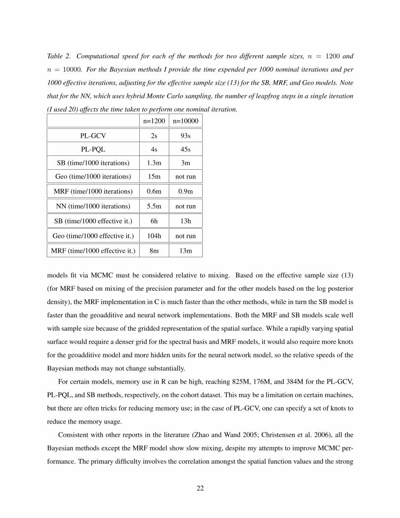
Table 2. Computational speed for each of the methods for two different sample sizes, n = 1200 and

n = 10000. For the Bayesian methods I provide the time expended per 1000 nominal iterations and per

1000 effective iterations, adjusting for the effective sample size (13) for the SB, MRF, and Geo models. Note

that for the NN, which uses hybrid Monte Carlo sampling, the number of leapfrog steps in a single iteration

(I used 20) affects the time taken to perform one nominal iteration.

n=1200 n=10000

PL-GCV 2s 93s

PL-PQL 4s 45s

SB (time/1000 iterations) 1.3m 3m

Geo (time/1000 iterations) 15m not run

MRF (time/1000 iterations) 0.6m 0.9m

NN (time/1000 iterations) 5.5m not run

SB (time/1000 effective it.) 6h 13h

Geo (time/1000 effective it.) 104h not run

MRF (time/1000 effective it.) 8m 13m

models fit via MCMC must be considered relative to mixing. Based on the effective sample size (13)

(for MRF based on mixing of the precision parameter and for the other models based on the log posterior

density), the MRF implementation in C is much faster than the other methods, while in turn the SB model is

faster than the geoadditive and neural network implementations. Both the MRF and SB models scale well

with sample size because of the gridded representation of the spatial surface. While a rapidly varying spatial

surface would require a denser grid for the spectral basis and MRF models, it would also require more knots

for the geoadditive model and more hidden units for the neural network model, so the relative speeds of the

Bayesian methods may not change substantially.

For certain models, memory use in R can be high, reaching 825M, 176M, and 384M for the PL-GCV,

PL-PQL, and SB methods, respectively, on the cohort dataset. This may be a limitation on certain machines,

but there are often tricks for reducing memory use; in the case of PL-GCV, one can specify a set of knots to

reduce the memory usage.

Consistent with other reports in the literature (Zhao and Wand 2005; Christensen et al. 2006), all the

Bayesian methods except the MRF model show slow mixing, despite my attempts to improve MCMC per-

formance. The primary difficulty involves the correlation amongst the spatial function values and the strong

22

relationship between the smoothing parameter(s) and the function values. Based on a long run (100,000 it-

erations) with one data sample from the isotropic dataset, the spectral basis model shows more rapid mixing

of the smoothing parameters than the geoadditive model with effective sample sizes of 772 for σ and 316

for ρ for the spectral basis model compared to 93 for σ for the geoadditive model. In assessing the model

as a whole through the log posterior, the effective sample size for the SB model is 397, somewhat better

than 240 for the geoadditive model. Combined with the speed advantage per nominal iteration of the SB

model, the computational efficiency of the SB model is much better than the geoadditive model. The MRF

sampling scheme involves jointly updating the precision parameter and process values (Knorr-Held and Rue

2002); this approach appears to work very well in this context with an effective sample size of approximately

1600 achieved in only 20,000 iterations. The use of the data augmentation scheme for the probit link may

contribute to this performance; I have not tried the data augmentation approach for the SB or geoadditive

models.

It is difficult to assess the mixing of the neural network model, first because I can only extract the log

likelihood and not the log posterior from the software, and second because the model generally fails to detect

the structure in the data; good mixing for a posterior that doesn’t fit the data is not particularly relevant.

5.3.3 Ease of implementation

The penalized likelihood methods are the easiest to implement in terms of coding and software availability;

both can be fit using R libraries and a few lines of code. The spectral basis and geoadditive models both

require coding an MCMC algorithm, which is relatively complicated, although I provide template code in the

electronic supplement and have posted an R library, spectralGP, that manipulates the spectral representation.

The MRF model used the GMRFLib C library of H. Rue; this was reasonably easy to implement but did

make use of C rather than R, making it somewhat less accessible to users. I have included some basic C code

that does the MCMC, calling GMRFLib as necessary, in the electronic supplement. The FBM software of R.

Neal allows one to fit neural network models without writing code, but the prior specifications are difficult

to understand and wrapper code (e.g., in Matlab or R) is needed to prepare the model and process the final

chain. Also, only certain outputs from the chain are available.

23

6 Case study

6.1 Background and data

The Kaohsiung metropolitan area is a center of petrochemical production in Taiwan. Population density

is high in the vicinity of four petroleum/petrochemical complexes, and data suggest that hydrocarbon and

volatile organic compound concentrations are much higher than in industrialized areas in the United States,

raising concern that the complexes may be causing adverse health effects. In particular, leukemia and

brain cancer have been linked to exposure to pollutants from petrochemical production. A preliminary

unpublished case-control study suggests that individuals less than 30 years old who live within three km

of one of the four complexes have an increase in leukemia and brain neoplasms. An ongoing case-control

investigation is designed to investigate whether proximity to the complexes is linked to leukemia and brain

cancer.

While the actual study is ongoing, I analyze interim data to illustrate the methods. As I need a single

location for each individual, I assigned each individual to the location at which they resided the longest in

the time between birth and diagnosis (diagnosis of the matched case for the controls). I removed individuals

whose location could not be geocoded or was geocoded to the village or district level and those living far

from the center of Kaohsiung city, leaving individuals geocoded to the exact address or to the street of

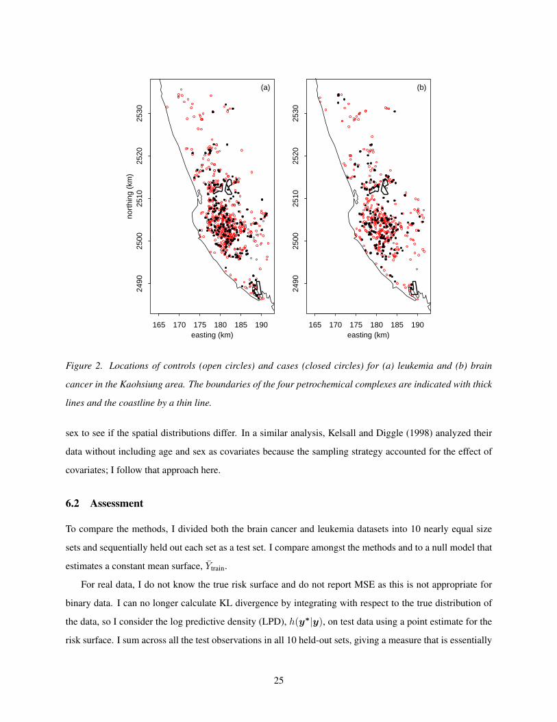
residence. This left 787 (576) individuals in the leukemia (brain cancer) analysis, of whom 206 (165) were

diagnosed with leukemia (brain cancer). The small number of individuals living close to the petrochemical

complexes (Fig. 2) suggests in advance that it will be difficult to detect any increase in risk arising from the

complexes. The sampling of cases finished as of December 2005 and sampling of controls was expected to

finish in August 2006, but because of delays in verifying geocoded addresses I am not able to use the final

cleaned dataset here.

The study was designed to match each case with three controls by date of birth and sex, with controls

chosen from administrative databases. Strictly speaking one should use a conditional likelihood that ac-

counts for the constraint that there is only one case in each matched group; in particular this is important

if matching is done in such a way that the matched controls tend to be close in space to their cases, which

strongly affects the spatial clustering in the resulting dataset (Jarner et al. 2002; Diggle 2003, p. 142). How-

ever, in this situation, matching by date of birth and sex is not expected to cause cases and controls to cluster

tightly. I consider the matching to effectively sample from a control population whose date of birth and

sex distribution closely matches that of the case population. The analysis can then carefully compare the

spatial distributions of cases to this sample from the larger population of individuals of similar birthdate and

24

165 170 175 180 185 190

2490

2500

2510

2520

2530

easting (km)

nort

hing

(km

)

(a)

165 170 175 180 185 190

2490

2500

2510

2520

2530

easting (km)

(b)

Figure 2. Locations of controls (open circles) and cases (closed circles) for (a) leukemia and (b) brain

cancer in the Kaohsiung area. The boundaries of the four petrochemical complexes are indicated with thick

lines and the coastline by a thin line.

sex to see if the spatial distributions differ. In a similar analysis, Kelsall and Diggle (1998) analyzed their

data without including age and sex as covariates because the sampling strategy accounted for the effect of

covariates; I follow that approach here.

6.2 Assessment

To compare the methods, I divided both the brain cancer and leukemia datasets into 10 nearly equal size

sets and sequentially held out each set as a test set. I compare amongst the methods and to a null model that

estimates a constant mean surface, Ytrain.

For real data, I do not know the true risk surface and do not report MSE as this is not appropriate for

binary data. I can no longer calculate KL divergence by integrating with respect to the true distribution of

the data, so I consider the log predictive density (LPD), h(y∗|y), on test data using a point estimate for the

risk surface. I sum across all the test observations in all 10 held-out sets, giving a measure that is essentially

25

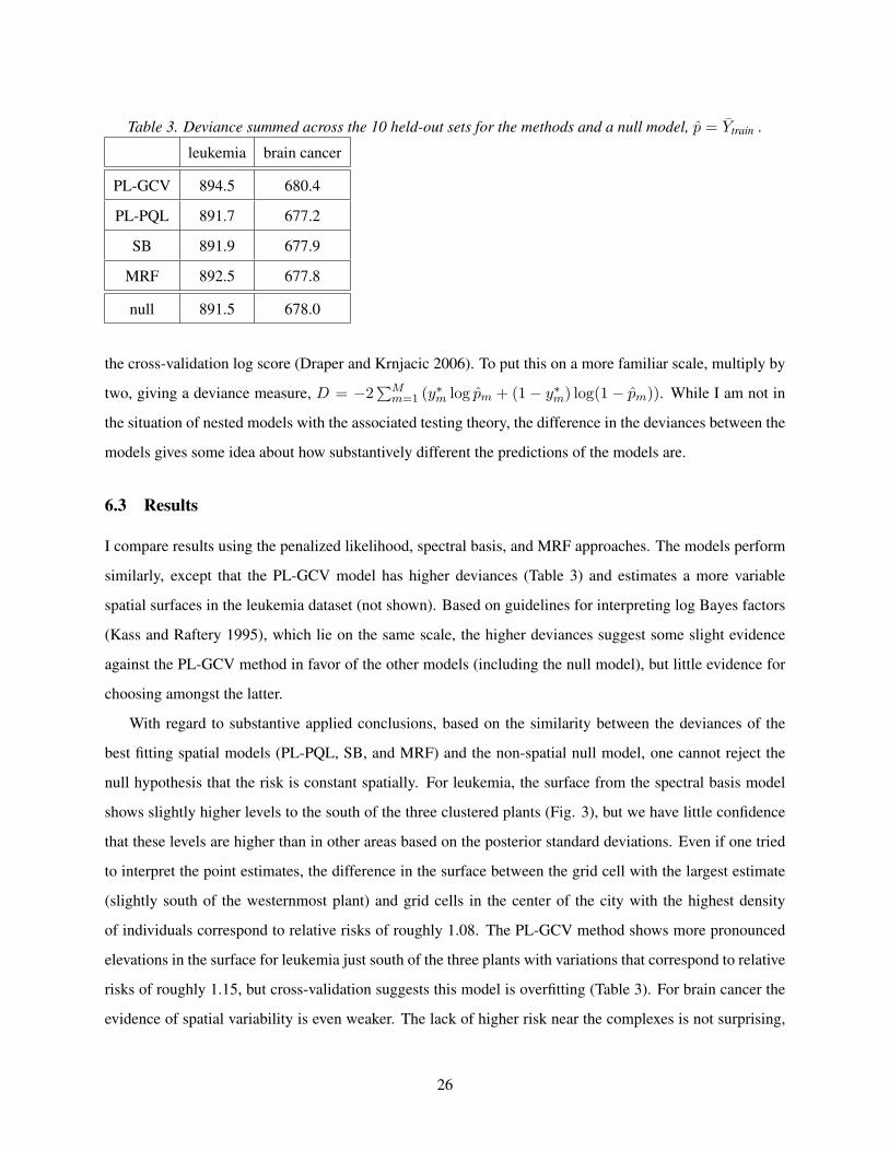
Table 3. Deviance summed across the 10 held-out sets for the methods and a null model, p = Ytrain .

leukemia brain cancer

PL-GCV 894.5 680.4

PL-PQL 891.7 677.2

SB 891.9 677.9

MRF 892.5 677.8

null 891.5 678.0

the cross-validation log score (Draper and Krnjacic 2006). To put this on a more familiar scale, multiply by

two, giving a deviance measure, D = −2∑M

m=1 (y∗m log pm + (1− y∗m) log(1− pm)). While I am not in

the situation of nested models with the associated testing theory, the difference in the deviances between the

models gives some idea about how substantively different the predictions of the models are.

6.3 Results

I compare results using the penalized likelihood, spectral basis, and MRF approaches. The models perform

similarly, except that the PL-GCV model has higher deviances (Table 3) and estimates a more variable

spatial surfaces in the leukemia dataset (not shown). Based on guidelines for interpreting log Bayes factors

(Kass and Raftery 1995), which lie on the same scale, the higher deviances suggest some slight evidence

against the PL-GCV method in favor of the other models (including the null model), but little evidence for

choosing amongst the latter.

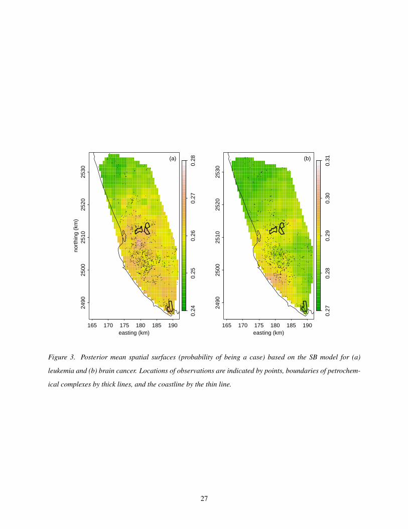
With regard to substantive applied conclusions, based on the similarity between the deviances of the

best fitting spatial models (PL-PQL, SB, and MRF) and the non-spatial null model, one cannot reject the

null hypothesis that the risk is constant spatially. For leukemia, the surface from the spectral basis model

shows slightly higher levels to the south of the three clustered plants (Fig. 3), but we have little confidence

that these levels are higher than in other areas based on the posterior standard deviations. Even if one tried

to interpret the point estimates, the difference in the surface between the grid cell with the largest estimate

(slightly south of the westernmost plant) and grid cells in the center of the city with the highest density

of individuals correspond to relative risks of roughly 1.08. The PL-GCV method shows more pronounced

elevations in the surface for leukemia just south of the three plants with variations that correspond to relative

risks of roughly 1.15, but cross-validation suggests this model is overfitting (Table 3). For brain cancer the

evidence of spatial variability is even weaker. The lack of higher risk near the complexes is not surprising,

26

165 170 175 180 185 190

2490

2500

2510

2520

2530

easting (km)

nort

hing

(km

)

0.24

0.25

0.26

0.27

0.28(a)

165 170 175 180 185 190

2490

2500

2510

2520

2530

easting (km)0.

270.

280.

290.

300.

31(b)

Figure 3. Posterior mean spatial surfaces (probability of being a case) based on the SB model for (a)

leukemia and (b) brain cancer. Locations of observations are indicated by points, boundaries of petrochem-

ical complexes by thick lines, and the coastline by the thin line.

27

because the small number of individuals residing there gives one little power to detect changes in risk there.

Note that this is preliminary analysis and is intended solely as an illustration. However these results and the

limited observations near the complexes suggest the difficulty in detecting spatial patterns from such data.

The overfitting of several methods in the simulations highlight the importance of balancing sensitivity and

specificity and the importance of using methods that achieve this balance. Careful comparison with a null

model can help to avoid overinterpreting point estimates that appear to show spatial variability.

7 Discussion

My simulations suggest that the spectral basis model is the best approach of those considered for fitting

spatial logistic regression models. It provides a good compromise between quality of fit and computational

speed, allowing the user to fit a model in a couple hours, or less time for a basic estimate of the spatial

surface. A disadvantage is the coding effort required, but I provide template code in the electronic supple-

ment and have released an R library, spectralGP. The MRF model as implemented with joint sampling of

hyperparameter and process values and use of sparse matrix algorithms is very fast and mixes very well.

However, point estimation and coverage results for the MRF model were generally not as good as for the

SB model, with poorer performance in terms of the tradeoff between sensitivity and specificity. The MRF

model generally did do as well or better than the penalized likelihood methods, in particular without the

overfitting in the null dataset, and the MRF model can be fit very quickly. If the spectral basis and MRF

models are too slow or too difficult to implement, or show poor mixing for a particular dataset, the penalized

likelihood methods are alternatives but are prone to overfitting.

If computational speed is a concern, one may wish to use one of the penalized likelihood methods

for data exploration and then the spectral basis method to confirm a small number of models. One could

investigate the possibility of overfitting in the penalized likelihood models by comparing different smooth-

ing parameters manually using cross-validation. A potential computational improvement over the spec-

tral basis approach is the MRF approximation to a Gaussian process representation (Rue and Tjelmeland

2002; Rue and Held 2005), which should provide very similar inferential results as to the SB model be-

cause the approach approximates the same underlying GP model. This approach requires the estimation of

appropriately-chosen GMRF precision parameters to mimic the GP, making the implementation involved

(e.g., Rue et al. 2004, Section 4.4). I hope that further software development will make this approach more

easily accessible to users, in which case I expect that this approach will provide an ideal method that is fast

to fit and has the good performance of the GP-based spectral basis approach. Fitting techniques for MRF

28

models that do not require MCMC (Rue and Martino 2006) also appear to be promising, particularly if they

can be implemented for the MRF approximation to a GP.

The methods assessed here are readily generalizable to other non-normal data; I have performed simu-

lations with Poisson-distributed data (a flat function and the multiple extrema function used for the binary

data) and found that the results are similar to those here, with the spectral basis approach outperforming the

other methods (the MRF analysis was not run for the Poisson data). As with binary data, the spectral basis

approach does an excellent job of trading off between sensitivity and specificity, fitting somewhat better

than the other methods on the simulation with a true signal, while avoiding the overfitting that occurs for the

other methods on a null simulation.

The spectral basis model contains an implicit model complexity parameter, the range parameter, which

combined with the multiresolution nature of the basis and the natural penalty on complexity implicit in

the fully Bayesian approach (Denison et al. 2002, p.20) may help explain the superior performance of the

spectral basis model. The multiresolution spectral basis model has basis functions at different frequencies,

and the penalties on the coefficients (through the prior variances) are of different magnitude for the different

frequencies. By estimating the range parameter, in addition to a variance parameter for the basis coefficients,

the model adaptively changes the relative penalties at different frequencies. When the range parameter is

large, the spectral density of the Matérn spatial correlation function produces very small prior variances

for the high-frequency coefficients, essentially zeroing out these coefficients. This has the flavor of L1

penalization, which Grandvalet (1998) has shown to be related to adaptive penalization. This adaptive

penalization may help explain why the SB model does not overfit to the degree that other approaches do.

The natural Bayesian complexity penalty favors large values of this parameter and smoother functions when

that is consistent with the data. Zhang (2004) reports that only the ratio of the variance and range parameters

can be estimated consistently, but I note that in the spectral basis model, the parameters have relatively low

posterior correlation (0.24 in one example), suggesting that both parameters are needed in the model. In

contrast, the PQL version of the penalized likelihood model and its Bayesian implementation have only

a single penalty/variance parameter; smoothing is accomplished by a penalty (the prior in the Bayesian

implementation) on the magnitude of the coefficients, and the same penalty applies to all the coefficients,

whose basis functions lie at the same level of resolution. The penalties on the basis coefficients in smoothing

spline models (which is the form of the GCV penalized likelihood model) change with the frequency of the

corresponding basis functions, but the relative penalties for different frequencies are fixed in advanced rather

than adapting to the data (Brumback and Rice 1998). The MRF model also has a single penalty/variance

parameter, the conditional precision parameter, but the model seems to balance sensitivity and specificity

29

better than the other models with a single such parameter.

All of the methods allow for the inclusion of additional covariates in a linear (xiT β in (1)) or nonpara-

metric fashion (substituting∑

p hp(xi) for xiT β). The spectral basis, geoadditive, and MRF representations

of the spatial surface could also be included as modules in more complicated hierarchical models. These

might be spatial-temporal models, models for multiple outcomes, or models that incorporate deterministic

components. The success of the spectral basis model suggests its promise for use in representing spatial

effects in more complicated models.

My simulations and analysis of the Taiwan data ignore key aspects of spatial case-control data. First,

the spatial logistic regression model does not analyze time to disease onset; spatial survival models such

as that of Li and Ryan (2002) are one approach to this. Second, I assume individuals have fixed locations,

while in reality individuals move over time, affecting their exposure. While a non-spatial model based on

accurate exposure estimates is clearly a better approach than spatial logistic regression, there are reasons a

spatial model may be preferred in certain circumstances. First, exposure estimates are usually very uncertain

and may be unobtainable. The error introduced by assigning individuals to a fixed location may be of less

concern than problems associated with an exposure estimate. Second, even when the spatial structure is

not of primary interest, incorporating a spatial term in a model can be important to control for unmeasured

covariates that may vary spatially. Furthermore, one may be interested in investigating spatial patterns in

health outcomes in an exploratory hypothesis-generating fashion. Ideally, once a spatial pattern of risk is

detected, more detailed investigation of potential risk factors and careful exposure estimation will be done.

Spatial models for binary outcomes have low statistical power, which plagues all of the methods, as can

be seen in the lengths of the confidence and credible intervals. This difficulty arises from fitting a fully

flexible bivariate surface with binary observations, which contain much less information than continuous

or count observations. This is of particular concern for epidemiological data, for which both baseline risks

and relative risks from exposure to disease-causing agents are often small. For cohort data, thousands of

observations are necessary even to estimate simple surfaces with a single peak, such as the simulated dataset

here, while more complicated surfaces, such as risks associated with roadways, would require either many

more observations or very large relative risks from exposure. Even using case-control data with thousands

of observations, the methods have relatively little power with realistic relative risks. When the risk is tied to

a single point source, one might increase power by explicitly including distance to the source in the analysis

(Morris and Wakefield 2000). This could be done by using a parametric risk function based on distance to the

source (Diggle 1990; Lawson 1993) or basing a hypothesis test on distance. However, in many applications

it is unclear what parametric risk function to use because of potentially complicated patterns of exposure;

30

in the Taiwan example, there are four area sources (three of which are clustered) with the exact emission

locations unknown; combined with meteorology this is likely to induce a complicated exposure pattern that

cannot be easily captured with a parametric model. The tradeoff here is between higher power under a good

parametric model and the flexibility and avoidance of parametric assumptions of a nonparametric spatial

representation.

The low power for modelling the bivariate surface also makes it difficult to consider interactions be-

tween space and other covariates. In the Taiwan study, researchers are interested in gene by environment

interactions. For a small number of genotypes, a simple approach would be to fit a separate spatial surface

for each type, but this is unrealistic unless one has a large sample size and a small number of surfaces to

fit. I have little power even without splitting the dataset, particularly given the small number of individuals

residing near the petrochemical complexes.

Because of the low power, I have assessed the methods only on relatively simple surfaces; my most com-

plicated surface has several extrema. The relative success of the methods may change for more complicated

surfaces. With realistic binary epidemiological data, one is unlikely to be able to detect such surfaces, but

in other applications, this may be more realistic.

8 Appendix: Representing functions in the spectral domain

The details in this appendix draw on Dudgeon and Mersereau (1984), Borgman et al. (1984), and Wikle

(2002); a more extensive description is given in Paciorek (2006). The spectral basis approach represents a

function, g(·), on a grid, s#, as a linear combination of orthogonal spectral basis functions, gs# = Zu. The

basis functions represented in the basis matrix, Z, capture behavior at different frequencies, with the most

important basis functions for function estimation being the low-frequency basis functions. The first step in

representing the function is to choose the grid size, Md, in each dimension, d = 1, . . . , D, to be a power of

two. The Md frequencies in the dth dimension are then ωd ∈ 0, 1, . . . , Md2 ,−Md

2 + 1, . . . ,−1, where the

superscript represents the dimension. There is a complex exponential basis function for each distinct vector

of frequencies, (ω1m1

, . . . , ωDmD

), md ∈ 0, . . . ,Md − 1, each with a complex-valued basis coefficient,

um1,...,mD .

First I show how to construct a random, mean zero, Gaussian process in one dimension with domain

(0, 1) from the M spectral coefficients, um = am + bmi, m = 0, . . . ,M − 1, and complex exponential

basis functions, zm(sj) = exp(iωmsj), whose real and imaginary components have frequency ωm. To

approximate real-valued processes, u0, . . . , uM/2 are jointly independent, u0 and uM/2 are real-valued (b0 =

31

bM/2 = 0), and the remaining coefficients are determined, uM/2+1 = uM/2−1, . . . , uM−1 = u1, where the

overbar is the complex conjugate operation. This determinism causes the imaginary components of the basis

functions to cancel, leaving a real-valued process,

g(sj) =M−1∑m=0

zm(sj)um =

M2∑

m=0

exp(iωmsj)(am + bmi) +M−1∑

m=M2

+1

exp(iωmsj)(aM−m − bM−mi)

= 2

a0 +

M2−1∑

m=1

(am cos(ωmsj)− bm sin(ωmsj)) + aM/2 cos(ωM2

sj)

.

Hence for a grid of M values, I approximate the process as a linear combination of M spectral basis func-

tions corresponding to M real-valued sinusoidal basis functions, including the constant function (ω0 = 0).

To approximate mean zero Gaussian processes with a particular stationary covariance function, the co-

efficients have Gaussian prior distributions with mean zero, while the spectral density for the covariance

function, fθ(·), e.g., (6), determines the prior variance of the coefficients: V(um) = fθ(ωm) ⇒ V(a0) =

fθ(ω0); V(aM/2) = fθ(ωM/2); V(am) = V(bm) = 12fθ(ωm), o.w., with the coefficients a priori in-

dependent. The spectral basis construction produces periodic functions (g(0) = g(2π)), so the corre-

lation function of the process on (π, 2π) is the mirror image of the correlation function on (0, π) with

Cor(g(0), g(2π)) = 1. I avoid artifacts from this periodicity by mapping the interval (0, 2π) to (0, 2) and

computing but not using the process values on (1, 2), thereby mapping the original domain of the observa-

tions to (0, 1). Note that the use of πρ rather than ρ in (6) allows one to interpret ρ on the (0, 1) rather than

(0, π) scale. The modelled surface is a piecewise constant surface on an equally-spaced grid of size M/2.

This setup ensures that the correlation structure of the approximating process is close to the correlation

structure of a GP with the desired stationary correlation function.

The setup is similar in two dimensions, with a matrix of coefficients, ((um1,m2)), md ∈ 0, . . . ,Md−1,

and corresponding frequency pairs, (ω1m1

, ω2m2

). As seen in Table 4, many coefficients are again deter-

ministically given by other coefficients to ensure that the process is a linear combination of real-valued

sinusoidal basis functions of varying frequencies and orientations in <2. The real and imaginary com-

ponents of each coefficient, um1,m2 = am1,m2 + bm1,m2i, are again independent with V(am1,m2) =

V(bm1,m2) = 12fθ(ω1

m1, ω2

m2) and for (m1,m2) ∈ (0, 0), (M1

2 , 0), (0, M22 ), (M1

2 , M22 ), bm1,m2 = 0 and

V(am1,m2) = fθ(ω1m1

, ω2m2

). Analogous to the one-dimensional case, I estimate a process on (0, 1)D. To

do so, I map the periodic domain (0, 2π)D to (0, 2)D and then map the observation domain onto the (0, 1)D

portion (maintaining the scale ratio in the different dimensions, unless desired otherwise), again ignoring

the process values outside this region. Note that if the original domain is far from square, I unnecessarily

32

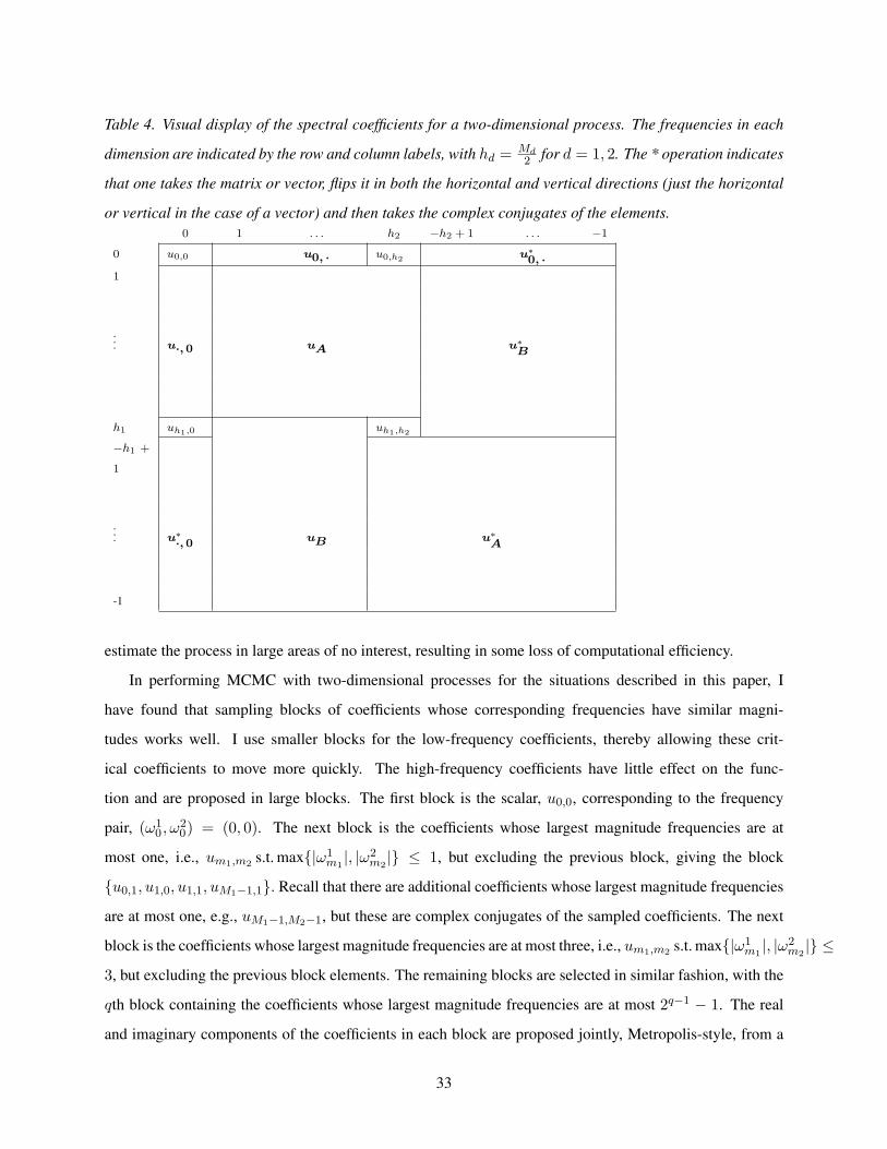
Table 4. Visual display of the spectral coefficients for a two-dimensional process. The frequencies in each

dimension are indicated by the row and column labels, with hd = Md2 for d = 1, 2. The * operation indicates

that one takes the matrix or vector, flips it in both the horizontal and vertical directions (just the horizontal

or vertical in the case of a vector) and then takes the complex conjugates of the elements.0 1 . . . h2 −h2 + 1 . . . −1

0 u0,0 u0, · u0,h2 u∗0, ·

1

... u·, 0 uA u∗B

h1 uh1,0 uh1,h2

−h1 +

1

... u∗·, 0 uB u∗

A

-1

estimate the process in large areas of no interest, resulting in some loss of computational efficiency.

In performing MCMC with two-dimensional processes for the situations described in this paper, I

have found that sampling blocks of coefficients whose corresponding frequencies have similar magni-

tudes works well. I use smaller blocks for the low-frequency coefficients, thereby allowing these crit-

ical coefficients to move more quickly. The high-frequency coefficients have little effect on the func-

tion and are proposed in large blocks. The first block is the scalar, u0,0, corresponding to the frequency

pair, (ω10, ω

20) = (0, 0). The next block is the coefficients whose largest magnitude frequencies are at

most one, i.e., um1,m2 s.t. max|ω1m1|, |ω2

m2| ≤ 1, but excluding the previous block, giving the block

u0,1, u1,0, u1,1, uM1−1,1. Recall that there are additional coefficients whose largest magnitude frequencies

are at most one, e.g., uM1−1,M2−1, but these are complex conjugates of the sampled coefficients. The next

block is the coefficients whose largest magnitude frequencies are at most three, i.e., um1,m2 s.t. max|ω1m1|, |ω2

m2| ≤

3, but excluding the previous block elements. The remaining blocks are selected in similar fashion, with the

qth block containing the coefficients whose largest magnitude frequencies are at most 2q−1 − 1. The real

and imaginary components of the coefficients in each block are proposed jointly, Metropolis-style, from a

33

multivariate normal distribution with independent elements centered on the current values. Since the coef-

ficients have widely-varying scales, I take the proposal variance for each coefficient to be the product of a

tuneable multiplier (one for each block) and the prior variance of the coefficient, which puts the proposal on

the proper scale.

Acknowledgements

The author thanks Louise Ryan for introducing him to the core problem addressed in the paper and for

ongoing advice and suggestions. He also thanks David Schoenfeld for the access to computing resources

necessary for the project and David Christiani, Chu-Ling Yu, and Chen-Yu Liu for the data used in the case

study. The project was supported by grant numbers 5 T32 ES007142-23 (to the Department of Biostatistics

at Harvard School of Public Health) and 5 P30 ES000002 (to Harvard School of Public Health) from the Na-

tional Institute of Environmental Health Sciences (NIEHS), NIH. The contents are solely the responsibility

of the author and do not necessarily represent the official views of NIEHS, NIH.

References

Albert, J. H. and Chib, S. (1993), “Bayesian analysis of binary and polychotomous response data,” Journal

of the American Statistical Association, 88, 669–679.

Banerjee, S., Carlin, B., and Gelfand, A. (2004), Hierarchical modeling and analysis for spatial data:

Chapman & Hall.

Best, N., Arnold, R., Thomas, A., Waller, L., and Conlon, E. (1999), “Bayesian models for spatially

correlated disease and exposure data,” in Bayesian Statistics 6, eds. J. Bernardo, J. Berger, A. Dawid,

and A. Smith, Oxford, U.K.: Oxford University Press, pp. 131–156.

Best, N., Ickstadt, K., and Wolpert, R. L. (2000), “Spatial Poisson regression for health and exposure data

measured at disparate resolutions,” Journal of the American Statistical Association, 95, 1076–1088.

Booth, J. G. and Hobert, J. P. (1999), “Maximizing generalized linear mixed model likelihoods with an

automated Monte Carlo EM algorithm,” Journal of the Royal Statistical Society, Series B, 61, 265–

285.

Borgman, L., Taheri, M., and Hagan, R. (1984), “Three-dimensional, frequency-domain simulations of

34

geological variables,” in Geostatistics for Natural Resources Characterization, Part 1, ed. G. Verly, D.

Reidel Publishing Company, pp. 517–541.

Breslow, N. (2003), “Whither PQL?” Technical Report 192, Department of Biostatistics, University of

Washington.

Breslow, N. E. and Clayton, D. G. (1993), “Approximate inference in generalized linear mixed models,”

Journal of the American Statistical Association, 88, 9–25.

Brumback, B. A. and Rice, J. A. (1998), “Smoothing spline models for the analysis of nested and crossed

samples of curves (C/R: p976-994),” Journal of the American Statistical Association, 93, 961–976.

Carlin, B. P. and Louis, T. A. (2000), Bayes and Empirical Bayes Methods for Data Analysis: Chapman &

Hall Ltd.

Carroll, R., Ruppert, D., and Stefanski, L. (1995), Measurement error in nonlinear models, Boca Raton,

Florida: Chapman & Hall CRC.

Christensen, O. (2004), “Monte Carlo maximum likelihood in model-based geostatistics,” Journal of Com-

putational and Graphical Statistics, 13, 702–718.

Christensen, O., Møller, J., and Waagepetersen, R. (2000), “Analysis of spatial data using generalized

linear mixed models and Langevin-type Markov chain Monte Carlo,” Technical Report R-002009,

Department of Mathematics, Aalborg University.

Christensen, O., Roberts, G., and Sköld, M. (2006), “Robust Markov chain Monte Carlo methods for spatial

generalized linear mixed models,” Journal of Computational and Graphical Statistics, 15, 1–17.

Christensen, O. F. and Waagepetersen, R. (2002), “Bayesian prediction of spatial count data using general-

ized linear mixed models,” Biometrics, 58, 280–286.

Cowles, M. K. and Carlin, B. P. (1996), “Markov chain Monte Carlo convergence diagnostics: A compara-

tive review,” Journal of the American Statistical Association, 91, 883–904.

Cressie, N. (1993), Statistics for Spatial Data (Revised ed.), New York: Wiley-Interscience.

Denison, D. G., Holmes, C. C., Mallick, B. K., and Smith, A. F. M. (2002), Bayesian Methods for Nonlinear

Classification and Regression, New York: Wiley.

Diggle, P. (2003), Statistical Analysis of Spatial Point Patterns (2 ed.), London: Arnold.

35

Diggle, P. J. (1990), “A point process modelling approach to raised incidence of a rare phenomenon in

the vicinity of a prespecified point,” Journal of the Royal Statistical Society, Series A, General, 153,

349–362.

Diggle, P. J., Tawn, J. A., and Moyeed, R. A. (1998), “Model-based geostatistics,” Applied Statistics, 47,

299–326.

Draper, D. and Krnjacic, M. (2006), “Bayesian model specification,” Technical report, Department of

Applied Mathematics and Statistics, University of California Santa Cruz.

Dudgeon, D. and Mersereau, R. (1984), Multidimensional Digital Signal Processing, Englewood Cliffs,

New Jersey: Prentice Hall.

Elliott, P., Wakefield, J., Best, N., and Briggs, D. (2000), “Spatial epidemiology: methods and applications,”

in Spatial epidemiology: methods and applications, eds. P. Elliott, J. Wakefield, N. Best, and D. Briggs,

Oxford University Press, pp. 3–14.

Fahrmeir, L. and Lang, S. (2001), “Bayesian Inference for Generalized Additive Mixed Models Based on

Markov Random Field Priors,” Journal of the Royal Statistical Society C, 50, 201–220.

Gamerman, D. (1997), “Sampling from the posterior distribution in generalized linear mixed models,”

Statistics and Computing, 7, 57–68.

Gelman, A. (2006), “Prior distributions for variance parameters in hierarchical models (comment on article

by Browne and Draper),” Bayesian Analysis, 1(3), 515–534.

Gibbons, R. D. and Hedeker, D. (1997), “Random effects probit and logistic regression models for three-

level data,” Biometrics, 53, 1527–1537.

Grandvalet, Y. (1998), “Least absolute shrinkage is equivalent to quadratic penalization,” in ICANN’98,

Perspectives in Neural Computing, Springer, pp. 201–206.

Green, P. (1995), “Reversible jump Markov chain Monte Carlo computation and Bayesian model determi-

nation,” Biometrika, 82, 711–732.

Greenland, S. (1992), “Divergent biases in ecologic and individual-level studies,” Statistics in Medicine, 11,

1209–1223.

Hastie, T. J. and Tibshirani, R. J. (1990), Generalized Additive Models, London: Chapman & Hall Ltd.

36

Hedeker, D. and Gibbons, R. D. (1994), “A random-effects ordinal regression model for multilevel analysis,”

Biometrics, 50, 933–944.

Higdon, D. (1998), “A process-convolution approach to modeling temperatures in the North Atlantic

Ocean,” Journal of Environmental and Ecological Statistics, 5, 173–190.

Hobert, J. and Wand, M. (2000), “Automatic generalized nonparametric regression via maximum likeli-

hood,” Technical report, Department of Biotatistics, Harvard School of Public Health.

Holmes, C. and Mallick, B. (2003), “Generalized nonlinear modeling with multivariate free-knot regression

splines,” Journal of the American Statistical Association, 98, 352–368.

Hwang, J.-N., Lay, S.-R., Maechler, M., Martin, D., and Schimert, J. (1994), “Regression modeling in back-

propagation and projection pursuit learning,” IEEE Transactions on Neural Networks, 5, 342–353.

Jarner, M. F., Diggle, P., and Chetwynd, A. G. (2002), “Estimation of Spatial Variation in Risk Using

Matched Case-control Data,” Biometrical Journal, 44(8), 936–945.

Kammann, E. and Wand, M. (2003), “Geoadditive models,” Applied Statistics, 52, 1–18.

Kass, R. and Raftery, A. (1995), “Bayes factors,” Journal of the American Statistical Association, 90,

773–795.

Kelsall, J. E. and Diggle, P. J. (1998), “Spatial Variation in Risk of Disease: A Nonparametric Binary

Regression Approach,” Journal of the Royal Statistical Society, Series C: Applied Statistics, 47, 559–

573.

Knorr-Held, L. and Rue, H. (2002), “On Block Updating in Markov Random Field Models for Disease

Mapping,” Scandinavian Journal of Statistics, 29(4), 597–614.

Lawson, A. B. (1993), “On the analysis of mortality events associated with a prespecified fixed point,”

Journal of the Royal Statistical Society, Series A, General, 156, 363–377.

Lee, H. (2004), Bayesian nonparametrics via neural networks: SIAM.

Lenk, P. J. (1999), “Bayesian Inference for Semiparametric Regression Using a Fourier Representation,”

Journal of the Royal Statistical Society, Series B: Statistical Methodology, 61, 863–879.

Li, Y. and Ryan, L. (2002), “Modeling spatial survival data using semi-parametric frailty models,” Biomet-

rics, 58, 287–297.

37

McCulloch, C. E. (1994), “Maximum likelihood variance components estimation for binary data,” Journal

of the American Statistical Association, 89, 330–335.

(1997), “Maximum likelihood algorithms for generalized linear mixed models,” Journal of the

American Statistical Association, 92, 162–170.

Morris, S. and Wakefield, J. (2000), “Assessment of disease risk in relation to a pre-specified source,” in

Spatial epidemiology: methods and applications, eds. P. Elliott, J. Wakefield, N. Best, and D. Briggs,

Oxford University Press, pp. 153–184.

Neal, R. (1993), “Probabilistic Inference Using Markov Chain Monte Carlo Methods,” Technical Report

CRG-TR-93-1, Department of Computer Science, University of Toronto.

(1996), Bayesian Learning for Neural Networks, New York: Springer.

Ngo, L. and Wand, M. (2004), “Smoothing with mixed model software,” Journal of Statistical Software, 9.

Nychka, D. W. (2000), “Spatial-process estimates as smoothers,” in Smoothing and regression: approaches,

computation, and application, ed. M. Schimek, John Wiley & Sons, pp. 393–424.

O’Connell, M. and Wolfinger, R. (1997), “Spatial regression models, response surfaces, and process opti-

mization,” Journal of Computational and Graphical Statistics, 6, 224–241.

Paciorek, C. (2003), Nonstationary Gaussian Processes for Regression and Spatial Modelling, unpublished

Ph.D. dissertation, Carnegie Mellon University, Department of Statistics.

(2006), “Bayesian smoothing of irregularly-spaced data using Fourier basis functions,” Technical

Report 49, Harvard University Biostatistics.

Pan, B., Hong, Y., Chang, G., Wang, M., Cinkotai, F., and Ko, Y. (1994), “Excess cancer mortality among

children and adolescents in residential districts polluted by petrochemical manufacturing plants in Tai-

wan,” Journal of Toxicology and Environmental Health, 43, 117–129.

Prentice, R. L. and Pyke, R. (1979), “Logistic Disease Incidence Models and Case-control Studies,”

Biometrika, 66, 403–412.

Rasmussen, C. E. and Ghahramani, Z. (2002), “Infinite mixtures of Gaussian process experts,” in Advances

in Neural Information Processing Systems 14, eds. T. G. Dietterich, S. Becker, and Z. Ghahramani,

Cambridge, MA: MIT Press.

38

Richardson, S. (1992), “Statistical methods for geographic correlation studies,” in Geographical and envi-

ronmental epidemiology: methods for small-area studies, eds. P. Elliott, J. Cuzick, D. English, and R.

Stern, Oxford University Press, pp. 181–204.

Rue, H. and Held, L. (2005), Gaussian Markov random fields: Theory and applications, Boca Raton:

Chapman & Hall.

Rue, H. and Martino, S. (2006), “Approximate Bayesian inference for hierarchical Gaussian Markov random

fields,” Technical report, Department of Mathematical Sciences, Norwegian University of Science and

Technology.

Rue, H., Steinsland, I., and Erland, S. (2004), “Approximating hidden Gaussian Markov random fields,”

Journal of the Royal Statistical Society, Series B: Statistical Methodology, 66(4), 877–892.

Rue, H. and Tjelmeland, H. (2002), “Fitting Gaussian Markov Random Fields to Gaussian fields,” Scandi-

navian Journal of Statistics, 29(1), 31–49.

Ruppert, D., Wand, M., and Carroll, R. (2003), Semiparametric regression, Cambridge, U.K.: Cambridge

University Press.

Shumway, R. and Stoffer, D. (2000), Time Series Analysis and its Applications, New York: Springer-Verlag.

Wager, C. G., Coull, B. A., and Lange, N. (2004), “Modelling spatial intensity for replicated inhomogeneous

point patterns in brain imaging,” Journal of the Royal Statistical Society, Series B, 66, 429–446.

Wahba, G., Wang, Y., Gu, C., Klein, R., and Klein, B. (1995), “Smoothing spline ANOVA for exponen-

tial families, with application to the Wisconsin Epidemiological Study of Diabetic Retinopathy,” The

Annals of Statistics, 23, 1865–1895.

Waller, L. A., Carlin, B. P., Xia, H., and Gelfand, A. E. (1997), “Hierarchical spatio-temporal mapping of

disease rates,” Journal of the American Statistical Association, 92, 607–617.

Wikle, C. (2002), “Spatial modeling of count data: A case study in modelling breeding bird survey data

on large spatial domains,” in Spatial Cluster Modelling, eds. A. Lawson and D. Denison, Chapman &

Hall, pp. 199–209.

Wolfinger, R. and O’Connell, M. (1993), “Generalized linear mixed models: A pseudo-likelihood ap-

proach,” Journal of Statistical Computation and Simulation, 48, 233–243.

39

Wood, S. (2000), “Modelling and smoothing parameter estimation with multiple quadratic penalties,” Jour-

nal of the Royal Statistical Society, Series B, 62(2), 413–428.

(2003), “Thin plate regression splines,” Journal of the Royal Statistical Society, Series B, 65(1),

95–114.

(2004), “Stable and efficient multiple smoothing parameter estimation for generalized additive

models,” Journal of the American Statistical Association, 99, 673–686.

(2006), Generalized additive models: An introduction with R, Boca Raton: Chapman & Hall.

Wood, S., Jiang, W., and Tanner, M. (2002), “Bayesian mixture of splines for spatially adaptive nonpara-

metric regression,” Biometrika, 89, 513–528.

Zhang, H. (2004), “Inconsistent estimation and asymptotically equal interpolation in model-based geostatis-

tics,” Journal of the American Statistical Association, 99, 250–261.

Zhao, Y. and Wand, M. (2005), “Spatial statistics using general design Bayesian generalized linear mixed

models: some applications,” in submission.

40