Embed Size (px)
Citation preview
COMPUTATIONAL AEROELASTICITY USING A PRESSURE-BASED SOLVER
By
RAMJI KAMAKOTI
A DISSERTATION PRESENTED TO THE GRADUATE SCHOOL OF THE UNIVERSITY OF FLORIDA IN PARTIAL FULFILLMENT
OF THE REQUIREMENTS FOR THE DEGREE OF DOCTOR OF PHILOSOPHY
UNIVERSITY OF FLORIDA
2004

Copyright 2004
by
Ramji Kamakoti

This dissertation is dedicated to my parents and sister.

iv
ACKNOWLEDGMENTS
I would like to express my sincere gratitude to Professor Wei Shyy for his
constant support and guidance throughout this work. Equally, I would like to thank Dr.
Bhavani Sankar, Dr. Andrew Kurdila, Dr. Renwei Mei, Dr. Nagaraj Arakere, and Dr.
Michael Frank for serving on my committee and providing their support in completing
this work. I would like to extend my sincere gratitude to Dr. Siddarth Thakur and other
members of the computational thermo-fluids laboratory for making the work environment
very lively and enjoyable to work in. Lastly, I would like to acknowledge the support
given by my family throughout my career.
v
TABLE OF CONTENTS page ACKNOWLEDGMENTS ................................................................................................. iv
LIST OF TABLES........................................................................................................... viii
LIST OF FIGURES ........................................................................................................... ix
ABSTRACT..................................................................................................................... xiii
CHAPTER
1 INTRODUCTION ...........................................................................................................1
Aeroelasticity and the Fluid-Structure Interaction Problem.........................................1 Problem Statement........................................................................................................4
2 LITERATURE REVIEW ..............................................................................................10
Aerodynamic Models..................................................................................................10 Physical Models...................................................................................................10 Reduced-Order Models .......................................................................................12
Review of Coupled Computational Aeroelasticity (CAE) Models ............................13 Fully coupled Analysis ........................................................................................14 Loosely and Closely Coupled Analysis...............................................................16
Loosely coupled analysis .............................................................................16 Closely coupled analysis ..............................................................................17
Review of Moving Boundary Models ........................................................................22 Review of Geometric Conservation Law ...................................................................24 Review of Interfacing Techniques..............................................................................26
3 GOVERNING EQUATIONS AND OVERVIEW OF ALGORITHM.........................32
Governing Equations ..................................................................................................32 Flow Module .......................................................................................................32
Navier-Stokes equations...............................................................................32 Transformation to curvilinear coordinates ...................................................33
Geometric Conservation Law..............................................................................37 Turbulence Modeling ..........................................................................................38
The k-ε transport equations ..........................................................................40
vi
Filter-based turbulence model for unsteady Reynolds-Averaged Navier-Stokes (RANS) computations .................................................................42
Boundary conditions ....................................................................................43 Wall treatment ..............................................................................................43
Structural Dynamics Model.................................................................................44 Moving Grid Module...........................................................................................48
Overview of Algorithm...............................................................................................50 Discretized Form of Equations............................................................................50 Evaluation of Contravariant velocities on Non-staggered Grid ..........................52 Pressure-Based Flow Solver (Semi-Implicit Method for Pressure-Linked
Equations, SIMPLE) ........................................................................................55 Pressure-Implicit Splitting of Operators (PISO) Algorithm for unsteady
computations ....................................................................................................58 Updating Jacobian values for moving boundary treatment .................................60
First order Implicit Scheme:.........................................................................61 First-order time-averaged scheme:...............................................................62 Second order implicit scheme ......................................................................62 Second order time-averaged evaluation of Jacobian....................................63
Newmark Integration Method for Structure Solver.............................................64 4 COMPUTATIONAL PROCEDURE AND CODE VALIDATION.............................66
Computational Procedure ...........................................................................................66 Geometry definition and Computational Grids ..........................................................67
Geometry Definition............................................................................................67 Computational Grids ...........................................................................................68
Computational fluid dynamic (CFD) grid ....................................................68 Computational structural dynamic (CSD) grid ............................................69
Coupling and Interfacing Procedure ...........................................................................70 Code Validation ..........................................................................................................74
Steady-state CFD Computations .........................................................................75 Unsteady Computations using PISO Algorithm..................................................77
Effect of number of stages on accuracy and stability of PISO algorithm ....80 Momentum Interpolation Techniques for Computing Contravariant Velocities 84 Geometric Conservation Law..............................................................................88
Two-dimensional channel flow: First order backward Euler.......................89 Two-dimensional channel flow: PISO algorithm.........................................94 Three-dimensional elastic wing: AGARD 445.6 .........................................95
Moving Boundary Module ................................................................................100 Structure Solver .................................................................................................102
5 RESULTS AND DISCUSSION..................................................................................105
Coupled Simulation for Incompressible Flow Conditions .......................................105 Comparison of PISO and SIMPLE Algorithms........................................................111 Coupled Simulation for Compressible Flow Conditions..........................................112
vii
Time Scales and Choice of Time Step Size for the Coupled Problem..............113 Flutter Boundary Prediction for AGARD Wing at a Transonic Mach Number116 Flutter Computations Using a Filter-Based Turbulence Model (M=0.96)........124 Summary of Flutter Boundary Prediction for AGARD Wing...........................128
6 CONCLUSIONS AND FUTURE WORK ..................................................................132
Conclusions...............................................................................................................132 Future Directions ......................................................................................................137
LIST OF REFERENCES.................................................................................................138
BIOGRAPHICAL SKETCH ...........................................................................................144
viii
LIST OF TABLES
Table page 2-1. Description and key results of a few fully-coupled analysis methods .......................15
2-2. Description of CAE simulations using CAP-TSD, ENS3DAE and CFL3DAE ........19
2-3. Summary of work with a moving mesh algorithm.....................................................21
2-4. Summary of work related to ALE formulation ..........................................................22
2-5. Comparison of moving mesh algorithms....................................................................24
2-6. Summary of representative interface techniques........................................................28
2-7. Summary of boundary element methods ....................................................................30
4-1. Error Norm versus grid velocity for the four GCL schemes for 3-D wing case using Backward Euler method .................................................................................95
4-2. Error Norm versus grid velocity for the four GCL schemes for 3-D wing case ........98
4-3. Tip deflection at two different time instants for different GCL schemes for 3-D wing case ..................................................................................................................99
4-4. Comparison of wing mode shapes between 10 element beam model (present study) and 120 element plate model.......................................................................102
5-1. Comparison of critical flutter speed and dynamic pressure with experiment and other numerical results ...........................................................................................130
ix
LIST OF FIGURES
Figure page 1-1. Aeroelastic diagram of forces and associated phenomena ...........................................2
1-2. Flutter speed index prediction for AGARD 445.6 wing using several methods..........7
2-1. Sample MDICE environment for aeroelastic simulation ...........................................17
2-2. Coupled fluid-structure flow diagram ........................................................................27
2-3. Varying levels of complexity in modeling for fluids and structures ..........................27
3-1. Displacements Measured with respect to the Elastic Axis ........................................46
3-2. Location of variables u, v and p on a 2-D non-staggered grid for the pressure–based algorithm. .......................................................................................................50
3-3. Overview of the SIMPLE algorithm ..........................................................................58
4-1. Schematic of the AGARD 445.6 wing used in the wind tunnel.................................67
4-2. Overview of the Multi-block CFD grid......................................................................69
4-3. CFD surface grid along with grid distributions at the leading and trailing edges ......69
4-4. Schematic of the FEM grid on the AGARD wing......................................................70
4-5. Schematic to demonstrate interpolation technique.....................................................71
4-6. Schematic of a super element: Portion of the entire structure....................................72
4-7. Sample CFD mesh superimposed on the discretized beam structure.........................73
4-8. Schematic to demonstrate the extrapolation procedure..............................................74
4-9. Top view of the CFD domain showing the type of boundary conditions specified at different surfaces .................................................................................................75
4-10. Steady state surface pressure contours on the AGARD wing ..................................76
x
4-11. Steady state pressure coefficient distribution at different spanwise locations on the top surface ..........................................................................................................76
4-12. Computational domain for flow past square cylinder along with imposed boundary conditions .................................................................................................77
4-13. Periodic oscillation of the cross-stream (v) component of velocity using PISO algorithm for square cylinder case at Re=215..........................................................79
4-14. Vordex shedding past a square cylinder using PISO algorithm for Re=215. A) ∆t=0.001, B) ∆t=0.0005 ...........................................................................................79
4-15. Periodic oscillation of the cross-stream (v) component of velocity using SIMPLE algorithm for square cylinder case at Re=215. .........................................80
4-16. Pressure residual history for unsteady flow over a square cylinder (Re=215).........81
4-17. Periodic oscillation of Cross-stream velocity (v) using different number of stages for PISO algorithm ........................................................................................82
4-18. Computational domain and boundary conditions imposed for flow over a circular cylinder........................................................................................................83
4-19. Pressure residual history for unsteady flow over a circular cylinder (Re=100) .......83
4-20. Periodic oscillation of cross-stream velocity (v) for different number of corrector stages.........................................................................................................84
4-21. Schematic of Cavity flow grid along with boundary conditions ..............................85
4-22. Velocity and pressure contours for cavity flow at Re=100 using different momentum interpolation schemes for various time step sizes at y=0.5 location in the cavity. .............................................................................................................86
4-23. Schematic of computational domain surrounding a cylinder ...................................87
4-24. Velocity and pressure plot for flow around a cylinder at Re=40 using different momentum interpolation schemes for various time step sizes at the symmetry line downstream of the cylinder ...............................................................................88
4-25. Computational grids for channel flow at different time instants ..............................90
4-26. Velocity profile for channel flow with Re=100 at different time instants for coarse grid (151×11) using Backward Euler method...............................................91
4-27. Error norm versus grid velocity using various schemes for channel flow for 151×11 grid using Backward Euler method ............................................................91
xi
4-28. Velocity profile for channel flow with Re=100 at different time instants for fine grid (301×21) using Backward Euler method..........................................................93
4-29. Error norm versus grid velocity using various schemes for channel flow for 301×21 grid using Backward Euler method ............................................................93
4-30. Velocity profile for channel flow at different time instants for 151x11 grid using PISO method ............................................................................................................95
4-31. Plot depicting the arbitrary movement of the wing in the spanwise direction ........97
4-32. Error norm versus grid velocity for the various schemes for AGARD wing using Backward Euler method .................................................................................97
4-33. Spanwise deflection of AGARD wing at four different time instants......................99
4-34. Schematic of multi-block grid used to validate moving mesh module ..................100
4-35. Effect of the 2 parameters, FACMIN and β, on the re-meshing.............................101
4-36. Tip deflection of AGARD wing versus number of time steps for ∆t=0.0001........104
4-37. Tip deflection of AGARD wing versus number of time steps for ∆t=0.001..........104
5-1. Spanwise wing shapes at different time instants (Grid configuration I) ..................106
5-2. Time varying displacement of wing at different spanwise locations (Grid configuration I).......................................................................................................107
5-3. Time history of lift coefficient for AGARD 445.6 wing subject to 1-degree angle of attack for both grid configurations.....................................................................108
5-4. Time history of lift/drag ratio for AGARD 445.6 wing subject to 1-degree angle of attack for both grid configurations. ....................................................................108
5-5. Pressure contour on the surface of the wing at steady state .....................................109
5-6. Comparison of lift coefficient time history for AGARD wing subject to different angles of attack for grid configuration I.................................................................110
5-7. Comparison of lift coefficient time history for AGARD wing subject to different angles of attack for grid configuration I.................................................................110
5-8. Spanwise displacements at three different time instants to compare PISO and SIMPLE methods using incompressible flow around an AGARD wing example at a Re=3.64x10⁵ based on unit root chord. ...........................................................112
5-9. Diffusive and convective time scales near wing tip region for different time step sizes and grids ........................................................................................................114
xii
5-10. Diffusive and convective nondimensional paramter at wing tip spanwise location for different grids and time step sizes ......................................................116
5-11. Generalized displacement versus time for three different dynamic pressures for ∆t=5x10⁻⁵................................................................................................................118
5-12. Generalized displacement versus time for three different dynamic pressures for ∆t=1x10⁻⁵................................................................................................................119
5-13. Effect of grid resolution on generalized displacements using similar CFL numbers ..................................................................................................................120
5-14. Flutter points for different choice of time step sizes (1x10⁻⁵ and 5x10⁻⁵ for grid I (350 K points) and grid configurations (350 K grid and 800 K grid) ....................121
5-15. Tip deflection of wing versus time for grid I (350 K points) using a time step size of 5x10⁻⁵ ..........................................................................................................122
5-16. Wing shapes at maximum and minimum tip deflection points ..............................123
5-17. Mach number contours representing supersonic region in the flow domain at mid-span plane. ......................................................................................................123
5-18. Surface pressure contours indicating supercritical region or region of supersonic flow on the surface of the wing. .............................................................................124
5-19. Blending function plot at mid-span plane...............................................................126
5-20. Comparison of filter-based model and standard k-e model for q/qe=0.98 with ∆t=5x10⁻⁵ and filter size, ∆=0.15. ..........................................................................127
5-21. Flutter boundary comparison between filter-based turbulence model and standard k-ε model using grid I and ∆t=5x10⁻⁵ ......................................................127
5-22. Spanwise wing shape at maximum and minimum tip deflection for (left) M=0.678 and (right) M=1.072 ...............................................................................129
5-23. Mach number contours at maximum and minimum tip deflection points..............129
5-24. Summary of flutter speed index prediction for AGARD 445.6 wing ....................131
xiii
Abstract of Dissertation Presented to the Graduate School of the University of Florida in Partial Fulfillment of the Requirements for the Degree of Doctor of Philosophy
COMPUTATIONAL AEROELASTICITY USING A PRESSURE-BASED SOLVER
By
Ramji Kamakoti
August 2004
Chair: Wei Shyy Major Department: Mechanical and Aerospace Engineering
A computational methodology for performing fluid-structure interaction
computations for three-dimensional elastic wing geometries is presented. The flow solver
used is based on an unsteady Reynolds-Averaged Navier-Stokes (RANS) model. A well-
validated k-ε turbulence model with wall function treatment for near wall region was
used to perform turbulent flow calculations. Relative merits of alternative flow solvers
were investigated. The predictor-corrector-based Pressure Implicit Splitting of Operators
(PISO) algorithm was found to be computationally economic for unsteady flow
computations. Wing structure was modeled using Bernoulli-Euler beam theory. A fully
implicit time-marching scheme (using the Newmark integration method) was used to
integrate the equations of motion for structure. Bilinear interpolation and linear
extrapolation techniques were used to transfer necessary information between fluid and
structure solvers. Geometry deformation was accounted for by using a moving boundary
module. The moving grid capability was based on a master/slave concept and transfinite
xiv
interpolation techniques. Since computations were performed on a moving mesh system,
the geometric conservation law must be preserved. This is achieved by appropriately
evaluating the Jacobian values associated with each cell. Accurate computation of
contravariant velocities for unsteady flows using the momentum interpolation method on
collocated, curvilinear grids was also addressed. Flutter computations were performed for
the AGARD 445.6 wing at subsonic, transonic and supersonic Mach numbers. Unsteady
computations were performed at various dynamic pressures to predict the flutter
boundary. Results showed favorable agreement of experiment and previous numerical
results. The computational methodology exhibited capabilities to predict both qualitative
and quantitative features of aeroelasticity.
1
CHAPTER 1 INTRODUCTION
The term computational aeroelasticity (CAE) generally refers to coupling high-
level computational fluid dynamic (CFD) methods with structural dynamic tools to
perform aeroelastic analysis. Recently, CAE has gained interest as considerable progress
has been made in CFD, computational structural dynamics (CSD), and in computer
technologies. Extensive research on CFD and CSD has already been done. The aim of our
study was to develop a closely coupled CAE model (comprising a detailed CFD model
with a simplified CSD model) to perform fluid-structure interaction computations on
three-dimensional wing bodies.
Aeroelasticity and the Fluid-Structure Interaction Problem
Aeroelasticity can be defined as the phenomena associated with the interaction of
aerodynamic forces and inertial forces within elastic structural systems. There are also
aeroelastic phenomena associated with interaction between aerodynamic and elastic
forces alone (Bisplingoff et al. 1955). Aeroelastic problems mainly arise from the flexible
nature of the structure. In other words, rigid structures do not experience aeroelasticity of
any sort. It is well known that external forces acting on a flexible structural system (such
as a wing) lead to a deformation in the wing geometry, and this structural deformation
thereby leads to additional aerodynamic loads.
2
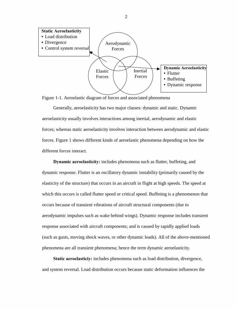
Figure 1-1. Aeroelastic diagram of forces and associated phenomena
Generally, aeroelasticity has two major classes: dynamic and static. Dynamic
aeroelasticity usually involves interactions among inertial, aerodynamic and elastic
forces; whereas static aeroelasticity involves interaction between aerodynamic and elastic
forces. Figure 1 shows different kinds of aeroelastic phenomena depending on how the
different forces interact.
Dynamic aeroelasticity: includes phenomena such as flutter, buffeting, and
dynamic response. Flutter is an oscillatory dynamic instability (primarily caused by the
elasticity of the structure) that occurs in an aircraft in flight at high speeds. The speed at
which this occurs is called flutter speed or critical speed. Buffeting is a phenomenon that
occurs because of transient vibrations of aircraft structural components (due to
aerodynamic impulses such as wake behind wings). Dynamic response includes transient
response associated with aircraft components; and is caused by rapidly applied loads
(such as gusts, moving shock waves, or other dynamic loads). All of the above-mentioned
phenomena are all transient phenomena; hence the term dynamic aeroelasticity.
Static aeroelasticiy: includes phenomena such as load distribution, divergence,
and system reversal. Load distribution occurs because static deformation influences the
AerodynamicForces
Elastic Forces
InertialForces
Static Aeroelasticity • Load distribution • Divergence • Control system reversal
Dynamic Aeroelasticity• Flutter • Buffeting • Dynamic response
3
distribution of aerodynamic pressures over the structure. Divergence is another static
instability (it occurs at a speed called divergence speed) in which the elasticity of the
lifting surface plays a critical role in producing the instability. Another static aeroelastic
phenomenon is control system reversal (it occurs at control reversal speed) in which the
effects of structure displacements are cancelled by elastic deformations of the structure
itself.
Almost every flight vehicle (manned or unmanned) that flies through the
atmosphere undergoes some degree of aeroelasticity. Catastrophic phenomena such as
flutter must be avoided at all costs, and all vehicles must be cleared of such phenomena
before they are put to use. Flight test and wind-tunnel testing are two ways to test for
such phenomena, but they are both expensive and occur late in the design process. Hence,
computational techniques are used first, to assess the aeroelastic characteristics of these
flight vehicles.
While computational methods that study different aspects of aeroelastic response
have been studied for some time, numerous open research issues remain to be resolved.
For example, many approaches in computational aeroelasticity seek to synthesize
independent computational approaches for the aerodynamic and the structural dynamic
subsystems. This strategy is known to be fraught with complications associated with the
interaction between the two simulation modules. Some of the issues arise from the fact
that CFD and CSD mesh systems are quite different. Frequently, the former uses a
Eulerian or spatially fixed-coordinate system, while the latter uses a Lagrangian or
material fixed-coordinate system. Hence, care must be taken to develop a suitable
interfacing technique between the two modules. Also, the time scales can be very
4
different for the two modules, hence one must be careful while performing unsteady
calculations.
There are three major classifications for CAE: fully coupled, closely coupled, and
loosely coupled analyses. In loosely coupled analysis, the fluid and structure modules are
treated as two separate modules, with only external interaction between them. This kind
of methodology can be seen as a multi-disciplinary problem. This method is limited to
small perturbations with moderate linearity. In fully coupled analysis, the governing
equations for fluids and structures are combined into one set of equations, and these
equations are solved and integrated simultaneously. Since the matrices associated with
structures are orders of magnitude stiffer than those associated with fluids, it is virtually
impossible to solve the entire system using a single numerical scheme. Methods have
been developed using fully coupled methods, but they are restricted to two-dimensional
problems and small-scale three-dimensional problems. In the closely coupled approach,
fluids and structures are modeled in separate domains, but are coupled into one module
by an interface technique. The exchange of information between these modules takes
place at the interface or the boundary. The coupling is integrated, thereby allowing the
two modules to exchange information at the boundaries in an efficient manner. Our study
emphasizes this kind of approach.
Problem Statement
The objective of our study was to develop a computational model that is capable of
performing fluid-structure interaction computations on three-dimensional geometries.
Our model was based on a three-dimensional, multi-block, structured CFD solver for the
Navier-Stokes equations. Structural modal dynamic equations were solved
simultaneously and were strongly coupled with the flow equations using fully implicit
5
(iterative) and semi-explicit (non-iterative) time-marching methods. Since the structure
deformation is usually small, a linear structure model was found to be sufficient. To
address the unsteady flow around deforming structures, since the flow can be complex
because of compressibility, existence of shock waves, and effects of viscosity and
turbulence, a more complex model was required. The flow solver addresses the full 3-D
Reynolds-averaged Navier-Stokes (RANS) equations with well-validated turbulence
models. The solver also has the capability to include effects for multi-block moving
boundary treatment. Robust interfacing techniques were also embedded in the coupled
solver to account for transfer of information between the two modules.
Our study aimed to expand a well-validated CFD approach to coupled aeroelastic
models and consider the complexity of coupling procedures in 3-D wing models. A non-
iterative flow solver was used for flow computations, greatly reducing the overall cost of
computations (as the fluids module is the most time consuming among all the modules).
In developing this model, the following issues were addressed:
• efficient moving boundary technique for multi-block structured grids
• preservation of geometric conservation law
• choice of time step of fluid and structure solvers
• accurate computation of contravariant velocities using momentum interpolation method for collocated grids.
The focus of this work was to study the fluid-structure interaction problem for 3-D
wing geometries. The flutter boundary was predicted for a transonic Mach number case.
The AGARD 445.6 wing (Yates 1987) was used to demonstrate the methodology. This
configuration was chosen because extensive research has been done in the field of
aeroelasticity using this model (thus experimental and numerical results are readily
6
available). Several flow solvers, ranging from transonic small disturbance models to full
three-dimensional Navier-Stokes solver and its thin layer approximations have been
coupled to the normal modes of the structure to determine the flutter boundary for the
AGARD wing geometry. Particularly, we are interested in the predicting the transonic dip
observed at transonic mach numbers. This dip is important in determining the minimum
velocity at which flutter can occur across the flight envelope of the vehicle; hence
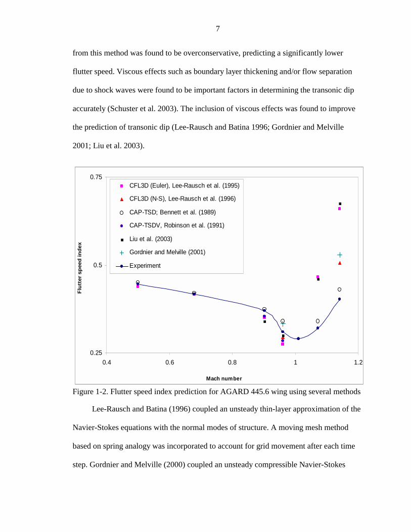
predicting this dip is critical. Figure 1-2 shows the measured and computed flutter
boundary for the AGARD wing using several numerical methods. The solid line
represents the measured flutter boundary originally published by Yates (1963). Both
linear and nonlinear aerodynamic models have been employed to determine the flutter
boundary. Linear analysis using transonic small disturbance model (CAP-TSD; Bennett
et al. 1989) was found to predict the flutter boundaries accurately at subsonic and
supersonic speeds but failed to predict the dip, accurately, at transonic Mach numbers.
Specifically, linear analysis was found to be unconservative in the transonic speed
regime, where it predicted a significantly higher flutter speed. This is attributed to the
highly nonlinear effects arising from formation and disappearance of shock waves at this
Mach number regime as the aircraft undergoes unsteady, flexible motion. Inclusion of
viscous effects to the transonic small disturbance model (CAP-TSDV; Robinson et al.
1991) increased the predictive capability of the model at transonic Mach number, as seen
from the figure. Within nonlinear models, one can use both inviscid as well as viscous
analysis to determine the flutter boundary. The flutter boundary obtained by solving the
unsteady Euler aerodynamics equation of motion coupled to the normal modes of the
structure (CFL3D-Euler; Lee-Rausch and Batina 1995) is shown in Figure 1-2. The result
7
from this method was found to be overconservative, predicting a significantly lower
flutter speed. Viscous effects such as boundary layer thickening and/or flow separation
due to shock waves were found to be important factors in determining the transonic dip
accurately (Schuster et al. 2003). The inclusion of viscous effects was found to improve
the prediction of transonic dip (Lee-Rausch and Batina 1996; Gordnier and Melville
2001; Liu et al. 2003).
Figure 1-2. Flutter speed index prediction for AGARD 445.6 wing using several methods
Lee-Rausch and Batina (1996) coupled an unsteady thin-layer approximation of the
Navier-Stokes equations with the normal modes of structure. A moving mesh method
based on spring analogy was incorporated to account for grid movement after each time
step. Gordnier and Melville (2000) coupled an unsteady compressible Navier-Stokes
0.25
0.5
0.75
0.4 0.6 0.8 1 1.2
Mach number
Flut
ter s
peed
inde
x
CFL3D (Euler), Lee-Rausch et al. (1995)
CFL3D (N-S), Lee-Rausch et al. (1996)
CAP-TSD; Bennett et al. (1989)
CAP-TSDV, Robinson et al. (1991)
Liu et al. (2003)
Gordnier and Melville (2001)
Experiment
8
model with normal modes of structure using a Beam-Warming type implicit time
marching scheme with sub-iterations. An overset grid approach with algebraic mesh
deformation method was used to account for grid movement. The geometric conservation
law, which takes care of certain geometric quantities associated with mesh movement,
was invoked as well. Liu et al. (2003) coupled an unsteady RANS model with normal
modes of structure to predict the flutter boundary for the AGARD wing. Spring analogy
along with transfinite interpolation technique was used to move the multi-block mesh. An
implicit time stepping scheme using sub-iterations was employed to march in time.
Flutter boundary obtained using these methods are summarized in Figure 1-2. Significant
improvement was also seen, while using nonlinear viscous models, at supersonic speed
regimes. Not all of the above-mentioned models incorporated all the features essential in
producing a robust CAE model. Some of the limitations that the previous CAE models
face can be listed as follows
• Fixed-grid computations (Bennett et al. 1989; Robinson et al. 1991) – this is often the case while using transonic small disturbance model
• Use of inviscid flow solvers (Bennett et al. 1989; Lee-Rausch and Batina 1995) – failed to predict viscous effects such as boundary layer growth and/or flow separation
• Implicit time-marching schemes with sub-iterations (Gordnier and Melville 2001; Liu et al. 2003 – being an iterative scheme, it can be computationally expensive. Although such an implicit scheme is unconditionally stable, the choice of time step is limited by the frequency of oscillations of structure.
• Failure to include geometric conservation law (Lee-Rausch and Batina 1995, 1996; Liu et al. 2003)– essential while solving problems on moving mesh systems
We aim at addressing all of the above-mentioned issues and to develop a robust
CAE model capable of predicting the flutter boundary of three-dimensional wing
geometries accurately.

9
A review of the various existing methods in the field of computational
aeroelasticity is given in Chapter 2. The governing equations used by the different models
are addressed in Chapter 3. Chapter 4 discusses the computational procedure and setup
involved with a CAE model. Individual module-validation results along with coupled
simulation results and discussions are given in Chapter 5. Conclusions and thoughts on
future directions are given in Chapter 6.
10
CHAPTER 2 LITERATURE REVIEW
Next we review various aspects and modules related to the field of computational
aeroelasticity (Bennett and Edwards 1998; Friedmann 1999; Huttsell et al. 2001). First,
the various models associated to unsteady aerodynamics are presented. Then we review
various classes of CAE: fully coupled analysis (or unified fluid-structure interaction),
closely coupled aeroelastic analysis, and loosely coupled analysis. We discuss advances
in the field of moving mesh methods for re-meshing purposes and interfacing techniques
for exchanging information between different modules used in some coupled aeroelastic
models. The various formulations of Geometric Conservation Law (GCL) are also
reviewed.
Aerodynamic Models
To understand the fluid-structure interaction problem, we need to model both the
structure and the fluid efficiently. However, since our emphasis was on the fluid (rather
than structure) models, we first review some physical models from the fluids perspective
undergoing time-dependent motion. Different classes of coupled CAE models (explained
earlier) and the issues associated therein are discussed later in this chapter.
Physical Models
Physical models used for treating fluid-structure interaction problems can vary
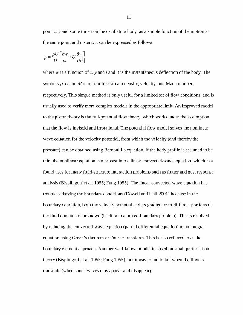
enormously in their complexity, based on the applications. One of the simplest models is
based on piston theory (Dowell and Hall, 2001), which expresses the pressure, p, at some
11
point x, y and some time t on the oscillating body, as a simple function of the motion at
the same point and instant. It can be expressed as follows
U w wp UM t xρ ∂ ∂ = + ∂ ∂
where w is a function of x, y and t and it is the instantaneous deflection of the body. The
symbols ρ, U and M represent free-stream density, velocity, and Mach number,
respectively. This simple method is only useful for a limited set of flow conditions, and is
usually used to verify more complex models in the appropriate limit. An improved model
to the piston theory is the full-potential flow theory, which works under the assumption
that the flow is inviscid and irrotational. The potential flow model solves the nonlinear
wave equation for the velocity potential, from which the velocity (and thereby the
pressure) can be obtained using Bernoulli’s equation. If the body profile is assumed to be
thin, the nonlinear equation can be cast into a linear convected-wave equation, which has
found uses for many fluid-structure interaction problems such as flutter and gust response
analysis (Bisplingoff et al. 1955; Fung 1955). The linear convected-wave equation has
trouble satisfying the boundary conditions (Dowell and Hall 2001) because in the
boundary condition, both the velocity potential and its gradient over different portions of
the fluid domain are unknown (leading to a mixed-boundary problem). This is resolved
by reducing the convected-wave equation (partial differential equation) to an integral
equation using Green’s theorem or Fourier transform. This is also referred to as the
boundary element approach. Another well-known model is based on small perturbation
theory (Bisplingoff et al. 1955; Fung 1955), but it was found to fail when the flow is
transonic (when shock waves may appear and disappear).
12
Another class of models is the time-linearized or dynamically linear model, in
which a steady-state nonlinear solution is used as a starting point; then a small dynamic
perturbation about this steady flow is considered, and all subsequent flow variables and
shock motion are assumed to vary in a linear fashion. This model leads to an order of
magnitude reduction in computer resources compared to the nonlinear model, and was
found to be sufficient for many problems. However, this method was found to be less
useful for turbomachinery problems. This approach can be extended to determine a full
dynamically nonlinear solution, which involves solving a nonlinear convected-wave
equation for potential flow or Euler or Navier-Stokes models. Either finite-difference or
finite-volume schemes in spatial variables can be used to convert the system of partial
difference equations to ordinary differential equations, which forms the basis for CFD.
Additional models must be developed to account for turbulence flow features, and for
transition from laminar to turbulent flows. Another class of models beginning to gain
interest in the field of fluid-structure interaction is reduced-order modeling (ROM)
techniques, discussed next.
Reduced-Order Models
For the past several decades, researchers have worked in the field of CFD to
develop models for complex unsteady flows. The computational cost for high
dimensionality model, especially for aeroelastic problems, has limited the use of full CFD
models for such applications. Recently, advances are being made to develop a novel
technique for unsteady flows based on the modal character of flows, which can be termed
reduced-order models. In the structural dynamics world, over the years, finite element
models for structural dynamics have been reduced in size by using the normal or
eigenmodes of the structure, thereby reducing the model to a few degrees of freedom
13
from thousands of degrees of freedom (Dowell and Hall 2001). This reduces the
computation time for solving such problems, while maintaining the accuracy of the
physical phenomena. This method has also gained interest in the field of fluid dynamics,
because such an approach gives us great benefits (saving computational costs and giving
insight into the dynamics of the fluid models by considering their different modal
structures). This method involves constructing a computational aerodynamic model
using the dominant eigenmodes of unsteady aerodynamic flows. Combining such a
reduced-order aerodynamic model with a structural modal model is an efficient way to
form an aeroelastic modal model with a modest number of degrees of freedom.
Extracting the dominant eigenmodes for large dimensional systems can be potentially
difficult. Hence another modal approach that seeks to include more information on the
flow response to enhance the accuracy of the reduced model has been developed and it is
called the proper orthogonal decomposition (POD) method (Ahlman et al. 2002; Zhang et
al. 2003). It is a much simpler approach than the eigenmode approach, and it uses a
methodology based on nonlinear dynamics and signal processing. One disadvantage of
this method is that determining the POD modes can be computationally expensive
compared to determining the eigenmodes. Extensive research is being done to construct
nonlinear aerodynamic ROMs and to use the eigenmode ROM approach to develop better
turbulence models. However, it is still unknown whether ROM or POD approach can
accurately predict all the length scales associated with the turbulence models.
Review of Coupled CAE Models
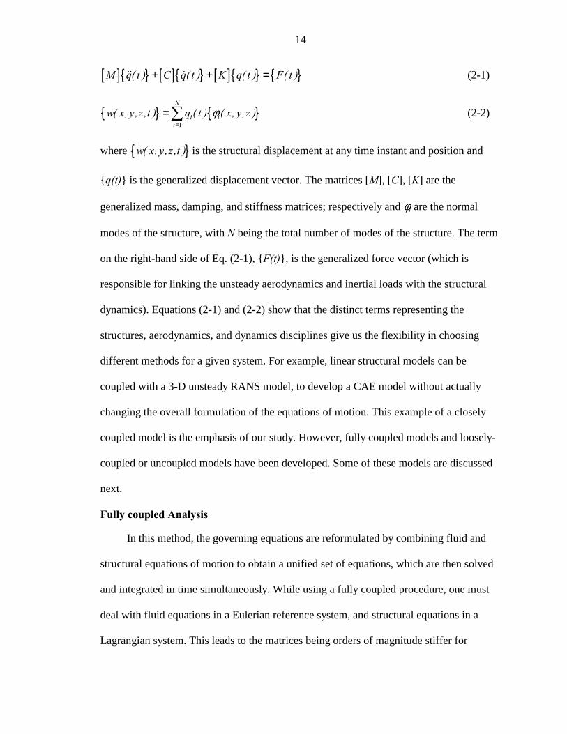
Before looking at the various CAE models, the generalized equations of motion
(Schuster et al. 2003) are given to explain CAE methodologies
14
[ ] [ ] [ ] M q( t ) C q( t ) K q( t ) F( t )+ + =!! ! (2-1)
1
N
i ii
w( x, y,z,t ) q ( t ) ( x, y,z )φ=
=∑ (2-2)
where w( x, y,z,t ) is the structural displacement at any time instant and position and
q(t) is the generalized displacement vector. The matrices [M], [C], [K] are the
generalized mass, damping, and stiffness matrices; respectively and φi are the normal
modes of the structure, with N being the total number of modes of the structure. The term
on the right-hand side of Eq. (2-1), F(t), is the generalized force vector (which is
responsible for linking the unsteady aerodynamics and inertial loads with the structural
dynamics). Equations (2-1) and (2-2) show that the distinct terms representing the
structures, aerodynamics, and dynamics disciplines give us the flexibility in choosing
different methods for a given system. For example, linear structural models can be
coupled with a 3-D unsteady RANS model, to develop a CAE model without actually
changing the overall formulation of the equations of motion. This example of a closely
coupled model is the emphasis of our study. However, fully coupled models and loosely-
coupled or uncoupled models have been developed. Some of these models are discussed
next.
Fully coupled Analysis
In this method, the governing equations are reformulated by combining fluid and
structural equations of motion to obtain a unified set of equations, which are then solved
and integrated in time simultaneously. While using a fully coupled procedure, one must
deal with fluid equations in a Eulerian reference system, and structural equations in a
Lagrangian system. This leads to the matrices being orders of magnitude stiffer for
15
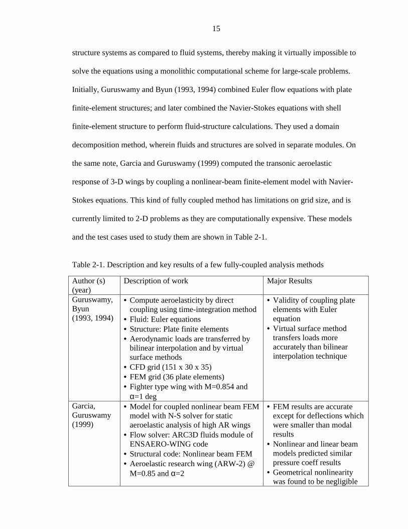
structure systems as compared to fluid systems, thereby making it virtually impossible to
solve the equations using a monolithic computational scheme for large-scale problems.
Initially, Guruswamy and Byun (1993, 1994) combined Euler flow equations with plate
finite-element structures; and later combined the Navier-Stokes equations with shell
finite-element structure to perform fluid-structure calculations. They used a domain
decomposition method, wherein fluids and structures are solved in separate modules. On
the same note, Garcia and Guruswamy (1999) computed the transonic aeroelastic
response of 3-D wings by coupling a nonlinear-beam finite-element model with Navier-
Stokes equations. This kind of fully coupled method has limitations on grid size, and is
currently limited to 2-D problems as they are computationally expensive. These models
and the test cases used to study them are shown in Table 2-1.
Table 2-1. Description and key results of a few fully-coupled analysis methods
Author (s) (year)
Description of work Major Results
Guruswamy, Byun (1993, 1994)
• Compute aeroelasticity by direct coupling using time-integration method
• Fluid: Euler equations • Structure: Plate finite elements • Aerodynamic loads are transferred by
bilinear interpolation and by virtual surface methods
• CFD grid (151 x 30 x 35) • FEM grid (36 plate elements) • Fighter type wing with M=0.854 and
α=1 deg
• Validity of coupling plate elements with Euler equation
• Virtual surface method transfers loads more accurately than bilinear interpolation technique
Garcia, Guruswamy (1999)
• Model for coupled nonlinear beam FEM model with N-S solver for static aeroelastic analysis of high AR wings
• Flow solver: ARC3D fluids module of ENSAERO-WING code
• Structural code: Nonlinear beam FEM • Aeroelastic research wing (ARW-2) @
M=0.85 and α=2
• FEM results are accurate except for deflections which were smaller than modal results
• Nonlinear and linear beam models predicted similar pressure coeff results
• Geometrical nonlinearity was found to be negligible

16
Loosely and Closely Coupled Analysis
In this class of methodologies, unlike the fully coupled analysis, the structural and
fluid equations are solved using two separate solvers. This can result in two different
computational grids (structured or unstructured), which are not likely to coincide at the
boundary. This calls for an interfacing technique to be developed, to exchange
information back and forth between the two modules. This is true for both loosely and
closely coupled approaches. We now review each of these methods separately.
Loosely coupled analysis
The loosely coupled approach has only external interaction between the fluid and
structure modules; or the information is exchanged after partial or complete convergence
(Smith et al. 1996a). This approach is like a multidisciplinary computing environment
(MDICE) (Seigel et al. 1998), where one effectively controls the interaction between two
commercial codes for each of the modules by means of interfacing techniques. This gives
us the flexibility of choosing different solvers for each of the modules but the coupling
procedure loses accuracy as the modules are updated only after partial or complete
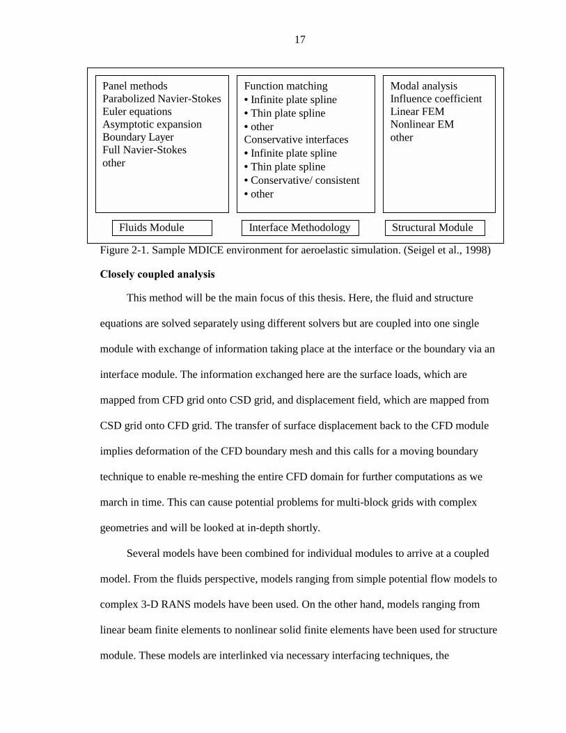
convergence. A typical block diagram of MDICE is shown in Figure 2-1. Here, the
interface methodology has been divided into two categories: function matching interface
and conservative interface. Function matching interfaces provide the closest match
between data on the two computational grids. Conservative interfaces aim at conserving
relevant properties (such as forces and momentum) during the transfer process.
17
Figure 2-1. Sample MDICE environment for aeroelastic simulation. (Seigel et al., 1998)
Closely coupled analysis
This method will be the main focus of this thesis. Here, the fluid and structure
equations are solved separately using different solvers but are coupled into one single
module with exchange of information taking place at the interface or the boundary via an
interface module. The information exchanged here are the surface loads, which are
mapped from CFD grid onto CSD grid, and displacement field, which are mapped from
CSD grid onto CFD grid. The transfer of surface displacement back to the CFD module
implies deformation of the CFD boundary mesh and this calls for a moving boundary
technique to enable re-meshing the entire CFD domain for further computations as we
march in time. This can cause potential problems for multi-block grids with complex
geometries and will be looked at in-depth shortly.
Several models have been combined for individual modules to arrive at a coupled
model. From the fluids perspective, models ranging from simple potential flow models to
complex 3-D RANS models have been used. On the other hand, models ranging from
linear beam finite elements to nonlinear solid finite elements have been used for structure
module. These models are interlinked via necessary interfacing techniques, the
Panel methods Parabolized Navier-Stokes Euler equations Asymptotic expansion Boundary Layer Full Navier-Stokes other
Function matching • Infinite plate spline • Thin plate spline • other Conservative interfaces • Infinite plate spline • Thin plate spline • Conservative/ consistent • other
Modal analysis Influence coefficient Linear FEM Nonlinear EM other
Fluids Module Interface Methodology Structural Module
18
complexity of which depends on what two models are used for the individual modules. A
brief summary of some of the models that have been developed in the past will be shown
next.
Cunningham et al. (1988) developed a computational scheme to perform transonic
aeroelastic analysis by coupling transonic small disturbance (TSD) potential flow
equations (CAP-TSD) with the natural vibrational modes of the structure. Viscous effects
were later incorporated into the flow solver by including an inverse integral boundary
layer model. The equations of motion were solved on a sheared cartesian grid where the
lifting surfaces were modeled as thin plates. This kind of approach simplified the task of
generating grids and no moving boundary algorithm was required as the surface velocity
boundary condition was applied at a mean plane. This technique of using TSD
formulation failed in the presence of a strong shock or when viscous effects are
dominant.
To overcome this, Schuster et al. (1990) came up with a model that uses a 3-D flow
solver coupled with a linear structure model to study the aeroelastic analysis of a fighter
aircraft (ENS3DAE). Thin layer approximations to the full three-dimensional
compressible RANS equations were used. A three-dimensional implementation of the
Beam-Warming implicit scheme was employed for temporal integration. The equations
were solved on multi-block curvilinear grids. The linear generalized mode shapes were
used to model the structure. A grid motion algorithm that uses an algebraic shearing
technique was used to account for the grid movement.
A similar method (CFL3DAE), developed by Lee-Rausch and Batina (1995, 1996),
couples a linear, normal mode structural dynamics model with the thin-layer three-

19
dimensional compressible RANS model. Time marching was accomplished by means of
a second order accurate backward time differencing scheme. A pseudo time sub-iteration
method was introduced to expedite the convergence at each time step. A moving mesh
algorithm based on spring analogy was used here. This model was used to predict the
wing flutter boundary. An overview of the above-mentioned models, namely, CAP-TSD,
ENS3DAE and CFL3DAE, have been given by Bennett and Edwards (1998) and Huttsell
et al. (2001). The main features and results of these methods are shown in Table 2-2.
Table 2-2. Description of CAE simulations using CAP-TSD, ENS3DAE and CFL3DAE Author (s) (year)
Description of work Major Results
Cunningham, Batina, Bennett (1988)
• Computational scheme for transonic aeroelastic analysis to perform flutter analysis
• Flow: Transonic small disturbance formulation
• Structure: Lagrange Equations of motion based on the natural vibrational modes
• AGARD configuration with 45 deg sweep angle and M=0.338-1.141
• Aerodynamic forces and flutter characteristics obtained using linear formulation compared well with expt.
• Non-linear flutter results compared well with expt but not so with linear results
• Can treat configurations with arbitrary lifting surfaces
Lewis and Smith (1998)
• External aeroelastic simulation for internal aerodynamics and shell structures
• Flow: ENS3D • Predictor-corrector scheme for structural
integration • Tested on an engine liner to study flutter
with M=0.7 in inner region and M=0.4 in the annular region
• Results showed the engine liner to be dynamically stable
• Inner flow Mach no. had little effect on aeroelastic response
• Effect of pressure loadings on the shell structures were not considered in this method
20
Table 2-2. Continued Author (s) (year)
Description of work Major Results
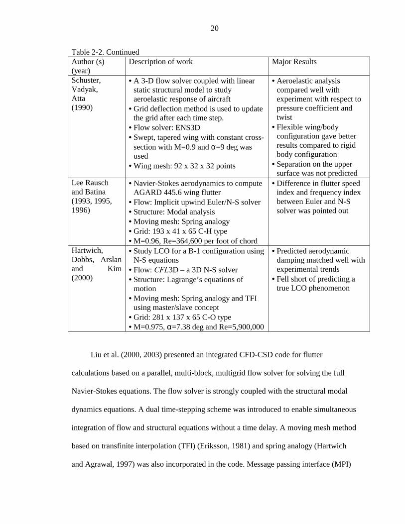
Schuster, Vadyak, Atta (1990)
• A 3-D flow solver coupled with linear static structural model to study aeroelastic response of aircraft
• Grid deflection method is used to update the grid after each time step.
• Flow solver: ENS3D • Swept, tapered wing with constant cross-
section with M=0.9 and α=9 deg was used
• Wing mesh: 92 x 32 x 32 points
• Aeroelastic analysis compared well with experiment with respect to pressure coefficient and twist
• Flexible wing/body configuration gave better results compared to rigid body configuration
• Separation on the upper surface was not predicted
Lee Rausch and Batina (1993, 1995, 1996)
• Navier-Stokes aerodynamics to compute AGARD 445.6 wing flutter
• Flow: Implicit upwind Euler/N-S solver • Structure: Modal analysis • Moving mesh: Spring analogy • Grid: 193 x 41 x 65 C-H type • M=0.96, Re=364,600 per foot of chord
• Difference in flutter speed index and frequency index between Euler and N-S solver was pointed out
Hartwich, Dobbs, Arslan and Kim (2000)
• Study LCO for a B-1 configuration using N-S equations
• Flow: CFL3D – a 3D N-S solver • Structure: Lagrange’s equations of
motion • Moving mesh: Spring analogy and TFI
using master/slave concept • Grid: 281 x 137 x 65 C-O type • M=0.975, α=7.38 deg and Re=5,900,000
• Predicted aerodynamic damping matched well with experimental trends
• Fell short of predicting a true LCO phenomenon
Liu et al. (2000, 2003) presented an integrated CFD-CSD code for flutter
calculations based on a parallel, multi-block, multigrid flow solver for solving the full
Navier-Stokes equations. The flow solver is strongly coupled with the structural modal
dynamics equations. A dual time-stepping scheme was introduced to enable simultaneous
integration of flow and structural equations without a time delay. A moving mesh method
based on transfinite interpolation (TFI) (Eriksson, 1981) and spring analogy (Hartwich
and Agrawal, 1997) was also incorporated in the code. Message passing interface (MPI)
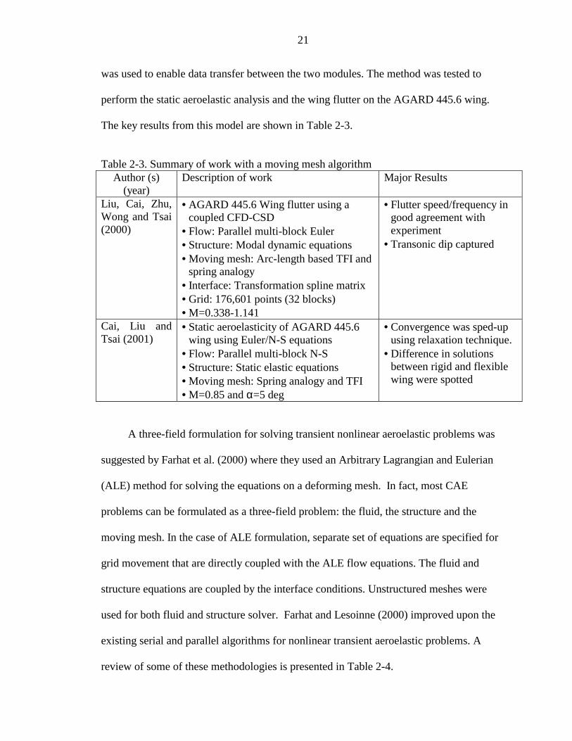
21
was used to enable data transfer between the two modules. The method was tested to
perform the static aeroelastic analysis and the wing flutter on the AGARD 445.6 wing.
The key results from this model are shown in Table 2-3.
Table 2-3. Summary of work with a moving mesh algorithm
Author (s) (year)
Description of work Major Results
Liu, Cai, Zhu, Wong and Tsai (2000)
• AGARD 445.6 Wing flutter using a coupled CFD-CSD
• Flow: Parallel multi-block Euler • Structure: Modal dynamic equations • Moving mesh: Arc-length based TFI and
spring analogy • Interface: Transformation spline matrix • Grid: 176,601 points (32 blocks) • M=0.338-1.141
• Flutter speed/frequency in good agreement with experiment
• Transonic dip captured
Cai, Liu and Tsai (2001)
• Static aeroelasticity of AGARD 445.6 wing using Euler/N-S equations
• Flow: Parallel multi-block N-S • Structure: Static elastic equations • Moving mesh: Spring analogy and TFI • M=0.85 and α=5 deg
• Convergence was sped-up using relaxation technique.
• Difference in solutions between rigid and flexible wing were spotted
A three-field formulation for solving transient nonlinear aeroelastic problems was
suggested by Farhat et al. (2000) where they used an Arbitrary Lagrangian and Eulerian
(ALE) method for solving the equations on a deforming mesh. In fact, most CAE
problems can be formulated as a three-field problem: the fluid, the structure and the
moving mesh. In the case of ALE formulation, separate set of equations are specified for
grid movement that are directly coupled with the ALE flow equations. The fluid and
structure equations are coupled by the interface conditions. Unstructured meshes were
used for both fluid and structure solver. Farhat and Lesoinne (2000) improved upon the
existing serial and parallel algorithms for nonlinear transient aeroelastic problems. A
review of some of these methodologies is presented in Table 2-4.

22
Table 2-4. Summary of work related to ALE formulation Author (s) (year)
Description of work Major Results
Farhat, Pierson and Degand (2000)
• Computational method to simulate transient aeroelastic response of flexible aircraft during high-G maneuvers
• Flow: Arbitrary Lagrangian-Euler equations are incorporated into the unstructured flow solver (Euler)
• Structure: Corotational formulation • M=0.901 and α=1 deg on Langley
fighter
• Qualitative validation of results was done
• Geometric conservation law was incorporated
• Viscous effects were neglected
Farhat and Lesoinne (2000)
• Serial and Parallel methodologies for nonlinear transient aeroelastic problems
• Flow: ALE formulation • Moving mesh: Dynamic mesh equations
coupled with the flow equations • M=0.901 on an AGARD 445.6 wing
• Partitioned algorithms were found to be efficient than monolithic schemes
Geuzine, Brown and Farhat (2002)
• Three-field formulation for flutter analysis of F-16 configuration
• Flow: ALE formulation • Structure: Elastodynamic equations • Moving mesh: Dynamic mesh equations
combined with flow eqns. • M=0.7-1.4 on F-16 wing • Grid size: 403,919 (63,044 on wing
surface)
• Energy conservative exchange of aerodynamic and elastodynamic data was shown
• Method was found to be effective in the transonic regime and not as effective in the subsonic and supersonic regime
Review of Moving Boundary Models
Having reviewed the various developments in the field of computational
aeroelasticity as far as coupling procedure, our focus shift towards one of the most key
aspects of computational aeroelasticty, which is the deforming mesh method. Since the
structure movement needs to be accounted for in the fluid domain, we need to ensure that
the entire flow domain is re-meshed appropriately. Also, an efficient moving boundary
module is very important for performing unsteady flow calculations such as flutter
simulation of wings and turbo-machinery blades. Since the grid needs to be updated
frequently in unsteady computations, a fast and automatic grid deformation procedure is
23
an essential feature. Several models have been developed over the past decade and we
will review some of the methods in this section and point out the advantages and
disadvantages, if any.
Initially, a spring analogy method, originally proposed by Batina (1989) for
unstructured grids and later expanded by Robinson et al. (1991) to structured grids, was
used to generate dynamic grids for structured and unstructured solvers. This method can
handle large deformations but, being an iterative method resembling an elliptic grid
generator, it was found to be computational expensive for larger grid sizes.
Schuster et al. (1990) and Bhardwaj et al. (1998) used a simple algebraic shearing
technique to deform the grid by redistributing the grid points along grid lines that are in
the direction normal to the surface. This method can cause potential problems when the
geometry becomes complex when it becomes difficult to locate the radial direction
normal to the surface. Also, this method is limited to small deformations and large
deformations may lead to poor grid quality and crossover of grid lines.
A transfinite interpolation (TFI) method (Eriksson, 1982) is typically used for
regenerating individual blocks in multi-block meshes. Hartwich and Agrawal (1997)
combined the spring analogy method with the TFI method for regenerating multi-block
grids. Spring analogy was used to move the boundary edges of the blocks whereas TFI
was used to re-mesh the surface and interior volume of each block. A point-by-point
match was enforced between two abutting blocks. Potsdam and Guruswamy (2001)
improved the above method and incorporated parallelization for mesh regeneration.
Another class of methods for re-meshing purposes is solving the moving mesh
partial differential equations (Huang et al., 1994; Huang and Russell, 1999; Huang,
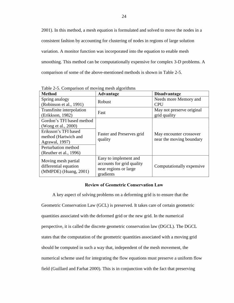
24
2001). In this method, a mesh equation is formulated and solved to move the nodes in a
consistent fashion by accounting for clustering of nodes in regions of large solution
variation. A monitor function was incorporated into the equation to enable mesh
smoothing. This method can be computationally expensive for complex 3-D problems. A
comparison of some of the above-mentioned methods is shown in Table 2-5.
Table 2-5. Comparison of moving mesh algorithms Method Advantage Disadvantage Spring analogy (Robinson et al., 1991) Robust Needs more Memory and
CPU Transfinite interpolation (Erikkson, 1982) Fast May not preserve original
grid quality Gordon’s TFI based method (Wong et al., 2000) Eriksson’s TFI based method (Hartwich and Agrawal, 1997) Perturbation method (Reuther et al., 1996)
Faster and Preserves grid quality
May encounter crossover near the moving boundary
Moving mesh partial differential equation (MMPDE) (Huang, 2001)
Easy to implement and accounts for grid quality near regions or large gradients
Computationally expensive
Review of Geometric Conservation Law
A key aspect of solving problems on a deforming grid is to ensure that the
Geometric Conservation Law (GCL) is preserved. It takes care of certain geometric
quantities associated with the deformed grid or the new grid. In the numerical
perspective, it is called the discrete geometric conservation law (DGCL). The DGCL
states that the computation of the geometric quantities associated with a moving grid
should be computed in such a way that, independent of the mesh movement, the
numerical scheme used for integrating the flow equations must preserve a uniform flow
field (Guillard and Farhat 2000). This is in conjunction with the fact that preserving
25
uniform field implies first order accuracy. In addition, Guillard and Farhat (2000) showed
that for a p-order time-accurate scheme on a fixed mesh, satisfying the corresponding p-
order DGCL is a sufficient condition for the scheme to be at least first order time
accurate on a moving mesh. They established the requirement that preserving the uniform
flow field on moving grids is related to a consistency condition. It has also been proven
that not satisfying the DGCL introduces a weak instability in the numerical solution on
moving grids (Lesoinne and Farhat, 1996).
Substantial evidence exists showing that not satisfying the geometric conservation
law leads to erroneous solutions or spurious oscillations in the solution (Guillard and
Farhat 2000; Lesoinne and Farhat, 1996; Farhat et al., 2001 & 2003). For example, Shyy
et al. (1996) demonstrated that without explicitly enforcing GCL, O(1) error could be
induced in the computation simply due to the grid movement effect. It has also been
shown that satisfying the DGCL can improve the time-accuracy of computations on
moving grids (Koobus and Farhat, 1999). One of the widely used methods for fluid-
structure interaction problems is the ALE formulation. It formulates the Navier-Stokes
equations in three co-ordinate systems namely, material or Lagrangian (for structure
motion), spatial or Eulerian (for fluid motion) and referential (for grid movement). Farhat
et al. (2001, 2003) showed that for ALE schemes, satisfying the DGCL leads to a
necessary and sufficient condition for the numerical scheme to preserve non-linear
stability on a fixed grid. However, there have been a few cases where satisfying or not
satisfying the GCL produced the same results (Morton et al., 1998).
It should be noted that since GCL arises due to the numerical procedures devised
based on grid movement, its implications are expected to be scheme dependent.
26
Alternative forms of the GCL have been implemented over the years to study its impact
on solution accuracy. Thomas and Lombard (1979) implemented the GCL for density-
based finite difference schemes on structured meshes by updating the value of the
Jacobian at each time step. Shyy et al. (1996, 2001) implemented the GCL along the lines
of Thomas and Lombard for pressure-based finite volume schemes by updating the
Jacobian values after every time step using a first order backward Euler time-integration
scheme. Lesoinne and Farhat (1996) developed a first order, time accurate scheme
preserving the GCL using the density-based ALE finite volume as well as finite element
schemes on unstructured grids. Koobus and Farhat (1999) proposed a GCL scheme for
second-order time-accurate density-based ALE finite volume schemes. Farhat et al.(2001)
summarized six different time-integration schemes based on ALE formulation, some of
them preserving the DGCL and some of them that did not, and showed the impact the
different schemes have on solution accuracy. In this effort, we assess selected approaches
for multi-block structured grids based on finite volume formulation and do a comparative
study on these methods. Most previously conducted studies employed the density-based
fluid flow solver; in the present effort, the pressure-based fluid flow solver (Shyy, 1994;
Shyy et al., 1997 and Thakur et al., 2002) is utilized. The implications of different
implementation of GCL and the fluid flow solver are of main interest. Together with the
previously cited references, the present work offers a more complete assessment of the
GCL.
Review of Interfacing Techniques
Having looked at the three major modules required for aeroelastic computations,
namely, fluid, structure and moving mesh modules, we now take a look at the interfacing
technique that links these individual modules in an efficient manner. For coupled
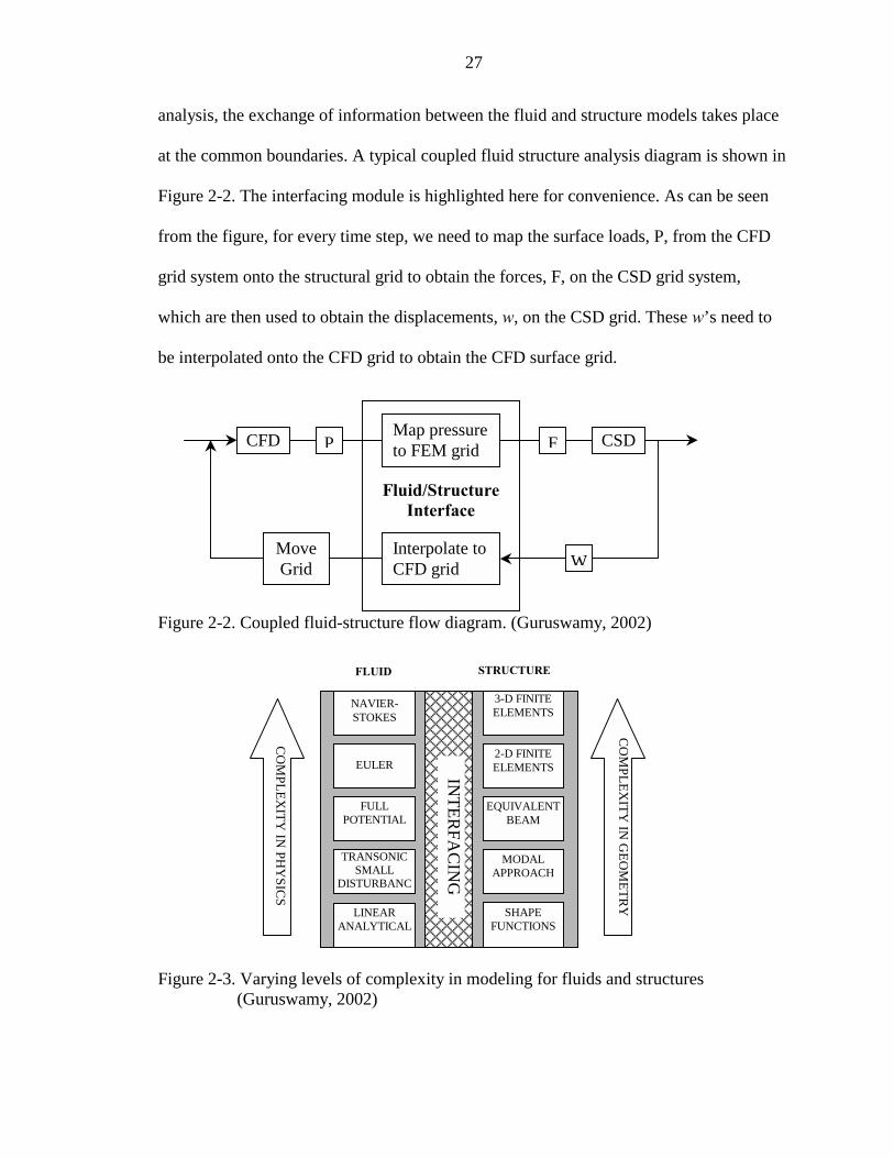
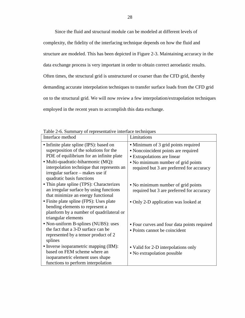
27
analysis, the exchange of information between the fluid and structure models takes place
at the common boundaries. A typical coupled fluid structure analysis diagram is shown in
Figure 2-2. The interfacing module is highlighted here for convenience. As can be seen
from the figure, for every time step, we need to map the surface loads, P, from the CFD
grid system onto the structural grid to obtain the forces, F, on the CSD grid system,
which are then used to obtain the displacements, w, on the CSD grid. These w’s need to
be interpolated onto the CFD grid to obtain the CFD surface grid.
Figure 2-2. Coupled fluid-structure flow diagram. (Guruswamy, 2002)
Figure 2-3. Varying levels of complexity in modeling for fluids and structures
(Guruswamy, 2002)
CFD P FMap pressure to FEM grid
Interpolate to CFD grid
CSD
Move Grid
Fluid/Structure Interface
W
NAVIER-STOKES
LINEAR ANALYTICAL
EULER
FULL POTENTIAL
TRANSONIC SMALL
DISTURBANCE
SHAPE FUNCTIONS
MODAL APPROACH
3-D FINITE ELEMENTS
2-D FINITE ELEMENTS
EQUIVALENT BEAM
FLUID STRUCTURE
INTER
FAC
ING
CO
MPLEX
ITY IN
PHY
SICS
CO
MPLEX
ITY IN
GEO
METR
Y
28
Since the fluid and structural module can be modeled at different levels of
complexity, the fidelity of the interfacing technique depends on how the fluid and
structure are modeled. This has been depicted in Figure 2-3. Maintaining accuracy in the
data exchange process is very important in order to obtain correct aeroelastic results.
Often times, the structural grid is unstructured or coarser than the CFD grid, thereby
demanding accurate interpolation techniques to transfer surface loads from the CFD grid
on to the structural grid. We will now review a few interpolation/extrapolation techniques
employed in the recent years to accomplish this data exchange.
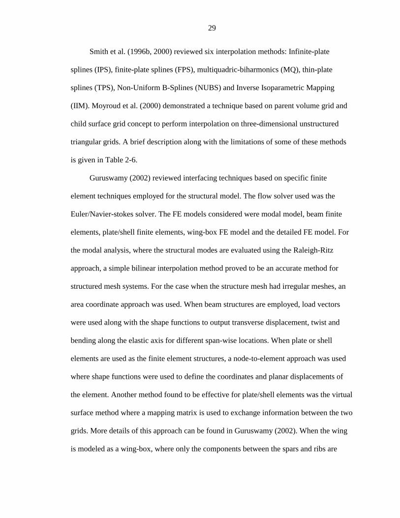
Table 2-6. Summary of representative interface techniques Interface method Limitations • Infinite plate spline (IPS): based on
superposition of the solutions for the PDE of equilibrium for an infinite plate
• Multi-quadratic-biharmonic (MQ): interpolation technique that represents an irregular surface – makes use if quadratic basis functions
• Thin plate spline (TPS): Characterizes an irregular surface by using functions that minimize an energy functional
• Finite plate spline (FPS): Uses plate bending elements to represent a planform by a number of quadrilateral or triangular elements
• Non-uniform B-splines (NUBS): uses the fact that a 3-D surface can be represented by a tensor product of 2 splines
• Inverse isoparametric mapping (IIM): based on FEM scheme where an isoparametric element uses shape functions to perform interpolation
• Minimum of 3 grid points required • Noncoincident points are required • Extrapolations are linear • No minimum number of grid points
required but 3 are preferred for accuracy • No minimum number of grid points
required but 3 are preferred for accuracy • Only 2-D application was looked at • Four curves and four data points required • Points cannot be coincident • Valid for 2-D interpolations only • No extrapolation possible
29
Smith et al. (1996b, 2000) reviewed six interpolation methods: Infinite-plate
splines (IPS), finite-plate splines (FPS), multiquadric-biharmonics (MQ), thin-plate
splines (TPS), Non-Uniform B-Splines (NUBS) and Inverse Isoparametric Mapping
(IIM). Moyroud et al. (2000) demonstrated a technique based on parent volume grid and
child surface grid concept to perform interpolation on three-dimensional unstructured
triangular grids. A brief description along with the limitations of some of these methods
is given in Table 2-6.
Guruswamy (2002) reviewed interfacing techniques based on specific finite
element techniques employed for the structural model. The flow solver used was the
Euler/Navier-stokes solver. The FE models considered were modal model, beam finite
elements, plate/shell finite elements, wing-box FE model and the detailed FE model. For
the modal analysis, where the structural modes are evaluated using the Raleigh-Ritz
approach, a simple bilinear interpolation method proved to be an accurate method for
structured mesh systems. For the case when the structure mesh had irregular meshes, an
area coordinate approach was used. When beam structures are employed, load vectors
were used along with the shape functions to output transverse displacement, twist and
bending along the elastic axis for different span-wise locations. When plate or shell
elements are used as the finite element structures, a node-to-element approach was used
where shape functions were used to define the coordinates and planar displacements of
the element. Another method found to be effective for plate/shell elements was the virtual
surface method where a mapping matrix is used to exchange information between the two
grids. More details of this approach can be found in Guruswamy (2002). When the wing
is modeled as a wing-box, where only the components between the spars and ribs are
30
considered for modeling purposes, a discrepancy might occur as there is a discontinuity
in surface at the leading and trailing edges. In such cases, forces are lumped onto
structural nodes and bending and twisting moment conservation is enforced. Deflection at
the FEM nodes were obtained by using transformation functions by assuming that the
wing is chordwise rigid. Brown (1997) proposed a method that combines the node-to-
element approach used for plate/shell FE and the lumped method for wing-box structures.
For detailed FE models, where the interior of the FE grid could be irregular and the
surface elements could take both triangular and quadrilateral elements, the area
coordinate method of the virtual surface method was found to be an efficient one.
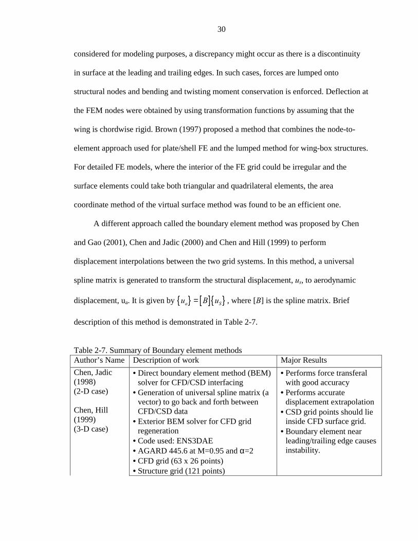
A different approach called the boundary element method was proposed by Chen
and Gao (2001), Chen and Jadic (2000) and Chen and Hill (1999) to perform
displacement interpolations between the two grid systems. In this method, a universal
spline matrix is generated to transform the structural displacement, us, to aerodynamic
displacement, ua. It is given by [ ] a Su B u= , where [B] is the spline matrix. Brief
description of this method is demonstrated in Table 2-7.
Table 2-7. Summary of Boundary element methods Author’s Name Description of work Major Results Chen, Jadic (1998) (2-D case) Chen, Hill (1999) (3-D case)
• Direct boundary element method (BEM) solver for CFD/CSD interfacing
• Generation of universal spline matrix (a vector) to go back and forth between CFD/CSD data
• Exterior BEM solver for CFD grid regeneration
• Code used: ENS3DAE • AGARD 445.6 at M=0.95 and α=2 • CFD grid (63 x 26 points) • Structure grid (121 points)
• Performs force transferal with good accuracy
• Performs accurate displacement extrapolation
• CSD grid points should lie inside CFD surface grid.
• Boundary element near leading/trailing edge causes instability.
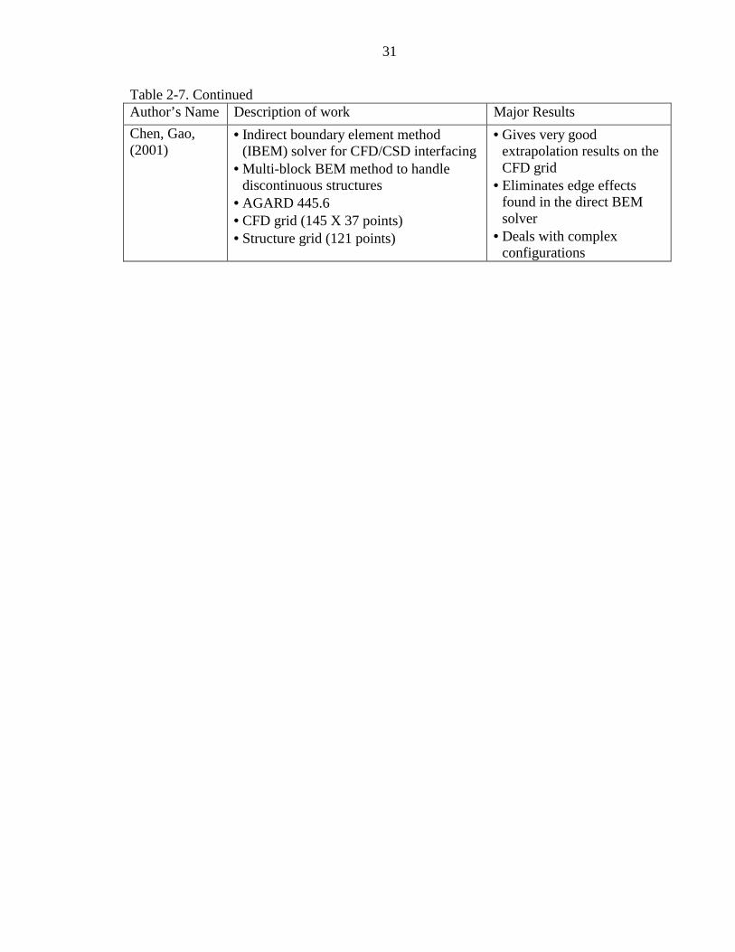
31
Table 2-7. Continued Author’s Name Description of work Major Results Chen, Gao, (2001)
• Indirect boundary element method (IBEM) solver for CFD/CSD interfacing
• Multi-block BEM method to handle discontinuous structures
• AGARD 445.6 • CFD grid (145 X 37 points) • Structure grid (121 points)
• Gives very good extrapolation results on the CFD grid
• Eliminates edge effects found in the direct BEM solver
• Deals with complex configurations
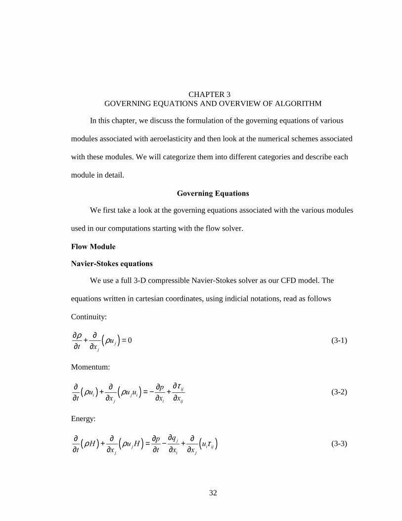
32
CHAPTER 3 GOVERNING EQUATIONS AND OVERVIEW OF ALGORITHM
In this chapter, we discuss the formulation of the governing equations of various
modules associated with aeroelasticity and then look at the numerical schemes associated
with these modules. We will categorize them into different categories and describe each
module in detail.
Governing Equations
We first take a look at the governing equations associated with the various modules
used in our computations starting with the flow solver.
Flow Module
Navier-Stokes equations
We use a full 3-D compressible Navier-Stokes solver as our CFD model. The
equations written in cartesian coordinates, using indicial notations, read as follows
Continuity:
( ) 0jj
ut xρ ρ∂ ∂+ =
∂ ∂ (3-1)
Momentum:
( ) ( ) iji j i
j i ij
pu u ut x x x
τρ ρ
∂∂ ∂ ∂+ = − +∂ ∂ ∂ ∂
(3-2)
Energy:
( ) ( ) ( )jj i ij
j i j
qpH u H ut x t x x
ρ ρ τ∂∂ ∂ ∂ ∂+ = − +
∂ ∂ ∂ ∂ ∂ (3-3)
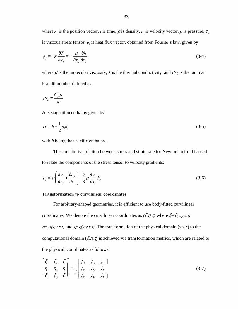
33
where xi is the position vector, t is time, ρ is density, ui is velocity vector, p is pressure, τij
is viscous stress tensor, qj is heat flux vector, obtained from Fourier’s law, given by
jj L j
T hqx Pr x
µκ ∂ ∂= − = −∂ ∂
(3-4)
where µ is the molecular viscosity, κ is the thermal conductivity, and PrL is the laminar
Prandtl number defined as:
pL
CPr
µκ
=
H is stagnation enthalpy given by
12 i iH h u u= + (3-5)
with h being the specific enthalpy.
The constitutive relation between stress and strain rate for Newtonian fluid is used
to relate the components of the stress tensor to velocity gradients:
23
ji lij ij
j i l
uu ux x x
τ µ µ δ ∂∂ ∂= + − ∂ ∂ ∂
(3-6)
Transformation to curvilinear coordinates
For arbitrary-shaped geometries, it is efficient to use body-fitted curvilinear
coordinates. We denote the curvilinear coordinates as (ξ,η,ς) where ξ=ξ(x,y,z,t),
η=η(x,y,z,t) and ς=ς(x,y,z,t). The transformation of the physical domain (x,y,z) to the
computational domain (ξ,η,ς) is achieved via transformation metrics, which are related to
the physical, coordinates as follows.
11 12 13
21 22 23
31 32 33
1x y z
x y z
x y z
f f ff f f
Jf f f
ξ ξ ξη η ηζ ζ ζ
=
(3-7)
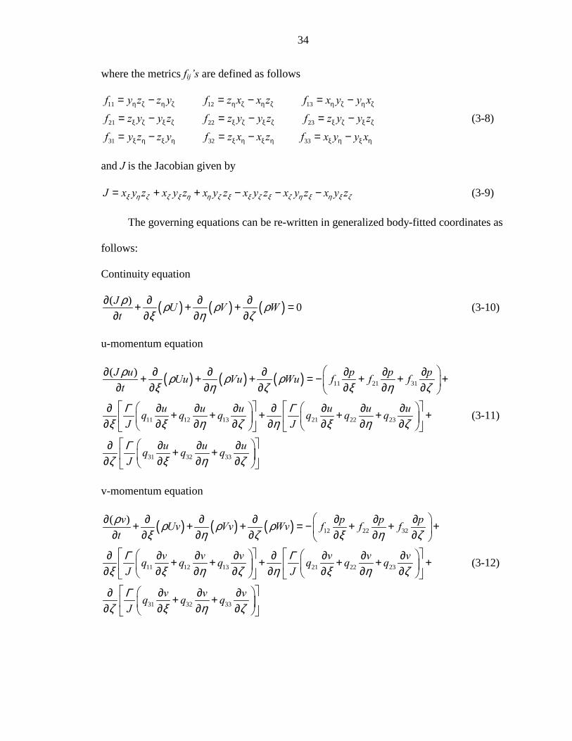
34
where the metrics fijs are defined as follows
11 12 13
21 22 23
31 32 33
f y z z y f z x x z f x y y xf z y y z f z y y z f z y y zf y z z y f z x x z f x y y x
η ζ η ζ η ζ η ζ η ζ η ζ
ξ ζ ξ ζ ξ ζ ξ ζ ξ ζ ξ ζ
ξ η ξ η ξ η ξ η ξ η ξ η
= − = − = −= − = − = −
= − = − = −
(3-8)
and J is the Jacobian given by
J x y z x y z x y z x y z x y z x y zξ η ζ ζ ξ η η ζ ξ ξ ζ ξ ζ η ξ η ξ ζ= + + − − − (3-9)
The governing equations can be re-written in generalized body-fitted coordinates as
follows:
Continuity equation
( ) ( ) ( )( ) 0J U V Wtρ ρ ρ ρ
ξ η ζ∂ ∂ ∂ ∂+ + + =
∂ ∂ ∂ ∂ (3-10)
u-momentum equation
( ) ( ) ( ) 11 21 31
11 12 13 21 22 23
31 32 33
( )J u p p pUu Vu Wu f f ft
u u u u u uq q q q q qJ J
u u uq q qJ
ρ ρ ρ ρξ η ζ ξ η ζ
Γ Γξ ξ η ζ η ξ η ζ
Γζ ξ η ζ
∂ ∂ ∂ ∂ ∂ ∂ ∂+ + + = − + + + ∂ ∂ ∂ ∂ ∂ ∂ ∂ ∂ ∂ ∂ ∂ ∂ ∂ ∂ ∂+ + + + + + ∂ ∂ ∂ ∂ ∂ ∂ ∂ ∂ ∂ ∂ ∂ ∂+ + ∂ ∂ ∂ ∂
(3-11)
v-momentum equation
( ) ( ) ( ) 12 22 32
11 12 13 21 22 23
31 32 33
( )v p p pUv Vv Wv f f ft
v v v v v vq q q q q qJ J
v v vq q qJ
ρ ρ ρ ρξ η ζ ξ η ζ
Γ Γξ ξ η ζ η ξ η ζ
Γζ ξ η ζ
∂ ∂ ∂ ∂ ∂ ∂ ∂+ + + = − + + + ∂ ∂ ∂ ∂ ∂ ∂ ∂ ∂ ∂ ∂ ∂ ∂ ∂ ∂ ∂+ + + + + + ∂ ∂ ∂ ∂ ∂ ∂ ∂ ∂ ∂ ∂ ∂ ∂+ + ∂ ∂ ∂ ∂
(3-12)
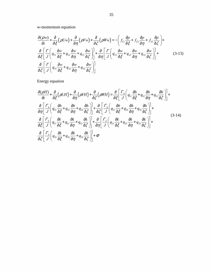
35
w-momentum equation
( ) ( ) ( ) 13 23 33
11 12 13 21 22 23
31 32 33
( )w p p pUw Vw Ww f f ft
w w w w w wq q q q q qJ J
w w wq q qJ
ρ ρ ρ ρξ η ζ ξ η ζ
Γ Γξ ξ η ζ η ξ η ζ
Γζ ξ η ζ
∂ ∂ ∂ ∂ ∂ ∂ ∂+ + + = − + + + ∂ ∂ ∂ ∂ ∂ ∂ ∂ ∂ ∂ ∂ ∂ ∂ ∂ ∂ ∂+ + + + + + ∂ ∂ ∂ ∂ ∂ ∂ ∂ ∂ ∂ ∂ ∂ ∂+ + ∂ ∂ ∂ ∂
(3-13)
Energy equation
( ) ( ) ( ) 11 12 13
21 22 23 31 32 33
11 12 13
( ) h
h h
k
H h h hUH VH WH q q qt J
h h h h h hq q q q q qJ J
k k kq q qJ
Γρ ρ ρ ρξ η ζ ξ ξ η ζ
Γ Γη ξ η ζ ζ ξ η ζ
Γξ ξ η ζ η
∂ ∂ ∂ ∂ ∂ ∂ ∂ ∂+ + + = + + + ∂ ∂ ∂ ∂ ∂ ∂ ∂ ∂ ∂ ∂ ∂ ∂ ∂ ∂ ∂ ∂+ + + + + + ∂ ∂ ∂ ∂ ∂ ∂ ∂ ∂ ∂ ∂ ∂ ∂ ∂+ + + ∂ ∂ ∂ ∂ ∂
21 22 23
31 32 33
k
k
k k kq q qJ
k k kq q qJ
Γξ η ζ
Γ Φζ ξ η ζ
∂ ∂ ∂+ + + ∂ ∂ ∂ ∂ ∂ ∂ ∂+ + + ∂ ∂ ∂ ∂
(3-14)
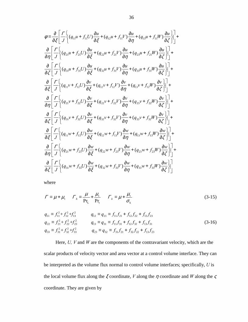
36
11 11 12 11 13 11
21 21 22 21 23 21
31 31 32 31 33 31
( ) ( ) ( )
( ) ( ) ( )
( ) ( ) ( )
u u uq u f U q u f V q u f WJ
u u uq u f U q u f V q u f WJ
u u uq u f U q u f V q u f WJ
Γφξ ξ η ζ
Γη ξ η ζ
Γζ ξ η ζ
ξ
∂ ∂ ∂ ∂= + + + + + + ∂ ∂ ∂ ∂ ∂ ∂ ∂ ∂+ + + + + + ∂ ∂ ∂ ∂ ∂ ∂ ∂ ∂+ + + + + + ∂ ∂ ∂ ∂
∂∂ 11 12 12 12 13 12
21 22 22 22 23 22
31 32 32 32 33 32
1
( ) ( ) ( )
( ) ( ) ( )
( ) ( ) ( )
(
v v vq v f U q v f V q v f WJ
v v vq v f U q v f V q v f WJ
v v vq v f U q v f V q v f WJ
qJ
Γξ η ζ
Γη ξ η ζ
Γζ ξ η ζ
Γξ
∂ ∂ ∂+ + + + + + ∂ ∂ ∂ ∂ ∂ ∂ ∂+ + + + + + ∂ ∂ ∂ ∂ ∂ ∂ ∂ ∂+ + + + + + ∂ ∂ ∂ ∂
∂∂ 1 13 12 13 13 13
21 23 22 23 23 23
31 33 32 33 33 33
) ( ) ( )
( ) ( ) ( )
( ) ( ) ( )
w w ww f U q w f V q w f W
w w wq w f U q w f V q w f WJ
w w wq w f U q w f V q w f WJ
ξ η ζ
Γη ξ η ζ
Γζ ξ η ζ
∂ ∂ ∂+ + + + + + ∂ ∂ ∂ ∂ ∂ ∂ ∂+ + + + + + ∂ ∂ ∂ ∂ ∂ ∂ ∂ ∂+ + + + + ∂ ∂ ∂ ∂
where
t tt
L t kPr Prh k µ µµΓ µ µ Γ Γ µσ
= + = + = + (3-15)
2 2 211 11 12 13 12 21 11 21 12 22 13 23
2 2 222 21 22 23 13 31 11 31 12 32 13 31
2 2 233 31 32 33 23 32 31 21 32 22 13 23
+ +
+ + + +
q f f f q q f f f f f fq f f f q q f f f f f fq f f f q q f f f f f f
= = = + +
= = = + +
= = = + +
(3-16)
Here, U, V and W are the components of the contravariant velocity, which are the
scalar products of velocity vector and area vector at a control volume interface. They can
be interpreted as the volume flux normal to control volume interfaces; specifically, U is
the local volume flux along the ξ coordinate, V along the η coordinate and W along the ς
coordinate. They are given by
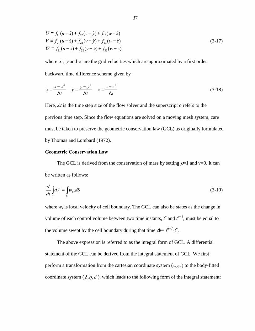
37
11 12 13
21 22 23
31 32 33
( ) ( ) ( )( ) ( ) ( )( ) ( ) ( )
U f u x f v y f w zV f u x f v y f w zW f u x f v y f w z
= − + − + −= − + − + −= − + − + −
! ! !! ! !! ! !
(3-17)
where x! , y! and z! are the grid velocities which are approximated by a first order
backward time difference scheme given by
o o ox x y y z zx y z
t t t− − −= = =∆ ∆ ∆
! ! ! (3-18)
Here, ∆t is the time step size of the flow solver and the superscript o refers to the
previous time step. Since the flow equations are solved on a moving mesh system, care
must be taken to preserve the geometric conservation law (GCL) as originally formulated
by Thomas and Lombard (1972).
Geometric Conservation Law
The GCL is derived from the conservation of mass by setting ρ=1 and v=0. It can
be written as follows:
.V S
d dV dSdt
=∫ ∫ sw (3-19)
where ws is local velocity of cell boundary. The GCL can also be states as the change in
volume of each control volume between two time instants, tn and tn+1, must be equal to
the volume swept by the cell boundary during that time ∆t= tn+1-tn.
The above expression is referred to as the integral form of GCL. A differential
statement of the GCL can be derived from the integral statement of GCL. We first
perform a transformation from the cartesian coordinate system (x,y,z) to the body-fitted
coordinate system ( , ,ξ η ζ ), which leads to the following form of the integral statement:

38
( )ξ η ζ = ∇ ξ η ζ∫ ∫V V
d Jd d d Jd d ddt s.w (3-20)
Here, J represents the volume element in the transformed coordinate system hence
each node is associated with a particular value of J. Therefore, the computed value of J
must be consistent with the value of ∆V implied by the numerical scheme used for
solving the flow equations. Earlier, arbitrary procedures were used to compute J, for e.g.,
instantaneous mesh distribution at a given time instant was used to evaluate J at that
particular time, which lead to an erroneous solution.
Expanding the right hand side of Eq. (3-20) and after performing necessary
manipulations, we arrive at the following form for the differential statement of GCL.
( ) ( ) ( ) 0t t t tJ ξ η ζξ η ζ+ + + = (3-21)
where, , ,t t tξ η ζ are the metric terms given by
( )( )( )
( ) ( )
( ) ( )
( ) ( )
t
t
t
x y z y z y z x z x z x y x y
x y z y z y z x z x z x y x y
x y z y z y z x z x z x y x y
η ζ ζ η η ζ ζ η η ζ ζ η
ζ ξ ξ ζ ζ ξ ξ ζ ζ ξ ξ ζ
ξ η η ξ ξ η η ξ ξ η η ξ
ξ
η
ζ
= − − + − + − = − − + − + − = − − + − + −
! ! !
! ! !
! ! !
(3-22)
Equation (3-21) is solved numerically to update the Jacobian values at each time
step. The numerical solution for Eq. (3-21) requires only an initial condition, which is
obtained from the initial fixed grid and is given by Eq. (3-9).
Turbulence Modeling
The conservation equations (3-1) - (3-3) hold good only for laminar flows. For
turbulent flows, we need to re-construct the equations based on an averaging process in
the context of RANS methods.
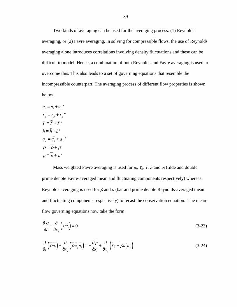
39
Two kinds of averaging can be used for the averaging process: (1) Reynolds
averaging, or (2) Favre averaging. In solving for compressible flows, the use of Reynolds
averaging alone introduces correlations involving density fluctuations and these can be
difficult to model. Hence, a combination of both Reynolds and Favre averaging is used to
overcome this. This also leads to a set of governing equations that resemble the
incompressible counterpart. The averaging process of different flow properties is shown
below.
"
"
"
#
"
''
''
''
''
''
'
'
i i i
ij ij ij
j j j
u u u
T T T
h h h
q q q
p p p
τ τ τ
ρ ρ ρ
= +
= +
= +
= +
= +
= +
= +
Mass weighted Favre averaging is used for ui, τij, T, h and qj (tilde and double
prime denote Favre-averaged mean and fluctuating components respectively) whereas
Reynolds averaging is used for ρ and p (bar and prime denote Reynolds-averaged mean
and fluctuating components respectively) to recast the conservation equation. The mean-
flow governing equations now take the form:
"( ) 0ij
ut xρ ρ∂ ∂+ =
∂ ∂ (3-23)
"( ) ""( ) ( )'' ''j j
iji j ij i j
pu u u u ut x x x
ρ ρ τ ρ∂ ∂ ∂ ∂+ = − + −∂ ∂ ∂ ∂
# (3-24)
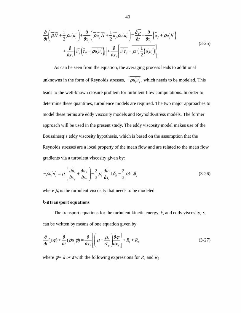
40
" "" " #( )" ( ) ( )
'' '' '' '' '' ''
'' '' '' '' '' ''
1 12 2
1 2
i i j j i i jjj j
ijj i j i ij j i ij j
pH u u u H u u u q u ht x t x
u u u u u u ux x
ρ ρ ρ ρ ρ
τ ρ τ ρ
∂ ∂ ∂ ∂ + + + = − + ∂ ∂ ∂ ∂
∂ ∂ + − + − ∂ ∂ #
(3-25)
As can be seen from the equation, the averaging process leads to additional
unknowns in the form of Reynolds stresses, '' ''i ju uρ− , which needs to be modeled. This
leads to the well-known closure problem for turbulent flow computations. In order to
determine these quantities, turbulence models are required. The two major approaches to
model these terms are eddy viscosity models and Reynolds-stress models. The former
approach will be used in the present study. The eddy viscosity model makes use of the
Boussinesq’s eddy viscosity hypothesis, which is based on the assumption that the
Reynolds stresses are a local property of the mean flow and are related to the mean flow
gradients via a turbulent viscosity given by:
# # #'' '' 2 2
3 3i j l
i j t t ij ijj i l
u u uu u kx x x
ρ µ µ δ ρ δ ∂ ∂ ∂− = + − ⋅ − ⋅ ∂ ∂ ∂
(3-26)
where µt is the turbulent viscosity that needs to be modeled.
k-εεεε transport equations
The transport equations for the turbulent kinetic energy, k, and eddy viscosity, ε,
can be written by means of one equation given by:
1 2( ) ( ) tj
j j
u R Rt t x xφ
µ φρφ ρ φ µσ
∂ ∂ ∂ ∂+ = + + + ∂ ∂ ∂ ∂ (3-27)
where φ = k or ε with the following expressions for R1 and R2
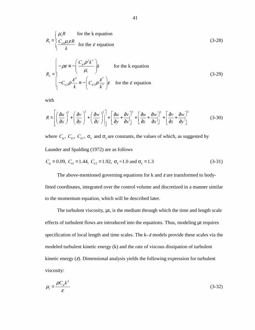
41
1 1
for the k equation
for the equation
t
t
RR C R
kε
µµ ε ε
=
(3-28)
2 *
22 *
2 2 *
for the k equation
for the equation
t
C kk
R
C Ck k
µ
ε ε
ρρε
µ
ε ερ ρ ε ε
− ≡ − =
− ≡ −
(3-29)
with
2 2 22 2 2u v w u v u w v wRx y z y x z x z y
∂ ∂ ∂ ∂ ∂ ∂ ∂ ∂ ∂ = + + + + + + + + ∂ ∂ ∂ ∂ ∂ ∂ ∂ ∂ ∂ (3-30)
where 1 2, , , and kC C Cµ ε ε εσ σ are constants, the values of which, as suggested by
Launder and Spalding (1972) are as follows
1 20.09, 1.44, 1.92, =1.0 and 1.3kC C Cµ ε ε ε= = = σ σ = (3-31)
The above-mentioned governing equations for k and ε are transformed to body-
fitted coordinates, integrated over the control volume and discretized in a manner similar
to the momentum equation, which will be described later.
The turbulent viscosity, µt, is the medium through which the time and length scale
effects of turbulent flows are introduced into the equations. Thus, modeling µt requires
specification of local length and time scales. The k–ε models provide these scales via the
modeled turbulent kinetic energy (k) and the rate of viscous dissipation of turbulent
kinetic energy (ε). Dimensional analysis yields the following expression for turbulent
viscosity:
2
t
C kµρµ
ε= (3-32)
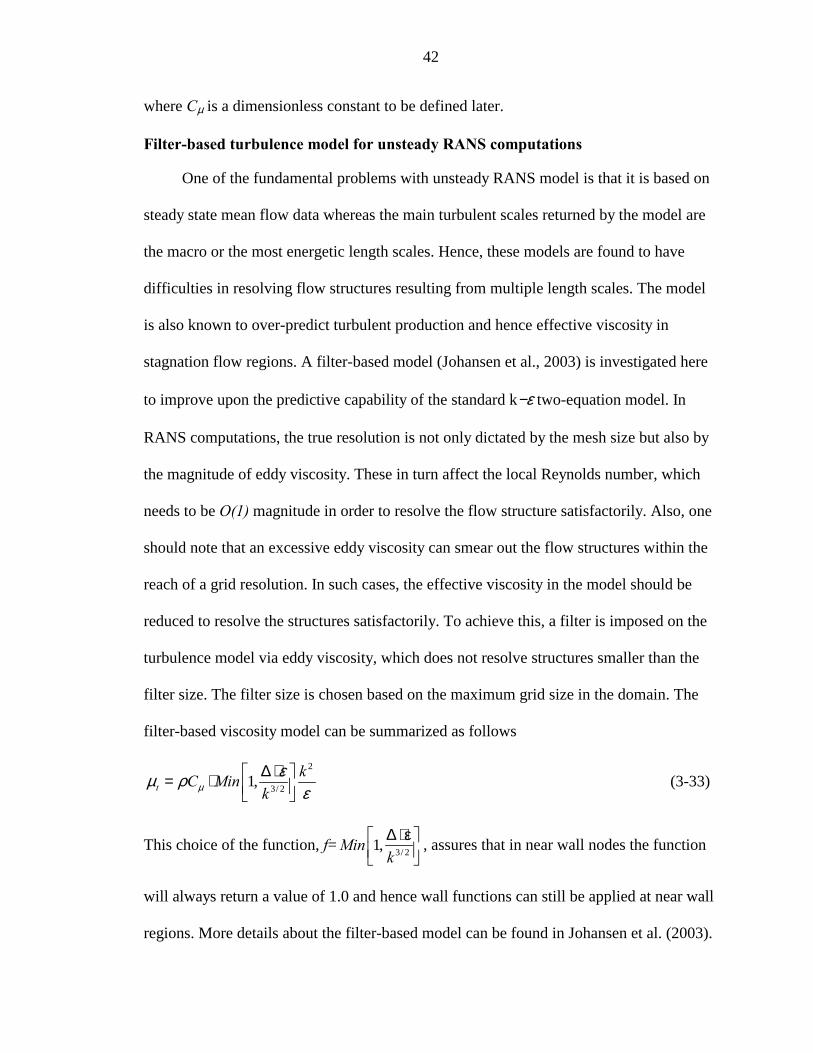
42
where Cµ is a dimensionless constant to be defined later.
Filter-based turbulence model for unsteady RANS computations
One of the fundamental problems with unsteady RANS model is that it is based on
steady state mean flow data whereas the main turbulent scales returned by the model are
the macro or the most energetic length scales. Hence, these models are found to have
difficulties in resolving flow structures resulting from multiple length scales. The model
is also known to over-predict turbulent production and hence effective viscosity in
stagnation flow regions. A filter-based model (Johansen et al., 2003) is investigated here
to improve upon the predictive capability of the standard k−ε two-equation model. In
RANS computations, the true resolution is not only dictated by the mesh size but also by
the magnitude of eddy viscosity. These in turn affect the local Reynolds number, which
needs to be O(1) magnitude in order to resolve the flow structure satisfactorily. Also, one
should note that an excessive eddy viscosity can smear out the flow structures within the
reach of a grid resolution. In such cases, the effective viscosity in the model should be
reduced to resolve the structures satisfactorily. To achieve this, a filter is imposed on the
turbulence model via eddy viscosity, which does not resolve structures smaller than the
filter size. The filter size is chosen based on the maximum grid size in the domain. The
filter-based viscosity model can be summarized as follows
2
3/ 21,tkC Min
kµεµ ρ
ε∆ ⋅ = ⋅
(3-33)
This choice of the function, f= 3/ 21,Mink∆ ⋅ε
, assures that in near wall nodes the function
will always return a value of 1.0 and hence wall functions can still be applied at near wall
regions. More details about the filter-based model can be found in Johansen et al. (2003).
43
Boundary conditions
Boundary condition needs to be specified due to the elliptic nature of the k-ε
equations. All the variables at the inlet are either specified or estimated. If the inlet
velocity is specified, k is estimated based on a fraction of the square of the inlet velocity
and ε is estimated from k and a characteristic length scale representing the size of the
turbulent eddies (usually a fraction of the inlet dimension). The estimates for k and ε are
given by
( )232 ik U T∞= (3-34)
3/ 4 3/ 2
0.07C k
Lµε =
where iT is the turbulence intensity usually set in the range of 0.02 and 0.05 and L is a
typical inlet dimension length scale. The outlet boundary conditions are determined via a
zero gradient condition based on the assumption that the flow is convection-dominated.
Wall treatment
Near wall boundaries, the local Reynolds number is of the order of one and hence
viscous effects are more dominant, hence the k-ε model cannot be used as it is formulated
based on the assumption of high Reynolds number. Two approaches have been proposed
to handle near-wall effects, one being the low Reynolds number model and the other
being wall-function method. The former method requires a very fine grid resolution near
the wall and hence makes the computations expensive. The latter method is based on the
assumption that there exists local equilibrium between production and dissipation of
turbulent kinetic energy. It was proved to be an accurate and robust approximation and it
does not require a fine grid near the wall or boundary.
44
For a fully developed turbulent flow near a no–slip wall, the normalized near–wall
tangential velocity, assuming a two–layer structure (viscous sublayer followed by log
layer), can be written as follows
+
+
for laminar sublayer (y 11.63)1 ln( ) for law of the wall layer (y 11.63)
yu
Ey
+
++
<=
>κ (3-35)
where κ is the von Karmen constant which has a value of 0.42 and E is a factor that
depends on wall roughness, streamwise pressure gradient, etc. It is assigned a value of
9.793 for a smooth wall. Here, +y is the local Reynolds number given by
+ nu ly τρµ
= (3-36)
and u+ is the non-dimensional velocity given by
tuuu
+
τ
= (3-37)
where uτ is the friction velocity at the wall given by
walluττ
ρ= (3-38)
The expression for the shear stress at the wall, wallτ , expressed in terms of turbulent
kinetic energy, in the log layer, is given by
1/ 4 1/ 2
ln( )
t
wall
C k uEy
µρ κ
τ += (3-39)
Structural Dynamics Model
For the current structural modeling of the wing, only linear effects will be
considered (Kamakoti et al., 2002). This simplification allows for a good description of
45
the motion of the wing, without being computationally hampered by complex nonlinear
effects. Since the wing is to be modeled as a linear structure, it is possible to model the
deformations as a summation of different modes of deformation without looking at the
complex interaction of the modes. To this end, we choose to model the wing as a linear
finite element structure that can undergo bending and torsion. It is also important to note
that we choose to keep the cross sections of the wing rigid, further uncoupling the
bending and torsional displacements.
The linear finite element that we choose to model the wing is a beam that has mass,
stiffness, and damping matrices of the actual wing. Thus, the deformations become that
of a Bernoulli-Euler beam bending and torsion, the equations for which reads as
2 2
2 2
d d wEI pdx dx
=
(3-40)
where p is the distributed loading (force per unit length) acting in the same direction as
the out-of-plane displacement (w), E is the Young's modulus of the beam, and I is the
area moment of inertia of the beam's cross section. Since, the cross sections of the wing
are assumed to be rigid, there is a point at which the vertical displacement of the beam is
a result of only the bending of the wing. This point is where the elastic axis of the wing
intersects the cross section. The generalized displacements from bending and torsion are
measured from this point. This has been depicted in Figure 3-1.
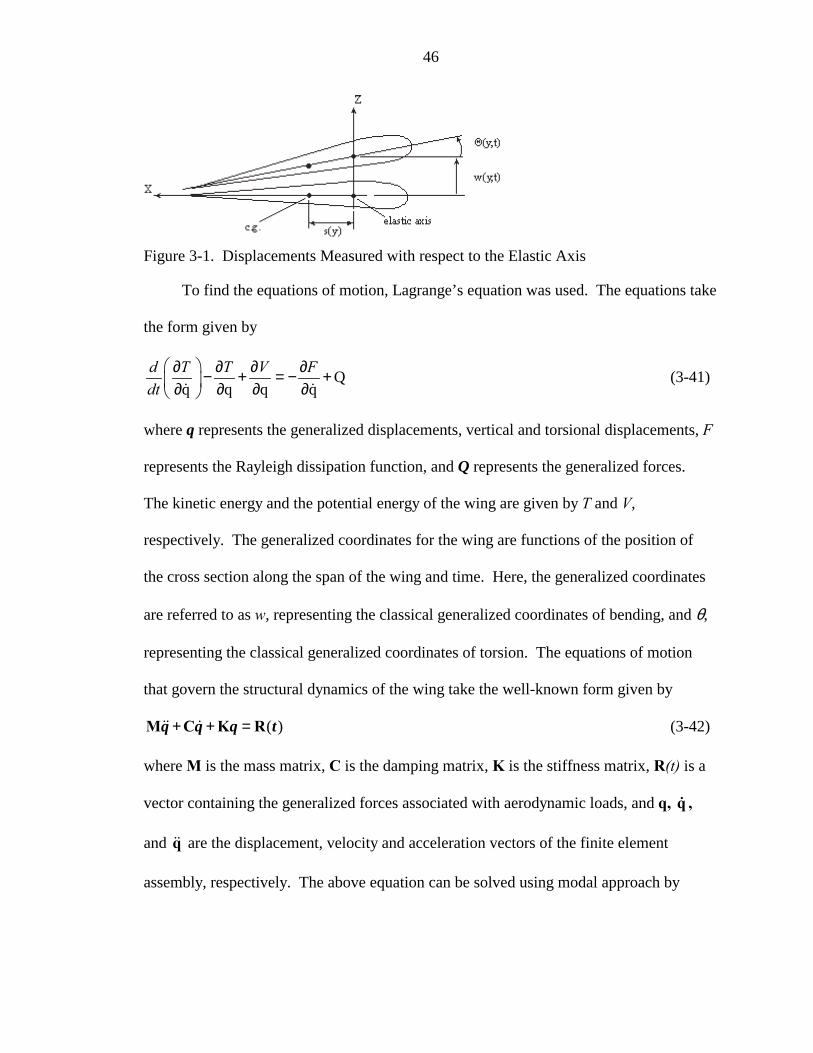
46
Figure 3-1. Displacements Measured with respect to the Elastic Axis
To find the equations of motion, Lagrange’s equation was used. The equations take
the form given by
Qq q q q
d T T V Fdt ∂ ∂ ∂ ∂− + = − + ∂ ∂ ∂ ∂ ! !
(3-41)
where q represents the generalized displacements, vertical and torsional displacements, F
represents the Rayleigh dissipation function, and Q represents the generalized forces.
The kinetic energy and the potential energy of the wing are given by T and V,
respectively. The generalized coordinates for the wing are functions of the position of
the cross section along the span of the wing and time. Here, the generalized coordinates
are referred to as w, representing the classical generalized coordinates of bending, and θ,
representing the classical generalized coordinates of torsion. The equations of motion
that govern the structural dynamics of the wing take the well-known form given by
( )+ + =M C K R!! !q q q t (3-42)
where M is the mass matrix, C is the damping matrix, K is the stiffness matrix, R(t) is a
vector containing the generalized forces associated with aerodynamic loads, and q, q!!!! ,
and q!! are the displacement, velocity and acceleration vectors of the finite element
assembly, respectively. The above equation can be solved using modal approach by
47
composing the solution with the eigenvectors of the vibration problem, i.e., the
displacement vector can be written as
; ;= = =q Z q Z q Z! !!! !!Φ Φ ΦΦ Φ ΦΦ Φ ΦΦ Φ Φ (3-43)
where ΦΦΦΦ is the modal matrix containing the eigenvectors, orthonormalized with the mass
matrix, and Z is the generalized displacement. The eigenvectors are orthogonal to both
mass and stiffness matrices and if we assume Rayleigh damping, it is also orthogonal to
the damping matrix. Pre-multiplying Eq. (3-42) by ΦΦΦΦΤ, we get
t + t + t = t2T TZ( ) Φ CΦZ( ) Ω Z( ) Φ R( )!! ! (3-44)
where
2 , 1Φ Φ = Φ Φ =T TK Ω M (3-45)
The initial conditions on Z(t) are obtained using Eq. (3-43) at time 0, as follows
0
0
0
0
=
=
Φ
Φ
T
T
Mq
Mq
ZZ !!
Equation (3-44) can be written as n individual equations, one for each mode, as follows
2( ) ( ) ( ) ( )
( ) ( )
2Ti
i i i i i i i
i
z t t t t i = 1, 2, . . . , n
t tz z r
rξ ω ω
= Φ
+ + =R
!! !! (3-46)
with initial conditions
0
0
|
|
Ti t=0 i
Ti t=0 i
xx
=
=
ΦΦ
Mq
Mq!!
Here ωi is the natural frequency for the ith mode and ξi is the corresponding damping
parameter for that mode. The solution to the above equation can be obtained for each
mode using direct integration algorithms. The structural solver integrates these equations
of motion in time for one time step given the time step size, the pressures on structural
48
nodes at the initial time, and the initial geometry of the wing. It uses an implicit
Newmark scheme for temporal calculations and hence is not limited by a time step size
unlike other explicit methods.
Moving Grid Module
For fluid/structure interaction problems, we must account for grid movement along
the deformed surface. Since the structure moves after every time step, we need to
accommodate this movement in the CFD domain. This is usually done with some type of
dynamics related mesh algorithm. In our approach, we use the perturbation method for
single block grid, which is a TFI-like method as proposed by Eriksson (1982). A main
feature of the perturbation method is that it regenerates the computational grid based on
the original grid, hence it has the capability to preserve the quality of the original grid.
For a one-dimensional problem, it uses a simple formula based on spring analogy,
originally proposed by Batina (1989) for tetrahedral cells and later extended by Robison
et al. (1991) for hexahedral cells, given by
( )new old old new oldi i i s sx x S x x= + − (3-47)
where xi represents the location of interior grid point, xs the location of grid point on a
boundary, and S the normalized arc length along the radial mesh line measured from the
outer domain. Specifically,
2 2 21 1 1 1
2 2 21 1 1 1
( ) ( ) ( )
( ) ( ) ( )
il l l l l l l
i nl l l l l l l
x x y y z zS
x x y y z z= + + +
= + + +
Σ − + − + −=
Σ − + − + − (3-48)
To use this one-dimensional perturbation method, we only need to know the
displacements of the end points. The positions of the interim points are solely determined
based on the displacements of these end points. Here, we consider such displacements as
49
the source of perturbation. By design, a perturbation will spread throughout the whole
domain, but exerts more effect on points near the boundary perturbed. Based on Eq.
(3-47), a more general 3-stage perturbation method is proposed for three-dimensional
problems treated by the single-block approach.
As far as the multi-block grid movement is concerned, we use the master/slave
strategy to establish a relationship between the moving surface points (master points) and
vertices located at the other blocks (slave points). The movement of the master points is
based on the displacements obtained from the structure solver. The movement of the
slave points follows its master point. A slave point, which has the coordinate of xs, moves
when its master point moves from mx# to xm. A simple but effective formula suggested by
Hartwich and Agrawal (1997), based on spring analogy, is expressed as follows:
s s m mx =x +θ(x -x )# # (3-49)
where the subscripts m and s represent master and slave, respectively, and tilde (~)
indicates the new position. θ is the decay function; here, we use the Gaussian distribution
function, as suggested by Hartwich and Agrawal (1997), given by
exp min[ , /( )]FACMIN dv dm= − +θ β ε (3-50)
where
2 2 2( ) ( ) ( )v m v m v mdv x x y y z z= − + − + − (3-51)
2 2 2( ) ( ) ( )m m m m m mdm x x y y z z= − + − + −# # # (3-52)
and ε is an arbitrary small number to eliminate division by zero.
In Eq. (3-50), the coefficient β affects the stiffness. A larger β causes the block to
behave more like a rigid body and a smaller value makes the body behave like a softball.
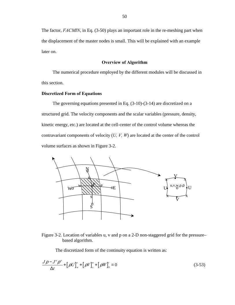
50
The factor, FACMIN, in Eq. (3-50) plays an important role in the re-meshing part when
the displacement of the master nodes is small. This will be explained with an example
later on.
Overview of Algorithm
The numerical procedure employed by the different modules will be discussed in
this section.
Discretized Form of Equations
The governing equations presented in Eq. (3-10)-(3-14) are discretized on a
structured grid. The velocity components and the scalar variables (pressure, density,
kinetic energy, etc.) are located at the cell-center of the control volume whereas the
contravariant components of velocity (U, V, W) are located at the center of the control
volume surfaces as shown in Figure 3-2.
Figure 3-2. Location of variables u, v and p on a 2-D non-staggered grid for the pressure–based algorithm.
The discretized form of the continuity equation is written as:
[ ] [ ] [ ] 0o o
e n t
w s b
J J U V Wt
ρ ρ ρ ρ ρ− + + + =∆
(3-53)
o
o
o
o oW E
N
S
Pw
s
e
n
o
x
x x
x •
•
•
•
U
V
U
V
u,v,w,p.ρ
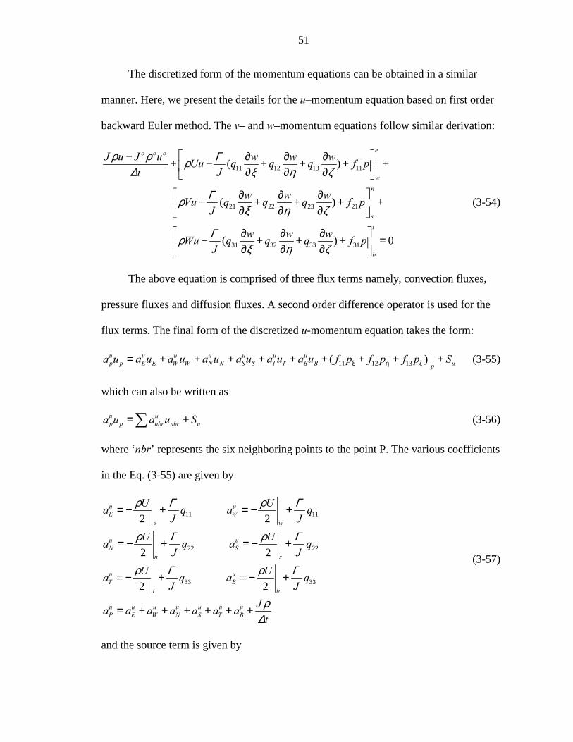
51
The discretized form of the momentum equations can be obtained in a similar
manner. Here, we present the details for the u–momentum equation based on first order
backward Euler method. The v– and w–momentum equations follow similar derivation:
11 12 13 11
21 22 23 21
31 32 33 31
( )
( )
( ) 0
eo o o
wn
st
b
J u J u w w wUu q q q f pt J
w w wVu q q q f pJ
w w wWu q q q f pJ
ρ ρ Γρ∆ ξ η ζ
Γρξ η ζ
Γρξ η ζ
− ∂ ∂ ∂+ − + + + + ∂ ∂ ∂
∂ ∂ ∂− + + + + ∂ ∂ ∂
∂ ∂ ∂− + + + = ∂ ∂ ∂
(3-54)
The above equation is comprised of three flux terms namely, convection fluxes,
pressure fluxes and diffusion fluxes. A second order difference operator is used for the
flux terms. The final form of the discretized u-momentum equation takes the form:
11 12 13( )u u u u u u up p E E W W N N S S T T B B up
a u a u a u a u a u a u a u f p f p f p Sξ η ζ= + + + + + + + + + (3-55)
which can also be written as
u up p nbr nbr ua u a u S= +∑ (3-56)
where ‘nbr’ represents the six neighboring points to the point P. The various coefficients
in the Eq. (3-55) are given by
11 11
22 22
33 33
2 2
2 2
2 2
u uE W
e w
u uN S
n s
u uT B
t b
u u u u u u uP E W N S T B
U Ua q a qJ J
U Ua q a qJ J
U Ua q a qJ J
Ja a a a a a at
ρ Γ ρ Γ
ρ Γ ρ Γ
ρ Γ ρ Γ
ρ∆
= − + = − +
= − + = − +
= − + = − +
= + + + + + +
(3-57)
and the source term is given by
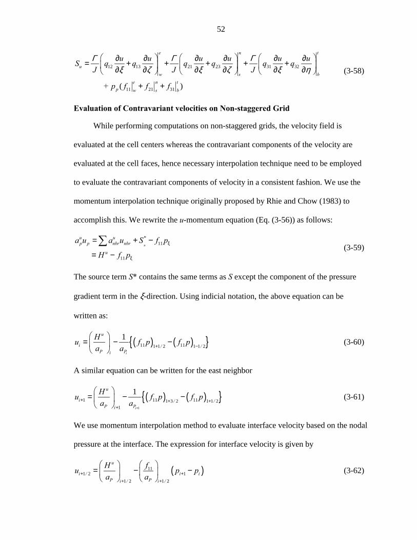
52
12 13 21 23 31 32
11 21 31( )
e n t
uw s b
e n tp w s b
u u u u u uS q q q q q qJ J J
+ p f f f
Γ Γ Γξ ζ ξ ζ ξ η
∂ ∂ ∂ ∂ ∂ ∂= + + + + + ∂ ∂ ∂ ∂ ∂ ∂
+ +
(3-58)
Evaluation of Contravariant velocities on Non-staggered Grid
While performing computations on non-staggered grids, the velocity field is
evaluated at the cell centers whereas the contravariant components of the velocity are
evaluated at the cell faces, hence necessary interpolation technique need to be employed
to evaluate the contravariant components of velocity in a consistent fashion. We use the
momentum interpolation technique originally proposed by Rhie and Chow (1983) to
accomplish this. We rewrite the u-momentum equation (Eq. (3-56)) as follows:
*11
11 u
u up p nbr nbr
u
a u a u S f p
H f pξ
ξ
= + −
= −∑
(3-59)
The source term S* contains the same terms as S except the component of the pressure
gradient term in the ξ-direction. Using indicial notation, the above equation can be
written as:
( ) ( ) 11 111 1 2 1 1 2
1
i
u
i / /P Pi
Hu f p f pa a + −
= − −
(3-60)
A similar equation can be written for the east neighbor
( ) ( ) 1
1 11 111 3 2 1 1 21
1
i
u
i / /P Pi
Hu f p f pa a
+
+ + ++
= − −
(3-61)
We use momentum interpolation method to evaluate interface velocity based on the nodal
pressure at the interface. The expression for interface velocity is given by
( )111 2 1
1 2 1 2
u
i / i iP Pi / i /
fHu p pa a+ +
+ +
= − −
(3-62)
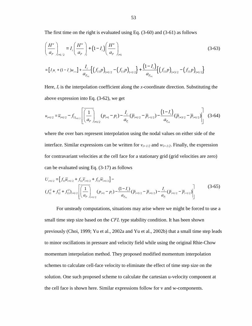
53
The first time on the right is evaluated using Eq. (3-60) and (3-61) as follows
( )1 2 1
1u u u
i iP P Pi / i i
H H HI Ia a a
+ +
= + −
(3-63)
[ ] ( ) ( ) ( ) ( ) ( ) 1
1 1
11 11 11 111 1/ 2 1 1/ 2 1 3/ 2 1 1/ 2(1 )
1i i i i
i i
ii
P P
I u I uII f p f p f p f p
a a+
+ +
+ − + += + − +
−− + −
Here, Ii is the interpolation coefficient along the x-coordinate direction. Substituting the
above expression into Eq. (3-62), we get
( )1/ 2
1
1/ 2 1/2 11 1 1/2 1/ 2 3/ 2 1/ 21/2
11 ( ) ( ) ( )i
i i
iii i i i i i i i
P P Pi
u uIIf p p p p p p
a a a+
+
+ + + + − + ++
= − − − − − − −
(3-64)
where the over bars represent interpolation using the nodal values on either side of the
interface. Similar expressions can be written for vi+1/2 and wi+1/2. Finally, the expression
for contravariant velocities at the cell face for a stationary grid (grid velocities are zero)
can be evaluated using Eq. (3-17) as follows
[ ]
1
1/ 2 11 1/ 2 12 1/ 2 13 1/ 2
2 2 211 12 13 1/ 2 1 3/ 2 1/ 2 1/ 2 1/ 2
1/ 2
(1 )1( ) ( ) ( ) ( )i i
i i i i
i ii i i i i i i
P P Pi
U f u f v f w
I If f f p p p p p pa a a
+
+ + + +
+ + + + + −+
= + + −
− + + − − − − −
(3-65)
For unsteady computations, situations may arise where we might be forced to use a
small time step size based on the CFL type stability condition. It has been shown
previously (Choi, 1999; Yu et al., 2002a and Yu et al., 2002b) that a small time step leads
to minor oscillations in pressure and velocity field while using the original Rhie-Chow
momentum interpolation method. They proposed modified momentum interpolation
schemes to calculate cell-face velocity to eliminate the effect of time step size on the
solution. One such proposed scheme to calculate the cartesian u-velocity component at
the cell face is shown here. Similar expressions follow for v and w-components.
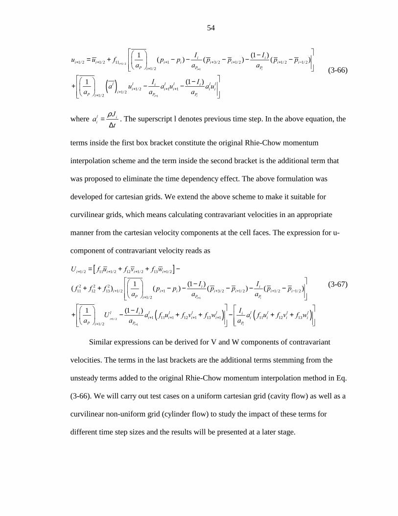
54
( )
1/ 2
1
1
1/ 2 1/ 2 11 1 3/ 2 1/ 2 1/ 2 1/ 21/ 2
1/ 2 1 11/ 2
1/ 2
(1 )1 ( ) ( ) ( )
(1 )1
i
i i
i i
i ii i i i i i i i
P P Pi
l l l l l li ii i i i i
iP P Pi
I Iu u f p p p p p pa a a
I Ia u a u a ua a a
+
+
+
+ + + + + + −+
+ + ++
+
− = + − − − − −
− + − −
(3-66)
where l ii
Jt
a ρ=
∆. The superscript l denotes previous time step. In the above equation, the
terms inside the first box bracket constitute the original Rhie-Chow momentum
interpolation scheme and the term inside the second bracket is the additional term that
was proposed to eliminate the time dependency effect. The above formulation was
developed for cartesian grids. We extend the above scheme to make it suitable for
curvilinear grids, which means calculating contravariant velocities in an appropriate
manner from the cartesian velocity components at the cell faces. The expression for u-
component of contravariant velocity reads as
[ ]
1
1/ 2
1
1/ 2 11 1/ 2 12 1/ 2 13 1/ 2
2 2 211 12 13 1/ 2 1 3/ 2 1/ 2 1/ 2 1/ 2
1/ 2
1 11 1 12 1 131/ 2
(1 )1( ) ( ) ( ) ( )
(1 )1
i i
i
i
i i i i
i ii i i i i i i
P P Pi
l l l lii i i i
P Pi
U f u f v f w
I If f f p p p p p pa a a
IU a f u f v f wa a
+
+
+
+ + + +
+ + + + + −+
+ + + ++
= + + −
−+ + − − − − −
−+ − + +
( ) ( )1 11 12 13i
l l l l lii i i i
P
I a f u f v f wa
− + +
(3-67)
Similar expressions can be derived for V and W components of contravariant
velocities. The terms in the last brackets are the additional terms stemming from the
unsteady terms added to the original Rhie-Chow momentum interpolation method in Eq.
(3-66). We will carry out test cases on a uniform cartesian grid (cavity flow) as well as a
curvilinear non-uniform grid (cylinder flow) to study the impact of these terms for
different time step sizes and the results will be presented at a later stage.
55
Pressure-Based Flow Solver (SIMPLE)
We use a pressure–based flow solver for computing both compressible and
incompressible flows as well as laminar and turbulent flows. The flow solver is based on
the SIMPLE (Semi–Implicit Method for Pressure–Linked Equations) algorithm originally
developed by Patankar and Spalding (1972). This method was originally developed for
incompressible flows and it has been extended to solve compressible flows by modifying
the pressure correction equation to include the effects of density on pressure (Shyy &
Braaten 1988). Additionally, the algorithm has been extended to body–fitted curvilinear
coordinates in order to handle arbitrarily–shaped flow boundaries. This approach can
handle flows at all speeds without any fundamentally different treatment for any
particular flow regime.
The SIMPLE algorithm can be divided into two steps, the prediction and correction
steps. In the prediction step, we start with a guessed or intermediate solution of the
pressure field, p* and the velocity fields, u*, v* and w* and the velocity and pressure
fields are obtained by adding a correction term as follows:
' *
' *
' *
' *
u u uv v vw w wp p p
= +
= +
= += +
(3-68)
where the primed quantities denote the correction terms.
To obtain the corrected quantities, we start with the u-momentum equation for the
intermediate solution i.e., by substituting the predicted quantities into the momentum
equations. The expression for u* is given here. Expressions for v* and w* follow similar
procedures.
56
* * * * * * * * * *11 12 13( )
p E W N S T B
u u u u u u up E W N S T B up
a u a u a u a u a u a u a u f p f p f p Sξ η ζ
= + + + + + + + + + (3-69)
Subtracting Eq. (3-69) from Eq. (3-55) and neglecting all the terms on the right
hand side related to velocity (this is the main approximation of the SIMPLE algorithm),
we get the following expressions for the velocity corrections.
' ' ' '11 12 13
' ' ' '21 22 23
' ' ' '31 32 33
u f p f p f p
v f p f p f p
w f p f p f p
ξ η ζ
ξ η ζ
ξ η ζ
= + +
= + +
= + +
(3-70)
The corresponding corrections for the contravariant velocities can be written as
' ' ' '11 12 13
' ' ' '21 22 23
' ' ' '31 32 33
U f u f v f wV f u f v f wW f u f v f w
= + +
= + +
= + +
(3-71)
Substituting Eq. (3-70) into Eq. (3-71) and after necessary approximations, we
obtain the following expressions for U, V and W.
22 2* '1311 12
22 2* '2321 22
2 2 2* '31 32 33
u v wp p p
u v wp p p
u v wp p p
ff fU U pa a a
ff fV V pa a a
f f fW W pa a a
ξ
η
ζ
= + + +
= + + +
= + + +
(3-72)
where
* * * *11 12 13
* * * *21 22 23
* * * *31 32 33
( ) ( ) ( )
( ) ( ) ( )
( ) ( ) ( )
U f u x f v y f w zV f u x f v y f w zW f u x f v y f w z
= − + − + −
= − + − + −
= − + − + −
! ! !! ! !! ! !
(3-73)
57
We now obtain the pressure correction equation by substituting the above
expressions for the contravariant velocities into the continuity equation. The pressure
correction equation can be written as
'' ' ' ' ' ' '
p p E E W W N N S S T T B B pa p a p a p a p a p a p a p S= + + + + + + (3-74)
where the coefficients are given by
22 21311 12
22 22321 22
2 2 231 32 33
E u v wp p p e
N u v wp p p n
T u v wp p p t
ff faa a a
ff faa a a
f f faa a a
= + +
= + +
= + +
22 21311 12
22 22321 22
2 2 231 32 33
W u v wp p p w
S u v wp p p s
B u v wp p p b
ff faa a a
ff faa a a
f f faa a a
= + +
= + +
= + +
(3-75)
'* * * * * *( )
p E W N S T B
o o
w e s n b tp
a a a a a a a
J JS U U U U U Ut
ρ ρρ
= + + + + +
−= − + − + − +∆
(3-76)
In this method, pressure correction is used to update contravariant velocities and
the cartesian components of the velocity are used to update cartesian velocity and
pressure fields. This procedure is iterated until the convergence criterion is met. An
overview of the SIMPLE algorithm is shown in Figure 3-3.
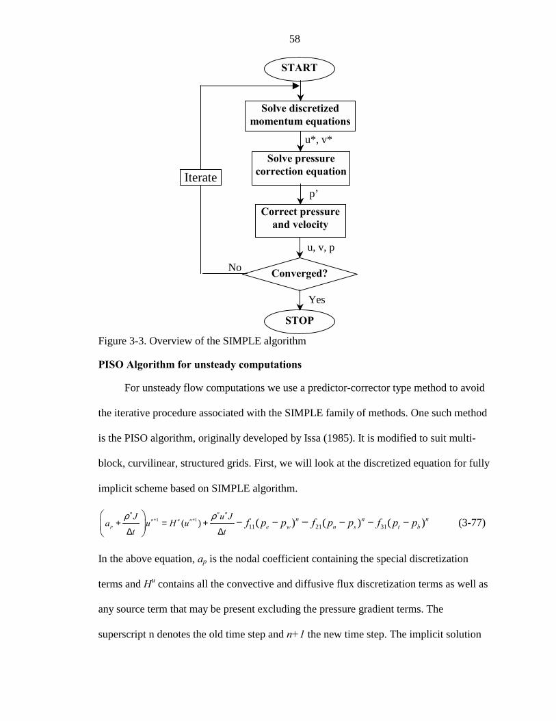
58
Figure 3-3. Overview of the SIMPLE algorithm
PISO Algorithm for unsteady computations
For unsteady flow computations we use a predictor-corrector type method to avoid
the iterative procedure associated with the SIMPLE family of methods. One such method
is the PISO algorithm, originally developed by Issa (1985). It is modified to suit multi-
block, curvilinear, structured grids. First, we will look at the discretized equation for fully
implicit scheme based on SIMPLE algorithm.
1 1
11 21 31( ) ( ) ( ) ( )n n n
n u n
P
n n ne w n s t b
J u Ja u H u
t tf p p f p p f p p+ ++ = +
∆ ∆
− − − − −
−ρ ρ (3-77)
In the above equation, ap is the nodal coefficient containing the special discretization
terms and Hu contains all the convective and diffusive flux discretization terms as well as
any source term that may be present excluding the pressure gradient terms. The
superscript n denotes the old time step and n+1 the new time step. The implicit solution
START
Solve discretized momentum equations
Solve pressure correction equation
Correct pressure and velocity
Converged?
STOP
No
Yes
Iterate
u*, v*
p’
u, v, p
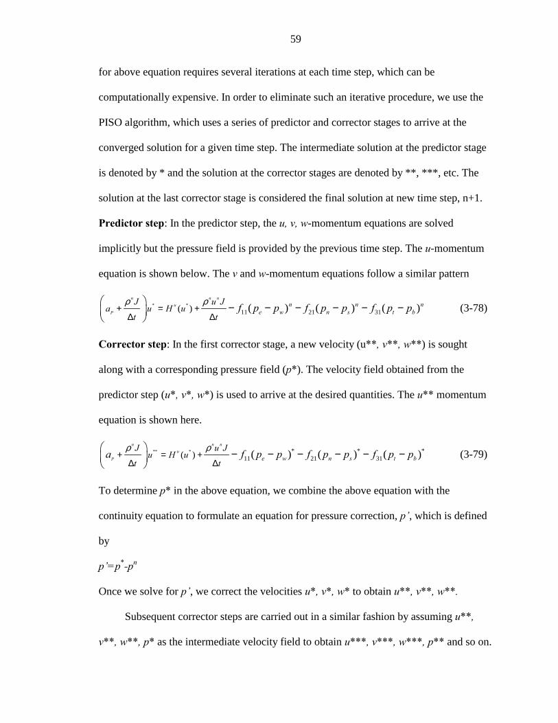
59
for above equation requires several iterations at each time step, which can be
computationally expensive. In order to eliminate such an iterative procedure, we use the
PISO algorithm, which uses a series of predictor and corrector stages to arrive at the
converged solution for a given time step. The intermediate solution at the predictor stage
is denoted by * and the solution at the corrector stages are denoted by **, ***, etc. The
solution at the last corrector stage is considered the final solution at new time step, n+1.
Predictor step: In the predictor step, the u, v, w-momentum equations are solved
implicitly but the pressure field is provided by the previous time step. The u-momentum
equation is shown below. The v and w-momentum equations follow a similar pattern
* *
11 21 31( ) ( ) ( ) ( )n n n
u
P
n n ne w n s t b
J u Ja u H u
t tf p p f p p f p p+ = +
∆ ∆
− − − − − −
ρ ρ (3-78)
Corrector step: In the first corrector stage, a new velocity (u**, v**, w**) is sought
along with a corresponding pressure field (p*). The velocity field obtained from the
predictor step (u*, v*, w*) is used to arrive at the desired quantities. The u** momentum
equation is shown here.
** * * * *11 21 31( ) ( ) ( ) ( )
n n nu
P e w n s t bJ u J
u H ut t
a f p p f p p f p p+ = +∆ ∆
− − − − − −
ρ ρ (3-79)
To determine p* in the above equation, we combine the above equation with the
continuity equation to formulate an equation for pressure correction, p, which is defined
by
p=p*-pn
Once we solve for p, we correct the velocities u*, v*, w* to obtain u**, v**, w**.
Subsequent corrector steps are carried out in a similar fashion by assuming u**,
v**, w**, p* as the intermediate velocity field to obtain u***, v***, w***, p** and so on.
60
A total of four corrector stages were used to arrive at the final solution at the new time
level, n+1. The PISO algorithm, being a semi-implicit method, is limited by the choice of
time step based of CFL number, which is defined as follows
u tCFLx
∆=∆
where u is the free stream velocity, ∆x is the grid spacing. Time step size is chosen based
on free stream velocity and grid spacing so as to obtain a CFL number with an O(1)
magnitude. An overview of the PISO algorithm is shown in Figure 3-4. A detailed
procedure of the algorithm can be found in Thakur et al. (2002).
Updating Jacobian values for moving boundary treatment
While formulating the above-mentioned solver for the moving boundary problem,
we need to make sure that the geometric conservation law is satisfied. This is ensured by
updating the Jacobians in a consistent fashion. The equation that needs to be satisfied is
re-written here for convenience
( ) ( ) ( ) 0t t t tJ ξ η ζξ η ζ+ + + = (3-21)
We will now look at how to calculate the Jacobian values in a consistent fashion. In this
regard, we will implement four different time-integration schemes for evaluating the
Jacobian values: first order implicit scheme, first order time-averaged scheme, second
order implicit scheme and a second order time-averaged scheme. The formulation for the
different GCL schemes is as follows.
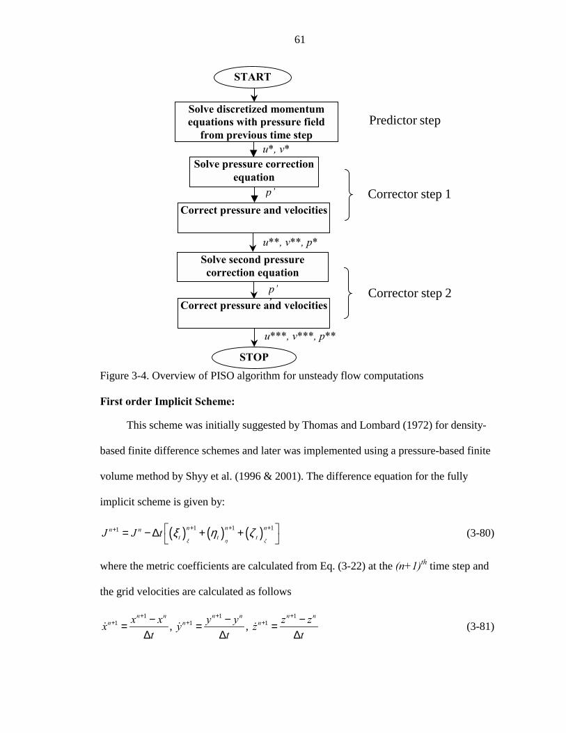
61
Figure 3-4. Overview of PISO algorithm for unsteady flow computations
First order Implicit Scheme:
This scheme was initially suggested by Thomas and Lombard (1972) for density-
based finite difference schemes and later was implemented using a pressure-based finite
volume method by Shyy et al. (1996 & 2001). The difference equation for the fully
implicit scheme is given by:
( ) ( ) ( )1 1 11 n n nn nt t tJ J t
ξ η ζξ η ζ+ + ++ = − ∆ + +
(3-80)
where the metric coefficients are calculated from Eq. (3-22) at the (n+1)th time step and
the grid velocities are calculated as follows
1 1 11 1 1, ,
n n n n n nn n nx x y y z zx y z
t t t
+ + ++ + +− − −= = =
∆ ∆ ∆! ! ! (3-81)
Predictor step
Corrector step 1
Corrector step 2
START
Solve pressure correction equation
Correct pressure and velocities
STOP
Correct pressure and velocities
Solve second pressure correction equation
Solve discretized momentum equations with pressure field
from previous time step
u**, v**, p*
u*, v*
p
p’
u***, v***, p**
62
First-order time-averaged scheme:
It was suggested (Farhat et al., 2001) that a time-averaged evaluation of the metric
terms leads to a more consistent evaluation of the Jacobian especially when the time step
is large. Hence, we re-formulate the governing equation (Eq. (3-21)) by time-averaging
the evaluation of metrics over more than one mesh configuration as opposed to
evaluation of metrics on a single mesh configuration (Eq. (3-80)). It can be written as
follows:
( ) ( ) ( )1 1 1 1
2 2 2 0n n
n n nt t t
J Jt ξ η ζ
ξ η ζ+
+ + +− + + + = ∆ (3-82)
The metric terms are computed as follows:
( ) ( ) ( )
( ) ( ) ( )
( ) ( ) ( )
1 12
1 12
1 12
121212
n n nt t t
n n nt t t
n n nt t t
ξ ξ ξ
ξ ξ ξ
ξ ξ ξ
ξ ξ ξ
η η η
ζ ζ ζ
+ +
+ +
+ +
= +
= +
= +
As can be seen from the above expression that the metrics are evaluated at a mesh
configuration, which is in between the mesh configurations at tn and tn+1. The grid
velocities for the metric term are evaluated as follows:
1 1 11 1 12 2 2, ,
n n n n n nn n nx x y y z zx y zt t t
+ + ++ + +− − −= = =∆ ∆ ∆
! ! ! (3-83)
Second order implicit scheme
The difference equation for a second order implicit scheme (3-point backward), as
suggested by Koobus and Farhat (1999) is used here. For structured meshes, it can be
written as
63
( ) ( ) ( )1 1
1 1 1
3 122 2 0
n n n
n n nt t t
J J J
t ξ η ζξ η ζ
+ −
+ + +− +
+ + + = ∆
(3-84)
Here, the metrics are evaluated in a similar fashion to the one used for first order implicit
scheme at the (n+1)th grid configuration. The grid velocity is also calculated in a similar
fashion as given by Eq. (3-81).
Second order time-averaged evaluation of Jacobian
Here we use a time-averaged procedure to evaluate the fluxes. Koobus and Farhat
(1999) employed such a procedure for unstructured meshes and we extend such a scheme
to a structured mesh here. The scheme can be written as follows.
( ) ( ) ( )
( ) ( ) ( )
1 11 1 12 2 2
1 1 12 2 2
3 12 12 221 02
n n n
n n nt t t
n n nt t t
J J J
t ξ η ζ
ξ η ζ
ξ η ζ
ξ η ζ
+ −
+ + +
− − −
− + + + + ∆ + + + =
(3-85)
where
( ) ( ) ( ) ( ) ( ) ( )
( ) ( ) ( ) ( ) ( ) ( )
( ) ( ) ( ) ( ) ( ) ( )
1 11 12 2
1 11 12 2
1 11 12 2
1 1;2 21 1;2 21 1;2 2
n n n n n nt t t t t t
n n n n n nt t t t t t
n n n n n nt t t t t t
ξ ξ ξ ξ ξ ξ
ξ ξ ξ ξ ξ ξ
ξ ξ ξ ξ ξ ξ
ξ ξ ξ ξ ξ ξ
η η η η η η
ζ ζ ζ ζ ζ ζ
+ + − −
+ + − −
+ + − −
= + = +
= + = +
= + = +
(3-86)
Here, the averaging is done in between configurations [tn, tn+1] and [tn, tn-1] and the mesh
velocities for each of these metric terms are evaluated as follows:
1 1 11 1 12 2 2
1 1 11 1 12 2 2
, ,
, ,
n n n n n nn n n
n n n n n nn n n
x x y y z zx y zt t t
x x y y z zx y zt t t
+ + ++ + +
− − −− − −
− − −= = =∆ ∆ ∆− − −= = =∆ ∆ ∆
! ! !
! ! ! (3-87)
64
As can be seen from the above equations that we need three different mesh
configurations to arrive at this scheme. All of the above-mentioned schemes will be
implemented using several test cases to arrive at the appropriate scheme for aeroelastic
computations.
Newmark Integration Method for Structure Solver
In this section, the numerical procedure used to solve the structure equations of
motion is presented. The equations of motion of the structure, written for the individual
modes, can be written in a generalized form for any particular mode as follows
22z z z rξω ω+ + =!! !! (3-88)
Equation (3-88), written at a time t+∆t, reads as follows
22t t t t t t t tz z z rξω ω+∆ +∆ +∆ +∆+ + =!! !! (3-89)
In the above expression, ξ, ω, and t tr +∆ are known before hand. The task is to evaluate the
displacement, velocity and acceleration at the time t+∆t. The following expressions for
velocity and displacement are formulated at time t+∆t first as a function of acceleration at
t+∆t and displacement, velocity and acceleration from previous time level t.
[ ](1 )t t t t t tz z tz zδ δ+∆ +∆= ∆+ − +! ! !! !! (3-90)
212( )t t t t t t tz z z t tz zα α+∆ +∆
= + ∆ ∆ + − +! !! !! (3-91)
where, α and δ are parameters that are chosen based on desired stability and accuracy.
For the Newmark scheme to be unconditionally stable, values of 0.25 and 0.5 are chosen
for α and δ, respectively.
65
Substituting Eqs. (3-90) and (3-91) into Eq. (3-89) and solving for t tz +∆!! and then
using Eqs. (3-90) and (3-91) to calculate t tz +∆! and t tz +∆ , the following relation can be
established for displacement, velocity and acceleration.
t t t
t t t t t
t t t
z zz z rz z
+∆
+∆ +∆
+∆
= +
A L!! !!! ! (3-92)
where
[ ][ ] ( )
12 2
12
2 1 12 2
1 1( ) 2(1 ) ( 2 ) ( )
11 ( ) 2(1 ) 1 2 ( )
( ) 2(1 ) 1 2 (1 )
t t
tt
t t
α β δ κ β κ β
δ α δβ δ δκ βδ δκ δβ
α α α β δ ακ αβ ακ α β
− − − − − − − ∆ ∆ = ∆ − − − − − − − − ∆ ∆ − − − − − ∆ − − −
A (3-93)
2 2
2
2
t
t
βωβδ
ωαβω
∆ = ∆
L (3-94)
1
2 2
1 2 ; t t t
ξδ ξββ α κω ω ω
− = + + = ∆ ∆ ∆

66
CHAPTER 4 COMPUTATIONAL PROCEDURE AND CODE VALIDATION
In this chapter, the computational procedure for performing fluid-structure
interaction computations will be discussed in depth. The computational setup for the test
case that is used to carry out computations will be shown as well. We also present
validation results associated with several modules of the computational aeroelasticity
model.
Computational Procedure
The overall procedure for carrying out computational aeroelastic computations can
be divided into the following major steps.
1. Constructing the geometry for aeroelastic computations and also to supply appropriate boundary conditions and initial conditions.
2. Perform steady state CFD computation to obtain initial guess for starting coupled computations.
3. Perform unsteady CFD computations using steady state result as initial guess and obtain necessary aerodynamic forces on the surface of the wing.
4. Interpolate aerodynamic forces onto the structural mesh.
5. Perform CSD computation to obtain the deformation of the geometry
6. Extrapolate the displacements onto CFD surface grid.
7. Re-mesh CFD grid based on the deformation obtained from the CSD calculations using the moving boundary module.
8. Repeat steps 3-7 using current solution as the initial guess for the subsequent steps.
Now we will take a closer look at the above-mentioned steps along with the grid
generation details, interpolation/extrapolation schemes used.
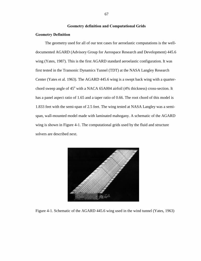
67
Geometry definition and Computational Grids
Geometry Definition
The geometry used for all of our test cases for aeroelastic computations is the well-
documented AGARD (Advisory Group for Aerospace Research and Development) 445.6
wing (Yates, 1987). This is the first AGARD standard aeroelastic configuration. It was
first tested in the Transonic Dynamics Tunnel (TDT) at the NASA Langley Research
Center (Yates et al. 1963). The AGARD 445.6 wing is a swept back wing with a quarter-
chord sweep angle of 45o with a NACA 65A004 airfoil (4% thickness) cross-section. It
has a panel aspect ratio of 1.65 and a taper ratio of 0.66. The root chord of this model is
1.833 feet with the semi-span of 2.5 feet. The wing tested at NASA Langley was a semi-
span, wall-mounted model made with laminated mahogany. A schematic of the AGARD
wing is shown in Figure 4-1. The computational grids used by the fluid and structure
solvers are described next.
Figure 4-1. Schematic of the AGARD 445.6 wing used in the wind tunnel (Yates, 1963)
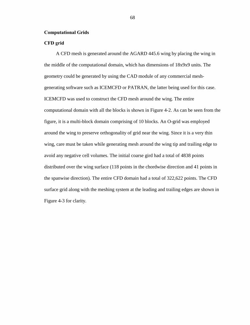
68
Computational Grids
CFD grid
A CFD mesh is generated around the AGARD 445.6 wing by placing the wing in
the middle of the computational domain, which has dimensions of 18x9x9 units. The
geometry could be generated by using the CAD module of any commercial mesh-
generating software such as ICEMCFD or PATRAN, the latter being used for this case.
ICEMCFD was used to construct the CFD mesh around the wing. The entire
computational domain with all the blocks is shown in Figure 4-2. As can be seen from the
figure, it is a multi-block domain comprising of 10 blocks. An O-grid was employed
around the wing to preserve orthogonality of grid near the wing. Since it is a very thin
wing, care must be taken while generating mesh around the wing tip and trailing edge to
avoid any negative cell volumes. The initial coarse gird had a total of 4838 points
distributed over the wing surface (118 points in the chordwise direction and 41 points in
the spanwise direction). The entire CFD domain had a total of 322,622 points. The CFD
surface grid along with the meshing system at the leading and trailing edges are shown in
Figure 4-3 for clarity.
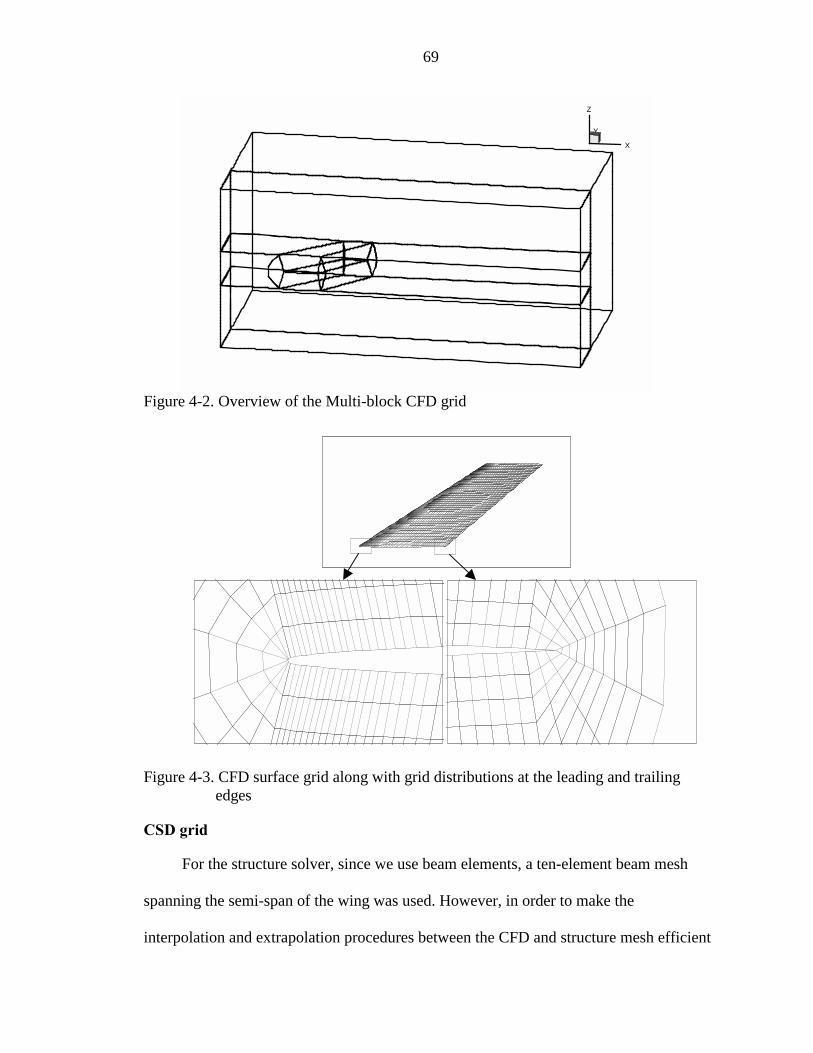
69
Figure 4-2. Overview of the Multi-block CFD grid
Figure 4-3. CFD surface grid along with grid distributions at the leading and trailing edges
CSD grid
For the structure solver, since we use beam elements, a ten-element beam mesh
spanning the semi-span of the wing was used. However, in order to make the
interpolation and extrapolation procedures between the CFD and structure mesh efficient
Y
X
Z
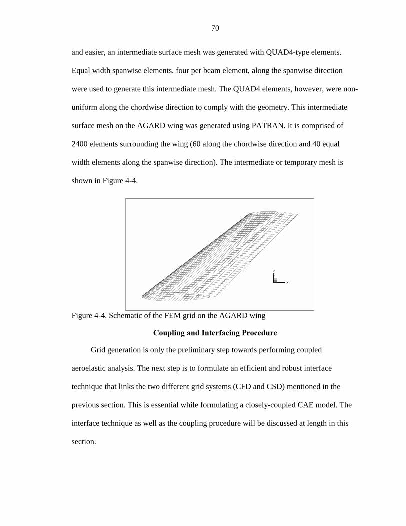
70
and easier, an intermediate surface mesh was generated with QUAD4-type elements.
Equal width spanwise elements, four per beam element, along the spanwise direction
were used to generate this intermediate mesh. The QUAD4 elements, however, were non-
uniform along the chordwise direction to comply with the geometry. This intermediate
surface mesh on the AGARD wing was generated using PATRAN. It is comprised of
2400 elements surrounding the wing (60 along the chordwise direction and 40 equal
width elements along the spanwise direction). The intermediate or temporary mesh is
shown in Figure 4-4.
Figure 4-4. Schematic of the FEM grid on the AGARD wing
Coupling and Interfacing Procedure
Grid generation is only the preliminary step towards performing coupled
aeroelastic analysis. The next step is to formulate an efficient and robust interface
technique that links the two different grid systems (CFD and CSD) mentioned in the
previous section. This is essential while formulating a closely-coupled CAE model. The
interface technique as well as the coupling procedure will be discussed at length in this
section.
X
YZ
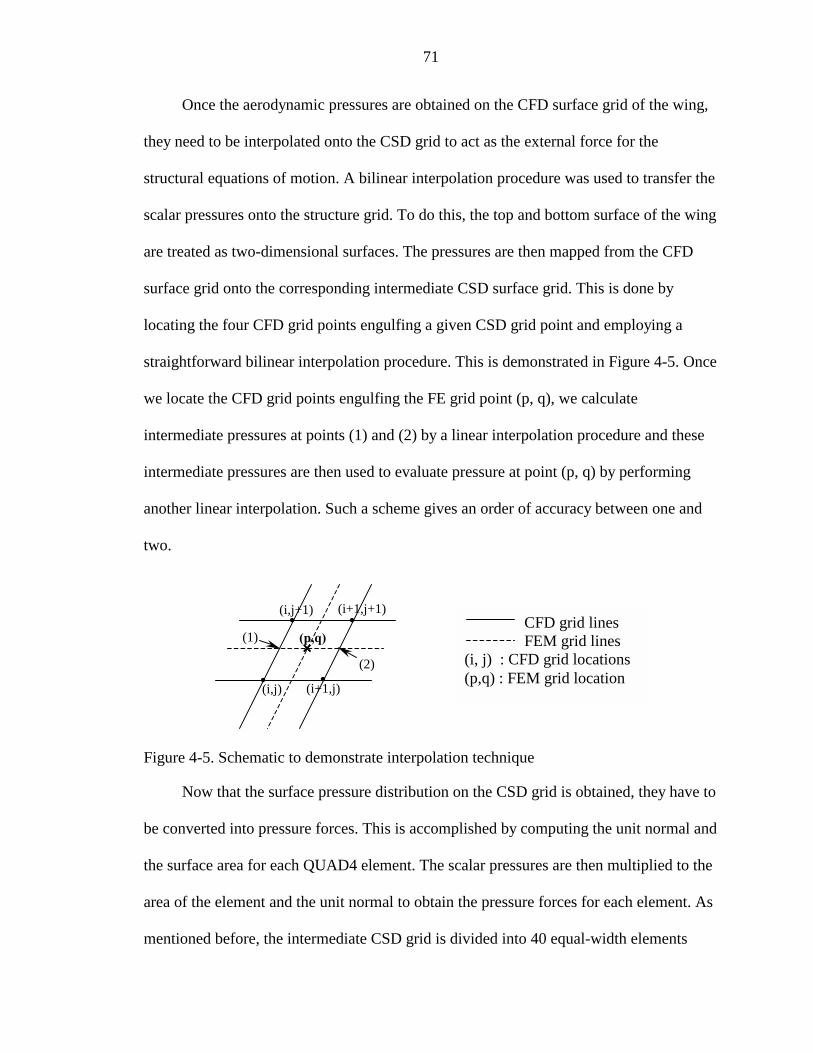
71
Once the aerodynamic pressures are obtained on the CFD surface grid of the wing,
they need to be interpolated onto the CSD grid to act as the external force for the
structural equations of motion. A bilinear interpolation procedure was used to transfer the
scalar pressures onto the structure grid. To do this, the top and bottom surface of the wing
are treated as two-dimensional surfaces. The pressures are then mapped from the CFD
surface grid onto the corresponding intermediate CSD surface grid. This is done by
locating the four CFD grid points engulfing a given CSD grid point and employing a
straightforward bilinear interpolation procedure. This is demonstrated in Figure 4-5. Once
we locate the CFD grid points engulfing the FE grid point (p, q), we calculate
intermediate pressures at points (1) and (2) by a linear interpolation procedure and these
intermediate pressures are then used to evaluate pressure at point (p, q) by performing
another linear interpolation. Such a scheme gives an order of accuracy between one and
two.
Figure 4-5. Schematic to demonstrate interpolation technique
Now that the surface pressure distribution on the CSD grid is obtained, they have to
be converted into pressure forces. This is accomplished by computing the unit normal and
the surface area for each QUAD4 element. The scalar pressures are then multiplied to the
area of the element and the unit normal to obtain the pressure forces for each element. As
mentioned before, the intermediate CSD grid is divided into 40 equal-width elements
• •
• •
×××× (p,q)
(i,j)
(i,j+1)
(i+1,j)
(i+1,j+1)
(1)
(2)
CFD grid lines FEM grid lines (i, j) : CFD grid locations (p,q) : FEM grid location
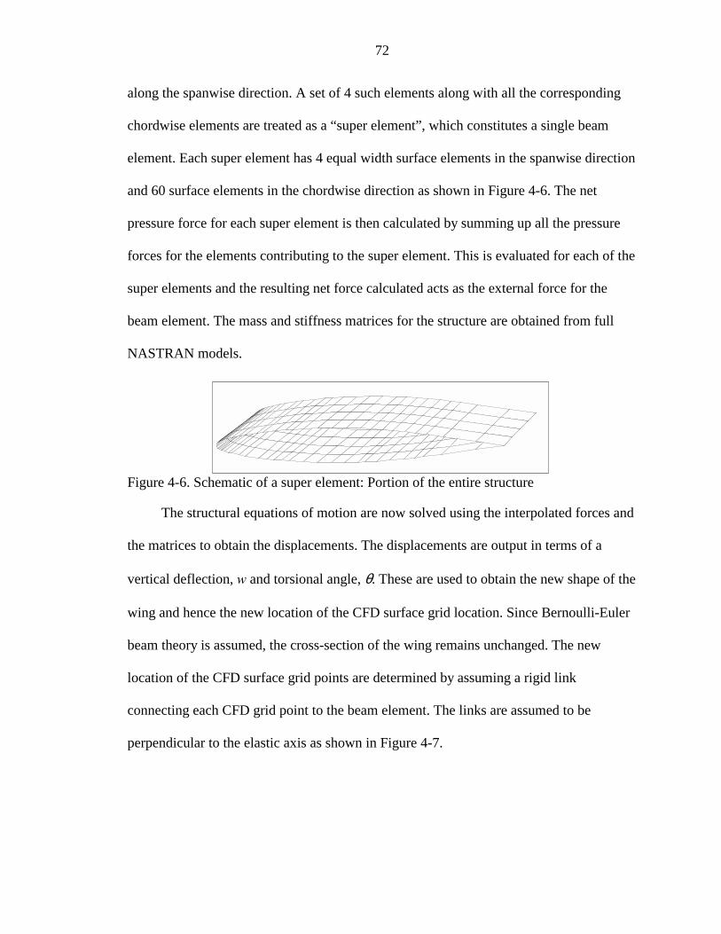
72
along the spanwise direction. A set of 4 such elements along with all the corresponding
chordwise elements are treated as a “super element”, which constitutes a single beam
element. Each super element has 4 equal width surface elements in the spanwise direction
and 60 surface elements in the chordwise direction as shown in Figure 4-6. The net
pressure force for each super element is then calculated by summing up all the pressure
forces for the elements contributing to the super element. This is evaluated for each of the
super elements and the resulting net force calculated acts as the external force for the
beam element. The mass and stiffness matrices for the structure are obtained from full
NASTRAN models.
Figure 4-6. Schematic of a super element: Portion of the entire structure
The structural equations of motion are now solved using the interpolated forces and
the matrices to obtain the displacements. The displacements are output in terms of a
vertical deflection, w and torsional angle, θ. These are used to obtain the new shape of the
wing and hence the new location of the CFD surface grid location. Since Bernoulli-Euler
beam theory is assumed, the cross-section of the wing remains unchanged. The new
location of the CFD surface grid points are determined by assuming a rigid link
connecting each CFD grid point to the beam element. The links are assumed to be
perpendicular to the elastic axis as shown in Figure 4-7.
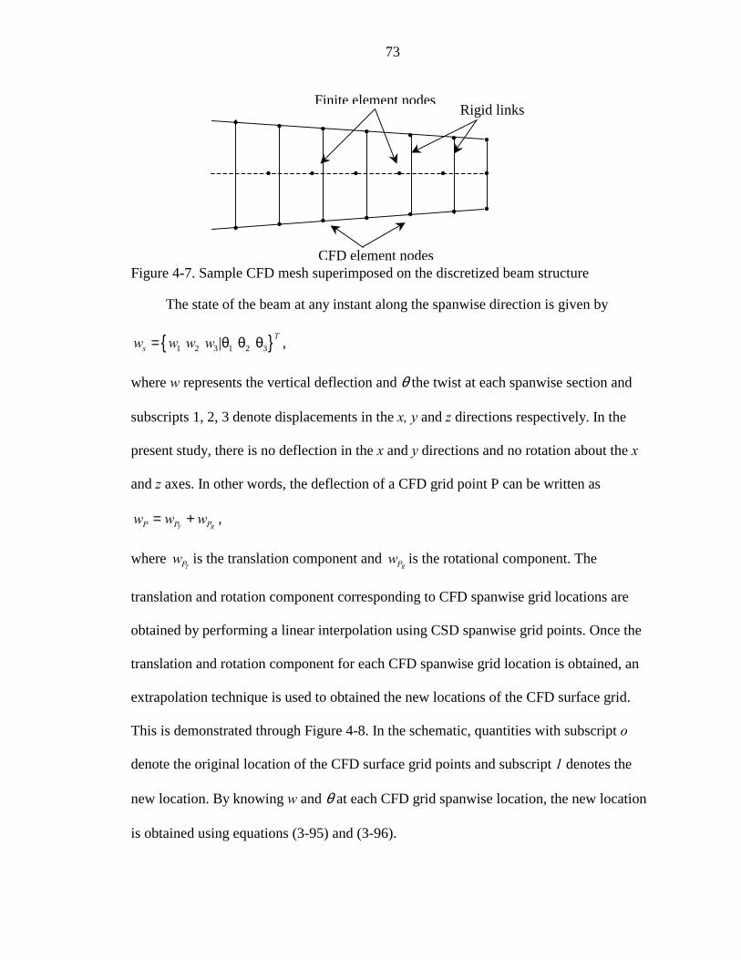
73
Figure 4-7. Sample CFD mesh superimposed on the discretized beam structure
The state of the beam at any instant along the spanwise direction is given by
1 2 3 1 2 3 | Tsw w w w= θ θ θ ,
where w represents the vertical deflection and θ the twist at each spanwise section and
subscripts 1, 2, 3 denote displacements in the x, y and z directions respectively. In the
present study, there is no deflection in the x and y directions and no rotation about the x
and z axes. In other words, the deflection of a CFD grid point P can be written as
T RP P Pw w w= + ,
where TPw is the translation component and
RPw is the rotational component. The
translation and rotation component corresponding to CFD spanwise grid locations are
obtained by performing a linear interpolation using CSD spanwise grid points. Once the
translation and rotation component for each CFD spanwise grid location is obtained, an
extrapolation technique is used to obtained the new locations of the CFD surface grid.
This is demonstrated through Figure 4-8. In the schematic, quantities with subscript o
denote the original location of the CFD surface grid points and subscript 1 denotes the
new location. By knowing w and θ at each CFD grid spanwise location, the new location
is obtained using equations (3-95) and (3-96).
• • • • • ••
• • • • • •
• • • • • ••
Finite element nodes
CFD element nodes
Rigid links
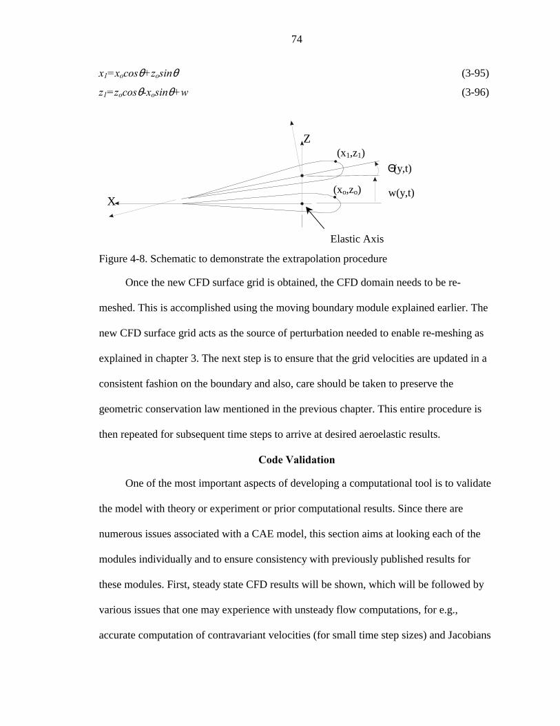
74
x1=xocosθ+zosinθ (3-95)
z1=zocosθ-xosinθ+w (3-96)
Figure 4-8. Schematic to demonstrate the extrapolation procedure
Once the new CFD surface grid is obtained, the CFD domain needs to be re-
meshed. This is accomplished using the moving boundary module explained earlier. The
new CFD surface grid acts as the source of perturbation needed to enable re-meshing as
explained in chapter 3. The next step is to ensure that the grid velocities are updated in a
consistent fashion on the boundary and also, care should be taken to preserve the
geometric conservation law mentioned in the previous chapter. This entire procedure is
then repeated for subsequent time steps to arrive at desired aeroelastic results.
Code Validation
One of the most important aspects of developing a computational tool is to validate
the model with theory or experiment or prior computational results. Since there are
numerous issues associated with a CAE model, this section aims at looking each of the
modules individually and to ensure consistency with previously published results for
these modules. First, steady state CFD results will be shown, which will be followed by
various issues that one may experience with unsteady flow computations, for e.g.,
accurate computation of contravariant velocities (for small time step sizes) and Jacobians
Z
Xw(y,t)
Θ (y,t)
(xo,zo)
(x1,z1)
Elastic Axis
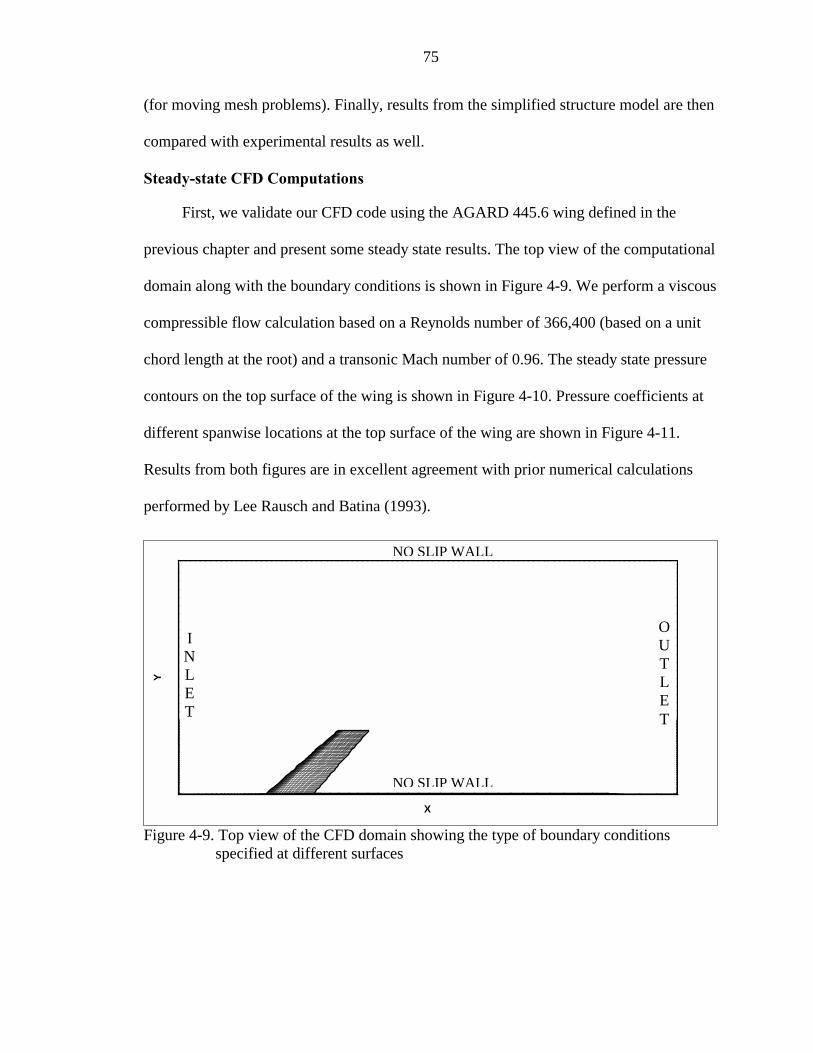
75
(for moving mesh problems). Finally, results from the simplified structure model are then
compared with experimental results as well.
Steady-state CFD Computations
First, we validate our CFD code using the AGARD 445.6 wing defined in the
previous chapter and present some steady state results. The top view of the computational
domain along with the boundary conditions is shown in Figure 4-9. We perform a viscous
compressible flow calculation based on a Reynolds number of 366,400 (based on a unit
chord length at the root) and a transonic Mach number of 0.96. The steady state pressure
contours on the top surface of the wing is shown in Figure 4-10. Pressure coefficients at
different spanwise locations at the top surface of the wing are shown in Figure 4-11.
Results from both figures are in excellent agreement with prior numerical calculations
performed by Lee Rausch and Batina (1993).
Figure 4-9. Top view of the CFD domain showing the type of boundary conditions specified at different surfaces
X
Y
NO SLIP WALL
NO SLIP WALL
INLET
OUTLET
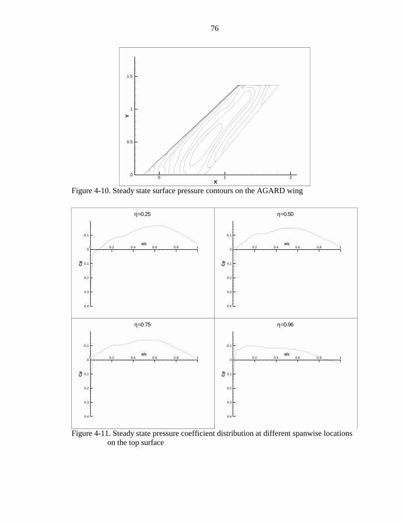
76
Figure 4-10. Steady state surface pressure contours on the AGARD wing
Figure 4-11. Steady state pressure coefficient distribution at different spanwise locations on the top surface
x/c
Cp
0 0.2 0.4 0.6 0.8 1
-0.1
0
0.1
0.2
0.3
0.4
η=0.25
x/c
Cp
0 0.2 0.4 0.6 0.8 1
-0.1
0
0.1
0.2
0.3
0.4
η=0.50
x/c
Cp
0 0.2 0.4 0.6 0.8 1
-0.1
0
0.1
0.2
0.3
0.4
η=0.96
x/c
Cp
0 0.2 0.4 0.6 0.8 1
-0.1
0
0.1
0.2
0.3
0.4
η=0.75
X
Y
0 1 20
0.5
1
1.5
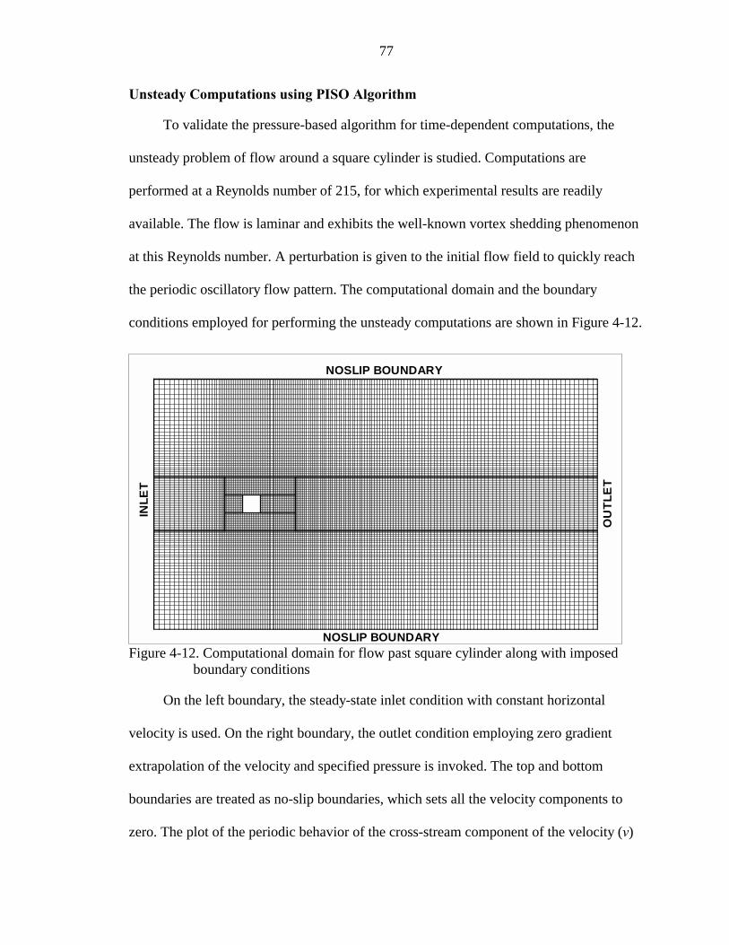
77
Unsteady Computations using PISO Algorithm
To validate the pressure-based algorithm for time-dependent computations, the
unsteady problem of flow around a square cylinder is studied. Computations are
performed at a Reynolds number of 215, for which experimental results are readily
available. The flow is laminar and exhibits the well-known vortex shedding phenomenon
at this Reynolds number. A perturbation is given to the initial flow field to quickly reach
the periodic oscillatory flow pattern. The computational domain and the boundary
conditions employed for performing the unsteady computations are shown in Figure 4-12.
Figure 4-12. Computational domain for flow past square cylinder along with imposed boundary conditions
On the left boundary, the steady-state inlet condition with constant horizontal
velocity is used. On the right boundary, the outlet condition employing zero gradient
extrapolation of the velocity and specified pressure is invoked. The top and bottom
boundaries are treated as no-slip boundaries, which sets all the velocity components to
zero. The plot of the periodic behavior of the cross-stream component of the velocity (v)
NOSLIP BOUNDARY
NOSLIP BOUNDARY
INLE
T
OU
TLE
T
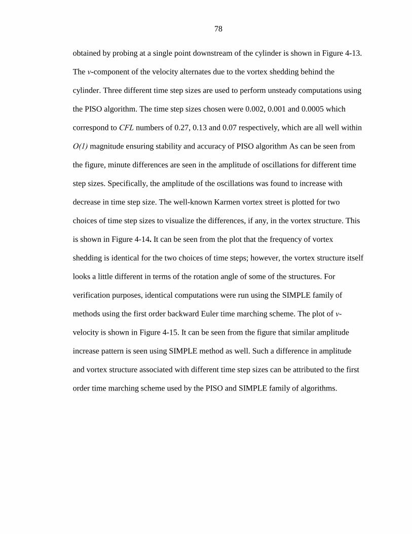
78
obtained by probing at a single point downstream of the cylinder is shown in Figure 4-13.
The v-component of the velocity alternates due to the vortex shedding behind the
cylinder. Three different time step sizes are used to perform unsteady computations using
the PISO algorithm. The time step sizes chosen were 0.002, 0.001 and 0.0005 which
correspond to CFL numbers of 0.27, 0.13 and 0.07 respectively, which are all well within
O(1) magnitude ensuring stability and accuracy of PISO algorithm As can be seen from
the figure, minute differences are seen in the amplitude of oscillations for different time
step sizes. Specifically, the amplitude of the oscillations was found to increase with
decrease in time step size. The well-known Karmen vortex street is plotted for two
choices of time step sizes to visualize the differences, if any, in the vortex structure. This
is shown in Figure 4-14. It can be seen from the plot that the frequency of vortex
shedding is identical for the two choices of time steps; however, the vortex structure itself
looks a little different in terms of the rotation angle of some of the structures. For
verification purposes, identical computations were run using the SIMPLE family of
methods using the first order backward Euler time marching scheme. The plot of v-
velocity is shown in Figure 4-15. It can be seen from the figure that similar amplitude
increase pattern is seen using SIMPLE method as well. Such a difference in amplitude
and vortex structure associated with different time step sizes can be attributed to the first
order time marching scheme used by the PISO and SIMPLE family of algorithms.
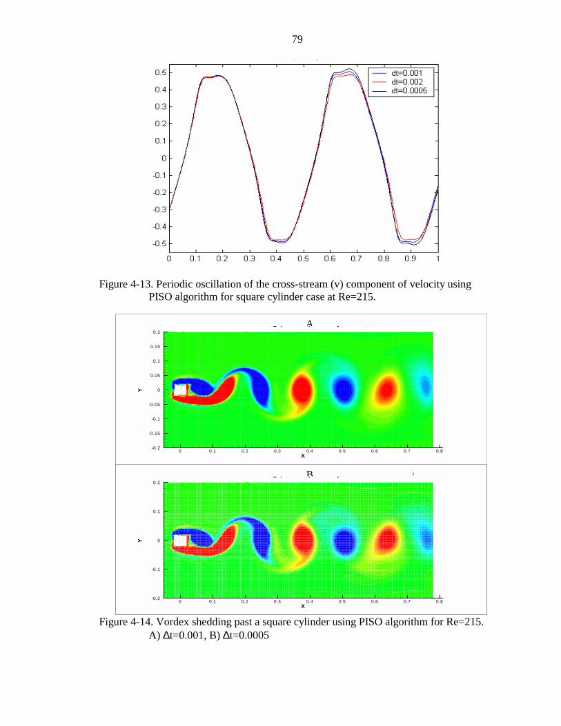
79
Figure 4-13. Periodic oscillation of the cross-stream (v) component of velocity using PISO algorithm for square cylinder case at Re=215.
Figure 4-14. Vordex shedding past a square cylinder using PISO algorithm for Re=215. A) ∆t=0.001, B) ∆t=0.0005
X
Y
0 0.1 0.2 0.3 0.4 0.5 0.6 0.7 0.8-0.2
-0.1
0
0.1
0.2
Vortex shedding past square cylinder, Dt=0.0005
X
Y
0 0.1 0.2 0.3 0.4 0.5 0.6 0.7 0.8-0.2
-0.15
-0.1
-0.05
0
0.05
0.1
0.15
0.2
Vortex shedding past square cylinder, Dt=0.002A
B
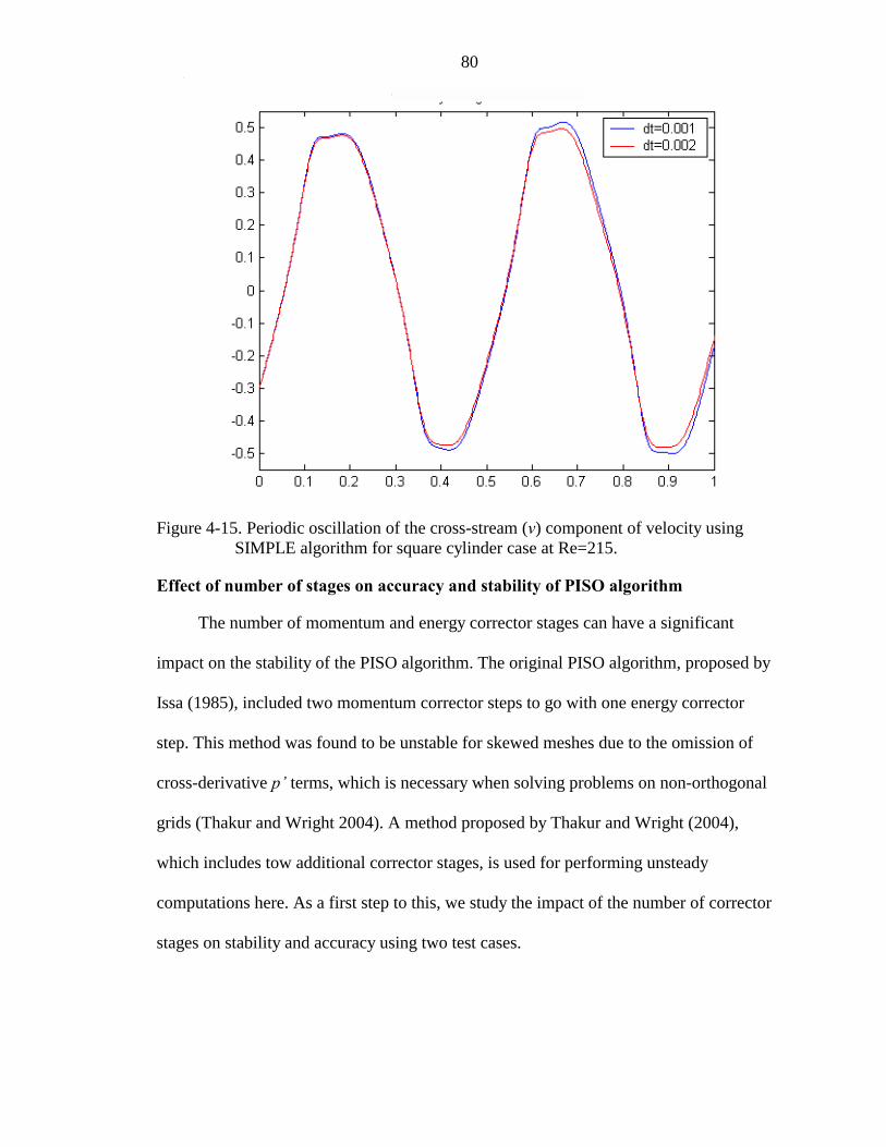
80
Figure 4-15. Periodic oscillation of the cross-stream (v) component of velocity using SIMPLE algorithm for square cylinder case at Re=215.
Effect of number of stages on accuracy and stability of PISO algorithm
The number of momentum and energy corrector stages can have a significant
impact on the stability of the PISO algorithm. The original PISO algorithm, proposed by
Issa (1985), included two momentum corrector steps to go with one energy corrector
step. This method was found to be unstable for skewed meshes due to the omission of
cross-derivative p terms, which is necessary when solving problems on non-orthogonal
grids (Thakur and Wright 2004). A method proposed by Thakur and Wright (2004),
which includes tow additional corrector stages, is used for performing unsteady
computations here. As a first step to this, we study the impact of the number of corrector
stages on stability and accuracy using two test cases.
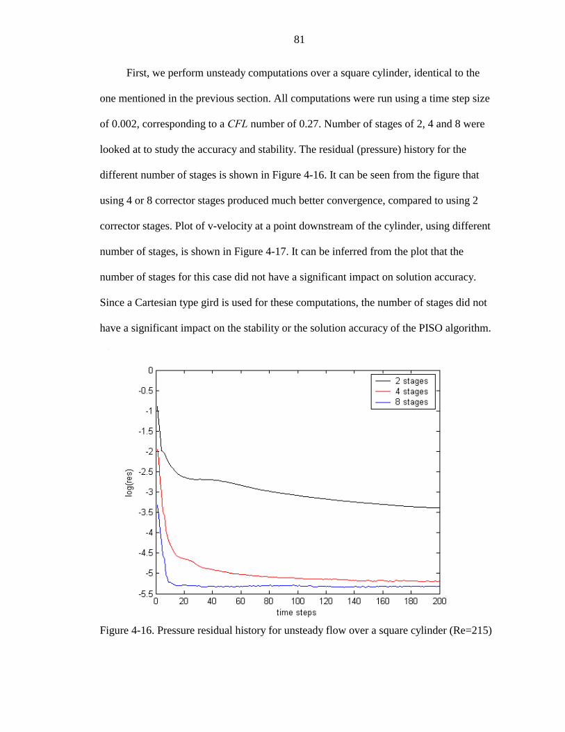
81
First, we perform unsteady computations over a square cylinder, identical to the
one mentioned in the previous section. All computations were run using a time step size
of 0.002, corresponding to a CFL number of 0.27. Number of stages of 2, 4 and 8 were
looked at to study the accuracy and stability. The residual (pressure) history for the
different number of stages is shown in Figure 4-16. It can be seen from the figure that
using 4 or 8 corrector stages produced much better convergence, compared to using 2
corrector stages. Plot of v-velocity at a point downstream of the cylinder, using different
number of stages, is shown in Figure 4-17. It can be inferred from the plot that the
number of stages for this case did not have a significant impact on solution accuracy.
Since a Cartesian type gird is used for these computations, the number of stages did not
have a significant impact on the stability or the solution accuracy of the PISO algorithm.
Figure 4-16. Pressure residual history for unsteady flow over a square cylinder (Re=215)
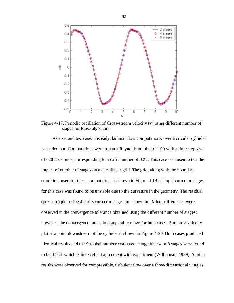
82
Figure 4-17. Periodic oscillation of Cross-stream velocity (v) using different number of stages for PISO algorithm
As a second test case, unsteady, laminar flow computations, over a circular cylinder
is carried out. Computations were run at a Reynolds number of 100 with a time step size
of 0.002 seconds, corresponding to a CFL number of 0.27. This case is chosen to test the
impact of number of stages on a curvilinear grid. The grid, along with the boundary
condition, used for these computations is shown in Figure 4-18. Using 2 corrector stages
for this case was found to be unstable due to the curvature in the geometry. The residual
(pressure) plot using 4 and 8 corrector stages are shown in . Minor differences were
observed in the convergence tolerance obtained using the different number of stages;
however, the convergence rate is in comparable range for both cases. Similar v-velocity
plot at a point downstream of the cylinder is shown in Figure 4-20. Both cases produced
identical results and the Strouhal number evaluated using either 4 or 8 stages were found
to be 0.164, which is in excellent agreement with experiment (Williamson 1989). Similar
results were observed for compressible, turbulent flow over a three-dimensional wing as
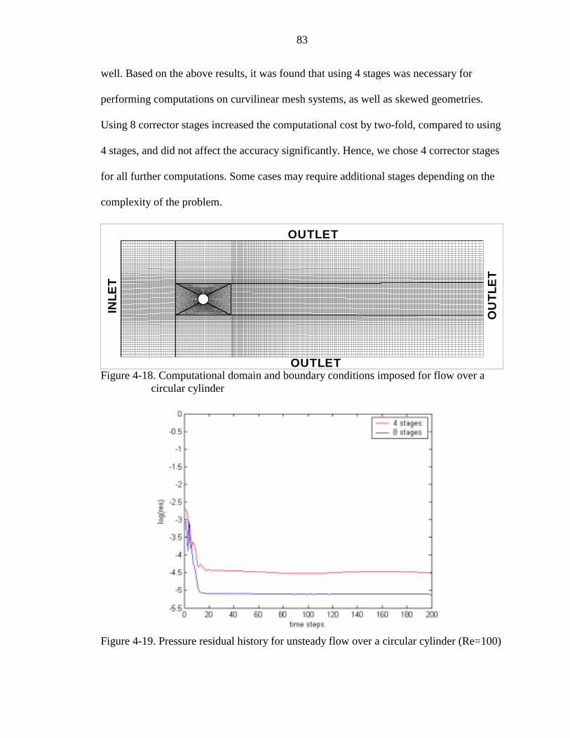
83
well. Based on the above results, it was found that using 4 stages was necessary for
performing computations on curvilinear mesh systems, as well as skewed geometries.
Using 8 corrector stages increased the computational cost by two-fold, compared to using
4 stages, and did not affect the accuracy significantly. Hence, we chose 4 corrector stages
for all further computations. Some cases may require additional stages depending on the
complexity of the problem.
Figure 4-18. Computational domain and boundary conditions imposed for flow over a circular cylinder
Figure 4-19. Pressure residual history for unsteady flow over a circular cylinder (Re=100)
OUTLET
OUTLET
INLE
T
OU
TLE
T
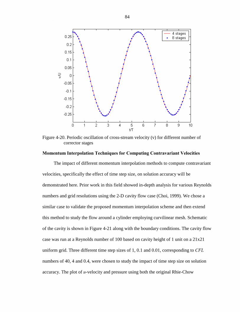
84
Figure 4-20. Periodic oscillation of cross-stream velocity (v) for different number of corrector stages
Momentum Interpolation Techniques for Computing Contravariant Velocities
The impact of different momentum interpolation methods to compute contravariant
velocities, specifically the effect of time step size, on solution accuracy will be
demonstrated here. Prior work in this field showed in-depth analysis for various Reynolds
numbers and grid resolutions using the 2-D cavity flow case (Choi, 1999). We chose a
similar case to validate the proposed momentum interpolation scheme and then extend
this method to study the flow around a cylinder employing curvilinear mesh. Schematic
of the cavity is shown in Figure 4-21 along with the boundary conditions. The cavity flow
case was run at a Reynolds number of 100 based on cavity height of 1 unit on a 21x21
uniform grid. Three different time step sizes of 1, 0.1 and 0.01, corresponding to CFL
numbers of 40, 4 and 0.4, were chosen to study the impact of time step size on solution
accuracy. The plot of u-velocity and pressure using both the original Rhie-Chow
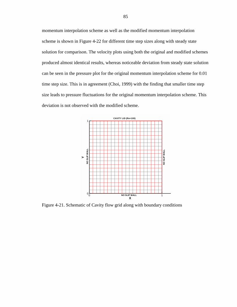
85
momentum interpolation scheme as well as the modified momentum interpolation
scheme is shown in Figure 4-22 for different time step sizes along with steady state
solution for comparison. The velocity plots using both the original and modified schemes
produced almost identical results, whereas noticeable deviation from steady state solution
can be seen in the pressure plot for the original momentum interpolation scheme for 0.01
time step size. This is in agreement (Choi, 1999) with the finding that smaller time step
size leads to pressure fluctuations for the original momentum interpolation scheme. This
deviation is not observed with the modified scheme.
Figure 4-21. Schematic of Cavity flow grid along with boundary conditions X
Y
0 10
1CAVITY LID (Re=100)
NO SLIP WALL
NO
SLI
PW
ALL
NO
SLI
PW
ALL
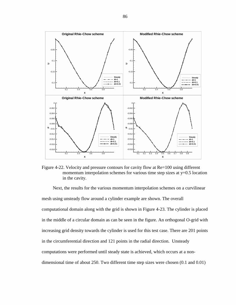
86
Figure 4-22. Velocity and pressure contours for cavity flow at Re=100 using different
momentum interpolation schemes for various time step sizes at y=0.5 location in the cavity.
Next, the results for the various momentum interpolation schemes on a curvilinear
mesh using unsteady flow around a cylinder example are shown. The overall
computational domain along with the grid is shown in Figure 4-23. The cylinder is placed
in the middle of a circular domain as can be seen in the figure. An orthogonal O-grid with
increasing grid density towards the cylinder is used for this test case. There are 201 points
in the circumferential direction and 121 points in the radial direction. Unsteady
computations were performed until steady state is achieved, which occurs at a non-
dimensional time of about 250. Two different time step sizes were chosen (0.1 and 0.01)
X
P
10 20 300
0.1
0.2Steady statedt=0.1dt=0.01
Original Rhie-Chow scheme
X
U
10 20
0
0.1
0.2
0.3
0.4
0.5
0.6
0.7
Steady statedt=0.1dt=0.01
Original Rhie-Chow scheme
X
U
10 20
0
0.1
0.2
0.3
0.4
0.5
0.6
0.7
Steady statedt=0.1dt=0.01
Modified Rhie-Chow scheme
X
P
10 20 300
0.1
0.2
Steady statedt=0.1dt=0.01
Modified Rhie-Chow scheme
X
P
0.2 0.4 0.6 0.8
-0.018
-0.016
-0.014
-0.012
-0.01
-0.008
-0.006
-0.004
-0.002
0
Steadydt=1dt=0.1dt=0.01
Original Rhie-Chow schemeX
U
0.2 0.4 0.6 0.8
-0.2
-0.15
-0.1
-0.05
Steadydt=1dt=0.1dt=0.01
Original Rhie-Chow scheme
X
U
0.2 0.4 0.6 0.8
-0.2
-0.15
-0.1
-0.05
Steadydt=1dt=0.1dt=0.01
Modified Rhie-Chow scheme
X
P
0.1 0.2 0.3 0.4 0.5 0.6 0.7 0.8 0.9
-0.018
-0.016
-0.014
-0.012
-0.01
-0.008
-0.006
-0.004
-0.002
0
Steadydt=1dt=0.1dt=0.01
Modified Rhie-Chow scheme
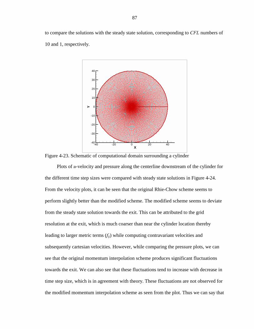
87
to compare the solutions with the steady state solution, corresponding to CFL numbers of
10 and 1, respectively.
Figure 4-23. Schematic of computational domain surrounding a cylinder
Plots of u-velocity and pressure along the centerline downstream of the cylinder for
the different time step sizes were compared with steady state solutions in Figure 4-24.
From the velocity plots, it can be seen that the original Rhie-Chow scheme seems to
perform slightly better than the modified scheme. The modified scheme seems to deviate
from the steady state solution towards the exit. This can be attributed to the grid
resolution at the exit, which is much coarser than near the cylinder location thereby
leading to larger metric terms (fij) while computing contravariant velocities and
subsequently cartesian velocities. However, while comparing the pressure plots, we can
see that the original momentum interpolation scheme produces significant fluctuations
towards the exit. We can also see that these fluctuations tend to increase with decrease in
time step size, which is in agreement with theory. These fluctuations are not observed for
the modified momentum interpolation scheme as seen from the plot. Thus we can say that
X
Y
-40 -20 0 20 40-40
-30
-20
-10
0
10
20
30
40
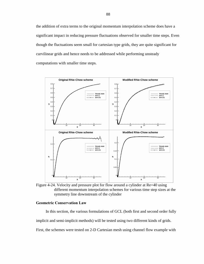
88
the addition of extra terms to the original momentum interpolation scheme does have a
significant impact in reducing pressure fluctuations observed for smaller time steps. Even
though the fluctuations seem small for cartesian type grids, they are quite significant for
curvilinear grids and hence needs to be addressed while performing unsteady
computations with smaller time steps.
Figure 4-24. Velocity and pressure plot for flow around a cylinder at Re=40 using different momentum interpolation schemes for various time step sizes at the symmetry line downstream of the cylinder
Geometric Conservation Law
In this section, the various formulations of GCL (both first and second order fully
implicit and semi-implicit methods) will be tested using two different kinds of grids.
First, the schemes were tested on 2-D Cartesian mesh using channel flow example with
X
P
0.1 0.2 0.3 0.4 0.5 0.6 0.7 0.8 0.9
-0.018
-0.016
-0.014
-0.012
-0.01
-0.008
-0.006
-0.004
-0.002
0
Steadydt=1dt=0.1dt=0.01
Modified Rhie-Chow schemeX
U
0.2 0.4 0.6 0.8
-0.2
-0.15
-0.1
-0.05
Steadydt=1dt=0.1dt=0.01
Modified Rhie-Chow scheme
X
U
0.2 0.4 0.6 0.8
-0.2
-0.15
-0.1
-0.05
Steadydt=1dt=0.1dt=0.01
Original Rhie-Chow scheme
X
P
0.2 0.4 0.6 0.8
-0.018
-0.016
-0.014
-0.012
-0.01
-0.008
-0.006
-0.004
-0.002
0
Steadydt=1dt=0.1dt=0.01
Original Rhie-Chow scheme
X
P
10 20 300
0.1
0.2Steady statedt=0.1dt=0.01
Original Rhie-Chow scheme
X
P
10 20 300
0.05
0.1
0.15
0.2
Steady statedt=0.1dt=0.01
Modified Rhie-Chow scheme
X
U
10 20 30
0
0.1
0.2
0.3
0.4
0.5
0.6
0.7
0.8
Steady statedt=0.1dt=0.01
Modified Rhie-Chow scheme
X
U
10 20 30
0
0.1
0.2
0.3
0.4
0.5
0.6
0.7
0.8
Steady statedt=0.1dt=0.01
Original Rhie-Chow scheme
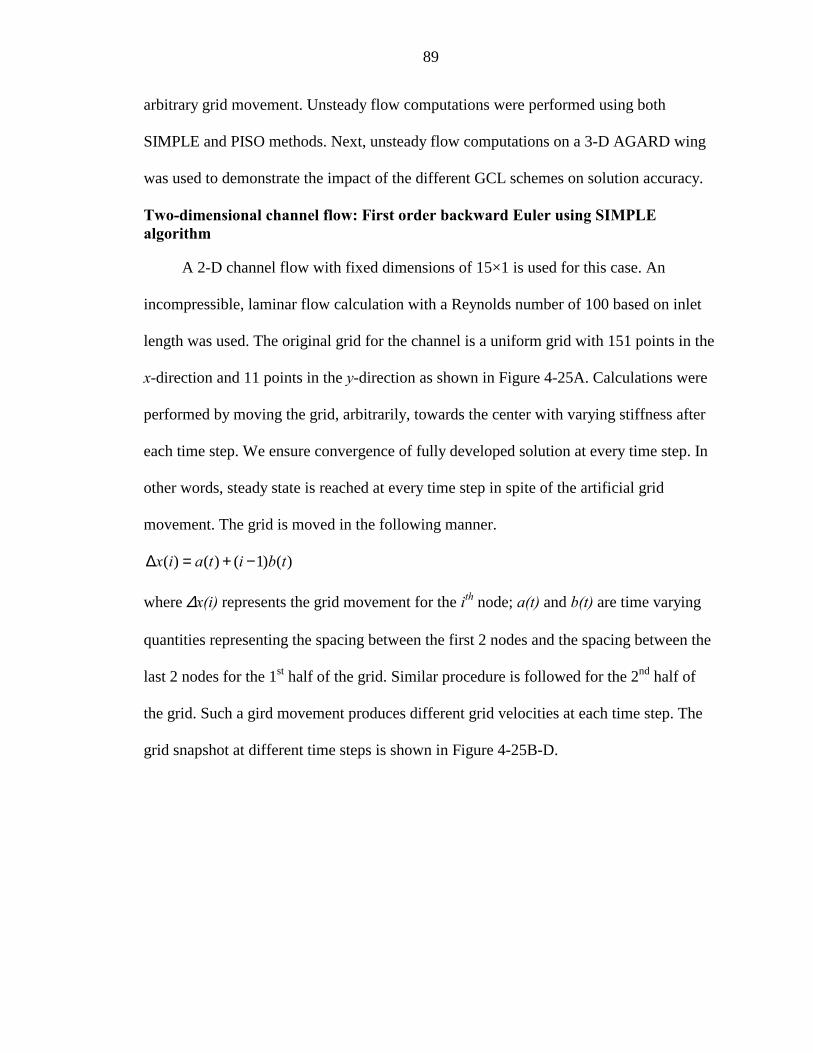
89
arbitrary grid movement. Unsteady flow computations were performed using both
SIMPLE and PISO methods. Next, unsteady flow computations on a 3-D AGARD wing
was used to demonstrate the impact of the different GCL schemes on solution accuracy.
Two-dimensional channel flow: First order backward Euler using SIMPLE algorithm
A 2-D channel flow with fixed dimensions of 15×1 is used for this case. An
incompressible, laminar flow calculation with a Reynolds number of 100 based on inlet
length was used. The original grid for the channel is a uniform grid with 151 points in the
x-direction and 11 points in the y-direction as shown in Figure 4-25A. Calculations were
performed by moving the grid, arbitrarily, towards the center with varying stiffness after
each time step. We ensure convergence of fully developed solution at every time step. In
other words, steady state is reached at every time step in spite of the artificial grid
movement. The grid is moved in the following manner.
( ) ( ) ( 1) ( )x i a t i b t∆ = + −
where ∆x(i) represents the grid movement for the ith node; a(t) and b(t) are time varying
quantities representing the spacing between the first 2 nodes and the spacing between the
last 2 nodes for the 1st half of the grid. Similar procedure is followed for the 2nd half of
the grid. Such a gird movement produces different grid velocities at each time step. The
grid snapshot at different time steps is shown in Figure 4-25B-D.
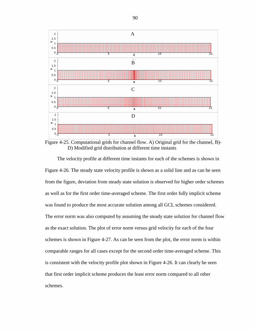
90
Figure 4-25. Computational grids for channel flow. A) Original grid for the channel, B)-D) Modified grid distribution at different time instants
The velocity profile at different time instants for each of the schemes is shown in
Figure 4-26. The steady state velocity profile is shown as a solid line and as can be seen
from the figure, deviation from steady state solution is observed for higher order schemes
as well as for the first order time-averaged scheme. The first order fully implicit scheme
was found to produce the most accurate solution among all GCL schemes considered.
The error norm was also computed by assuming the steady state solution for channel flow
as the exact solution. The plot of error norm versus grid velocity for each of the four
schemes is shown in Figure 4-27. As can be seen from the plot, the error norm is within
comparable ranges for all cases except for the second order time-averaged scheme. This
is consistent with the velocity profile plot shown in Figure 4-26. It can clearly be seen
that first order implicit scheme produces the least error norm compared to all other
schemes.
X
Y
0 5 10 150
0.5
1
1.5
2 (b)
X
Y
0 5 10 150
0.5
1
1.5
2 (d)
X
Y
0 5 10 150
0.51
1.5
2 (c)
XY
0 5 10 1500.5
1
1.52 (a)A
B
C
D
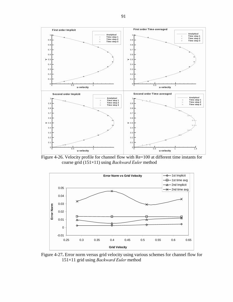
91
Figure 4-26. Velocity profile for channel flow with Re=100 at different time instants for coarse grid (151×11) using Backward Euler method
Figure 4-27. Error norm versus grid velocity using various schemes for channel flow for 151×11 grid using Backward Euler method
u-velocity
Y
0 0.5 10
0.1
0.2
0.3
0.4
0.5
0.6
0.7
0.8
0.9
1 Analytica lT ime step 1T ime step 2T ime step 3
F irst order T ime-averaged
u-velocity
Y
0 0.5 1 1.50
0.1
0.2
0.3
0.4
0.5
0.6
0.7
0.8
0.9
1 Analytica lT im e step 1T im e step 2T im e step 3
S econd order T ime-averaged
u-velocity
Y
0 0.5 10
0.1
0.2
0.3
0.4
0.5
0.6
0.7
0.8
0.9
1 Analytica lTim e step 1Tim e step 2Tim e step 3
S econd order Implciit
u-velocity
Y
0 0.5 10
0.1
0.2
0.3
0.4
0.5
0.6
0.7
0.8
0.9
1 Analytica lTim e step 1Tim e step 2Tim e step 3
F irst order Implicit
Error Norm vs Grid Velocity
-0.01
0
0.01
0.02
0.03
0.04
0.05
0.25 0.3 0.35 0.4 0.45 0.5 0.55 0.6 0.65
Grid Velocity
Erro
r Nor
m
1st Implicit1st time avg2nd Implicit2nd time avg

92
A grid refinement study was done on the same test case by doubling the number of
grid points in both directions. A similar grid movement pattern was used here. The plot of
velocity profiles is shown in Figure 4-28. The error norm versus grid velocity is shown in
Figure 4-29 and as can be seen from the figure, the pattern is very similar as compared to
the coarse grid case; however the magnitude of error is less for fine grid case than coarse
grid case as expected. Thus we can infer that there is not much of an advantage of using a
higher order GCL scheme as compared to a first order implicit scheme. This observation
can be understood with the view that GCL could be related to Guillard and Farhat’s
(2000) statement that for a p-order time-accurate scheme on a fixed mesh, satisfying the
p-order accurate DGCL is a sufficient condition for the scheme to be first order time
accurate on a moving mesh. The above statement coupled with the fact that our flow
solver is first order implicit in time leads to the observation that the first order GCL
scheme performs the best among the schemes considered.
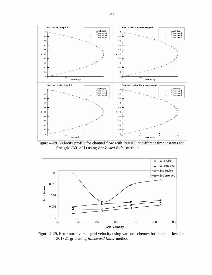
93
Figure 4-28. Velocity profile for channel flow with Re=100 at different time instants for fine grid (301×21) using Backward Euler method
Figure 4-29. Error norm versus grid velocity using various schemes for channel flow for 301×21 grid using Backward Euler method
0
0.005
0.01
0.015
0.02
0.3 0.4 0.5 0.6 0.7 0.8 0.9
Grid Velocity
Erro
r Nor
m
1st Implicit
1st time avg
2nd Implicit
2nd time avg
u-velocity
Y
0 0.5 10
0.1
0.2
0.3
0.4
0.5
0.6
0.7
0.8
0.9
1 Analytica lT ime step 1T ime step 2T ime step 3
F irst order Implicit
u-velocity
Y
0 0.5 10
0.1
0.2
0.3
0.4
0.5
0.6
0.7
0.8
0.9
1 Analytica lT ime step 1T ime step 2T ime step 3
F irst order T ime-averaged
u-velocity
Y
0 0.5 10
0.1
0.2
0.3
0.4
0.5
0.6
0.7
0.8
0.9
1 Analytica lT ime step 1T ime step 2T ime step 3
S econd order Implicit
u-velocity
Y
0 0.5 1 1.50
0.1
0.2
0.3
0.4
0.5
0.6
0.7
0.8
0.9
1 Analytica lT ime step 1T ime step 2T ime step 3
S econd order T ime-averaged
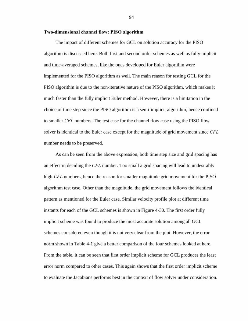
94
Two-dimensional channel flow: PISO algorithm
The impact of different schemes for GCL on solution accuracy for the PISO
algorithm is discussed here. Both first and second order schemes as well as fully implicit
and time-averaged schemes, like the ones developed for Euler algorithm were
implemented for the PISO algorithm as well. The main reason for testing GCL for the
PISO algorithm is due to the non-iterative nature of the PISO algorithm, which makes it
much faster than the fully implicit Euler method. However, there is a limitation in the
choice of time step since the PISO algorithm is a semi-implicit algorithm, hence confined
to smaller CFL numbers. The test case for the channel flow case using the PISO flow
solver is identical to the Euler case except for the magnitude of grid movement since CFL
number needs to be preserved.
As can be seen from the above expression, both time step size and grid spacing has
an effect in deciding the CFL number. Too small a grid spacing will lead to undesirably
high CFL numbers, hence the reason for smaller magnitude grid movement for the PISO
algorithm test case. Other than the magnitude, the grid movement follows the identical
pattern as mentioned for the Euler case. Similar velocity profile plot at different time
instants for each of the GCL schemes is shown in Figure 4-30. The first order fully
implicit scheme was found to produce the most accurate solution among all GCL
schemes considered even though it is not very clear from the plot. However, the error
norm shown in Table 4-1 give a better comparison of the four schemes looked at here.
From the table, it can be seen that first order implicit scheme for GCL produces the least
error norm compared to other cases. This again shows that the first order implicit scheme
to evaluate the Jacobians performs best in the context of flow solver under consideration.
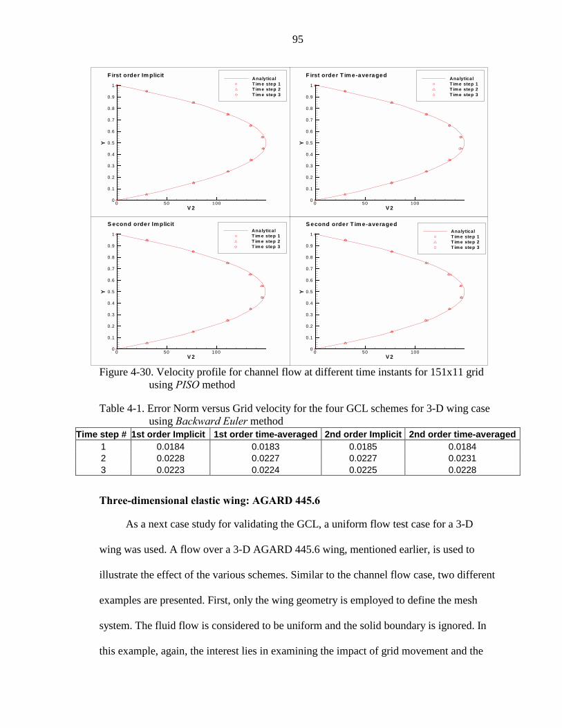
95
Figure 4-30. Velocity profile for channel flow at different time instants for 151x11 grid using PISO method
Table 4-1. Error Norm versus Grid velocity for the four GCL schemes for 3-D wing case using Backward Euler method
Time step # 1st order Implicit 1st order time-averaged 2nd order Implicit 2nd order time-averaged1 0.0184 0.0183 0.0185 0.0184 2 0.0228 0.0227 0.0227 0.0231 3 0.0223 0.0224 0.0225 0.0228
Three-dimensional elastic wing: AGARD 445.6
As a next case study for validating the GCL, a uniform flow test case for a 3-D
wing was used. A flow over a 3-D AGARD 445.6 wing, mentioned earlier, is used to
illustrate the effect of the various schemes. Similar to the channel flow case, two different
examples are presented. First, only the wing geometry is employed to define the mesh
system. The fluid flow is considered to be uniform and the solid boundary is ignored. In
this example, again, the interest lies in examining the impact of grid movement and the
V 2
Y
0 50 1000
0.1
0.2
0.3
0.4
0.5
0.6
0.7
0.8
0.9
1Ana lyticalT im e step 1T im e step 2T im e step 3
S econd order T im e-averaged
V 2
Y
0 50 1000
0.1
0.2
0.3
0.4
0.5
0.6
0.7
0.8
0.9
1Ana lyticalT im e step 1T im e step 2T im e step 3
F irst order T im e-averaged
V 2
Y
0 50 1000
0.1
0.2
0.3
0.4
0.5
0.6
0.7
0.8
0.9
1AnalyticalT im e step 1T im e step 2T im e step 3
F irst order Im plicit
V 2
Y
0 50 1000
0.1
0.2
0.3
0.4
0.5
0.6
0.7
0.8
0.9
1Ana lyticalT im e step 1T im e step 2T im e step 3
S econd order Im plicit
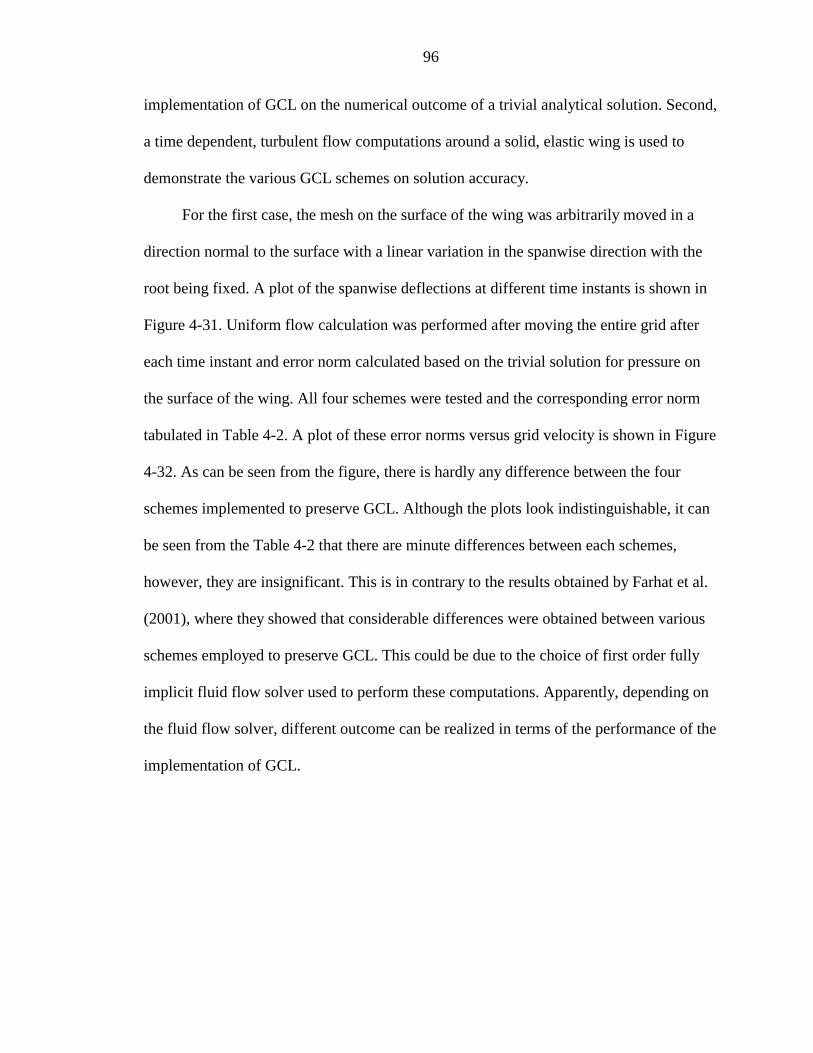
96
implementation of GCL on the numerical outcome of a trivial analytical solution. Second,
a time dependent, turbulent flow computations around a solid, elastic wing is used to
demonstrate the various GCL schemes on solution accuracy.
For the first case, the mesh on the surface of the wing was arbitrarily moved in a
direction normal to the surface with a linear variation in the spanwise direction with the
root being fixed. A plot of the spanwise deflections at different time instants is shown in
Figure 4-31. Uniform flow calculation was performed after moving the entire grid after
each time instant and error norm calculated based on the trivial solution for pressure on
the surface of the wing. All four schemes were tested and the corresponding error norm
tabulated in Table 4-2. A plot of these error norms versus grid velocity is shown in Figure
4-32. As can be seen from the figure, there is hardly any difference between the four
schemes implemented to preserve GCL. Although the plots look indistinguishable, it can
be seen from the Table 4-2 that there are minute differences between each schemes,
however, they are insignificant. This is in contrary to the results obtained by Farhat et al.
(2001), where they showed that considerable differences were obtained between various
schemes employed to preserve GCL. This could be due to the choice of first order fully
implicit fluid flow solver used to perform these computations. Apparently, depending on
the fluid flow solver, different outcome can be realized in terms of the performance of the
implementation of GCL.
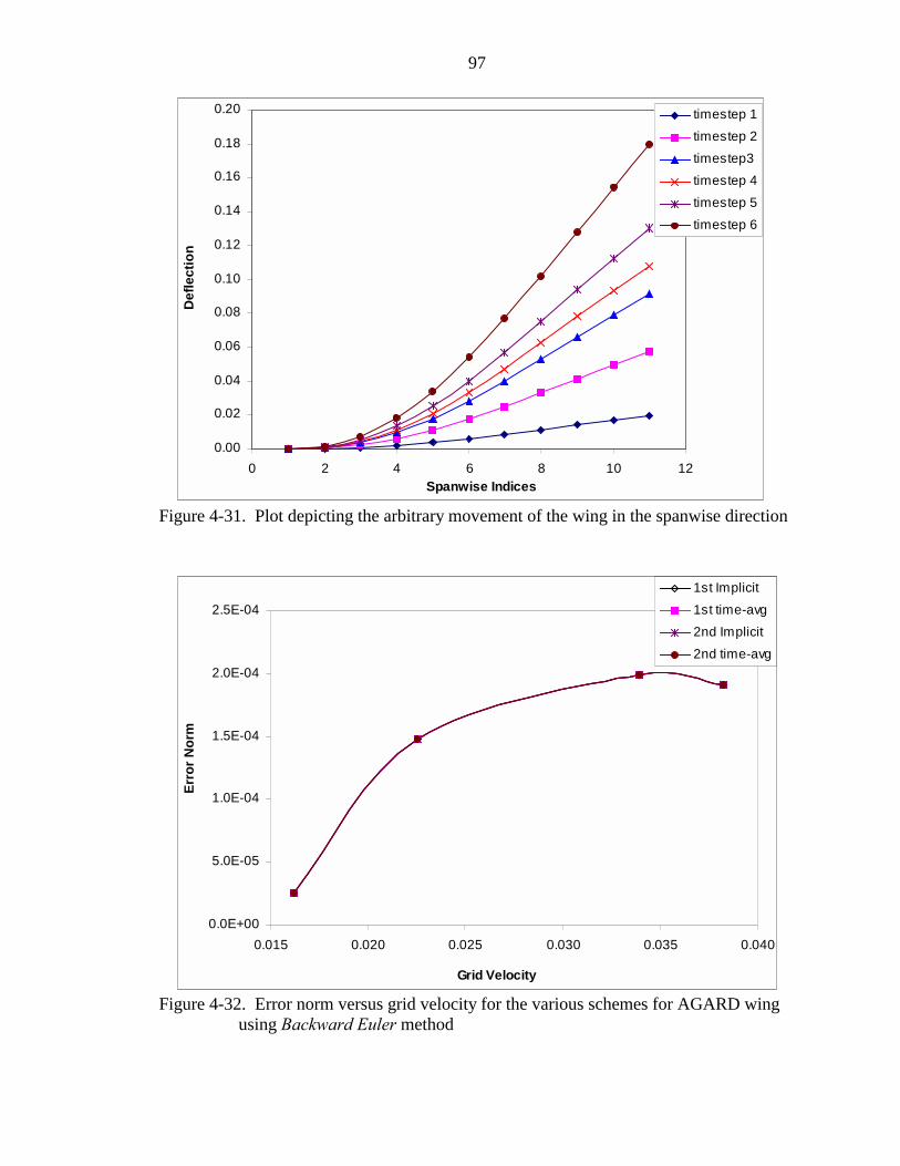
97
Figure 4-31. Plot depicting the arbitrary movement of the wing in the spanwise direction
Figure 4-32. Error norm versus grid velocity for the various schemes for AGARD wing using Backward Euler method
0.0E+00
5.0E-05
1.0E-04
1.5E-04
2.0E-04
2.5E-04
0.015 0.020 0.025 0.030 0.035 0.040
Grid Velocity
Erro
r Nor
m
1st Implicit
1st time-avg
2nd Implicit
2nd time-avg
0.00
0.02
0.04
0.06
0.08
0.10
0.12
0.14
0.16
0.18
0.20
0 2 4 6 8 10 12Spanwise Indices
Def
lect
ion
timestep 1
timestep 2
timestep3
timestep 4
timestep 5
timestep 6
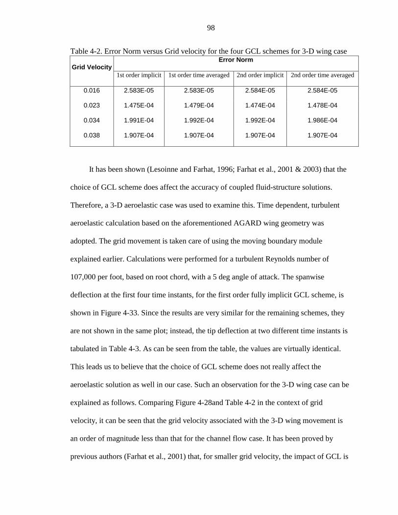
98
Table 4-2. Error Norm versus Grid velocity for the four GCL schemes for 3-D wing case Error Norm
Grid Velocity 1st order implicit 1st order time averaged 2nd order implicit 2nd order time averaged
0.016 2.583E-05 2.583E-05 2.584E-05 2.584E-05
0.023 1.475E-04 1.479E-04 1.474E-04 1.478E-04
0.034 1.991E-04 1.992E-04 1.992E-04 1.986E-04
0.038 1.907E-04 1.907E-04 1.907E-04 1.907E-04
It has been shown (Lesoinne and Farhat, 1996; Farhat et al., 2001 & 2003) that the
choice of GCL scheme does affect the accuracy of coupled fluid-structure solutions.
Therefore, a 3-D aeroelastic case was used to examine this. Time dependent, turbulent
aeroelastic calculation based on the aforementioned AGARD wing geometry was
adopted. The grid movement is taken care of using the moving boundary module
explained earlier. Calculations were performed for a turbulent Reynolds number of
107,000 per foot, based on root chord, with a 5 deg angle of attack. The spanwise
deflection at the first four time instants, for the first order fully implicit GCL scheme, is
shown in Figure 4-33. Since the results are very similar for the remaining schemes, they
are not shown in the same plot; instead, the tip deflection at two different time instants is
tabulated in Table 4-3. As can be seen from the table, the values are virtually identical.
This leads us to believe that the choice of GCL scheme does not really affect the
aeroelastic solution as well in our case. Such an observation for the 3-D wing case can be
explained as follows. Comparing Figure 4-28and Table 4-2 in the context of grid
velocity, it can be seen that the grid velocity associated with the 3-D wing movement is
an order of magnitude less than that for the channel flow case. It has been proved by
previous authors (Farhat et al., 2001) that, for smaller grid velocity, the impact of GCL is
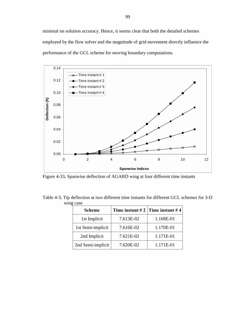
99
minimal on solution accuracy. Hence, it seems clear that both the detailed schemes
employed by the flow solver and the magnitude of grid movement directly influence the
performance of the GCL scheme for moving boundary computations.
Figure 4-33. Spanwise deflection of AGARD wing at four different time instants
Table 4-3. Tip deflection at two different time instants for different GCL schemes for 3-D wing case
Scheme Time instant # 2 Time instant # 4
1st Implicit 7.613E-02 1.168E-01
1st Semi-implicit 7.616E-02 1.170E-01
2nd Implicit 7.621E-02 1.171E-01
2nd Semi-implicit 7.620E-02 1.171E-01
0.00
0.02
0.04
0.06
0.08
0.10
0.12
0.14
0 2 4 6 8 10 12
Spanwise Indices
Def
lect
ion
(ft)
Time instant # 1
Time instant # 2
Time instant # 3
Time instant # 4
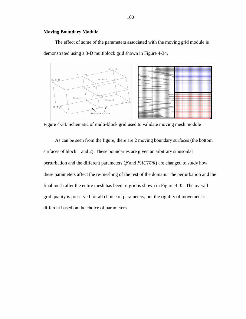
100
Moving Boundary Module
The effect of some of the parameters associated with the moving grid module is
demonstrated using a 3-D multiblock grid shown in Figure 4-34.
Figure 4-34. Schematic of multi-block grid used to validate moving mesh module
As can be seen from the figure, there are 2 moving boundary surfaces (the bottom
surfaces of block 1 and 2). These boundaries are given an arbitrary sinusoidal
perturbation and the different parameters (β and FACTOR) are changed to study how
these parameters affect the re-meshing of the rest of the domain. The perturbation and the
final mesh after the entire mesh has been re-grid is shown in Figure 4-35. The overall
grid quality is preserved for all choice of parameters, but the rigidity of movement is
different based on the choice of parameters.
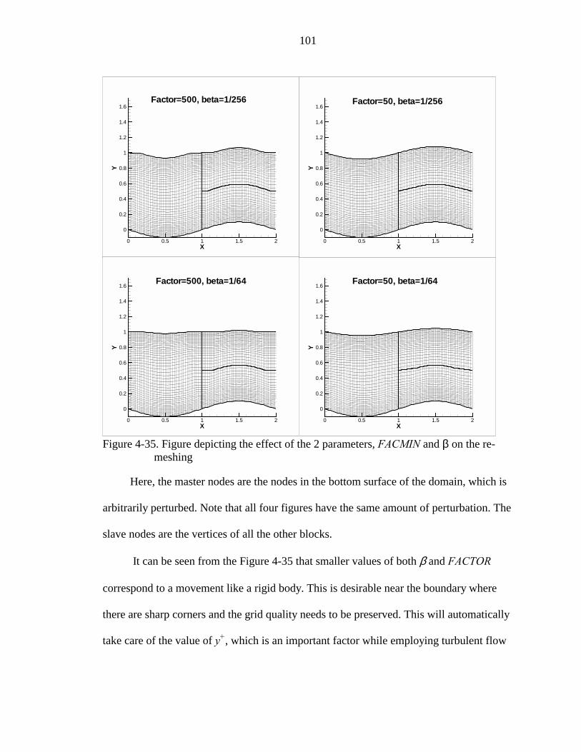
101
Figure 4-35. Figure depicting the effect of the 2 parameters, FACMIN and β on the re-meshing
Here, the master nodes are the nodes in the bottom surface of the domain, which is
arbitrarily perturbed. Note that all four figures have the same amount of perturbation. The
slave nodes are the vertices of all the other blocks.
It can be seen from the Figure 4-35 that smaller values of both β and FACTOR
correspond to a movement like a rigid body. This is desirable near the boundary where
there are sharp corners and the grid quality needs to be preserved. This will automatically
take care of the value of y+, which is an important factor while employing turbulent flow
X
Y
0 0.5 1 1.5 2
0
0.2
0.4
0.6
0.8
1
1.2
1.4
1.6Factor=500, beta=1/256
X
Y
0 0.5 1 1.5 2
0
0.2
0.4
0.6
0.8
1
1.2
1.4
1.6Factor=50, beta=1/64
X
Y
0 0.5 1 1.5 2
0
0.2
0.4
0.6
0.8
1
1.2
1.4
1.6Factor=500, beta=1/64
X
Y
0 0.5 1 1.5 2
0
0.2
0.4
0.6
0.8
1
1.2
1.4
1.6Factor=50, beta=1/256
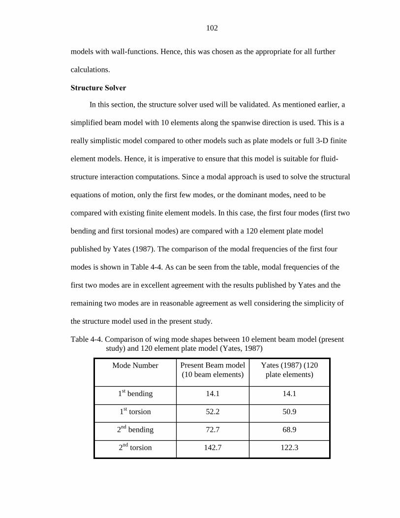
102
models with wall-functions. Hence, this was chosen as the appropriate for all further
calculations.
Structure Solver
In this section, the structure solver used will be validated. As mentioned earlier, a
simplified beam model with 10 elements along the spanwise direction is used. This is a
really simplistic model compared to other models such as plate models or full 3-D finite
element models. Hence, it is imperative to ensure that this model is suitable for fluid-
structure interaction computations. Since a modal approach is used to solve the structural
equations of motion, only the first few modes, or the dominant modes, need to be
compared with existing finite element models. In this case, the first four modes (first two
bending and first torsional modes) are compared with a 120 element plate model
published by Yates (1987). The comparison of the modal frequencies of the first four
modes is shown in Table 4-4. As can be seen from the table, modal frequencies of the
first two modes are in excellent agreement with the results published by Yates and the
remaining two modes are in reasonable agreement as well considering the simplicity of
the structure model used in the present study.
Table 4-4. Comparison of wing mode shapes between 10 element beam model (present study) and 120 element plate model (Yates, 1987)
68.9 72.7 2nd bending
122.3 142.7 2nd torsion
50.9 52.2 1st torsion
14.1 14.1 1st bending
Yates (1987) (120 plate elements)
Present Beam model (10 beam elements)
Mode Number
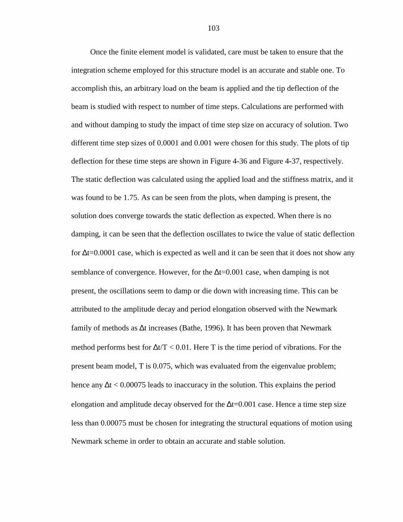
103
Once the finite element model is validated, care must be taken to ensure that the
integration scheme employed for this structure model is an accurate and stable one. To
accomplish this, an arbitrary load on the beam is applied and the tip deflection of the
beam is studied with respect to number of time steps. Calculations are performed with
and without damping to study the impact of time step size on accuracy of solution. Two
different time step sizes of 0.0001 and 0.001 were chosen for this study. The plots of tip
deflection for these time steps are shown in Figure 4-36 and Figure 4-37, respectively.
The static deflection was calculated using the applied load and the stiffness matrix, and it
was found to be 1.75. As can be seen from the plots, when damping is present, the
solution does converge towards the static deflection as expected. When there is no
damping, it can be seen that the deflection oscillates to twice the value of static deflection
for ∆t=0.0001 case, which is expected as well and it can be seen that it does not show any
semblance of convergence. However, for the ∆t=0.001 case, when damping is not
present, the oscillations seem to damp or die down with increasing time. This can be
attributed to the amplitude decay and period elongation observed with the Newmark
family of methods as ∆t increases (Bathe, 1996). It has been proven that Newmark
method performs best for ∆t/T < 0.01. Here T is the time period of vibrations. For the
present beam model, T is 0.075, which was evaluated from the eigenvalue problem;
hence any ∆t < 0.00075 leads to inaccuracy in the solution. This explains the period
elongation and amplitude decay observed for the ∆t=0.001 case. Hence a time step size
less than 0.00075 must be chosen for integrating the structural equations of motion using
Newmark scheme in order to obtain an accurate and stable solution.
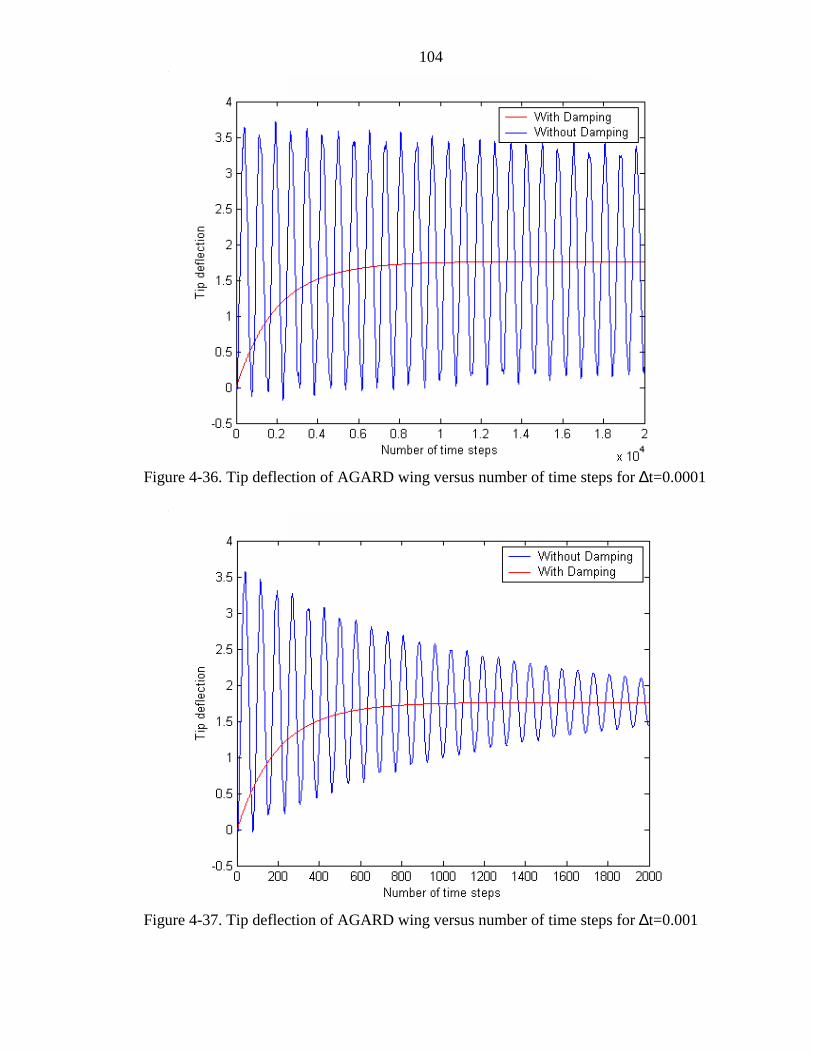
104
Figure 4-36. Tip deflection of AGARD wing versus number of time steps for ∆t=0.0001
Figure 4-37. Tip deflection of AGARD wing versus number of time steps for ∆t=0.001
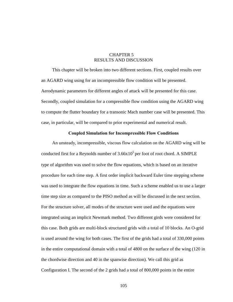
105
CHAPTER 5 RESULTS AND DISCUSSION
This chapter will be broken into two different sections. First, coupled results over
an AGARD wing using for an incompressible flow condition will be presented.
Aerodynamic parameters for different angles of attack will be presented for this case.
Secondly, coupled simulation for a compressible flow condition using the AGARD wing
to compute the flutter boundary for a transonic Mach number case will be presented. This
case, in particular, will be compared to prior experimental and numerical result.
Coupled Simulation for Incompressible Flow Conditions
An unsteady, incompressible, viscous flow calculation on the AGARD wing will be
conducted first for a Reynolds number of 3.66x10⁵ per foot of root chord. A SIMPLE
type of algorithm was used to solve the flow equations, which is based on an iterative
procedure for each time step. A first order implicit backward Euler time stepping scheme
was used to integrate the flow equations in time. Such a scheme enabled us to use a larger
time step size as compared to the PISO method as will be discussed in the next section.
For the structure solver, all modes of the structure were used and the equations were
integrated using an implicit Newmark method. Two different girds were considered for
this case. Both grids are multi-block structured grids with a total of 10 blocks. An O-grid
is used around the wing for both cases. The first of the grids had a total of 330,000 points
in the entire computational domain with a total of 4800 on the surface of the wing (120 in
the chordwise direction and 40 in the spanwise direction). We call this grid as
Configuration I. The second of the 2 grids had a total of 800,000 points in the entire
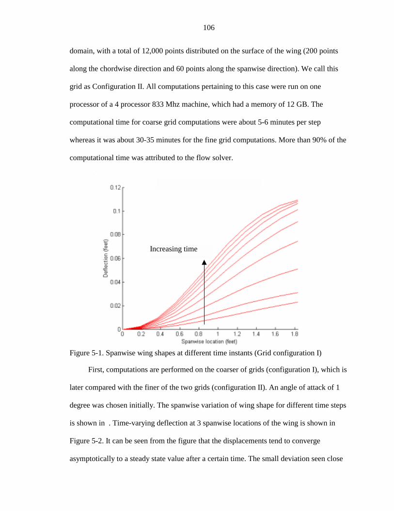
106
domain, with a total of 12,000 points distributed on the surface of the wing (200 points
along the chordwise direction and 60 points along the spanwise direction). We call this
grid as Configuration II. All computations pertaining to this case were run on one
processor of a 4 processor 833 Mhz machine, which had a memory of 12 GB. The
computational time for coarse grid computations were about 5-6 minutes per step
whereas it was about 30-35 minutes for the fine grid computations. More than 90% of the
computational time was attributed to the flow solver.
Figure 5-1. Spanwise wing shapes at different time instants (Grid configuration I)
First, computations are performed on the coarser of grids (configuration I), which is
later compared with the finer of the two grids (configuration II). An angle of attack of 1
degree was chosen initially. The spanwise variation of wing shape for different time steps
is shown in . Time-varying deflection at 3 spanwise locations of the wing is shown in
Figure 5-2. It can be seen from the figure that the displacements tend to converge
asymptotically to a steady state value after a certain time. The small deviation seen close
Increasing time
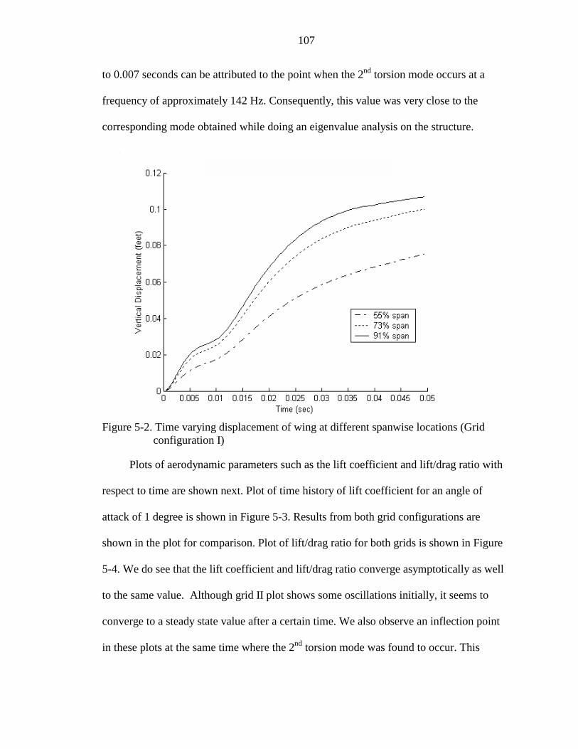
107
to 0.007 seconds can be attributed to the point when the 2nd torsion mode occurs at a
frequency of approximately 142 Hz. Consequently, this value was very close to the
corresponding mode obtained while doing an eigenvalue analysis on the structure.
Figure 5-2. Time varying displacement of wing at different spanwise locations (Grid configuration I)
Plots of aerodynamic parameters such as the lift coefficient and lift/drag ratio with
respect to time are shown next. Plot of time history of lift coefficient for an angle of
attack of 1 degree is shown in Figure 5-3. Results from both grid configurations are
shown in the plot for comparison. Plot of lift/drag ratio for both grids is shown in Figure
5-4. We do see that the lift coefficient and lift/drag ratio converge asymptotically as well
to the same value. Although grid II plot shows some oscillations initially, it seems to
converge to a steady state value after a certain time. We also observe an inflection point
in these plots at the same time where the 2nd torsion mode was found to occur. This
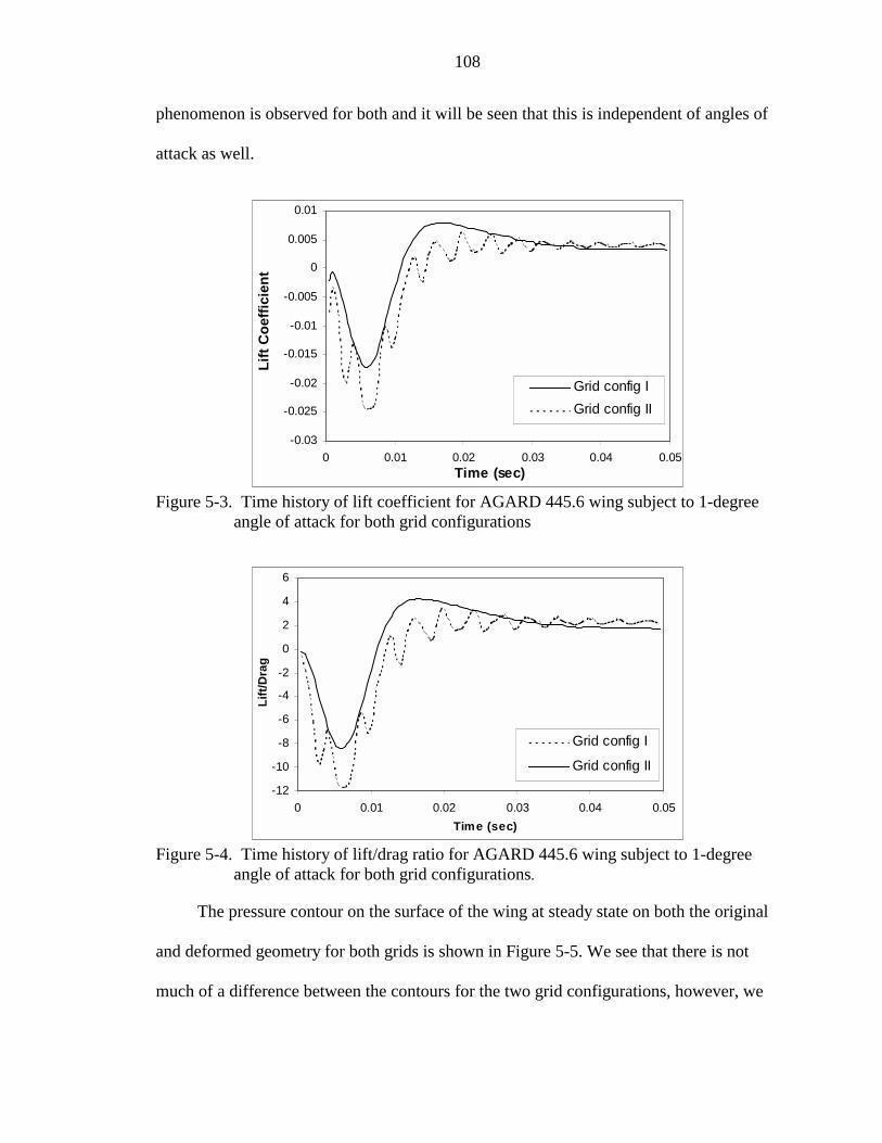
108
phenomenon is observed for both and it will be seen that this is independent of angles of
attack as well.
Figure 5-3. Time history of lift coefficient for AGARD 445.6 wing subject to 1-degree angle of attack for both grid configurations
Figure 5-4. Time history of lift/drag ratio for AGARD 445.6 wing subject to 1-degree angle of attack for both grid configurations.
The pressure contour on the surface of the wing at steady state on both the original
and deformed geometry for both grids is shown in Figure 5-5. We see that there is not
much of a difference between the contours for the two grid configurations, however, we
-0.03
-0.025
-0.02
-0.015
-0.01
-0.005
0
0.005
0.01
0 0.01 0.02 0.03 0.04 0.05Time (sec)
Lift
Coe
ffici
ent
Grid config IGrid config II
-12
-10
-8
-6
-4
-2
0
2
4
6
0 0.01 0.02 0.03 0.04 0.05Time (sec)
Lift/
Dra
g
Grid config I
Grid config II
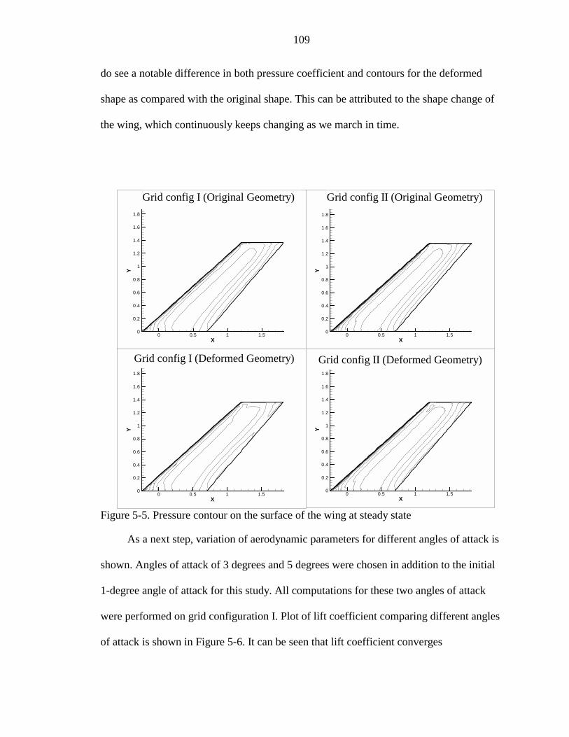
109
do see a notable difference in both pressure coefficient and contours for the deformed
shape as compared with the original shape. This can be attributed to the shape change of
the wing, which continuously keeps changing as we march in time.
Figure 5-5. Pressure contour on the surface of the wing at steady state
As a next step, variation of aerodynamic parameters for different angles of attack is
shown. Angles of attack of 3 degrees and 5 degrees were chosen in addition to the initial
1-degree angle of attack for this study. All computations for these two angles of attack
were performed on grid configuration I. Plot of lift coefficient comparing different angles
of attack is shown in Figure 5-6. It can be seen that lift coefficient converges
X
Y
0 0.5 1 1.50
0.2
0.4
0.6
0.8
1
1.2
1.4
1.6
1.8
Coarse grid (Deformed Geometry)
X
Y
0 0.5 1 1.50
0.2
0.4
0.6
0.8
1
1.2
1.4
1.6
1.8
Fine grid (Deformed Geometry)
X
Y
0 0.5 1 1.50
0.2
0.4
0.6
0.8
1
1.2
1.4
1.6
1.8
Fine grid (Original Geometry)
X
Y
0 0.5 1 1.50
0.2
0.4
0.6
0.8
1
1.2
1.4
1.6
1.8
Coarse grid (Original Geometry)Grid config I (Original Geometry) Grid config II (Original Geometry)
Grid config I (Deformed Geometry) Grid config II (Deformed Geometry)
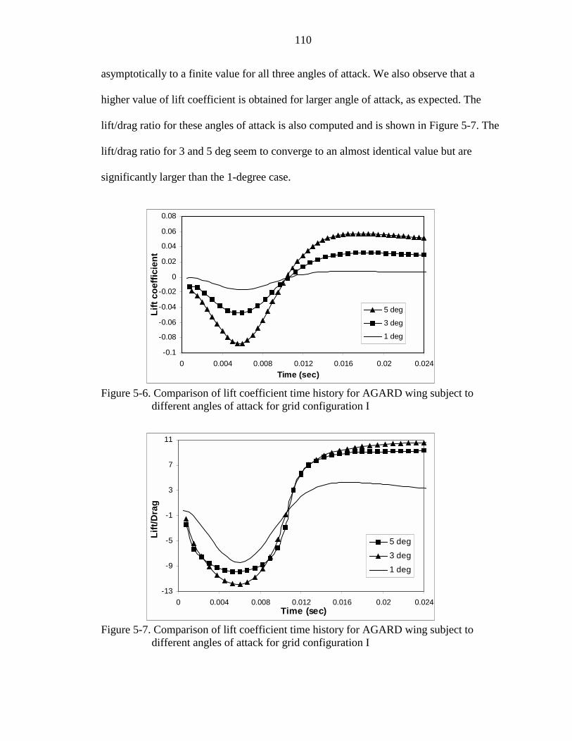
110
asymptotically to a finite value for all three angles of attack. We also observe that a
higher value of lift coefficient is obtained for larger angle of attack, as expected. The
lift/drag ratio for these angles of attack is also computed and is shown in Figure 5-7. The
lift/drag ratio for 3 and 5 deg seem to converge to an almost identical value but are
significantly larger than the 1-degree case.
Figure 5-6. Comparison of lift coefficient time history for AGARD wing subject to different angles of attack for grid configuration I
Figure 5-7. Comparison of lift coefficient time history for AGARD wing subject to different angles of attack for grid configuration I
-0.1
-0.08
-0.06
-0.04
-0.02
0
0.02
0.04
0.06
0.08
0 0.004 0.008 0.012 0.016 0.02 0.024Time (sec)
Lift
coef
ficie
nt
5 deg
3 deg
1 deg
-13
-9
-5
-1
3
7
11
0 0.004 0.008 0.012 0.016 0.02 0.024Time (sec)
Lift/
Dra
g
5 deg
3 deg
1 deg

111
Comparison of PISO and SIMPLE Algorithms
Since the flow solver consumes most of the CPU time during a coupled simulation,
a non-iterative method based on PISO algorithm was proposed to perform flow
computations instead of the SIMPLE algorithm, which was an iterative method as
mentioned before. As a first step towards developing this capability for fluid-structure
interaction computations, the PISO algorithm was compared with the SIMPLE algorithm
to ensure similar results between the two schemes when identical time step size is used
and to also compare the computational cost between the solvers. Coupled simulations
were carried out using the above-mentioned example for a Reynolds number of 3.64x10⁵
based on unit chord length. Grid configuration I is used for these computations. A plot
comparing the spanwise wing displacement at three consecutive time instants is shown in
Figure 5-8. As can be seen from the figure, the agreement is very good between these two
algorithms. The computational cost, however, by using the PISO algorithm was greatly
reduced compared to the SIMPLE algorithm. The ratio of the CPU time requirement
between the SIMPLE and PISO approach is about 10 per time step for this grid. Even
though the implicit nature of SIMPLE algorithm allows us to choose a larger time step
and still produce a stable solution, we still need to choose a small time step to obtain
good accuracy as the time marching scheme is first order in nature. Also, the frequencies
pertaining to the structure limits the choice of a higher time step size.
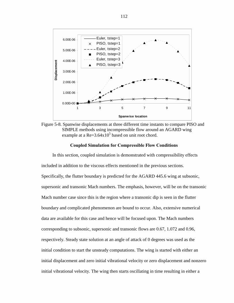
112
Figure 5-8. Spanwise displacements at three different time instants to compare PISO and SIMPLE methods using incompressible flow around an AGARD wing example at a Re=3.64x10⁵ based on unit root chord.
Coupled Simulation for Compressible Flow Conditions
In this section, coupled simulation is demonstrated with compressibility effects
included in addition to the viscous effects mentioned in the previous sections.
Specifically, the flutter boundary is predicted for the AGARD 445.6 wing at subsonic,
supersonic and transonic Mach numbers. The emphasis, however, will be on the transonic
Mach number case since this is the region where a transonic dip is seen in the flutter
boundary and complicated phenomenon are bound to occur. Also, extensive numerical
data are available for this case and hence will be focused upon. The Mach numbers
corresponding to subsonic, supersonic and transonic flows are 0.67, 1.072 and 0.96,
respectively. Steady state solution at an angle of attack of 0 degrees was used as the
initial condition to start the unsteady computations. The wing is started with either an
initial displacement and zero initial vibrational velocity or zero displacement and nonzero
initial vibrational velocity. The wing then starts oscillating in time resulting in either a
0.00E+00
1.00E-06
2.00E-06
3.00E-06
4.00E-06
5.00E-06
6.00E-06
1 3 5 7 9 11
Spanwise location
Dis
plac
emen
t
Euler, tstep=1PISO, tstep=1Euler, tstep=2PISO, tstep=2Euler, tstep=3PISO, tstep=3
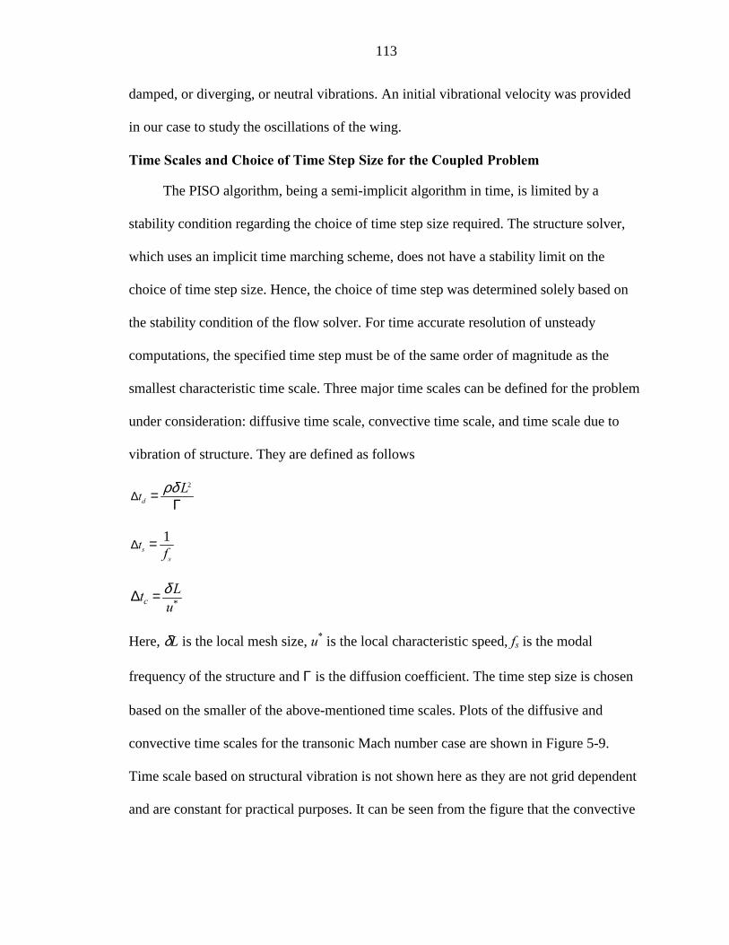
113
damped, or diverging, or neutral vibrations. An initial vibrational velocity was provided
in our case to study the oscillations of the wing.
Time Scales and Choice of Time Step Size for the Coupled Problem
The PISO algorithm, being a semi-implicit algorithm in time, is limited by a
stability condition regarding the choice of time step size required. The structure solver,
which uses an implicit time marching scheme, does not have a stability limit on the
choice of time step size. Hence, the choice of time step was determined solely based on
the stability condition of the flow solver. For time accurate resolution of unsteady
computations, the specified time step must be of the same order of magnitude as the
smallest characteristic time scale. Three major time scales can be defined for the problem
under consideration: diffusive time scale, convective time scale, and time scale due to
vibration of structure. They are defined as follows
2
dtLρδ
∆ =Γ
1s
s
t f∆ =
*cLt
uδ∆ =
Here, δL is the local mesh size, u* is the local characteristic speed, fs is the modal
frequency of the structure and Γ is the diffusion coefficient. The time step size is chosen
based on the smaller of the above-mentioned time scales. Plots of the diffusive and
convective time scales for the transonic Mach number case are shown in Figure 5-9.
Time scale based on structural vibration is not shown here as they are not grid dependent
and are constant for practical purposes. It can be seen from the figure that the convective
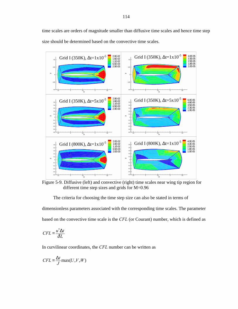
114
time scales are orders of magnitude smaller than diffusive time scales and hence time step
size should be determined based on the convective time scales.
Figure 5-9. Diffusive (left) and convective (right) time scales near wing tip region for different time step sizes and grids for M=0.96
The criteria for choosing the time step size can also be stated in terms of
dimensionless parameters associated with the corresponding time scales. The parameter
based on the convective time scale is the CFL (or Courant) number, which is defined as
*u tCFL L∆= δ
In curvilinear coordinates, the CFL number can be written as
max( , , )tCFL U V WJ∆=
X
Z
1.5 2 2.5 3 3.5-0.5
-0.25
0
0.25
0.5
2.0E-021.6E-021.1E-026.5E-032.0E-03
X
Z
1.5 2 2.5 3 3.5-0.5
-0.25
0
0.25
0.5
4.0E-053.3E-052.5E-051.8E-051.0E-05
X
Z
1.5 2 2.5 3 3.5-0.5
-0.4
-0.3
-0.2
-0.1
0
0.1
0.2
0.3
0.4
0.56.0E-054.8E-053.5E-052.3E-051.0E-05
X
Z
1.5 2 2.5 3 3.5-0.5
-0.4
-0.3
-0.2
-0.1
0
0.1
0.2
0.3
0.4
0.5
4.0E-053.3E-052.5E-051.8E-051.0E-05
X
Z
1.5 2 2.5 3 3.5-0.5
-0.4
-0.3
-0.2
-0.1
0
0.1
0.2
0.3
0.4
0.5
2.0E-021.6E-021.1E-026.5E-032.0E-03
X
Z
1.5 2 2.5 3 3.5-0.5
-0.4
-0.3
-0.2
-0.1
0
0.1
0.2
0.3
0.4
0.5
2.0E-021.6E-021.1E-026.5E-032.0E-03
Grid I (350K), ∆t=1x10⁻⁵ Grid I (350K), ∆t=1x10⁻⁵
Grid I (350K), ∆t=5x10⁻⁵ Grid I (350K), ∆t=5x10⁻⁵
Grid I (800K), ∆t=1x10⁻⁵ Grid I (800K), ∆t=1x10⁻⁵
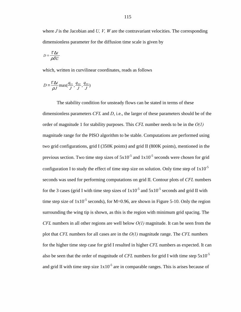
115
where J is the Jacobian and U, V, W are the contravariant velocities. The corresponding
dimensionless parameter for the diffusion time scale is given by
2D
tLρδ
=Γ∆
which, written in curvilinear coordinates, reads as follows
The stability condition for unsteady flows can be stated in terms of these
dimensionless parameters CFL and D, i.e., the larger of these parameters should be of the
order of magnitude 1 for stability purposes. This CFL number needs to be in the O(1)
magnitude range for the PISO algorithm to be stable. Computations are performed using
two grid configurations, grid I (350K points) and grid II (800K points), mentioned in the
previous section. Two time step sizes of 5x10⁻⁵ and 1x10⁻⁵ seconds were chosen for grid
configuration I to study the effect of time step size on solution. Only time step of 1x10⁻⁵
seconds was used for performing computations on grid II. Contour plots of CFL numbers
for the 3 cases (grid I with time step sizes of 1x10⁻⁵ and 5x10⁻⁵ seconds and grid II with
time step size of 1x10⁻⁵ seconds), for M=0.96, are shown in Figure 5-10. Only the region
surrounding the wing tip is shown, as this is the region with minimum grid spacing. The
CFL numbers in all other regions are well below O(1) magnitude. It can be seen from the
plot that CFL numbers for all cases are in the O(1) magnitude range. The CFL numbers
for the higher time step case for grid I resulted in higher CFL numbers as expected. It can
also be seen that the order of magnitude of CFL numbers for grid I with time step 5x10⁻⁵
and grid II with time step size 1x10⁻⁵ are in comparable ranges. This is arises because of
3311 22max( , , )qq qtDJ J J Jρ
Γ∆=
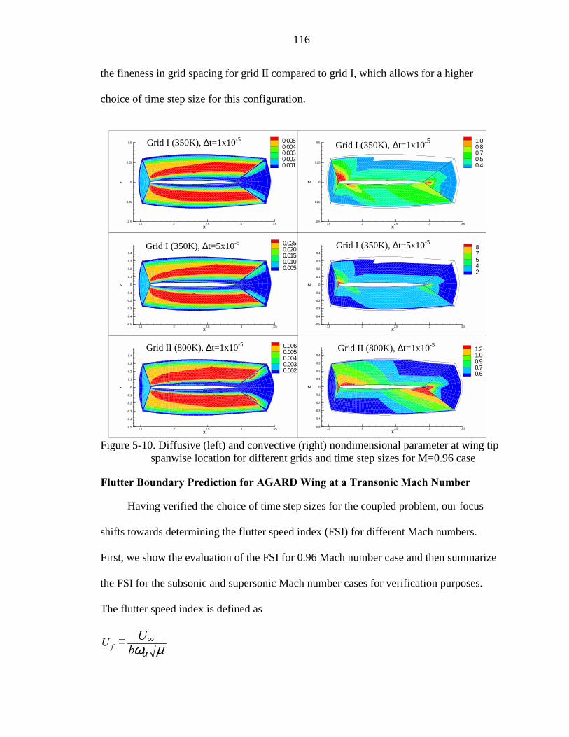
116
the fineness in grid spacing for grid II compared to grid I, which allows for a higher
choice of time step size for this configuration.
Figure 5-10. Diffusive (left) and convective (right) nondimensional parameter at wing tip spanwise location for different grids and time step sizes for M=0.96 case
Flutter Boundary Prediction for AGARD Wing at a Transonic Mach Number
Having verified the choice of time step sizes for the coupled problem, our focus
shifts towards determining the flutter speed index (FSI) for different Mach numbers.
First, we show the evaluation of the FSI for 0.96 Mach number case and then summarize
the FSI for the subsonic and supersonic Mach number cases for verification purposes.
The flutter speed index is defined as
fU Ub
∞=αω µ
X
Z
1.5 2 2.5 3 3.5-0.5
-0.25
0
0.25
0.5 1.00.80.70.50.4
X
Z
1.5 2 2.5 3 3.5-0.5
-0.4
-0.3
-0.2
-0.1
0
0.1
0.2
0.3
0.487542
X
Z
1.5 2 2.5 3 3.5-0.5
-0.4
-0.3
-0.2
-0.1
0
0.1
0.2
0.3
0.4
1.21.00.90.70.6
X
Z
1.5 2 2.5 3 3.5-0.5
-0.4
-0.3
-0.2
-0.1
0
0.1
0.2
0.3
0.4
0.0060.0050.0040.0030.002
X
Z
1.5 2 2.5 3 3.5-0.5
-0.25
0
0.25
0.5 0.0050.0040.0030.0020.001
X
Z
1.5 2 2.5 3 3.5-0.5
-0.4
-0.3
-0.2
-0.1
0
0.1
0.2
0.3
0.4
0.0250.0200.0150.0100.005
Grid I (350K), ∆t=1x10⁻⁵Grid I (350K), ∆t=1x10⁻⁵
Grid I (350K), ∆t=5x10⁻⁵
Grid II (800K), ∆t=1x10⁻⁵ Grid II (800K), ∆t=1x10⁻⁵
Grid I (350K), ∆t=5x10⁻⁵
117
where U∞ is the freestream velocity, b is the half root chord, ωα is the first torsional mode
frequency and µ is the mass ratio of the wing. It represents the condition at which the
oscillation is neither growing nor decaying. If the speed index U is smaller than Uf, the
motion is stable and if U is greater than Uf, then the motion is unstable. Unsteady
computations were run for a series of dynamic pressures to determine the flutter point.
The freestream density and Mach number are held constant as the dynamic pressure is
varied to determine the flutter point, thereby leading to a variation in Reynolds number
and temperature in order to provide a consistent set of flow conditions. The Reynolds
number was in the range 5.96x10⁵ to 6.72x10⁵ for this particular Mach number for the
various dynamic pressures considered. This change in Reynolds number did not produce
a significant effect on the flow solutions.
The growth and decay of the second mode of the structure is studied to arrive at the
flutter point. The flutter point was obtained by running a solution for a significantly long
period of time to arrive at a neutrally stable solution, where the amplitude of oscillations
of the generalized displacement of the structure is neither growing nor decaying.
As a first step, we show computations performed using the grid configuration I
(350 K points). The generalized displacements for three different choices of dynamic
pressure ratios (1.03, 0.98 and 0.905) using a time step size of 5x10⁻⁵ seconds are shown
in Figure 5-11. The dynamic pressure ratio is measured with respect to the experimental
dynamic pressure at which neutrally stable flutter was predicted, which occurs at a value
of 2935 N/m2 (61.3 lbf/ft2) for a Mach number of 0.96. It can be seen from the plot that
the amplitude ratio decreases with decrease in dynamic pressure. Amplitude growth is
seen for two of the dynamic pressure ratios (1.03 and 0.98) whereas amplitude decay is
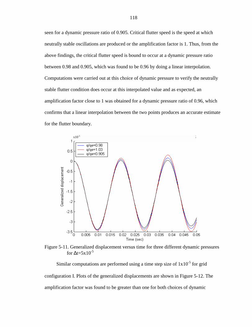
118
seen for a dynamic pressure ratio of 0.905. Critical flutter speed is the speed at which
neutrally stable oscillations are produced or the amplification factor is 1. Thus, from the
above findings, the critical flutter speed is bound to occur at a dynamic pressure ratio
between 0.98 and 0.905, which was found to be 0.96 by doing a linear interpolation.
Computations were carried out at this choice of dynamic pressure to verify the neutrally
stable flutter condition does occur at this interpolated value and as expected, an
amplification factor close to 1 was obtained for a dynamic pressure ratio of 0.96, which
confirms that a linear interpolation between the two points produces an accurate estimate
for the flutter boundary.
Figure 5-11. Generalized displacement versus time for three different dynamic pressures for ∆t=5x10⁻⁵
Similar computations are performed using a time step size of 1x10⁻⁵ for grid
configuration I. Plots of the generalized displacements are shown in Figure 5-12. The
amplification factor was found to be greater than one for both choices of dynamic
x10-5
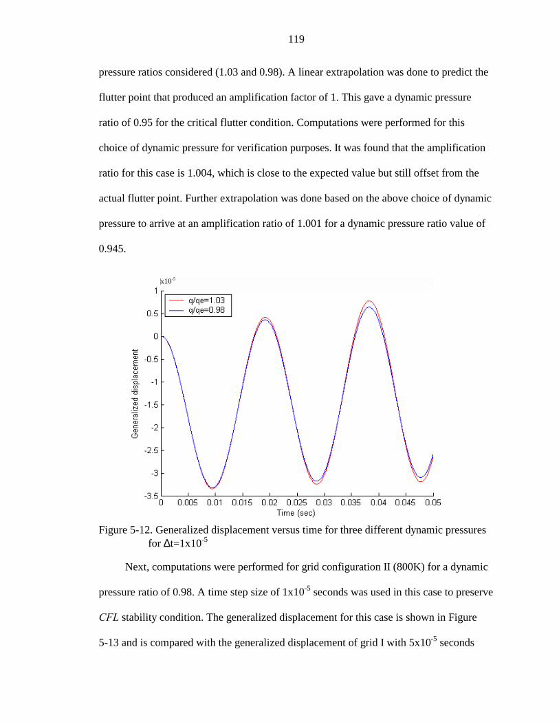
119
pressure ratios considered (1.03 and 0.98). A linear extrapolation was done to predict the
flutter point that produced an amplification factor of 1. This gave a dynamic pressure
ratio of 0.95 for the critical flutter condition. Computations were performed for this
choice of dynamic pressure for verification purposes. It was found that the amplification
ratio for this case is 1.004, which is close to the expected value but still offset from the
actual flutter point. Further extrapolation was done based on the above choice of dynamic
pressure to arrive at an amplification ratio of 1.001 for a dynamic pressure ratio value of
0.945.
Figure 5-12. Generalized displacement versus time for three different dynamic pressures for ∆t=1x10⁻⁵
Next, computations were performed for grid configuration II (800K) for a dynamic
pressure ratio of 0.98. A time step size of 1x10⁻⁵ seconds was used in this case to preserve
CFL stability condition. The generalized displacement for this case is shown in Figure
5-13 and is compared with the generalized displacement of grid I with 5x10⁻⁵ seconds
x10-5
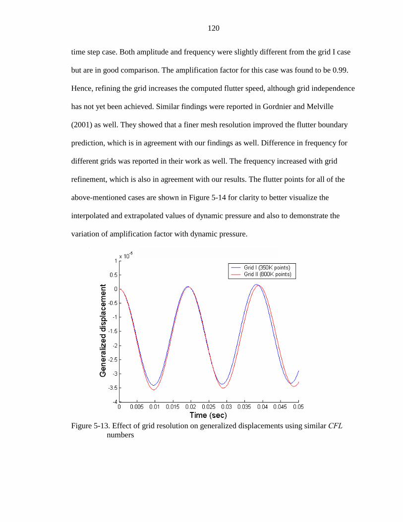
120
time step case. Both amplitude and frequency were slightly different from the grid I case
but are in good comparison. The amplification factor for this case was found to be 0.99.
Hence, refining the grid increases the computed flutter speed, although grid independence
has not yet been achieved. Similar findings were reported in Gordnier and Melville
(2001) as well. They showed that a finer mesh resolution improved the flutter boundary
prediction, which is in agreement with our findings as well. Difference in frequency for
different grids was reported in their work as well. The frequency increased with grid
refinement, which is also in agreement with our results. The flutter points for all of the
above-mentioned cases are shown in Figure 5-14 for clarity to better visualize the
interpolated and extrapolated values of dynamic pressure and also to demonstrate the
variation of amplification factor with dynamic pressure.
Figure 5-13. Effect of grid resolution on generalized displacements using similar CFL numbers
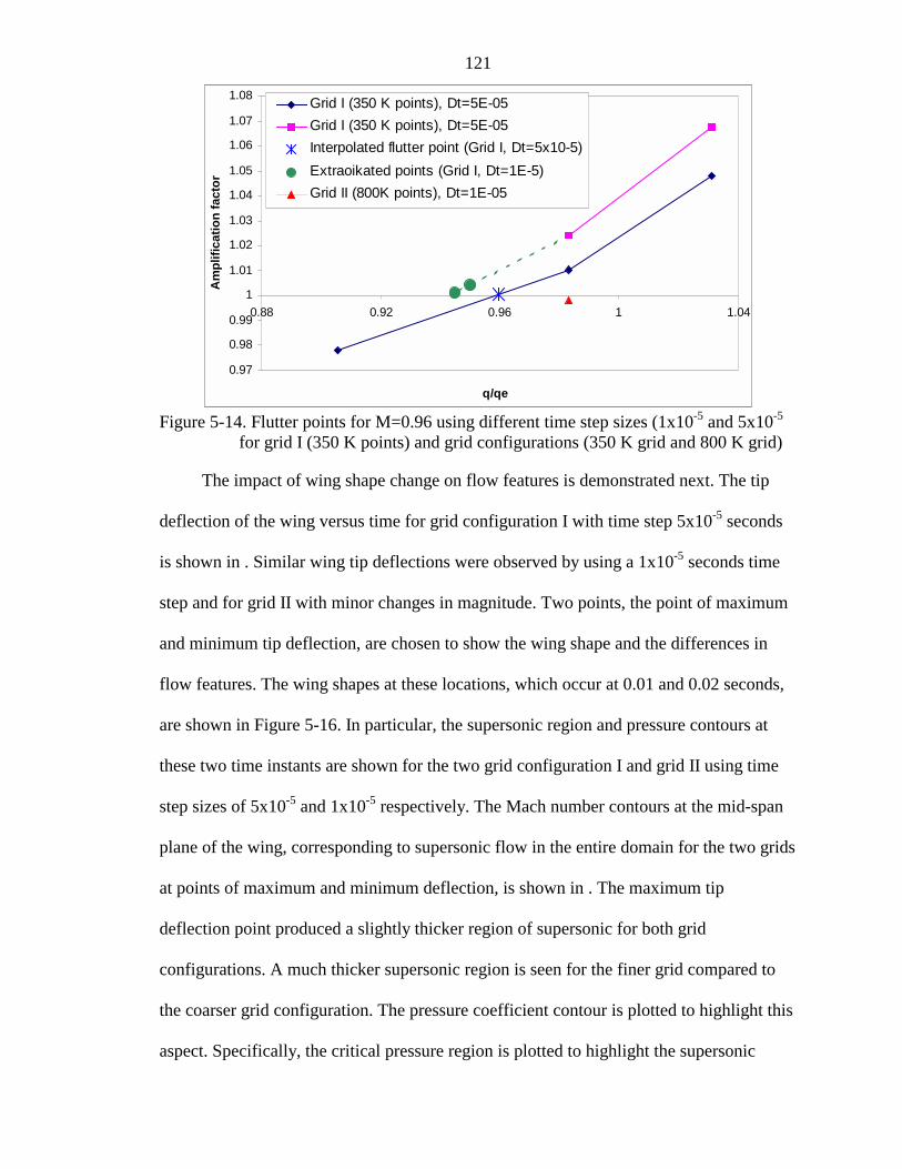
121
Figure 5-14. Flutter points for M=0.96 using different time step sizes (1x10⁻⁵ and 5x10⁻⁵ for grid I (350 K points) and grid configurations (350 K grid and 800 K grid)
The impact of wing shape change on flow features is demonstrated next. The tip
deflection of the wing versus time for grid configuration I with time step 5x10⁻⁵ seconds
is shown in . Similar wing tip deflections were observed by using a 1x10⁻⁵ seconds time
step and for grid II with minor changes in magnitude. Two points, the point of maximum
and minimum tip deflection, are chosen to show the wing shape and the differences in
flow features. The wing shapes at these locations, which occur at 0.01 and 0.02 seconds,
are shown in Figure 5-16. In particular, the supersonic region and pressure contours at
these two time instants are shown for the two grid configuration I and grid II using time
step sizes of 5x10⁻⁵ and 1x10⁻⁵ respectively. The Mach number contours at the mid-span
plane of the wing, corresponding to supersonic flow in the entire domain for the two grids
at points of maximum and minimum deflection, is shown in . The maximum tip
deflection point produced a slightly thicker region of supersonic for both grid
configurations. A much thicker supersonic region is seen for the finer grid compared to
the coarser grid configuration. The pressure coefficient contour is plotted to highlight this
aspect. Specifically, the critical pressure region is plotted to highlight the supersonic
0.97
0.98
0.99
1
1.01
1.02
1.03
1.04
1.05
1.06
1.07
1.08
0.88 0.92 0.96 1 1.04
q/qe
Am
plifi
catio
n fa
ctor
Grid I (350 K points), Dt=5E-05Grid I (350 K points), Dt=5E-05Interpolated flutter point (Grid I, Dt=5x10⁻⁵)Extraoikated points (Grid I, Dt=1E-5)Grid II (800K points), Dt=1E-05
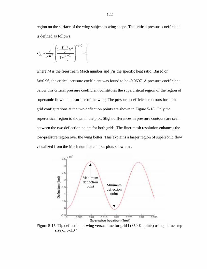
122
region on the surface of the wing subject to wing shape. The critical pressure coefficient
is defined as follows
( )12
2
112 2 111
2
crp
MC
M
− − + = − − +
γ γγ
γγ
where M is the freestream Mach number and γ is the specific heat ratio. Based on
M=0.96, the critical pressure coefficient was found to be -0.0697. A pressure coefficient
below this critical pressure coefficient constitutes the supercritical region or the region of
supersonic flow on the surface of the wing. The pressure coefficient contours for both
grid configurations at the two deflection points are shown in Figure 5-18. Only the
supercritical region is shown in the plot. Slight differences in pressure contours are seen
between the two deflection points for both grids. The finer mesh resolution enhances the
low-pressure region over the wing better. This explains a larger region of supersonic flow
visualized from the Mach number contour plots shown in .
Figure 5-15. Tip deflection of wing versus time for grid I (350 K points) using a time step size of 5x10⁻⁵
Minimum deflection
point
Maximum deflection
point
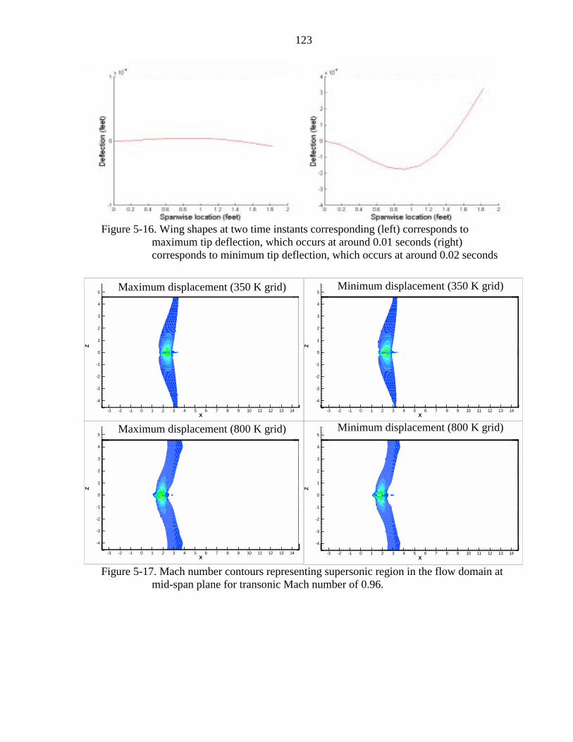
123
Figure 5-16. Wing shapes at two time instants corresponding (left) corresponds to maximum tip deflection, which occurs at around 0.01 seconds (right) corresponds to minimum tip deflection, which occurs at around 0.02 seconds
Figure 5-17. Mach number contours representing supersonic region in the flow domain at mid-span plane for transonic Mach number of 0.96.
X
Z
-3 -2 -1 0 1 2 3 4 5 6 7 8 9 10 11 12 13 14
-4
-3
-2
-1
0
1
2
3
4
5Maximum displacement (350 K grid)
X
Z
-3 -2 -1 0 1 2 3 4 5 6 7 8 9 10 11 12 13 14
-4
-3
-2
-1
0
1
2
3
4
5Minimum displacement (350 K grid)
X
Z
-3 -2 -1 0 1 2 3 4 5 6 7 8 9 10 11 12 13 14
-4
-3
-2
-1
0
1
2
3
4
5Minimum displacement (800 K grid)
X
Z
-3 -2 -1 0 1 2 3 4 5 6 7 8 9 10 11 12 13 14
-4
-3
-2
-1
0
1
2
3
4
5Maximum displacement (800 K grid)
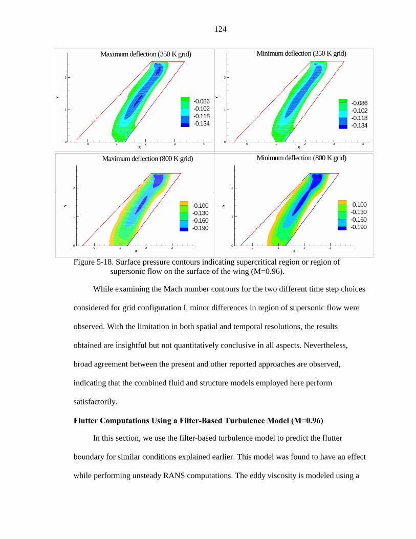
124
Figure 5-18. Surface pressure contours indicating supercritical region or region of supersonic flow on the surface of the wing (M=0.96).
While examining the Mach number contours for the two different time step choices
considered for grid configuration I, minor differences in region of supersonic flow were
observed. With the limitation in both spatial and temporal resolutions, the results
obtained are insightful but not quantitatively conclusive in all aspects. Nevertheless,
broad agreement between the present and other reported approaches are observed,
indicating that the combined fluid and structure models employed here perform
satisfactorily.
Flutter Computations Using a Filter-Based Turbulence Model (M=0.96)
In this section, we use the filter-based turbulence model to predict the flutter
boundary for similar conditions explained earlier. This model was found to have an effect
while performing unsteady RANS computations. The eddy viscosity is modeled using a
X
Y
0 1 2 3 40
1
2
-0.086-0.102-0.118-0.134
Minimum deflection (350 K grid)
X
Y
0 1 2 3 40
1
2
-0.086-0.102-0.118-0.134
Maximum deflection (350 K grid)
-1
0
1
2
3
4
5
X
Y
0 1 2 30
1
2
-0.100-0.130-0.160-0.190
Maximum deflection (800 K grid)
Z
-1
0
1
2
3
4
5
X
Y
0 1 2 30
1
2
-0.100-0.130-0.160-0.190
Minimum deflection (800 K grid)
125
filter, whose size is dependent on the grid size under consideration. The eddy viscosity
model is written here for convenience.
2
3/ 21,tkC Min
kµεµ ρ
ε∆ ⋅ = ⋅
Here, ∆ is the filter size, which has a lower bound as the maximum grid size dimension
so that all scales are numerically resolvable. The blending function, f= 3/ 21,Mink∆ ⋅ε
,
needs to return a value of 1 near the wall regions to enable the use of wall functions
approach. Due to this limitation, we cannot choose too small a filter size. Three different
filter sizes (0.1, 0.15 and 0.2) were chosen initially to determine the distribution of the
blending function in the entire domain. In particular, we wanted to verify whether the
blending function did return a value of 1 near the wing region. A contour plot of blending
function, where it takes a value of 1, at midspan on the wing is shown in Figure 5-19. The
region near the wing cross-section is zoomed in as well to verify that wall functions can
be used in this region. It can be seen from the plot that, for a filter size of 0.1, there are
some regions around the wing, especially near the leading edge, where the blending
function is not 1 and hence not suitable for wall functions approach. Both filter size 0.15
and 0.2 did reproduce the original eddy viscosity model near the wing boundary. A filter
size of 0.15 was chosen as a suitable choice of filter size for all of our computations.
Unsteady computations were performed for only two choices of dynamic pressures
(q/qe=0.905 and 0.98). Computations are carried out using a time step size of 5 x 10⁻⁵
seconds on grid configuration I. Generalized displacement plot for q/qe=0.98 is compared
with the standard k-ε model with wall functions in Figure 5-20. The difference between
the two cases was found to be minimal. The flutter points obtained using filter-based
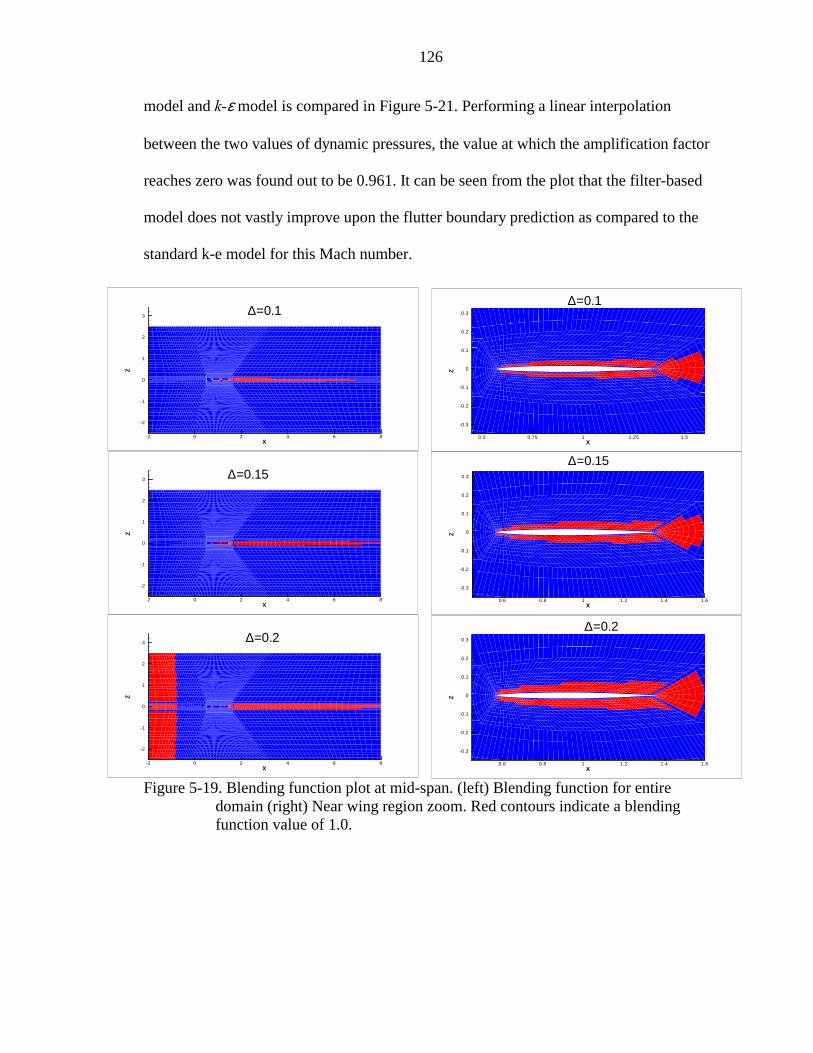
126
model and k-ε model is compared in Figure 5-21. Performing a linear interpolation
between the two values of dynamic pressures, the value at which the amplification factor
reaches zero was found out to be 0.961. It can be seen from the plot that the filter-based
model does not vastly improve upon the flutter boundary prediction as compared to the
standard k-e model for this Mach number.
Figure 5-19. Blending function plot at mid-span. (left) Blending function for entire domain (right) Near wing region zoom. Red contours indicate a blending function value of 1.0.
XZ
0.5 0.75 1 1.25 1.5
-0.3
-0.2
-0.1
0
0.1
0.2
0.3
∆=0.1
X
Z
0.6 0.8 1 1.2 1.4 1.6
-0.3
-0.2
-0.1
0
0.1
0.2
0.3
∆=0.15
X
Z
0.6 0.8 1 1.2 1.4 1.6
-0.3
-0.2
-0.1
0
0.1
0.2
0.3
∆=0.2
X
Z
-2 0 2 4 6 8
-2
-1
0
1
2
3 ∆=0.2
X
Z
-2 0 2 4 6 8
-2
-1
0
1
2
3 ∆=0.15
X
Z
-2 0 2 4 6 8
-2
-1
0
1
2
3 ∆=0.1
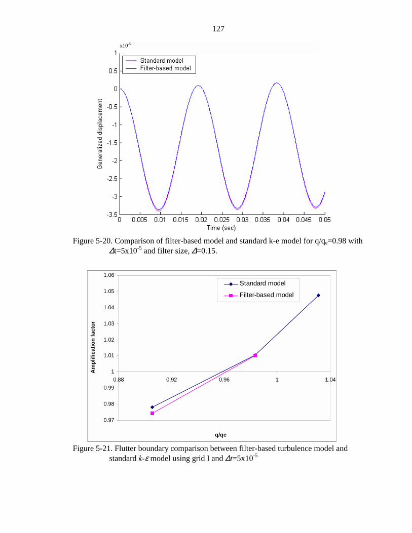
127
Figure 5-20. Comparison of filter-based model and standard k-e model for q/qe=0.98 with ∆t=5x10⁻⁵ and filter size, ∆=0.15.
Figure 5-21. Flutter boundary comparison between filter-based turbulence model and standard k-ε model using grid I and ∆t=5x10⁻⁵
0.97
0.98
0.99
1
1.01
1.02
1.03
1.04
1.05
1.06
0.88 0.92 0.96 1 1.04
q/qe
Am
plifi
catio
n fa
ctor
Standard model
Filter-based model
x10-5
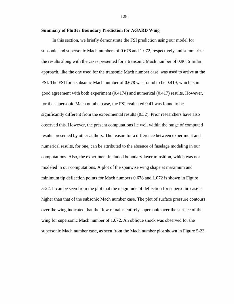
128
Summary of Flutter Boundary Prediction for AGARD Wing
In this section, we briefly demonstrate the FSI prediction using our model for
subsonic and supersonic Mach numbers of 0.678 and 1.072, respectively and summarize
the results along with the cases presented for a transonic Mach number of 0.96. Similar
approach, like the one used for the transonic Mach number case, was used to arrive at the
FSI. The FSI for a subsonic Mach number of 0.678 was found to be 0.419, which is in
good agreement with both experiment (0.4174) and numerical (0.417) results. However,
for the supersonic Mach number case, the FSI evaluated 0.41 was found to be
significantly different from the experimental results (0.32). Prior researchers have also
observed this. However, the present computations lie well within the range of computed
results presented by other authors. The reason for a difference between experiment and
numerical results, for one, can be attributed to the absence of fuselage modeling in our
computations. Also, the experiment included boundary-layer transition, which was not
modeled in our computations. A plot of the spanwise wing shape at maximum and
minimum tip deflection points for Mach numbers 0.678 and 1.072 is shown in Figure
5-22. It can be seen from the plot that the magnitude of deflection for supersonic case is
higher than that of the subsonic Mach number case. The plot of surface pressure contours
over the wing indicated that the flow remains entirely supersonic over the surface of the
wing for supersonic Mach number of 1.072. An oblique shock was observed for the
supersonic Mach number case, as seen from the Mach number plot shown in Figure 5-23.
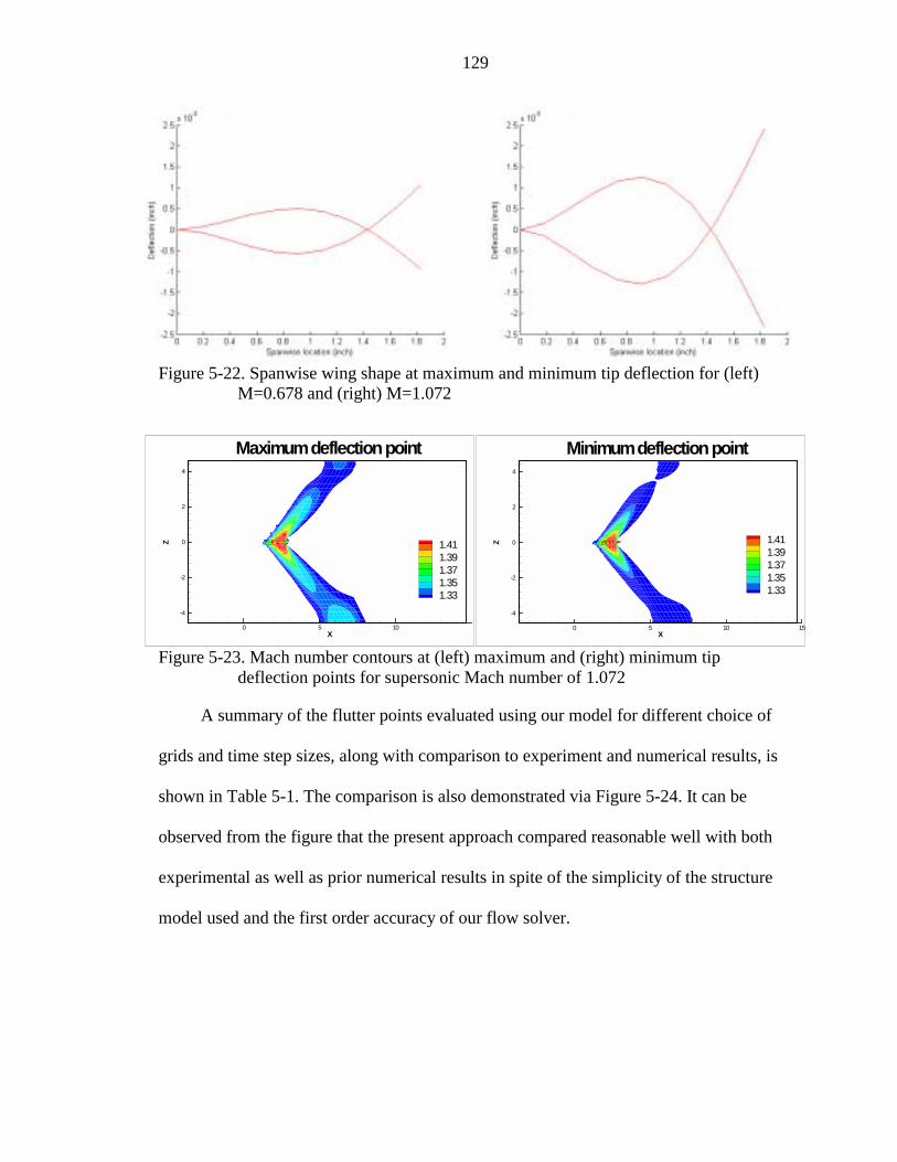
129
Figure 5-22. Spanwise wing shape at maximum and minimum tip deflection for (left) M=0.678 and (right) M=1.072
Figure 5-23. Mach number contours at (left) maximum and (right) minimum tip deflection points for supersonic Mach number of 1.072
A summary of the flutter points evaluated using our model for different choice of
grids and time step sizes, along with comparison to experiment and numerical results, is
shown in Table 5-1. The comparison is also demonstrated via Figure 5-24. It can be
observed from the figure that the present approach compared reasonable well with both
experimental as well as prior numerical results in spite of the simplicity of the structure
model used and the first order accuracy of our flow solver.
X
Z
0 5 10
-4
-2
0
2
4
1.411.391.371.351.33
Maximumdeflectionpoint
X
Z
0 5 10 15
-4
-2
0
2
4
1.411.391.371.351.33
Minimumdeflectionpoint
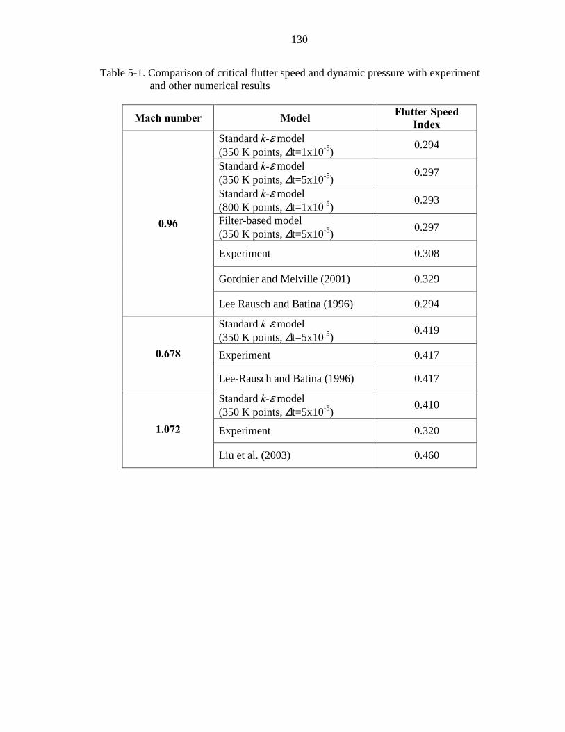
130
Table 5-1. Comparison of critical flutter speed and dynamic pressure with experiment and other numerical results
Mach number Model Flutter Speed Index
Standard k-ε model (350 K points, ∆t=1x10⁻⁵)
0.294
Standard k-ε model (350 K points, ∆t=5x10⁻⁵)
0.297
Standard k-ε model (800 K points, ∆t=1x10⁻⁵)
0.293
Filter-based model (350 K points, ∆t=5x10⁻⁵) 0.297
Experiment 0.308
Gordnier and Melville (2001) 0.329
0.96
Lee Rausch and Batina (1996) 0.294
Standard k-ε model (350 K points, ∆t=5x10⁻⁵) 0.419
Experiment 0.417 0.678
Lee-Rausch and Batina (1996) 0.417
Standard k-ε model (350 K points, ∆t=5x10⁻⁵) 0.410
Experiment 0.320 1.072
Liu et al. (2003) 0.460
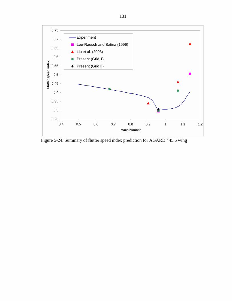
131
Figure 5-24. Summary of flutter speed index prediction for AGARD 445.6 wing
0.25
0.3
0.35
0.4
0.45
0.5
0.55
0.6
0.65
0.7
0.75
0.4 0.5 0.6 0.7 0.8 0.9 1 1.1 1.2Mach number
Flut
ter s
peed
inde
x
Experiment
Lee-Rausch and Batina (1996)
Liu et al. (2003)
Present (Grid 1)
Present (Grid II)
132
CHAPTER 6 CONCLUSIONS AND FUTURE WORK
Conclusions
This work is motivated by our interest in developing a suitable computational
capability to account for fluid and structure interactions to perform computational
aeroelastic analysis on three-dimensional wing geometries. The computational capability
is applied to study both incompressible as well as compressible flow computations
around three-dimensional wing geometries. The aeroelastic phenomenon looked at is the
flutter characteristics for the AGARD 445.6 wing at a transonic Mach number. The
Reynolds-averaged Navier-Stokes equations, cast in their conservation form, along with a
linear structure solver based on beam finite elements and appropriate moving boundary
and interfacing procedures, are employed. The two-equation k-ε model with wall
functions method for near wall treatment is adopted for turbulence closure.
A multi-block, structured flow solver that uses finite volume formulation based on
a pressure-based method was employed to integrate the RANS equations. It is coupled
with linear structure model with beam finite elements that is based on Bernoulli-Euler
beam theory. A predictor-corrector based PISO algorithm was proposed to perform
unsteady computations for the flow solver. This method, being a non-iterative algorithm,
greatly reduces the computational cost of flow computations, which constitutes the major
part of the computational time of the coupled solver. Since it is a semi-implicit method, it
is controlled by the CFL-type stability condition and hence the time step size needed to
be chosen carefully based on the CFL number. A fully implicit Newmark method is used
133
to integrate the modal equations of motion of the structure and hence is not limited by a
time step size. The time step size chosen for the coupled simulation is entirely based on
the flow solver and time-synchronization is ensured between the two modules to prevent
any phase lag.
The two modules are integrated at the interface or boundary using interfacing
techniques. Particularly, a bilinear interpolation technique was used to transfer surface
pressure from flow domain to structure domain and a linear extrapolation is used to
transfer displacement field from structure domain to fluid domain. A robust moving
boundary module based on master/slave concepts and transfinite interpolation method
was embedded into the coupled solver to account for re-meshing of the entire flow
domain once the new surface or geometry under consideration is known. Impact of two
different parameters on the rigidity of grid movement was studied to preserve the
distance of the first node from the wall to enable the use of wall functions approach
associated with our turbulence model. A filter-based model is introduced as well to
improve upon the predictive capability of the standard k-ε two-equation model.
Various issues were addressed while developing this computationally methodology.
Since the computations are performed on a dynamically moving mesh, the geometric
properties need to be conserved as the mesh configuration changes with time. This is
ensured via the geometric conservation law. This, when implemented in curvilinear
coordinates, calls for updating the Jacobians associated with the cell volumes in a
consistent fashion. Four different schemes for updating Jacobian values were examined in
an attempt to arrive at a robust choice for performing moving grid computations. Both
first and second order fully implicit as well as time-averaged evaluation of metrics were
134
considered. Three test cases, two using the 2-D channel flow one using the 3-D elastic
wing, with different Reynolds number, time dependency, and geometry movement were
carried out to assess the performance of the different GCL schemes implemented. The
first order fully implicit method was found to produce the least error norm for all test
cases. The results have demonstrated that the impact of GCL on the solution accuracy is
not simply governed by the formal order of accuracy of the discretization scheme. The
results also show that the choice of fluid flow solver and magnitude of grid movement
strongly affect the GCL scheme for performing aeroelastic computations. Since the first
order fully implicit GCL scheme simplifies the data structure in the code development
effort, we reached a conclusion that this scheme is appropriate in the context of the fluid
flow solver employed.
Another aspect that was probed into was the time dependency effect associated
with the momentum interpolation method, which is required to compute the contravariant
velocity components when using a collocated or non-staggered grid. The original Rhie-
Chow momentum interpolation method was developed with steady state computations in
mind. However, while performing unsteady computations, this scheme was found to
produce spurious oscillations in the pressure and velocity fields especially when a smaller
time step is used. Hence, this scheme needed to be modified to include time dependency
effects to accurately compute the contravariant velocities. The proposed scheme
eliminated any time dependency effect observed with the original scheme and hence was
used for all our future computations.
Coupled simulations are carried out using the AGARD 445.6 wing after taking care
of the above-mentioned issues. Both incompressible as well as compressible flow
135
computations were carried out to study the coupling procedure and to compute the flutter
boundary for the AGARD wing at various Mach numbers. For the incompressible,
turbulent flow computation, the full structure model with all the modes was used. Wing
shapes at different time instants were shown and it was seen that the deflection reaches
steady state after a certain time due to the presence of damping in the structure. We also
showed the time history of aerodynamic parameters and showed that they converged to a
steady state value as well. A grid refinement study was done as well and the aerodynamic
parameters compared with the coarse grid solution. Oscillations in the aerodynamic
parameters were observed before converging towards steady state value. The effect of
angle of attack on the aerodynamic parameters was also looked at for three different
values of angle of attack. Results were found to be in good agreement with theory. An
iterative flow solver based on SIMPLE family of methods was used for all of the above
computations.
The main objective of this thesis was to study flutter characteristics around a three-
dimensional wing. Computations around the AGARD wing were performed at three
different Mach numbers of 0.678, 0.96 and 1.072. All flow computations were performed
using the non-iterative PISO algorithm. The PISO algorithm was validated first by
comparing it with the SIMPLE algorithm using the AGARD wing example for
incompressible flows. Excellent agreement was observed with one another, however, the
computational cost, by using PISO method was improved by ten folds. Only one mode of
the structure is used here to predict the flutter boundary of the wing. The flutter boundary
is predicted by varying the dynamic pressure and by studying the generalized
displacement of the structure. Two grid configurations, one with 350,000 points and
136
another with 800,000 points were considered to study the transonic Mach number case.
Two different time steps were used for the coarser grid to determine the impact of
different time step sizes on solution accuracy. The coarser of the two grids predicted
flutter boundary accurately for subsonic and transonic Mach number cases. but were
found to deviate for supersonic Mach number case. Prior researchers have made such an
observation as well. Computations for transonic Mach number case using the finer grid
showed a closer agreement with experiment compared the coarser grid. The two choice of
time steps on the coarser grid produced some differences in flutter prediction, although
the differences were small, which can be attributed to the first order time marching
scheme employed by the flow solver. Differences in flow features, particularly
supersonic region in the flow domain, were highlighted based on the wing shape
observed at different time instants. This gave insight into the flow physics associated with
deformation in the structure.
The filter-based turbulence was employed as well to perform unsteady flow
computations as the RANS model is tuned by steady state mean flow data and hence was
found to have some shortcomings when dealing with time dependent computations. The
eddy viscosity term was modified using a filter to overcome this. The filter size was so
chosen that wall functions could still be applied near wall regions. Flutter computations
performed using the filter-based model did not show any significant improvement over
the standard k-e model but the results were consistent when compared with the k-ε
model.
To conclude, we have shown that the computational methodology has exhibited
capability to predict flutter characteristics in an accurate manner in spite of coupling a
137
simple linear structure solver with a more complex flow solver. The simulations have
given insight into the flow physics associated with performing a fluid-structure
interaction computation over elastic bodies. It has also given insight into several
numerical issues encountered while carrying out these computations and what needs to be
done to overcome this.
Future Directions
The current research can be extended in the following direction:
• Extend the methodology to investigate nonlinear structural dynamics models to address issues related to larger and more complicated deformation characteristics. Issues such as limit cycle oscillations, buffeting, etc, can be investigated in detail.
• Refine both spatial and temporal resolutions, including possibly adopting higher order time marching schemes. Coupled fluid and structure simulations are very time consuming. Priority should be given to help reduce the computational cost, including higher order schemes, parallel computational capabilities, and adaptively updated grid distributions.
138
LIST OF REFERENCES
Ahlman, D., Söderlund, F., Jackson, J., Kurdila, A., and Shyy, W. (2002) Proper Orthogonal Decomposition for Time-Dependent Lid-Driven Cavity Flows, Numerical Heat Transfer Part B: Fundamentals, v. 42, no. 4, pp. 285-306.
Bathe, K-J (1996) Finite Element Procedures, Prentice Hall, Englewood Cliffs, N. J.
Batina, J. T. (1989) Unsteady Euler Algorithm With Unstructured Dynamic Mesh for Complex-Aircraft Aeroelastic Analysis, AIAA-89-1189.
Bennett, R. M. and Edwards, J. W. (1998) An overview of Recent Developments in Computational Aeroelasticity, AIAA-98-2421.
Bennett, R. M., Batina, J. T. and Cunningham, H. (1989) Wing-Flutter Calculations with the CAP-TSD Unsteady Transonic Small-Disturbance Program, J. Aircraft, v. 26, n. 9, pp. 876-882.
Bhardwaj, M. K., Kapania, K., Reichenbach, E. and Guruswamy, G. P. (1998) Computational Fluid Dynamics/Computational Structural Dynamics Interaction Methodology for Aircraft Wings, AIAA J., v. 36, n.12, pp. 2179-2186.
Bisplingoff, R. L., Ashley, H. and Halfman, R. L. (1955) Aeroelasticity, Dover, New York.
Brown, S. A. (1997) Displacement Extrapolation for CFD+CSD Aeroelastic Analysis, AIAA-97-1090.
Cai, J., Liu, F. and Tsai, H. M. (2001) Static Aero-elastic Computation with a Coupled CFD and CSD Method, AIAA-2001-0717.
Chen, P. C. and Jadic, I. (1998) Interfacing of Fluid and Structural Models via Innovative Structural Boundary Element Method, AIAA J., v. 36, n. 2, pp. 282-287.
Chen, P. C. and Hill, L. R. (1999) A Three- Dimensional Boundary Element Method for CFD/CSD Grid Interfacing, AIAA-99-1213.
Chen, P. C. and Gao, X. W. (2001) A Multi-Block Boundary Element Method for CFD/CSD Grid Interfacing, AIAA-01-0715.
Choi, S. K. (1999) Note on the Use of Momentum Interpolation Method for Unsteady Flows, Numerical Heat Transfer, Part A, v. 36, pp. 545-550.
139
Cunningham. H. J., Batina, J. T. and Bennett, R. M. (1988) Modern Wing Flutter Analysis by Computational Fluid Dynamics Methods, J. Aircraft, v. 25, n. 10, pp. 962-968.
Dowell, E. H. and Hall, K. C. (2001) Modeling of Fluid-Structure Interaction, Ann. Rev. of Fluid Mech.
Eriksson, L. E. (1982) Generation of Boundary-Conformation Grids Around Wing-Body Configurations Using Transfinite Interpolation, AIAA J., v. 20, n. 10, pp. 1313-1320.
Farhat, C., Pierson, K. and Degand, C., (2000) CFD Based Simulation of the Unsteady Aeroelastic Response of a Maneuvering Vehicle, AIAA-2000-0899.
Farhat, C. and Lesoinne, M. (2000) Two efficient staggered algorithms for the serial and parallel solution of three-dimensional nonlinear transient aeroelastic problems, Comput. Methods Appl. Mech. Engrg., v. 182, pp. 499-515.
Farhat, C., Geuzaine, P., Grandmont, C. (2001) The Discrete Geometric Conservation Law and the Nonlinear Stability of ALE Schemes for the solution of Flow Problems on Moving Grids, J. Comput. Phys., v. 174, pp. 669-694.
Farhat, C., Geuzaine, P. and Brown, G. (2003) Application of a three-field nonlinear fluid-structure formulation to the prediction of the aeroelastic parameters of an F-16 fighter, Computers and Fluids, v. 32, pp. 3-29.
Friedmann, P. P. (1999) Renaissance of Aeroeslaticity and Its Future, J. Aircraft, v. 36, n. 1, pp. 105-121.
Fung, Y. C. (1955) An introduction to Aeroelasticity. Dover, New York.
Garica, J. A. and Guruswamy, G. P. (1999) Aeroelastic analysis of Transonic Wings Using Navier-Stokes Equations and a Nonlinear Beam Finite Element Model, AIAA-99-1215.
Geuzaine, P., Brown, G. and Farhat, C. (2002) Three-Field-Based Nonlinear Aeroelastic Simulation Technology: Status and Application to the Flutter Analysis of an F-16 Configuration, AIAA-2002-0870.
Gordnier, R. E. and Melville, R. B. (2000) Transonic Flutter Simulations Using an Implicit Aeroelastic Solver, J. Aircraft, v. 37, n. 5, pp. 872-879.
Guillard, H. and Farhat, C. (2000) On the Significance of the geometric conservation law for flow computations on moving meshes, Comput. Methods Appl. Mech. Engrg., v. 190, pp. 1467-1482.
140
Guruswamy, G. P. (2002) A review of numerical fluids/structures interface methods for computations using high-fidelity equations, Computers and Structures, v. 80, pp. 31-41.
Guruswamy, G. P. and Byun, C. (1994) Direct Coupling of Euler Flow Equations with Plate Finite Element Structures, AIAA J., v. 33, n. 2, pp. 375-377.
Guruswamy, G. P. and Byun, C. (1993) Fluid-Structure Interactions Using Navier-Stokes Flow equations Coupled with Shell Finite Element Structures, AIAA-93-3087.
Hartwich, P. M., and Agrawal, S. (1997) Method for Perturbing Multiblock Patched Grids in Aeroelastic and Design Optimization Applications, AIAA Paper 97-2038.
Hartwich, P., Doobs, S., Arslan, A. and Kim, S., (2000) Navier-Stokes Computations of Limit Cycle Oscillations for a B1-Like Configuration, AIAA-2000-2338.
Huang, W., Ren, Y. and Russell, R. D. (1994) Moving Mesh Methods Based on Moving Mesh Partial Differential Equations, J. Comput. Phys., v. 113, pp. 279-290.
Huang, W. and Russell, R. D. (1999) Moving Mesh Strategy Based on a Gradient Flow Equation for Two-Dimensional Problems, SIAM J. Sci. Comput., v. 20, n. 3, pp. 998-1015.
Huang, W. (2001) Practical Aspects of Formulation and Solution of Moving Mesh Partial Differential Equations, J. Comput. Phys., v. 171, pp. 753-775.
Huttsell, L., Schuster, D., Volk, J., Giesing, J. and Love, M. (2001) Evaluation of Computational Aeroelasticity Codes for Loads and Flutter, AIAA-2001-0569.
Johansen, S. T., Wu, J. and Shyy, W. (2004) Filter-based unsteady RANS computations, Int. J. of Heat and Fluid Flow, v. 25, pp. 10-21.
Issa, R. I. (1985) Solution of the Implicitly Discretised Fluid Flow Equations by Operator-Splitting, J. Comp. Phys., v. 62, pp. 40-65.
Kamakoti, R., Lian, Yongsheng, Regisford, S., Kurdila, A. and Shyy, W. (2002) Computational Aeroelasticity Using a Pressure-Based Solver, AIAA-2002-0869.
Koobus, B. and Farhat, C. (1999) Second-order time-accurate and geometrically conservative implicit schemes for flow computations on unstructured dynamic meshes, Comput. Methods Appl. Mech. Engrg., v. 170, pp. 103-129.
Launder, B. E. and Spalding, D. B. (1974) The Numerical Computations of Turbulent Flows, Comp. Meth. Appl. Mech. Engg., v. 3, pp. 269-289.
Lee-Rausch, E. M. and Batina, J. T. (1996) Wing Flutter Computations Using an Aerodynamic Model Based on the Navier-Stokes Equations, J. Aircraft, v. 33, n. 6, pp. 1139-1147.
141
Lee-Rausch, E. M. and Batina, J. T. (1995) Wing Flutter Boundary Prediction Using Unsteady Aerodynamic Method, J. Aircraft, v. 32, n. 2, pp. 416-422.
Lee-Rausch, E. M. and Batina, J. T. (1993) Calculation of AGARD Wing 445.6 Flutter using Navier-Stokes Aerodynamics, AIAA-93-3476.
Lesoinne, M. and Farhat, C. (1996) Geometric conservation laws for flow problems with moving boundaries and deformable meshes, and their impact on aeroelastic computations, Comput. Methods Appl. Mech. Engrg., v. 134, pp. 71-90.
Lesoinne, M. and Farhat, C. (2001) CFD-Based Aeroelastic Eigensolver for the Subsonic, Transonic, and Supersonic Regimes, J. Aircraft, v. 38, n. 4, pp. 628-635.
Lewis, A. P. and Smith, M. J. (1998) Extension of a Euler/Navier-Stokes Aeroelastic Analysis Method for Shell Structures, AIAA-98-2656.
Liu, F. Sadeghi, M., Yang, S. and Tsai, H. (2003) Parallel Computation of Wing Flutter with a Coupled Navier-Stokes/CSD Method, AIAA-2003-1347.
Liu, F., Cai, J., Zhu, Y., Wong, A. S. F. and Tsai, H. M., (2000) Calculation of Wing Flutter by a Coupled CFD-CSD Method, AIAA-2000-0907.
Morton, S. A., Melville, R. B. and Visbal, M. R. (1998) Accuracy and Coupling Issues of Aeroelastic Navier-Stokes Solutions on Deforming Meshes, J. Aircraft, v. 35, n. 5, pp. 798-805.
Moyroud, F., Cosme, N., Jocker, M., Fransson, T. H., Lornage, D. and Jacquet-Richardet, G. (2000) A Fluid-Structure Interfacing Technique for Computational Aeroelastic Simulations, 9th International Symposium on Unsteady Aerodynamics, Aeroacoustics and Aeroelasticity of Turbomachines, Lyon, France.
Patankar, S. V. and Spalding, D. B. (1972) A calculation procedure for heat, mass and momentum transfer in three-dimensional parabolic flows, Int. J. Heat and Mass Transf., v. 15, pp. 1787-1806.
Potsdam, M. A. and Guruswamy, G. P. (2001) A Parallel Multiblock Mesh Movement Scheme for Complex Aeroelastic Applications, AIAA-2001-0716.
Reuther, J., Jameson, A., Farmer, J., Martinelli, L., and Saunders, D. (1996), Aerodynamics Shape Optimization of Complex Aircraft Configurations via an Adjoint Formulation, AIAA-96-0094.
Rhie, C. M. and Chow, W. L. (1983) Numerical Study of the Turbulent Flow Past an Airfoil with Trailing Edge Separation, AIAA J., v. 21, n. 11, pp. 1525-1535.
Robinson, B. A., Batina, J. T. and Yang, H. T. Y. (1991) Aeroelastic Analysis of Wings Using the Euler Equations with a Deforming Mesh, J. Aircraft, v. 28, n. 11, pp. 781-788.
142
Schuster, D. M., Vadyak, J. and Atta, E. (1990) Static Aeroelastic Analysis of Fighter Aircraft Using a Three-Dimensional Navier-Stokes Algorithm, J. Aircraft, v. 27, n. 9, pp. 820-825.
Schuster, D. M., Liu, D. D. and Huttsell, L. J. (2003) Computational Aeroelasticity: Success, Progress, Challenge, J. Aircraft, v. 40, n. 5, pp. 843-856.
Seigel, J. M., Parthasarathy, V., Kingsley, G. M., Dionne, P. J., Harrand, V. J. and Luker, J. J. (1998) Application of a Multi-Disciplinary Computing Environment (MDICE) for Loosely Coupled Fluid-Structural Analysis, AIAA-98-4865.
Shyy, W. (1994) “Computational Modeling for Fluid Flow and Interfacial Transport”, Elsevier, Amsterdam.
Shyy, W., Udaykumar, H. S., Rao, M. M. and Smith, R. W. (1996) Computational Fluid Dynamics with Moving Boundaries, Taylor and Francis, London.
Shyy, W. & Braaten, M. E. (1988) Application of a Generalized Pressure Correction Algorithm for Flows in Complicated Geometries”, in O. Baysal (ed.), Advances and Applications in Computational Fluid Dynamics, ASME, New York, pp. 109–119.
Shyy, W., Thakur, S.S., Ouyang, H., Liu, J. and Blosch, E. (1997) “Computational techniques for Complex Transport Phenomena”, Cambridge University Press, New York.
Shyy, W., Francois, M., Udaykumar, H.S., N’dri N. and Tran-Son-Tay, R. (2001) Moving Boundaries in Micro-Scale Biofluid Dynamics, Applied Mechanics Reviews, v. 54, pp.419-453.
Smith, M. J., Hodges, D. H. and Cesnik, C. E. S., (2000) Evaluation of computational Algorithms Suitable for Fluid-Structure Interactions, J. Aircraft, v. 37, n. 2, pp. 282-294.
Smith, M. J., Schuster, D. M., Huttsell, L. and Buxton, B. (1996a) Development of an Euler/Navier-Stokes Aeroelastic Method for Three- Dimensional Vehicles with Multiple Flexible Surfaces, AIAA-96-1513-CP.
Smith, M. J., Cesnik, C. E. S., Hodges, D. H. and Moran, K. J. (1996b) An Evaluation of Computational algorithms to Interface Between CFD and CSD Methodologies, AIAA-96-1400.
Thakur, S. and Wright, J. (2004) A Multiblock Operator-Splitting Algorithm for Unsteady Flows at all Speeds in Complex Geometries, Accepted for publication to Int. J. of Num. Methods in Fluids.
143
Thakur, S. Wright, J. and Shyy, W. (2002) “STREAM: A Computational Fluid Dynamics and Heat Transfer Navier-Stokes Solver: Theory and Applications.” Streamline Numerics, Inc., Gainesville, Florida.
Thomas, P. D. and Lombard, K. (1979) Geometric Conservation Law and Its Application to Flow Computations on Moving Grids, AIAA J., v. 17, n. 10, pp. 1030-1037.
Tsai, H.M., Wong, A.S.F., Cai, J., Zhu, Y. and Liu, F. (2000) Unsteady Flow Calculations with a Multi-Block Moving Mesh Algorithm, AIAA-2000-1002.
Williamson, C. H. K. (1989) Oblique and Parallel Mode of Vortex Shedding in the Wake of a Cylinder at Low Reynolds Number, J. Fluid Mech., v. 206, pp. 579-627.
Wong, A., Tsai, H., Cai, J., Zhu, Y. and Liu, F. (2000) Unsteady Flow Calculations with a Moving Mesh Algorithm, AIAA-2000-1002.
Yates, E. C., Jr., (1987) AGARD Standard Aeroelastic Configuration for Dynamic Response, Candidate Configuration I.-Wing 445.6, NASA TM 100492.
Yates, E. C. Jr., Land, N. S. and Foughner, J. T. Jr. (1963) Measured and Calculated Subsonic and Transonic Flutter Characteristics of a 45o Sweptback Wing Planform in Air and in Freon-12 in the Langley Transonic Dynamics Tunnel, AGARD TN D-1616.
Yu, B., Kawaguchi, Y., Tao, W. Q. and Ozoe, H. (2002a) Checkerboard Pressure Predictions Due to Underrelaxation Factor and Time Step Size for a Nonstaggered Grid with Momentum Interpolation Method, Numerical Heat Transfer, Part B, v. 41, pp. 85-94.
Yu, B., Tao, W. Q., Wei, J. J., Kawaguchi, Y., Tagawa, T. and Ozoe, H. (2002b) Discussion on momentum interpolation method for collocated grids of incompressible flow, Numerical Heat Transfer, Part B, v. 42, pp. 141-166.
Zhang, B., Lian, Y. and Shyy, W. (2003) Proper Orthogonal Decomposition for Three-Dimensional Membrane Wing Aerodynamics, AIAA-2003-3917.
144
BIOGRAPHICAL SKETCH
Ramji Kamakoti was born in 1976, in the historic city of Pondicherry in India
(although he was brought up in Chennai). He received his bachelor’s degree in
mechanical engineering from the Birla Institute of Technology and Science, located in a
place called Pilani, in the state of Rajasthan. He then decided to come to the US for
graduate studies in the field of engineering mechanics at the University of Florida, where
he obtained his master’s degree in 2000. For the previous 6 years, he did research in the
field of fluid-structure interaction (in the computational thermo-fluids group under the
guidance of professor Wei Shyy).