Compressed RF Tomography for Wireless Sensor …mrabba1/pubs/2009/mohammad_dcoss09.pdf · Compressed RF Tomography for Wireless Sensor Networks: Centralized and Decentralized Approaches

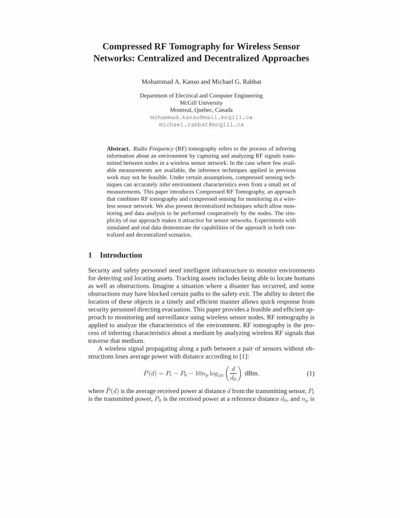
Compressed RF Tomography for Wireless SensorNetworks: Centralized and Decentralized Approaches

Mohammad A. Kanso and Michael G. Rabbat

Department of Electrical and Computer EngineeringMcGill University

Montreal, Quebec, [email protected]

[email protected]

Abstract. Radio Frequency (RF) tomography refers to the process of inferringinformation about an environment by capturing and analyzing RF signals trans-mitted between nodes in a wireless sensor network. In the case where few avail-able measurements are available, the inference techniquesapplied in previouswork may not be feasible. Under certain assumptions, compressed sensing tech-niques can accurately infer environment characteristics even from a small set ofmeasurements. This paper introduces Compressed RF Tomography, an approachthat combines RF tomography and compressed sensing for monitoring in a wire-less sensor network. We also present decentralized techniques which allow mon-itoring and data analysis to be performed cooperatively by the nodes. The sim-plicity of our approach makes it attractive for sensor networks. Experiments withsimulated and real data demonstrate the capabilities of theapproach in both cen-tralized and decentralized scenarios.

1 Introduction

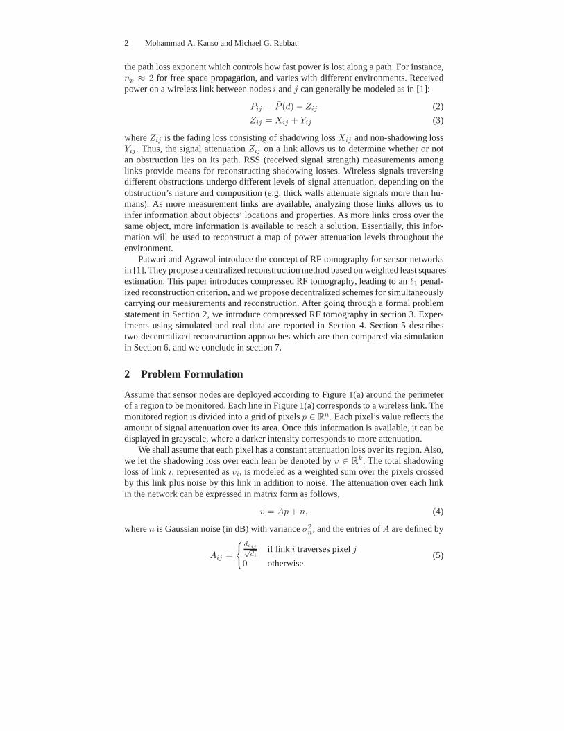
Security and safety personnel need intelligent infrastructure to monitor environmentsfor detecting and locating assets. Tracking assets includes being able to locate humansas well as obstructions. Imagine a situation where a disaster has occurred, and someobstructions may have blocked certain paths to the safety exit. The ability to detect thelocation of these objects in a timely and efficient manner allows quick response fromsecurity personnel directing evacuation. This paper provides a feasible and efficient ap-proach to monitoring and surveillance using wireless sensor nodes. RF tomography isapplied to analyze the characteristics of the environment.RF tomography is the pro-cess of inferring characteristics about a medium by analyzing wireless RF signals thattraverse that medium.

A wireless signal propagating along a path between a pair of sensors without ob-structions loses average power with distance according to [1]:

P (d) = Pt − P0 − 10np log10

(d

d0

)

dBm, (1)

whereP (d) is the average received power at distanced from the transmitting sensor,Pt

is the transmitted power,P0 is the received power at a reference distanced0, andnp is

2 Mohammad A. Kanso and Michael G. Rabbat

the path loss exponent which controls how fast power is lost along a path. For instance,np ≈ 2 for free space propagation, and varies with different environments. Receivedpower on a wireless link between nodesi andj can generally be modeled as in [1]:

Pij = P (d) − Zij (2)

Zij = Xij + Yij (3)

whereZij is the fading loss consisting of shadowing lossXij and non-shadowing lossYij . Thus, the signal attenuationZij on a link allows us to determine whether or notan obstruction lies on its path. RSS (received signal strength) measurements amonglinks provide means for reconstructing shadowing losses. Wireless signals traversingdifferent obstructions undergo different levels of signalattenuation, depending on theobstruction’s nature and composition (e.g. thick walls attenuate signals more than hu-mans). As more measurement links are available, analyzing those links allows us toinfer information about objects’ locations and properties. As more links cross over thesame object, more information is available to reach a solution. Essentially, this infor-mation will be used to reconstruct a map of power attenuationlevels throughout theenvironment.

Patwari and Agrawal introduce the concept of RF tomography for sensor networksin [1]. They propose a centralized reconstruction method based on weighted least squaresestimation. This paper introduces compressed RF tomography, leading to an 1 penal-ized reconstruction criterion, and we propose decentralized schemes for simultaneouslycarrying our measurements and reconstruction. After goingthrough a formal problemstatement in Section 2, we introduce compressed RF tomography in section 3. Exper-iments using simulated and real data are reported in Section4. Section 5 describestwo decentralized reconstruction approaches which are then compared via simulationin Section 6, and we conclude in section 7.

2 Problem Formulation

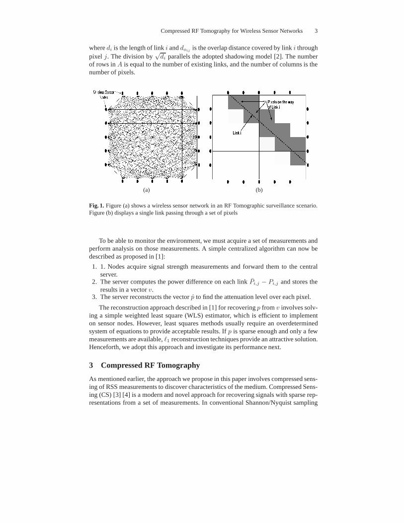
Assume that sensor nodes are deployed according to Figure 1(a) around the perimeterof a region to be monitored. Each line in Figure 1(a) corresponds to a wireless link. Themonitored region is divided into a grid of pixelsp ∈ R

n. Each pixel’s value reflects theamount of signal attenuation over its area. Once this information is available, it can bedisplayed in grayscale, where a darker intensity corresponds to more attenuation.

We shall assume that each pixel has a constant attenuation loss over its region. Also,we let the shadowing loss over each lean be denoted byv ∈ R

k. The total shadowingloss of link i, represented asvi, is modeled as a weighted sum over the pixels crossedby this link plus noise by this link in addition to noise. The attenuation over each linkin the network can be expressed in matrix form as follows,

v = Ap + n, (4)

wheren is Gaussian noise (in dB) with varianceσ2n, and the entries ofA are defined by

Aij =

{doij√

diif link i traverses pixelj

0 otherwise(5)

Compressed RF Tomography for Wireless Sensor Networks 3

wheredi is the length of linki anddoijis the overlap distance covered by linki through

pixel j. The division by√

di parallels the adopted shadowing model [2]. The numberof rows inA is equal to the number of existing links, and the number of columns is thenumber of pixels.

(a) (b)

Fig. 1. Figure (a) shows a wireless sensor network in an RF Tomographic surveillance scenario.Figure (b) displays a single link passing through a set of pixels

To be able to monitor the environment, we must acquire a set ofmeasurements andperform analysis on those measurements. A simple centralized algorithm can now bedescribed as proposed in [1]:

1. 1. Nodes acquire signal strength measurements and forward them to the centralserver.

2. The server computes the power difference on each linkPi,j − Pi,j and stores theresults in a vectorv.

3. The server reconstructs the vectorp to find the attenuation level over each pixel.

The reconstruction approach described in [1] for recoveringp from v involves solv-ing a simple weighted least square (WLS) estimator, which isefficient to implementon sensor nodes. However, least squares methods usually require an overdeterminedsystem of equations to provide acceptable results. Ifp is sparse enough and only a fewmeasurements are available,`1 reconstruction techniques provide an attractive solution.Henceforth, we adopt this approach and investigate its performance next.

3 Compressed RF Tomography

As mentioned earlier, the approach we propose in this paper involves compressed sens-ing of RSS measurements to discover characteristics of the medium. Compressed Sens-ing (CS) [3] [4] is a modern and novel approach for recoveringsignals with sparse rep-resentations from a set of measurements. In conventional Shannon/Nyquist sampling


theorems, a bandlimited signal needs to be sampled at doubleits bandwidth for perfectreconstruction. Compressed sensing shows that undersampling a sparse signal at a ratewell below its Nyquist rate may allow perfect recovery of allsignal components undercertain conditions. Due to the assumption of few changes in our environment (i.e. sparsep), compressed sensing applies naturally. This assumption may hold, for example, inborder monitoring or nighttime security monitoring at a bank. In these examples fewchanges are expected at any given time, which means that onlya few pixels will containsignificant attenuation levels. With this in mind, compressed sensing can be combinedwith RF Tomography to enable monitoring with fewer requiredmeasurements.

An m-sparse signal is a signal that contains maximum ofm nonzero elements. Atypical signal of lengthn and at mostm non-zero components(m � n) requires iterat-ing all elements of the signal elements to determine the few nonzero components. Thechallenging aspect is the recovery of the original signal from the set of measurements.In general, this type of recovery is possible under certain conditions on the measure-ment matrix [3]. This reconstruction occurs with a success probability which increasesas the sparsity level in the signal increases. The prior knowledge of the sparsity of a vec-tor p allows us to reconstruct it from another vectorv of k measurements, by solving anoptimization problem,

p = argminp

||p||0 subject tov = Ap, (6)

whereA is defined above, and||p||0 is defined as the number of nonzero elements inp. Unfortunately, equation (6) is a non-convex NP-hard optimization problem to solveand is computationally intractable. Reconstructing the signal requires iterating through(

nm

)sparse subspaces [5]. Researchers [3, 6, 4] have shown that an easier and equivalent

problem to (6) can be solved:

p = arg minp

||p||1 subject tov = Ap (7)

where ||p||1 is now the`1 norm of p defined as||p||1 =∑n

i=1 |pi|. The optimiza-tion problem in (7) is a convex optimization problem, for which there are numerousalgorithms to compute the solution [3, 7]. Among the first used solutions was linearprogramming, also referred to as Basis Pursuit [3], which requiresO{m log(n)} mea-surements to reconstruct anm-sparse signal.

In practical applications, measured signals are perturbedby noise as in (4). In thissituation, (7) becomes in appropriate for estimatingp since the solution should takethe perturbation into account. The Least Absolute Shrinkage and Selection Operator(LASSO) [8, 9] is a popular sparse estimation technique which solves

p = arg minp

λ‖p‖1 +1

2‖v − Ap‖2

2, (8)

whereλ regulates the tradeoff between sparsity and signal intensity. Note that thismethod requires no prior knowledge of the noise power in the measurements.

Alternatively, iterative greedy algorithms such as Orthogonal Matching Pursuit (OMP)exist [10]. OMP is characterized for being more practical for implementation and faster


than`1-minimization approaches. The tradeoff is the extra numberof measurementsneeded and less robustness to noise in data. A detailed description of the algorithmcan be found in [10]. OMP is particularly attractive for sensor network applicationssince it is computationally simple to implement. However, LASSO can still be a feasi-ble solution, especially when reconstruction only happenson a more powerful receiver.For this, we choose to compare the performance of both centralized techniques in oursimulations and show their tradeoffs.

4 Simulations and Results: Centralized Reconstruction

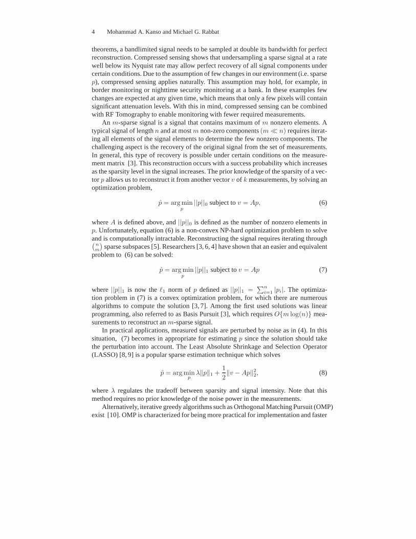
This section presents an evaluation of Compressed RF Tomography. We present resultsfrom computerized simulations as well as some results from real sensor data. The pri-mary focus is on the accuracy of results obtained by a compressed set of measurements.Accuracy in this case is measured in terms of mean squared error of the reconstructedsignal. For better visibility, the recovered values inp from the reconstruction techniqueare mapped onto a vectorp whose values are in [0,1]. Mapping can be a simple lineartransformation onto [0,1], or by a nonlinear transformation as in [1] for better contrast.This allows an easy representation ofp on a grayscale as in Figure 2.

(a) A monitored area with few obstructions discovered(σ2

n=0.01dB

2)

(b) A monitored area with few obstructions (σ2

n=0.49dB

2)

Fig. 2. Simulated environment under surveillance showing the discovered obstructions


The area under simulation is a square area surrounded by 20 sensor nodes, trans-mitting to each other. Each node exchanges information one way with 15 other nodes,as shown in Figure 1(a). This yields a total of20×15

2 = 150 possible links. Figure 2illustrates how our approach can monitor an environment with 30 links at differencenoise levels. The figure shows dark pixels at 4 different positions, each correspondingto an existing obstructions at its location.

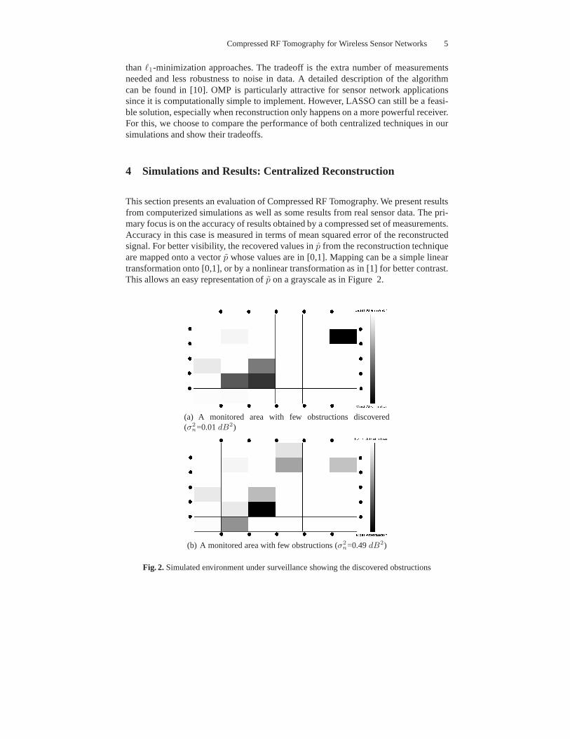
Fig. 3. Performance Comparison of LASSO and OMP with 15 measurements (total=150)

Next we turn our attention to examining the effect of noisy measurements on theperformance of the design. To have a better insight into the amount of error causedby noise, the accuracy of the system is compared to the very low noise (effectivelynoiseless) case. Accuracy is measured by the mean squared error (MSE). We try tomonitor the same obstructions as in Figure 2, with noise alsoadded to measurements toexamine its effect on accuracy. Performance results are plotted in Figure 3. As the figureshows, noise level is reflected on the accuracy of measurements. High noise levels causeinaccuracies in measurements and hence higher MSEs. At lower noise levels, accuratemonitoring is realized, even with few measurements. Note that at low noise levels , theMSE becomes more affected by the few number of measurements available (only 30 inthis case). Comparing the performance of LASSO and OMP techniques, it is obviousthat LASSO performs better, especially when noise levels are high. Results show thatOMP and LASSO techniques behave similar results with low noise, which leads tofavoring the less complex OMP at such conditions. Even at high noise levels, one canstill monitor some of the obstructions.

Compressed RF tomography is well-suited to the case where measurements areavailable. This scenario can occur when some nodes are put tosleep to save batterypower, or when some of the sensors malfunction, or even when links are dropped. Todemonstrate the power of the reconstruction algorithm, we simulate the same obstruc-tion scenario in Figure 2 with a varying number of links used (out of the total 150 linkmeasurements).


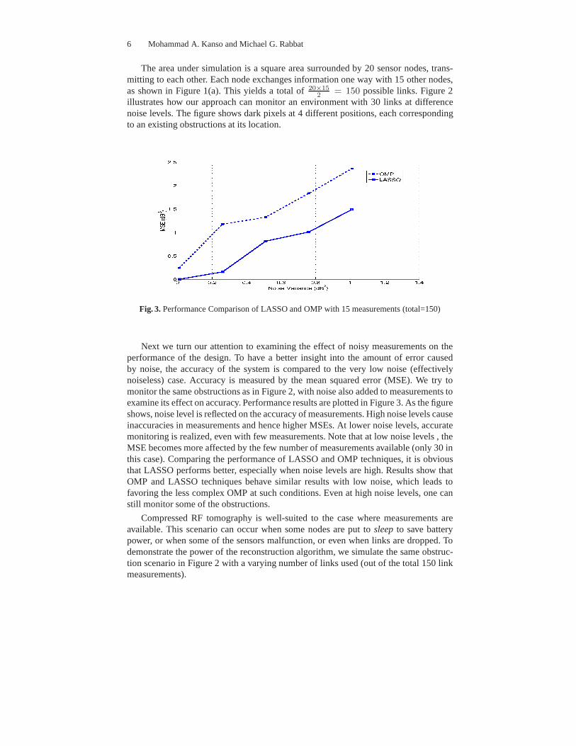
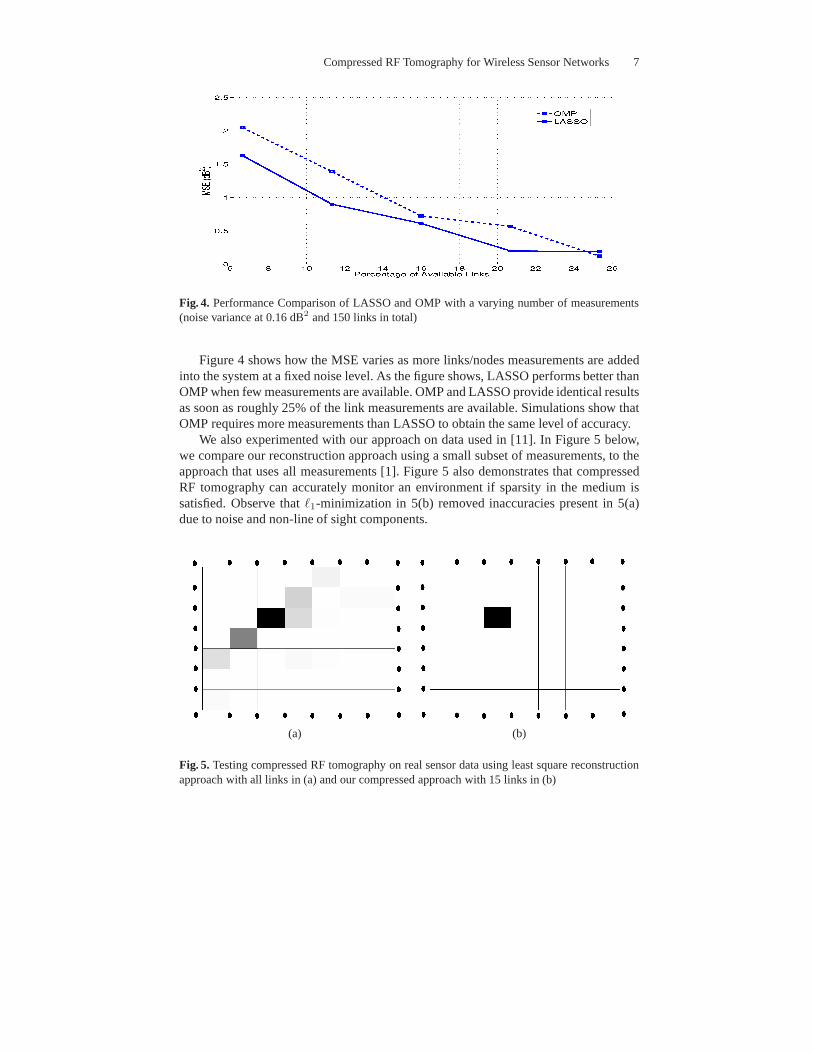
Fig. 4. Performance Comparison of LASSO and OMP with a varying number of measurements(noise variance at 0.16 dB2 and 150 links in total)

Figure 4 shows how the MSE varies as more links/nodes measurements are addedinto the system at a fixed noise level. As the figure shows, LASSO performs better thanOMP when few measurements are available. OMP and LASSO provide identical resultsas soon as roughly 25% of the link measurements are available. Simulations show thatOMP requires more measurements than LASSO to obtain the samelevel of accuracy.

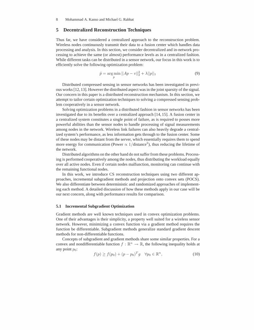
We also experimented with our approach on data used in [11]. In Figure 5 below,we compare our reconstruction approach using a small subsetof measurements, to theapproach that uses all measurements [1]. Figure 5 also demonstrates that compressedRF tomography can accurately monitor an environment if sparsity in the medium issatisfied. Observe that`1-minimization in 5(b) removed inaccuracies present in 5(a)due to noise and non-line of sight components.

(a) (b)

Fig. 5. Testing compressed RF tomography on real sensor data using least square reconstructionapproach with all links in (a) and our compressed approach with 15 links in (b)


5 Decentralized Reconstruction Techniques

Thus far, we have considered a centralized approach to the reconstruction problem.Wireless nodes continuously transmit their data to a fusioncenter which handles dataprocessing and analysis. In this section, we consider decentralized and in-network pro-cessing to achieve the same (or almost) performance levels as in a centralized fashion.While different tasks can be distributed in a sensor network, our focus in this work is toefficiently solve the following optimization problem:

p = arg minp

||Ap − v||22 + λ||p||1 (9)

Distributed compressed sensing in sensor networks has beeninvestigated in previ-ous works [12, 13]. However the distributed aspect was in thejoint sparsity of the signal.Our concern in this paper is a distributed reconstruction mechanism. In this section, weattempt to tailor certain optimization techniques to solving a compressed sensing prob-lem cooperatively in a sensor network.

Solving optimization problems in a distributed fashion in sensor networks has beeninvestigated due to its benefits over a centralized approach[14, 15]. A fusion center ina centralized system constitutes a single point of failure,as is required to posses morepowerful abilities than the sensor nodes to handle processing of signal measurementsamong nodes in the network. Wireless link failures can also heavily degrade a central-ized system’s performance, as less information gets through to the fusion center. Someof these nodes may be distant from the server, which essentially requires them to spendmore energy for communication (Power∝ 1/distance2), thus reducing the lifetime ofthe network.

Distributed algorithms on the other hand do not suffer from these problems. Process-ing is performed cooperatively among the nodes, thus distributing the workload equallyover all active nodes. Even if certain nodes malfunction, monitoring can continue withthe remaining functional nodes.

In this work, we introduce CS reconstruction techniques using two different ap-proaches, incremental subgradient methods and projectiononto convex sets (POCS).We also differentiate between deterministic and randomized approaches of implement-ing each method. A detailed discussion of how these methods apply in our case will beour next concern, along with performance results for comparison.

5.1 Incremental Subgradient Optimization

Gradient methods are well known techniques used in convex optimization problems.One of their advantages is their simplicity, a property wellsuited for a wireless sensornetwork. However, minimizing a convex function via a gradient method requires thefunction be differentiable. Subgradient methods generalize standard gradient descentmethods for non-differentiable functions.

Concepts of subgradient and gradient methods share some similar properties. For aconvex and nondifferentiable functionf : R

n → R, the following inequality holds atany pointp0:

f(p) ≥ f(p0) + (p − p0)T g ∀p0 ∈ R

n, (10)


where theg ∈ Rn is a subgradient off . The set of all subgradients off(p) at any pointp

is called thesubdifferential of f atp, denoted∂f(p). Note that whenf is differentiable,∂f(p) = ∇f(p), i.e. then the gradient becomes the only possible subgradient.

Incremental subgradient methods, originally introduced by [16], split the cost func-tion into smaller functions. The algorithm works iteratively over a set of constraints bysequentially taking steps along the subgradients of those cost functions. For the specialcase of a sensor network environment, the incremental process iterates through mea-surements acquired at each node to converge to the solution at all nodes.

For distributing the optimization task among sensor nodes,the cost function in (9)is split into smaller component functions. Assuming there are N sensor nodes in totalin the network, those nodes gather measurements not necessarily uniformly distributed.Our problem can now be written as

p = arg minp

||Ap − v||22 + λ||p||1

= arg minp

N∑

i=1

∑

j∈Mi

((Ap)j − vj)2 +

λ

N||p||1

︸︷︷︸

fi(p)

(11)

whereMi is the number of RSS measurements acquired by nodei. In each cycle, allnodes iteratively changep in a sequence of subiterations.

The update equation in a decentralized subgradient approach now becomes

p(c+1) = p(c) + µgi(p(c)), (12)

whereµ is a step size,c is an iteration number,gi(p(c)) is the subgradient offi(p) at

p(c) at nodei.Rates of convergence have been analyzed in detail by Nedic and Bertsekas [17].

They show that under certain conditions the algorithm is guaranteed to converge to anoptimal value. However convergence results depend on the approach in choosing thestep sizeµ as well as whether iterations are performed deterministically (round-robinfashion for instance) or randomly. In a deterministic approach, nodes perform updatesin a certain cycle. On the other hand, the updating node in a randomized approach ischosen in a uniformly distributed fashion, saving the requirement to implement a cycle.

Assuming that each sensori acquires a set of measurementsvi via its sensing matrixAi, the subgradient that each node uses in its update equation can be expressed as

gi(pw) =

(2ATi (Aip − vi))w + λ

Nsgn(pw), pw 6= 0

(2ATi (Aip − vi))w + λ

N, pw = 0, (2AT

i (Aip − vi))w < − λN

(2ATi (Aip − vi))w − λ

N, pw = 0, (2AT

i (Aip − vi))w > λN

0, otherwise,(13)

wheresgn(·) is the sign function, and(x)w is elementw of vectorx.


5.2 Projection on Convex Sets (POCS) Method

In addition to the incremental subgradient algorithm discussed earlier, we propose a dis-tributed POCS method suited for a sensor network environment. One important draw-back of subgradient algorithms is that they might converge to local optima or saddlepoints, and can suffer from slow convergence if step sizes are not properly set. The rateof convergence is more relevant to our setup. As simulationswill demonstrate, POCSprovides a feasible solution to this problem, with an additional price of complexity. Thebasic idea of POCS is that data is projected iteratively on the set of constraints. Perhapsone interesting benefit of this method is that it allows adding more constraints to the op-timization problem without significantly changing the algorithm. Furthermore, POCSis known to converge much faster than incremental subgradient algorithms. POCS hasbeen used in the area of image processing [18]. In the area of compressed sensing,POCS methods were employed for data reconstruction [6] but not in a distributed fash-ion.

Let B be`1 ball such that

B = {p ∈ Rn|||p||1 ≤ ||p∗||1}, (14)

and, letH be the hyperplane such that

H = {p ∈ Rn|Ap = v}. (15)

Reconstructed data is required to explain the observationsv and possess sparse fea-tures. SetsH andB attempt to enforce these requirements. Since both sets are convex,the algorithm performs projections onH andB in an alternate fashion. Perhaps one ofthe challenges is projecting onH since it requires solving

argminp

||Ap − v||. (16)

Fortunately, we know this is a simple optimization problem and can be expressed in acompact form via the pseudoinverse (Moore-Penrose inverse).

Since each sensori acquires a set of measurementsvi via a sensing matrixAi,then the POCS algorithm can be iteratively run for every node. In other words, thehyperplaneH now becomes the union of hyperplanesHi = {p ∈ R

n|Ap = v}. Eachnode performs an alternate projection onB andHi and broadcasts the result in thesensor network. The projection on a hyperplaneHi can be expressed as

projHi(x) = x + A+

i (vi − Aix), (17)

whereA+i is the pseudo-inverse ofAi. Note that the hyperplane projection step in [6]

involved the inverse of(AAT )−1 instead of a pseudo-inverse. However, the sensingmatrices used throughout yield uninvertible matrices(AAT )−1, so naturally we decidedto use the pseudo-inverse. Finding the pseudo-inverse requires performing the singularvalue decomposition (SVD) of the matrix. The projection onB is essentially a soft-thresholding step, and is expressed as

projB(x) =

x − λ if x > λ

x + λ if x < −λ

0 otherwise

(18)


5.3 Centralized and Decentralized Tradeoffs

The formulation of our decentralized approach in (11) has the attractive property thatit can be run in parallel among the nodes. Since the objectivefunction is expressedas a sum of separate components, each node can independentlywork on a component.However, each node must have an updated value forp on each iteration. A decentralizedimplementation would involve a node performing an update onp, using incrementalsubgradient or POCS techniques, and then broadcasting thisnew value to all the othernodes. Note that gathering RSS measurements and broadcasting p can be done at thesame time, saving battery power. No other communication is required, since each nodeacquires its own measurements inv and has its own fixed entries in matrixA. So, thecommunication overhead is acceptable in a wireless sensor network.

In a network ofN total sensor nodes, a single iteration in a centralized schemeis equivalent toN (or an average ofN in a randomized setting) iterations in a de-centralized scheme. The centralized approach involves transmittingO(k) values, forkRSS measurements in the network. But compressed sensing theory indicates thatk =O(m log n), wherem is the number of nonzero elements inp. This means that central-ized communication involves transmittingO(m log n) values per iteration.

In a decentralized setting, a single iteration involves each node sending an updatedversion ofp. At mostO(Nn) values are transmitted, wheren is the dimension ofp(generallyN < n). But sincep is a sparse vector, basic data compression methods candecrease packet sizes toO(Nm). Also, since the application of RF tomography requiresall nodes to communicate with each other, then no extra routing costs are required tobroadcastp throughout the network. ComparingO(m log n) to O(Nm) and observingthat generallylog n < N , shows that more communication is required in decentralizedapproaches. Interestingly, one can notice that ifn is large enough (large number ofpixels), decentralized processing would require less communication than centralizedprocessing. Nevertheless, nodes will still spend more battery power to perform iterativeupdates onp. These local computations consist of simple matrix operations as describedearlier.

From an energy point of view, a centralized approach will generally provide fewercommunication overhead, longer network lifetime, and faster processing since all in-formation is gathered at the beginning of the first iteration. However, for practicalityreasons, a decentralized scheme provides more robustness to server and link failures.An optimal approach would be a combination of both centralized and decentralizedtechniques in a hybrid architecture, to exploit the advantages of each technique simul-taneously.

6 Simulations and Discussion: The Decentralized Approach

Using the same environment in Figure 2, we simulate our distributed algorithms forcompressed RF tomographic imaging. Since there is no prior information about themonitored environment, the algorithms are initialized with zero data. One hidden ad-vantage in the algorithms proposed is that they can be run inwarm start mode, con-tinuing from results of previous iterations. So if there is no significant motion in theenvironment, one can expect faster convergence rates.


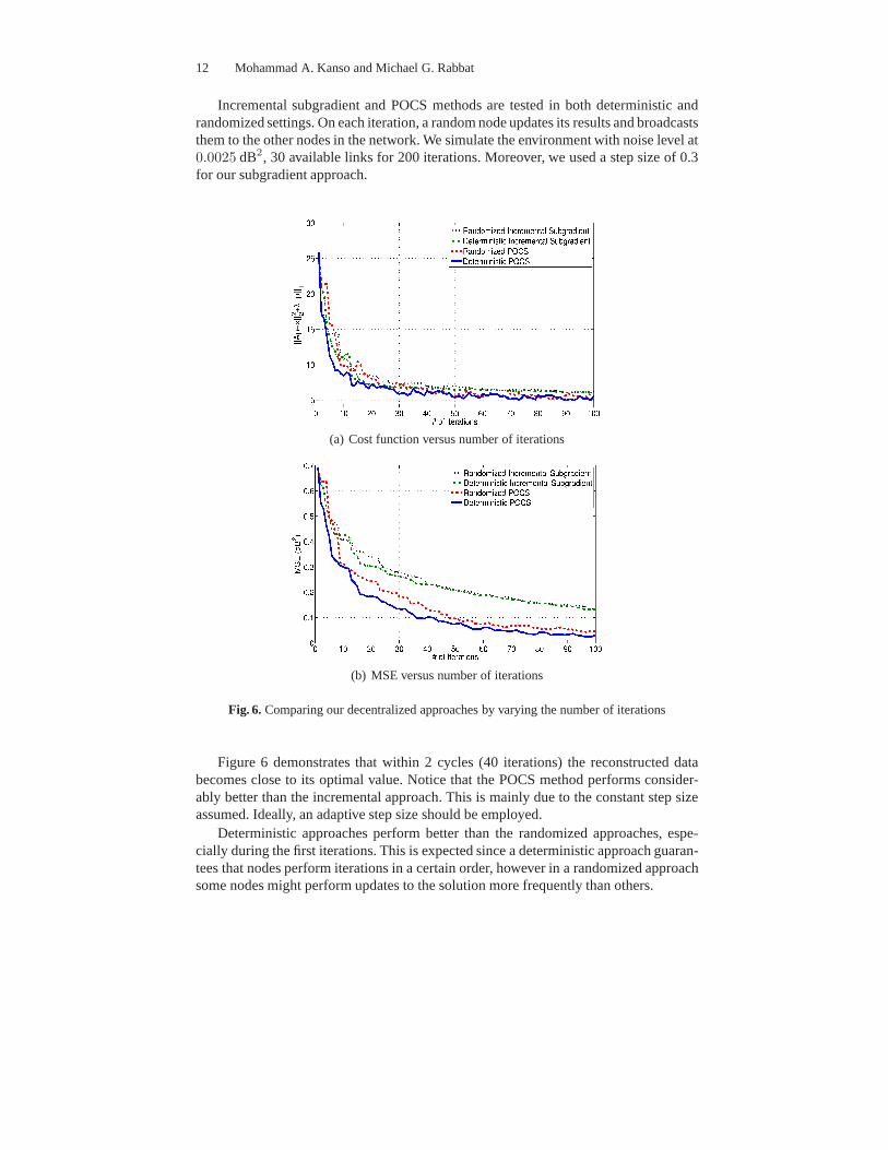
Incremental subgradient and POCS methods are tested in bothdeterministic andrandomized settings. On each iteration, a random node updates its results and broadcaststhem to the other nodes in the network. We simulate the environment with noise level at0.0025 dB2, 30 available links for 200 iterations. Moreover, we used a step size of 0.3for our subgradient approach.

(a) Cost function versus number of iterations

(b) MSE versus number of iterations

Fig. 6. Comparing our decentralized approaches by varying the number of iterations

Figure 6 demonstrates that within 2 cycles (40 iterations) the reconstructed databecomes close to its optimal value. Notice that the POCS method performs consider-ably better than the incremental approach. This is mainly due to the constant step sizeassumed. Ideally, an adaptive step size should be employed.

Deterministic approaches perform better than the randomized approaches, espe-cially during the first iterations. This is expected since a deterministic approach guaran-tees that nodes perform iterations in a certain order, however in a randomized approachsome nodes might perform updates to the solution more frequently than others.


7 Conclusions and Future Work

In this paper we have introduced the idea compressed sensinginto RF tomographicimaging and have proposed models for centralized and decentralized processing. Ben-efits of our approach have been explored, along with an overview of the theory andsimulations. The combination of compressed sensing and RF tomography produces anenergy efficient approach for monitoring of environments. RF tomography by itself isa cheap approach for monitoring, since it relies on simple RSS measurements and ba-sic data analysis. Extending the lifetime in a wireless sensor network while keepingreliable performance is a challenge by itself [19]. Networklifetime can be especiallyimportant in cases of unexpected power outages. CompressedRF Tomography targetsefficiency and energy saving through minimizing measurements and the number of ac-tive nodes inside a network. Moreover, since few measurements can be as informativeas more measurements, some fault tolerance aspects exist inthe network. Finally, thedecentralized scheme allows nodes to cooperatively analyze data without the need of abottleneck fusion center.

Simulations have supported the validity of the design, and provided a comparisonbetween iterative and1-minimization on one hand, and centralized and decentralizedtechniques on the other hand. These techniques have shown the tradeoff between per-formance and simplicity of implementation. Performance ofthe design was examinedthrough investigating the effects of noise and number of available measurement links.Furthermore, the incremental subgradient and POCS methodshave demonstrated theirvalidity and tradeoffs through simulations.

Our future direction in this area involves investigating the benefits of exploitingprior information about the environment to choose an optimal set of measurements.We are also aiming at exploring other optimization techniques that can be applied in adistributed fashion. Moreover, we hope to generalize our design to more complicatedenvironments and sensor node deployments, in which an optimal positioning scheme isto be found.

Acknowledgements

We thank N. Patwari and J. Wilson from the University of Utah for sharing their sensornetwork measurements. We also gratefully acknowledge support from NSERC Discov-ery grant 341596-2007 and FQRNT Nouveaux Chercheurs grant NC-126057.

References

1. Patwari, N., Agrawal, P.: Effects of correlated shadowing: Connectivity, localization, and RFtomography. (April 2008) 82–93

2. Patwari, N., Agrawal, P.: Nesh: A joint shadowing model for links in a multi-hop network.(31 2008-April 4 2008) 2873–2876

3. Donoho, D.: Compressed sensing. IEEE Trans. on Info. Theory 52(4) (April 2006) 1289–1306


4. Candes, E., Romberg, J., Tao, T.: Robust uncertainty principles: Exact signal reconstructionfrom highly incomplete frequency information. IEEE Trans.on Information Theory52(2)(February 2006) 489–509

5. Candes, E., Tao, T.: Decoding by linear programming. IEEETransactions on InformationTheory51(12) (Dec. 2005) 4203–4215

6. Candes, E.J., Tao, T.: Near-optimal signal recovery fromrandom projections: Universalencoding strategies? IEEE Trans. on Information Theory52(12) (Dec. 2006) 5406–5425

7. Figueiredo, M., Nowak, R.D., Wright, S.: Gradient projection for sparse reconstruction:Application to compressed sensing and other inverse problems. IEEE Journal of SelectedTopics in Signal Processing1(4) (Dec. 2007) 586–597

8. Tibshirani, R.: Regression shrinkage and selection via the lasso. Journal of the Royal Statis-tical Society, Series B58 (1996) 267–288

9. Efron, B., Hastie, T., Johnstone, I., Tibshirani, R.: Least angle regression. Annals of Statistics32(2) (2004) 407–499

10. Tropp, J., Gilbert, A.: Signal recovery from random measurements via orthogonal matchingpursuit. IEEE Transactions on Information Theory53(12) (Dec. 2007) 4655–4666

11. Wilson, J., Patwari, N.: Radio tomographic imaging withwireless networks. Technicalreport, University of Utah (2008)

12. Duarte, M., Sarvotham, S., Baron, D., Wakin, M., Baraniuk, R.: Distributed compressedsensing of jointly sparse signals. Thirty-Ninth Asilomar Conference on Signals, Systemsand Computers (November 2005)

13. Haupt, J., Bajwa, W., Rabbat, M., Nowak, R.: Compressed sensing for networked data. IEEESignal Processing Magazine25(2) (March 2008) 92–101

14. Rabbat, M., Nowak, R.: Distributed optimization in sensor networks. Third InternationalSymposium on Information Processing in Sensor Networks (IPSN) (April 2004) 20–27

15. Johansson, B.: On distributed optimization in networked systems. PhD Thesis, Royal Insti-tute of Technology (KTH) (2008)

16. Kibardin, V.M.: Decomposition into functions in the minimization problem. Automationand Remote Control40(1) (1980) 109–138

17. Nedic, A., Bertsekas, D.: Stochastic Optimization: Algorithms and Applications, chapterConvergence Rate of Incremental Subgradient Algorithms. Kluwer Academic Publishers(2000)

18. L. G. Gubin, B.T.P., Raik, E.V.: The method of projections for finding the common point ofconvex sets. USSR Computational Mathematics and Mathematical Physics7(6) (1967)

19. Akyildiz, I., Su, W., Sankarasubramaniam, Y., Cayirci,E.: A survey on sensor networks.IEEE Communications Magazine40(8) (Aug 2002) 102–114

Documents

Compressed RF Tomography for Wireless Sensor …mrabba1/pubs/2009/mohammad_dcoss09.pdf · Compressed RF Tomography for Wireless Sensor Networks: Centralized and Decentralized Approaches