Compressed Air Energy Storage Systems with Submarine Air

Reservoir

Universita degli Studi di Trento

Dipartimento di Ingegneria Industriale

Anno Accademico 2012/2013

Student ProfessorDavide Occello Ing. Lorenzo Battisti

Contents

1 Introduction 3

2 CAES Classification 102.1 Type of air reservoir . . . . . . . . . . . . . . . . . . . . . . . . . . . . . . . . . 10

2.1.1 Constant Volume . . . . . . . . . . . . . . . . . . . . . . . . . . . . . . . 102.1.2 Constant pressure . . . . . . . . . . . . . . . . . . . . . . . . . . . . . . 13

2.2 Thermal permeability of the system . . . . . . . . . . . . . . . . . . . . . . . . 152.2.1 Diathermic CAES . . . . . . . . . . . . . . . . . . . . . . . . . . . . . . 152.2.2 Adiathermic CAES . . . . . . . . . . . . . . . . . . . . . . . . . . . . . . 16

2.3 Stationariness of Turbine Inlet Temperature . . . . . . . . . . . . . . . . . . . . 172.3.1 Constant Temperature . . . . . . . . . . . . . . . . . . . . . . . . . . . . 172.3.2 Variable Temperature . . . . . . . . . . . . . . . . . . . . . . . . . . . . 19

I Hydrostatic problem 20

3 Hydrostatic Hypothesis 20

4 Full deformability of the air reservoir borders Hypothesis 204.1 Hydrostatic Pressure . . . . . . . . . . . . . . . . . . . . . . . . . . . . . . . . . 204.2 Buoyancy . . . . . . . . . . . . . . . . . . . . . . . . . . . . . . . . . . . . . . . 21

5 Geomorphological considerations 22

II Plant problem 23

6 Selection of the plant type 23

7 Building the model 247.1 Gas model choice . . . . . . . . . . . . . . . . . . . . . . . . . . . . . . . . . . . 247.2 Gas transformation model choice . . . . . . . . . . . . . . . . . . . . . . . . . . 27

7.2.1 Politropic transformation . . . . . . . . . . . . . . . . . . . . . . . . . . 277.2.2 Isothermal transformation . . . . . . . . . . . . . . . . . . . . . . . . . . 277.2.3 Para-Isothermal transformation . . . . . . . . . . . . . . . . . . . . . . . 27

7.3 Continuous and localised pressure losses . . . . . . . . . . . . . . . . . . . . . . 287.3.1 Piping pressure losses . . . . . . . . . . . . . . . . . . . . . . . . . . . . 287.3.2 Local pressure losses . . . . . . . . . . . . . . . . . . . . . . . . . . . . . 307.3.3 Compression . . . . . . . . . . . . . . . . . . . . . . . . . . . . . . . . . 31

8 Numerical Approach to the problem 328.1 Optimization function . . . . . . . . . . . . . . . . . . . . . . . . . . . . . . . . 328.2 Constraints . . . . . . . . . . . . . . . . . . . . . . . . . . . . . . . . . . . . . . 33

1

9 Equations on which the model is based 339.1 Elementary Compression Ratio . . . . . . . . . . . . . . . . . . . . . . . . . . . 339.2 Specific Work of the single phase . . . . . . . . . . . . . . . . . . . . . . . . . . 349.3 Efficiency . . . . . . . . . . . . . . . . . . . . . . . . . . . . . . . . . . . . . . . 359.4 Power . . . . . . . . . . . . . . . . . . . . . . . . . . . . . . . . . . . . . . . . . 359.5 Definition of heat exchange efficiency . . . . . . . . . . . . . . . . . . . . . . . . 359.6 Real Exchanged Heat . . . . . . . . . . . . . . . . . . . . . . . . . . . . . . . . 359.7 Maximum Exchangeable Heat . . . . . . . . . . . . . . . . . . . . . . . . . . . 369.8 Temperatures of the fluids . . . . . . . . . . . . . . . . . . . . . . . . . . . . . . 37

10 Results 4010.1 Pre-Dimensioning of the Plant . . . . . . . . . . . . . . . . . . . . . . . . . . . 4010.2 Dimensioning the Plant . . . . . . . . . . . . . . . . . . . . . . . . . . . . . . . 43

11 Conclusions 49

2

1 Introduction

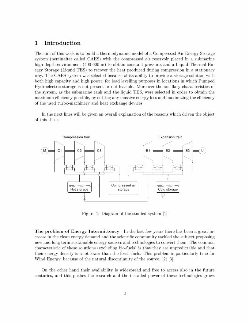
The aim of this work is to build a thermodynamic model of a Compressed Air Energy Storagesystem (hereinafter called CAES) with the compressed air reservoir placed in a submarinehigh depth environment (400-600 m) to obtain constant pressure, and a Liquid Thermal En-ergy Storage (Liquid TES) to recover the heat produced during compression in a stationaryway. The CAES system was selected because of its ability to provide a storage solution withboth high capacity and high power, for load levelling purposes in locations in which PumpedHydroelectric storage is not present or not feasible. Moreover the ancillary characteristics ofthe system, as the submarine tank and the liquid TES, were selected in order to obtain themaximum efficiency possible, by cutting any massive energy loss and maximizing the efficiencyof the used turbo-machinery and heat exchange devices.

In the next lines will be given an overall explanation of the reasons which driven the objectof this thesis.

Figure 1: Diagram of the studied system [1]

The problem of Energy Intermittency In the last few years there has been a great in-crease in the clean energy demand and the scientific community tackled the subject proposingnew and long term sustainable energy sources and technologies to convert them. The commoncharacteristic of these solutions (excluding bio-fuels) is that they are unpredictable and thattheir energy density is a lot lower than the fossil fuels. This problem is particularly true forWind Energy, because of the natural discontinuity of the source. [2] [3]

On the other hand their availability is widespread and free to access also in the futurecenturies, and this pushes the research and the installed power of these technologies grows

3

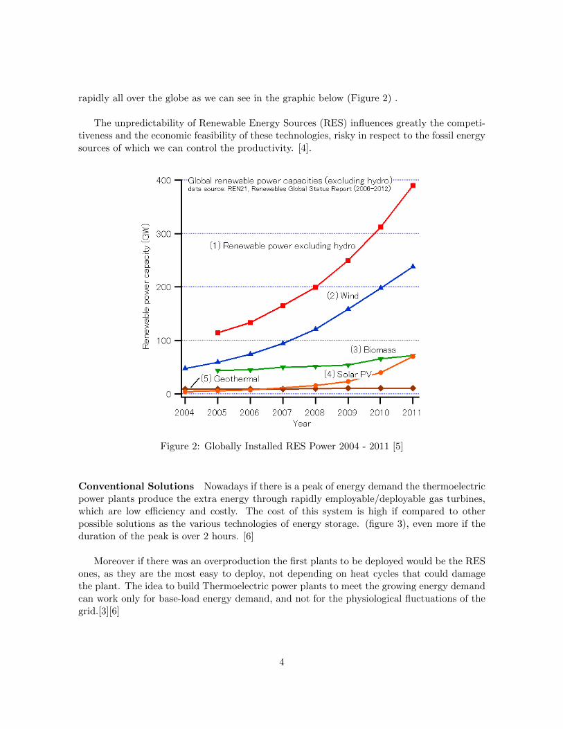
rapidly all over the globe as we can see in the graphic below (Figure 2) .

The unpredictability of Renewable Energy Sources (RES) influences greatly the competi-tiveness and the economic feasibility of these technologies, risky in respect to the fossil energysources of which we can control the productivity. [4].

Figure 2: Globally Installed RES Power 2004 - 2011 [5]

Conventional Solutions Nowadays if there is a peak of energy demand the thermoelectricpower plants produce the extra energy through rapidly employable/deployable gas turbines,which are low efficiency and costly. The cost of this system is high if compared to otherpossible solutions as the various technologies of energy storage. (figure 3), even more if theduration of the peak is over 2 hours. [6]

Moreover if there was an overproduction the first plants to be deployed would be the RESones, as they are the most easy to deploy, not depending on heat cycles that could damagethe plant. The idea to build Thermoelectric power plants to meet the growing energy demandcan work only for base-load energy demand, and not for the physiological fluctuations of thegrid.[3][6]

4

Figure 3: An EPRI economical feasibility study [7]

Energy Storage The alternative solution to the problem is storing part of the energy whenthere is low demand, and later recovering the stored energy when there is high demand. Nowthere are many storage options, that tackle particular storing needs. They can be sorted inthree categories, based on the order of magnitude of the time period the energy needs to bestored. These categories are:

• Load Levelling : Half day long fluctuations

• Ramping : Hour long fluctuations

• Frequency Regulation : Minute long fluctuations

In the figure 4 are showed the main storage systems that can deal with every single cate-gory.

Middle to small scale storage The most used and studied technologies for middleto small scale storage are batteries (middle scale) and flywheels (small scale). Flywheels areextremely efficient and have an extremely rapid response, but are also costly so they are usedonly for small scale. Recently other systems for small scale storage are being studied, such assuper-capacitors and SMES (Super Magnetic Energy Storage) that have also almost unitaryefficiencies, but are even more costly right now.

5

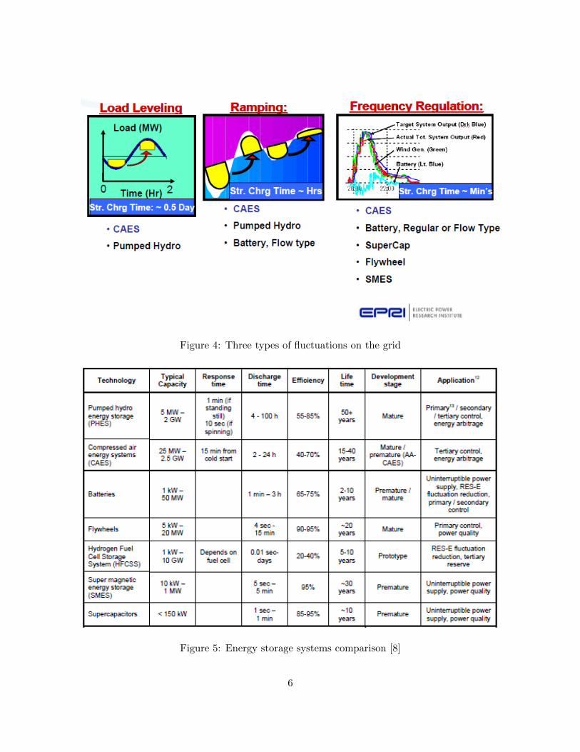
Figure 4: Three types of fluctuations on the grid

Figure 5: Energy storage systems comparison [8]

6

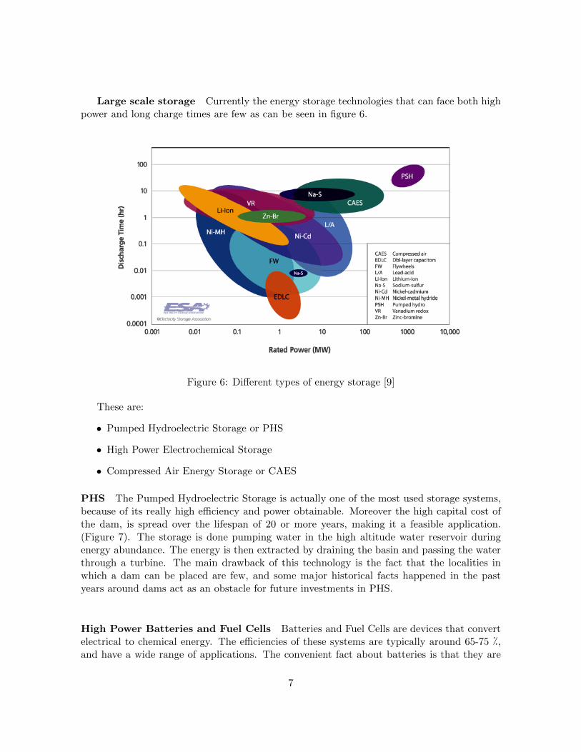
Large scale storage Currently the energy storage technologies that can face both highpower and long charge times are few as can be seen in figure 6.

Figure 6: Different types of energy storage [9]

These are:

• Pumped Hydroelectric Storage or PHS

• High Power Electrochemical Storage

• Compressed Air Energy Storage or CAES

PHS The Pumped Hydroelectric Storage is actually one of the most used storage systems,because of its really high efficiency and power obtainable. Moreover the high capital cost ofthe dam, is spread over the lifespan of 20 or more years, making it a feasible application.(Figure 7). The storage is done pumping water in the high altitude water reservoir duringenergy abundance. The energy is then extracted by draining the basin and passing the waterthrough a turbine. The main drawback of this technology is the fact that the localities inwhich a dam can be placed are few, and some major historical facts happened in the pastyears around dams act as an obstacle for future investments in PHS.

High Power Batteries and Fuel Cells Batteries and Fuel Cells are devices that convertelectrical to chemical energy. The efficiencies of these systems are typically around 65-75 �,and have a wide range of applications. The convenient fact about batteries is that they are

7

almost totally independent from geographical conditions, so can be placed in a large varietyof places. The drawbacks of these systems are the possible environmental hazards,the costand mostly the short lifespan. Lately EPRI analysed the economic feasibility of small scaleCAES systems that could be competitive with batteries. [10].

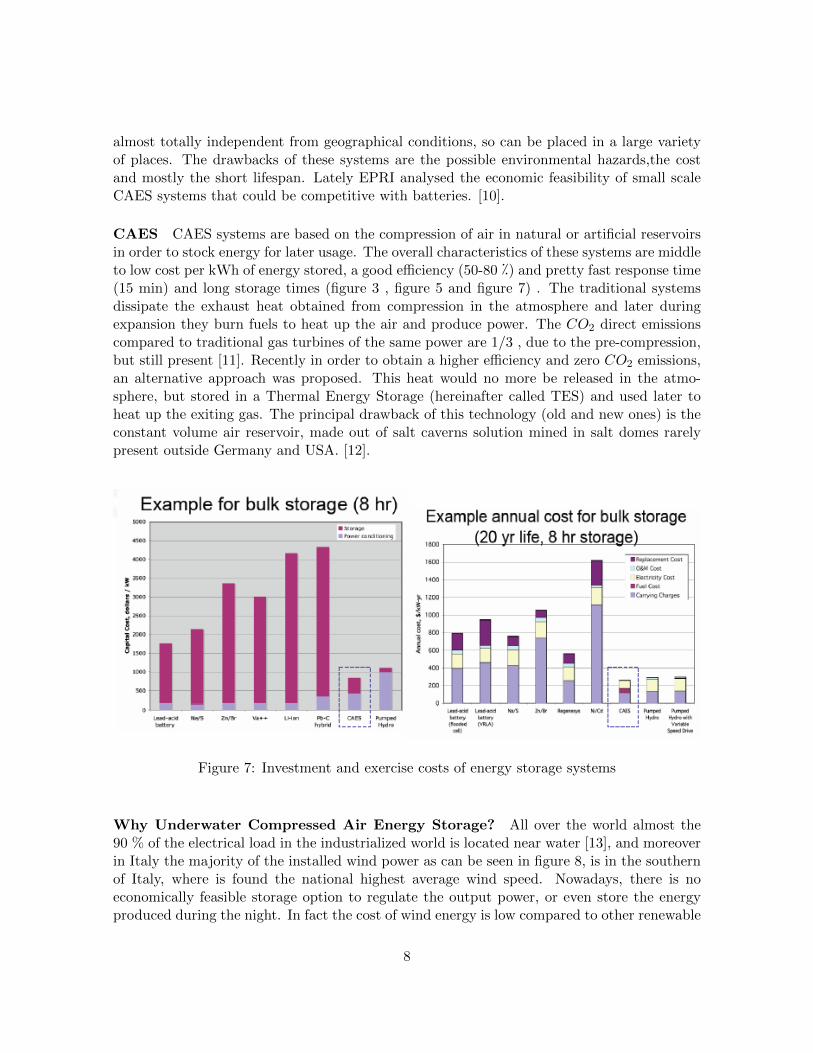
CAES CAES systems are based on the compression of air in natural or artificial reservoirsin order to stock energy for later usage. The overall characteristics of these systems are middleto low cost per kWh of energy stored, a good efficiency (50-80 �) and pretty fast response time(15 min) and long storage times (figure 3 , figure 5 and figure 7) . The traditional systemsdissipate the exhaust heat obtained from compression in the atmosphere and later duringexpansion they burn fuels to heat up the air and produce power. The CO2 direct emissionscompared to traditional gas turbines of the same power are 1/3 , due to the pre-compression,but still present [11]. Recently in order to obtain a higher efficiency and zero CO2 emissions,an alternative approach was proposed. This heat would no more be released in the atmo-sphere, but stored in a Thermal Energy Storage (hereinafter called TES) and used later toheat up the exiting gas. The principal drawback of this technology (old and new ones) is theconstant volume air reservoir, made out of salt caverns solution mined in salt domes rarelypresent outside Germany and USA. [12].

Figure 7: Investment and exercise costs of energy storage systems

Why Underwater Compressed Air Energy Storage? All over the world almost the90 % of the electrical load in the industrialized world is located near water [13], and moreoverin Italy the majority of the installed wind power as can be seen in figure 8, is in the southernof Italy, where is found the national highest average wind speed. Nowadays, there is noeconomically feasible storage option to regulate the output power, or even store the energyproduced during the night. In fact the cost of wind energy is low compared to other renewable

8

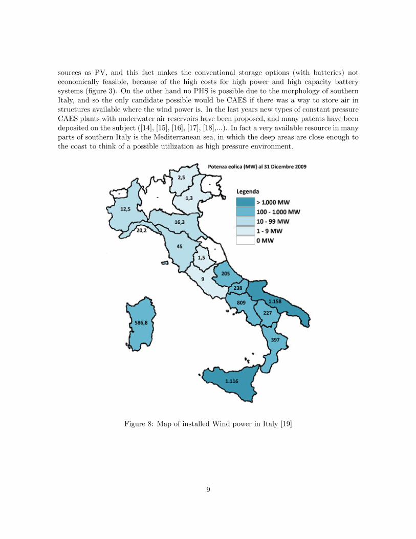
sources as PV, and this fact makes the conventional storage options (with batteries) noteconomically feasible, because of the high costs for high power and high capacity batterysystems (figure 3). On the other hand no PHS is possible due to the morphology of southernItaly, and so the only candidate possible would be CAES if there was a way to store air instructures available where the wind power is. In the last years new types of constant pressureCAES plants with underwater air reservoirs have been proposed, and many patents have beendeposited on the subject ([14], [15], [16], [17], [18],...). In fact a very available resource in manyparts of southern Italy is the Mediterranean sea, in which the deep areas are close enough tothe coast to think of a possible utilization as high pressure environment.

Figure 8: Map of installed Wind power in Italy [19]

9

2 CAES Classification

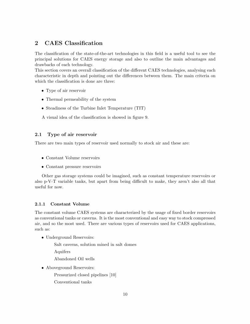
The classification of the state-of-the-art technologies in this field is a useful tool to see theprincipal solutions for CAES energy storage and also to outline the main advantages anddrawbacks of each technology.This section covers an overall classification of the different CAES technologies, analysing eachcharacteristic in depth and pointing out the differences between them. The main criteria onwhich the classification is done are three:

• Type of air reservoir

• Thermal permeability of the system

• Steadiness of the Turbine Inlet Temperature (TIT)

A visual idea of the classification is showed in figure 9.

2.1 Type of air reservoir

There are two main types of reservoir used normally to stock air and these are:

• Constant Volume reservoirs

• Constant pressure reservoirs

Other gas storage systems could be imagined, such as constant temperature reservoirs oralso p-V-T variable tanks, but apart from being difficult to make, they aren’t also all thatuseful for now.

2.1.1 Constant Volume

The constant volume CAES systems are characterized by the usage of fixed border reservoirsas conventional tanks or caverns. It is the most conventional and easy way to stock compressedair, and so the most used. There are various types of reservoirs used for CAES applications,such as:

• Underground Reservoirs:

Salt caverns, solution mined in salt domes

Aquifers

Abandoned Oil wells

• Aboveground Reservoirs:

Pressurized closed pipelines [10]

Conventional tanks

10

Figure 9: CAES Classification Criteria

Advantages This type of reservoir is actually the only one used in the industrial practice.The reason of this fact resides in a few characteristics of the system:

• Low cost per m3 for big volumes [10]

• High availability in northern Europe and USA [7].

• Well known technology

This type of storage uses a well known know-how inspired by the Natural Gas storage formarket purposes, a much older market with years of testing.

11

Disadvantages Unfortunately the constant volume storage has numerous disadvantagesthat have been brought up in these years of industrial practice at Huntorf (Germany) [20]and McIntosh (USA) [21], such as:

• Variable working points of turbomachineryConstant volume imposes variable pressures in the tank and makes the machines workin different points of their performance diagram, creating difficulties to optimize themachinery for the maximum efficiency. In the practice of the McIntosh plant the problemwas solved using a particular valve that maintains constant the inlet and outlet pressure,but that dissipates some energy, and costs a lot [21]. Other proposed solutions forthis problem were the usage of variable configuration compression/expansion trains orcompensating the variability of the pressure by changing the volume flow rate, in orderto maintain constant the working point of the turbomachinery.[22]

• Stresses in the reservoirVariable pressures create variable stress conditions in the cavern, that undergoes pulsat-ing fatigue cycles, reducing its viable lifespan. These fatigue cycles have been broughtunder control in the practice by reducing the amplitude of the cycle, and so reducingthe interval of variability of the pressure (under 20 bar) [12]. Other solutions to thisproblem have been proposed, such as increasing greatly the storage volume in order toreduce the pressure variability.

• Inefficient use of the storage volume As can be seen in figure 10, the ideal specific work(if the transformation was perfectly isothermal) varies greatly with the pressure makinga part of the air volume contained in the reservoir unusable, because of the low energydensity associated to the low pressures when the storage is discharged. Even if thereservoir was able to bear the stress cycles, the quality of the energy stored would godown greatly.

• Geographic localization (Only for underground storage)As with Hydroelectric water reservoirs , these underground caverns need some typicalGeomorphological conditions that permit the storage. Even if in Germany and northernEurope there is a relatively high number of usable sites [23], in Italy [12]the number isreally low. There is also no guarantee that the place where a reservoir possible, has thenecessary infrastructures or need for energy regulations and storage. In the past thisfact increased the capital cost for the plant, as reported here [24, p. 83] and here [21,p. 19].

• Air Vitiation (Only underground storage) [25]During the permanence of the air in the caverns a part of the oxygen contained inthe air becomes adsorbed into the rock or salt reducing the molar fraction of oxygenfrom 20,7 % to more or less 18 %.This fact is important to consider in the design of adiabatic/traditional CAES system because it can affect combustion efficiency.

12

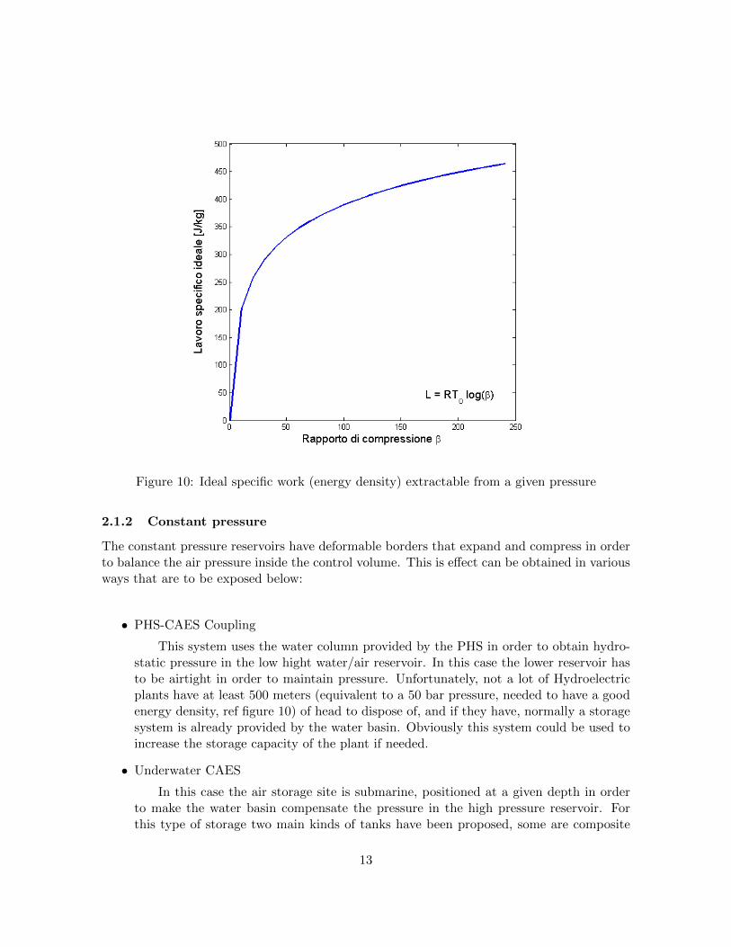
Figure 10: Ideal specific work (energy density) extractable from a given pressure

2.1.2 Constant pressure

The constant pressure reservoirs have deformable borders that expand and compress in orderto balance the air pressure inside the control volume. This is effect can be obtained in variousways that are to be exposed below:

• PHS-CAES Coupling

This system uses the water column provided by the PHS in order to obtain hydro-static pressure in the low hight water/air reservoir. In this case the lower reservoir hasto be airtight in order to maintain pressure. Unfortunately, not a lot of Hydroelectricplants have at least 500 meters (equivalent to a 50 bar pressure, needed to have a goodenergy density, ref figure 10) of head to dispose of, and if they have, normally a storagesystem is already provided by the water basin. Obviously this system could be used toincrease the storage capacity of the plant if needed.

• Underwater CAES

In this case the air storage site is submarine, positioned at a given depth in orderto make the water basin compensate the pressure in the high pressure reservoir. Forthis type of storage two main kinds of tanks have been proposed, some are composite

13

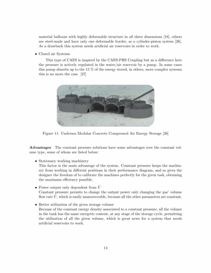
material balloons with highly deformable structure in all three dimensions [18], othersare steel-made and have only one deformable border, as a cylinder-piston system [26].As a drawback this system needs artificial air reservoirs in order to work.

• Closed air Systems

This type of CAES is inspired by the CAES-PHS Coupling but as a difference herethe pressure is actively regulated in the water/air reservoir by a pump. In some casesthis pump absorbs up to the 15 % of the energy stored, in others, more complex systemsthis is no more the case. [27]

Figure 11: Undersea Modular Concrete Compressed Air Energy Storage [26]

Advantages The constant pressure solutions have some advantages over the constant vol-ume type, some of whom are listed below:

• Stationary working machineryThis factor is the main advantage of the system. Constant pressure keeps the machin-ery from working in different positions in their performance diagram, and so gives thedesigner the freedom of to calibrate the machines perfectly for the given task, obtainingthe maximum efficiency possible.

• Power output only dependent from VConstant pressure permits to change the output power only changing the gas’ volumeflow rate V , which is easily manoeuvrable, because all the other parameters are constant.

• Better utilization of the given storage volumeBecause of the constant energy density associated to a constant pressure, all the volumein the tank has the same energetic content, at any stage of the storage cycle, permittingthe utilization of all the given volume, which is great news for a system that needsartificial reservoirs to work.

14

Disadvantages This type of storage solves many of the problems listed above for the con-stant volume reservoir, but also creates some extra difficulties to address such as:

• Possible piping installation difficultiesThe conditions under which constant pressure storages are possible are often not so easyto create or reach, so the installation could be difficult.

• Possible plant complexitiesThe constant pressure conditions aren’t easily reachable, so the plant complexity couldbe increased, as the underwater tanks could need either underwater piping or off shoreturbomachinery , and the other solutions may need pumps or PHS-CAES coupling.

• Possibly increased corrosive environment (salt)

2.2 Thermal permeability of the system

The thermal permeability of the system influences directly the overall efficiency of the CAES,contributing to limit or increase the internal losses.

We can distinguish two main permeability states:

• Diathermic SystemDiathermic means ”permeable to heat”, so this is a system that is designed to exchangeheat with the environment during all the cycle.

• Adiathermic SystemAdiathermic on the other hand means ”not permeable to heat”, in fact this type ofsystem is ideally designed to keep all the possible energy in the control volume, lettingescape only unavoidable losses.

2.2.1 Diathermic CAES

Diathermic types, are the only CAES systems that have a real plant working on the market(Huntorf and McIntosh). The diabatic CAES produces during compression a notably bigquantity of heat that is extracted from the gas through heat exchanges and is released inthe atmosphere, this is done because it reduces the amount of work needed for compression,reducing the costs. During expansion some fuel is burned in modified gas turbines (McIntosh)[21] or modified steam turbines (Huntorf)[12] in order to increase the overall power and keepthe ice from forming in the turbine. These systems have demonstrated great reliability andover 95/98 % availability in these years of non stop work [28]. Nevertheless the practice ofdispersing heat reduces the overall efficiency of the plant, in these cases around 50 %, producesCO2 and NOx emissions and creates the dependence of the exercise cost on fossil fuels costs.

15

2.2.2 Adiathermic CAES

Recently some systems have been proposed that store the heat produced during compressionin TES systems and use it during expansion in order to increase the efficiency of the plantsand to cut on polluting emissions. Theoretically, two approaches to the system can be pur-sued, but also one that combines the two, these are:

• Adiabatic approach

• Isothermal approach

• Combined approach

Adiabatic approach In the adiabatic approach, studied in a EU funded research, the ten-dency is to obtain the unitary efficiency through a perfectly adiabatic/isoentropic process.So the ideal plant would be one single machine that compresses air isoentropically and after-wards releases the produced (really high quality) thermal power into a TES. When the energyis needed, the air is heated up by the TES and expanded in a single isoentropical turbine.Sadly this approach has some technological limits, not for the efficiency of the turbines, thatare almost adiabatic, but because of the temperature and pressure jump problems, a 50 barcompression for a single machine are really difficult to bear, and produce a temperature jumpof 600-700 Celsius degrees also. These problems impose an inter-refrigerated compression inorder to reduce the mechanical and thermal stresses. [29]

Isothermal approach The ideal transformation for this approach is a perfectly isothermalone. The idea is to keep the gas temperature fixed during the compression and expansionobtaining this way the unitary efficiency. Nonetheless no machine fast enough to producereasonable amounts of power can do this, even if recently some companies have begun tostudy reciprocating compressors with almost isothermal compression curves, but with alsoless power and low efficiency compared to conventional turbomachinery [1]. For high powerapplications, as intended in this thesis, the alternative would be to approximate an isothermaltransformation with many inter-refrigerated compressions and inter-heated expansions . Inthis case the tendency is to obtain the unitary efficiency increasing the number of machines(the opposite way of the last approach) because this makes the transformation more similarto the isothermal one.

The advantages of this approach are that the maximum temperature the gas reaches isn’ttoo high, and this could permit the use of pressurized water as a cooling solution, which wouldpermit an open refrigerating cycle, versus a closed one. The advantage of this fact is thatgiven the prospected location if the plant (coastline or floating platform) and the presumableamounts of water needed, the use of water could be much more economic. Moreover, lowergas temperatures mean lower TES temperatures, and so less thermal losses.

16

The main drawback of this approach are the fact that in order to obtain η = 1 the numberof machines needed would be infinite, and so impossible. Moreover the marginal increase ofefficiency while increasing the machines would progressively lower as we approach 1 [30]. Thecosts of this practice impose a compromise as it was for the adiabatic approach.

Combined Approach Because of the fact that both the approaches ideally aren’t feasible,a compromise approach must be pursued. In this case, both the approaches need para-isothermal transformations as an approximation, and so a possible solution could be to find theperfect number of machines to obtain the best efficiency possible, in realistic conditions, andso also involving in the choice other plant parameters as the efficiency of the heat exchangersand the boundary conditions.

2.3 Stationariness of Turbine Inlet Temperature

The variability of the temperature of the TIT (Turbine Inlet Temperature) affects the station-ariness of the flow as greatly as the pressure variability does, so in relation to this parameterbig differences in CAES systems can come up.

Variable temperature at the border of elementary machines as turbines and compressorsis something that doesn’t happen often in real applications as the technology on which CAESturbines are based was designed for fuel applications, so temperature constancy is given bycontrolling the fuel intake. However for ecological and economical reasons the use of fuels isunwanted or has to be limited, so in these conditions, the only alternative is thermal storagewhich can cause in some cases the variability of the temperature.

2.3.1 Constant Temperature

This condition of the system is obtained in two very different ways:

• Fuel BurningAs the gas that is extracted from the reservoir enters the burner the temperature of thegas is regulated by the amount of fuel burned, in order to maintain constant the turbineinlet temperature.

• Liquid TESThe liquid thermal energy storages are systems which store heat in a fluid and the fluidin a tank. When needed the fluid is then extracted bit by bit, and only the temperatureof the extracted fluid is lowered, so that the temperature of the TES is maintainedconstant. In this way every cycle of the system will have the same TES temperatureand so the same TIT (turbine inlet temperature).

17

Advantages The main reasons why this condition is wanted are:

• Stationariness of the flowsThe temperature of a gas flow influences its volume flow rate, changing also the workingpoint of the machines. For this reason a steady flow is better.

• Simpler modelThe steadiness of the flow permits to simplify the numerical model, focussing of makingit more adherent from other points of view.

Disadvantages The disadvantages of constant pressure itself are none, in fact the draw-backs are linked only to the way this condition is reached.

Each way to maintain the temperature constant has its problems, so I will divide thedisadvantages accordingly to the technology that has it.

Fuel Burning

• Possible polluting emissionsIf the TIT is maintained constant burning fuels, the system will produce at least CO2

and NOx which are environmentally polluting compounds that in recent times have tobe limited.

• Fuel Cost DependenceThe exercise costs of the plant will be dependent on the cost of the burned fuel. In lastyears this cost reached unthinkable thresholds making less and less feasible a fuel basedstorage also because the tendency of fuel cost is to grow even more.

Liquid TES

• CostsThe costs of TES structures are high due to the cost of heat exchange devices and theirmaintenance. This drawback is shared between all the TES systems, not only the liquidtype, even if this particular type may be more complex due to the doubling of the heatexchange structures.

• Limited Storage TemperaturesDue to the usage of a fluid to exchange heat, the upper and lower extreme of thetemperature of the fluid are respectively the boiling and the fusion temperatures, becausein each case, the fluid ceases to be liquid. For this reason this storage type is difficult todesign, mainly because the fluids that work at low temperature boil if heated too much,and the ones that work at low temperature solidify if let cool down.

18

2.3.2 Variable Temperature

As said before, the variability of the temperature isn’t often found, but the usage of SensibleHeat Thermal Storages, makes is a possible horizon.

Advantages

• Large Storage temperature rangeThe sensible heat TES devices, opposed to the liquid TES types, have a large rangeof operating temperatures, because they normally use ceramic materials, like concrete,SiO2 sand, basalt, and so on. These materials have really high fusion temperatures, sothey can bear really wide ranges of working temperatures.

• Less costlyCompared to the liquid TES type, the cost of sensible heat devices can be lower due tothe lower complexity of the piping structure and of the materials used.

Disadvantages

• Modelling difficultiesBecause of the fact that in sensible heat devices the main body of the storage deviceis also the heat exchanger, the efficiency of the exchange and the gas exit temperaturevary with the temperature of the TES, making it quite difficult to model a system usingthis technology, conventional tools.

• Unsteadiness of the flow

19

Part I

Hydrostatic problem

In this part of the thesis a little analysis of the physical principles involving the mechanismthat maintains constant the pressure in a underwater CAES system will be done briefly. Someapproximations of reality, will be introduced and motivated.

3 Hydrostatic Hypothesis

The high pressure reservoir of the system is located on the bottom of the sea, at a high depth.I make here a simplifying hypothesis, in order to reduce the complexity of the given problem.Hereafter I’ll consider constant the pressure at the border of our control volume. This meansthat the possible changes in the level of the sea due to tides, waves, and the dynamic effectsof deep sea currents are to be considered negligible. This hypothesis is valid if we consider asite with low speed currents and at high depth, in order to make little the tidal and wavescontribution to pressure. Moreover, the system will be almost surely placed close to the seabed, where adherence conditions impose low speed currents if present. The possible differencesbetween the pressure between the top and the bottom of the reservoir border, are negligibleand will be hereafter ignored.

4 Full deformability of the air reservoir borders Hypothesis

Hereafter the tank borders will be considered fully deformable, this means that no load can besustained by it. This assumption can be considered valid in static conditions for free movingpiston-cylinder air vessels, and for highly deformable air balloons made of some polymer typematerial.

4.1 Hydrostatic Pressure

In hydrostatic conditions the pressure varies linearly with the depth of the site. The formulafor the pressure in these conditions is:

P = ρgz

where:

• ρ is the fluid density

• g is the earth’s gravitational constant

• z is the depth in meters (m)

This means that an air volume with deformable borders, placed at a certain depth is sub-jected to a given pressure that doesn’t change in time. Given the constant pressure outside

20

the control volume, because of the full deformability of the tank, no load can be sustained,and so the pressure inside the tank will be equal to the one outside.

Given the equality of internal and external pressure, the material of the air reservoir willnot be strained by any type of tensile stress caused by the pressure, the only component ofa possible tensile stress, comes from the buoyancy of the air volume and must be consideredwhile dimensioning the tank and the anchoring system.

4.2 Buoyancy

The force that the sunk air bubble feels and transfers to the air reservoir is given by thefollowing formula:

F = ρfgV

Where:

• ρ is the density of the fluid

• g is the earth’s gravitational constant

• V is the volume of the air bubble

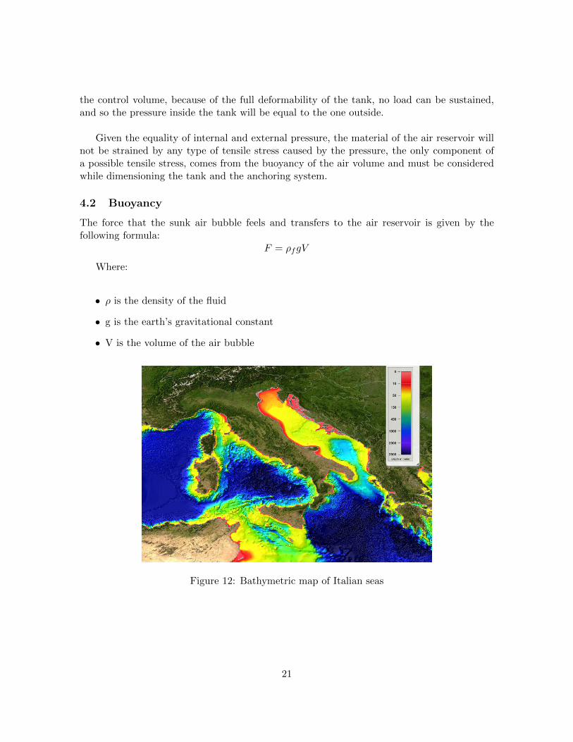
Figure 12: Bathymetric map of Italian seas

21

5 Geomorphological considerations

Study of the depth of the Italian seas The seas surrounding Italy are particular as canbe seen in the bathymetric chart (figure 12). The western part of the Mediterranean sea isparticularly deep close enough to the coast, in the range of 10 km in some places a depthof 500 m can be easily reached. This characteristic is useful to reduce the installation costsof the piping to connect the air reservoir to the system and limit the transport head losses.Moreover all over the Mediterranean there are places with the right depth even at longerdistances, for these a floating plant may be used. The principal usefulness of this morphologyis that the majority of the Italian wind farms are installed in southern Italy, a place wherethere are possibly the conditions to store energy through underwater CAES, but not mountainwater reservoirs for PHS, which is the only competitor for both high power and high capacityapplications at a reasonable cost.

22

Part II

Plant problem

6 Selection of the plant type

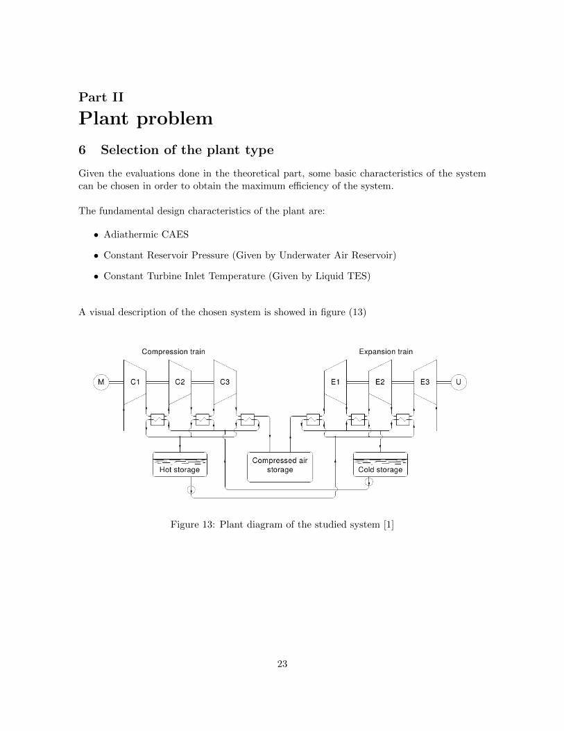
Given the evaluations done in the theoretical part, some basic characteristics of the systemcan be chosen in order to obtain the maximum efficiency of the system.

The fundamental design characteristics of the plant are:

• Adiathermic CAES

• Constant Reservoir Pressure (Given by Underwater Air Reservoir)

• Constant Turbine Inlet Temperature (Given by Liquid TES)

A visual description of the chosen system is showed in figure (13)

Figure 13: Plant diagram of the studied system [1]

23

7 Building the model

In this part the introductory notions listed before will be used to create a model of the chosensystem in order to produce later a numerical simulation of the system in order to optimize itand dimension some ancillary parts.

7.1 Gas model choice

The gas processed in this system, will be studied up to a pressure of 100 bar, the high pressuresinvolved make the ideal gas model normally used questionable, so in this section there will bea little analysis of the various models:

Ideal gas model The ideal gas model is quite simple, it permits a straight forward analysisof the transformations involving the gas. The analytical expression of this model is:

Pv = RT

Real Gas Model Real gases don’t completely agree with the conventional gas equations,in fact in particular pressure and temperature statuses they behave differently.In order toexpress this a coefficient known as Compressibility Factor ”Z” was introduced to correct thestandard formula:

Pv = ZRT

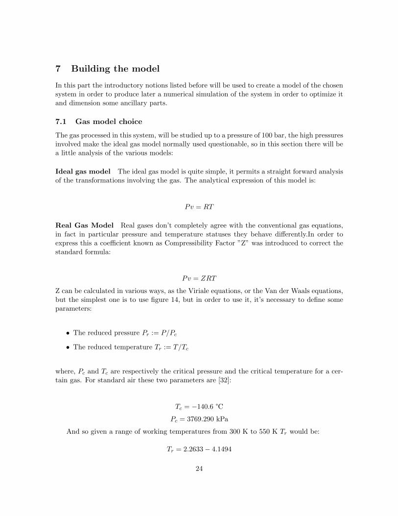
Z can be calculated in various ways, as the Viriale equations, or the Van der Waals equations,but the simplest one is to use figure 14, but in order to use it, it’s necessary to define someparameters:

• The reduced pressure Pr := P/Pc

• The reduced temperature Tr := T/Tc

where, Pc and Tc are respectively the critical pressure and the critical temperature for a cer-tain gas. For standard air these two parameters are [32]:

Tc = −140.6 °C

Pc = 3769.290 kPa

And so given a range of working temperatures from 300 K to 550 K Tr would be:

Tr = 2.2633− 4.1494

24

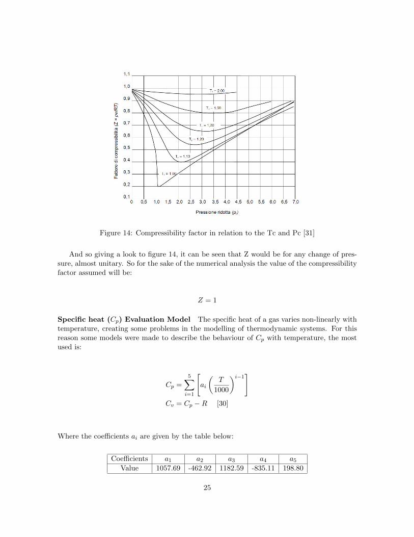
Figure 14: Compressibility factor in relation to the Tc and Pc [31]

And so giving a look to figure 14, it can be seen that Z would be for any change of pres-sure, almost unitary. So for the sake of the numerical analysis the value of the compressibilityfactor assumed will be:

Z = 1

Specific heat (Cp) Evaluation Model The specific heat of a gas varies non-linearly withtemperature, creating some problems in the modelling of thermodynamic systems. For thisreason some models were made to describe the behaviour of Cp with temperature, the mostused is:

Cp =

5∑i=1

[ai

(T

1000

)i−1]

Cv = Cp −R [30]

Where the coefficients ai are given by the table below:

Coefficients a1 a2 a3 a4 a5Value 1057.69 -462.92 1182.59 -835.11 198.80

25

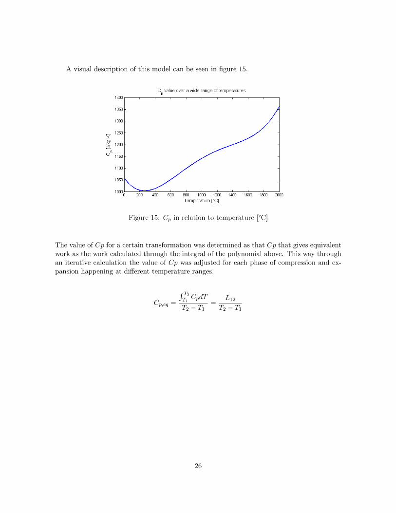
A visual description of this model can be seen in figure 15.

Figure 15: Cp in relation to temperature [°C]

The value of Cp for a certain transformation was determined as that Cp that gives equivalentwork as the work calculated through the integral of the polynomial above. This way throughan iterative calculation the value of Cp was adjusted for each phase of compression and ex-pansion happening at different temperature ranges.

Cp,eq =

∫ T2T1CpdT

T2 − T1=

L12

T2 − T1

26

7.2 Gas transformation model choice

This section will cover briefly adherent models found in literature about gas transformations.

7.2.1 Politropic transformation

The politropic transformation is the equivalent reversible transformation associated to what-soever gas transformation, even if irreversible. This model makes possible the evaluation ofreal gas transformations in which the irreversibility has to be taken into account. The basicformula of the politropic transformation is here reported:

Pvm = cost (7.1)

where m is known as the politropic index, and in normal transformations may vary from 0 to+∞. This transformation becomes the traditional isoentropic transformation when:

m = k = Cp/Cv

If compression and expansion were perfectly isoentropic, then the efficiency of the turboma-chinery would be 1 and we could obtain the best performance for the elementary machines.

7.2.2 Isothermal transformation

A word must be said also about isothermal transformation, because the maximum efficiency ofthe system could be obtained also through a perfectly isothermal compression and expansion.This because the energy consumed and released would be identical. This said, a perfectlyisothermal transformation for gases is quite difficult to obtain, because typical compressorsand expansors are almost adiabatic. This is why an approximation of it, called para-isothermaltransformation is often done.

7.2.3 Para-Isothermal transformation

The para-isothermal transformation is a combination of politropic and isobaric transforma-tions, in order to obtain an almost isothermal transformation. The concept of an ideal para-isothermal transformation is showed in the figure 16.

Ideal para-isothermal transformation The ideal transformation is obtained by alter-nating real turbomachines and ideal heat exchangers that are simply thought to ideally bringback the temperature to the same level phase after phase of the compression or expansion. Adetailed description of the phenomena was found here [30]. Because of the fact that no realheat exchanger can do this an alternative model must be chosen.

Real para-isothermal transformation The analytical model described before , was takenas a basis for the production of a much more adherent model counting also the non-idealheat exchangers used in a real case . In fact the graph showed above shows compression(red) and expansion (green) transformations that are always brought back to the ambient

27

Figure 16: Thermodynamic paraisothermal cycle with ideal heat exchange

temperature by the ideal heat exchangers. This doesn’t happen in reality, and the cyclewould have slightly increasing CIT’s (compressor inlet temperature) and slightly decreasingTIT’s (turbine inlet temperature).This fact is a main complexity that imposed a numericalapproach to the problem, and reduces (greatly, as will be showed later) the efficiency of thestorage system.

7.3 Continuous and localised pressure losses

Any gas flowing in pipelines produces pressure losses. In the piping system and in the heatexchangers some energy is lost in the form of heat, directly lowering the pressure of the gas.In the examined case, the pressure losses will be expressed as suggested here: [33, p. 35]:

∆P

ρ=

(fL

D+ ζ

)c2

2(7.2)

7.3.1 Piping pressure losses

This type of losses happens after the compression and before the expansion, so during com-pression, we obtain a lower pressure in the reservoir, and during expansion we obtain a lowerturbine inlet pressure. These are continuous pressure losses that can be evaluated as follows:

∆P

ρ=

(fpLpDp

)c2p2

These losses are directly linked to the length of the piping, so an evaluation of the lengthin relation to the depth of the reservoir and distance from the coast is necessary.

28

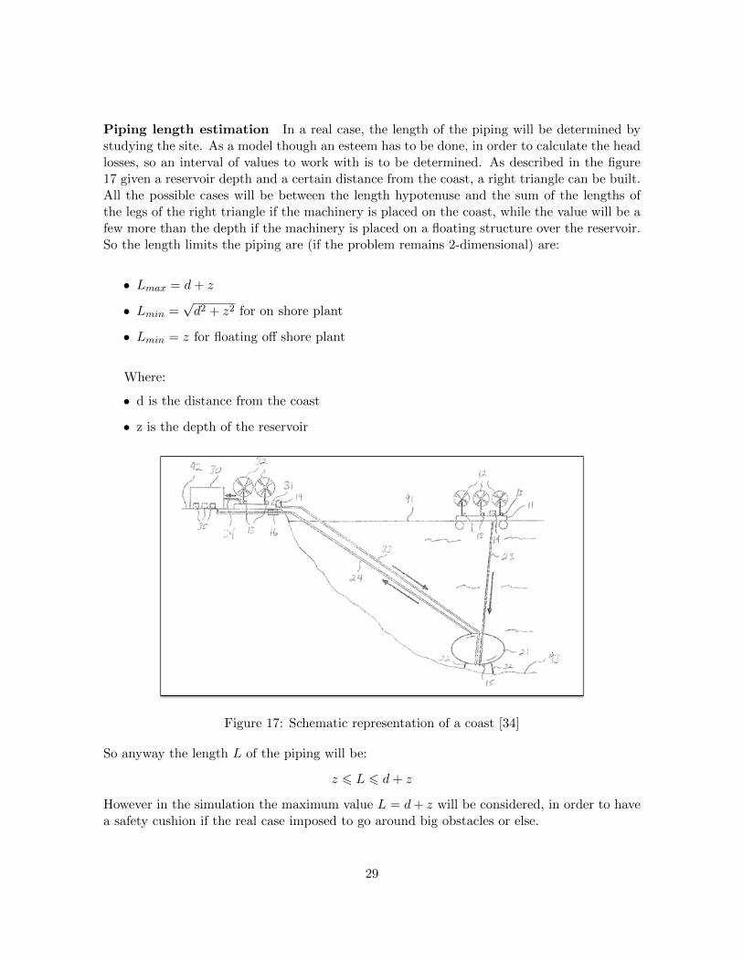
Piping length estimation In a real case, the length of the piping will be determined bystudying the site. As a model though an esteem has to be done, in order to calculate the headlosses, so an interval of values to work with is to be determined. As described in the figure17 given a reservoir depth and a certain distance from the coast, a right triangle can be built.All the possible cases will be between the length hypotenuse and the sum of the lengths ofthe legs of the right triangle if the machinery is placed on the coast, while the value will be afew more than the depth if the machinery is placed on a floating structure over the reservoir.So the length limits the piping are (if the problem remains 2-dimensional) are:

• Lmax = d+ z

• Lmin =√d2 + z2 for on shore plant

• Lmin = z for floating off shore plant

Where:

• d is the distance from the coast

• z is the depth of the reservoir

Figure 17: Schematic representation of a coast [34]

So anyway the length L of the piping will be:

z 6 L 6 d+ z

However in the simulation the maximum value L = d+ z will be considered, in order to havea safety cushion if the real case imposed to go around big obstacles or else.

29

7.3.2 Local pressure losses

The localized pressure losses in the plant are not simple to predict, except for few cases:

• Reservoir Inlet/Outlet pressure losses

• Diameter variations of the pipe (Turbine/Compressor connections)

• Heat exchangers

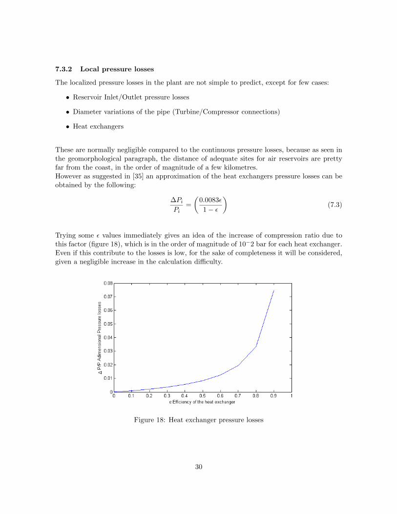
These are normally negligible compared to the continuous pressure losses, because as seen inthe geomorphological paragraph, the distance of adequate sites for air reservoirs are prettyfar from the coast, in the order of magnitude of a few kilometres.However as suggested in [35] an approximation of the heat exchangers pressure losses can beobtained by the following:

∆PiPi

=

(0.0083ε

1− ε

)(7.3)

Trying some ε values immediately gives an idea of the increase of compression ratio due tothis factor (figure 18), which is in the order of magnitude of 10−2 bar for each heat exchanger.Even if this contribute to the losses is low, for the sake of completeness it will be considered,given a negligible increase in the calculation difficulty.

Figure 18: Heat exchanger pressure losses

30

7.3.3 Compression

Let’s demonstrate how the pressure losses affect the compression ratio β:

βnew =P2,new

P1=P2,new − P2 + P2

P1=

∆P + P2

P1

βnew = β +∆P

P1(7.4)

Where:

• βnew is the new compression ratio after the losses.

• P2,new is the new COP (compressor outlet pressure) after the losses.

• P2, P1 are respectively the reservoir pressure and the ambient pressure.

Given that eq. (7.4) is also valid for every stage:

βnew,i = βi +∆PiPi

(7.5)

Nonetheless this equation is valid:

βi = β1Nc (7.6)

So combining the equations (7.5),(7.4) and (7.6) we obtain:

βc,i = Nc

√(βid +

∆PpipPpip

)+

∆PHEPHE

Where (pip) is the piping component and (HE) is the heat exchanger component. A similarequation can be obtained for expansion, as showed in the following section.

31

8 Numerical Approach to the problem

Because of the complexity of the chosen model, an analytical approach brought to even morecomplexity, where a numerical approach based on few formulas simplified greatly the problem.

8.1 Optimization function

In order to analyse the CAES, an optimization function of the system was defined, based onsix important parameters. The function is the efficiency of the overall system.

η = f(β, V , Cr, ε, TOT,Nc

)The parameters on which the efficiency depends are:

• β, the compression ratio

• V the volume flow rate

• Cr the heat capacity ratio between gas and refrigerant

• ε, the efficiency of the heat exchangers

• TOT, the Turbine Outlet Temperature

• Nc the number of compression phases

These where chosen because of either are controllable flow parameters, as β and V , or plantdesign fundamental parameters, as ε, Nc and TOT. Moreover TOT was chosen for exampleover Ne, the number of expansion phases, because of external limits imposed on TOT, moreeasily complied this way.

32

8.2 Constraints

In order to comply to all the possible mechanical, thermodynamic and economical restrictionsimposed by real conditions, some constraints were imposed to the optimization function. Theconstraints are the following:

• TOT ≥ 5 °CThis condition was due to avoiding the icing in the last stages of the expansion turbine.In fact because of the non-fuel burning choice, the temperatures in the turbine couldlower below 0 °C causing the formation of ice on the blades, and so lowering also theefficiency and the lifespan of the machine.

• Qe ≤ QcBecause of the structure of the numerical simulation, the compliance to the first law ofthermodynamics wasn’t assured. This condition imposes that the heat absorbed by theturbine has to be less or equal to the heat produced by the compression.

• Nc, Ne ≥ 2 This is a pre-constraint about the selection of the machines. No machine candeal alone with both the pressure and temperature jump needed for a CAES system.So this case is excluded , in order to avoid obtaining the efficiency associated to theadiabatic approach, that would probably be very high, and totally independent from ε.

Now the formulas used in the model will be showed and explained briefly.

9 Equations on which the model is based

9.1 Elementary Compression Ratio

As discussed before, the compression ratio a single machine has to produce is influenced by thelosses, so the real compression ratio of each i-th machine is given from the following formulas:

Compression

βc,i = Nc

√(βid +

∆PpipPpip

)+

∆PHEPHE

Expansion

βe,i = Ne

√(βid −

∆PpipPpip

)− ∆PHE

PHE

33

Where:

• βid is the ideal compression ratio, the one we want to obtain between the reservoirpressure and the ambient pressure.

•∆PpipPpip

are the piping pressure losses.

• Nc and Ne are the number of compression and expansion phases

•∆PHEPHE

are the Heat exchanger pressure losses

9.2 Specific Work of the single phase

In order to evaluate the efficiency and the power output of the system, an expression of thespecific work is needed:

Compression

Lc,i = Cp,gasTi (βνci − 1)

The overall work consumed will be:

Lc =

Nc∑i=1

Lc,i

Expansion

Le,i = Cp,gasTe,i(1− β−νei

)The overall work produced will be:

Le =

Ne∑i=1

Le,i

9.3 Efficiency

The overall efficiency of the system is defined as the ratio between the outgoing energy flowsand the ingoing energy flows. For this particular system will be:

η :=LeLc

34

9.4 Power

The power produced by the system is simply given by the following formula:

P := mLe

where m is the mass flow rate evolving in the system.

9.5 Definition of heat exchange efficiency

A lot of the following equations are based on this definition simple formula of efficiency ofan heat exchanger. The efficiency is the ratio between Qre, the heat actually exchanged, andQmax the maximum heat possibly exchangeable by the heat exchanger.

ε :=QreQmax

(9.1)

Now let’s define Qre and Qmax in order to use this equation.

9.6 Real Exchanged Heat

The heat exchanged really between the refrigerant and the gas can be seen from two pointsof view, the gas and the refrigerant points of view, so here are the formulas that describe both:

Compression

Qre =mgasCp,gas (Ti−1βνci − Ti)

=mrefCp,ref (TAC,i − TAF )

35

Where:

• Ti is the i-th Compressor Inlet Temperature (CIT), the T1 temperature coincides withthe ambient temperature Tamb

• TAF and TAC,i are respectively the cold refrigerant (constant during compression) andthe i-th hot refrigerant temperature (each heat exchanger gives off the refrigerant at adifferent temperature).

Expansion

Qre,e =mgasCp,gas (Te,i − Tue,i−1)

=mrefCp,ref (TAC − TAF,i)

Where:

• Te,i is the i-th turbine inlet temperature (TIT).

• Tue,i is the i-th turbine outlet temperature (TOT).

9.7 Maximum Exchangeable Heat

The maximum exchangeable heat is defined as the heat exchanged between the larger possibletemperature difference and seen by the minimum Cp point of view. It’s given by the followingformulas [33]:

Compression

Qmax = mminCp,min (Ti−1βνci − TAF )

Expansion

Qmax,e =mminCp,min (TAC − Tue,i−1)

36

9.8 Temperatures of the fluids

In order to comply to the previously imposed constraints, and to better analyse the system, agood overview of the temperatures reached in all the parts of the plant is beneficial. To obtainthe following equation, was done a combination, of the definition of heat exchange efficiency,Qre and Qmax.

Gas Compressor Inlet Temperature (CIT) The following equation expresses the tem-perature of the gas when it enters the compressor in each i-th phase.

Ti = Ti−1βνci − ε

mminCp,minmgasCp,gas

(Ti−1βνci − TAF )

where T1 = Tamb

If the minimum mCp is the gas one (min=gas), then:

Ti = Ti−1βνci − ε (Ti−1β

νci − TAF )

If the minimum mCp is the refrigerant one (min=ref), then:

Ti = Ti−1βνci −

ε

Cr(Ti−1β

νci − TAF )

Where, we define Cr, the heat capacity ratio:

Cr =mgasCp,gasmrefCp,ref

Refrigerant Heat Exchanger Outlet Temperature This is the temperature that therefrigerant fluid has once exited the i-th heat exchange device, and so right before going tothe hot TES.

TAC,i = TAF + εmminCp,minmrefCp,ref

(Ti−1βνci − TAF )

with TAF = cost

37

if min=gas,then:

TAC,i = TAF + εCr (Ti−1βνci − TAF )

If min=ref, then:

TAC,i = TAF + ε (Ti−1βνci − TAF )

Hot TES Temperature The hot TES temperature is only the mean temperature of allthe temperatures of the fluids exiting the heat exchangers, this because they mix togetheronce introduced in the TES, and because they have all the same mass flow rate:

TAF =

Nc∑i=1

TAC,i

Nc

Gas Turbine Outlet Temperature (TOT) This is the temperature the gas has afterbeing expanded by the i-th turbine phase:

Tue,i = β−νci

(Tue,i−1 + ε

mminCp,minmgasCp,gas

(TAC − Tue,i−1)

)If min=gas, then:

Tue,i = β−νci (Tue,i−1 + ε (TAC − Tue,i−1))

If min=ref, then:

Tue,i = β−νci

(Tue,i−1 +

ε

Cr(TAC − Tue,i−1)

)

38

Gas Turbine Inlet Temperature (TIT) This is the temperature the gas has a momentbefore entering the turbine (the first TIT is the reservoir one, and we assume that has thesame temperature of the sea):

Te,i = Tue,i−1 + εmminCp,minmgasCp,gas

(TAC − Tue,i−1)

If min=gas, then:

Te,i = Tue,i−1 + ε (TAC − Tue,i−1)

If min=ref, then:

Te,i = Tue,i−1 +ε

Cr(TAC − Tue,i−1)

Warming Fluid Heat Exchanger Outlet Temperature This is the temperature of thefluid coming from the hot TES (here called Warming fluid) after being cooled down by theheat exchanger that is warming up the gas:

TAF,i = TAC + εmminCp,minmrefCp,ref

(Tue,i − TAC)

where TAC = cost

If min=gas, then:

TAF,i = TAC + εCr (Tue,i − TAC)

If min=ref, then:

TAF,i = TAC + ε (Tue,i − TAC)

39

10 Results

Using the above equations, a numerical simulation was run. An iterative routine had to beimplemented in order to consider the head losses.

Boundary Conditions The following data was assumed during the simulation:

• Ambient Temperature Tamb = 295K

• Air Reservoir Temperature Tserb = 285K

• Cold Refrigerant Temperature TAF = 289K

• Politropic efficiency of the machinery ηpol = 0.9

• Piping Diameter D = 1 m

• Piping roughness rug = 5.5 10−5 m

10.1 Pre-Dimensioning of the Plant

A first series of routines were run to find the best operating parameters in order to reach themaximum efficiency.

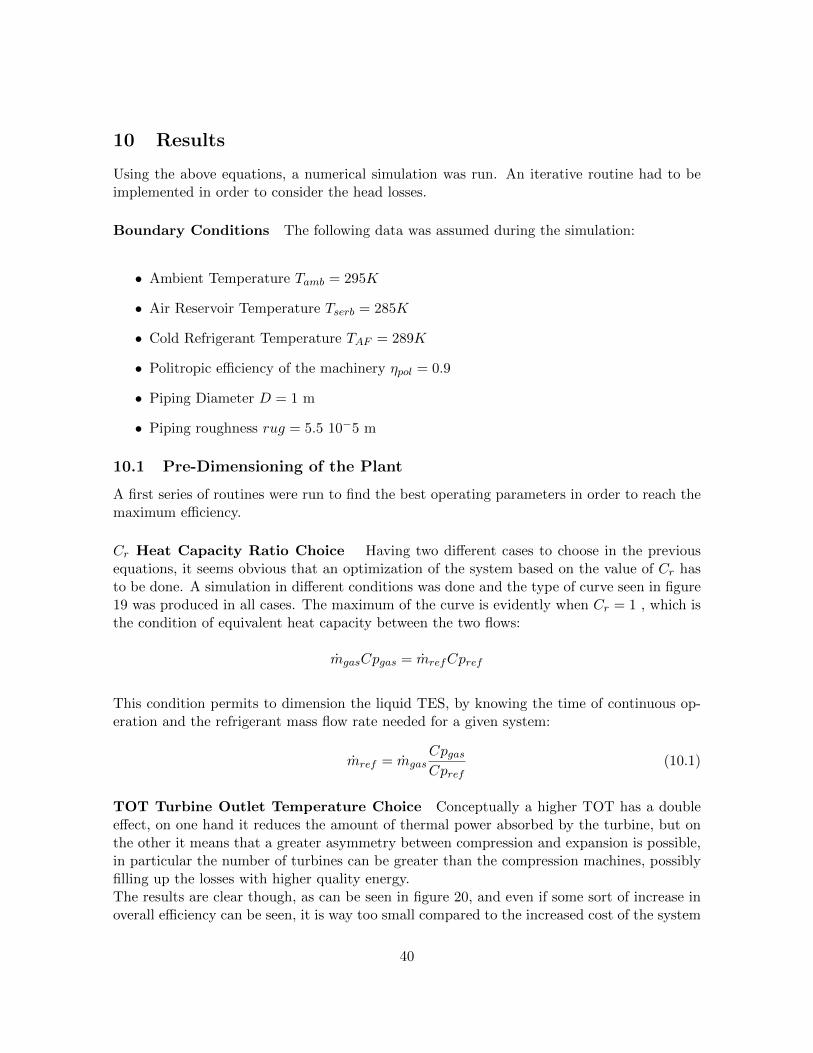
Cr Heat Capacity Ratio Choice Having two different cases to choose in the previousequations, it seems obvious that an optimization of the system based on the value of Cr hasto be done. A simulation in different conditions was done and the type of curve seen in figure19 was produced in all cases. The maximum of the curve is evidently when Cr = 1 , which isthe condition of equivalent heat capacity between the two flows:

mgasCpgas = mrefCpref

This condition permits to dimension the liquid TES, by knowing the time of continuous op-eration and the refrigerant mass flow rate needed for a given system:

mref = mgasCpgasCpref

(10.1)

TOT Turbine Outlet Temperature Choice Conceptually a higher TOT has a doubleeffect, on one hand it reduces the amount of thermal power absorbed by the turbine, but onthe other it means that a greater asymmetry between compression and expansion is possible,in particular the number of turbines can be greater than the compression machines, possiblyfilling up the losses with higher quality energy.The results are clear though, as can be seen in figure 20, and even if some sort of increase inoverall efficiency can be seen, it is way too small compared to the increased cost of the system

40

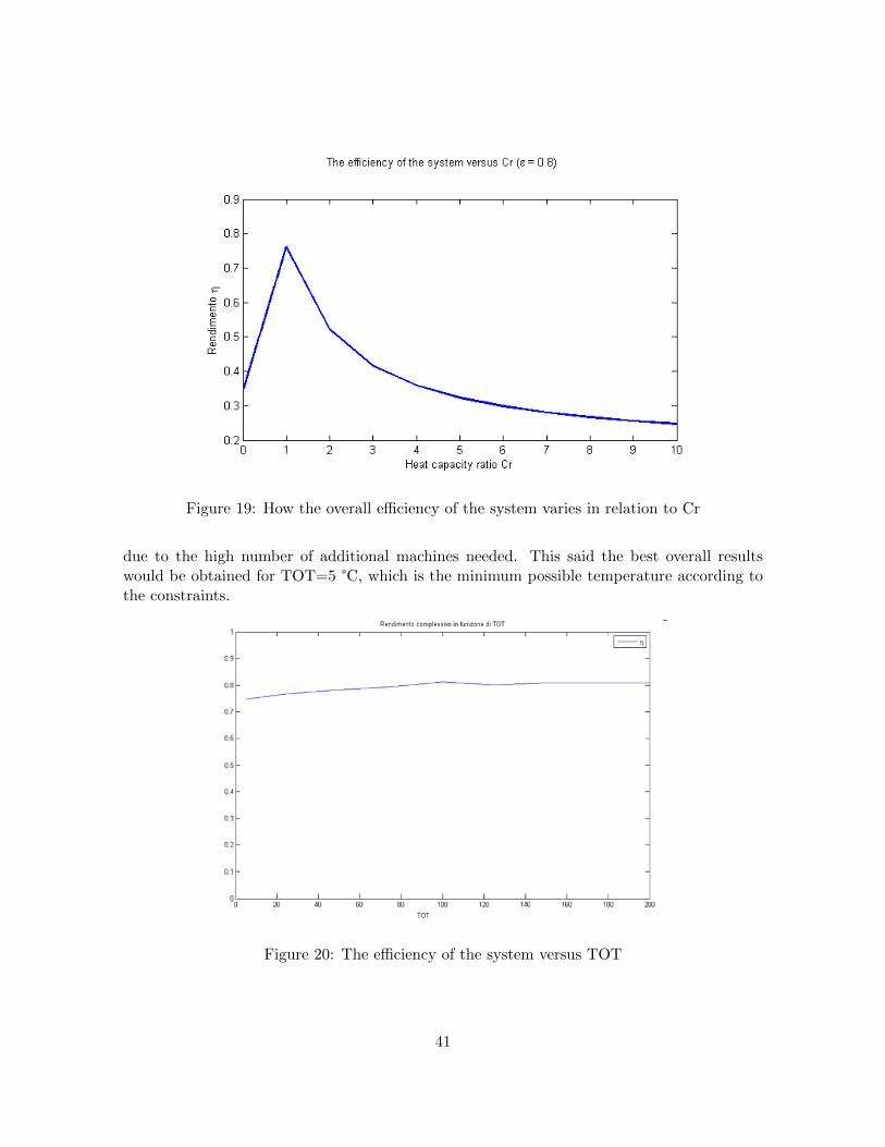
Figure 19: How the overall efficiency of the system varies in relation to Cr

due to the high number of additional machines needed. This said the best overall resultswould be obtained for TOT=5 °C, which is the minimum possible temperature according tothe constraints.

Figure 20: The efficiency of the system versus TOT

41

Nc Number of compression phases and ε the efficiency of heat exchange Thesetwo parameters are closely related, and influence the efficiency in a symbiotic way, for thisreason the results are showed together (figure 21). As can be seen, there is a tendency of the

Figure 21: The efficiency of the system in relation to both the heat exchange efficiency andthe number of compression phases

efficiency to be optimum for a high number of compression phases for low efficiency exchang-ers, while at higher efficiencies there are two different local maximums, one for low numbersof compression phases, the other for lower ones.

This data concludes the definition of the ”Combined Approach”, discussed before. The max-imum efficiency of the system, is more towards the ”isothermal approach” when we use lowefficiency heat exchangers, and more towards the adiabatic approach” when using high ef-ficiency heat exchangers. A possible motivation of this behaviour is that, the isothermalapproach imposes a higher number of heat exchangers, and so if the quality is low a highernumber of them gets better results, while if the quality is high a greater number is not neededin order to obtain high efficiencies, and as can be seen unless you increase the number a lot,it’s even worst because the inefficiencies due to the increased number of exchanges is notbalanced by the increased efficiency due to the isothermal approach. Certainly using veryhigh numbers of phases at high efficiencies of the heat exchangers is also possible, but morecostly.

The overall efficiency is almost linearly dependent from the heat exchange ef-ficiency Another fact showed in the table exposed before is the strong link between theoverall efficiency of the system η and the efficiency of the heat exchangers ε. As can be seenis figure 22, η is almost linearly dependent form ε and it does so for a wide range of values.This fact underlines that the main energy losses of the system now are the thermal losseshappening during the heat exchange and that the main focus of the optimization of this typeof plants has to be in the design of almost unitary efficiency heat exchangers.

42

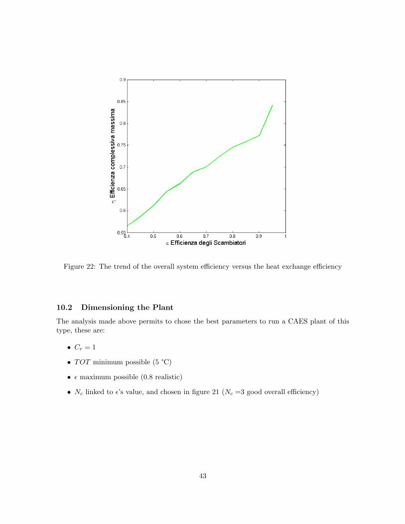
Figure 22: The trend of the overall system efficiency versus the heat exchange efficiency

10.2 Dimensioning the Plant

The analysis made above permits to chose the best parameters to run a CAES plant of thistype, these are:

• Cr = 1

• TOT minimum possible (5 °C)

• ε maximum possible (0.8 realistic)

• Nc linked to ε’s value, and chosen in figure 21 (Nc =3 good overall efficiency)

43

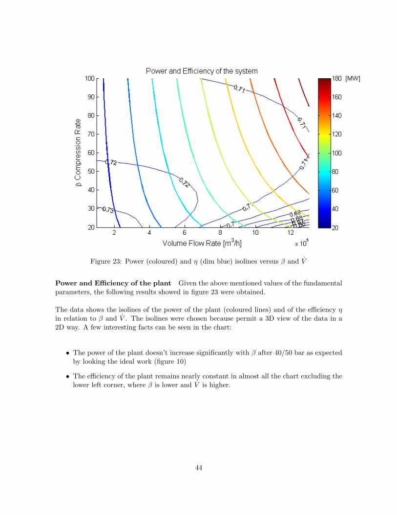
Figure 23: Power (coloured) and η (dim blue) isolines versus β and V

Power and Efficiency of the plant Given the above mentioned values of the fundamentalparameters, the following results showed in figure 23 were obtained.

The data shows the isolines of the power of the plant (coloured lines) and of the efficiency ηin relation to β and V . The isolines were chosen because permit a 3D view of the data in a2D way. A few interesting facts can be seen in the chart:

• The power of the plant doesn’t increase significantly with β after 40/50 bar as expectedby looking the ideal work (figure 10)

• The efficiency of the plant remains nearly constant in almost all the chart excluding thelower left corner, where β is lower and V is higher.

44

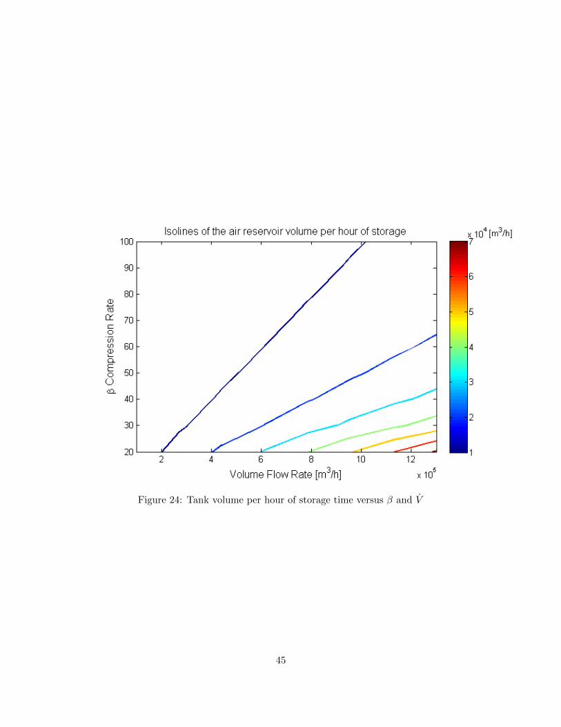
Figure 24: Tank volume per hour of storage time versus β and V

45

Volume of the air reservoir An important parameter for dimensioning the plant wouldbe the volume of the underwater air reservoir. Unfortunately it depends on three parameters:

Vtank = f(β, V , storagetime

)

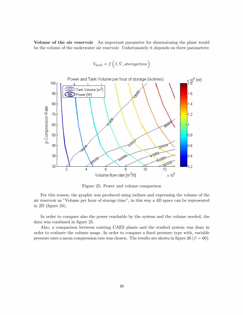
Figure 25: Power and volume comparison

For this reason, the graphic was produced using isolines and expressing the volume of theair reservoir as ”Volume per hour of storage time”, in this way a 4D space can be representedin 2D (figure 24).

In order to compare also the power reachable by the system and the volume needed, thedata was combined in figure 25.

Also, a comparison between existing CAES plants and the studied system was done inorder to evaluate the volume usage. In order to compare a fixed pressure type with, variablepressure ones a mean compression rate was chosen. The results are shown in figure 26 (β = 60).

46

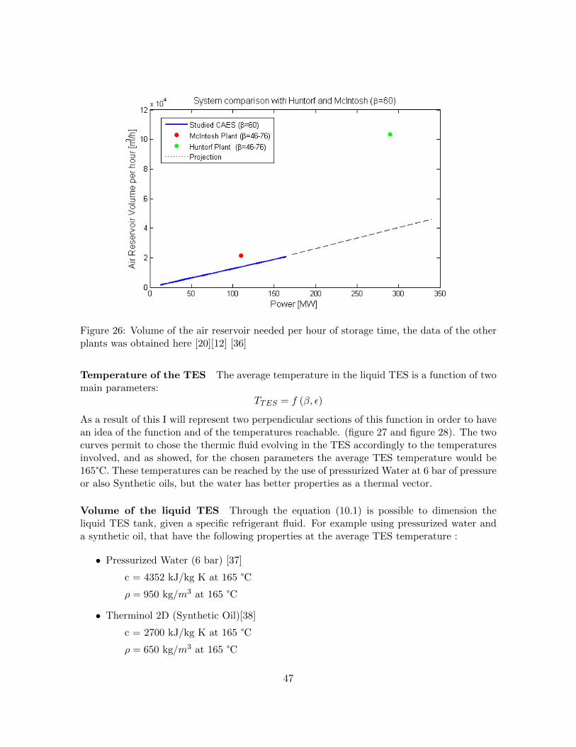
Figure 26: Volume of the air reservoir needed per hour of storage time, the data of the otherplants was obtained here [20][12] [36]

Temperature of the TES The average temperature in the liquid TES is a function of twomain parameters:

TTES = f (β, ε)

As a result of this I will represent two perpendicular sections of this function in order to havean idea of the function and of the temperatures reachable. (figure 27 and figure 28). The twocurves permit to chose the thermic fluid evolving in the TES accordingly to the temperaturesinvolved, and as showed, for the chosen parameters the average TES temperature would be165°C. These temperatures can be reached by the use of pressurized Water at 6 bar of pressureor also Synthetic oils, but the water has better properties as a thermal vector.

Volume of the liquid TES Through the equation (10.1) is possible to dimension theliquid TES tank, given a specific refrigerant fluid. For example using pressurized water anda synthetic oil, that have the following properties at the average TES temperature :

• Pressurized Water (6 bar) [37]

c = 4352 kJ/kg K at 165 °C

ρ = 950 kg/m3 at 165 °C

• Therminol 2D (Synthetic Oil)[38]

c = 2700 kJ/kg K at 165 °C

ρ = 650 kg/m3 at 165 °C

47

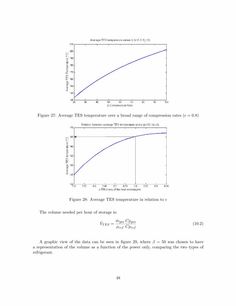
Figure 27: Average TES temperature over a broad range of compression rates (ε = 0.8)

Figure 28: Average TES temperature in relation to ε

The volume needed per hour of storage is:

VTES =mgas

ρref

CpgasCpref

(10.2)

A graphic view of the data can be seen in figure 29, where β = 50 was chosen to havea representation of the volume as a function of the power only, comparing the two types ofrefrigerant.

48

Figure 29: TES Volume needed per hour or storage using water or a specific synthetic oil asrefrigerant (β = 50)

11 Conclusions

As a result of the analysis the following statements were proven right:

• The studied system complies to both the power and the storage times reachable by aCAES system.(figure 6)

• The efficiency of this type of system is in the range of 60-80 %, as obtained by othersimilar studies [39]

• It isn’t convenient to increase the storage pressure over 40-50 bar, because the energydensity doesn’t increase sufficiently.

• The principal limit to the overall efficiency is the efficiency of the heat exchangers.

• Increasing the TOT, doesn’t increase significantly the efficiency

• For high heat exchange efficiencies the adiabatic approach is preferred, while the isother-mal approach is better for low efficiency exchangers.

• The storage volumes for the constant pressure CAES type can be considerably lowerthan the constant volume ones.

• The use of pressurized water requires considerably less TES volume compared to asynthetic oil.

49

References

[1] Giuseppe Grazzini and Adriano Milazzo. A thermodynamic analysis of multistage adia-batic caes. Proceedings of the IEEE, 100(2):461–472, 2012.

[2] Jeffery B. Greenblatt, Samir Succar, David C. Denkenberger, Robert H. Williams, andRobert H. Socolow. Baseload wind energy: modeling the competition between gas tur-bines and compressed air energy storage for supplemental generation. Energy Policy,35(3):14741492, 2007. URL http://www.sciencedirect.com/science/article/pii/

S0301421506001509.

[3] I. Arsie, V. Marano, G. Nappi, and G. Rizzo. A model of a hybrid power plant withwind turbines and compressed air energy storage. In Proc. of ASME Power Conference,Chicago, Illinois (USA), 2005. URL http://zanran_storage.s3.amazonaws.com/www.

dimec.unisa.it/ContentPages/16839477.pdf.

[4] I Arsie, V Marano, M Moran, G Rizzo, and G Savino. Optimal management of awind/caes power plant by means of neural network wind speed forecast. In Euro-pean Wind Energy Conference and Exhibition, The European Wind Energy Association(EWEA), Milan, May 7, volume 10, 2007.

[5] Wikipedia. Renewable energy. Wikipedia, 2010-2013. URL http://en.wikipedia.org/

wiki/Renewable_energy.

[6] Benjamin R Bollinger. System and method for rapid isothermal gas expansion andcompression for energy storage, August 2012. US Patent 8,240,146.

[7] EPRI. Epri caes demo to study design, performance, reliability and cost. Technicalreport, Electric Power Research Inst., Palo Alto, CA (United States); Alabama ElectricCooperative, Andalusia, AL (United States). CAES Plant, April 2009.

[8] Carl Zach, Hans Auer, and Lettner Georg. Report summarizing the current status, roleand costs of energy storage technologies. Technical report, Energy Economics Group(EEG), www.store-project.eu, mar 2012.

[9] Emanuele Bozzolani. Techno-economic analysis of compressed air energy storage systems.2010.

[10] EPRI. Epri updates cost projections for compressed air energy storage. Technical report,Electric Power Research Institute, August 2009.

[11] Dr. James Eliot Mason. Analysis of wind base load electricity generation in the u.s.Renewable Energy Research Institute, 2009.

[12] Enrico Benini. Thermodynamic analysis of Compressed Air Energy Storage systems. PhDthesis, Universita degli studi di Trento, 2011.

[13] Scott Raymond Frazier; Brian Von Herzen. Underwater compressed fluid energy storagesystem, 2011. US Patent App. 2011/0070032 A1.

50

[14] Poonum Agrawal, Ali Nourai, Larry Markel, Richard Fioravanti, Paul Gordon, NellieTong, and Georgianne Huff. Characterization and assessment of novel bulk storage tech-nologies. Sandia report SAND2011-3700, 2011.

[15] Emmanuel B Agamloh, Iqbal Husain, and Ali Safayet. Investigation of the electricalsystem design concept and grid connection of ocean energy devices to an offshore com-pressed energy storage system. In Energy Conversion Congress and Exposition (ECCE),2012 IEEE, pages 2819–2826. IEEE, 2012.

[16] Scott Raymond Frazier and Brian Von Herzen. Underwater compressed fluid energystorage system, March 2011. US Patent 20,110,070,032.

[17] JB Herbich and P Versowsky. Wave forces on underwater storage tanks. In Engineeringin the Ocean Environment, Ocean’74-IEEE International Conference on, pages 233–239.IEEE, 1974.

[18] Scott Raymond Frazier and Brian Von Herzen. System for underwater compressed fluidenergy storage and method for deploying same, 2011.

[19] APER. Report eolico italia. Technical report, 2010.

[20] Fritz Crotogino, Klaus-Uwe Mohmeyer, and Roland Scharf. Huntorf caes: Morethan 20 years of successful operation. Orlando, Florida, USA, 2001. URL http:

//www.uni-saarland.de/fak7/fze/AKE_Archiv/AKE2003H/AKE2003H_Vortraege/

AKE2003H03c_Crotogino_ea_HuntorfCAES_CompressedAirEnergyStorage.pdf.

[21] R Pollak. History of first us compressed air energy storage (caes) plant (110mw 26h)volume 2: Construction. Electric Power Research Institute, EPRI TR-101751, 1994.

[22] Giuseppe Grazzini and Adriano Milazzo. Thermodynamic analysis of caes/tes systemsfor renewable energy plants. Renewable Energy, 33(9):1998–2006, 2008.

[23] EPRI. Epri report analyzes caes plant reference design and costs. Technical report,Electric Power Research Institute, January 2012.

[24] JO Goodson. History of first us compressed air energy storage (caes) plant (110-mw-26 h). Technical report, Electric Power Research Inst., Palo Alto, CA (United States);Alabama Electric Cooperative, Andalusia, AL (United States). CAES Plant, 1992.

[25] EPRI. Reducing caes capital and operating costs. Technical report, Electric PowerResearch Inst., Palo Alto, CA (United States); Alabama Electric Cooperative, Andalusia,AL (United States). CAES Plant, April 2011.

[26] James Kesseli. Modular undersea compressed air energy storage (ucaes) system.Department of Energy Award, 2011. URL http://energy.gov/sites/prod/files/

ESS%202012%20Peer%20Review%20-%20Modular%20Undersea%20Compressed%20Air%

20Energy%20Storage%20(UCAES)%20System%20-%20James%20Kesseli,%20Brayton%

20Energy.pdf.

51

[27] Y.M. Kim, D.G. Shin, and D. Favrat. Operating characteristics of constant-pressurecompressed air energy storage (caes) system combined with pumped hydro storage basedon energy and exergy analysis. Energy, 36(10):6220 – 6233, 2011. ISSN 0360-5442. doi: 10.1016/j.energy.2011.07.040. URL http://www.sciencedirect.com/science/article/

pii/S0360544211004889.

[28] Dr. Robert B. Schainker. Compressed air energy storage (caes): Executive summary.Technical report, EPRI, aug 2010. URL http://disgen.epri.com/downloads/

EPRI%20CAES%20Demo%20Proj.Exec%20Overview.Deep%20Dive%20Slides.by%20R.

%20Schainker.Auguat%202010.pdf.

[29] Stefan Zunft, Christoph Jakiel, Martin Koller, and Chris Bullough. Adiabatic com-pressed air energy storage for the grid integration of wind power. In Sixth Interna-tional Workshop on Large-Scale Integration of Wind Power and Transmission Networksfor Offshore Windfarms, page 2628, 2006. URL http://elib-v3.dlr.de/46856/1/

OffshoreWS-Zunft060825final.pdf.

[30] Lorenzo Battisti. I Processi nelle Macchine a Fluido. Lorenzo Battisti Editore, 1 edition,October 2012.

[31] Compressibility factor wikipedia, . URL http://en.wikipedia.org/wiki/

Compressibility_factor.

[32] Critical temperatures and pressures of various substances, . URL http://www.

engineeringtoolbox.com/gas-critical-temperature-pressure-d_161.html.

[33] William M. Kays and A. L. London. Compact Heat Exchangers. McGraw-Hill, 3 edition,1984.

[34] Herbert L. Williams. Energy generation system using underwater storage of compressedair produced by wind machines, 2013. International Patent WO 2013/013027.

[35] Naser M. Jubeh and Yousef S.H. Najjar. Green solution for power generation by adoptionof adiabatic caes system. Applied Thermal Engineering, 44(0):85 – 89, 2012. ISSN 1359-4311. doi: 10.1016/j.applthermaleng.2012.04.005. URL http://www.sciencedirect.

com/science/article/pii/S1359431112002360.

[36] U.S.DOE. Technical and economic analysis of various power generation resources coupledwith caes systems. 2011.

[37] Celsius. Water thermodynamic properties, . URL http://www.celsius-process.com/

_en/tools.php.

[38] Celsius. Therminol 2d thermodynamic properties, . URL http://www.

celsius-process.com/_en/tools.php.

[39] Adriano Milazzo. Optimization of the configuration in a caes-tes system. 1st InternationalWorkshop ”Shape and Thermodynamics”, September 2008. URL http://eprints.bice.

rm.cnr.it/1378/.

52