Embed Size (px)
Citation preview

Compositional Scheduling AnalysisUsing Standard Event Models
The SymTA/S Approach
KAI RICHTER
Dissertation, 2005
Institute of Computer and Communication Network EngineeringDepartment of Electrical Engineering and Information TechnologyTechnical University Carolo-Wilhelmina of BraunschweigBraunschweig, Germany
Kai
Ric
hter
C
ompo
sitio
nal S
ched
ulin
g A
naly
sis
Usi
ng S
tand
ard
Even
t Mod
els


Compositional Scheduling Analysis
Using Standard Event Models
The SymTA/S Approach
KAI RICHTER
Dissertation, 2005
Institute of Computer and Communication Network Engineering
Department of Electrical Engineering and Information Technology
Technical University Carolo-Wilhelmina of Braunschweig
Braunschweig, Germany


Compositional Scheduling AnalysisUsing Standard Event Models
(Kompositionelle Schedulinganalysemit Standard-Ereignismodellen)
Von der Gemeinsamen Fakultat fur Maschinenbau und Elektrotechnikder Technischen Universitat Carolo-Wilhelmina zu Braunschweig
zur Erlangung der Wurde
eines Doktor-Ingenieurs (Dr.-Ing.)
genehmigte Dissertation
eingereicht am: 25. Oktober 2004
mundliche Prufung am: 22. Dezember 2004
von: Dipl.-Ing. Kai Robert Richter
aus: Northeim, Bundesrepublik Deutschland
Referent: Prof. Dr.-Ing. Rolf Ernst
Referent: Prof. Dr. Petru Eles
Vorsitzender: Prof. Dr. Jorn-Uwe Varchmin
2005

COMPOSITIONAL SCHEDULING ANALYSISUSING STANDARD EVENT MODELS
The SymTA/S Approach
KAI RICHTERInstitute of Computer and Communication Network EngineeringDepartment of Electrical Engineering and Information TechnologyTechnical University of BraunschweigBraunschweig, Germany

ii COMPOSITIONAL SCHEDULING ANALYSIS

Abstract
The ever increasing advances in silicon and communication technology al-low the integration of increasing functionality in digital embedded systems,ranging from mobile phones through multimedia home platforms to automo-tive control networks. Embedded system designers have to cope with this in-creasing system complexity whilst still building competitive systems to sur-vive the market pressure, thus requiring increasing productivity. Componentand sub-system specialization and re-use provide this productivity, but systemintegration is becoming a new bottleneck because the resulting heterogeneoussystem must be analyzed and verified. This thesis focuses on the performanceand timing verification aspect.
Many embedded systems are real-time systems and must meet a variety oftiming requirements, such as deadlines and limited load or bandwidth, underall possible corner-case operating conditions. But verification is difficult astiming properties depend heavily on interactions between tasks in the systemand on the scheduling of individual tasks and communications. Unfortunately,the current practice of specialization and re-use results in increasingly hetero-geneous systems, which specifically complicates the scheduling analysis prob-lem. Even today’s best practice of timed simulation is increasingly unreliable,mainly because the corner cases are extremely difficult to find and debug, andit is even more difficult to find simulation patterns to cover them all.
As an alternative, formal scheduling analysis techniques systematically ana-lyze corner cases and provide guaranteed bounds on certain timing properties.Many approaches have been proposed, but most of them are limited to sub-problems, such as a single operating system. They ignore the complex, hetero-geneous nature of today’s applications and architectures, and they cannot bereasonably combined because they use different underlying analysis models.Few approaches target more complex and heterogeneous systems and havetheir application in specific areas, such as network processor design. Theseapproaches, however, are often too unwieldy and complex to be accepted or

iv COMPOSITIONAL SCHEDULING ANALYSIS
understood by the embedded system industry. We summarize that none of theexisting techniques is sufficiently general to comprehensively cover arbitraryheterogeneous systems.
The main objective of this thesis is to develop a scheduling analysis pro-cedure that a) can cope with the increasing complexity and heterogeneity ofembedded systems, b) provides the modularity and flexibility that the estab-lished, re-use driven system integration style requires, and c) facilitates systemintegration using a comprehensible analytical model.
In this thesis, a novel, structured analysis model is presented, that elegantlycaptures the system-level component interactions using intuitive event models.These event models represent the interfaces between different components, andthe clear interface structure allows their efficient adaptation to different ana-lytical models. Several previously incompatible component and sub-systemanalysis techniques can now –for the first time– be heterogeneously combinedinto a system-level analysis. This allows the modular integration of heteroge-neous system parts, whilst providing designers with the flexibility to use theirpreferred local techniques without compromising global scheduling analysis.
Based on this structured analysis model, we define a sound analysis pro-cedure that consists of few comprehensible steps. The procedure is generalenough that it can also detect and solve subtle design pitfalls, such as schedul-ing anomalies or cyclic dependencies, which are virtually impossible to findusing simulation. The sound view on the component interactions substantiallyimproves designers’ understanding of the key integration problems, and allowsthem to influence and control these interactions to optimize the system glob-ally.
The application of the approach is demonstrated in detail using a variety ofexpressive examples and experiments. As the new analysis procedure can beefficiently applied in practice, it provides a serious and promising complementto simulation. It allows comprehensive system integration and optimization,and it provides much more reliable performance analysis results, at the sametime requiring far less computation time.

Kurzfassung
Als Folge des technologischen Fortschritts bei Halbleitern und Kommuni-kationsmedien werden heute zunehmend mehr Funktionen in digitalen, ein-gebetteten Systemen integriert. Beispiele reichen von relativ kleinen Mobil-telefonen uber Multi-Media Heimgerate bis hin zu vernetzter Automobilelek-tronik. Um konkurrenzfahige Produkte zu entwickeln muss die steigende Sys-temkomplexitat bewaltigt werden. Die dazu notwendige Entwurfsproduktivitatwird vermehrt durch die Wiederverwendung und Integration von spezialisier-ten Systemkomponenten (Hardware und Software) erreicht, was allerdings zuneuen Engpassen fuhrt, denn die Integration und das resultierende heterogeneGesamtsystem muss analysiert und verifiziert werden. Die vorliegende Arbeitbefasst sich mit Kernfragen der Performanz- und Echtzeitanalyse solcher Sys-teme.
Eingebettete Systeme sind zumeist Echtzeitsysteme und mussen eine Viel-zahl von Zeit- und Performanzanforderungen erfullen, z. B. maximale Reak-tionszeiten oder vorgegebene Kommunikationsbandbreiten, und zwar unter Be-achtung aller Randfalle (worst-case). Die Echtzeiteigenschaften hangen starkvom Zusammenspiel der Einzelkomponenten sowie deren Scheduling durchBetriebssysteme und Kommunikationsprotokolle ab. Unglucklicherweise fuhrtgerade die Wiederverwendung von spezialisierten Komponenten zu einer He-terogenitat, die die Schedulinganalyse zusatzlich erschwert. Als Folge sind dienach dem Stand der Technik eingesetzten Simulationsverfahren zusehends un-zuverlassig, da die kritischen Randfalle in der Praxis kaum mehr vollstandigbestimmt werden konnen.
Als Alternative zur Simulation zeichnen sich formale Methoden gerade beider Betrachtung von Randfallen durch ein systematisches und zuverlassigesVorgehen aus. Der Großteil existierender Ansatze ist jedoch auf spezielleTeilprobleme beschrankt, z. B. die isolierte Analyse eines Betriebssystems.Aufgrund der unterschiedlichen zugrundeliegenden Analysemodelle sind dieseAnsatze inkompatibel zueinander und eignen sich nicht zur Analyse heteroge-
vi COMPOSITIONAL SCHEDULING ANALYSIS
ner Systeme. Einige wenige Ansatze erfassen zwar komplexere Systeme ausspeziellen Anwendungsgebieten, z. B. Netzwerkprozessoren, sind jedoch furden Allgemeinfall zu unhandlich und finden daher nur eine geringe Akzep-tanz. Zusammenfassend stellen wir fest, dass es heute keine hinreichend all-gemeingultige Technik zur umfassenden Schedulinganalyse von heterogenenSystemen gibt.
Das Hauptziel dieser Arbeit ist die Entwicklung eines Verfahrens zur Sche-dulinganalyse, das a) die steigende Komplexitat und Heterogenitat angemes-sen erfasst, b) uber die Modularitat und Flexibilitat verfugt, die mit Wieder-verwendung und Integration erforderlich ist, und c) die Integration durch einnachvollziehbares Analysemodell unterstutzt.
Diese Arbeit stellt ein neues, strukturiertes Analysemodell vor, das die kom-plexen Abhangigkeiten auf der Systemebene mit Hilfe von intuitiven Ereignis-modellen erfasst. Diese Ereignismodelle bilden die Schnittstellen zwischenunterschiedlichen Komponenten, und die klare Strukturierung ermoglicht dieeffiziente Anpassung dieser Schnittstellen an verschiedenartige Analysemo-delle. Dadurch konnen nun erstmals mehrere unterschiedliche, vormals inkom-patible Teilsystemanalysen wiederverwendet und unter Beibehaltung der Sys-temstruktur heterogen zu einer Gesamtsystemanalyse zusammengesetzt wer-den (Komposition). Dies erlaubt die modulare Integration von unterschied-lichen Systemteilen und gibt Entwicklern gleichzeitig die notige Flexibilitat,ihre bevorzugten lokalen Entwurfsmethoden zu benutzen, ohne auf die globaleSchedulinganalyse verzichten zu mussen.
Das Analysemodell bildet die Grundlage fur ein allgemein anwendbaresAnalyseverfahren, das aus wenigen intuitiven Schritten besteht. Das Verfah-ren ermoglicht Entwicklern, auch diejenigen subtilen Performanzprobleme zuerkennen und aufzulosen, die beispielsweise durch Schedulinganomalien oderkomplexe zyklische Abhangigkeiten hervorgerufen werden und in der Simula-tion praktisch unerkannt bleiben. Durch die Darstellung der Komponentenin-teraktionen mittels verstandlicher Ereignismodelle konnen die Kernproblemeder Integration nachvollzogen werden. Weiterhin kann gezielt auf die Kom-ponenteninteraktion Einfluss genommen und das System global optimiert wer-den.
Das Verfahren und die Anwendung wird an einer Reihe aussagekraftigerBeispiele und Experimente im Detail erlautert. Es ist in der Praxis sehr ef-fizient einsetzbar, womit sich eine ernstzunehmende und vielversprechendeErganzung zur heute etablierten Performanz-Simulation eroffnet. Im Vergleichermoglicht das neue Verfahren eine umfassende Systemintegration und -opti-mierung und liefert zuverlassige Analyseergebnisse in deutlich kurzerer Zeit.

Acknowledgments
This thesis summarizes the key scientific results of my research at the In-stitute of Computer and Communication Network Engineering (IDA) at theTechnical University of Braunschweig, Germany.
First of all, I would like to express my sincere gratitude to my advisor Pro-fessor Rolf Ernst for introducing me to embedded real-time systems research,and for supporting me finding my way through. His visionary and challengingideas –in combination with his patience, insight, and guidance– made this the-sis possible and SymTA/S a successful project. I also want to thank ProfessorPetru Eles for his constructive comments related to my research and my dis-sertation, and for agreeing to co-examine this work, and Professor Jorn-UweVarchmin for chairing the examination committee.
I have had the pleasure to work together with a group of very talented,fun, and challenging people. Many thanks to Dirk Ziegenbein and Marek Jer-sak, my wonderful colleagues and friends in the SPI project. Marek againfor our fruitful ongoing collaboration in the SymTA/S project, and for shar-ing the boldness to turn it into an entrepreneurial partnership. I also want tothank my junior colleagues Jorn-Christian Braam, Arne Hamann, Rafik Henia,Ruben Jubeh, Razvan Racu, Simon Schliecker, and Jan Staschulat who en-riched the SymTA/S project both scientifically and personally. Thanks also toHans Gronniger and to all other contributors in the SPI and SymTA/S projects.
Further thanks go to the research groups of Professor Lothar Thiele in Zurichand Professor Jurgen Teich in Paderborn/Erlangen, especially to Simon Kunzliand Christian Haubelt, and to others for cooperations in many projects.
I want to thank the institute staff for providing and maintaining a profes-sional but still personal work environment, the labs for repeatedly helping merepairing my bike and electronic gadgets, Prof. Ernst again for funding theinstitute’s fully-automatic high-end espresso machine, and Gwylim Jones forproof-reading the manuscript.

viii COMPOSITIONAL SCHEDULING ANALYSIS
I want to thank my parents for recognizing and intensifying my scientific-technical interests early, and for encouraging me to study engineering. Mostimportantly, I want to thank my beloved and charming Alexandra for her sup-port and understanding for the effort it took me writing up this thesis, for herpatience when I was coming home late or working in the week-ends, and forthe love and the joy we share in our personal life.
Finally, I like to thank all people who expected to be honored explicitly here.This line is dedicated to you!

Contents
List of Figures xvList of Tables xix
1 INTRODUCTION 11.1 Influences on HW/SW System Performance 31.2 Performance Simulation and Coverage 61.3 Objectives & Outline 8
2 SCHEDULING AND PERFORMANCE ANALYSIS 112.1 Component Scheduling Analysis 11
2.1.1 Rate-Monotonic Scheduling 122.1.2 Other Static-Priority Schedulers 142.1.3 Dynamic Priority Assignments 172.1.4 Time-Driven Scheduling 182.1.5 Other Scheduling Strategies 192.1.6 Industrial Application 19
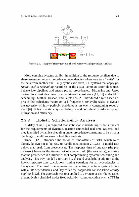
2.2 System-Level Extensions 202.2.1 Homogeneous Multi-Processors 202.2.2 Holistic Schedulability Analysis 21
2.3 Flow-Based Analysis 232.3.1 Event Vectors 232.3.2 Arrival Curves 24
2.4 Previous Own Work 252.5 Summary & New Approach 25
2.5.1 Evaluation 252.5.2 Revised Objectives & Basic Idea 272.5.3 Key Challenges 27

x COMPOSITIONAL SCHEDULING ANALYSIS
2.5.4 Detailed Outline 29
3 INPUT EVENT MODELS 313.1 Task Activation and Event Streams 313.2 Common Properties of Event Streams 323.3 Strictly Periodic Events 33
3.3.1 The η(∆t) Functions 333.3.2 The δ(n) Functions 37
3.4 Event Streams vs. Event Models 383.5 Periodic Events with Jitter 39
3.5.1 The η(∆t) Functions 393.5.2 The δ(n) Functions 423.5.3 Event Model Definition 43
3.6 Sporadic Events 443.6.1 The η(∆t) Functions 443.6.2 The δ(n) Functions 453.6.3 Event Model Definition 46
3.7 Sporadically Periodic Events 463.7.1 The η(∆t) Functions 463.7.2 The δ(n) Functions 483.7.3 Event Model Definition 49
3.8 Summary 49
4 OUTPUT EVENT MODELS 514.1 Periodic Task Activation 51
4.1.1 Constant Response Times 524.1.2 Response Time Intervals and Output Jitter 524.1.3 Inheritance of Input Jitter 534.1.4 Event Streams with Large Jitters 55
4.2 Implications of Large Jitters 574.2.1 Propagation of Large Jitters 584.2.2 Limitations and Inefficiencies 604.2.3 Modeling Alternatives 61
4.3 A New Model: Periodic Events with Burst 624.3.1 The η(∆t) Functions 634.3.2 The δ(n) Functions 644.3.3 Bounding the Minimum Output Distance 65
4.4 Sporadic Task Activation 65

Contents xi
4.4.1 Constant Response Time 664.4.2 Response Time Interval 664.4.3 Decreasing Inter-Arrival Times 674.4.4 Sporadically Periodic Task Activation 67
4.5 Conditional Output Generation 684.5.1 Constant Response Times 684.5.2 Response Time Intervals 694.5.3 Input with Jitter and Burst 69
4.6 New Sporadic Models with Jitter and Burst 704.6.1 Sporadic Events with Jitter 704.6.2 Sporadic Events with Burst 714.6.3 Sporadic Activation and Conditional Output 72
4.7 A Six-Class Model Set 724.8 Summary 74
5 EVENT MODEL INTERFACES 775.1 Introductory Example 775.2 Event Stream Compatibility Tests 805.3 Interface Verification 81
5.3.1 Graphical Verification 835.3.2 Formal Verification 855.3.3 Interface Quality 88
5.4 Existing Interfaces 895.5 Lossless Event Model Interfaces 90
5.5.1 Strictly Periodic → Periodic with Jitter 905.5.2 Periodic with Jitter → Periodic with Burst 905.5.3 Strictly Sporadic → Sporadic with Jitter 915.5.4 Sporadic with Jitter → Sporadic with Burst 915.5.5 Model Reductions 91
5.6 Lossy Event Model Interfaces 925.6.1 Transforming Periodic into Sporadic Models 925.6.2 Sporadic with Jitter → Strictly Sporadic 935.6.3 Sporadic with Burst → Strictly Sporadic 94
5.7 Composite Event Model Interfaces 965.7.1 Strictly Periodic → Periodic with Burst 965.7.2 Strictly Sporadic → Sporadic with Burst 975.7.3 Strictly Periodic → Sporadic with Jitter 975.7.4 Strictly Periodic → Sporadic with Burst 98

xii COMPOSITIONAL SCHEDULING ANALYSIS
5.7.5 Periodic with Jitter → Strictly Sporadic 985.7.6 Periodic with Jitter → Sporadic with Burst 995.7.7 Periodic with Burst → Strictly Sporadic 995.7.8 Periodic with Burst → Sporadic with Jitter 995.7.9 Sporadic with Burst → Sporadic with Jitter 99
5.8 Including Sporadically Periodic Events 995.8.1 Tindell’s Burst → Sporadic with Burst 1005.8.2 Sporadic with Burst → Tindell’s Burst 103
5.9 Summary 106
6 EVENT ADAPTATION FUNCTIONS 1096.1 Introductory Example 1096.2 Periodic Synchronization 111
6.2.1 Shaper Implementation 1116.2.2 Shaper Properties 1126.2.3 The Conservative Approach 1136.2.4 Corner-Case Analysis 1146.2.5 Formal Shaper Analysis 117
6.3 Periodic Shaping of Jitter and Burst 1216.3.1 Small Jitters 1216.3.2 Large Jitters and Bursts 1256.3.3 System-Level Influence of Jitter 1276.3.4 Optimizations 1286.3.5 Experiment 131
6.4 Sporadic Shaping 1346.4.1 Transient Load Reduction 1346.4.2 Shaper Delay and Backlog 1366.4.3 Experiments 1416.4.4 Shaping Sporadic Streams 146
6.5 Automatic Shaping 1476.6 Polling 149
6.6.1 Input Buffer 1506.6.2 Execution Load and Response Time 1516.6.3 Output Event Streams 152
6.7 Summary 154

Contents xiii
7 SYSTEM-LEVEL ANALYSIS PROCEDURE 1577.1 System Analysis Model 158
7.1.1 Model Elements and Parameters 1587.1.2 Model Structure and Dependencies 1587.1.3 Environment Modeling 1597.1.4 Local Scheduling 159
7.2 The System-Level Analysis Procedure 1597.3 Local and Global Constraint Verification 164
7.3.1 Environmental Constraints 1647.3.2 Internal Event Streams 1647.3.3 Local Task and Resource Properties 1647.3.4 Path Constraints 1647.3.5 Buffer Constraints 166
7.4 Cyclic Event Stream Dependencies 1667.4.1 The Starting Point 1667.4.2 Cyclic Analysis 1677.4.3 Convergence and Termination 168
7.5 Example 1697.5.1 System Set-Up 1697.5.2 Analysis Set-Up 172
7.6 Iterative Analysis 1737.6.1 Analysis Cycle 0: Starting Point Generation 1737.6.2 Analysis Cycle 1 1737.6.3 Analysis Cycle 2 1767.6.4 Analysis Cycle 3 1787.6.5 Analysis Cycle 4: Termination 1797.6.6 Sink Task Input Requirements 1797.6.7 Results 181
7.7 Optimizations 1847.7.1 Full Re-Synchronization 1847.7.2 Dynamic Bus Load Reduction 1857.7.3 Reducing the Bus Speed 1867.7.4 Concluding Remarks 187
7.8 Summary 187
8 SUMMARY AND CONCLUSION 1898.1 Summary 1898.2 Extensibility 190

xiv COMPOSITIONAL SCHEDULING ANALYSIS
8.3 Outlook and Future Work 1928.4 Conclusion 192
Bibliography 195

List of Figures
1.1 Complex HW/SW Building Block 21.2 System Integration using a Shared Bus 31.3 Complex Execution Sequences 41.4 Scheduling Anomaly in Distributed Systems 51.5 Non-Functional Performance Dependency Cycles 62.1 Scope of Component-Level Analysis 122.2 Scheduling Diagram of Rate-Monotonic Scheduling 132.3 Scope of Homogeneous Shared-Memory Multiproces-
sor Analysis 212.4 Scope of Homogeneous Flow-Based Scheduling Analysis 232.5 Heterogeneous Flow-Based Scheduling Analysis 283.1 Time Intervals and Number of Events of Periodic Event
Streams 343.2 Maximum Number of Events of Periodic Event Streams 353.3 Upper Bound Arrival Curve of Strictly Periodic Events 363.4 Lower Bound Arrival Curve of Strictly Periodic Events 373.5 Both Arrival Curves of Strictly Periodic Events 373.6 Time Intervals and Number of Events of Periodic Events
with Jitter 403.7 Upper Bound Arrival Curve of Periodic Events with Jitter 403.8 Lower Bound Arrival Curve of Periodic Events with Jitter 423.9 Both Arrival Curves of Periodic Events with Jitter 423.10 Upper Bound Arrival Curve of Sporadic Events 443.11 Both Arrival Curves of Sporadic Events 453.12 Upper Bound Arrival Curve of Sporadically Periodic Events 47

xvi List of Figures
3.13 Both Arrival Curves of Sporadically Periodic Events 484.1 Periodic Task with Constant Response Time 524.2 Inheritance of Response Time Jitter at Task Output 534.3 Non-Constant Response Times in a Task Chain 544.4 Early and Late Scheduling Diagrams 544.5 Upper-Bound Arrival Curve of Periodic Events with
“Large” Jitter 564.6 Lower- Bound Arrival Curve of Periodic Events with
“Large” Jitter 574.7 An Example of Output Events with “Large” Jitter 584.8 Distributed System Example 584.9 Scheduling with Simultaneous Task Activation due to
Large Jitters 594.10 Scheduling with Large Jitter but Bounded Inter-Arrival Time 604.11 Comparison between two Schedules 614.12 Upper-Bound Arrival Curve of Periodic Events with
Burst: “Large” Jitter and a Minimum Distance 634.13 Upper- and Lower-Bound Arrival Curves of Periodic
Events with Burst 644.14 Sporadic Task Execution with Constant Response Time 664.15 Worst-Case Output Timing of Sporadic Tasks 674.16 Two Corner Cases of Conditional Output Production 694.17 Upper- and Lower-Bound Arrival Curves of Sporadic
Events with Jitter 704.18 Upper- and Lower-Bound Arrival Curves of Sporadic
Events with Burst 714.19 Self-Contained Six-Class Event Model Set 735.1 Introductory Example: Unidirectional Task-Task Com-
munication via Event Streams 785.2 Worst-Case Event Timing 795.3 Problem Illustration 805.4 Graphical Representation of Stream Coverage 835.5 η(∆t) Curves of EMIFP+J→S 845.6 Existing Atomic Event Model Interfaces 895.7 η(∆t) Curves of EMIFP+J→S+J 935.8 η(∆t) Curves of EMIFS+J→S 945.9 η(∆t) Curves of EMIFS+B→S 95

List of Figures xvii
5.10 Existing Composite Event Model Interfaces 965.11 Two Paths from Strictly Periodic to Sporadic with Jitter 985.12 η(∆t) Curves of EMIFB→S+B 1005.13 An Abstract View of the Curves of EMIFB→S+B 1025.14 η(∆t) Curves of EMIFS+B→B 1035.15 Comparison of Four EMIFS+B→B Choices 1055.16 All Existing Event Model Interfaces 1076.1 Introductory Example 1106.2 Application of Event Adaptation Functions EAF 1116.3 Buffering of Strictly Periodic Events 1126.4 Avoiding Buffer Underrun by Pre-loaded Buffer 1136.5 Additional Delay 1146.6 Over-dimensioning of Buffer Size 1146.7 Event Input and Output Curves of Buffer Underrun Situation 1156.8 Case 2: Event Availability and Output Curves 1166.9 Case 1: Event Availability and Output Curves 1176.10 Synchronization of Jitter: Case 1 without Adaptation 1216.11 Synchronization of Jitter: Case 2 without Adaptation 1226.12 Synchronization of Jitter: Case 1 with Adaptation 1236.13 Synchronization of Jitter: Case 2 with Adaptation 1246.14 Overwriting an Unnecessarily Pre-Loaded Event 1296.15 Event Curves with Optimized Buffer Set-Up 1296.16 Scheduling Diagram of Un-shaped System 1326.17 Scheduling Diagram of System with Periodic Shaper 1336.18 Influence of Sporadic Shaping on Upper-Bound Event Curves 1356.19 Scheduling Diagram of Sporadic Shaping with a Time-
Out of 200 1366.20 Single Critical Event in Sporadic Shaping 1376.21 Two Critical Events in Sporadic Shaping 1396.22 Scheduling Diagram of System Sporadic Shaper with a
Time-Out of 400 1426.23 Scheduling Diagram of System Sporadic Shaper with a
Time-Out of 140 1436.24 Scheduling Diagram of System Sporadic Shaper with a
Time-Out of 90 1446.25 Scheduling Diagrams of All Experiments 1456.26 Periodic Polling Task and the Involved Event Streams 149

xviii List of Figures
6.27 Polling a Periodic Stream with Burst 1506.28 Output Stream of Conditional-Output Polling Tasks 1536.29 Existing Event Adaptation Functions 1547.1 System Model Example 1587.2 System-Level Analysis Procedure 1607.3 Input Event Stream Capturing 1617.4 Path Latencies and Constraints 1657.5 System-Level Analysis Turns into a Convergence Problem 1677.6 Detailed System Example 1697.7 SymTA/S Model of Example System 1727.8 CPU Scheduling Diagram of First Analysis Cycle 1747.9 Bus Scheduling Diagram of First Analysis Cycle 1757.10 CPU Scheduling Diagram of Second Analysis Cycle 1767.11 Bus Scheduling Diagram of Second Analysis Cycle 1777.12 CPU Scheduling Diagram of Third Analysis Cycle 1787.13 Required Event Adaptation Functions EAF 1807.14 Scheduling Diagrams of All Analysis Cycles 1837.15 Bus Scheduling Diagram with Sporadic Shaper 186

List of Tables
3.1 Parameters and Characteristic Functions of the FourMost Popular Event Models 50
4.1 The η(∆t) Functions of the New Models 734.2 The δ(∆t) Functions of the New Models 736.1 Task Parameters of Example System 1316.2 Experiment without Shaper 1326.3 Experiment with Periodic Shaper at Task T2’s Input 1336.4 Experiment with Sporadic Shaper with a Time-Out of 200 1416.5 Experiment with Sporadic Shaper with a Time-Out of 400 1426.6 Experiment with Sporadic Shaper with a Time-Out of 140 1436.7 Experiment with Sporadic Shaper with a Time-Out of 90 1446.8 Overview of Delay and Backlog of All Experiments 1467.1 Experiment Results 1827.2 Path Properties of All Experiments 1857.3 Path Properties of All Experiments with Reduced Bus Speed 187

xx List of Tables

Chapter 1
INTRODUCTION
There is increasing competition in major digital embedded system markets.Examples range from relatively small system-on-chip (SoC) such as networkand telecom processors, through more complex consumer electronics such asmulti-media home platforms and mobile appliances, to physically distributedsystems in the automotive and avionics domain.
Today, major design goals include high quality and reliability at a com-petitive cost. Depending on the application, other goals such as low power,size, and weight might also be important. In addition, ever shorter marketwindows with decreasing product lifetime cycles must be met. As silicon tech-nology advances, more and more functions can be implemented on a singlechip. These time-to-market and cost pressures require remarkable productivityimprovements (design gap).
It is obvious that design from scratch does not provide the amount of pro-ductivity required to build competitive systems in time. Industry responds bydefining and re-using legacy and IP (intellectual property) components andsub-systems to implement the application functions. These pre-designed and/orsupplied components represent the atomic building blocks of today’s architec-tures.
In the area of SoC design, industry offers an increasing number of config-urable processor cores, hardware accelerators, peripherals as well as communi-cation infrastructure, protocols, and entire network-on-chip solutions. There isoften more than one bus or network on a single chip, and chip design graduallymoves from core centric SoC to communication centric MpSoC design.
The same trend can be observed in the area of physically distributed sys-tems, such as automotive, where heterogeneous component integration has al-ready been in practice for several years. Car manufacturers have turned intosystem houses that integrate hardware and software IP components, including

2 Introduction
Core
RTOS
I/O IntBus-CTRL
TimerTimer
Drivers
RTOS-APIs
Application
CoPro
cache
MEM
private
private
private
private
share
d
Bus / NetworkHardware
Software
Architecture
Application
basic func.
Figure 1.1. Complex HW/SW Building Block
operating systems (with OSEK/VDX [80] as a de facto OS standard with manyflavors) and so called basic functions, or whole electronic control units (ECUs)from different suppliers. The integration is based on standardized communi-cation infrastructure, such as controller area network (CAN [85]), local in-terconnect network (LIN [72]), the time-triggered protocol (TTP [125]), andFlexray [36].
Figure 1.1 shows a typical building block of today’s systems. Almost every-thing is re-used or supplied externally. Such programmable processors and/orconfigurable co-processors give ECU designers the amount of flexibility tocustomize these components quickly with respect to a dedicated distinguish-ing application. The increasing (re-) use of software functions is a key stepfor increasing productivity. In turn, software dominated systems require op-erating systems, APIs, and drivers to control the function execution on sharedprocessors, which further complicates the design process.
This component specialization, optimization, and customization, required todesign competitive systems, results in increasingly heterogeneous distributedsystems with heterogeneous cores, communications, memories, and schedul-ing strategies. Figure 1.2 shows an example, where the already complex sub-system of Figure 1.1 now becomes merely a small part of a larger system.The integration process is becoming the major challenge including HW/SWcomponent and sub-system interfacing, design space exploration, integrationverification, and design process integration. This dissertation focuses on theverification aspect.
System verification can be further separated into function verification andarchitecture performance and timing verification. Function verification is con-cerned with the correct implementation of a specified function. Roughly speak-ing, it is verifying that the system calculates the correct output for a givensystem input. Target architecture performance verification checks if the archi-tecture is able to execute (or perform) a given application, thereby meeting

Influences on HW/SW System Performance 3
M2IP2M3
M1
DSPIP1
HWCPU
M2
IP2M3
M1DSP
IP1HW
CPU
integration
sub-system 1
sub-system 2
T1
system bussystem bus
Sens
Sens
T2
T3
Figure 1.2. System Integration using a Shared Bus
a set of non-functional constraints including processing and communicationdeadlines, memory requirements, etc.. Closely related, function timing analy-sis provides detailed information about the actual timing of the application, orparts of it. These verification issues are particularly important for all real-timesystems and require consideration of non-functional performance dependen-cies. The complexity furthermore increases with system size and architecturalhardware/software heterogeneity. This thesis focuses on performance and tim-ing analysis for heterogeneous architectures.
1.1 Influences on HW/SW System PerformanceComplex hardware and software component interactions result in a variety
of performance pitfalls, including transient overload, buffer under- and over-flows, missed deadlines, and architecture dependent dead- or life-locks. TheITRS [104] names system level performance verification as one of the top-three MpSoC design issues. The same problem has been recognized by the“AUTOSAR development partnership” [7], in which large parts of the Euro-pean automotive industry aim at establishing an open standard for automotiveE/E architectures. The leading German electronics magazine [2] says “net-working and the increasing software complexity pose key challenges on futureautomotive system design, and requires re-consideration of integration prac-tice, and cooperations”. But why is it so complex?

4 Introduction
worst-case
situation
burst
jitter
burst
prio
rity
output eventsinput events
T1
buffering
T3
T1
T2T2 T2
t t = tworst case
buffering
M1
HW
CPUSens
T3
T2T1
T3
T2
T1
Figure 1.3. Complex Execution Sequences
HW and SW integration involves resource sharing based on operating sys-tems and bus/network protocols. Resource sharing requires scheduling thatresults in a confusing variety of performance dependencies at run-time, whichare induced by the architecture and not reflected in the system function.
As an example, Figure 1.3 shows a CPU sub-system executing three inde-pendent tasks: T1 to T3. Scheduling is preemptive and follows static priorities;a popular OS setup. Although the operating system activates all tasks peri-odically with periods T1, T2, and T3, respectively, the scheduling diagram inFigure 1.3 shows that the resulting execution sequence is rather complex.
Due to scheduling, the lower priority tasks T2 and T3 are preempted or de-layed by the higher level task T1. T2 can further preempt or delay T3. Suchpreemptions and delays disturb the initially periodic task execution. As Fig-ure 1.3 shows, T1 can noticeably delay the completion time of T2, resultingin a jitter on T2’s output. More complexly, T1 can delay several executions ofT3. After T1 completes, T3 –with its input buffers filled– runs in “burst” modewith its execution frequency only limited by the available processor perfor-mance. This leads to transient output bursts for T3, modulated by T1 executionand possibly further disturbed by T2 preemptions. A worst-case scenario forT3 with maximum delay and preemption, maximum buffering, and maximumtask response time is highlighted in the figure.
Even this relatively small example with only three tasks, comprehensibly il-lustrates the tremendous influence of resource sharing on system performanceand task timing. Figure 1.3 shows that the influence of scheduling heavily in-creases with decreasing task priorities. Hence, realistic systems with more (upto 30 and more) tasks and priority levels result in even more complex executionscenarios.
The example above does not even include data-dependent task executiontimes, which are typical for software systems. Furthermore, operating systemoverhead is neglected. Both effects have to be considered during analysis and

Influences on HW/SW System Performance 5
M2IP2M3
M1
DSPIP1
HWCPUSens
bus
sub-system 1
sub-system 2
CPUM1
system bussystem bus
HW
P3
minimum
execution time
minimum
bus load
maximum
bus load
maximum
execution timeT3
Figure 1.4. Scheduling Anomaly in Distributed Systems
further complicate the problem. We conclude that finding corner cases whichreveal all influences of scheduling on a single CPU is already challenging.
System integration introduces another type of performance dependencies.Figure 1.4 shows an example. The system of Figure 1.3 is now only a sub-system and is integrated with a second DSP application using a shared busor network-on-chip (NoC). The curved arrows in Figure 1.4 illustrate perfor-mance dependencies between the CPU and DSP sub-systems. These depen-dencies are not reflected in the system function but result from system inte-gration and network arbitration, required to schedule transmissions over theshared communication bus.
These dependencies can turn component (e. g. CPU) best-case behavior intosystem worst-case behavior, and vice versa –a so called scheduling anomaly.Recall the T3 burst execution from Figure 1.3 and consider that T3’s executiontime can vary from one execution to the next (data-dependency). There aretwo critical execution scenarios, called corner cases: The minimum executiontime of T3 corresponds to the maximum transient bus load (number of T3 out-puts and, hence, transmissions over time), slowing down other component’scommunication. In turn, a maximum execution time results in less frequentdata transmissions, and thus represents the minimum bus load during a burst.Larger systems will exhibit even more complex communication patterns.
An additional performance pitfall in distributed system design occurs whencyclic performance dependencies are introduced during system integration.These dependencies are subtle and difficult to detect if the integration processdoes not consider component details. Figure 1.5 highlights a non-functionalevent stream dependency cycle in the system of Figure 1.4 that is only intro-duced by communication sharing. Upon receipt of new sensor data, the CPUactivates task T1 which preempts T3 and thus affects the execution timing ofT3. Figure 1.3 illustrates this preemption. Task T3’s output, in turn, entersthe network on channel C2, where it now interferes with the arriving sensordata on C1. The interference of the two functionally independent channels, C1

6 Introduction
pre-emption
interference
HWSens
T1
C1 C2
T3
Figure 1.5. Non-Functional Performance Dependency Cycles
and C2, closes the dependency cycle, since the sub-system in Figure 1.3 wasoriginally cycle-free.
The complex run-time effects shown in Figures 1.3, 1.4 and 1.5 lead tocomplex system-level performance corner cases, which, during performanceverification, have to be considered and checked against given performanceconstraints such as buffer constraints, end-to-end deadlines (e.g. from Sen-sor to HW in Figure 1.4), and many others. Essentially, if all corner casessatisfy the performance constraints, then the system is guaranteed to satisfythe constraints under all possible operation conditions. Conversely, each cor-ner case that is not considered during verification reduces the reliability of thesystem with respect to performance and timing. However, many corner casesare extremely difficult to find. Just consider the T3 communication schedul-ing anomaly in Figure 1.4, and recall that the T3 bursts further depend on theexecution behavior (execution time, activation period) of T1 (see Figure 1.3).
1.2 Performance Simulation and CoverageToday, test and simulation are the preferred means of function and perfor-
mance verification. While test can only be applied to the final design or a proto-type, simulation is supported at all abstraction levels. High-level languages areoften used for first proofs of concept. They allow an executable specification ofthe intended functional behavior, which can be simulated. The interface stan-dardization efforts, such as VSIA [131] and Accellera [1] in the SoC domain,and the mentioned bus protocols and hardware dependent software layers thatthe OSEK/VDX standard [80] defines for automotive systems, supports inte-gration of blocks and components (function and architecture). They target aneasy-to-use “cut&paste” design style, since the individual components can beeasily pulled from a library and connected to each other. This drastically im-proves design productivity. Standardized operating systems and APIs have thesame goal.

Performance Simulation and Coverage 7
The executable architecture model is then also simulated. Simulation issupported at all levels, ranging from RTL or gate-level to cycle-accurate co-simulation of the entire hardware/software system using tools such as MentorSeamless CVE [77], or Axys MaxSim [8]. Recently VaST, who started in theSoC and consumer electronics market, extended its CoMET [129] design andsimulation environment to also cope with the specific problems of automotivesystem design. Simulation has some obvious advantages. Using the same sim-ulation environment, the same verification patterns, and benchmarks alreadyavailable from functional verification, designers have elegant means to test anarchitecture design against a functional specification.
The co-simulation times are extensive because performance simulation re-quires detailed timed models that are usually more complex than the un-timed–or simplified– models used in function verification. This is a major bottleneckduring design, and becomes particularly painful in iterative design space explo-ration, reducing optimization possibilities, and consequently, system quality.Abstract simulation using, for instance, Cadence VCC [19], is faster and pro-vides temporary relief but comes at the cost of introducing yet another model.Test is the fastest but can only be applied very late in the design process; andmore important than the speed, there is a serious, conceptual limitation to test-and simulation-based performance verification that becomes critical as com-plexity increases.
While function verification can also check for correct functional component(integration) interactions, the complex component performance dependenciesthat integration, and especially resource sharing introduces, are only partiallyvisible in the system function, if at all. As a consequence, function verificationpatterns will most likely miss some of the critical performance corner casesillustrated in the preceding section. Identifying all performance corner casesis extremely difficult, and it is even more difficult to find patterns that reach allof them.
So, where do we get the patterns from? On the one hand, re-using the pat-terns from function verification is not sufficient because they do not reflectarchitecture dependencies that scheduling introduces. On the other hand, com-ponent verification patterns –if available– are not sufficient, either, becausethey do not cover the complex component interactions that result from systemintegration.
In other words, corner case identification and pattern generation, which arethe critical steps in performance simulation, are unfortunately not composi-tional as the design is. This is a key disadvantage of simulation. If the systemis sufficiently simple, an integrator might manually add new patterns. But thisrequires detailed knowledge of component implementations which is often notavailable to the integrator in this high-level “cut&paste” design style. An ad-ditional problem is that corner cases appear and disappear as new components

8 Introduction
are added or modified. This shows that manual pattern generation for com-plex systems with multiple cores and buses is virtually impossible and not apractical option.
Two different reactions to this problem can be observed in industry. First,designers apply more extensive test with more patterns. This is likely to covermore of the mentioned performance corner cases. However, due to the lackof a systematic pattern generation procedure, this apparent improvement doesnot represent a real advantage as it compromises reliability and increases thedesign risk. Designers do not know if their patterns cover all corner cases,since there is no means to check this coverage. In effect, test- and simulation-based performance verification is increasingly unreliable as systems grow andwe ultimately believe that it will run out of steam soon.
Alternatively, designers can deliberately waive system efficiency and en-force static, synchronous systems [127, 126] using static resource sharing strate-gies. This is specifically popular for communication infrastructure schedulingas the center of all integration efforts. A variety of new TDMA-based proto-cols such as TTP [125, 64], Flexray [36], TTCAN [25], and Sonics [107] havebeen offered in recent years. Such protocols decouple component timing andeliminate a large part of the complex dependencies, so that system-level tim-ing is easily predictable. In other words, the synchronous or static approachbenefits from the fact that component and system integration does not add newperformance corner cases. It is possible to oversee the individual components,coverage can be manually controlled, and simulation and test can provide veryreliable results.
But this simplicity comes at huge efficiency price that increases with systemsize. There are areas where this is acceptable, such as in the military andavionics industries, where the need for system reliability and dependabilitydominates other optimization goals such as cost and utilization. However, theconservative and less efficient static approach does not scale well to the high-volume low-cost consumer field with multimedia, telecommunications, mobileappliances, etc., where future MpSoC will integrate multiple heterogeneousOS and complex networks protocols. It does also not meet the requirements ofthe strongly heterogeneous automotive integration process.
1.3 Objectives & OutlineThe key intention of our research is to develop a more systematic perfor-
mance verification procedure for heterogeneous distributed real-time systems,essentially needed to increase system efficiency and quality and to reduce de-sign cost and risk. To be applicable in practice, the technique must consider theestablished (IP) re-use driven “cut&paste” design style, i. e. it must be compo-sitional and modular.

Objectives & Outline 9
Formal approaches become attractive as simulation and test fall short. Therehas been much activity in the real-time systems research community over thelast 30 years. Formal performance analysis, such as the popular rate-monotonicanalysis [73] (RMA), systematically tackles the corner case problems and isalready used in practice. Many of the existing contributions are directly appli-cable to individual local components of the examples shown earlier in this in-troduction, some focus on single tasks, some on scheduling, some on networks,etc.. However on the one hand, the approaches do hardly scale as systems growin size and complexity, and none of them is sufficiently general for arbitraryheterogeneous systems. On the other hand, the underlying models are oftenmutually incompatible and hence lack the required modularity, which preventsthem from being used in system-level analysis. In particular the complex com-ponent interactions and the heterogeneous resource sharing (scheduling), thatresult from system integration, are major sources of analysis complexity. Theexisting work will be described in detail soon. For this introduction we sum-marize that formal performance and timing analysis of heterogeneous real-timesystems is not possible at present.
This thesis presents a new approach which we call SymTA/S (SymbolicTiming Analysis for System) that provides modular and flexible integrationsupport for components and their underlying scheduling analysis models. Keyof the approach is the definition of model interfaces between several hetero-geneous sub-system techniques [94]. Such interfaces allow the combinationof previously incompatible local models and techniques, which fosters a struc-tured system-level analysis model [101] that can be efficiently and elegantlysolved [98]. Known techniques, with their specific limitations and restrictions,can be applied locally to the individual components without compromisingglobal analysis.
The resulting modular system view supports the understanding of complexcomponent interactions, and allows these dependencies to be controlled andoptimized during component design and system integration. This enables anovel, comprehensive and reliable system integration procedure. The approachhas been proven valuable in the area of network centric SoC [97] and in theautomotive domain [56, 95], where operating systems and bus protocols havealready been de-facto standardized.
The next chapter provides a broad overview of existing formal schedulinganalysis approaches. We specifically discuss the applicability to heteroge-neous and distributed systems, and the modularity of the proposed techniques.Through an evaluation of the known work, we refine the work objectives andpropose our basic idea. Finally, we identify the main challenges and outlineour solution.
In Chapters 3 and 4, we look at the component and task input-output mod-els (event models) that popular work on scheduling analysis uses. We highlight

10 Introduction
key inefficiencies that prevent their direct modular application in system-levelanalysis, and we provide a novel structured and self-contained set of standardevent models. These are the system-level interfaces for our compositional ap-proach.
Model incompatibilities, which represent a major challenge with respect tomodularity and flexibility, are systematically analyzed in Chapter 5. Appropri-ate event model interfaces are developed. In Chapter 6, we extend the inter-faces by so called event adaptation functions, that use traffic shaping in orderto control and optimize the streams that connect the sub-systems.
Event model interfaces and traffic shaping enable a novel iterative analysisprocedure which we present in Chapter 7. A set of experiments demonstratesthe application of the approach and validates the underlying ideas. Finally,Chapter 8 summarizes the key contributions of this thesis. Current extensionsand future work directions are briefly outlined, before we draw our conclu-sions.

Chapter 2
SCHEDULING ANDPERFORMANCE ANALYSIS
The influence of scheduling on the timing and the performance of embed-ded applications and HW/SW architectures and platforms has been subject toresearch for several decades. When dealing with hard real-time systems, thegoal is to calculate guaranteed bounds on timing properties such as executiontimes and buffering delays as well as processor and network load. A host offormal models and methods has been published. Abstract system models arecommonly used to identify corner cases that lead to worst-case and best-casesystem timing behavior. The sought-after properties are obtained by symbolicsimulation or are conservatively calculated.
This chapter summarizes key contributions out of the host of work on timingand specifically scheduling analysis. The survey starts from classical real-timescheduling analysis theory and then targets multiprocessor and system-levelextensions, some of them use a quite different view on system-level schedul-ing. We evaluate the properties of the existing work with respect to the givenobjectives.
A novel idea for how system-level scheduling analysis can be made moresystematic, more comprehensive, and more effective than known approaches isformulated. The key challenges are highlighted to be solved later in this thesis.
2.1 Component Scheduling AnalysisComponents in this context are individually scheduled sub-systems, usually
either a processor or a bus/network. The scope of such component-level anal-ysis is illustrated in Figure 2.1. Since the general concepts are very similarfor task and communications scheduling, we do not particularly differentiatebetween them. The concepts of core time, response time, and load are valid forboth, and scheduling analysis can account for operating system and protocoloverhead. Rather, we selected few landmark and representative component-

12 Scheduling and Performance Analysis
M2IP2M3
Communication
DSPIP1
HWSens M1CPU
RTOS
T1
T2
T3
(a) Single-CPU Scheduling Analysis
Communication
arbitr. protocol
M2IP2M3
M1
DSPIP1
HWCPUSens
T1
T2
T3
(b) Bus/Network Arbitration Analysis
Figure 2.1. Scope of Component-Level Analysis
level scheduling analysis approaches to illustrate their basic common conceptsand key differences.
2.1.1 Rate-Monotonic SchedulingIn their seminal paper on scheduling analysis, Liu and Layland [73] pro-
posed rate-monotonic scheduling (RMS) as an optimal static priority assign-ment for independent periodic tasks with deadlines at the end of their periods.Optimal means that no other priority assignment yields better schedulability.RMS assigns static priorities to tasks according to their periods, the smaller theperiod the higher the priority.
Liu and Layland provided a sufficient schedulability test [73] based on theprocessor utilization approach. They calculate the accumulative load or uti-lization1 U of all tasks in the system. The (maximum) load of each task isits maximum execution time Ci divided by its activation period Ti. Liu andLayland discovered that such a system with deadlines at the end of the periodsis schedulable, if this utilization is below a certain bound that depends on thenumber of tasks n:
U =n∑
i=1
Ci
Ti≤ n(2
1n − 1) (2.1)
Exact utilization-based schedulability tests were first proposed by Lehoczky,Sha and others [70, 106]. In general, a successful schedulability test guaranteesthat a) the system is schedulable, and b) all tasks meet their deadlines whichare at the end of the period.
1the terms load and utilization are often used interchangeably in literature

Component Scheduling Analysis 13
T1
T1 T1 T1
T2 T2
T2
T3T3
0t
R1
T3
R2 R3
task activation
task termination/completion
Figure 2.2. Scheduling Diagram of Rate-Monotonic Scheduling
Joseph and Pandya [60] developed a first response time calculation for RMS.The response time of a task provides more detailed information about the tim-ing of a task than load or utilization models. It represents the externally observ-able behavior of a task under the influence of scheduling. Joseph and Pandyameasured the response time from the task activation to the task completion ortermination. Figure 2.2 shows the scheduling diagram of three tasks that areactivated periodically. The first response time Ri of each task is shown.
Joseph and Pandya provided a guaranteed worst-case response time calcula-tion. They recognized that a task experiences its largest number of preemptionsby higher-priority tasks when all tasks are activated simultaneously [60], a sit-uation called the critical instant of a task. Figure 2.2 shows the critical instantof all three tasks. Liu and Layland [73] proved that a task that meets its firstdeadline at its critical instant, will also meet all later deadlines.
The response time of task Ti is calculated as the sum of the tasks own worst-case execution time Ci plus its worst-case interference Ii. The interferenceterm Ii determines how much preemption task Ti will experience due to higherpriority tasks Tj during it own execution. hp(i) is the set of higher prioritytasks. The deadline Di is at the end of the period Ti.
Ri = Ci +∑
j∈hp(i)
Cj
⌈Ri
Tj
⌉︸ ︷︷ ︸
# of preemptions︸ ︷︷ ︸interference term Ii
≤ Di = Ti (2.2)
Knowledge of the critical instant is very important in schedulability or schedul-ing analysis. The critical instant is, by definition, a worst-case scenario in thesense that no other scenario will yield a larger response time, or a higher loadrespectively.

14 Scheduling and Performance Analysis
2.1.2 Other Static-Priority SchedulersSince the publication of the first response time approach for RMS [60], a
multitude of researchers have extended the applicability, enhanced the accu-racy, and improved the efficiency of response time calculations for this andother system set-ups. In the next few paragraphs, we select a few landmarkcontributions out of this huge field where two groups, Burns and Wellings fromthe University of York, England, and Lehoczky, Rajkumar (both Carnegie Mel-lon University) and Sha from the University of Illinois at Urbana-Champaign,can be mentioned as outstanding contributors.
2.1.2.1 Deadline-Monotonic Priority AssignmentFor deadlines shorter than periods, Leung and Whitehead [71] proved that
the deadline-monotonic scheduling (DMS) approach [69, 5] is the optimal pri-ority assignment, where the task with the shortest deadline is given the highestpriority. They enhanced the sufficient load-based schedulability test of Equa-tion 2.1. More interesting in the context of this thesis is that the response timeapproach [60] of Equation 2.2 can deal with arbitrary priority assignments, soit also applies to DMS.
2.1.2.2 Arbitrary DeadlinesAllowing deadlines larger than periods has conceptual consequences, since
tasks can now re-arrive before the previous activation has completed. In otherwords, tasks can preempt or interfere with themselves, and it is no longer suf-ficient to check if the first deadline is met. Instead, all activations that lead toself-interference must be checked.
Lehoczky [69] introduced the concept of a busy period or busy window as ageneralization of the concept of a critical instant, that elegantly re-uses the re-sponse time approach of Equation 2.2. A busy window captures q consecutivetask executions as a single, clustered execution, and a combined response timewi(q) for such task clusters can be calculated:
wi(q) = q Ci︸ ︷︷ ︸core time ofq executions
+∑
j∈hp(i)
Cj
⌈wi(q)Tj
⌉(2.3)
With information about the activation timing, the individual response timeof each qth execution is calculated following Equation 2.4. For the details, werefer to [69].
Ri(q) = wi(q)︸ ︷︷ ︸resp. time ofq executions
− (q − 1) Ti︸ ︷︷ ︸activation time of
qth execution
(2.4)

Component Scheduling Analysis 15
Finally, the overall maximum response Ri time is the maximum of these indi-vidual response times Ri(q):
Ri = maxq
(Ri(q)) (2.5)
2.1.2.3 Extended Task ActivationThe model of purely periodic tasks is too static and insufficient to capture
reactive embedded system behavior, and other activation principles have beeninvestigated.
Release Jitter. Tick-scheduling [4, 121], i. e. a scheduling that periodi-cally tests task activation conditions, can induce a so called release jitter. Thisis the time between the actual arrival time of an activating event, or the time ageneral activation condition becomes true, and the time this is recognized forscheduling. Tick-schedulers and other polling systems typically induce suchdelays. Audsley [4] and Tindell [121] investigated the properties of releasejitter.
A jitter does not change the average period of a task, but the activatingevents are allowed to deviate with respect to their original period. Hence, incertain circumstances, events can arrive earlier than in case of purely periodicevents. This changes the critical instant and effectively increases the numberof possible worst-case preemptions. The response-time calculations must con-sider this [4]:
Ri = Ci +∑
j∈hp(i)
Cj
⌈Ri + Jj
Tj
⌉︸ ︷︷ ︸
interference term Ii
≤ Di = Ti − Ji (2.6)
Compared to Equation 2.2, the jitter Jj adds to the numerator, increases thenumber of preemptions, and results in a larger response time. Additionally, thedeadline must be adjusted accordingly to avoid self-interference, otherwise thewindowing techniques (see Section 2.1.2.2) must be applied.
As we will see in Chapter 4, there are other sources of jitter, especially indistributed systems. Scheduling, execution, and communication often delaydata for a non-constant time, thereby inducing significant jitter to the outputproduction of tasks, and hence to the activation of successor tasks. Detailedproperties of event arrival and task activation models (or event models) will begiven in Chapter 3.
Sporadic Tasks. Sprunt et. al. [108] differentiated sporadic tasks as a spe-cial class of aperiodic tasks for which the utilization can be bounded. Theydefined a minimum inter-arrival time d−i of task Ti as a minimum period, cor-responding to a maximum allowed frequency [108, 105] . For the purpose of

16 Scheduling and Performance Analysis
worst-case response time analysis, sporadic tasks are usually treated as peri-odic tasks. So, Equation 2.2 as well as Lehoczky’s windowing technique alsoapply to sporadic tasks.
Sporadic Bursts. Later, Audsley [4] and Tindell [121] proposed anothertype of sporadic task activation. The model of sporadically periodic events,also called sporadic bursts, allows events to be captured that occur temporarilyperiodically (as a burst) within sporadically bounded distances. Event arrival isbounded to at most b events within an outer period of TO. An inner period T I
bounds the minimum inter-arrival time between two successive events. Auds-ley [4] provided the necessary extensions to the response time calculations (seeEquation 2.7). Tindell [121] finally applied Lehoczky’s windowing technique.The term Bi captures the blocking time which is explained in the next section.
Ri = Ci + Bi +∑
j∈hp(i)
Cj
⎛⎜⎜⎝min
⎛⎜⎜⎝⎡⎢⎢⎢⎢⎢
Ri − TOj
⌊Ri
T Oj
⌋T I
j
⎤⎥⎥⎥⎥⎥ , bj
⎞⎟⎟⎠+ bj
⌊Ri
TOj
⌋⎞⎟⎟⎠(2.7)
2.1.2.4 Shared ResourcesAudsley and Burns deeply investigated the impact of shared resources on
scheduling and analysis [3]. Shared variables, drivers or any other criticalsections [113] typically lead to additional delays, not reflected by the priorityrelation of tasks. A so called blocking time Bi was introduced as a correctionterm that is added to the response time Ri. This blocking time captures themaximum delay a task can experience due to critical sections of lower-prioritytasks. This was already illustrated in Equation 2.7.
Such shared resources and the use of semaphores and monitors can leadto a situation known as priority inversion [105, 3]. Several proposals havebeen made to reduce the effect of priority inversion, e. g. the priority ceilingprotocol [105, 3], the priority inheritance protocol [105, 24], and the kernelizedmonitor protocol [24].
2.1.2.5 Synchronous, Asynchronous, and Incomplete TaskSets
Most of the above techniques use the idea of a critical instant or busy win-dow in order to determine a single worst-case scheduling scenario. For therate-monotonic approach as illustrated in Figure 2.2 this leads to synchronoustask activation. A periodic task set where all tasks are activated simultaneouslyis referred to as a synchronous task set [73].

Component Scheduling Analysis 17
In an asynchronous task set, the tasks need not necessarily be activated si-multaneously but with a known or bounded phase delay. Such phase delaysare usually called offsets [120, 82]. Interestingly such asynchronous task setsare harder to analyze than synchronous task sets. Leung and Whitehead [71]indicated large variations in the algorithmic complexity of seemingly similarscheduling and analysis problems. Baruah et. al. [10] investigated these issuesfurther and found out that much of the schedulability analysis of asynchronous,periodic task sets is NP-hard in the strong sense. However, a set of practicallyuseful approximations exist that perform in polynomial time. Tindell [120]and later Palencia and Harbour et. al. [82, 83] presented a reasonable analyti-cal model that utilizes task offsets to obtain significantly tighter bounds of theresponse time. They also optimized offsets of tasks according to task prece-dence relationships due to e. g. communication between tasks.
Finally, there is the class of asynchronous task sets with unknown offsets,called incomplete task sets [10], where only the periods are known but offsetinformation is not available. Analysis must assume any choice of offsets. This,interestingly, reduces analysis complexity, since in most situations the worst-case scenario of an incomplete set is identical with that of the correspondingsynchronous task set, leading to the known critical task instant.
Static-priority based scheduling is one of the most popular fields in real-time systems research. There are countless other publications, each focusingon other aspects, but most of them have the roots presented above. For anextensive overview we refer to three popular books [63, 17, 74]. A compactbut incomplete overview paper is available from Fidge [34].
2.1.3 Dynamic Priority AssignmentsLiu and Layland also provided an analytical model for an optimal dynamic
priority assignment policy, called earliest deadline first (EDF) [73]. In EDF,the task with the nearest deadline is selected for execution. In contrast toRMS and DMS, the relative priorities between tasks can change dynamically atrun-time under EDF scheduling [3], considerably complicating the predictionsneeded for worst-case analysis. The field of dynamic priorities also knowssome key contributors, Stankovic from the University of Virginia in Char-lottesville, Buttazzo from Scula Superiore S. Anna in Pisa, Italy, and Jeffayand Baruah from the University of North Carolina at Chappel Hill.
Generally, EDF scheduling analysis suffers from comparable problems tostatic priority scheduling. Liu and Layland’s utilization approach for purelyperiodic task activation [73] is quite simple. A periodic task set is schedulableunder EDF, if and only if the following condition is satisfied:
n∑i=i
Ci
Ti≤ 1 (2.8)

18 Scheduling and Performance Analysis
Ci is the core execution time of task Ti and Ti is its period. First responsetime approaches were proposed by Spuri [109, 110] and are considerably morecomplex. In particular the critical instant is no longer easy to determine. Spuriintroduced the notation of a deadline busy period [110] to ease the responsetime calculations.
Other issues such as jitter, sporadic tasks and bursts, semaphores, etc. havealso been analyzed. For further overview readings on static and dynamic prior-ities, we refer to Fidge [34] and Buttazzo [17]. Detailed information on EDF isavailable from Jeffay’s thesis [51] and the EDF Book [111] that also discussesseveral variants of EDF such as slack-based and least laxity first scheduling.Complexity issues can be found in compact form in [9]. Other work providesinteresting comparisons between rate-monotonic and EDF [18, 136].
2.1.4 Time-Driven SchedulingPriority-driven scheduling is proven optimal and efficient under many cir-
cumstances. However, it usually results in a dynamic system behavior at runtime, especially if incomplete task sets are considered. In contrast, time-drivenscheduling assigns more or less fixed time slots to tasks. Each task can occupythe processor (or other resource such as a bus) for the given amount of time.When the time-slot expires, the next task is given access to the resource. Thereare two popular variants of time-driven scheduling: time-division multiple ac-cess (TDMA) and round robin (RR).
2.1.4.1 Time-Division Multiple AccessIn TDMA, time slots are assigned to tasks regardless if the tasks are active,
i. e. request the resource, or not. This results in a fully static task behavior. Thetiming of one task does no longer depend on the behavior of any other task,and the scheduling can be easily predicted. The worst-case response time of atask Ti with period Ti, time slot si, and overall TDMA turn-time t is given by:
Ri = Ci︸︷︷︸own core exe. time
+ (t − si)︸ ︷︷ ︸other slot times
×⌈
Ci
si
⌉︸ ︷︷ ︸
max. number of slots required
(2.9)
In case of task recurrence, Lehoczky’s windowing technique [69] for analyz-ing arbitrary deadlines can be applied with minor modifications. The schedul-ing analysis for TDMA is far less complex than the priority driven schedulingstrategies, and there are considerably less publications on this topic. Further-more, TDMA is less popular for task scheduling on processors but often usedfor communication scheduling (bus arbitration). An extensive overview onTDMA communication scheduling and its commercial application in the time-triggered protocol (TTP) [125, 64] can be found in Kopetz’ book [65]. Other

Component Scheduling Analysis 19
industrial TDMA solutions can be found in the time-triggered controller areanetwork protocol [25] (TTCAN) and in FlexRay [36].
The static nature of TDMA, although very welcome when analysis is con-cerned, can result in substantial inefficiencies that can become disabling assystems grow in size. Unused time slots cannot be assigned to waiting tasks,hence the system might often idle, even under heavy load.
2.1.4.2 Round Robin
Round robin avoids this inefficiency by releasing a time slot if not required.This avoids unnecessary idle times and results in a compact schedule. TheToken Ring (IEEE 802.5) communication protocol [50] with its “early tokenrelease” is an example for a round robin system.
Round robin systems perform much better than TDMA on average, but haveTDMA performance in the worst-case situation. Therefore, the worst-case loadand response time calculations can be re-used from TDMA. A comparisonbetween TDMA and RR performance with a large set of experiments can befound in [20].
2.1.5 Other Scheduling StrategiesCyclic or cyclo-static [31] scheduling is popular for signal processing appli-
cations. They have proved to be very efficient for synchronous data-flow [68](SDF) applications [68, 66], a popular class of signal processing applications.However, such applications need not necessarily always be scheduled stati-cally [75] but can be optimized using EDF scheduling [145]. Mok [78] hasexploited cyclo-static task behavior to reduce response times in dynamic sys-tems. First-come first-served (FCFS) –also known as first-in-first-out (FIFO)–scheduling has also been analyzed [139].
In general, countless scheduling strategies exist, including layered and hi-erarchical scheduling and nested run-time systems, e. g. in Flexray [36] withpriority-driven scheduling “inside” TDMA; and every variation might requirethe existing analytical models and methods to be re-thought and adjusted basedon core execution times, activation models, etc.. This thesis is not intended tothoroughly explain all existing work on scheduling and its analysis, and at thispoint we will stop the survey on single-processor or single bus scheduling andanalysis.
2.1.6 Industrial ApplicationNearly all of the aforementioned, and many more, scheduling strategies can
be found in commercial systems. We have already highlighted the role of em-bedded software and operating systems and the increasing importance of net-works and protocols in the introduction. Likewise, key analytical contributions

20 Scheduling and Performance Analysis
such as rate-monotonic analysis, release jitter analysis, response time analysisfor arbitrary deadlines, time-slot optimization, etc. have been commerciallyadopted –as long as they can be efficiently automated, i. e. they are not NP-complete or NP-hard.
Tools such as TriPacific’s RapidRMA [124], Livedevices’ Real-Time Archi-tect [33], Comet [129] from VaST, and Vector’s CANAlyzer [130] target pro-cessor or bus scheduling analysis. They re-use core formal methods and ex-tend them to capture specific operating system characteristics such as contextswitch time and OS primitives. In our own projects [16, 56], we have analyzedthe ERCOSEK [32] automotive operating system from ETAS and could suc-cessfully extend the rate-monotonic approach to capture the complex priorityand OS function structure. The RTEMS [79] operating system has also beenanalyzed [26].
These tools target a single component –processor or bus. The TTP Soft-ware Development Suite [126] from TTTech goes a little further and supportsthe design and dimensioning of multi-controller networks based on the time-division multiple access paradigm. This is eased by the static nature of suchtime-triggered systems, where dependencies such as scheduling anomalies arerare.
2.2 System-Level ExtensionsCompared to the countless contributions on single-processor scheduling anal-
ysis, there are considerably less proposals for how these techniques can be ex-tended to analyze larger systems where distributed tasks communicate with,and depend on each other, as we mentioned in the introduction. The key is tocapture these dependencies in the analytical model, which can be complex andpossibly leads to virtually unsolvable equations. But it is essentially needed tosafely resolve the additional pitfalls such as the scheduling anomalies [37] ofSection 1.1.
2.2.1 Homogeneous Multi-ProcessorsThe class of homogeneous shared-memory multiprocessors is a straight-for-
ward extension of single-processor systems. Task communication is not ex-plicit but implicit through shared memory, a communication that can be mod-eled as shared resource access (see Section 2.1.2.4). Figure 2.3 highlights ashared-memory multiprocessor sub-system to illustrate the scope of these ap-proaches.
The generalized rate-monotonic scheduling (GRMS) theory [63, 74] pro-vides key ideas for multiprocessor extensions [106]. Similar extensions areknown for EDF [111, 51] and other schedulers. Fundamentals of multiproces-sor synchronization can be found in [91].
System-Level Extensions 21
M2CPU3M3
M1
Communication
DSPCPU2
HWCPU1Sens
RTOS RTOS
T1
T2
T3
Figure 2.3. Scope of Homogeneous Shared-Memory Multiprocessor Analysis
More complex systems exhibit, in addition to the resource conflicts due toshared-memory access, precedence dependencies where one task “waits” forthe data from another one. Fully cyclic executives, i. e. systems that apply pe-riodic (cyclic) scheduling regardless of the actual communication dynamics,behave like pipelines and ensure proper precedences. Blazewicz and Jeffeyderived local task deadlines from end-to-end constraints [11, 51] under EDFscheduling. Mathur, Dasdan, and Gupta [76, 28] introduced a rate-based ap-proach that calculates maximum task frequencies for cyclic tasks. However,the necessity of fully periodic schedules is an overly constraining require-ment [6]. It leads to static system behavior and considerably reduces systemutilization and efficiency.
2.2.2 Holistic Schedulability AnalysisAudsley et. al. [6] recognized that static cyclic scheduling is not sufficient
for the requirements of dynamic, reactive embedded real-time systems, andthey identified dynamic scheduling under precedence constraints to be a majorchallenge to multiprocessor scheduling analysis.
Tindell [120] introduced the notion of time-offsets of tasks, which werealready known not to be easy to handle (see Section 2.1.2.5), to model taskdelays that result from precedences. The response time of one task (the pre-decessor) becomes the time-offset of another task (the successor), ensuringthat the precedence is fulfilled without compromising dynamic scheduling andanalysis. This way, Tindell and Clark [122] could establish, in addition to theknown response time calculations, timing equations for all dependencies inthe system. The result is an equation set that entirely captures system timingwith all its dependencies, and they called their approach holistic schedulabilityanalysis [122]. The approach was first applied to a system of distributed tasks,preemptively scheduled under fixed priorities, communicating over a TDMA

22 Scheduling and Performance Analysis
bus. Later, they also investigated the automotive, priority-based CAN (con-troller area network) bus [123].
The idea was adopted by other researchers. Gutierrez, Palencia, and Har-bour extended Tindell’s idea by allowing dynamic offsets [82] to consider vari-ations in task response times. They also provided an enhanced best-case re-sponse time analysis [40, 81] to improve worst-case schedulability analysis,a topic strongly related to the problem with scheduling anomalies [37]. Theirbasic holistic analysis approach [41, 83] has been extended to support complextask communication and synchronization mechanisms [42]. Later, they appliedsimilar ideas to EDF scheduling [84]. The “Modeling and Analysis Suite forReal-Time Applications” (MAST) [45, 128] can be configured to analyze dif-ferent system set-ups.
Because of the importance of tight dynamic offset data, an increasing num-ber of researchers is investigating best-case scheduling and, in particular, re-sponse time analysis for single processors [62, 47, 92, 49]. However, the num-ber of groups focusing on holistic techniques for distributed systems is stillrelatively small.
Yen and Wolf [137, 138] used virtual delay tasks to model offsets in staticpriority scheduling. Eles and Pop –like Tindell and Clark– analyzed sys-tems with priority-driven task scheduling combined with a TDMA bus pro-tocol [87, 29] and derived heuristics for bus access optimizations. Later, theyextended their ideas to also support hybrid communication protocols with static(time-triggered) and dynamic (event-triggered) messages [88]. This allowsconfiguration of the system from fully static (for instance using TTP [125])to mixed (Flexray bus [36]) to highly dynamic (CAN [85]) systems, providinga more structured view on the individual influences. They also accounted forconditional task dependencies and task synchronization [30]. Pop’s thesis [86]provides a detailed overview.
The holistic approach, as a straight-forward extension of single-processorscheduling analysis with offsets, appears as an intuitive procedure to tacklemultiprocessor scheduling. Unfortunately, many practically relevant schedul-ing analysis problems have recursive solutions and have been proven NP-hardeven for seemingly simple system configurations [73, 71]; and the complex-ity of the holistic analysis is even higher [10, 9]. Often, the whole equationset with manifold dependencies needs to be iteratively solved. To managecomplexity, all mentioned groups propose approximations and furthermore re-strict themselves to homogeneous task scheduling, either with fixed prioritiesor EDF. Communication is mostly considered static using TDMA protocolswhich apparently reduces dynamic dependencies and substantially simplifiesthe system timing equations. Finally, complex applications with e. g. cyclicdependencies are mostly not discussed, this would introduce just another anal-ysis iteration.

Flow-Based Analysis 23
Arbitr. Protocol
M2IP2
M3
M1
Communication
HW
DSP
CPU1
CPU2
RTOS
RTOSRTOS
ES ES ES ES
ESES
Sens
ES: event stream
T1
T2
T3
Figure 2.4. Scope of Homogeneous Flow-Based Scheduling Analysis
Despite these weaknesses, the holistic approach appears as an efficient andpractically useful technology for special classes of distributed systems, such asautomotive, where fixed priority tasks and periodic communications are cur-rent practice. The Volcano tool chain [132] applies the holistic approach to au-tomotive applications and analyses the priority-driven CAN communication atthe system level. Interestingly, Volcano –as TTTech does– requires their own,proprietary bus access hardware and software drivers to be used with their ap-proach. This specifically hinders the integration of legacy or other components,which is considered a serious disadvantage in industry.
2.3 Flow-Based AnalysisEven before Tindell’s holistic approach appeared, another approach to sys-
tem-level scheduling analysis was published. Gresser [38, 39] viewed tasksas independently scheduled and locally analyzable entities that communicateor interact via event streams. The scope of the flow-based approach is illus-trated in Figure 2.4. The event streams (ES) represent interfaces between theindividual components and sub-systems. This gives structure, not only to theinvolved equations, but also enables a structured solution procedure, whichis considered a major advantage over the monolithic, unwieldy equations ofholistic analysis.
2.3.1 Event VectorsGresser introduced event vectors to model task activation for event-driven
EDF scheduling. The model is very powerful and can capture periodic events,

24 Scheduling and Performance Analysis
jitter, and burst in a uniform manner. As a key contribution, his local EDFscheduling analysis does not only provide task response times but also thecorresponding output event streams using the same event vector notation. Inthis way, the output of one task can be directly used for activation modelingand analyzing a dependent task, because task output and task activation use thesame model. In other words, events are seen as traveling or flowing through thenetwork of tasks and communications and activate the corresponding actions.This turns system-level scheduling into a flow-analysis problem that can beiteratively solved.
Mathematically speaking, Gresser also creates a set of equations to cap-ture system timing, just like the holistic models. However, Gresser’s approachyields a structured timing model. Each component has its own, relatively com-prehensible set of equations for local scheduling analysis. At the system level,these component equations are combined into a system-level model throughthe input/output specifications of the tasks, based on the event vectors. Theanalysis of the system benefits from this structure. Starting at system inputs,analysis follows the flow of events and locally analyzes one component afteranother, until all components have been successfully analyzed, or a constraintis violated.
2.3.2 Arrival CurvesThiele et. al. [116] defined another flow model specifically targeting net-
work processor design. Where Gresser defined event vectors, Thiele et. al. usearrival curves to capture incoming (and outgoing) requests. And instead ofsuitable standard scheduling equations, they propose to use service curves formodeling resource availability, and apply a newly developed algebra, calledreal-time calculus [116], to establish relations between input and output curvesof a component. The basic ideas have roots in network calculus [27, 15, 14].
They started using continuous arrival curves with numerical representa-tions [116], and the initially proposed [117] curve processing was restricted topreemptive static priority scheduling [22]. They subsequently extended theirmodel to also account for non-preemptive packet processing, as found in real-world network processors, and to support other scheduling strategies. But ar-bitrary curves quickly appeared insufficient for key analytical observations,and they resorted to approximation models to bound arbitrary curves [23].Chakraborty’s thesis [21] provides an adequate overview.
From a system-level perspective, both Gresser and Thiele define an eventmodel and propagate event streams through locally analyzable components ina global iterative analysis. The clear separation of a) local component analysisand b) component coupling through event streams breaks down the complexityof the overall problem and gives confidence to analysts and designers. The

Summary & New Approach 25
iterative way of analysis enabled by the event stream view is also a suitableway to understand the complex dependencies that distributed systems exhibit.
2.4 Previous Own WorkIn our own research projects, we have investigated general system models
for the verification of non-functional requirements, specifically with respect toscheduling [93]. Our SPI (System Property Intervals) model [141, 144] wasintroduced as an intermediate design representation to interface between ex-isting models of computation and analytical task models. A particular goalof the SPI project was to reach a reasonable level of abstraction that allowsa homogeneous view of heterogeneously specified systems, e. g state machinescoupled with data-flow graphs. We have shown how specification languageswith different models of computation such as the state-based SDL [103] andthe data-flow based Matlab/Simulink [115] can be transformed into the SPImodel [53, 59], and how timing constraints can be captured using event mod-els [57].
Much of this work was carried out in close co-operation with Thiele’s groupat the Swiss Federal Institute of Technology, Zurich. This group had a sim-ilar model called FunState [119, 118, 112], and basic concepts, such as therepresentation of operational modes [143] and function variants [99], were de-veloped together. For overview readings we refer to [144], while Ziegenbein’sthesis [140] provides a detailed introduction into SPI.
Another project, SymTA/P (Symbolic Timing Analysis for Processes) tar-gets running time analysis of single tasks [134, 135] by program path analysisand architecture modeling with many optimizations. An extensive summarycan be found in Wolf’s thesis [133]. First ideas of breaking down the com-plexity of SPI into smaller sub-problems, that can be combined together withSymTA/P and the aforementioned work on scheduling analysis, were proposedin [142]. We have investigated the role of scheduling analysis in flexibilityanalysis [96, 100, 46]. Finally, the SymTA/S project brought together keyideas of both projects SPI and SymTA/P [146]. This thesis presents the basicapproach underlying SymTA/S, while extensions are surveyed in the summary.
2.5 Summary & New ApproachThis summary will conclude the review on existing techniques with an eval-
uation of their applicability in the area of heterogeneous, distributed embeddedsystems, and with respect to the thesis objectives defined in the introduction.
2.5.1 EvaluationWe have seen that the single-processor models (see Section 2.1) such as
rate-monotonic scheduling are comparably easy to set-up, to understand, and

26 Scheduling and Performance Analysis
to analyze. The number of industrial applications that utilize such technolo-gies shows its importance in real-time system design as well as its acceptancein industry. However, these techniques have a significant disadvantage, theyare limited to a single processor or bus. There are in fact extensions that targetmultiprocessors (Section 2.2.1), which re-use much of the established single-processor scheduling models which is considered a major advantage. Most ofthese extensions, however, require cyclic schedules which decouples the indi-vidual tasks from each other and simplifies the analysis. Such systems sufferfrom a reduced efficiency, and these techniques do not represent a relevantsolution for the design of competitive embedded systems.
The holistic approach (Section 2.2.2), in principle, captures highly dynamicinteractions between tasks on different processors and covers more efficientsystems that are not restricted to having periodic, cyclic schedules. In practice,however, the approach often suffers from its complexity in general. The re-sulting recursive system level equation set is not easily understandable whichcounters the demand for simple models that designers can oversee.
There are few specialized classes of applications, such as those which useTDMA-based communications, for which efficient holistic models exist. Thecyclic nature of TDMA decouples the task dependencies to a reasonable degreeand simplifies the equation set and its solutions. However such models lack theflexibility to support the “cut&paste” design style. Exchanging componentsis complex and usually requires the derivation of a new equation set. Thismodeling complexity seems one of the main reasons why holistic models haveso far been only developed for specialized classes of architectures. This is alsoreflected in the MAST tool [45, 128] which requires a specific holistic analysisalgorithm for each system class.
The flow-based approaches of Section 2.3, with their clear separation intolocal scheduling analysis and the global event stream flow, break down thecomplexity and provide a structured and comprehensible view of system-levelscheduling. Comprehensibility is an important requirement for designers. An-other key advantage over the holistic approaches is the higher flexibility withrespect to system size and heterogeneity. Thiele et. al. [116] can include staticor dynamic priority scheduling with preemptive or non-preemptive behavior.Although Gresser [38, 39] only demonstrated his approach for EDF schedul-ing, one could theoretically include any sub-system scheduling strategy forwhich an analysis exists that supports the flow models. This provides the nec-essary modularity to support “cut&paste” system integration. We summarizethat the flow-based approaches appear most promising for handling the com-plex system-level scheduling problems of today’s system.
The flexibility, however, has its limitations. Thiele and Gresser define anovel and very generalized flow model for their approaches that must be ho-mogeneously used during system analysis. Although these general models the-

Summary & New Approach 27
oretically include the standard models from real-time systems research, noneof the existing analytical contributions from Section 2.1 is directly supportedbecause they use more constrained models. RMS (rate-monotonic scheduling)for instance knows of periods and deadlines but has no notion of event vectorsnor arrival curves and can, hence, not be re-used.
2.5.2 Revised Objectives & Basic IdeaAfter this evaluation we shall now rephrase and particularize the objectives
of this thesis. There are three key requirements:
1 We are seeking an approach that meets current industrial design practice,i. e. the approach shall provide the flexibility and scalability of the hetero-geneous “cut&paste” design style, different system parts need be indepen-dently configurable.
2 We want to re-use as much work on local component scheduling analysisas possible. This allows the integration of established techniques and toolsfor sub-systems and increases system understanding and the acceptance ofthe approach.
3 The system-level analysis must be comprehensible (enough) so that design-ers can follow the underlying principles. Complex mathematics, models,and algorithms are extremely unlikely to attract designers in industry andmust be avoided.
Basically, meeting the above requirements means combining the advantagesof the existing work in a reasonable way. We want to re-use the local tech-niques from Section 2.1 for sub-system and component analysis. This makesthe details of the analysis understandable and allows designers to (re-)use es-tablished local techniques and models. Then, we will combine the individualmodels using the flow-based approach (Sec. 2.3). The event stream view en-ables an analysis procedure that follows the system-level dependencies thatscheduling introduces in an understandable way. It also provides the flexibilityand scalability that todays design style requires.
2.5.3 Key ChallengesA key problem with this idea is the incompatibility of the local input and out-
put models. The existing flow-based approaches define a single event model forcomponent and task inputs and outputs to be homogeneously used. But the hostof known local techniques uses a big variety of input activation models. Wesummarized a few in Section 2.1.2.3. In order to re-use those techniques, theflow-based framework must support a heterogeneous mixture of event models.
These models are fundamentally different from the event vectors or arrivalcurves, and are also incompatible with each other. Furthermore, output event

28 Scheduling and Performance Analysis
M1CPU
1
RTOS
SensHW
M2DSP
RTOS
IP2
M3CPU
2RTOS
Arbitr. Protocol
Communication
F F F F
FF
A B X C
ED
event model
transformations
event model
transformations
T1
T2
T3
Figure 2.5. Heterogeneous Flow-Based Scheduling Analysis
models have hardly been investigated in literature so far. These are –as willbe shown in Chapter 4– usually more complex than input models and increasethe model diversity further. Figure 2.5 shows the example system split into 5computation sub-systems and the integration bus. Each component brings adifferent event model as its interface to other components (A..X). The CPU1sub-system even has two different models at input (B) and output (X). Thisillustrates the key challenge: finding a solution to the event model incompati-bility problem in system-level scheduling analysis.
This thesis describes a way to overcome this event model incompatibility.We will introduce Event Model Interfaces and Event Adaptation Functions totransform one model into another, as indicated in Figure 2.5. The importanceof transformations between different event models has been widely neglectedin literature. In general, global heterogeneous system analysis using standardtechniques is currently not possible since the respective local analysis tech-niques use incompatible event models.
The event model transformations essentially provide the missing link be-tween the local (re-)use of known models and the flow-based global analysisprocedure that relies on common model interfaces. Developing such event

Summary & New Approach 29
model transformations, together with a system-level analysis procedure thatutilizes heterogeneous event models are the main contributions of this thesis.
2.5.4 Detailed OutlineIn the next Chapter, we survey once again the existing local scheduling and
analysis approaches, but this time with special focus on the used input or taskactivation models. The vast majority of techniques share few common models.The way specific model properties are used and exploited in the analysis isalso rather similar. This helps to classify models and to provide the necessaryparameter extractions for the event model transformation step.
No less important for this step is the knowledge of the task output eventstreams that is analyzed in Chapter 4. Interestingly, output event streams andmodels have received far less attention than input models, most probably be-cause their importance for system-level analysis had not been demonstratedbefore. Scheduling and task execution have a remarkable influence on out-put timing and can lead to complex event streams. We will see that not alloutput streams can be covered by parameters used for input activation model-ing. Therefore, we marginally extend the known input event models withoutsignificantly complicating them. In contrast, a new self-contained and struc-tured event model set is proposed that can be consistently used for input andoutput modeling. As an efficient compromise between model simplicity andcompleteness, we call these models standard event models.
After the basic input and output models have been defined, the next twochapters are concerned with the actual model incompatibility. In Chapter 5, wefirst of all investigate those situations where mathematical parameter transfor-mations are sufficient to transform one model into another without changingthe actual stream timing. This is usually the case if the target model of thetransformation is more general than the source model. We call such transfor-mations Event Model Interfaces.
Transformations from a more general into a more constrained model are an-alyzed in Chapter 6. They are considerably more complex, since they requirekey properties of the stream timing to be changed. So called Event AdaptationFunctions apply automatic traffic shaping to match the required properties. Wealso explain how designers can manually control the shaping process and opti-mize the system. Shaping is very popular and powerful in the area of networkoptimization, and it can be elegantly included in the new approach.
Chapter 7 brings together all concepts and presents our novel compositionalsystem-level scheduling analysis procedure, based on standard event modelsand standard sub-system techniques. A set of experiments is carried out, whichexplain the analysis procedure step by step. We specifically discuss complex-ity issues and propose reasonable solutions for cyclic dependencies, that often

30 Scheduling and Performance Analysis
turn the iterative flow analysis into a convergence problem. Such cyclic depen-dencies in dynamic systems have hardly been analyzed before.
In Chapter 8, we conclude this thesis with a summary, and identify andevaluate different possible extensions for further research.

Chapter 3
INPUT EVENT MODELS
This chapter reviews in detail the four most popular event models from theliterature on real-time systems. The discussion specifically identifies the com-mon properties of event models and provides characteristic functions for theseproperties.
3.1 Task Activation and Event StreamsLocal scheduling analysis techniques typically use event models to capture
incoming load.We have already used this statement repeatedly in the previous chapters.
It is, however, not always fully obvious that the statement is true. In manypublications, the model definitions are implicit, i. e. they are part of, or theyresult from, some other definitions. Rate-monotonic scheduling, for instance,does not explicitly define a model of periodic events, the whole theory justassumes periodically executed tasks.
Furthermore, not all publications treat task activation as “incoming load”.Again in RMS theory, tasks are assumed to execute periodically but it is notspecified how they are activated. In practice, periodic task execution is achievedusing a system timer that periodically emits interrupt requests. These timerinterrupts define an event stream that activates the task. Such activation is usu-ally considered time-triggered. Periodic execution is often found in relativelydeterministic (or static) systems, but also has its application in sporadic andasynchronous environments where periodic polling is a popular mechanism toobtain deterministic scheduling.
In other situations, a task such as a communication driver is not activated bya timer event but upon the reception of a protocol frame from an external bus.More precisely, a bus-controller hardware block is first responsible for collect-ing the bits and bytes from the bus wires. Then, it signals the reception of

32 Input Event Models
the whole frame to the driver task, again, using an appropriate interrupt. Suchtask activation is usually considered event-triggered. Driver tasks and other“sporadic servers” [108] are often found in dynamic systems which operate innon-deterministic environments.
Other tasks may be activated upon some timeout event relative to anotherevent, and direct task activation is also possible. However, task activationcan always be modeled by events, regardless whether time-triggered or event-triggered, periodic or sporadic. This way, tasks are always reactive, they reactto their activating event. Just the source of the event can vary from very deter-ministic system timers to highly dynamic environmental requests.
This illustrates the task model used in this thesis. Tasks are activated byevent streams; and each task consumes one event per activation. Hence, thestream of activating events is considered an input event stream, providing in-formation about the incoming load. Similar observations will be presented foroutput event streams in Chapter 4, and a distinction between activating inputsand output generation provides a reasonable formal foundation for the eventmodel interfaces in Chapter 5.
There are four input event models, which are of major importance in real-time scheduling theory:
strictly periodic events,
periodic events with jitter,
sporadic events, and
sporadically periodic events, often called “sporadic bursts”.
These four event models are sufficient to cover the vast majority of popularlocal scheduling and analysis techniques, such as introduced in Section 2.1.
3.2 Common Properties of Event StreamsIn order to compare different event streams, we need to capture their com-
mon properties; common in the sense that they apply to all four event modelsmentioned (and others). These properties lay the foundation for all later com-patibility tests, and they permit the derivation of event model interfaces andadaptations.
All scheduling analysis strategies exploit two key properties of an incom-ing event stream. First, they require the number of events that arrive within agiven interval of time to be known. With this information, the analysis algo-rithms predict, for instance, the number of task activations, or the number ofpreemptions by a higher-priority task. Second, all analysis techniques requirea minimum temporal separation (or distance) between a given number of suc-cessive events in a stream to be known. This is used to predict future eventarrival times, required to derive deadlines or determine busy windows.

Strictly Periodic Events 33
Definition 3.1. (Event Stream)An Event Stream S is a numerical representation of the possible timing of eventoccurrences (or event arrivals). An event stream is defined by four characteris-tic functions:
η+ : R+ �→ N
+ , (3.1)
η− : R+ �→ N
+ , (3.2)
δ− : N+ \ {0, 1} �→ R
+ , and (3.3)
δ+ : N+ \ {0, 1} �→ R
+ . (3.4)
The function η+(∆t) returns the maximum number of possible event occur-rences within a time interval of size ∆t1. Likewise, the function η−(∆t) re-turns the minimum number of event occurrences in that interval ∆t.
The functions δ−(n) and δ+(n) return the minimum and maximum distancebetween n successive events in the stream.
These four characteristic functions are further used in the actual analysisalgorithms. We start the survey with strictly periodic events.
3.3 Strictly Periodic EventsStrictly periodic event streams are characterized by one single parameter,
the period T , which must be a positive and non-zero real. The characteristicfunctions are defined based on this parameter.
3.3.1 The η(∆t) FunctionsVery often, the calculations of η+(∆t) and η−(∆t) are not explicit but hid-
den in the overall theory. Liu and Layland [73], for instance, provided a suf-ficient schedulability test based on the system utilization U as the sum of theutilization portions of all tasks:
U =n∑
i=1
Ci
Ti< n(2
1n − 1) (3.5)
Ci represents the worst-case execution time of task Ti. This is divided bythe task’s period Ti to determine the task’s long-term average load in percentof the avaliable processor performance. As part of a more complex but ex-act schedulability test [73], they calculate the worst-case workload within aninterval of ∆t:
w(∆t) =n∑
i=1
(⌈∆t
Ti
⌉Ci
)(3.6)
1The set R+ contains all non-negative reals, including zero. Likewise, N
+ contains all non-negative inte-gers, including zero.

34 Input Event Models
=2 =2
=1
=1t
t
T T T T
Figure 3.1. Time Intervals and Number of Events of Periodic Event Streams
The worst-case response time (Ri) approach of Joseph and Pandya [60] con-tains similar terms:
Ri = Ci +∑
j∈HP(i)
(⌈Ri
Tj
⌉Cj
)< Di = Ti (3.7)
In both equations 3.6 and 3.7, the rounded term calculates the maximumnumber of task activations within a given amount of time. And the subsequentworst-case calculations further use this term. Basically, the maximum numberη+
P of periodic events2 (P) within a given amount of time ∆t is given by:
∀ ∆t > 0 : η+P (∆t) =
⌈∆t
T
⌉(3.8)
The number of events that can arrive within some time ∆t is one of the keyproperties used in scheduling and schedulability analysis techniques, not onlyperiodic or rate-monotonic.
A more general way to approach this function is to first think of continuousfunctions. Figure 3.1 shows a periodic event stream and several intervals ofsize ∆t. Obviously the number of events within an interval can vary and de-pend on the absolute position of the interval within an event stream. We caneasily determine the average number of periodic of events η within a given ∆t:
ηP(∆t) =∆t
T(3.9)
Upper-Bound Arrival Function. When the continuous function isknown, the discrete maximum numbers are then obtained by appropriate round-ing. With respect to Figure 3.1, rounding corresponds to aligning one of theinterval bounds to event arrival times. Time is considered to increase to the
2We will use the index P to specify periodic event streams, and later event models

Strictly Periodic Events 35
+=2+=1
t = T
+=1
t < T T < t < 2T
T T T T
Figure 3.2. Maximum Number of Events of Periodic Event Streams
right. Figure 3.2 shows three left-closed right-open time intervals that are left-aligned to events. The combination of left-side alignment and left-closenessensures maximum values for η. Practically speaking, the first event is justincluded in the interval (at the left bound), and all others arrive as soon aspossible. No other interval would yield a higher number of events. This prop-erty has already been exploited by Liu and Layland in their seminal paper onscheduling analysis [73].
Basically, the upper-bound η+(∆t) function is obtained by rounding up theaverage number as calculated by Equation 3.9. This function was already pro-vided by Equation 3.8:
∀ ∆t > 0 : η+P (∆t) = �ηP(∆t)� =
⌈∆t
T
⌉The restriction to ∆t > 0 has an intuitive practical reason. The term on
the right hand side of the equation is commonly found in many response timealgorithms to calculate the number of preemptions during the non-zero execu-tion time of a periodic task. Hence, ∆t = 0 is not practically important. Forthe formal issues later in this thesis, we define the function value to be zero (0)for ∆t = 0. This is also consistent with the mentioned half-openness of theinterval. A half-open interval of width zero represents an empty set. Hence, noevent occurrence time can be included. A general reasoning about how to bestmodel and capture time and its influences on computer systems can be foundin [102].
The η(∆t) functions allow event arrival curves to be drawn, which areknown from other work [27] . The maximum function η+(∆t) leads to theupper bound arrival curve, shown in Figure 3.3. Specifically the left closenesslets the interval just “catch” the first event. The actual as-soon-as possibleevent arrival scenario, which is illustrated using the arrows below the figure,illustrates the correspondence between an arrival curve and the relative timingof events.
Lower-Bound Arrival Function. While an upper bound is sufficientfor single processor system analysis, distributed systems exhibit scheduling

36 Input Event Models
T 2T 3T 4T0
+( t)
t
1
2
3
4
5
T
tt)(~
T T T T
Figure 3.3. Upper Bound Arrival Curve of Strictly Periodic Events
anomalies [37] which can turn subsystem best-case into system worst-case be-havior, and vice versa. Therefore, also the best-case, i. e. the situation withminimum load, needs to be known. In order to calculate such best-case situa-tions, the minimum number of events within a given interval of time needs tobe known.
The calculations are similar to those that yield the maximum number. Butinstead of left-closed intervals, we need to consider right-closed intervals, sincethe event to which the interval is aligned must just be excluded (just “missed”)from the interval. So the first event that is actually included in the right-closedintervals arrives after one full period T . All later events arrive strictly periodi-cally.
These observations lead to the lower bound arrival curve shown in Fig-ure 3.4. Specifically the right-closed half-openness lets the interval miss thefirst event. The curve straight-forwardly yields the actual function for the mini-mum number of events during time interval ∆t, given by Equation 3.10. Again,we round the η function, but this time we round down since we are looking forminima.
∀ ∆t > 0 : η−P (∆t) = �ηP(∆t)� =⌊
∆t
T
⌋(3.10)
Figure 3.5 shows both the upper- and the lower-bound arrival curves. Theactual values of η(∆t) can vary between these two curves and is illustrated bythe gray area. Mathematically, this is captured by the following equation:
η−P (∆t) ≤ ηP(∆t) ≤ η+P (∆t) (3.11)

Strictly Periodic Events 37
T 2T 3T 4T0
–( t)
1
2
3
4
5
t
T T T T
T
tt)(~
Figure 3.4. Lower Bound Arrival Curve of Strictly Periodic Events
T 2T 3T 4T0t
1
2
3
4
5
T
t
( t)
Figure 3.5. Both Arrival Curves of Strictly Periodic Events
The uncertainty, i. e. the difference between both bounds, can be capturedby the uncertainty interval ηI(∆t):
ηP(∆t) ∈ ηIP(∆t) =
[η−P (∆t); η+
P (∆t)]
(3.12)
3.3.2 The δ(n) FunctionsAs already mentioned in Section 3.2, there is a second function of central
importance. The δ(n) functions returns the distance ∆t between n (at leasttwo) successive events in the stream. There is a minimum and a maximumvalue of that function, distinguished by δ−(n) and δ+(p). Roughly speaking,

38 Input Event Models
the δ(n) functions are the inverse of the η(∆t) functions. The key differenceis that the η(∆t) functions start at ∆t = 0, while δ(n) is not defined –andobviously makes no sense– for n < 2.
It is intuitive that the distance between two events in a periodic stream al-ways (minimum and maximum) equals the period T , the distance betweenthree events is twice the period, and so on, resulting in Equation 3.13.
∀ n ∈ N \ {0, 1} : δ−P (n) = δ+P (n) = (n − 1)T (3.13)
Many analysis techniques require a minimum temporal separation (or dis-tance) of two events (δ−(2)) in order to check for task recurrence. In Equa-tion 3.7, this information is used to formulate a deadline for task Ti. In pe-riodic events, the distance between any two events simply equals the periodT , and the tasks deadline is set to this distance. Analysis techniques for otherevent streams apply other deadlines to guarantee non-recurring tasks. Thesedeadlines can be derived from the event stream’s characteristic functions. InSection 2.1.2.2, we mentioned the windowing technique of Lehoczky [69] andTindell [121]. They calculated the size of the busy window wi(q) for a givennumber q of invocations of task Ti using Equation 2.3. In order to determinethe actual response time of the task, the invocation time of the qth invocationrelative to the start of the first invocation is subtracted from w(q). This invo-cation time equals the distance between q successive events (see Equations 2.4and 2.5):
Ri = maxq=1,2,...
(wi(q) − (q − 1)Ti︸ ︷︷ ︸
δ−i (q)
)(3.14)
Equation 3.14 is of major importance for several response time techniquesfor tasks with arbitrary deadlines, and it applies to other event streams, as well.A detailed explanation of the windowing technique and busy periods can befound in [69, 121, 122].
3.4 Event Streams vs. Event ModelsWe have seen that strictly periodic streams share key common properties.
They are characterized by a single parameter, the period T , and all schedulinganalysis techniques that are based on strictly periodic event streams exploit thegiven characteristic functions. These commonalities are captured by an eventmodel.
Definition 3.2. (Event Model)An Event Model EM is a set of event streams that share common qualitativeproperties. An Event Model defines:
a) a parameter tuple πEM that captures the common properties of the streams.One parameter tuple is associated with each stream in the set. We defineΠEM as the set of all possible parameter tuples πEM.
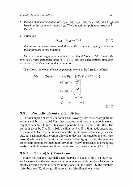
Periodic Events with Jitter 39
b) the four characteristic functions, η+EM(∆t), η−EM(∆t), δ−EM(∆t), and δ+
EM(∆t),based on the parameter tuple πEM. These functions apply to all streams inthe set.
c) a functionSEM : ΠEM �→ EM (3.15)
that returns an event stream with the specific parameters πEM provided asthe arguments to that function.
An event stream SEM is an element of an Event Model EM, if and onlyif it has a valid parameter tuple π ∈ ΠEM and the characteristic functionsassociated, that the event model defines.
This allows the model of strictly periodic events to be formally defined:
EMP = { SP(πP) | πP ∈ ΠP = {(T )|T ∈ R+ \ {0}},
η+P (∆t) =
⌈∆t
T
⌉,
η−P (∆t) =⌊
∆t
T
⌋,
δ−P (n) = (n − 1)T,
δ+P (n) = (n − 1)T}
(3.16)
3.5 Periodic Events with JitterThe assumption of strictly periodic tasks is overly restrictive. Many periodic
systems exhibit a so called jitter that captures the distortion a periodic streammight experience. Figure 3.6 shows a periodic event stream with jitter. Theperiod is given by T ∈ R
+ \ {0}, the jitter by J ∈ R+. Jitter adds uncertainty
to the model of strictly periodic events. The events arrive periodically on aver-age, but each individual event is allowed to deviate (indicated by the left-rightarrows) with respect to a virtual reference period (gray). The jitter parame-ter actually bounds the maximum deviation. Many approaches to schedulinganalysis with jitter assume a jitter that is less than the task period (J < T ).
3.5.1 The η(∆t) FunctionsFigure 3.6 contains four half-open intervals of equal width. In Figure 3.1,
we have seen that the maximum and minimum observable number of events forstrictly periodic events differs by at most one (1). In Figure 3.6, the numbersdiffer by three (3), although all intervals are left-aligned to an event.

40 Input Event Models
=3
T T T T
J J J JJ
=0
=2
=1
Figure 3.6. Time Intervals and Number of Events of Periodic Events with Jitter
T–J 2T–J 3T–J 4T–J0
+( t)
t
1
2
3
4
5
T T T T
J J J J J
–J
late
earl
y
earl
y
earl
y
earl
y
T
Jtt)(~
Figure 3.7. Upper Bound Arrival Curve of Periodic Events with Jitter
Upper-Bound Arrival Function. To which event shall the intervals bealigned? Again, the existing work on scheduling theory provides the answer.Jitter models were first considered by Locke [75]. He constructed a worstcase event arrival scenario as follows. In a stream of events, he assumed oneevent to arrive as late as possible within the maximum allowed time deviation,and all subsequently arriving events as early as possible after that first event.This scenario as well as the resulting upper bound arrival curve are drawn inFigure 3.7.
In the worst-case situation, all events in the jittered stream (except the firstone) re-arrive J earlier than in a strictly periodic stream. More precisely, onlythe first event arrives later but also the time offset of ∆t is shifted by the same

Periodic Events with Jitter 41
amount, namely the jitter J . Compared to the upper bound arrival curve of thestrictly periodic events (Fig. 3.3), the curve of the jitter stream has been shiftedto the left by J , and has the following continuous η+(∆t) function:
∀ ∆t > 0 : η+P+J(∆t) =
∆t + J
T(3.17)
The actual η+ function is given by Equation 3.18.
∀ ∆t > 0 : η+P+J(∆t) =
⌈η+(∆t)
⌉=⌈
∆t + J
T
⌉(3.18)
To demonstrate the use of such models, we briefly introduce Audsley’s jitteranalysis [4] that extends the approach of Joseph and Pandya [60] and capturesthe influence of jitter on the response time. In his model, the maximum numberof events for a given time interval is used to determine the so called worst-caseinterference Ii. Audsley calculated the response time as follows:
Ri ≤ Di = Ti (3.19)
Ri = Ji + ri (3.20)
ri = Ci + Ii (3.21)
Ii =∑
j∈HP(i)
(⌈ri + Ji
Ti
⌉︸ ︷︷ ︸
η+P+J(ri)
Cj
)(3.22)
Lower-Bound Arrival Function. A situation with the minimum num-ber is shown in Figure 3.8. The interval is right-closed half-open and alignedto an “early” event. Due to the left-openness of the interval, this event is justmissed. All other events arrive “late”, i. e. they experience the maximum de-viation. This time, the curve has been shifted to the right and the continuousη−(∆t) function is:
∀ ∆t > 0 : η−P+J(∆t) =∆t − J
T(3.23)
Since this function can be negative for ∆t less than the jitter J , the roundedvalue must be bounded to at least zero:
∀ ∆t > 0 : η−P+J(∆t) = max(
0,
⌊∆t − J
T
⌋)(3.24)
Figure 3.9 shows both the upper- and the lower-bound arrival curve. Com-pared to periodic event streams (see Figure 3.5), the uncertainty has increased.

42 Input Event Models
T+J 2T+J 3T+J 4T+J0
–( t)
t
1
2
3
4
J
J
earl
y
Jla
te
J
late
J
late
late
J
T T T T
T
Jtt)(~
Figure 3.8. Lower Bound Arrival Curve of Periodic Events with Jitter
5
0t
1
2
3
4
T
Jt
0
T
Jt
–J +J
( t)
Figure 3.9. Both Arrival Curves of Periodic Events with Jitter
3.5.2 The δ(n) FunctionsIn contrast to strictly periodic events where the distance between any two
events was constant, events with jitter can be “early” or “late”. Subsequently,the distance between events can differ.
Minimum Distance. The minimum distance δ−(2) between 2 events ina periodic stream with jitter intuitively is the period minus the jitter. The dif-ference between 3 events is one period larger, and so on. This information was
Periodic Events with Jitter 43
already used to construct the scenario with the maximum number of events,shown in Figure 3.7.
∀ n ∈ N \ {0, 1} : δ−P+J(n) = (n − 1)T − J (3.25)
Audsley exploited this property to formulate appropriate deadlines for taskswhen recurrence is prohibited. The analysis in Equations 3.19 and 3.20 illus-trate the influence of the δ− function on task deadlines:
ri ≤ Ti − Ji = δ−P+J(2) (3.26)
The windowing techniques (see Equation 3.14) can also work with periodicevents with jitter.
Maximum Distance. The maximum distance between two events is theperiod plus the jitter. The difference between three events is one period larger,and so on, leading to Equation 3.27:
∀ n ∈ N \ {0, 1} : δ+P+J(n) = (n − 1)T + J (3.27)
3.5.3 Event Model DefinitionFrom the properties of periodic event streams with jitter, we can derive the
formal definition of the model of periodic events with jitter:
EMP+J = { SP+J(πP+J) | πP+J ∈ ΠP+J ={(T, J) | T ∈ R
+ \ {0}, J ∈ R+, J < T} ,
η+P+J(∆t) =
{ ⌈∆t+J
T
⌉∆t > 0
= 0 ∆t = 0,
η−P+J(∆t) = max(
0,
⌊∆t − J
T
⌋),
δ−P+J(n) = (n − 1)T − J,
δ+P+J(n) = (n − 1)T + J}
(3.28)
The model of periodic events with jitter is very powerful. In addition tostatic, strictly periodic events, the concept of jitter allows the modeling of dy-namic event streams with uncertain, only partially known behavior within agenerally periodic stream. Basically, the regular nature of periodic events stilllays the foundation of all predictability issues, whether with jitter or not.
Besides periodic events, there is the class of aperiodic events [108] whicharrive irregularly. In general, such aperiodic events cannot be subject to anyreal-time analysis since key characteristics like the maximum number of event

44 Input Event Models
0
+( t)
t
1
2
3
4
5
d – 2d – 3d – 4d –
d – d – d – d –
d
tt)(~
Figure 3.10. Upper Bound Arrival Curve of Sporadic Events
arrivals η(∆t) can not be safely bounded. However, there is one sub-class ofaperiodic events, called sporadic events, with special properties that allow aminimum of predictability and analyzability.
3.6 Sporadic EventsIn contrast to periodic events, sporadic events arrive irregularly. There is
no average period, repetition time, or frequency. However, sporadic eventsstill allow the maximum event arrival to be bounded, since they have a knownminimum separation in time between any successive events, called the inter-arrival time d− [108, 3].
3.6.1 The η(∆t) FunctionsUpper-Bound Arrival Function. The maximum number of events canbe easily calculated from the inter-arrival time. Intuitively, the number is equalto the maximum number of events of a periodic stream with a period equal tothe inter-arrival time. In other words, the worst-case behavior (maximum num-ber of events) of a sporadic stream is a strictly periodic stream [108]. So, thesame considerations, equations, and curves can be re-used from Section 3.3.The curve is shown in Figure 3.10, and the η+ function is given by Equa-tion 3.29.

Sporadic Events 45
d –0
( t)
t
1
2
3
4
5
d
t
2d – 3d – 4d –
Figure 3.11. Both Arrival Curves of Sporadic Events
∀ ∆t > 0 : η+S (∆t) =
∆t
d−
∀ ∆t > 0 : η+S (∆t) =
⌈η+
S (∆t)⌉
=⌈
∆t
d−
⌉(3.29)
Lower-Bound Arrival Function. Sporadic events only have a mini-mum distance defined, required to bound the maximum number of events. Theminimum number is not bounded and must be assumed to be zero (0). Thatmeans, in the best case, there is not a single event occurrence:
∀ ∆t > 0 : η−S (∆t) = 0 (3.30)
The corresponding curve is trivially zero. Both curves are combined intoFigure 3.11. The figure illustrates the effect of sporadic event sources. The un-certainty linearly increases with increasing ∆t, while it is constant for periodicmodels.
3.6.2 The δ(n) FunctionsMinimum Distance. We have already mentioned that a sporadic streamshows strictly periodic properties in the worst case with maximum event ar-rival, given that TP = d−S . The η+(∆t) functions of both streams equal for all∆t. Quite similarly, also the δ−(n) function are identical. The actual functionis given by Equation 3.31. This is used by the work in [121] to find terminationconditions for the windowing technique.
∀ n ∈ N \ {0, 1} : δ−S (n) = (n − 1)d− (3.31)

46 Input Event Models
Maximum Distance. Due to the sporadic nature, the maximum distanceis infinity. In other words, sporadic events need not arrive at all:
∀ n ∈ N \ {0, 1} : δ+S (n) = ∞ (3.32)
3.6.3 Event Model DefinitionThe model of sporadic events is given by:
EMS = { SS(πS) | πS ∈ ΠS = {(d−) | d− ∈ R+ \ {0} ,
η+S (∆t) =
⌈∆t
d−
⌉,
η−S (∆t) = 0 ,
δ−S (n) = (n − 1)d−,
δ+S (n) = ∞}
(3.33)
3.7 Sporadically Periodic EventsSporadically periodic events [4] represent a specialized class of sporadic
events. Other work [121] uses the same model but refers to such streams assporadically bursty (B), where each appearance of several events is considereda burst.
A stream is characterized by three parameters. An outer period TO, definingthe minimum temporal separation of the successive bursts, a burst length bdetermining the maximum number of events within one burst, and the innerperiod T I defining a minimum distance between two events within a burst.
3.7.1 The η(∆t) FunctionsUpper-Bound Arrival Function. Again, some simple considerationshelp to construct a scenario with maximum number of events. The measure-ment interval is aligned to the first event within a burst. Subsequent events inthat burst arrive as soon as possible –similar to the “early” events in periodicstreams with jitter–, i. e. with their inner period. Each subsequent burst has thesame properties. And the bursts re-arrive as soon/often as possible, i. e. withtheir outer period. A scenario with a burst length of b = 4 and the correspond-ing upper-bound arrival curve is shown in Figure 3.12. The curve illustratesbursts and idle periods. It shows the (worst-case) periodic nature “within” aburst as well as the sporadic nature of the appearance of the “bursts” itself.The η+(∆t) function is given by Equation 3.34. The equation separates: a)a number of � ∆t
T O � full bursts of b events each, and b) the remaining sporadicevents in the remaining time interval ∆t − � ∆t
T O �TO, eventually bounded by

Sporadically Periodic Events 47
0t
3
4
5
7
1
2
3TI2TITI
6
+( t)
8
TO+TI TO+3 TI
TO TO+2 TI
b b
IinnerT
tt)(~
OouterT
tbt)(~
Figure 3.12. Upper Bound Arrival Curve of Sporadically Periodic Events
the maximum burst length b.
∀ ∆t > 0 : η+B (∆t) =
⌊∆t
TO
⌋b︸ ︷︷ ︸
full bursts
+ min
(⌈∆t − ⌊ ∆t
T O
⌋TO
T I
⌉, b
)︸ ︷︷ ︸
remaining events
(3.34)
This function can be found in the response time approaches of Tindell [121]and Audsley [4].
In contrast to the three other models, no equally simple continuous η+ func-tion exists. We can, however, provide two continuous ones, each one focusingon a different issue of sporadically periodic events. When we apply the innerperiod to η+
P of equation 3.9, we obtain η+inner bounding the maximum fre-
quency during bursts in Figure 3.12. Similarly, we can find η+outer when using
the outer period and the burst length, providing a long-term average number ofevents. Both these curves are shown in Figure 3.12.
Lower-Bound Arrival Function. Sporadically periodic events –as ageneralized class of sporadic events– do not need to appear at all. Hence, theη− function is assumed zero:
∀ ∆t > 0 : η−B (∆t) = 0 (3.35)

48 Input Event Models
0t
3
4
5
7
1
2
6
( t)
8
IT
t
OT
tb
3TI2TITI TO
Figure 3.13. Both Arrival Curves of Sporadically Periodic Events
Both event arrival curves are combined in Figure 3.13.
3.7.2 The δ(n) FunctionsMinimum Distance. Similar to Equation 3.34, the actual calculation ofthe minimum distance δ−(n) distinguishes full bursts and a remainder:
∀ n ∈ N \ {0, 1} : δ−B (n) =⌊
n − 1b
⌋TO
︸ ︷︷ ︸full bursts
+ ((n − 1) −⌊
n − 1b
⌋b)T I
︸ ︷︷ ︸remaining events
(3.36)
Maximum Distance. The maximum event distance of any sporadic eventstream is infinity:
∀ n ∈ N \ {0, 1} : δ+B (n) = ∞ (3.37)

Summary 49
3.7.3 Event Model DefinitionThe model of sporadically periodic events is given by:
EMB = { SB(πB) |πB ∈ ΠB = {(TO, T I , b) | TO ∈ R
+ \ {0}, T I ∈ R+,
b ∈ N+ \ {0}, TO ≥ T I × b} ,
η+B (∆t) =
⌊∆t
TO
⌋b + min
(⌈∆t − ⌊ ∆t
T O
⌋TO
T I
⌉, b
),
η−B (∆t) = 0 ,
δ−B (n) =⌊
n − 1b
⌋TO + ((n − 1) −
⌊n − 1
b
⌋b) T I ,
δ+B (n) = ∞}
(3.38)
3.8 SummaryThe use of abstract event stream is essential for many scheduling analysis
techniques such as RMS (rate-monotonic scheduling). We have defined eventstreams and event models, and we have reviewed the four most popular eventmodels in literature: strictly periodic (P), periodic with jitter (P+J), sporadic(S), and sporadically periodic or sporadic bursts (B). These models requireonly a few key parameters in order to describe the behavior of a stream.
Using examples such as in Equations 3.7 and 3.22, we have shown howthese parameters are used in scheduling analysis. Four characteristic func-tions apply to all event streams. For instance, the maximum number of eventsη+(∆t) is required to determine the number of preemptions of a task. Theminimum distance between events δ−(n) is used to restrict task deadlines (seeEquation3.26) or to correctly capture for task recurrence as in Equation 3.14.These two functions capture the key event stream properties in the area ofclassical scheduling analysis that targets maximum (worst-case) task and com-munication response times. Approaches that target distributed systems addi-tionally require the minimum number of events and the maximum distance, todetermine minimum response times, in turn required to resolve system-levelscheduling anomalies. We have explained these effects in Section 2.2.2. Weconclude this chapter with an overview of the characteristic functions of thefour event models in Table 3.1.

50 Input Event Models
πη
+(∆
t)η−(∆
t)δ−
(n)
δ+(n
)
PT
⌈ ∆t
T
⌉⌊ ∆
t
T
⌋(n
−1)
T(n
−1)
T
P+
JT
,J
⌈ ∆t+
J
T
⌉m
ax( 0,
⌊ ∆t−
J
T
⌋)(n
−1)
T−
J(n
−1)
T+
J
Sd−
⌈ ∆t
d−
⌉0
(n−
1)d−
∞
BT
O,T
I,d
⌊ ∆t
TO
⌋ b+0
⌊ n−
1b
⌋ TO+
∞
min
(⌈ ∆t−⌊ ∆t T
O
⌋ TO
TI
⌉ ,b
)( (n
−1)−
⌊ n−
1b
⌋ b)T
I
Table 3.1. Parameters and Characteristic Functions of the Four Most Popular Event Models
Chapter 4
OUTPUT EVENT MODELS
We have seen how event models are used to capture task activation. Strictlyperiodic events, for instance, might be generated by a timer interrupt. The othermodels, however, aim at capturing the partially non-deterministic behavior ofevent sources, i. e. other tasks that produce the events that activate tasks. Thisalready shows that event timing needs not only be considered at task input butalso at task’s outputs.
This chapter investigates task input-output timing behavior and specificallyanalyzes the output event generation. This is absolutely necessary for the com-ponent integration step mentioned in Section 2.5. One task’s output becomesanother task’s input. We also need appropriate output event models, otherwisetwo models cannot be reasonably coupled [101, 98]. The key goal in this con-text is a consistent and systematic use of event models.
We use expressive examples to introduce the basic concepts of output mod-eling. We start with simple, constrained task configurations such as periodictasks with deterministic timing behavior. We then gradually add more con-cepts, especially all possible sources of non-determinism like jitters, sporadicevent sources, and conditional task execution.
4.1 Periodic Task ActivationWe have mentioned in Section 3.1 that task activation can always be mod-
eled as event triggered, if we can properly describe the event sources that pro-duce these events. However so far, only relatively simple event sources havebeen considered, such as a system timer with a fixed frequency. Such eventgeneration is a form of output production, the timer outputs events, and canbe described using the periodic event model. In the local analysis techniquesmentioned in Section 2.1, such event models are directly used as input eventmodels, i. e. activating events, for a task.

52 Output Event Models
input
output
R constant response time
T1
(a) Constant Response Time
T T T T
T
input:
periodic
output:
periodic
RT
RRT
RT
R
input-output delay
(b) Periodic Input and Periodic Output
Figure 4.1. Periodic Task with Constant Response Time
4.1.1 Constant Response TimesPeriodic output production generally applies to all tasks that are activated
periodically and have a constant input-output delay, i. e. a constant responsetime. In this thesis we assume that a task produces its output on completion.So the output generation times of the ith output are equal to the task completiontimes of the ith task execution:
tout(i) = tin(i) + R(i) (4.1)
A periodic task T1 with a constant response time together with its periodicinput and output streams is shown in Figure 4.1(a). It is quite clear that, exceptin the case of a constant phase delay which is not considered by event models,both input and output streams have equivalent properties, they are identical:
S1,out = S1,in = SP(Tin) (4.2)
4.1.2 Response Time Intervals and Output JitterSuch a simple and static input-output behavior is, however, not commonly
the case. Sophisticated architectures include pipelines and caches might stallthe task, i. e. enforce wait cycles, in a seemingly non-deterministic manner.Secondly, the task might have a data-dependent control flow using if-then-else statements or data-dependent loop counts. Scheduling introduces de-lays that far exceed other architecture influences. Depending on the behav-ior of other tasks on the same resource, the number of preemptions can be

Periodic Task Activation 53
input
output
R–
R+
response time interval with
response time jitter
JR
T1
(a) Non-Constant Response Time
R– R R+ R+
T T T T
R– R+ R– R R+
earl
y
late
late
T
input:
periodic
output:
periodic with jitter JRJR
(b) Periodic Output with Jitter
Figure 4.2. Inheritance of Response Time Jitter at Task Output
smaller or larger. We have already seen such tasks in the introduction (seeFigure 1.3). The result is a non-constant task response time, represented by aninterval constrained by upper and lower response time bounds, as indicated inFigure 4.2(a):
R1(i) ∈ R1 = [R−1 ; R+
1 ] (4.3)
Even if activated strictly periodically, the output of such a task inherits theresponse time jitter J1,R. Figure 4.2(b) shows an execution scenario with vary-ing response times. The minimum or shortest response time results in an earlyoutput while the maximum response leads to a late output. So, the output jitterequals the response time jitter which is the difference between the two responsetime interval bounds:
J1,out = J1,R = R+1 − R−
1 (4.4)
The output stream of task T1 is:
S1,out = SP+J(T1,in, R+1 − R−
1 ) (4.5)
4.1.3 Inheritance of Input JitterSuch periodic streams with jitter can activate other tasks. Figure 4.1.3 shows
a chain of tasks. Task T1 is taken from the previous example and is known tohave a strictly periodic activation and an output jitter. This output jitter turnsinto the input jitter of task T2.

54 Output Event Models
T1
periodic periodic w/ jitter
T2 T3T4
? ? ?
R3–
R3+
R2–
R2+
R1–
R1+
R4–
R4+
Figure 4.3. Non-Constant Response Times in a Task Chain
R3–
R2–
R1–
R4–
R3+
R2+
R1+
R4+
J2,in = J1,out
early
late
J3,in = J2,out
J4,in = J3,out
J4,out
Figure 4.4. Early and Late Scheduling Diagrams
Tindell and Clark [122] studied such systems and they recognized that apossible input jitter is also inherited at the task’s output, just as the (internal)response time jitter is inherited. In other words, the response time jitters accu-mulate along a task chain, where each task adds its response time jitter frominput to output:
Ji,out = Ji,in + Ji,R
= Ji,in + (R+i − R−
i ) (4.6)
Hence, the output stream is given by:
Si,out = SP+J(Ti,in, Ji,in + Ji,R) (4.7)
The early and late execution sequence diagrams and the jitter accumulationare shown in Figure 4.3.
The jitter plays an important role in system-level scheduling. It capturesthe scheduling influences of one task at the input of another. This is also thebasic underlying idea of the holistic analysis techniques published by Tindelland Clark [122] and Gutierrez, Palencia, and Harbour[41]. They establish re-sponse time equations for each task in the system. For dependent tasks, theseequations are mutually dependent, resulting in a complex equation set to besolved.

Periodic Task Activation 55
Best-case response times R− were initially simply considered zero, result-ing in unnecessarily large jitters. Since then, many improvements of best-caseanalysis have been proposed. Tindell [120] captured static phase information,the phase delay between the activation of two successive tasks. He called thisphase offset [120] within a transaction. Palencia and Harbour [82] extendedthis approach to dynamic offsets. Other groups have been studying best-caseanalysis, too [62, 47, 92, 49]. Interestingly, most of the work is done no ear-lier than 30 years after Graham forecasted an increase in the importance ofbest-case analysis when resolving scheduling anomalies [37].
4.1.4 Event Streams with Large JittersImproving best-case analysis helps to increase the accuracy of the jitter cal-
culation. The improvements, however, do not reduce the actual jitter, whichmonotonically increases along task chains and can even exceed the originalperiod. We mentioned in Section 3.5 that many of the known scheduling andanalysis techniques require jitters less than periods to be applicable. A jitterequal to the period would result in the simultaneous arrival of two task activa-tions, in turn leading to task recurrence. Not all analysis approaches considerrecurrence but require that one execution is finished before the next activationarrives.
There are few extensions. Lehoczky [69] and Tindell [121] introduced thenotion of arbitrary deadlines and presented response time analysis techniquesthat are not restricted to any deadlines. Their techniques allow for large jitters,and we extend the jitter model from Section 3.5 by allowing arbitrary jitters:
πP+J ∈ ΠP+J = {(T, J)|T ∈ R+ \ {0}, J ∈ R
+} (4.8)
The consequences on the characteristic functions are explained in the followingsections.
4.1.4.1 The η(∆t) FunctionsUpper-Bound Arrival Function. To construct the upper bound arrivalscenario, we apply the well known technique from Section 3.5. We assumethe first event arriving as late as possible and all others arriving as early aspossible. This has already been used in constructing worst-case event arrivalin the previous chapter. Figure 4.5 shows an upper bound arrival for an eventstream where the jitter is larger than the period. The curve has almost thesame properties as the curves of streams with jitters less than periods. So, theη+(∆t) function can be reused from Equation 3.18 in Section 3.5:
∀ ∆t > 0 : η+P+J(∆t) =
⌈∆t + J
T
⌉(4.9)

56 Output Event Models
0
+( t)
t
3
4
5
6
1
2
3T–J 4T–J 5T–J
T T T T
J
Tearl
y
late earl
y
earl
y
–J
wait
T
Jtt)(~
Figure 4.5. Upper-Bound Arrival Curve of Periodic Events with “Large” Jitter
There are, however, some important differences between jitter less than pe-riods, and jitter equal to or larger than periods. In Figure 4.5, we see thatthe first three events now arrive seemingly simultaneously, i. e. within an in-terval of ∆t = 0 time units. But for reasons explained in Section 3.3.1, theη(∆t) function is defined to be zero at ∆t = 0. To calculate the numberof events that arrive simultaneously (n0), we need to determine the limes for∆t → 0, ∆t > 0:
n0 = lim∆t→0,∆t>0
η+(∆t) =⌊
J
T
⌋+ 1
Another important observation in Figure 4.5 is that the second and thirdevent also experience a delay, although they should be assumed early. Thisis because events in a stream must usually maintain the order in which theyarrive, i. e. events are not allowed to “overtake” each other and thus have to“wait”. This preserves the causality of input and output streams of a task,and it is also the best strategy to reduce the maximum “waiting time” of eachindividual event. Hence, the second and third event cannot be early in the senseof immediately. This is an important property of large jitters. In other words,there is an implicit minimum inter-arrival time of zero that preserves the orderof events.

Implications of Large Jitters 57
0
+( t)
t
3
1
2
earl
y
late
late
J
T T T T
J
T+J 2T+J+J
T
Jtt)(~
Figure 4.6. Lower- Bound Arrival Curve of Periodic Events with “Large” Jitter
Lower-Bound Arrival Function. The lower bound arrival curve isshown in Figure 4.6. Clearly, the function known from small jitters (Sec. 3.5)applies which was already given by Equation 3.24:
∀ ∆t > 0 : η−P+J(∆t) = max(
0,
⌈∆t − J
T
⌉)(4.10)
4.1.4.2 The δ(n) FunctionsThe fact that several events can arrive simultaneously also affects the δ−(n)
function. Other than in Equation 3.25, the minimum distance between twoevents can be zero. In the above example it is even zero for n = 3. The actualδ−(n) function is given by Equation 4.11:
∀ n ∈ N,n ≥ 2 : δ−P+J(n) = max (0, (n − 1)T − J) (4.11)
The maximum distance between events is not affected in concept. The equa-tions from the jitter model as introduced in Section 3.5 are still valid:
∀ n ∈ N,n ≥ 2 : δ+P+J(n) = (n − 1)T + J (4.12)
4.2 Implications of Large JittersA key property of streams with large jitters (we will use the formulation
large jitter for jitter larger than the period) is the possibly simultaneous arrivalof events. However, tasks are not usually activated simultaneously but witha certain delay. The execution sequence of Figure 4.7 provides an example.

58 Output Event Models
T3
T1
T2
prio
rity
T1
T2
T3
T3 response times
maximum
minimum
T3
T2
T1
buffering
Figure 4.7. An Example of Output Events with “Large” Jitter
Point-To-Point Link
T2
T1
T3
CPU1
RTOS1
T5
T4
CPU2
RTOS2
periodic with large jitter
Figure 4.8. Distributed System Example
It contains a zoomed view of Figure 1.4 and shows the worst-case bufferingscenario of task T3.
All tasks are activated periodically without any input jitter. Scheduling fol-lows static priorities, T1 has the highest and T3 the lowest priority. The periodsare T1, T2, and T3, respectively. Task T3 is blocked for several periods andthen executes several times in a row (bursty). The scheduling diagram illus-trates that the response time jitter (the best-case to worst-case difference) farexceeds the period. In other words, task T3 has a large output jitter. We willnow analyze the effect of this large output jitter on the scheduling and analysisof other tasks.
4.2.1 Propagation of Large JittersFigure 4.8 shows a distributed system. CPU1 scheduling has just been an-
alyzed above. We use the output stream of T3 to determine the activation and

Implications of Large Jitters 59
n0,4 T4 – J4
T5
prio
rity
T5 response times
T4 response times
maximum
minimum
T4
n0 simultaneous events
T4
T5
T5
maximum minimum
Figure 4.9. Scheduling with Simultaneous Task Activation due to Large Jitters
execution behavior of T4 in CPU2 scheduling analysis. First, we must propa-gate the stream parameters:
S4,in = S3,out
= SP+J(T3, J3,R)
Now, we can perform all kinds of scheduling analyses based on this T4 in-put stream representation. We assume that scheduling follows static prioritieswhere task T4 has a higher priority than task T5. Figure 4.9 shows a schedulingdiagram of the second resource.
Due to the large jitter, worst-case scheduling analysis for both tasks mustassume the simultaneous arrival of n0,4 task T4 activations, just as introducedin Section 4.1.4.1. In effect, task T4 is simultaneously activated and the cor-responding executions interfere with each other. This has two important con-sequences. Firstly, task T4 has a large maximum response time and –again– alarge output jitter. Secondly, this burst execution also leads to a large maximumresponse time for task T5. After the burst phase is over, the first task activationunder “normal” conditions arrives at n0,4 T4 − J4 after the beginning of theburst.
It is quite obvious that the simultaneous arrival of multiple task activationshas a major (negative) impact on the maximum response times and subse-quently to the response time jitters and the overall jitters in the system; andlarge jitters, in turn, lead to the assumption of simultaneous events. The exam-ples show that scheduling dependencies and input jitter inheritance and accu-

60 Output Event Models
T4
T5
prio
rity T4 response times
T4
T5
T5 response times
T5
minimummaximum
T3
T4n0,4 T4 – J4
Figure 4.10. Scheduling with Large Jitter but Bounded Inter-Arrival Time
mulation (see Sec. 4.1.3) can quickly lead to extremely large jitters and sub-sequently to high transient loads and wide response time intervals. Reducingthe pessimism in the jitter analysis is a critical task, since it results in lesspessimistic response times. Tighter response time intervals, in turn, result intighter jitters.
4.2.2 Limitations and InefficienciesIn practice, simultaneous activations of the same task rarely occur as a result
of jitter. When we take a closer look at the execution and scheduling of thetasks, particularly task T3 on the resource CPU1 (Fig. 4.7) , we see that theoutput events are not produced simultaneously, although it executes severaltimes in a row. Hence, T4 on resource CPU2 is not activated simultaneously.Figure 4.10 shows a scheduling scenario where activations arrive one afteranother instead of simultaneously. For comprehensibility, the scheduling oftask T3 on the CPU1 is included in the figure. Task T4 is activated when taskT3 finishes.
Compared to the situation of simultaneous activation, we observe vast im-provements in worst-case response times for both tasks, T4 and T5. Task T4
does not interfere with itself and the variations in the response time are little,if we assume a relatively constant core execution time. Furthermore, the sameeffect (no burst execution of T4) allows task T5 to exploit the “gaps” in theschedule, so T5 experiences at most two preemptions by T4, compared to fivein the case of simultaneous T4 activation (see Fig. 4.9). For a better under-

Implications of Large Jitters 61
T4
T5
prio
rity
bounded maximum frequency
simultaneous arrival
simultaneous
arrival
reduction of maximum
T4 response time
reduction of maximum
T5 response time
T5
T4
T4
T4
T5
T4
T5
T4
Figure 4.11. Comparison between two Schedules
standing, Figure 4.11 shows a detailed comparison between the two schedules.The reductions in the maximum response time bound are highlighted. Thesedirectly translate into reductions of the output jitter pessimism.
This optimization was possible since task T3 does not output events simul-taneously, but with a certain amount of time between two successive events.The knowledge that there is a time separation between the events originatesfrom detailed information about the execution and scheduling of T3 on CPU1.Unfortunately, this information is not preserved in the output stream represen-tation, simply because the model of periodic events with jitter is unable to cap-ture this property. In other words, the information is lost in the output streamrepresentation. Subsequently, CPU2 analysis must assume simultaneous eventarrival, with the known inefficiencies.
4.2.3 Modeling AlternativesThe model of periodic events with large jitter has critical limitations in its
expressive power. In order to exploit the non-simultaneous arrival of eventsin scheduling analysis of CPU2, we need an event stream representation thatutilizes such information.

62 Output Event Models
We have summarized in Section 3.7 the model of sporadically periodicevents or sporadic bursts. This event model has a notion of a minimum inter-arrival time or inner period that provides the required concepts to prevent si-multaneous event arrival. The model thereby bounds the maximum transientevent frequencies during bursts, just as observed in the above example. So, thisevent model is able to capture the non-simultaneous property of output events.
But the model of sporadically periodic events has another limitation: it isbased on sporadic events and is thus unable to capture the periodic nature ofthe original input stream. In effect, best case analysis potentially assumes toofew preemptions, resulting in underestimations for the minimum response timeof tasks, in turn leading to larger output jitters. So, what else can we do?
In Figure 4.7, we have observed a known temporal separation betweenevents in periodic streams with jitter. Therefore, we also introduce the conceptof minimum inter-arrival to periodic models with jitter as a direct extension forlarge jitter support.
Quite interestingly, this extension has never been proposed before. Thismeans that, as yet, no event model exists to capture the effects of increasingjitter in distributed, periodic systems to a reasonable level of accuracy. Con-versely, the existing models seem more a collection of independently definedformalisms rather than a sound and systematic way to capture the key effectsof scheduling and execution in distributed environments. These insufficiencieslead to overly conservative results which considerably degrades system-levelanalysis possibilities.
4.3 A New Model: Periodic Events with BurstWe introduce the idea of a minimum inter-arrival time or inner period to the
model of periodic events with jitter. The result is a very powerful model whichwe call periodic events with burst (P+B) as a direct extension of the standardjitter model. A periodic stream with burst is characterized by three parameters.A period T , a jitter J , and a minimum event distance d. Simply speaking, themodel captures a normal jitter, just as introduced in Section 3.5. Additionallythe maximum transient event frequency is bounded, just as in the model ofsporadically periodic events (see Section 3.7).
The event model of periodic events with burst is given by:
EMP+B = { SP+B(πP+B) |πP+B ∈ ΠP+B = {(T, J, d) | T ∈ R
+ \ {0}, J ∈ R+, d ∈ R
+} ,
η+P+B(∆t), η−P+B(∆t), δ−P+B(n), δ+
P+B(n)}(4.13)
The four characteristic functions are introduced in the following sections.

A New Model: Periodic Events with Burst 63
0
+( t)
t
3
4
5
6
5
1
2
T
Jt
d
t
4T–J 5T–J 6T–J3d –2d –d 7T–J
sporadic stream
characteristics
during burst
jitter characteristics during non-bursts
T
Jttjitter )(~
d
ttsporadic )(~
Figure 4.12. Upper-Bound Arrival Curve of Periodic Events with Burst: “Large” Jitter and aMinimum Distance
4.3.1 The η(∆t) FunctionsUpper-Bound Arrival Function. Figure 4.12 shows the resulting up-per bound arrival curve. We can distinguish two regions for ∆t, each regiondominated by another effect. Large values of ∆t reflect the long term behav-ior of the stream that is periodic with jitter. Under this “normal” behavior, thestream is characterized by its large jitter, just as mentioned in Section 4.1.4.The curve can be described by Equation 4.9.
Small ∆ts capture the behavior during bursts, and the worst-case arrival isdominated by the minimum event distance d to bound the maximum transientfrequency during the burst. Such behavior is already known from the two spo-radic models in Sections 3.6 and 3.7, and the curve is given by Equation 3.29.After the burst has finished, the event stream returns to its “normal” behavior.
Basically, both effects (and the corresponding η+ functions) overlap eachother. Both bound the maximum number of events. The resulting η+(∆t)function is the minimum of the two individual functions:
∀ ∆t > 0 : η+P+B(∆t) = min
(⌈∆t
d
⌉,
⌈∆t + J
T
⌉)(4.14)

64 Output Event Models
0
( t)
3
4
5
6
5
T
Jt
1
2d
t
t
T
Jt
+JFigure 4.13. Upper- and Lower-Bound Arrival Curves of Periodic Events with Burst
The transition from the “burst” phase into the “normal” operation appearsat the intersection of the curves of the two regions; more precisely, at the inter-section of the corresponding continuous curves:
η+sporadic region(∆t) = η+
jitter region(∆t)⇔ ∆t
d = ∆t+JT
⇔ ∆t = J dT−d
(4.15)
Lower-Bound Arrival Function. The minimum distance has been in-troduced to bound the maximum event frequencies. The lower bound functionusually deals with minimum frequencies and is not influenced by the newlyadded property, and it equals the one given by Equation 4.10 in Section 4.1.4:
∀ ∆t > 0 : η−P+B(∆t) = max(
0,
⌈∆t − J
T
⌉)(4.16)
The corresponding η−(∆t) curve has already been introduced in Figure 4.6.Both upper and lower bound arrival curves are shown in Figure 4.13.
4.3.2 The δ(n) FunctionsMinimum Distance. Since we have introduced a parameter boundingthe minimum distance between two successive events, the δ(n) functions alsochange compared to the function from large jitters as introduced in Section 4.1.4.Similar to the η+ function, two regions can be distinguished, each dominated

Sporadic Task Activation 65
by another effect. During the burst phase, the sporadic nature of minimumevent distance dominates, while the period and jitter dominate the other re-gion. The function is given by the following equation:
∀ n ∈ N,n ≥ 2 : δ−P+B(n) = max ((n − 1)d , (n − 1)T − J) (4.17)
Maximum Distance. Similar to the lower-bound event arrival function,the maximum distance is not affected by the proposed extension, and the func-tion from the “normal” jitter model as given by Equation 3.27 applies:
∀ n ∈ N,n ≥ 2 : δ+P+B(n) = δ+
P+J(n) = (n − 1)T + J (4.18)
4.3.3 Bounding the Minimum Output DistanceDuring bursts, several executions or instances of a single task interfere with
each other, as seen in Figures 4.7 and 4.9, they are re-activated before previousactivations have completed. This effect is known as task recurrence [69, 121].In practice, such situations could eventually be handled in several ways in-cluding the termination (kill) of the current task instance or a real preemption.Such implementations, however, do not guarantee causality between input andoutput event streams, and they are not considered further here.
We want to guarantee input-output causality, hence a newly arriving taskactivation must be blocked until all preceding activations have successfullycompleted. Examples are given in Figures 4.7 and 4.9. A task requires at leastits minimum response time to execute. Hence, the minimum response timerepresents an additional lower bound on the minimum output distance duringoutput bursts. Finally, there is a third bound that might dominate the outputduring input bursts:
Si,out = SP+B
(Ti,out = Ti,in ,
Ji,out = Ji,in + Ji,R ,
di,out = max(Ti,out − Ji,out︸ ︷︷ ︸
as with jitter
, R−i︸︷︷︸
duringoutputbursts
, di,in − Ji,R︸ ︷︷ ︸during input bursts
) )
(4.19)
The third bound is related to transient frequencies that increase from input tooutput, similar to the increase in jitter, and is explained in detail in the nextsection.
4.4 Sporadic Task ActivationWhile periodic events (with or without jitter) have a certainly deterministic
behavior, i. e. their arrival can be predicted to a certain extent, sporadic events

66 Output Event Models
input:
sporadic
output:
sporadic
input-output delay
input
output
R constant response time
T1
R R R R
d–int1>d–
in t2>d–in
d–out=d–
in
t1>d–out t2>d–
out
1 2 3 4
Figure 4.14. Sporadic Task Execution with Constant Response Time
arrive seemingly irregularly. Sporadic task activation models have proven pow-erful in modeling the behavior of such non-deterministic event sources, forinstance customer requests to servers. Details have already been reviewed inSection 3.6. This section focuses on the effect of execution and schedulingon the properties of sporadic event streams, just as we have done above forperiodic streams.
4.4.1 Constant Response TimeA constant response time represents a constant input-output delay, and the
task output equals the task input except a constant phase delay. We have al-ready observed this behavior for periodic events in Section 4.1.1. Hence, theoutput stream equals the input stream:
S1,out = S1,in = SS(d−1,in) (4.20)
4.4.2 Response Time IntervalSporadic events that enter a system experience the same types of distortion
as periodic events. The stream timing changes from a task’s input to the task’soutput, response time intervals lead to increasing uncertainty about the outputevent arrival curves. We have already analyzed the effects of non-constantresponse times to task input-output timing in Section 4.1.2. In the case ofperiodic events, we could easily use the known jitter event model to capturethis effect. But the concept of a jitter is unknown for sporadic events whichonly define a minimum inter-arrival time. So, we need a different approach.
The worst-case situation is shown in Figure 4.15. Two effects contribute tothe “worst-caseness” here: a) the two task activations arrive with their mini-mum inter-arrival time, i. e. no other two successive task activations will everarrive closer in time, and b) a “late” output event is followed by an “early”

Sporadic Task Activation 67
d–in
R–R+
earl
y
late
input
output
tout = d–out = d–
in – JR
tout
Figure 4.15. Worst-Case Output Timing of Sporadic Tasks
one, i. e. the response time jitter reduces the event distance from input to out-put further, just as already known from jitters (see Sec. 4.1.3). Essentially bothmentioned effects must coincide to yield the worst case. A larger input distancewill result in a larger output distance, as will a different response time distri-bution. From these observations, we can calculate the sought-after minimumoutput inter-arrival time:
Si,out = SS(d−i,out = d−i,in − Ji,R) (4.21)
This also represents the third bound in Equation 4.19.
4.4.3 Decreasing Inter-Arrival TimesSimilar to increasing jitters, the minimum inter-arrival time usually decreases
from input to output, the amount of decrease is the response time jitter. If weconsider a chain of several tasks, we can easily imagine that the reduction givenby Equation 4.21 could theoretically lead to negative results for dout. Clearly,negative event distances simply do not make any sense, and a zero minimuminter-arrival time translates into a infinite worst-case event frequency, we wouldneed to assume an infinite number of events all arriving simultaneously.
We have already discussed the problem of simultaneous event arrival in Sec-tion 4.2.2 for the jitter model. We introduced the notion of an output event dis-tance as an additional bound to the basic jitter model (which we now call themodel of periodic events with burst). And we could show that the minimumresponse time bounds this output distance. This bound not only applies to theoutput event distance in the newly introduced model of periodic events withburst (see Equation 4.19). It is a general bound on the output timing of anytask and also applies to the model of sporadic events, and Equation 4.21 turnsinto:
Si,out = SS
(d−i,out = max
(d−i,in − Ji,R, R−
i
))(4.22)
4.4.4 Sporadically Periodic Task ActivationThe model of sporadically periodic events (or sporadic bursts) from Sec-
tion 3.7 also defines a minimum inter-arrival time, also called inner period T I
(see Section 3.7). The minimum response time represents a bound to this inner

68 Output Event Models
period, too. Furthermore, the response time jitter, introduced in Section 4.1.2,influences both the inner and the outer output period:
Si,out = SB
(TO
i,out = max(TO
i,in − Ji,R, bi,in × T Ii,out︸ ︷︷ ︸
mathematical bound
),
T Ii,out = max
(T I
i,in − Ji,R, R−i
),
bi,out = bi,in
)(4.23)
The mathematical bound on the outer period captures the fact that the maxi-mum average frequency b
T O does not exceed the maximum transient frequencybounded by 1
T I .
4.5 Conditional Output GenerationThe previous section focused on the propagation of sporadic event streams
that are inputed into a system from its environment. However, sporadic envi-ronments are not the only source for sporadic events, they can also result fromoriginally periodic sources in the presence of conditional communication.
Conditional output generation means that a task does or does not produceoutput events, and the decision depends on the results of some calculationsinternal to the task, for instance within either the then or the else block ofan if-then-else statement. In other words, the output production dependson the internal functionality of the task. Scheduling analysis often abstractsfrom such internal functional details and only looks at relatively simple cornercases of task execution without considering the conditions that lead to eithercase.
4.5.1 Constant Response TimesAgain, we start with the situation of a constant response time. We can iden-
tify two corner-case scenarios. In the scenario of Figure 4.16(a), the task al-ways produces an event at completion time. This obviously results in a purelyperiodic output, just as introduced in the case of unconditional output produc-tion (see the introduction of this chapter). The other extreme is a scenario inwhich the task never produces any output. This is illustrated in Figure 4.16(b).
One already introduced model that captures such behavior is the model ofsporadic events. Figure 3.11 in Section 3.6 nicely illustrates the two behavioralcorner-cases. So, conditional output production transforms a periodic inputstream into a sporadic output stream:
Si,out = SS(Ti,in) (4.24)

Conditional Output Generation 69
input:
periodic
output:
periodic
T T T
R
t=T
T T T
R
t=T
R
t=T
R
t=T
R
t=T
R
t=T
R
(a) “Always” Output
input:
periodic
output:
"none"
T T T
R
T T T
R R RRRRno
outputno
outputno
outputno
outputno
outputno
outputno
output
t
(b) “Never” Output
Figure 4.16. Two Corner Cases of Conditional Output Production
4.5.2 Response Time IntervalsThe situation is more complex when we consider response time intervals.
Again, we can distinguish two corner-case scenarios. In the “always output”scenario, the output is periodic with jitter as introduced in Section 4.1.3. Andfor the “no output” scenario, we need some kind of sporadic model. However,a model capturing periodic with jitter as one bound and “no output” as the otherbound is not known in literature. The same applies to conditional tasks that areactivated periodically with burst. We have to resort to the model of strictlysporadic events. The minimum inter-arrival time is calculated according to theobservations from increasing jitters in generally periodic streams. This is validbecause the periodic stream with jitter represents the upper output bound, andthe sporadic model defines an upper bound, only:
Si,out = SS
(max
(Ti,in − Ji,R, R−
i
))(4.25)
4.5.3 Input with Jitter and BurstIf the task is already activated with a jitter (or even burst), then we can easily
extend Equation 4.25:
Si,out = SS
(max
(Ti,in − Ji,in − Ji,R, di,in − Ji,R, R−
i
))(4.26)
We see that the minimum inter-arrival time continually decreases alongtask chains, representing increasing frequencies. These increasing frequen-

70 Output Event Models
0
( t)
t
3
4
5
6
5
1
2
3T–J 4T–J 5T–J 6T–J
T
Jt
Figure 4.17. Upper- and Lower-Bound Arrival Curves of Sporadic Events with Jitter
cies, however, are not a property of the actual system behavior but of the eventstream representation that suffers from considerable modeling inefficiencies.
4.6 New Sporadic Models with Jitter and BurstSo far, we have identified two key effects that task execution and schedul-
ing impose on output event streams: a) jitters increase from inputs to outputs(see Sec. 4.1.3) and finally lead to bursts (Sec. 4.3), and b) conditional com-munication turns periodic inputs into sporadic output behavior (Sec. 4.5). Thetwo effects are apparently orthogonal, and it is relatively straight-forward tocombine the already known concepts used to capture both individual effects.
4.6.1 Sporadic Events with JitterWe extend the sporadic model to also capture a possible input jitter. The
model of sporadic events with jitter is defined by:
EMS+J = { SS+J(πS+J) |πS+J ∈ ΠS+J = {(T, J)|T ∈ R
+ \ {0}, J ∈ R+} ,
η+S+J(∆t), η−S+J(∆t), δ−S+J(n), δ+
S+J(n)}(4.27)
with the characteristic functions defined below.

New Sporadic Models with Jitter and Burst 71
0
( t)
3
4
5
6
5
T
Jt
1
2d
t
t
Figure 4.18. Upper- and Lower-Bound Arrival Curves of Sporadic Events with Burst
In the “always” case, periodic with jitter provides an upper bound on η+(∆t)and a lower bound on δ−(n):
∀ ∆t > 0 : η+S+J(∆t) = η+
P+J(∆t) =⌈
∆t + J
T
⌉(4.28)
∀ n ∈ N,n ≥ 2 : δ−S+J(n) = δ−P+J(n) = max (0, (n − 1)T − J) (4.29)
In the other case, the bounds are zero for η−(∆t), and infinity for δ+(n) re-spectively, formally capturing the sporadic nature of the model. We call thismodel sporadic events with jitter, with the index S+J. The combined upperand lower bound arrival curves are shown in Figure 4.17.
4.6.2 Sporadic Events with BurstTo avoid the inefficiencies of large jitters, we also define the model of spo-
radic events with burst (S+B):
EMS+B = { SS+B(πS+B) |πS+B ∈ ΠS+B = {(T, J, d) | T ∈ R
+ \ {0}, J ∈ R+, d ∈ R
+} ,
η+S+B(∆t), η−S+B(∆t), δ−S+B(n), δ+
S+B(n)}(4.30)
The combined upper and lower bound arrival curves are shown in Fig-ure 4.18. The characteristic functions are given by:
∀ ∆t > 0 : η+S+B(∆t) = η+
P+B(∆t) = min(⌈
∆t
d
⌉,
⌈∆t + J
T
⌉)(4.31)

72 Output Event Models
∀ ∆t > 0 : η−S+B(∆t) = 0 (4.32)
∀ n ∈ N,n ≥ 2 : δ−S+B(n) = δ−P+B(n) = max ((n − 1)d , (n − 1)T − J)(4.33)
∀ n ∈ N,n ≥ 2 : δ+S+B(n) = ∞ (4.34)
4.6.3 Sporadic Activation and ConditionalOutput
The combination of sporadic activation (with or without jitter or burst) andconditional output production does not lead to new output models. In onecorner case, we have to assume periodic input and “always output”, leading toperiodic output. In the other case, we assume zero input, i. e. the task is noteven executed, or it executes but does not produce output. The result is thesame: zero output production. The output is in the model of sporadic events.The jitter or the burstiness can be determined just as in the case of periodicactivation in Section 4.5.
4.7 A Six-Class Model SetFigure 4.7 shows all output event models and indicates the transitions inves-
tigated in this chapter. We define six of these models as standard event models,that form a six-class model set. We derived this model set from two key obser-vations. Jitters increase from inputs to outputs and can lead to bursts in bothperiodic and sporadic models. Conditional output production turns a periodicmodel into its sporadic “counterpart”, while sporadic cannot become “moresporadic” but can induce jitter and burst.
As a key property, this six-class model set is self-contained, i. e. no effectbrings us out of these models, and key stream information such as an averageperiod are preserved. Just using the popular models from literature (they arehighlighted in the figure) is not sufficient. They lack the expressive power toconsistently handle the effects of large jitter. Burst (the consequence of largejitters) has not yet been considered in periodic models, while jitter has not yetbeen considered in sporadic models. The three new models close this concep-tual modeling gap and overcome the mentioned insufficiencies. As anothersimplification, we can use the same parameters for sporadic and periodic mod-els. Instead of a minimum inter-arrival time d−, we refer to this value as thesporadic period T .
Two tables summarize the characteristic functions of the six models. Ta-ble 4.1 contains the upper and lower event arrival functions η(∆t), while Ta-ble 4.2 summarizes the event distance functions δ(∆t).
The known model of “sporadically periodic” events introduced by Audsley,Tindell, and others [4, 121] does not easily fit into the other model’s classi-fication, although it has similarities with the model of sporadic events with

A Six-Class Model Set 73
spora-
dically
periodic
increasing jitter due to execution/scheduling
strictly
periodic
T
periodic
w/ jitter
T, J
periodic
w/ burst
T, J, d
strictly
sporadic
sporadic
w/ jitter
sporadic
w/ burst
sp
ora
dic
ou
tpu
t d
ue t
o
co
nd
itio
nal
tasks f
un
cti
on
existing models
TO, TI, b
Figure 4.19. Self-Contained Six-Class Event Model Set
η+(∆t) η−(∆t)model π both periodic(P) sporadic(S)
P/S < T >
‰∆t
T
ı —∆t
T
�0
P/S+J < T, J >
‰∆t + J
T
ımax
„0,
—∆t − J
T
�«0
P/S+B < T, J, d > min
„‰∆t + J
T
ı,
‰∆t
d
ı«max
„0,
—∆t − J
T
�«0
Table 4.1. The η(∆t) Functions of the New Models
δ−(∆t) δ+(∆t)model π both periodic(P) sporadic(S)
P/S < T > (n − 1)T (n − 1)T ∞
P/S+J < T, J > max (0, (n − 1)T − J) (n − 1)T + J ∞
P/S+B < T, J, d > max ((n − 1)d, (n − 1)T − J) (n − 1)T + J ∞
Table 4.2. The δ(∆t) Functions of the New Models

74 Output Event Models
burst, which we illustrate by overlapping boxes in Figure 4.7. Its interpre-tation of burst, however, is not based on the observation of large jitters. Onthe contrary, the model has no notion of jitter, and hence, it suffers from “ar-tificially” increasing frequencies when used for modeling output streams, aswe have demonstrated in Section 4.4. The model has its application in mod-eling complex non-deterministic environments, e. g. in control engineering ortransportation systems, but is less popular for modeling internal system depen-dencies. However, we shall see in the next chapter, that we can find transfor-mations between the model of sporadically periodic events into the model ofsporadic events with burst, and vice versa. This allows sporadically periodicstreams (and possibly others) to be captured by the newly defined six-classmodel.
4.8 SummaryIn this chapter, we have systematically investigated the effects of execution,
scheduling, and conditional communication on the generation of events and,subsequently, the representation of output event streams. We have seen thatthe existing event models have major insufficiencies in reasonably capturingthe effects of large jitters, and we extended them to systematically supportjitters and bursts without degrading modeling accuracy.
We defined two classes, periodic and sporadic, and we have three modelsin each class: strict, with jitter, and with burst. That means that we keep onwith the models of periodic events with and without jitter, but define a burstas the consequence of large jitter. In order to limit the maximum transientfrequency, we additionally define a minimum distance between any two events,similar to the inner period in the model of sporadically periodic events [4,121]. The sporadic class generalizes the class of periodic models, in that onecorner-case scenario is implicitly set to “no output”, i. e. the η−(∆t) functionsare set to zero. That means, every sporadic stream can be assumed to be thecorresponding periodic stream in the worst case, which is consistent with theearly application of sporadic events in real-time analysis [108].
There are three advantages of these six models over the four previouslyidentified well known ones. First, the transition from strict to jitter to burstis intuitive. Second, periodic and sporadic streams use the same underlyingmodels and parameters, which further reduces the complexity. The major ad-vantage of this new set of models, however, is a conceptional one: The newset of models is self-contained with respect to input-output stream modeling.No transformation brings us out of these six models. Jitters are allowed to farexceed the period, and our new definition of burst is just the intuitive charac-terization of the effects of large jitters. The six-class model set appears as anefficient compromise between model simplicity and intuition on the one hand,and completeness on the other hand, and finally applicability. Because we only

Summary 75
applied slight extensions to the known models from literature, the new mod-els can be directly –without any approximation– applied in connection withestablished local analysis techniques which we consider a major advantage.This sufficiency of a bounded set of intuitively structured models is likely toattract system designer’s and architect’s attention to the overall ideas of formalreal-time analysis.


Chapter 5
EVENT MODEL INTERFACES
In the two preceding chapters, we have introduced the models popularlyfound as input and output event models in scheduling analysis. Input eventmodels capture task activation in response to incoming events. Output modelscapture the production of events, i. e. the production of workload for other tasksor communications. There are several popular and practically used input eventmodels, and there are even more –and more complex– output event models. Ina larger system, some components typically require certain input event modelsor streams, otherwise they can not be scheduled or analyzed. There are sev-eral practically important reasons for such an input requirement. For instance,the limited availability of analysis (tools) for a particular component forcesdesigners to use the model dictated by the analysis (tool). Other componentsmight have been already implemented, such as a DSP running a static periodicschedule, constraining the acceptable input further. This chapter introducesEvent Model Interfaces that allow transformations from one event model intoanother to meet the mentioned input model requirements.
We will first define terms that help to capture the event model interfacingproblem formally. Then, we shall derive conditions that an interface must meet,and determine compatibility tests. Finally, the existing event model interfacesare derived. We start with the six-class model set, as introduced in the previouschapter, then we consider the specialties of Audsley’s and Tindell’s model ofsporadically periodic events [4, 121].
5.1 Introductory ExampleFigure 5.1 shows an example of two CPUs connected through a direct point-
to-point line. T1 on CPU1 sends data events to T4 on CPU2 via the eventstream S1,4. Other tasks are implemented on both resources, too, but they areof no interest for this example.

78 Event Model Interfaces
event stream S1,4
Point-To-Point Link
T2
T3
T1
CPU1
RTOS1
T5
T4
CPU2
RTOS2
Figure 5.1. Introductory Example: Unidirectional Task-Task Communication via EventStreams
The operating systems (RTOS) on both resources implement different re-source sharing or scheduling strategies, a simple form of heterogeneous schedul-ing. We make the following assumptions on both tasks:
from the scheduling analysis of T1 we know that the output events aregenerally periodic with period T1 but may experience a bounded jitter J1
(e. g. resulting from preemptions by other processes). The jitter is less thanthe period: J1 < T1.
T4 is part of an IP (intellectual property) component. No internal detailsare known except a maximum allowed frequency f+
4 , which correspondsto a sporadic input event model with a required minimum inter-arrival time(sporadic period) T4,req.
The two event streams (periodic events with jitter versus sporadic events)are apparently incompatible, i. e. they are provided in different event mod-els, and hence, have different parameters and different characteristic functions.Therefore, the output stream of task T1 can not be directly used for analyzingtask T4. However, the incompatibility can be solved by deriving the requiredparameters of the target event stream (in this case sporadic events) from theknown properties of the source event stream.
Figure 5.2 illustrates the periodic stream with jitter coming from task T1. Itis defined by its period T1 and its jitter J1. The model of sporadic events de-fines a single parameter, the minimum period T4 (minimum distance) betweenany two successive events. The jitter event stream at T1’s output is generallyperiodic with a period of T1 but allows each event to deviate in time. Now con-sider two successive events, the first being as late as possible (t1 = t0+J1) andthe second one –belonging to the next period– as early as possible, i. e. withoutany jitter delay (t2 = t0+T1). Obviously, no other two events can arrive closerin time. So, the sought-after minimum temporal separation of two successive

Introductory Example 79
1J
1T 1T 1T
earl
y
late
1112 JTtt
t1t0t 2t
Figure 5.2. Worst-Case Event Timing
events with jitter is given by the following equation:
T4,in = t2 − t1 = T1 − J1 (5.1)
This parameter transformation represents an event model interface. We in-troduce the terms source stream and target stream to distinguish between thesource and target of the transformation, and formally define event model inter-faces.
Definition 5.1. (Event Model Interface)An Event Model Interface EMIF is a function that maps a source eventstream provided in a source event model, to a target event stream in the re-quired target model.
EMIF source→target : EMsource �→ EMtarget
Starget = EMIF source→target(Ssource) (5.2)
Depending on the specific properties of the involved event models, the do-main of an interface, i. e. the event streams that can be successfully trans-formed, might be constrained to only a subset of the entire event model, i. e. notall streams in the source model can be transformed into a stream in the targetmodel. For instance, the jitter must be less than the period in our example,otherwise Equation 5.1 would yield a zero or negative minimum period for thesporadic stream. The full definition of the event model interface of the exampleis:
EMIFP+J→S : {SP+J(T, J) ∈ EMP+J|J < T} �→ EMS
Starget = SS(Ttarget = Tsource − Jsource) (5.3)

80 Event Model Interfaces
T1 T4
S1,out=SP+J(T1,J1) R4,in={SS | T T4,req}
?Figure 5.3. Problem Illustration
We have manually derived an appropriate parameter T4,in from the knownparameters of task T1’s output. A sporadic stream with a given minimum pe-riod T4,in apparently seems to be a valid representation also for some streamsthat are periodic with jitter. In the next section, we introduce a set of tests thatallow the entire problem to be formally captured.
5.2 Event Stream Compatibility TestsWe have already formally defined event streams and event models in Chap-
ter 3. An event model is defined as the set of all event streams that sharecommon properties. For instance, the output stream of task T1 is given in themodel of periodic events with jitter, i. e. the stream is an element of the model:
S1,out = SP+J(T1, J1) ∈ EMP+J (5.4)
Task T4 requires a sporadic input stream, the allowed minimum period isfurther restricted to be at least T4,req. Hence, the acceptable set of input streamsis only a subset of the model of strictly sporadic events. We call this subset anevent stream requirement R.
Definition 5.2. (Event Stream Requirement)An Event Stream Requirement R is a non-empty set of event streams.
A given event stream S is said to meet a given event stream requirement R,if and only if S is an element of R.
We formulate the input stream requirement R4,in of task T4 to contain allsporadic streams with a sporadic period of T4,req and larger:
R4,in ={SS(T )| T ≥ T4,req
} ⊆ EMS (5.5)
The entire problem definition is illustrated in Figure 5.3. We said that theperiodic output stream with jitter does not meet the sporadic input requirement.Mathematically speaking, the output stream S1,out of task T1 is not included inthe input requirement R4,in of task T4:
S1,out /∈ R4,in (5.6)

Interface Verification 81
Moreover, S1,out is not even in the right model:
S1,out ∈ EMP+J
S1,out /∈ EMS (5.7)
The transformed input stream, however, is in the right model:
S4,in = SS(T1 − J1) ∈ EMS (5.8)
When also the sporadic period T4,in is within the allowed range, the trans-formed stream meets the target input requirement (see Definition 5.2):
S4,in meets R4,in
⇔ S4,in ∈ R4,in
⇔ (S4,in ∈ EMS) ∧ (T4,in ≥ T4,req) (5.9)
The above definitions allow the given situation of the example to be formallycaptured. Specifically, the event model (in)compatibility can be determined us-ing set-containment conditions, such as in Equation 5.6. In the example, wehave resolved the incompatibility using an appropriate parameter transforma-tion. However, we have not yet formally verified that the event model interfaceof Equation 5.3 is correct.
5.3 Interface VerificationEvent model interfaces must transform a given source stream into a target
model representation such, that the possible event timing of the source streamis fully covered by the possible timing of the target stream. Otherwise, thescheduling analysis of the target task is not able to consider all event arrivalscenarios that can actually occur. We can check this coverage using the fourcharacteristic functions.
Definition 5.3. (Event Stream Coverage Test)The Event Stream Coverage Test SC is a function that takes as argumentsa source event stream Ssource and a target event stream Starget and returns aboolean value.
Let Z be the set of all possible event streams S. Then, SC is defined by:
SC : Z × Z �→ {0, 1} (5.10)
SC(Ssource,Starget) returns 1 (true), if the source stream Ssource is covered bythe target stream Starget, and 0 (false) otherwise.

82 Event Model Interfaces
A source event stream Ssource is covered by a target event stream Starget, ifand only if all of the following four conditions are true:
∀ ∆t ∈ R+ : η+
Ssource(∆t) ≤ η+
Starget(∆t) (5.11)
∀ ∆t ∈ R+ : η−Ssource
(∆t) ≥ η−Starget(∆t) (5.12)
∀ n ∈ N+ \ {0, 1} : δ−Ssource
(n) ≥ δ−Starget(n) (5.13)
∀ n ∈ N+ \ {0, 1} : δ+
Ssource(n) ≤ δ+
Starget(n) (5.14)
We shall soon see that the transformation of Equation 5.3 successfully passesthis test, and hence represents a correct event model interface. In Section 5.3.2,we will proof that the following equation holds:
∀SP+J(T, J), J < T : SC(SP+J(T, J),SP(T − J)) = 1 (true) (5.15)
In addition, we define a Requirement Coverage Test, that generalizes the justintroduced event stream coverage test such that it is also applicable to an eventstream requirement.
Definition 5.4. (Requirement Coverage Test)The Requirement Coverage Test RC is a function that takes as arguments asource event stream Ssource and a target event stream requirement Rtarget andreturns a boolean value.
Let Z be the set of all possible event streams S, and P(Z) be its power set.Then, RC is defined by:
RC : Z × P(Z) �→ {0, 1} (5.16)
RC(Ssource,Rtarget) returns 1 (true), if the stream Ssource is covered by therequirement Rtarget, and 0 (false) otherwise.
An event stream Ssource is covered by an event stream requirement Rtarget, ifand only if the source stream Ssource is covered by at least one element of thetarget requirement:
RC(Ssource,Rtarget) =(∃Starget ∈ Rtarget : (SC(Ssource,Starget) = 1)
)(5.17)
This requirement coverage test lets us formally test, if the output stream oftask T1 can be transformed into the model of strictly sporadic events EMS atall. This is only possible, if the following equation holds:
RC(S1,out, EMS) != 1 (true) (5.18)

Interface Verification 83
( t)
t
+ ( t)target
– ( t)target
loss of
accuracy
+ ( t)source
– ( t)source
(a) Example of Covered Event Streams
( t)
t
+ ( t)source
+ ( t)target
– ( t)target – ( t)source
invalid regions
(b) Example of Non-Covered Event Streams
Figure 5.4. Graphical Representation of Stream Coverage
The mentioned coverage tests are applicable to arbitrary streams includingnumerical streams, for which no abstract properties and parameters are known,e. g. the numerical arrival and service curves that Thiele et al. use [116]. Infact, parameterized event models allow the coverage to be formally checkedmore efficiently than numerical representations. The characteristic functions,however, are sufficient for the verification of an interface.
5.3.1 Graphical VerificationThe graphical representation of the characteristic functions illustrates the
meaning of stream coverage. Figure 5.4 shows two examples. In Figure 5.4(a),the η functions of the source stream reside between the corresponding η func-tions of the target stream. More precisely, the η+
source(∆t) curve is below theη+
target(∆t)-curve (condition 5.11 is true), and the η−source(∆t) curve is above theη−target(∆t) curve (condition 5.12 is true). Assuming that also the δ functionsare covered, we can formulate this coverage by:
SC(Ssource,Starget) = 1(true) (5.19)
Figure 5.4(b) shows a scenario where both conditions 5.11 and 5.12 areviolated. The source stream is not covered by the target stream:
SC(Ssource,Starget) = 0(false) (5.20)
We will now verify the coverage of the event model interface of our initialexample. The interface was given by Equation 5.3. Again, we start from thegraphical representation, which is given in Figure 5.5. In addition to the integerfunctions η+(∆t) and η−(∆t), the “unrounded” versions of these functions(η+ and η−) are also shown in the figure as dotted lines. In those regions wherethe η+ curve of the target stream is above the η+ curve of the source stream, the

84 Event Model Interfaces
5
0
1
2
3
4
( t)
t
S,4T
t
JP
JP
,
,
1
1
T
Jt
JP
JP
,
,
1
1
T
Jt
critical
points
loss of
accuracyJPJP ,, 11
JT
Figure 5.5. η(∆t) Curves of EMIFP+J→S
η+ condition (Equation5.11) is obviously fulfilled. And the regions where thetarget curve is not above the source curve –the region with the critical points–require only a minimum of additional information. In this case, it is enough tounderstand that, if the jitter is less than the period, then the two curves intersectat ∆t = TP+J − JP+J > 0, and both discrete η+ functions have a value of onein that area, which also fulfills the η+ condition. The curves furthermore showthat also the η− condition of Equation 5.12 is met.

Interface Verification 85
5.3.2 Formal VerificationDepending in the involved streams, the formal verification of event stream
containment can be complex. In the example, we have the following streams:
Ssource = S1,out = SP+J(T1, J1)Starget = S4,in = SS(T4 = T1 − J1)
From the previous chapter, we know the characteristic functions of thesetwo streams (in their interval notation):
ηIS1,out
(∆t) =[max
(0,
⌊∆t − J1
T1
⌋);⌈
∆t + J1
T1
⌉]δIS1,out
(n) = [max (0, (n − 1)T1 − J1) ; (n − 1)T1 + J1]
ηIS4,in
(∆t) =[0;⌊
∆t
T4
⌋]δIS4,in
(n) = [(n − 1)T4;∞]
5.3.2.1 η− Compatibility TestBecause of the sporadic nature of the target event stream, condition 5.12 can
be trivially proved:
η−1,out(∆t) = max(0,⌊
∆t−J1T1
⌋)≥ 0 = η−4,in(∆t)
q.e.d. (5.21)
5.3.2.2 δ+ Compatibility TestChecking test 5.14 is trivial, too:
δ+S1,out
(n) = (n − 1)T1 + J1 ≤ ∞ = δ+S4,in
(n)
q.e.d. (5.22)

86 Event Model Interfaces
5.3.2.3 δ− Compatibility TestChecking condition 5.13 is slightly more complex. Note that δ(n) is only
defined for n ≥ 2:
n ≥ 2 | − 1,×(−J1,out)
⇔ −(n − 1)J1,out ≤ −J1,out | + (n − 1)T1,out
⇔ (n − 1)(T1,out − J1,out) ≤ (n − 1)T1,out − J1,out
⇔ (n − 1)T4,in ≤ (n − 1)T1,out − J1,out
⇔ δ−4,in(n) ≤ δ−1,out(n)
q.e.d.
(5.23)
5.3.2.4 η+ Compatibility TestChecking the η+ condition from Equation 5.11 is more difficult. The proof
is split into two parts. The first part considers time intervals of size ∆t ≤T4,in = T1,out−J1,out, while the second part treats larger ∆ts. First, we will seethat both η+(∆t) functions have a value of 1 (one) for 0 < ∆t ≤ T1,out−J1,out.We start with the periodic stream with jitter:
0 < ∆t ≤ T1,out − J1,out | + J1,out
⇔ 0 < J1,out < ∆t + J1,out ≤ T1,out | × 1T1,out
, T1,out > 0
⇔ 0 <J1,outT1,out
<∆t+J1,out
T1,out≤ 1 |��
⇒ 0 < �∆t+J1,outT1,out
� = 1⇒ η+
1,out(∆t) = 1(5.24)
Next, we proof that η+(∆t) = 1 for 0 < ∆t ≤ T4,in = T1,out −J1,out on thesporadic event stream:
0 < ∆t ≤ T1,out − J1,out | × 1T1,out−J1,out
, T1,out > J1,out > 0⇔ 0 < ∆t
T1,out−J1,out≤ 1 |��
⇒ 0 < � ∆tT1,out−J1,out
� = 1⇔ 0 < � ∆t
T4,in� = 1
⇒ η+4,in(∆t) = 1
(5.25)From equations 5.24 and 5.25, we have shown that
∀ ∆t ≤ T4,in = T1,out − J1,out : η+1,out(∆t) = η+
4,in(∆t) = 1. (5.26)

Interface Verification 87
The substitution
∆t > T1,out − J1,out
⇔ ∆t = T1,out − J1,out + x, x > 0⇔ x = ∆t − (T1,out − J1,out) > 0 (5.27)
is used to show that condition 5.11 is also met for ∆t > T4,in = T1,out −J1,out:
J1,out > 0 | − J1,out
⇔ 0 > −J1,out | + T1,out
⇔ T1,out > T1,out − J1,out |()−1
⇔ 1T1,out
< 1T1,out−J1,out
| × x, x > 0
⇔ xT1,out
< xT1,out−J1,out
| + 1
⇔ 1 + xT1,out
< 1 + xT1,out−J1,out
|x = ∆t − (T1,out − J1,out) > 0
⇔ 1 + ∆t−(T1,out−J1,out)T1,out
< 1 + ∆t−(T1,out−J1,out)T1,out−J1,out
⇔ 1 + ∆t+J1,outT1,out
− (T1,out)T1,out
< 1 + ∆tT1,out−J1,out
− (T1,out−J1,out)T1,out−J1,out
⇔ 1 + ∆t+J1,outT1,out
− 1 < 1 + ∆tT1,out−J1,out
− 1
⇔ ∆t+J1,outT1,out
< ∆tT1,out−J1,out
|��
⇒ �∆t+J1,outT1,out
� ≤ � ∆tT1,out−J1,out
�
⇔ �∆t+J1,outT1,out
� ≤ � ∆tT4,in
�⇒ η+
1,out(∆t) ≤ η+4,in(∆t)
(5.28)
Finally, equations 5.26 and 5.28 provide:
∀ ∆t > 0 : η+1,out(∆t) ≤ η+
4,in(∆t)
q.e.d.(5.29)
With all four conditions met, the event stream coverage test of Section 5.3returns 1 (true), and the transformation of Equation 5.1 in fact provides a validEMIF for the transformation from a periodic stream with jitter into a spo-radic stream without jitter. However, we have seen that the formal proofs canbe complex. Where reasonable, we shall use intuitive and comprehensiblegraphical proofs, as presented in Section 5.3.1, rather than complex mathe-matical equations.

88 Event Model Interfaces
5.3.3 Interface QualityIn addition to event stream coverage, there are two other interesting prop-
erties of that event model interface, which Figure 5.5 nicely reveals. First, wesee that for large ∆t, the curves diverge, i. e. the distance between the upper[lower] bound curves of the source and the target stream increases. This isbecause the single parameter of the target model of strictly sporadic events isnot able to capture all details of the source stream (periodic with jitter), but canonly conservatively approximate or bound them at the cost of lost accuracy,indicated by the white arrows. We call such interfaces lossy interfaces.
An interface that transforms a source stream into a target stream withoutloss of accuracy is called lossless. Lossless transformation requires the char-acteristic functions –and thus the curves– of the source and the target streamto be identical. We can use the coverage test to check if an interface is loss-less, since the coverage test must be successful in both directions, otherwisethe characteristic functions would differ:
EMIF source→target is lossless ⇔SC(Ssource,Starget) = SC(Starget,Ssource) = 1 (5.30)
Likewise, we can check for lossiness using the following test:
EMIF source→target is lossy ⇔ SC(Starget,Ssource) = 0 (5.31)
Second, we look at small ∆ts, especially the two critical points where thecurves are identical. This illustrates the tightness of the transformation inEquation 5.3. Any smaller value for T4,in would violate the η+-condition inthis critical region, while larger values would result in further accuracy loss,even for ∆t < T1,out − J1,out. In other words, the transformation is –althoughlossy– optimal in the sense that no other valid transformation with less accu-racy loss can be found.
We can also formalize an optimality test. We are looking for the interfacesthat yield the tightest target stream. Let EMIF1 and EMIF2 be two eventmodel interfaces that transform a source stream Ssource into the target streamsStarget,1 and Starget,2, respectively. We assume that both interfaces are correct,i. e. the event stream coverage test from Definition 5.3 is successful:
SC(Ssource,Starget,1) = 1(true) ∧ SC(Ssource,Starget,2) = 1(true) (5.32)
If the target stream Starget,1 is covered by the target stream Starget,2, then theinterface EMIF1 is tighter that EMIF2:
EMIF1 is tighter than EMIF2
⇔ SC(Starget,1,Starget,2) = 1(true) (5.33)

Existing Interfaces 89
strictly
periodic
periodic
w/ jitter
periodic
w/ burst
strictly
sporadic
sporadic
w/ jitter
sporadic
w/ burst
Figure 5.6. Existing Atomic Event Model Interfaces
Finally, an interface EMIFopt is optimal, if and only if it is at least as tightas (and thus covers) any other interface EMIFX for the same event streamcombination:
EMIFopt,source→target is optimal
⇔ ∀EMIFX,source→target �= EMIFopt,source→target :SC(Starget,opt,Starget,X) = 1(true) (5.34)
We will see that for all interface-able model combinations within the six-class model set, a single optimal interface can be found.
5.4 Existing InterfacesMathematically speaking, finding an EMIF for a specific combination of
event models (EMsource → EMtarget) equals solving Equation 5.2 such that forat least some Ssource ∈ EMsource, the requirement coverage test is successful:
RC(Ssource, EMtarget) = 1 (true) (5.35)
If this test is not successful for all streams in the source event model, thenthe domain of the interface must be constrained accordingly. The event modelinterface from the introductory example (see Equation 5.3) is an example for aninterface with a constrained domain. Furthermore, we are looking for optimalinterfaces with respect to Equation 5.34.
Due to the non-linearities in the characteristic functions, a formal procedurecan be complex. In most cases, the empirical approach is more promising.We have seen in the example, that the graphical representations of the char-acteristic functions provides a comprehensible illustration of the problem. Inparticular the continuous η functions are well suited to supplement textually
90 Event Model Interfaces
motivated model transformations, so that detailed mathematical derivations arereduced to a minimum. Correctness and optimality proofs are provided wherenecessary.
We will now summarize the existing event model interfaces with respectto the six-class model set. We shall start with atomic interfaces, shown inFigure 5.6. Lossless interfaces are illustrated by straight lines, lossy ones bydotted lines in that figure. Later, we will compose other interfaces from theseatomic ones. Our initial example from periodic with jitter into strictly sporadicis an example for a non-atomic interface.
5.5 Lossless Event Model InterfacesLossless interfaces exist only for the transformations already investigated in
the preceding chapter. We saw that execution and scheduling adds distortionor non-determinism to task outputs. So, we needed output models that supportthis additional expressive power (modeling capabilities) compared to the inputmodels. In other words, the output models are more general than the inputmodels, and a lossless transformation is possible.
5.5.1 Strictly Periodic → Periodic with JitterThe transformation itself is trivial. The period of the source stream is pre-
served, and the jitter in the target stream is zero:
EMIFP→P+J : EMP �→ EMP+J
Starget = SP+J(Ttarget = Tsource, Jtarget = 0) (5.36)
The proofs are trivial. With the J being 0 (zero), the characteristic functionsof the periodic with jitter target model (see Section 3.5) are reduced to thefunctions of the periodic stream (see Section 3.3). This transformation is loss-less because the corresponding characteristic functions are identical, capturedby the following equation:
SC(SP(T ),SP+J(T, 0)) = SC(SP+J(T, 0),SP(T )) = 1 (5.37)
5.5.2 Periodic with Jitter → Periodic with BurstThe same idea applies to this transformation. The period and the jitter of
the source stream is preserved, and the minimum distance is set accordingly.This reduces the characteristic functions of the newly defined burst model (seeSection 4.3) into those of the jitter model (see Section 3.5):
EMIFP+J→P+B : EMP+J �→ EMP+B
Starget = SP+B
⎛⎝ Ttarget = Tsource,
Jtarget = Jsource,dtarget = max(0, Tsource − Jsource)
⎞⎠ (5.38)

Lossless Event Model Interfaces 91
This interface is lossless because Equation 5.30 is true.
5.5.3 Strictly Sporadic → Sporadic with JitterThe systematic orthogonalization of jitter on the one hand, and the dual-
ity between sporadic and periodic models on the other hand, has an importantpractical impact. Each lossless transformation between standard event mod-els in the periodic domain has its equivalent transformation in the sporadicdomain. So, this S → S+J transformation is identical to the equivalent trans-formation in the periodic domain (P → P+J), mentioned in Section 5.5.1.
EMIFS→S+J : EMS �→ EMS+J
Starget = SS+J(Ttarget = Tsource, Jtarget = 0) (5.39)
5.5.4 Sporadic with Jitter → Sporadic with BurstAgain, this is just the sporadic version of the transformation from periodic
with jitter into periodic with burst. The equivalent EMIF applies:
EMIFS+J→S+B : EMS+J �→ EMS+B
Starget = SS+B
⎛⎝ Ttarget = Tsource,
Jtarget = Jsource,dtarget = max(0, Tsource − Jsource)
⎞⎠ (5.40)
5.5.5 Model ReductionsWe have seen that a strictly periodic event stream can be modeled as a pe-
riodic stream with a zero jitter without accuracy loss. Practically speaking, azero jitter can be considered as “no jitter”. That means the stream actuallyhas the same characteristic functions as a strictly periodic stream without jit-ter. This allows the event model interface of Equation 5.36 to be inverted,i. e. the target and source stream can be exchanged, as already indicated byEquation 5.30. We call such transformations model reductions. They differfrom general event model interfaces in that their domain is restricted to specialcases, e. g. a zero jitter. Similarly, we can transform a burst stream into a jit-tery stream, if and only if the minimum distance between events in the originalburst stream fulfills the requirements of the jitter models. Both reductions areapplicable to periodic and sporadic streams.
Reduction EMIFs
EMIFP+Jred→P
: {SP+J(T, J) ∈ EMP+J|J = 0} �→ EMP
Starget = SP(Ttarget = Tsource) (5.41)

92 Event Model Interfaces
EMIFP+B
red→P+J: {SP+B(T, J, d) ∈ EMP+B|d = max(0, T − J)}
�→ EMP
Starget = SP+J(Ttarget = Tsource, Jtarget = Jsource) (5.42)
EMIFS+Jred→S
: {SS+J(T, J) ∈ EMS+J|J = 0} �→ EMS
Starget = SS(Ttarget = Tsource) (5.43)
EMIFS+Bred→S+J
: {SS+B(T, J, d) ∈ EMS+B|d = max(0, T − J)}�→ EMP
Starget = SS+J(Ttarget = Tsource, Jtarget = Jsource) (5.44)
Such model reductions are always lossless, just like their lossless inversetransformations. But they are only applicable to special case situations suchas a zero jitter. In practice, there is no difference between the event timing ina strictly periodic event stream and a stream with a zero jitter. It is merely amatter of modeling that becomes important in an automatic interfacing proce-dure, where parameters must be well-defined. In Sections 5.6.2 and 5.6.3, wewill see also lossy transformations from sporadic with jitter and burst into themodel of strictly sporadic events. Therefore, we explicitly indicate a reduction
interface by “red→” (see the EMIF equations above).
5.6 Lossy Event Model InterfacesBesides the lossless transformations, there is a set of lossy transformations
with slightly different properties.
5.6.1 Transforming Periodic into Sporadic ModelsAs Figure 5.6 shows, there are three lossy transformations from a periodic
model into its sporadic counterpart. Compared to the aforementioned losslessinterfaces, these transformations follow the second systematic concept of thesix-class model set, the concept of conditional event production and unknowntask behavior that has been discussed in Section 4.5. Figure 5.7 shows thecurves of the transformation of periodic with jitter into sporadic with jitterwhich nicely illustrates the accuracy loss. The corresponding interfaces arestraight-forward:
EMIFP→S : EMP �→ EMS
Starget = SS(Ttarget = Tsource) (5.45)

Lossy Event Model Interfaces 93
5
0
1
2
3
4
( t)
t
JS
JS
JP
JP
T
Jt
T
Jt
JP
JP
T
Jt
loss of
accuracy
Figure 5.7. η(∆t) Curves of EMIFP+J→S+J
EMIFP+J→S+J : EMP+J �→ EMS+J
Starget = SS+J
(Ttarget = Tsource,Jtarget = Jsource
)(5.46)
EMIFP+B→S+B : EMP+B �→ EMS+B
Starget = SS+B
⎛⎝ Ttarget = Tsource,
Jtarget = Jsource,dtarget = dsource
⎞⎠ (5.47)
In each of the three transformations, the parameters of source and targetmodel are identical, so also the upper bound arrival function and the minimumdistance of the transformation’s source and target model are identical. Thisclearly fulfills Equations 5.11 and 5.13. Only the lower bound event arrivalfunctions η−(∆t) [upper-bound distance functions δ+(n)] differ, since theseare implicitly zero [infinity] for the sporadic target model. But Equations 5.12and 5.14 are fulfilled, so the interfaces provide valid transformations.
The fact that they are lossy is easily seen in Figure 5.7, and can by mathe-matically checked using Equation 5.31.
5.6.2 Sporadic with Jitter → Strictly SporadicThere are two more lossy atomic interfaces. The first one, shown in Fig-
ure 5.8, transforms sporadic events with jitter into the model of strictly spo-radic events. Because of the systematic model structure, we can re-use much

94 Event Model Interfaces
5
0
1
2
3
4
( t)
t
ST
t
JS
JS
T
Jt
critical
points
loss of
accuracy
JSJS JT
JSJS JT2
JSJS JT3
Figure 5.8. η(∆t) Curves of EMIFS+J→S
of the work from the introductory example, where we transformed a periodicstream with jitter into a sporadic stream:
EMIFS+J→S : {SS+J(T, J) ∈ EMS+J|J < T} �→ EMS
Starget = SS(Ttarget = Tsource − Jsource) (5.48)
We can directly re-use the relatively complex proofs of the η+- and δ−-conditions from Sections 5.3.2.4 and 5.3.2.2. The remaining proofs are trivial:
η−S+J(∆t) = 0 ≥ 0 = η−S (∆t)
q.e.d.(5.49)
δ+S+J(n) = ∞ ≤ ∞ = δ+
S (n)
q.e.d.(5.50)
All four compatibility conditions from Section 5.3 are fulfilled.
5.6.3 Sporadic with Burst → Strictly SporadicFigure 5.9 shows the η curves of this transformation which is relatively
straight-forward. The sought-after parameter of the sporadic model (the spo-radic period TS) represents a minimum inter-arrival time. In the model ofbursty events, this is directly given by the minimum distance dS+B, but essen-

Composite Event Model Interfaces 95
5
0
1
2
3
4
( t)
critical
points
loss of
accuracy
BSS d
t
T
t
BS
BS
T
Jt
BSd
BSd2
BSd3
BSd4
Figure 5.9. η(∆t) Curves of EMIFS+B→S
tially must be larger than zero to avoid infinite event frequencies:
EMIFS+B→S : {SS+B(T, J, d) ∈ EMS+J|d > 0} �→ EMS
Starget = SS(Ttarget = dsource) (5.51)
Without formal proofs, we can easily see in Figure 5.9 that the target modeljust captures the transient frequency during bursts to fulfill the η+ condition inthe critical points. When the burst region is over, the target curve is above thesource curve and both curves diverge. Hence, the transformation is lossy.
All lossy interfaces share a key property. They transform a more detailedand sometimes more constrained source stream into a more general targetmodel. This comes at the cost of lost accuracy. While the transformationsfrom periodic models into their sporadic counterparts preserve the details ofthe upper-bound arrival functions η+ (and the minimum distance δ−), thelower-bound arrival functions η− were –very simplifying– set to zero. In ef-fect, the maximum system load remains constant, the transformation just addsnon-determinism to the model. In contrast, the other two mentioned trans-formations reduce only accuracy in the upper-bound arrival function (and theminimum distance function). This results in higher average frequencies andhence higher system load an analysis must assume. We have already identifiedthis phenomenon as a modeling insufficiency in Section 4.4.3.

96 Event Model Interfaces
strictly
periodic
periodic
w/ jitter
periodic
w/ burst
strictly
sporadic
sporadic
w/ jitter
sporadic
w/ burst
Figure 5.10. Existing Composite Event Model Interfaces
5.7 Composite Event Model InterfacesThe atomic event model interfaces introduced thus far can be concatenated
to compose a number of additional lossless and lossy interfaces. Mathemati-cally, the transformation functions are composed:
Starget = EMIF source→target (Ssource)= (EMIF intermediate→target ◦ EMIF source→intermediate)︸ ︷︷ ︸
function composition
(Ssource)
= EMIF intermediate→target(EMIF source→intermediate (Ssource)︸ ︷︷ ︸Sintermediate
)
= EMIF intermediate→target (Sintermediate)(5.52)
Figure 5.10 gives an overview of the existing composite interfaces, whichare summarized briefly in the following paragraphs.
5.7.1 Strictly Periodic → Periodic with BurstThis transformation can be composed of the transformation from strictly
periodic into periodic with jitter (see Equation 5.36), and the transformation

Composite Event Model Interfaces 97
from periodic with jitter into periodic with burst (see Equation 5.38):
EMIFP→P+B : EMP �→ EMP+B
EMIFP→P+B = EMIFP+J→P+B ◦ EMIFP→P+J
Starget = SP+B
⎛⎝ Ttarget = Tsource,
Jtarget = 0,dtarget = Tsource
⎞⎠ (5.53)
5.7.2 Strictly Sporadic → Sporadic with Burst
EMIFS→S+B : EMS �→ EMS+B
EMIFS→S+B = EMIFS+J→S+B ◦ EMIFS→S+J
Starget = SP+B
⎛⎝ Ttarget = Tsource,
Jtarget = 0,dtarget = Tsource
⎞⎠ (5.54)
Equation 5.54 shows the sporadic counterpart of the previous composition inthe periodic domain. The resulting interface is, of course, lossless, too. Thereare no other lossless interfaces.
5.7.3 Strictly Periodic → Sporadic with JitterThis transformation can be achieved as a two-step composition in two ways,
each possibility represents a different path from the source to the target model.The two possible paths are illustrated in Figure 5.11. One possibility has a pe-riodic stream with jitter as an intermediate model, the other one first transformsthe source stream into the model of strictly sporadic events:
EMIFP→S+J : EMP �→ EMS+J
EMIFP→S+J = EMIFP+J→S+J ◦ EMIFP→P+J
= EMIFS→S+J ◦ EMIFP→S
Starget = SS+J(Ttarget = Tsource, Jtarget = 0) (5.55)
It is not really surprising that both possibilities yield the same composedinterface. In Section 4.7, we mentioned the orthogonality of the two axes. Thehorizontal axis where the jitter increases and finally leads to transient bursts,and the vertical axis with its transformation from periodic into sporadic mod-els. Both of the non-atomic transformations above are composed of atomicones from both of these axes. The concept of jitter has been added, and atransformation from periodic to sporadic has been made. The transformationorder independency just underlines the observed orthogonality.
Furthermore, it is obvious that the composed transformation is lossy sinceboth include the lossy transformation from periodic into sporadic. In general,

98 Event Model Interfaces
strictly
periodic
periodic
w/ jitter
periodic
w/ burst
strictly
sporadic
sporadic
w/ jitter
sporadic
w/ burst
1
2
Figure 5.11. Two Paths from Strictly Periodic to Sporadic with Jitter
a composite transformation is lossy if at least one of its atomic transformationsis lossy.
5.7.4 Strictly Periodic → Sporadic with BurstIn this case we have two atomic transformations on the horizontal axis and
one on the vertical axis. Again, the result is independent of the order in whichthe corresponding atomic transformations are applied:
EMIFP→S+B : EMP �→ EMS+B
EMIFP→S+B = EMIFP+B→S+B ◦ EMIFP+J→P+B ◦ EMIFP→P+J
= EMIFS+J→S+B ◦ EMIFP+J→S+J ◦ EMIFP→P+J
= EMIFS+J→S+B ◦ EMIFS→S+J ◦ EMIFP→S
Starget = SS+B(Ttarget = Tsource, Jtarget = 0, dtarget = Tsource)(5.56)
5.7.5 Periodic with Jitter → Strictly SporadicThis is our initial example for which only one possible composition exists.
We first transform the periodic stream with jitter into the model of sporadicevents with jitter (see Sec. 5.6.1), and then further into the model of strictlysporadic events (see Sec. 5.6.2). This concatenation can be mathematicallyexpressed by:
EMIFP+J→S : {SP+J(T, J) ∈ EMP+J|J < T} �→ EMS
EMIFP+J→S = EMIFS+J→S ◦ EMIFP+J→S+J
Starget = SS(Ttarget = Tsource − Jsource)

Including Sporadically Periodic Events 99
5.7.6 Periodic with Jitter → Sporadic with BurstOn both possible paths, one via periodic with burst and another via sporadic
with jitter, the resulting composite EMIF is:
EMIFP+J→S+B : EMP+J �→ EMS+B
EMIFP+J→S+B = EMIFP+B→S+B ◦ EMIFP+J→P+B
= EMIFS+J→S+B ◦ EMIFP+J→S+J
Starget = SS+J
⎛⎝ Ttarget = Tsource,
Jtarget = Jsource,dtarget = max(0, Tsource − Jsource)
⎞⎠ (5.57)
5.7.7 Periodic with Burst → Strictly SporadicThe only possible path is through sporadic with burst:
EMIFP+B→S : {SP+B(T, J, d) ∈ EMP+B|d > 0} �→ EMS
EMIFP+B→S = EMIFS+B→S ◦ EMIFP+B→S+B
Starget = SS(Ttarget = dsource) (5.58)
5.7.8 Periodic with Burst → Sporadic with JitterThis interface is obtained by concatenating the interfaces EMIFP+B→S+B,
EMIFS+B→S, and EMIFS→S+J:
EMIFP+B→S+J : EMP+B �→ EMS+J
EMIFP+B→S+J = EMIFS→S+J ◦ EMIFS+B→S ◦ EMIFP+B→S+B
Starget = SS+J(Ttarget = Tsource, Jtarget = Jsource) (5.59)
5.7.9 Sporadic with Burst → Sporadic with JitterHere, two atomic interfaces are required:
EMIFS+B→S+J : EMS+B �→ EMS+J
EMIFS+B→S+J = EMIFS→S+J ◦ EMIFS+B→S
Starget = SS+J(Ttarget = Tsource, Jtarget = Jsource) (5.60)
5.8 Including Sporadically Periodic EventsAfter presenting event model interfaces for all possibly transformations with-
in the six-class model set, we will now show how the model of sporadically pe-riodic events, as defined by Audsley and Tindell [4, 121], can be transformedinto this six-class model, and vice versa. We have explicitly excluded theirmodel from the six-class model because of its inability to efficiently handlejitter as a key influence of scheduling and execution which we mentioned in

100 Event Model Interfaces
0t
3
5
7
1
2
6
( t)
OT
tb
B
B
9
10
critical point
critical point
loss of
accuracy
BSBd
t
T
tI
ITb BB )1(
ITB
4bB
OTB
Bb2A
C
B
BS
BS
T
Jt
Figure 5.12. η(∆t) Curves of EMIFB→S+B
Section 4.2.3. But despite its weaknesses in capturing outputs, the model hasproven very valuable for specific input descriptions.
To no surprise, the model of sporadically periodic events shares key con-cepts with the newly introduced model of sporadic events with burst. Eventhough both models are based on fundamentally different observations, theydescribe a generally periodic event stream as an upper bound for long-term ob-servations, and additionally bound the maximum transient event frequencies.So, both have a certain notion of bursts. In order to avoid confusion when deal-ing with these two models, we will refer to the model of sporadically periodicevents as “Tindell’s burst model”, indicated by the index B.
In the following sections, we concentrate on transformations between thesetwo models. More interfaces can be obtained using the idea of interface com-position (see Section 5.7) and are not explicitly mentioned further.
5.8.1 Tindell’s Burst → Sporadic with BurstFigure 5.12 illustrates the η(∆t) curves of this transformation. The η− con-
dition is trivially met because of the sporadic nature of both models. To meetalso the η+ condition, we have to derive the period TS+B, the jitter JS+B, andthe minimum distance dS+B for the model of sporadic events with burst. Thethree straight lines labeled A, B, and C represent three continuous η+ functions

Including Sporadically Periodic Events 101
that help in finding the interface. Line A captures the timing behavior of bothcurves during the initial burst, line B represents the long-term behavior of thesporadic model with bursts, and line C captures the repetition rate of “Tindellbursts”.
For small ∆ts, the minimum inter-arrival time dominates the worst-caseevent arrival of η+(∆t). Line A in Figure 5.12 illustrates that both η+ curvesare identical. It is relatively obvious that the minimum distance dS+B of thetarget model is exactly the inner period T I
B of Tindell’s burst model:
dS+B = T IB (5.61)
In order to find the other parameters, we concentrate on two critical points inthe curves of Figure 5.12. The left-most critical point at
∆tcrit,1 = (bB − 1)T IB (5.62)
captures the end of the first “Tindell burst”. In the example, the burst lengthequals four (b = 4). The second critical point marks the end of the secondTindell burst, and other critical points appear at the end of each burst, but theyare not shown. We need to choose the period and the jitter of the sporadicevent stream with bursts such that all critical points of Tindell’s burst modelare covered.
Apparently, this is guaranteed when lines B and C are parallel, and line Ameets line B at ∆tcrit,1, given by Equation 5.62. We start by deriving the periodTS+B, which equals the average maximum frequency of the events in Tindell’sburst model:
TS+B =TO
B
bB(5.63)
Now, we can derive the remaining jitter parameter that determines the horizon-tal displacement of line B with respect to line C. We known that lines A and Bmust meet at ∆tcrit,1 = (bB − 1)T I
B . At that point, the η+(∆t) functions thatdescribe the lines must be equal. We resolve the equation to obtain the jitterparameter:
η+B (∆tcrit,1) = η+
S+B(∆tcrit,1)
⇔ η+B ((bB − 1)T I
B) = η+S+B((bB − 1)T I
B)
⇔ (bB − 1)T IB + JS+B = (bB − 1)TS+B |Equation 5.63
⇔ JS+B = (1 − 1bB
)TOB − (bB − 1)T I
B(5.64)

102 Event Model Interfaces
0t
Bb
BSB d
t
T
tI
BS
BS
T
Jt
OT
tb
B
B
( t)
OTBOTB2
OTB3
Bb3
Bb2
average period
BSJ
B
AC
Figure 5.13. An Abstract View of the Curves of EMIFB→S+B
We finally combine Equations 5.61, 5.63, and 5.64 to obtain the event modelinterface:
EMIFB→S+B : EMB �→ EMS+B
Starget = SS+B
⎛⎜⎝ Ttarget = T O
sourcebsource
,
Jtarget = (1 − 1bsource
)TOsource − (bsource − 1)T I
source,
dtarget = T Isource
⎞⎟⎠
(5.65)
This transformation from Tindell’s burst model into the new model of spo-radic events with burst (B → S+B) is lossy. This can be easily seen in Fig-ure 5.12. But this kind of lossiness is quite different from the other lossytransformations within the six-class models. Those transformation could infact very tightly capture the stream behavior form small ∆t but suffered anincreasing inaccuracy with increasing ∆t, either or the η− side, as for thetransition from periodic into sporadic (see Section 5.6.1), or in the η+ side,as for the transformation from sporadic with burst into strictly sporadic (seeSection 5.6.3).
The interface EMIFB→S+B has, interestingly, a bounded long-term accu-racy loss. In some points in time, specifically all critical points which we have

Including Sporadically Periodic Events 103
5
0
1
2
3
( t)
BS
BS
T
Jt
BSd
BSd2
BSd3
B
6BSS d
t
T
tI
A
7
9
C
OTB
critical point
critical
point
loss of
accuracy
4bB
Bb2
tO
TB2
OT
tb
B
B
Figure 5.14. η(∆t) Curves of EMIFS+B→B
mentioned to reappear at the end of every Tindell burst, the functions haveeven identical values. Figure 5.13 provides a more abstract view on the contin-uous η functions of this transformation. We can see that the sawtooth shapedcurve of the source stream regularly meets the linear jitter curve of the targetstream. This bounded accuracy loss shows that the newly introduced modelof sporadic events with burst is not overly inaccurate when capturing Tindell’sburst model.
5.8.2 Sporadic with Burst → Tindell’s BurstFigure 5.14 illustrates the details of the transformation from the model of
sporadic events with burst into Tindell’s burst model. One parameter, the innerperiod T I
B of Tindell’s burst model, is found quite trivial; it equals the minimumdistance dS+B of the sporadic event model with burst:
T IB = dS+B (5.66)
This guarantees that the maximum transient frequencies are bounded, illus-trated by line A in the figure.
The derivation of the other two parameters, the burst length bB and the outerperiod TO
B , is considerably more complex. Figure 5.14 highlights two criticalpoints. The first one is determined by the end of the burst of the sporadic stream

104 Event Model Interfaces
with burst, or the time where the transient burst turns into a periodic streamwith a large jitter. We have thoroughly discussed such behavior in Section 4.3.According to Equation 4.15, this happens at time ∆tcrit,1:
∆tcrit,1 =JS+B dS+B
TS+B − dS+B(5.67)
It is quite clear that the burst of the target stream must cover this sourceburst. In other words, the sought-after burst length of the target bB must not besmaller than the number of events at the aforementioned point in time ∆tcrit,1.This way, we can formulate a lower bound for bB:
bB ≥ η+S+B(∆tcrit,1)
bB ≥ η+S+B
(JS+B dS+B
TS+B − dS+B
)
bB ≥⌈
JS+B
TS+B − dS+B
⌉(5.68)
The second critical point in Figure 5.14 captures the beginning of the secondTindell burst in the target stream, at ∆tcrit,2. At this time, the η+ functions ofboth source and target streams increase from bB to bB + 1. In other words,∆tcrit,2 equals the minimum distance between bB + 1 events in both streams:
∆tcrit,2 = δ−S+B(bB + 1) != δ−B (bB + 1) (5.69)
We apply the minimum event distance functions δ−(n) to obtain the outerperiod TO
B :
δ−B (bB + 1) = δ−S+B(bB + 1)
TOB = ((bB + 1) − 1) TS+B − JS+B
= bBTS+B − JS+B (5.70)
Although this equation provides a linear relation between the two remainingparameters bB and TO
B , neither of the values can be explicitly determined. Weknown only a lower bound for Tindell’s burst length parameter bB, given byEquation 5.68. As other information is not available, there is a certain amountof freedom how the interface can be parameterized. We can choose any burstlength bB that fulfills Equation 5.68, and the outer period TO
B is then obtainedfrom the linear relation given by Equation 5.70. With respect to the curverepresentation, that means that we can choose the second critical point to beanywhere on the η+ curve of the source stream (line B).
We illustrate this by a qualitative comparison between four different param-eter sets. Figure 5.15 shows the η curves of four different EMIFS+B→B. All

Including Sporadically Periodic Events 105
0t
OT
tb
1,
1,
B
B
BS
BS
T
Jt
( t)
13b
BSB d
t
T
tI
1,
1,Bb
1,2 Bb
1,BT 1,2 BT 1,3 BT
B
A
C
(a) Medium Burst Length
0t
( t)
1,1,1, ,, BBB bTT IO
BA
C
OT
tb
2,
2,
B
B
BSB d
t
T
tI
2,
2,Bb
2,BT 2,2 BT 2,3 BT
2,2 Bb
2,3 Bb
BS
BS
T
Jt
(b) Smaller Burst, Higher Load
0t
BS
BS
T
Jt
( t)
1,1,1, ,, BBB bTT IO
A
C
OT
tb
3,
3,
B
B
BSB d
t
T
tI
3,
3,Bb
3,BT
2,2,2, ,, BBB bTT IO3,2 Bb
B
(c) Larger Burst, Reduced Load
0t
BS
BS
T
Jt( t)
OT
tb
2,
2,
B
B
BSB d
t
T
tI
2,
A
C
2,Bb
2,BT
B
(d) Infinite Burst, Minimum Load
Figure 5.15. Comparison of Four EMIFS+B→B Choices
interfaces share the same source stream but they differ in their specific valuesfor bB and TO
B . We see that, in contrast to the transformation in the oppositedirection, the accuracy loss generally increases with increasing ∆t for all fourcurves. Depending on the chosen interface parameters bB and TO
B , the accuracyloss, however, can have considerably different characteristics.
Figure 5.15(a) shows a reference interface with an arbitrary (but valid) choiceof bB and TO
B . Figure 5.15(b) has a smaller burst length bB. In effect, the ac-curacy loss between the two critical points in the figure is less compared tothe first interface in Figure 5.15(a). However, this optimization for small ∆tcomes at the cost of larger accuracy loss for larger ∆t beyond the second crit-ical point. Basically, a small burst length results in a small outer period, rep-

106 Event Model Interfaces
resenting a higher long-term load. The gray curve represents the η+ functionfrom the reference example and allows a direct comparison.
An example with a larger burst length is shown in Figure 5.15(c). Again, wehave included the curves of the two previous examples as gray curves to allowquick comparison. We see that the larger burst length bB leads to an increasingtransient accuracy loss for small ∆t (between the two critical points). On theother hand, the long-term loss is reduced. Figure 5.15(c) finally contains arather theoretical but interesting paradoxical case. The average load is reducedto a minimum, the curves B and C are parallel. To achieve this, we wouldneed to set the burst length to infinity, which basically contradicts the initialobjective of load reduction.
We see that, while each realistic interface is “better” than others for specificregions of ∆t, none will be optimal over all others for all ∆ts. On the contrary,an infinite set of Pareto-optimal interfaces exist. For a given source streamSsource, two Pareto-optimal interfaces have target streams Starget,1 and Starget,2,which do not fully contain each other:
SC(Starget,1,Starget,2) = 0(false) ∧ SC(Starget,2,Starget,1) = 0(false) (5.71)
This enables a trade-off between short-term transient accuracy loss versus long-term average loss. The actual choice could possibly be influenced by other,external objectives such as a schedule length (which would bound the “inter-esting” regions for ∆t) or a latency constraint, and are not considered furtherhere.
5.9 SummaryWe have introduced a set of definitions to formally capture the event stream
interfacing problem in the presence of multiple different event streams with dif-ferent characteristics. The curve representation of the characteristic functionsof event streams provide a very comprehensible illustration of the interfacingstep. Several tests enable us to check if a given source stream can be trans-formed to meet a specific target requirement, and if this transformation canbe performed without accuracy loss. The availability of parameterized modelsallows an efficient, formal interfacing procedure. The event stream coveragetest, however, does not essentially require parameterized models, it also ap-plies to situations in which only the event curves are known. Consequently, itis generally possible to capture any event stream with our six-class model set,as long as the stream is (or can be) described as a upper- and lower-bound eventcurves, including the numerical curves from Thiele’s work [116] and Gresser’sevent vectors [39].
We have derived eighteen event model interfaces within the six-class model.When we also consider the six situations of identical source and target mod-els, where no transformation is actually required, we can now solve two thirds

Summary 107
strictly
periodic
periodic
w/ jitter
periodic
w/ burst
strictly
sporadic
sporadic
w/ jitter
sporadic
w/ burst
sporadically
periodic
Figure 5.16. All Existing Event Model Interfaces
(24 out of 36) of the theoretically possible event model combinations. Someof these interfaces impose specific restrictions to the source stream parame-ters. For instance, the minimum event distance must be larger than zero whentransforming an event stream with burst into a strictly sporadic stream.
Finally, we have presented transformations between the model of sporadicevents with burst and Tindell’s burst model in both directions. This also showsthat event model interfacing is not limited to the newly introduced six-classmodel set, and that it is generally possibly to include other event models inthis interfacing procedure, with totally different parameters. All introduced in-terfaces are illustrated in Figure 5.16. Solid lines represent lossless interfaces,while dotted lines illustrate lossy ones.


Chapter 6
EVENT ADAPTATION FUNCTIONS
In the previous chapter, we introduced the concept of event model interfacesto transform event streams given in one event model, into another event model.These interfaces represent mathematical model transformations. We defined aset of compatibility tests that these transformations must fulfill, and derived thetransformations for a set of event model combinations. We could see that thereare, however, situations for which no plain event model interface exist. Theseare those situations, which fail the requirement coverage test of Definition 5.4.
This chapter introduces Event Adaptation Functions (EAF) that change theevent stream timing of a given source stream such that the target requirementcan be met. In contrast to event model interfaces that are introduced for mod-eling and analysis purposes, adaptation functions represent additional designelements, usually buffers and timers, that must be implemented.
An introductory example first illustrates the problem and allows us to for-mally define the adaptation problem. Then, we derive adaptation functions forthose model combinations, for which a plain EMIF does not exist. We willsee that traffic shaping that is known from network design [27] can be used tomodify the timing of events to comply with given constraints. We distinguishbetween periodic shaping and sporadic shaping. Finally, we investigate theproperties of polling and its influence on input and output event streams .
6.1 Introductory ExampleRecall the example of Figure 5.1. A producer task T1 outputs an event
stream that does not meet the input requirement of the receiver task T4. Thesender produces a periodic event stream with jitter (see Equation 5.4):
S1,out = SP+J(T1, J1) ∈ EMP+J

110 Event Adaptation Functions
T1 T4
S1,out=SP+J(T1,J1) R4,in={SP}=EMP
?
Figure 6.1. Introductory Example
But in contrast to the example from the previous chapter, the receiver taskT4 now requires strictly periodic input events:
R4,in = EMP (6.1)
The problem formulation is illustrated in Figure 6.1. Again, the models areincompatible:
S1,out = SP+J(T1, J1) /∈ R4,in = EMP (6.2)
This time, the requirement coverage test from Definition 5.4 fails:
RC(Ssource,R4,in) = 0(false) (6.3)
We can easily prove this by showing that one of the conditions (Equations 5.11to 5.14) is false. But before that we need to make a few assumptions. It is ob-vious that, if an event model interface exists, the transformations target streamwould have the same period as the source stream:
Starget = S4,in = SP(T1,out) (6.4)
We now choose η+(∆t) and claim that the η+ condition of Equation 5.11 isnot fulfilled:
J1 > 0 | + ∆t
⇔ ∆t + J1 > ∆t | 1T1
, T1 > 0
⇔ ∆t+J1T1
> ∆tT1
⇔ ∆t+J1T1
�≤ ∆tT1
⇔ η+source(∆t) �≤ η+
source(∆t)
q.e.d.
(6.5)
This is sufficient to show that no plain event model interface exists. In otherwords, an event stream parameter transformation that resolves this situationdoes not exist, and we need another approach. Basically, a jitter can be seenas distortion that has been (accidentally) added to a initially periodic streamand must be eliminated now. Jitter elimination is commonly performed byre-synchronizing the stream to its original period.

Periodic Synchronization 111
T1 T4
S1,out=SP+J(T1,J1) R4,in={SP}=EMP
SEAF,out=SP(T1)REAF,in={SP+J}=EMP+J
EAF
Figure 6.2. Application of Event Adaptation Functions EAF
6.2 Periodic SynchronizationTraffic shaping uses buffering and time-triggering and delays events in order
to generate some specific communication timing characteristics. All incomingevents are temporarily stored for a certain amount of time to obtain the requiredoutput characteristics. Figure 6.2 shows the example with an additional FIFObuffer between the two known application tasks. This shaper accepts any peri-odic stream with jitter at its input, and the output stream of task T1 meets thisrequirement:
S1,out = SP+J(T1, J1) ∈ REAF ,in = EMP+J (6.6)
At its output, the shaper produces a periodic stream with the input stream’soriginal period (see Equation 6.4), thereby fulfilling the input requirement ofuser task T4:
SEAF ,out = SP(T1) ∈ R4,in = EMP (6.7)
6.2.1 Shaper ImplementationShaping requires appropriate buffer memory and some means to control the
timing. A shaper can be implemented on the same resource as the sending orthe receiving task. The local memory that is usually connected to the CPUcan be used to temporarily store the (data) events. Often, a CPU has periph-eral timer units connected or on-chip (micro-controller) that can be used forcontrolling the output timing. This way, the shaper becomes (part of) the com-munication driver of the run-time system. A shaper can also be implemented asa dedicated system function using additional design elements such as a smallmicro-controller or a dedicated HW block in an ASIC with a small memory anda timer. This thesis is not intended to theorize about the actual implementationbut focuses on the properties of shapers and their implementation-independentimpact on the system-level scheduling and analysis task. In this context, weneed to consider that periodic shapers have their own internal timing and a lo-cal buffer. We are interested in a) the required buffer size to dimension (and

112 Event Adaptation Functions
0
delay delaydelay
T1T1
T1 T1
t
EAF
buffer empty
buffer full
in
out
t0,in t0,out
Figure 6.3. Buffering of Strictly Periodic Events
optimize) system memory, and b) the buffering delay which adds to path laten-cies and contributes to the system timing properties.
6.2.2 Shaper PropertiesWe start with applying periodic shaping to a periodic stream with a zero
jitter, i. e. to a strictly periodic stream. In this case, the output of T1 couldpotentially be EMIF-transformed into a strictly periodic stream (see Sec-tion 5.5.5) that meets the input requirement of T4. But a shaper between bothtasks considerably changes the situation.
We mentioned that a shaper is usually implemented with its own internaltimer which might not be synchronized with either the senders or the receiversinput-output timing. This makes the situation more complex than in case of aplain EMIF .
Figure 6.3 illustrates a strictly periodic shaping scenario. Two event se-quences are shown. The sequence ςin presents the input to the shaper comingfrom T1, and the shapers output ςout becomes the new input of task T4. Bothsequences are identical except a constant non-zero phase difference, or offsetdifference t0,out − t0,in. This phase delay exists because of unsynchronizedtimers.
A buffer of size one seems to be sufficient in the example. However, it islimited to those situations, where the shaper starts outputting events after thefirst event has been produced by task T1 (case 1). This must not necessarilybe the case, because –again– the two tasks are not temporally correlated. Fig-ure 6.4 illustrates another situation (case 2), where the shaper outputs the firstevent earlier than the sender (t0,out < t0,in). In this case, we need to pre-loadthe buffer to avoid buffer underrun.

Periodic Synchronization 113
T1 T1T1
T1 T1T1
0t
t0,int0,out
EAF
buffer empty
buffer full
in
out
delay delaydelay
Figure 6.4. Avoiding Buffer Underrun by Pre-loaded Buffer
6.2.3 The Conservative ApproachWe see that the two cases require a different buffer set-up. If we know in
advance which the system behavior will be, we use the corresponding set-upfor the buffer. However, in most cases, it is not clear which task –sender orshaper– will be earlier than the other, so we need to conservatively set up thebuffer to guarantee correct behavior in both cases 1 and 2. Hence, we will needone pre-loaded (data) event to avoid buffer underrun, and another free bufferto avoid overflow. That means the buffer must be able to store two events.
This has consequences for the minimum and maximum delay in case 1(early input). Compared to the scenario in Figure 6.3, the initial pre-loadedevent results in an additional delay of exactly one period, illustrated in Fig-ure 6.5. Similarly, the buffer of size two represents an over-dimensioning incase 2 (early output). Although it does not affect the event timing, 50 percentof the buffer memory seems wasted. Figure 6.6 shows a scenario where thesecond buffer is never used.
Such seemingly unnecessary over-dimensioning is not an artificial resultfrom the proposed shaping approach. Rather, the conservative approach is theonly solution in practice and cannot be optimized in situations, when no spe-cific information about the exact requirements of the communication, i. e. atimer synchronization, is available. And this is very often the case when sub-systems are integrated without considering all side effects in detail. In othercases, the amount of pre-loaded data in a FIFO buffer might be constrainedby the application. Signal processing applications, for instance, use bufferpre-load to implement specific functional details such as recursive filter func-tions of a certain degree [68], based on the theory of synchronous data-flow(SDF) [67].

114 Event Adaptation Functions
0
T1 T1T1
T1 T1T1
t
delay0
EAF
one event
buffer full
delay delaydelay
in
out
t0,in t0,out
Figure 6.5. Additional Delay
buffer empty
one event
T1 T1T1
T1 T1T1
0t
in
out
delay delaydelay
t0,int0,out
delay0
EAF
Figure 6.6. Over-dimensioning of Buffer Size
In all situations, the conservative design avoids subtle design pitfalls, sinceaccidentally disregarding either case 1 or 2 could potentially result in memoryover- or underflow and/or an unexpected temporal (and possibly functional)behavior.
6.2.4 Corner-Case AnalysisIn the previous chapter, we have seen that the characteristic curves provide
an excellent starting point for formal considerations of event model interfacing.The curves also help in formalizing the idea and challenges of event adapta-tion, because they are well suited to illustrate the properties of the corner-casescenarios 1 and 2.
We start with case 2, where event input was assumed late and output early.Figure 6.7 shows the corner-case event curves: the as-late-as-possible shapers

Periodic Synchronization 115
T 2T 3T 4T0
( t)
1
2
3
4
5
t1
inEAF, )(T
tt
event time-travel
1
out,EAF )(T
tt
Figure 6.7. Event Input and Output Curves of Buffer Underrun Situation
input curve, given by the lower-bound event arrival function
η−EAF ,in(∆t) =⌊
∆t
T1
⌋,
and the as-early-as-possible shaper output curve, given by
η+EAF ,out(∆t) =
⌈∆t
T1
⌉.
This curve representation reveals exactly the aforementioned problem of bufferunderrun. We see that the output curve η+
EAF ,out(∆t) is (except for integer mul-tiples of the period) above the input curves, i. e. there are more events outputtedthan arrived. The arrows in Figure 6.7 illustrate that the events would need totime-travel, an apparently impossible solution.
6.2.4.1 Avoiding Buffer UnderrunThe pre-loaded events move the curve up. We therefore introduce the notion
of available events, which are the input events plus the pre-loaded ones:
ηEAF ,av(∆t) = ηEAF ,in(∆t) + 1 (6.8)

116 Event Adaptation Functions
preload
T 2T 3T 4T0
( t)
1
2
3
4
5
t
eventpreloaded
in,av, 1)()( ttEAFEAF
1
out, )(T
tt
EAF
Figure 6.8. Case 2: Event Availability and Output Curves
Now, we must make sure that there are always enough events available forbeing outputted to prevent buffer underrun. This can be easily proven:{
0 if ∆tT1
∈ N
1 otherwise
}=
⌈∆tT1
⌉−⌊
∆tT1
⌋⇒ 1 ≥
⌈∆tT1
⌉−⌊
∆tT1
⌋| +⌊
∆tT1
⌋⇔
⌊∆tT1
⌋+ 1 ≥
⌈∆tT1
⌉⇔ η−EAF ,in(∆t) + 1 ≥ η+
EAF ,out(∆t)
⇔ η−EAF ,av(∆t) ≥ η+EAF ,out(∆t)
q.e.d.
Figure 6.8 shows the corresponding curves, which are identical except forinteger multiples of the period. The lower-bound availability function η−EAF ,av
is right-continuous, while the upper-bound output function η+EAF ,out is left-
continuous at these points; more a mathematical detail than a useful propertyin practice. In this situation, all events experience a zero buffering delay, andthe buffer does just not underrun.
6.2.4.2 Avoiding Buffer OverflowIn case 1, the input events arrive before the corresponding output events.
The worst-case event curves for this scenario are: the as-soon-as-possible

Periodic Synchronization 117
T 2T 3T 4T0
( t)
1
2
3
4
5
t
delay
1
out, )(T
tt
EAF
eventpreloaded1
av, 1)(T
tt
EAF
backlogpreload
Figure 6.9. Case 1: Event Availability and Output Curves
event input curve and the as-late-as-possible event output curve. Figure 6.9shows both curves. We are looking for the maximum required buffer size andthe maximum delay. The two arrows between the curves directly provide thesought-after information. The horizontal distance between the curves capturesthe relative time between the arrival and release of a buffered event, and hencerepresents the input-output delay of the EAF . And the vertical distance pro-vides the difference between the number of events arrived and released withina given period of time ∆t, and hence the number of events stored in the bufferover ∆t.
6.2.5 Formal Shaper AnalysisCruz formalized this idea as network calculus [27]. He applied the approach
to the horizontal and vertical distances between continuous network traffic ar-rival curves and network node service curves to obtain the servicing delay andthe buffering backlog. Later, Boudec [15] and Thiele et. al. [116] used corre-sponding methods to analyze scheduling. According to Cruz [27], the backlogcan be calculated by:
backlogEAF = sup∆t>0
{ηEAF ,av(∆t) − ηEAF ,out(∆t)} (6.9)

118 Event Adaptation Functions
Calculating the delay is usually more complex. Cruz [27] provided no cal-culations but only a general set property:
delayEAF = sup∆t>0
{infτ>0
{ηEAF ,in(∆t) ≤ ηEAF ,out(∆t + τ)
}}(6.10)
Both properties depend on the characteristic functions η(∆t) and δ(n) of theinvolved curves. And since these functions return intervals with a lower andan upper bound, the backlog and delay calculation must consider this, i. e. wewill also determine minimum and maximum values, requiring to carefully con-sider minimum and maximum values inside the sup and inf functions, or theirdiscrete versions min and max, respectively.
6.2.5.1 Buffering BacklogThe maximum backlog captures the number of events that wait for being
actually outputted to the consumer task T4. The maximum backlog thus repre-sents the required shaper buffer size:
backlog+EAF = sup
∆t>0
{η+EAF ,av(∆t) − η−EAF ,out(∆t)
}= max
∆t>0
{⌈∆t
T1
⌉+ 1 −
⌊∆t
T1
⌋}
= 1 + max∆t>0
{ ⌈∆t
T1
⌉−⌊
∆t
T1
⌋︸ ︷︷ ︸
=
8<: 0 if ∆t
T1∈ N
1 otherwise
}
= 1 + 1 = 2 (6.11)
The minimum backlog can be calculated in a similar fashion, only that weare looking for infima [minima] instead of suprema [maxima]:
backlog−EAF = inf∆t>0
{η−EAF ,av(∆t) − η+
EAF ,out(∆t)}
= min∆t>0
{⌊∆t
T1
⌋+ 1 −
⌈∆t
T1
⌉}
= 1 − max∆t>0
{⌈∆t
T1
⌉−⌊
∆t
T1
⌋}= 1 − 1 = 0 (6.12)
Both values backlog−EAF = 0 and backlog+EAF = 2 are unsurprising. The
minimum backlog corresponds to the minimum buffering requirements andcan be found in case 2. These should be zero, otherwise we would have over-

Periodic Synchronization 119
or under-dimensioned the system, mainly through a inappropriate number ofpre-loaded events in the buffer. The maximum buffer size of two is necessaryin case 1.
6.2.5.2 Buffering DelayWe mentioned that, for arbitrary curves and functions, the delay can not be
calculated in a straight-forward way (see Equation 6.10). The actual calcula-tions depend heavily on the η functions. Fortunately, the use of standard eventmodels provides us with well-formed curves, and we can follow a constructiveapproach. We create the inverse functions of η, and the sought-after delay cor-responds to the vertical distance between the two inverse curves. The verticaldistance can be calculated straight-forwardly, as Equation 6.9 shows.
Let two functions Γ−(n) and Γ+(n) determine the minimum and maximumtime delay until the nth next event arrival for any possible point in time t.These functions represent the inverse of the η functions, such that
η+(Γ−(n)) = n, and η−(Γ+(n)) = n.
With these functions, Equation 6.10 turns into:
delayEAF = supn>0
{ΓEAF ,out(n) − ΓEAF ,in(n)} (6.13)
The actual Γ functions can be derived as follows. Γ−(n), as the inverse ofη+(∆t) determines the shortest possible delay ∆t until the arrival of the nthnext event, measured from any possible point in time t. For the minimum delay,we have to assume immediate event arrival at ∆t = 0, and the subsequentevents arrive as soon as possible. We start with the shortest delay until the 1stevent arrival, which apparently is zero:
Γ−(1) = 0.
For all other n > 1, we can use the δ− function that we introduced in Chapter 3.This δ−(n) function determines the minimum distance between n successiveevents. This is identical with the minimum delay until the nth next event ar-rival. Again, we assume immediate arrival of the 1st next event. So, Γ−(n) isgiven by
∀ n > 0 : Γ−(n) ={
0 if n = 1δ−(n) if n > 1 (6.14)
The observation that the first event just defines the beginning of the observationinterval ∆t helped in deriving the Γ− function. The opposite assumption letsus define Γ+(n). Again, we have to assume that an event arrival defines thebeginning of the observation interval, but this time, we have to assume that thisevent has just been missed and is not actually included. It rather appears as the

120 Event Adaptation Functions
0th event, and all other events arrive as late as possible. Hence, we are lookingfor the maximum distance between n plus one (the 0th one) events:
∀ n > 0 : Γ+(n) = δ+(n + 1) (6.15)
The minimum and maximum distance of the shaper’s periodic output eventsare known from Equation 3.13 in Chapter 3. It remains to determine the cor-responding functions for the available events in the shaper buffer. We haveobtained the η function of the EAF output by moving the curve up by oneevent. For the Γ, and subsequently the δ functions, this corresponds to movingthe curves to the right by one event:
∀ n > 0 : ΓEAF ,av(n) ={
0 if n = 1ΓEAF ,in(n − 1) if n > 1 (6.16)
The first event (n = 1) is immediately available (Γ = 0), since it is pre-loadedinto the buffer.
We can now determine the minimum and maximum delay of the buffer usingEquations 6.13, 6.14, 6.15, 6.16, and the characteristic δ function given byEquation 3.13. We start with the maximum delay. Since the property “delay”does not meaningfully apply to the pre-loaded event, we consider the distancebetween the curves only for n > 1:
delay+EAF = sup
n>1
{Γ+EAF ,out(n) − Γ−
EAF ,av(n)}
= maxn>1
{Γ+EAF ,out(n) − Γ−
EAF ,in(n − 1)}
= max(
Γ+EAF ,out(2) − 0, max
n>2
{Γ+EAF ,out(n) − Γ−
EAF ,in(n − 1)})
= max(
δ+EAF ,out(3), max
n>2
{δ+EAF ,out(n + 1) − δ−EAF ,in(n − 1)
})
= max(
2 T1, maxn>2
{nT1 − (n − 2)T1})
= max (2 T1, 2 T1)= 2 T1 (6.17)

Periodic Shaping of Jitter and Burst 121
T1 2T1 3T1 4T10
( t)
1
2
3
4
5
t
T1–J1 2T1–J1 3T1–J1 4T1–J1
delaybacklog
1
out, )(T
tt
EAF
1
1in, )(
T
Jtt
EAF
Figure 6.10. Synchronization of Jitter: Case 1 without Adaptation
We conclude this Section with the calculation of the minimum bufferingdelay:
delay−EAF = infn>1
{Γ−EAF ,out(n) − Γ+
EAF ,av(n)}
= minn>1
{Γ−EAF ,out(n) − Γ+
EAF ,in(n − 1)}
= minn>1
{δ−EAF ,out(n) − δ+
EAF ,in(n)}
= minn>1
{(n − 1)T1 − (n − 1)T1}= 0 (6.18)
We can find both minimum and maximum delay in the Figures 6.9 and 6.8.
6.3 Periodic Shaping of Jitter and BurstAbove, we have demonstrated and formally captured the influence of peri-
odic shaping applied to strictly periodic streams. If the shapers input streamexhibits jitter (or burst), the situation is more complex. However, we can usethe same ideas to determine the backlog and the delay in both known cornercases.
6.3.1 Small JittersWe start with considering jitters less than periods. Figure 6.10 shows the
shapers input and output curves of case 1, where the input arrives early and is

122 Event Adaptation Functions
0
( t)
1
2
3
4
5
t
event time-travel
1
out, )(T
tt
EAF
1
1in, ,0min)(
T
Jtt
EAF
T1 2T1 3T1 4T1
T1+J1 2T1+J1 3T1+J1
Figure 6.11. Synchronization of Jitter: Case 2 without Adaptation
outputted late. We see that the maximum buffering delay is 2T1 − (T1 −J1) =T1 + J1 and the required buffer size is two.
Case 2 with late input and early output is shown in Figure 6.11. Again, wesee that events would need to time-travel. In contrast to the case of strictlyperiodic shaper input, the elimination of jitter requires two events, since the2nd event is outputted even before the first one arrives at the shapers input.Therefore, the event availability functions ηEAF ,av is:
ηEAF ,av(∆t) = ηEAF ,in(∆t) + 2 = η1,out(∆t) + 2
6.3.1.1 Buffering BacklogWe can now calculate the maximum and minimum backlog.
backlog+EAF = sup
∆t>0
{η+EAF ,av(∆t) − η−EAF ,out(∆t)
}= max
∆t>0
{η+EAF ,in(∆t) + 2 − η−EAF ,out(∆t)
}= max
∆t>0
{⌈∆t + J1
T1
⌉+ 2 −
⌊∆t
T1
⌋}
= 2 + max∆t>0
{ ⌈∆t + J1
T1
⌉−⌊
∆t
T1
⌋︸ ︷︷ ︸
=
(1 if (∆t mod T1) + J < T1
2 otherwise
}
= 2 + 2 = 4 (6.19)

Periodic Shaping of Jitter and Burst 123
0
( t)
1
2
3
4
5
t
delaybacklogpreload
2)(1
1av,
T
Jtt
EAF
T1 2T1 3T1 4T1
T1–J1 2T1–J1 3T1–J1 4T1–J1
1
out, )(T
tt
EAF
Figure 6.12. Synchronization of Jitter: Case 1 with Adaptation
backlog−EAF = inf∆t>0
{η−EAF ,av(∆t) − η+
EAF ,out(∆t)}
= min∆t>0
{η−EAF ,in(∆t) + 2 − η+
EAF ,out(∆t)}
= min∆t>0
{max
(0,
⌊∆t − J1
T1
⌋)+ 2 −
⌈∆t
T1
⌉})
= 2 − max∆t>0
{⌈∆t
T1
⌉−⌊
∆t − J1
T1
⌋}= 2 − 2 = 0 (6.20)
We see that the maximum backlog is four events. This is twice as much as inthe case of purely periodic event production. The additional uncertainty causedby the jitter a) requires one more pre-load event, and b) can result in one more“early” event. The minimum backlog is –again– zero. Both properties can beseen in Figures 6.12 and 6.13.
6.3.1.2 Buffering DelayIn order to determine the minimum and maximum buffering delay, we first
need the Γ function. When the η functions are shifted up by two events, the Γ

124 Event Adaptation Functions
2,0min)(1
1av,
T
Jtt
EAF
preload
0
( t)
1
2
3
4
5
t
delaybacklog
T1 2T1 3T1 4T1
T1+J1 2T1+J1 3T1+J1
1
out, )(T
tt
EAF
Figure 6.13. Synchronization of Jitter: Case 2 with Adaptation
needs to be shifted right by two events:
∀ n > 0 : ΓEAF ,out(n) ={
0 if n ≤ 2Γ1,out(n − 2) if n > 2 (6.21)
Now, we can determine the delay following Equation 6.13. We need notlook at n ≤ 2:
delay+EAF = sup
n>2
{Γ+EAF ,out(n) − Γ−
EAF ,av(n)}
= maxn>2
{Γ+EAF ,out(n) − Γ−
EAF ,in(n − 2)}
= max(
Γ+EAF ,out(3), max
n>3
{Γ+EAF ,out(n) − Γ−
EAF ,in(n − 2)})
= max(
δ+EAF ,out(4), max
n>3
{δ+EAF ,out(n + 1) − δ−EAF ,in(n − 2)
})
= max
⎛⎝ 3 T1︸︷︷︸
first event
, maxn>3
{nT1 + J1 − max
(0, (n − 3)T1)
)}⎞⎠
= max
⎛⎜⎝ 3 T1︸︷︷︸
first event
, maxn>3
{nT1 + J1 − (n − 3)T1︸ ︷︷ ︸
=3 T1+J1
}⎞⎟⎠= 3 T1 + J1 (6.22)

Periodic Shaping of Jitter and Burst 125
We see that the first event possibly experiences a shorter delay than all laterones. This can also be seen in Figure 6.12. The minimum delay is:
delay−EAF = infn>2
{Γ−EAF ,out(n) − Γ+
EAF ,av(n)}
= minn>2
{Γ−EAF ,out(n) − Γ+
EAF ,in(n − 2)}
= minn>2
{δ−EAF ,out(n) − δ+
EAF ,in(n − 1)}
= minn>2
{nT1 − ((n − 1)T1 + J1)}= T1 − J1 (6.23)
Interestingly, the minimum delay is not zero, as it was for periodic productionin Section 6.2. The pre-load of two events is necessary to cover the worst-casejitter which can be any value less than the period T1. Smaller jitters resultis additional delays. Equation 6.23 shows that this additional delay increaseswith decreasing jitters.
6.3.2 Large Jitters and BurstsIntuitively, larger jitters increase the necessary buffer pre-load, along with
the overall buffer size and the delay. The actual numbers depend on the size ofthe jitter relative to the period. We assume a number of k pre-loaded events inthe shaper buffer. The event availability function is:
ηEAF ,av(∆t) = ηEAF ,in(∆t) + k (6.24)
In order to avoid buffer underrun, we have to choose k such that the backlogis at least zero. We also want to be optimal, i. e. we are looking for the smallestinteger k that fulfills the following inequation:
backlog−EAF!≥ 0
⇒ η−EAF ,av(∆t) − η+EAF ,out(∆t) ≥ 0
⇔ η−EAF ,in(∆t) + k ≥ η+EAF ,out(∆t)
⇔ k ≥ η+EAF ,out(∆t) − η−EAF ,in(∆t)
⇔ k ≥⌈
∆tT1
⌉− max
(0,⌊
∆t−J1T1
⌋)⇔ k ≥
⌈T1+J1
T1
⌉⇒ kmin = 1 +
⌈J1T1
⌉
126 Event Adaptation Functions
This is the general formula to determine how many pre-loaded events arerequired. The formula also applies to small or zero jitter. In case of jitters lessthan periods, k turns into 2, and for zero jitter k = 1, just as in the previoussections.
6.3.2.1 Buffering BacklogWith a pre-load of kmin events, the minimum backlog is apparently zero,
any larger value leads to undesired inefficiencies. With a known k, we cannow actually calculate the maximum backlog:
backlog+EAF = sup
∆t>0
{η+EAF ,av(∆t) − η−EAF ,out(∆t)
}= max
∆t>0
{η+EAF ,∈(∆t) + kmin − η−EAF ,out(∆t)
}= max
∆t>0
{min
(⌈∆t + J1
T1
⌉,
⌈∆t
d1
⌉)︸ ︷︷ ︸=⌈
∆t+J1T1
⌉for ∆t ≥ J1 d1
T1−d1,
see Equation 4.15
+kmin −⌊
∆t
T1
⌋}
= max∆t>0
{⌈∆t + J1
T1
⌉+ kmin −
⌊∆t
T1
⌋}
= kmin + max∆t>0
{ ⌈∆t + J1
T1
⌉−⌊
∆t
T1
⌋︸ ︷︷ ︸
=
8>>><>>>:
�J1T1� if (∆t mod T1)
+(J1 mod T1) < T1
�J1T1� + 1 otherwise
}
= kmin +⌈
J1
T1
⌉+ 1
= kmin + kmin = 2kmin (6.25)
We can see that the burst-specific parameter d1, capturing the minimum eventdistance during a burst, has no influence on the backlog and, as we will see inthe next paragraph, on the delay.

Periodic Shaping of Jitter and Burst 127
6.3.2.2 Buffering DelayThe maximum delay is:
delay+EAF = sup
n>k
{Γ+EAF ,out(n) − Γ−
EAF ,av(n)}
= maxn>k
{Γ+EAF ,out(n) − Γ−
EAF ,in(n − k)}
= max(
Γ+EAF ,out(k + 1), max
n>k+1
{Γ+EAF ,out(n) − Γ−
EAF ,in(n − k)})
= max(
δ+EAF ,out(k + 2), max
n>k+1
{δ+EAF ,out(n + 1) − δ−EAF ,in(n − k)
})
= max
⎛⎜⎝(k + 1)T1, max
n>k+1
{nT1 −
((n − k − 1)T1 − J1
)︸ ︷︷ ︸=(k+1) T1+J1
}⎞⎟⎠= (k + 1) T1 + J1 (6.26)
Finally, the minimum delay is given by:
delay−EAF = infn>k
{Γ−EAF ,out(n) − Γ+
EAF ,av(n)}
= minn>k
{Γ−EAF ,out(n) − Γ+
EAF ,in(n − k)}
= minn>k
{δ−EAF ,out(n) − δ+
EAF ,in(n − k + 1)}
= minn>k
{(n − 1)T1 − (((n − k + 1) − 1) T1 + J1)}= (k − 1)T1 − J1 (6.27)
6.3.3 System-Level Influence of JitterAn interesting observation is that the minimum distance d1 that reduces
transient event frequencies during a burst does not affect periodic shaping atall. Figure 6.12 illustrates that the maximum delay and backlog are observedin the region where the jitter characteristics dominate the stream behavior. Weconclude the section about jitter and burst with an analysis of the relationshipbetween the jitter and the shaper properties.
When we use the optimal, i. e. the smallest valid buffer pre-load of kmin, theminimum delay is bounded by the period T1:
delay−EAF = (kmin − 1) T1 − J1
=⌈
J1
T1
⌉T1 − J1
⇒ 0 ≤ delay−EAF < T1 (6.28)

128 Event Adaptation Functions
For the maximum delay, we obtain:
delay+EAF = (kmin + 1) T1 + J1
=(⌈
J1
T1
⌉+ 2)
T1 + J1
=⌈
J1
T1
⌉T1 + J1 + 2 T1
⇒ 2 J1 + 2 T1 ≤ delay+EAF < 2 J1 + 3 T1 (6.29)
We can see that the maximum delay grows twice as fast as the jitter. Thisshows the enormous influence of jitter on the overall system timing. The sameapplies to the backlog:
backlog+EAF = kmin + kmin = 2kmin
= 2⌈
J1
T1
⌉≥ 2
J1
T1(6.30)
6.3.4 OptimizationsThe concepts of periodic shaping introduced so far conservatively assume a)
a fully independent shaper timer, b) strict FIFO communication semantics, andc) a known fixed buffer pre-load. We have mentioned that this is not an unusualrequirement. Signal processing applications constrain the buffer pre-load inorder to implement a specific functionality [68]. These constraints enforce aconservative design as explained above. In other situations, the communicationbetween the two tasks might be less constrained, e. g. if there is a pre-load ornot does not affect the application. We can take control over the individualsituations and easily eliminate the mentioned inefficiencies, such as unusedbuffer or large delays. Again, we start with the simple case of a purely periodicsender T1. Recall the buffering scenarios depicted in Figures 6.3 and 6.4. Theformer starts with an empty buffer while the later starts with one pre-loadedevent. A shaper task can easily distinguish both situations from one anotherat system run-time and dynamically choose the appropriate buffer set-up. Thenatural solution is to start with a dummy event in the buffer which is skipped ifunnecessary. Such a situation is depicted in Figure 6.14. Essentially the firstarriving event allows prediction of the future timing and the optimal buffer set-up to be chosen. The corresponding input and output event curves are shown inFigure 6.15. We see that a pre-load does not need to be considered for corner-case analysis. In effect, the buffer size can be reduced from two to one event.And the delay is also reduced from 2T to 1T . Moreover, we can implement the

Periodic Shaping of Jitter and Burst 129
0
T1T1
T1 T1
t
EAF
buffer empty
buffer full
in
out
t0,in t0,out
time of prediction
Figure 6.14. Overwriting an Unnecessarily Pre-Loaded Event
0
( t)
1
2
3
4
5
t
delaybacklog
T1 2T1 3T1 4T1
1
out, )(T
tt
EAF
1
in, )(T
tt
EAF
Figure 6.15. Event Curves with Optimized Buffer Set-Up
shaper using a simple register instead of a FIFO, since a register has exactlythe right destructive write semantics that we need here.
In the case of task T1 producing events with jitter, the situation is slightlydifferent. Depending on the actual jitter-to-period ratio, the corner cases dif-fer by more than one required pre-load (see the linear dependency of kmin inSection 6.3), which results in more than two distinguishable situations, one foreach possible buffer pre-load level. And secondly, a jitter adds uncertainty tothe actual event arrival timing. This generally complicates the dynamic pre-diction of the actual situation. But we can use a modified FIFO buffer that isinitially empty, and outputs dummy events on underrun. While we have used

130 Event Adaptation Functions
an intermediate available event function (Equation 6.24) for the conservativecalculations, the newly automatic dynamic pre-load prediction allows applica-tion of the backlog and delay calculations to the actual input and output eventstream:
backlog+EAF = sup
∆t>0
{η+EAF ,in(∆t) − η−EAF ,out(∆t)
}= sup
∆t>0
{⌈∆t + J1
T1
⌉−⌊
∆t
T1
⌋}
= sup∆t>0
{ ⌈∆t + J1
T1
⌉−⌊
∆t
T1
⌋︸ ︷︷ ︸
=
8>>><>>>:
�J1T1� if (∆t mod T1)+
(J1 mod T1) < T1
�J1T1� + 1 otherwise
}
=⌈
J1
T1
⌉+ 1 = kmin (6.31)
We see that the required buffer size (the backlog) equals the required numberof pre-loaded events kmin (see Equation 6.25). This is possible, since pre-loaded events are being substituted as new events arrive at the shapers input,preventing the buffer from overflowing.
The maximum delay is:
delay+EAF = sup
n>0
{Γ+EAF ,out(n) − Γ−
EAF ,in(n)}
= max(
Γ+EAF ,out(1), sup
n>1
{Γ+EAF ,out(n) − Γ−
EAF ,in(n)})
= max(
δ+EAF ,out(2), sup
n>1
{δ+EAF ,out(n + 1) − δ−EAF ,in(n)
})
= max
⎛⎜⎝ T1︸︷︷︸
first event
, supn>1
{nT1 − ((n − 1)T1 − J1)︸ ︷︷ ︸
=T1+J1
}⎞⎟⎠= T1 + J1 (6.32)
We can now compare these results with those from the non-optimized FI-FOs, given by Equations 6.30 and 6.29. We see that both the maximum de-lay and the maximum backlog still increase with increasing jitter J1, but thevalues were reduced by a factor of two. The optimized shaper overwrites pre-loaded events, thereby circumventing the conservative buffer set-up, minimiz-ing buffering requirements and reducing delays.

Periodic Shaping of Jitter and Burst 131
task C T J , d priority
T1 20 150 - 1T2 90 400 1100, 10 2T3 40 200 - 3
Table 6.1. Task Parameters of Example System
The mentioned optimizations, however, can temporarily disorder the eventsin the FIFO-communication, especially during the communication of the firstevents during system start-up. So, the optimizations can not be applied tosystems which require the complete event order to be maintained, such as SDF.
6.3.5 ExperimentWe will now illustrate the application of periodic shaping to a system of
three tasks, T1, T2, and T3. Tasks T1 and T3 are activated strictly periodicallywith the periods T1 and T3, respectively. Task T2 is a reactive task, activatedperiodically (period T2) but with a huge jitter J2 that exceeds the period manytimes. The minimum event distance is 10. All tasks have different core exe-cution times C1, C2, and C3. Scheduling follows static priorities, task T1 hasthe highest priority, and task T3 the lowest. Table 6.1 summarizes the actualvalues. The average processor utilization is:
U =3∑
i=1
Ci
Ti=
20150
+90400
+40200
= 55.83%
The busy period [69, 121] of the worst-case scheduling scenario is shownin Figure 6.16, generated by the SymTA/S tool [114], an in-house tool basedon the key contributions of this thesis. In the depicted scheduling scenario, alltasks are activated simultaneously (critical instant, see Section 2.1.1) and, ac-cording to the upper-bound event arrival functions η+(∆t), re-arrive as earlyas possible. The small arrows mark activation times. We see the strictly peri-odic execution of the highest priority task T1 at tact,T1,1 = 0, tact,T1,2 = 150,tact,T1,3 = 300, and so on. It is not preempted, and has also a strictly periodiccompletion behavior, i. e. the output jitter is zero.
Task T2 is activated three times within a very short time period, at tact,T2,1 =0 and tact,T2,2 = 10, and tact,T2,3 = 20, the fourth activation arrives at tact,T2,4 =100. This burst activation is due to the large jitter. We see that the first activa-tion has not yet completed when the fourth activation arrives. Hence, the task’sinput queue must be able to store four tokens or events. In other words, the ex-ecution backlog, which is determined as a side effect of the arbitrary deadlineanalysis [69, 121], is 4 (four). The four executions are subsequently completedat tcomp,T2,1 = 110, tcomp,T2,2 = 220, tcomp,T2,3 = 330, and tcomp,T2,4 = 420.

132 Event Adaptation Functions
Figure 6.16. Scheduling Diagram of Un-shaped System
task execution response outputbacklog time jitter
T1 1 20 -T2 4 320 1330T3 3 480 440
Table 6.2. Experiment without Shaper
The maximum response time is observed for the fourth activation:
R+2 = tcomp,T2,4 − tact,T2,4 = 420 − 100 = 320
Later activations arrive periodically with the period T2 = 300, but need not beconsidered for worst-case response time analysis. The non-constant responsetimes add further distortion to the input stream, resulting in an output jitter of1330.
The lowest-priority task T3 is activated periodically at tact,T3,1 = 0, tact,T3,2 =200, ..., but it is blocked until all activations of higher-level tasks have beencompleted at time t = 420. The first execution terminates at tcomp,T3,1 = 480.Meanwhile, a second and a third activation have arrived, which complete attcomp,T3,2 = 630 and tcomp,T3,2 = 670. This burst execution requires an exe-cution backlog buffer of 3 (three). The output jitter is 440, and the minimumdistance is 40. The detailed results of this experiment are shown in Table 6.2.
We now insert an optimized periodic shaper at the input of task T2. We knowthat the required number of pre-loaded tokens equals the maximum backlogequals the required buffer size. This number kmin is given by Equation 6.25:
backlog+EAF = kmin = 1 +
⌈J2
T2
⌉= 1 +
⌈1100400
⌉= 4
Equation 6.32 yields the shaper’s maximum buffering delay:
delay+EAF = T2 + J2 = 400 + 1100 = 1500

Periodic Shaping of Jitter and Burst 133
Figure 6.17. Scheduling Diagram of System with Periodic Shaper
task shaper exe. total buffer task total outputbacklog backlog buffer delay response delay jitter
T1 - 1 1 - 20 20 -T2 4 1 5 1500 110 1610 20T3 - 1 1 - 150 150 110
Table 6.3. Experiment with Periodic Shaper at Task T2’s Input
We need to store up to 4 tokens in the shaper buffer to synchronize thestream to its original period which results in a maximum buffering delay of1500 time units. Now, the inputs of all tasks are strictly periodic resulting ina relatively deterministic schedule. The worst-case scheduling diagram is de-picted in Figure 6.17. All tasks complete execution before their next activation,and the execution backlog is 1 (one). That means that we have fully eliminatedthe burst execution of tasks T2 and T3 and need to analyze the first activationof each task, only. We can directly read the worst-case response times from thediagram. The detailed results of this experiment are summarized in Table 6.3.
We see that the original system requires all together 8 buffer places to cap-ture the execution backlog. The system with the periodic shaper, even thoughwe have inserted an additional buffer into the system, requires only 7 bufferplaces, 4 to buffer the shaping backlog at task T2’s input, and one to buffer theexecution backlog of each tasks. The elimination of the burst has even morepositive effects on scheduling. The schedule is rather deterministic and theexecution backlog of all tasks is one. In turn, the worst-case number of pre-emptions is heavily reduced, which tremendously reduces task response times:from 320 to 110 for task T2, and from 480 to 150 for task T3. Finally andmaybe less obvious in this example, the output of a more deterministic taskis also more deterministic. The output jitters have been heavily reduced, from1330 to 20 for task T2, and from 440 to 110 for T3. This leads to more deter-ministic activation of a possibly connected task. In other words, the influence

134 Event Adaptation Functions
of the inserted shaper is not limited to a single component. Rather, periodicshaping has a sustainable, positive effect on the entire system schedulability.
These improvements basically result from the equalization (or balancing)that shaping applies to jittery or bursty event streams. Essentially, the reduc-tion of dynamic load peaks, such as bursts, reduces the timing uncertainty ornon-determinism, in fact resulting in more static and regular system behavior.A comparison between Figures 6.16 and 6.17 illustrates the effects of moredeterministic streams. The worst-case number of preemptions decreases, andtask recurrence is fully eliminated.
Periodic shaping means synchronizing a jittery or bursty stream to its origi-nal period. The buffering delays that result from periodic shaping can be huge,and they increase with increasing jitter. In the above experiments, we see thatshaping can add up to 1500 time units to the input events of task T2 events. Theresult is an effective response time of of task T2 of 1600 instead of 320 in theun-shaped system. Such an effect can cancel out other improvements, and pe-riodic shaping becomes a trade-off among conflicting goals such as efficiencyand predictability. However, we do not necessarily need to fully eliminate jitterand/or burst if we want to optimize the system, as the next section shows.
6.4 Sporadic Shaping
As a key impact on scheduling, periodic shaping produces gaps in the sched-ule which can now be exploited by other, lower-priority tasks to execute. Thissubsequently reduces the number of preemptions and finally leads to a moredeterministic system. With periodic shaping, we pay for this improvement withlong buffering delays. But to produce these gaps, we do not necessarily needto fully synchronize a jittery or bursty stream to its original period, if we canfind other means to reduce the influence of bursts execution.
6.4.1 Transient Load Reduction
Where periodic shaping used a strictly periodic timer, sporadic shaping usesan equally simple time-out mechanism. Whenever an event is released at theshapers output, the time-out mechanism must make sure that no further eventsare released before a certain amount of time, the minimum output distance, hasexpired. Buffered events are released as soon as possible without violating theminimum output distance. The network theory refers to such shapers as greedyshapers [15, 14].
The time-out concept is easily applicable to the proposed set of event mod-els, since the minimum output distance has a direct influence on the minimuminter-arrival time parameter of the burst models. When sporadic shaping witha time-out value of dEAF ,out is applied to a periodic stream with jitter or burst

Sporadic Shaping 135
0t
1
1
T
Jt
in,EAFd
tout,EAF
d
t
1T
t
delaybacklogin,1
in,1
1
EAF
EAF
dT
dJt
out,1
out,1
2
EAF
EAF
dT
dJt
)(~ t
Figure 6.18. Influence of Sporadic Shaping on Upper-Bound Event Curves
(SEAF ,in), then the resulting output stream is given by:
SEAF ,out = SP+B(TEAF ,in, JEAF ,in, max(dEAF ,out, δ−EAF ,in(2)) (6.33)
We see that the jitter is not affected by sporadic shaping but that a sporadicshaper imposes a minimum bound on the inter-arrival time of events. Fig-ure 6.18 illustrates how the upper-bound event curve (η+(∆t)) changes due tosporadic shaping. Bursts that in the original stream arrive with a minimum dis-tance of dEAF ,in are slowed down by increasing the allowed minimum distanceto dEAF ,out. This slow-down corresponds to decreasing the initial slope of theη+ curve. For large ∆t, the function does not change.
The sporadic time-out value dEAF ,out can be used to adjust the maximumtransient frequencies of a stream. The gray region in Figure 6.18 illustrates thevalid parameter range. The slow-down is clearly limited by the average slope,determined by the period T1:
dEAF ,out!≤ TEAF ,in = T1 (6.34)
Larger values would apparently correspond to decreasing the average frequencyand must be avoided. Values smaller than or equal to the original minimum dis-tance do not change the timing of the stream, even though they are formallyallowed.
With respect to the example from Section 6.3.5, we now replace the periodicshaper by a sporadic shaper with a time-out value of 200:
S4,in = SEAF ,out = SP+B(400, 1100, 200)

136 Event Adaptation Functions
Figure 6.19. Scheduling Diagram of Sporadic Shaping with a Time-Out of 200
This means that input events of task T2 are delayed by the shaper such thatthey activate task T2 with a minimum distance of 200. Effectively, the secondactivation of task T2, which arrived at t = 10 without shaping (see Figure 6.16),is now delayed to arrive no earlier than at t = 200. We already know fromFigure 6.17 that the first activation completes at time t = 150. An earliestpossible re-activation of task T2 at t = 200 has obviously no influence onthe worst-case scheduling scenario, as the diagram in Figure 6.19 shows. Theexecution backlog of all tasks is one.
6.4.2 Shaper Delay and BacklogThe network calculus ideas that were introduced in Section 6.2.5 can be ap-
plied to determine the shaper properties. But this time, the worst case bufferingdelay and backlog are found within the non-linear burst region, complicatingthe calculations. Instead of resolving the network calculus equations, we di-rectly target at determining the curve distances graphically.
During a burst, all the incoming events have their minimum original dis-tance, and all burst events except the first one have to be delayed. The secondneeds to be delayed only a little bit, the third one a bit more (more precisely,double as much as the second one), the third one three times as much as thefirst one, and so on. Finally, the last event of the burst is delayed for the longesttime. It also leads to the highest buffer fill level. During non-bursts, no eventsneed be buffered, hence the minimum delay and backlog are zero.
According to Equation 4.15, the burst period ends at
∆tburst,in =J1 dEAF ,in
T1 − dEAF ,in(6.35)
At that point, both the horizontal and vertical distances have their maximumvalues. But we have used the continuous event functions η+(∆t) to illustratethe problem in Figure 6.18. To determine the maximum backlog and delay for
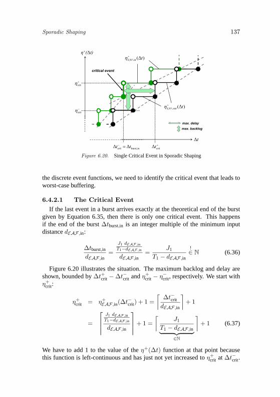
Sporadic Shaping 137
crit
crit
+( t)
t
max. delay
max. backlog
crittinburst,crit tt
critical event
)(in, tEAF
)(out, tEAF
Figure 6.20. Single Critical Event in Sporadic Shaping
the discrete event functions, we need to identify the critical event that leads toworst-case buffering.
6.4.2.1 The Critical EventIf the last event in a burst arrives exactly at the theoretical end of the burst
given by Equation 6.35, then there is only one critical event. This happensif the end of the burst ∆tburst,in is an integer multiple of the minimum inputdistance dEAF ,in:
∆tburst,in
dEAF ,in=
J1 dEAF,inT1−dEAF,in
dEAF ,in=
J1
T1 − dEAF ,in
!∈ N (6.36)
Figure 6.20 illustrates the situation. The maximum backlog and delay areshown, bounded by ∆t+crit − ∆t−crit and η+
crit − η−crit, respectively. We start withη+
crit:
η+crit = η+
EAF ,in(∆t−crit) + 1 =⌈
∆t−crit
dEAF ,in
⌉+ 1
=
⎡⎢⎢⎢
J1 dEAF,inT1−dEAF,in
dEAF ,in
⎤⎥⎥⎥+ 1 =
⌈J1
T1 − dEAF ,in︸ ︷︷ ︸∈N
⌉+ 1 (6.37)
We have to add 1 to the value of the η+(∆t) function at that point becausethis function is left-continuous and has just not yet increased to η+
crit at ∆t−crit.

138 Event Adaptation Functions
Calculating η−crit is straight-forward:
η−crit = η+EAF ,out(∆t−crit) =
⌈∆t−crit
dEAF ,out
⌉=
⎡⎢⎢⎢
J1 dEAF,inT1−dEAF,in
dEAF ,out
⎤⎥⎥⎥ (6.38)
We obtain as the maximum backlog:
backlog+EAF = η+
crit − η−crit
= 1 +⌈
J1
T1 − dEAF ,in︸ ︷︷ ︸∈N
⌉−⌈
J1
T1 − dEAF ,in
dEAF ,in
dEAF ,out
⌉(6.39)
To determine the maximum buffering delay, we calculate the delay betweenthe η+
critth input and output event:
delay+EAF = δ−EAF ,out(η
+crit) − δ−EAF ,in(η
+crit)
= (η+crit − 1)dEAF ,out − (η+
crit − 1)dEAF ,in
= (η+crit − 1)(dEAF ,out − dEAF ,in)
=⌈
∆tcrit
dEAF ,in
⌉(dEAF ,out − dEAF ,in)
=⌈
J1
T1 − dEAF ,in︸ ︷︷ ︸∈N
⌉(dEAF ,out − dEAF ,in) (6.40)
Equation 6.36 ensures that some of the rounded terms are integers and donot essentially need rounding. We have not further simplified this because thesame equations will be soon applied to other non-integer situations.
6.4.2.2 Two Critical Event CandidatesIf the last event in a burst does not exactly meet the end of the burst ∆tburst,in
given by Equation 6.35, then there are two candidates for the critical event, thelast event directly before and the first event directly after ∆tburst,in. Obviously,one of these events experiences the maximum backlog and delay, respectively.We therefore determine these properties for both events. The two candidatesare shown in Figure 6.21. We start by determining ∆tcrit,1 which is the largestinteger multiple of the minimum input distance dEAF ,in less than or equal to∆tburst,in:
∆tcrit,1 =⌊
∆tburst,in
dEAF ,in
⌋dEAF ,in (6.41)
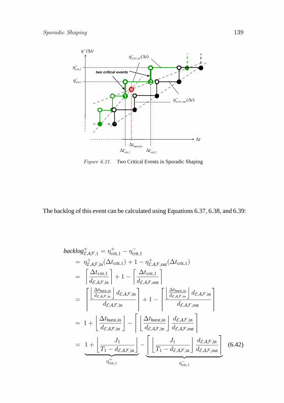
Sporadic Shaping 139
+( t)
t
crit,2tcrit,1t
2
1
two critical events
inburst,t
crit,2
crit,1
)(in, tEAF
)(out, tEAF
Figure 6.21. Two Critical Events in Sporadic Shaping
The backlog of this event can be calculated using Equations 6.37, 6.38, and 6.39:
backlog+EAF ,1 = η+
crit,1 − η−crit,1
= η+EAF ,in(∆tcrit,1) + 1 − η+
EAF ,out(∆tcrit,1)
=⌈
∆tcrit,1
dEAF ,in
⌉+ 1 −
⌈∆tcrit,1
dEAF ,out
⌉
=
⎡⎢⎢⎢⌊
∆tburst,indEAF,in
⌋dEAF ,in
dEAF ,in
⎤⎥⎥⎥+ 1 −
⎡⎢⎢⎢⌊
∆tburst,indEAF,in
⌋dEAF ,in
dEAF ,out
⎤⎥⎥⎥
= 1 +⌊
∆tburst,in
dEAF ,in
⌋−⌈⌊
∆tburst,in
dEAF ,in
⌋dEAF ,in
dEAF ,out
⌉
= 1 +⌊
J1
T1 − dEAF ,in
⌋︸ ︷︷ ︸
η+crit,1
−⌈⌊
J1
T1 − dEAF ,in
⌋dEAF ,in
dEAF ,out
⌉︸ ︷︷ ︸
η−crit,1
(6.42)

140 Event Adaptation Functions
The delay is obtained using Equation 6.40:
delay+EAF ,1 = δ−EAF ,out(η
+crit,1) − δ−EAF ,in(η
+crit,1)
= (η+crit,1 − 1)dEAF ,out − (η+
crit,1 − 1)dEAF ,in
= (η+crit,1 − 1)(dEAF ,out − dEAF ,in)
=⌊
J1
T1 − dEAF ,in
⌋(dEAF ,out − dEAF ,in) (6.43)
The arrival time of the second candidate can be determined similarly to thecalculation in Equation 6.41, but this time we are looking for the event arrivaltime greater than or equal to ∆tburst,in; and because the event arrives after theend of the burst, we need to consider a periodic behavior with jitter rather thana sporadic behavior with a minimum distance:
∆tcrit,2 =⌈
∆tburst,in
dEAF ,in
⌉T1 − J1 (6.44)
The backlog of this event is::
backlog+EAF ,2 = η+
crit,2 − η−crit,2
= η+EAF ,in(∆tcrit,2)︸ ︷︷ ︸
after end of input burst
+1 − η+EAF ,out(∆tcrit,2)︸ ︷︷ ︸
output still bursty
=⌈
∆tcrit,2 + J1
T1
⌉+ 1 −
⌈∆tcrit,2
dEAF ,out
⌉
= 1 +
⎡⎢⎢⎢⌈
∆tburst,indEAF,in
⌉T1 − J1 + J1
T1
⎤⎥⎥⎥−
⎡⎢⎢⎢⌈
∆tburst,indEAF,in
⌉T1 − J1
dEAF ,out
⎤⎥⎥⎥
= 1 +⌈
J1
T1 − dEAF ,in
⌉︸ ︷︷ ︸
η+crit,2
−⎡⎢⎢⎢⌈
J1T1−dEAF,in
⌉T1 − J1
dEAF ,out
⎤⎥⎥⎥︸ ︷︷ ︸
η−crit,2
(6.45)
The delay is obtained using Equation 6.40:
delay+EAF ,2 = δ−EAF ,out(η
+crit,2)︸ ︷︷ ︸
output still bursty
− δ−EAF ,in(η+crit,2)︸ ︷︷ ︸
after end of input burst
= (η+crit,2 − 1)dEAF ,out − (η+
crit,2 − 1)T1 − J1
= (η+crit,2 − 1)(dEAF ,out − T1) + J1
=⌈
J1
T1 − dEAF ,in
⌉(dEAF ,out − T1) + J1 (6.46)

Sporadic Shaping 141
task shaper exe. total buffer task total outputbacklog backlog buffer delay response delay jitter
T1 - 1 1 - 20 20 -T2 3 1 4 500 110 610 1120T3 - 1 1 - 150 150 110
Table 6.4. Experiment with Sporadic Shaper with a Time-Out of 200
Finally, we choose the larger value of both candidates:
backlog+EAF = max(backlog+
EAF ,1, backlog+EAF ,2)
= max
(1 +
⌊J1
T1 − dEAF ,in
⌋−⌈⌊
J1
T1 − dEAF ,in
⌋dEAF ,in
dEAF ,out
⌉,
1 +⌈
J1
T1 − dEAF ,in
⌉−⎡⎢⎢⎢⌈
J1T1−dEAF,in
⌉T1 − J1
dEAF ,out
⎤⎥⎥⎥)
(6.47)
delay+EAF = max( delay+
EAF ,1, delay+EAF ,2)
= max
( ⌊J1
T1 − dEAF ,in
⌋(dEAF ,out − dEAF ,in),
⌈J1
T1 − dEAF ,in
⌉(dEAF ,out − T1) + J1
)(6.48)
These are the general formulas for backlog and delay determination. Incase of single critical event, both values ∆tcrit,1 and ∆tcrit,2 are identical andthe general backlog calculations of Equation 6.47 can be reduced to those ofEquation 6.39. The same applies to the delay calculations
6.4.3 ExperimentsNow that we have derived a formal framework for sporadic shaping, we can
determine the properties of the initial example. Detailed results are given inTable 6.4. Compared to the solution with the periodic shaper (see Table 6.3),the required shaper buffer can be reduced from 4 to 3, and the buffering delayhas decreased from 1500 to 500, reducing the effective task T2 response timefrom 1610 to 610 time units. As a side-effect, the output jitter of task T2 couldnot be reduced.
In order to illustrate the application of sporadic shaping, we have varied thetime-out value of the shaper. The next experiments start with the maximum

142 Event Adaptation Functions
Figure 6.22. Scheduling Diagram of System Sporadic Shaper with a Time-Out of 400
task shaper exe. total buffer task total outputbacklog backlog buffer delay response delay jitter
T1 - 1 1 - 20 20 -T2 3 1 4 1100 110 1210 1120T3 - 1 1 - 150 150 110
Table 6.5. Experiment with Sporadic Shaper with a Time-Out of 400
possible time-out value, which is (see Equation 6.34) the original period of400 time units. Then we gradually decrease the time-out value to 140, andfinally 90 time-units. A detailed comparison shows the impact of shaping andthe trade-offs that provide room for optimizations.
6.4.3.1 400-Time Units ShaperWith a time-out of 400, we apply as much sporadic shaping as possible,
larger time-out values are not possible. The worst-case scheduling diagramis shown in Figure 6.22, again being identical to those with periodic shaping,and also to sporadic shaping with a time-out of 200. The reason is –again–the large minimum distance that prevents task T2 from re-arriving during theso called critical scheduling instant. Table 6.5 shows the detailed results ofthe experiment. While the periodic shaper required a buffer of size 4, themaximum required buffer size of the sporadic shaper is only 3, just as in thecase of a 200 time-unit time-out. The buffering delay is between the delays ofthe previous experiments.
6.4.3.2 140-Time Units ShaperA reduction of the time-out value below 150 time units results in more com-
plex worst-case scheduling diagrams, since now, re-activations of task T2 needbe considered during analysis. Figure 6.22 shows the worst-case schedulingdiagram.

Sporadic Shaping 143
Figure 6.23. Scheduling Diagram of System Sporadic Shaper with a Time-Out of 140
task shaper exe. total buffer task total outputbacklog backlog buffer delay response delay jitter
T1 - 1 1 - 20 20 -T2 3 1 4 320 110 430 1120T3 - 2 2 - 260 260 220
Table 6.6. Experiment with Sporadic Shaper with a Time-Out of 140
Task T2 re-arrives at t = 140 and preempts T3 which, in turn, re-arrivesat t = 200 before it has completed. Two more re-arrivals of T2 disturb theexecution of T3 further. Finally, the critical scheduling instant is finished at t =560. The figure shows that the response time of task T2 has not increased, sincethere is at most one preemption by T1. However, the lowest priority task T3 isnow being preempted more often than with larger time-out values. Hence, itsresponse time increases and even exceeds its own activation period, resultingin larger execution backlog. The detailed results are shown in Table 6.6.
We see that task T3 suffers from the decreasing time-out values, although therequired shaper buffer remains constant compared to the previous experiment.However, the buffering (or shaping) delay has further decreased from 500 to320.
6.4.3.3 90-Time Units ShaperIn the final experiment, we reduce the time-out to 90. The scheduling di-
agram in Figure 6.24 illustrates that the resulting scheduling is already verycomplex, again. There is almost no difference compared to the un-shaped ver-sion of Figure 6.16. Only the total input backlog of task T2 is now partitionedinto a shaping backlog of 2 and an execution backlog of 2, while the un-shapedversion requires an execution backlog of 4. The detailed results are shown inTable 6.7.

144 Event Adaptation Functions
Figure 6.24. Scheduling Diagram of System Sporadic Shaper with a Time-Out of 90
task shaper exe. total buffer task total outputbacklog backlog buffer delay response delay jitter
T1 - 1 1 - 20 20 -T2 2 2 4 170 150 320 1160T3 - 3 3 - 480 480 440
Table 6.7. Experiment with Sporadic Shaper with a Time-Out of 90
6.4.3.4 Experiment SummaryWe have seen that very large time-out values result in the same worst-case
scheduling as the periodic version with much less delay. In contrast, verysmall time-out values result in properties similar to the un-shaped version. Inthe middle range, there are interesting possibilities of optimizing the systemby trading buffering requirements against delays against output jitters, and theindividual task’s delays against each other. Figure 6.25 allows a direct com-parison of the worst-case scheduling scenarios of all experiments. The topscheduling diagram is taken from the experiment with a periodic shaper, theother diagrams illustrate the influence of decreasing time-out values from topto bottom. The bottom diagram shows the up-shaped version.
Table 6.8 provides the detailed results. The bold numbers represent optimalvalues for a specific property. We see that, in this experiment, each set-up isoptimal with respect to a particular property. This is not necessarily the case,as the fourth row of Table 6.8 already indicates. The sporadic shaper with atime-out of 140 shares the optimal task T2 backlog with four other solutionsand has non-optimal values for all other properties. However, it still representsa Pareto-optimal solution, since neither of the other solutions outperforms it inall properties. Usually, a higher number of time-out values results in a widerPareto front of sub-optimal solutions, which can be traded against each other.

Sporadic Shaping 145
periodic shaper
sporadic shaper 400
sporadic shaper 200
sporadic shaper 140
sporadic shaper 90
unshaped system
Figure 6.25. Scheduling Diagrams of All Experiments

146 Event Adaptation Functions
ShapingP 400 200 140 90 –
Accumulated Backlog(shaper + execution)
T1 1 1 1 1 1 1Ta
sk T2 5 4 4 4 4 4T3 1 1 1 2 3 3
Total 7 6 6 7 8 8
Accumulated Delay(shaper + response)
T1 20 20 20 20 20 20
Task T2 1610 1210 610 430 320 320
T3 150 150 150 260 480 480
Output JitterT1 - - - - - -
Task T2 20 1120 1120 1120 1160 1330
T3 110 110 110 220 440 440Table 6.8. Overview of Delay and Backlog of All Experiments
6.4.4 Shaping Sporadic StreamsSo far, we have applied shaping solely to periodic streams with jitter and
burst. Periodic shaping eliminates a jitter by re-synchronizing the events to theoriginal period, sporadic shaping reduces the strength of a burst by increasingthe minimum inter-arrival time between events. It is quite obvious that periodicshaping cannot be applied to sporadic streams, at least not in the way presentedin Section 6.2. But we can clearly apply sporadic shaping to sporadic streams.The same concepts that have been introduced also apply to sporadic shaping.The shaper’s output stream will then be:
SEAF ,out = SS+B(TEAF ,in, JEAF ,in, max(dEAF ,out, δ−EAF ,in(2)) (6.49)
The maximum backlog and delay calculation from Equations 6.47 and 6.48apply.
6.4.4.1 Maximum Sporadic ShapingThere is, however, an interesting situation that one could call “sporadic syn-
chronization”. If we choose the maximum allowed time-out value dEAF ,out,which is equal to the original sporadic period TEAF ,in, then the resulting streamis:
SEAF ,out = SS+B(TEAF ,in, JEAF ,in, TEAF ,in) (6.50)

Automatic Shaping 147
We can now apply the additional event model interface from Section 5.6.3 totransform that stream into a strictly sporadic (S) stream:
SEAF ,out = SS(TEAF ,in) (6.51)
In other words, under specific circumstances, we can apply a lossless eventmodel transformation:
EMIFS+B→S : {SS+B(T, J, d) ∈ EMS+B|d = T} �→ EMS
Starget = SS(Ttarget = Tsource) (6.52)
Together with a sporadic shaper, this interface allows sporadic streams to bevirtually re-synchronized to their original sporadic period. The standard cal-culations apply to the dimensioning of the shaper buffer and to obtaining theshaping delay.
6.5 Automatic ShapingSo far, we have considered shaping as a means to manually optimize schedul-
ing locally. There is, however, another very important application of shaping.We have seen in the previous chapter, that there exist situations, in which therequirement coverage test of Definition 5.4 fails, that compares the character-istic functions of a stream against the allowed range of the requirement. Inthese situations, no plain event model interface can be found. Shaping, how-ever, changes the specific parameters of a stream, along with the characteristicfunctions. Apparently, a given input stream Si,in can possibly be shaped suchthat the resulting stream meets a given input requirement Ri,in in cases whereno plain EMIF is available.
We have shown in Section 6.4.3 that the actual impact of shaping variesheavily with the choice of the shaper. Depending on the shaping type, periodicor sporadic, and on the time-out value, task activation can be deliberately con-trolled and optimized by the designer. In other words, designers can exploitalternatives when shaping streams. However, for an automatic procedure, thatwe will introduce in Chapter 7, we need a clear, unambiguous rule to select ashaper. Therefore, we first define appropriate goals of an automatic shaping.
We can distinguish optimizations from necessities as follows. A task’s inputrequirement must essentially be met, otherwise the task can not be analyzed.This is a necessity. When shaping cannot be avoided, we want to reduce the in-fluence of shaping on the overall system to a minimum, i. e. we are looking fora shaper with the minimum backlog and delay. In other words, the input streamshall be shaped as little as possible but as much as necessary. Everything be-yond these necessities can be subject to further user-controlled optimization,and is called user-controlled shaping.

148 Event Adaptation Functions
Definition 6.1. (Automatic Shaper)An Automatic Shaper EAF auto is a function that takes as argument an eventstream SEAF auto,in and a requirement R, and returns a shaped stream SEAF auto,out.
Let Z be the set of all possible event streams S, and P(Z) be its power set.Then, EAF auto is defined by:
EAF auto : Z × P(Z) �→ ZSEAF auto,out = EAF auto(SEAF auto,in,R) (6.53)
If possible, the function shapes the provided event stream such, that
a) the shaper’s output event stream is covered by the given requirement
RC(SEAF auto,out,R) = 1(true) , and (6.54)
b) the required amount of buffering and buffering delay is minimized. Thecorresponding parameters backlog+
EAF auto, backlog−EAF auto
, delay+EAF auto
, anddelay−EAF auto
are associated with the Automatic Shaper.
If there exists no shaper that fulfills the given requirement R according toEquation 6.54, the function returns the un-shaped source stream, and the fourparameters have a value of zero (0).
The experiments of Section 6.4.3 have shown us that sporadic shaping hasa smaller influence than periodic shaping, and that smaller possible time-outvalues result in less buffering and less delay. Hence, sporadic shapers are fa-vored over periodic shapers for automatic shaping. Furthermore, an automaticshaper must have the minimum possible time-out value that is just sufficient tomeet the input requirement with respect to the allowed minimum event distanceδ−. The minimum possible value is taken from all allowed streams (Ri,in) thatsupport the actual input period and the actual input jitter:
dEAF auto,out = minS∈{Sx∈Ri,in|Tx=Ti,in∧Jx≥Ji,in}
(δ−S (2)) ≤ δ−Si,in(2) (6.55)
Practically speaking, the minimum time-out value must be selected accordingto the maximum allowed transient input frequency, given that the period andthe jitter are within the allowed range.
We have mentioned in Section 6.4.1 that sporadic shaping never reduces thejitter, it can only reduce transient event frequencies. In case the input jitterexceeds the maximum allowed jitter, then the set
{Sx ∈ Ri,in|Tx = Ti,in ∧ Jx ≥ Ji,in}is empty, and no appropriate dEAF auto,out can be found using Equation 6.55.There is one exception, which we called maximum sporadic shaping in Sec-tion 6.4.4. This eliminates the jitter of a sporadic stream by choosing the max-imum possible timeout value, which is the sporadic period TS of the stream.

Polling 149
T1T4
S4,data=S1,out
S4,act=SP(T4,act)
S4,out=?
R4=?
backlog4,data=?
delay4,data=?
Figure 6.26. Periodic Polling Task and the Involved Event Streams
In case of the input stream is periodic with a too large jitter, a periodic shaperof Section 6.2 must be used. In the introductory example of this chapter, wehave shown that the original period of the stream must be clearly compatiblewith the task input requirement (see Equation 6.4).
6.6 PollingIn Section 6.2, we have shown how periodic streams can be re-synchronized
to their original period. An experiment has shown how such periodic shaperscan result in a periodic execution of an otherwise very dynamic task, therebysubstantially reducing peak loads and increasing the determinism.
Periodic task execution, however, does not necessarily always require strictlyperiodic inputs. Polling is a popular mechanism to also apply periodic execu-tion to asynchronous inputs, including sporadic streams. The behavior of apolling task is influenced by two event streams. A strictly periodic one thatactivates the task, and another arbitrary one that influences the tasks functionalbehavior. Figure 6.26 shows a polling task T4 and the two streams, one acti-vating event stream S4,act and one data stream S4,data coming from task T1.
In other words, the activation scheme does not reflect communication andvice versa. Rather, a polling task is not activated upon the availability of inputsbut is time-driven. When activated, then it tests its inputs for available data,and the task’s behavior might further depend on the success or failure of thetest.
There are four parameters that must be determined, as illustrated in Fig-ure 6.26. The buffer is needed to synchronize the data input to the periodicexecution, and we need to determine the data buffering delay delay+
4,data and
backlog backlog+4,data. Furthermore, the execution delay, i. e. the response time

150 Event Adaptation Functions
0
( t)
1
2
3
4
5
t
delaybacklog
1
act4 )(T
tt
,
)()( out1,data4, tt
6
Figure 6.27. Polling a Periodic Stream with Burst
R4,data, is required to finally determine the output stream S4,out of the pollingtasks.
6.6.1 Input BufferA task that periodically polls its input, implicitly performs shaping on the
input stream. When both sender and receiver have the same period, pollingcorresponds to periodic shaping introduced in Section 6.2. Depending on thepossible jitter or burst, it requires buffering and induces a delay, and the back-log and delay calculations from Equations 6.32 and 6.31 can be re-used. Suchperiodic task activation is often found in systems with loosely coupled taskcommunication. The buffer synchronizes tasks which run independent sched-ules but still share a common periodicity or frequency as part of their combinedfunction, e. g. in distributed filter functions.
When the timing of the receiver (its period) is nearly independent of the in-put data, the situation resembles key characteristics of sporadic shaping. Sim-ilar to condition 6.34, the polling task must be at least as fast as the input dataarrives on stream S4,data to prevent buffer overflows:
T4,in ≥ T4,act (6.56)
This requirement is based on the assumption that each input must essentiallybe read by the polling task. However, there are applications where this is notnecessarily required. Simulink [115], for instance, defines periodic tasks thatcommunicate through registers, and data can eventually be overwritten beforeit is read. This eliminates causal relations between event arrival and task execu-tion. We have thoroughly analyzed the importance of register communication

Polling 151
and non-causal task execution in our SPI project (see Section 2.4). This thesis,however, focuses on causal performance dependencies, and register communi-cation is not considered further.
The event curves of Figure 6.27 illustrate a polling scenario with bursts onthe data input stream S4,data. The behavior in the case of polling is very similarto the behavior known from sporadic burst reduction, as introduced in Sec-tion 6.4.1. Hence, similar calculations can be applied. There is, however, akey difference. While shapers consume an input event as early as possible, apolling task must be assumed to read the input as late as possible, because itis executed independently of the input stream timing. In other words, an inputevent unusually has to wait until the next activation of the polling receiver. Thisadds a constant amount of time to the overall delay, and also affects buffering.
We can determine the end of the input burst and the corresponding two crit-ical events using the known Equations 6.41 and 6.44 with some modifications.In Equations 6.47 and 6.48, we
substitute the time-out value dEAF ,out with the polling period T4,act,
use the more general δ−1 (2) instead of dEAF ,in to allow the application tojittery streams without burst, and
add one activation period T4,act to the delay to account for the possible“late” consumption of the receiver
We obtain:
backlog+4,in = max
(1 +
⌊J1
T1 − δ−1 (2)
⌋−⌈⌊
J1
T1 − δ−1 (2)
⌋δ−1 (2)T4,act
⌉,
1 +⌈
J1
T1 − δ−1 (2)
⌉−
⎡⎢⎢⎢⎢⌈
J1
T1−δ−1 (2)
⌉T1 − J1
T4,act
⎤⎥⎥⎥⎥)
(6.57)
delay+4,in = T4,act + max
( ⌊J1
T1 − δ−1 (2)
⌋(T4,act − δ−1 (2)),
⌈J1
T1 − δ−1 (2)
⌉(T4,act − T1) + J1
)(6.58)
6.6.2 Execution Load and Response TimeThe activation of the polling task is fully independent of the actual data in-
put. Hence, scheduling analysis only needs to consider the activating event

152 Event Adaptation Functions
stream S4,act. The execution time, which may be data-dependent, can be cap-tured by an execution time interval. Scheduling analysis will then provide acorresponding response time interval and the minimum and maximum load.The details of the actual scheduling analysis are not in the key focus of thisthesis. Rather, this work focuses on the amount of information required to en-able the analysis. We see that the data input stream S4,data is not essentiallyneeded.
There are, however, scheduling analysis techniques that can distinguish be-tween several execution behaviors or contexts [55]. For such techniques, theinput stream S4,data provides important information about the distribution ofthe two distinctive behaviors.
6.6.3 Output Event StreamsTo determine the output stream, we have to know about the implementation
of the polling task. There are two possible (and equally popular) ways to im-plement the output communication. One possibility is to always produce anoutput event and to code the success of the poll, or other state information,in the produced data. Such implementations are found in periodic data-flowimplementations as generated by Simulink [115]. In this case, the situationcan be reduced to a periodically activated task that always produces an outputevent, and the output calculations from Section 4.1 apply:
S4,out = SP+B
(T4,out = T4,act,
J4,out = J4,R = R+4 − R−
4 ,
d4,out = max(T4,act − J4,R, R−
4
) )(6.59)
The second possibility is to only produce an output event after a successfulinput poll, i. e. if a data input was available from stream S4,data. In other words,the task has a conditional output production. According to Section 4.5, suchtasks produce their output sporadically. So we can directly re-use all calcula-tions from Equation 6.59 but simply have to change the event model class fromperiodic into sporadic.
However, this procedure yields an overly conservative bound on the realoutput stream behavior. The polling task does not behave randomly but reactsto the availability of data on stream S4,data, and the actual input-output behavioris in fact deterministic. In other words, key properties of the input stream willbe propagated to the output, such as an average period:
T4,out = T4,data = T1 (6.60)
We can account for this input-output relationship when we consider the en-tire path from task T1 to the output of task T4. Figure 6.28 illustrates this. We

Polling 153
T1T4
S4,data=S1,out=SP+ (T1,J1,d1)
S4,act=SP(T4,act)
S4,out=SP+ (T4,out=T1, J4,out=?, d4,out=?)
R4delay4,data
RpollFigure 6.28. Output Stream of Conditional-Output Polling Tasks
determine the combined response time of the input buffer and the task execu-tion:
Rpoll = delay4,in + R4
R+poll = delay+
4,in + R+4
R−poll = delay−4,in + R−
4
Jpoll = R+poll − R−
poll
Now, we apply this combined response time to the input stream of task T4 andwe obtain as output:
S4,out = SP+B
(T4,out = T1,
J4,out = J1 + Jpoll,R,
d4,out = max(T1 − Jpoll, R
−4
) )(6.61)
We can even incorporate key information about the activation period of taskT4 to further tighten the minimum output distance d4,out by using the maximumvalue of both Equations 6.59 and 6.61:
d4,out = max(T1 − Jpoll, T4,act − J4,R, R−
4
)(6.62)
This is specifically useful, if the input stream is bursty and the bufferingdelay exceeds the original period. This optimization accounts for the fact that
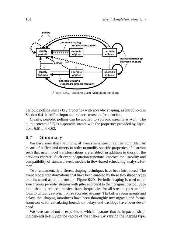
154 Event Adaptation Functions
strictly
periodic
periodic
w/ jitter
periodic
w/ burst
strictly
sporadic
sporadic
w/ jitter
sporadic
w/ burst
burst reduction by
sporadic shaping
sporadic shaping
("sporadic synchronization")
periodic shaping /
re- synchronization
polling
polling
Figure 6.29. Existing Event Adaptation Functions
periodic polling shares key properties with sporadic shaping, as introduced inSection 6.4. It buffers input and reduces transient frequencies.
Clearly, periodic polling can be applied to sporadic streams as well. Theoutput stream of T4 is a sporadic stream with the properties provided by Equa-tions 6.61 and 6.62.
6.7 SummaryWe have seen that the timing of events in a stream can be controlled by
means of buffers and timers in order to modify specific properties of a streamsuch that new model transformations are enabled, in addition to those of theprevious chapter. Such event adaptation functions improve the usability andcompatibility of standard event models in flow-based scheduling analysis fur-ther.
Two fundamentally different shaping techniques have been introduced. Theevent model transformations that have been enabled by these two shaper typesare illustrated as bold arrows in Figure 6.29. Periodic shaping is used to re-synchronize periodic streams with jitter and burst to their original period. Spo-radic shaping reduces transient burst frequencies for all stream types, and al-lows to virtually re-synchronize sporadic streams. The buffer requirements anddelays that shaping introduces have been thoroughly investigated and formalframeworks for calculating bounds on delays and backlogs have been devel-oped.
We have carried out an experiment, which illustrates that the impact of shap-ing depends heavily on the choice of the shaper. By varying the shaping type,

Summary 155
periodic or sporadic, and the time-out value, designers can deliberately controland optimize the system behavior. We call such optimizations user-controlledshaping that we distinguish from automatic shaping, which allows the system-atic reduction of shaping backlogs and delays, whilst still meeting given inputrequirements.
Finally, we have analyzed the situation of input polling. Polling is basi-cally an implementation choice for a task rather than an operation on an eventstream. The influence of polling on buffers and event timing, however, isstrongly related to shaping. Depending on the specific situation, polling canbe formally seen as either type of shaping, and the derived formal frameworkallows calculation of buffer sizes and delays also for systems with polling. Wehave shown that, and how, the event stream view helps to optimize the outputstream accuracy in the presence of polling.


Chapter 7
SYSTEM-LEVEL ANALYSIS PROCEDURE
Each of the four preceding chapters provides one important concept thatlets us a) capture component inputs and task activation as a pre-requisite forscheduling analysis, b) model and provide a relation between inputs and out-puts of a task or a component, influenced by scheduling and execution, c) pro-vide appropriate event model interfaces to match the analysis requirements,and d) apply appropriate event stream adaptation to facilitate the interfacingstep (or to optimize the scheduling).
These concepts cover the key local aspects of scheduling and response timeanalysis in a system-level context. This chapter integrates these individual con-cepts and uses them as hand tools to apply the flow-based analysis approach,as introduced in Section 2.3, to systems with multiple heterogeneous eventmodels.
We start with a brief review of the introduced formalisms and define an ap-propriate system analysis model. In order to extend the iterative flow-basedapproaches from Thiele [116] and Gresser [38, 39] to support heterogeneousevent models, we have to insert an appropriate event model interfacing step.We will see that these interfaces not only enable this new analysis procedure,but that adaptations also allow control of the streams during the analysis andintegration process, and to globally optimize the system. This is of particu-lar importance in systems where the mixture of architectural and functionalinfluences leads to complex and confusing cyclic dependencies and schedul-ing anomalies. These can turn the iterative analysis into a convergence prob-lem, and we identify monotonicity properties to formulate termination condi-tions. We show how bottlenecks and pitfalls can be identified, resolved, andoptimized using this new analysis procedure. We use expressive examples todemonstrate the individual steps as well as the overall analysis.

158 System-Level Analysis Procedure
T1
T2
(C1,P1)
T3
(C3,P3)(C2,P2)
CPU1
S1,out
S2,in
S3,in
S1,4
S3,5
R1
R2
R3
TX
SX,out=SX,1=S1,in
T6
BUS2
T5
(C4,P4)
(C6,P6)(C5,P5)
R4
R5
R6
T4 TY
S4,out=S4,Y=SY,in
T8
BUS2
T7
CPU2
T9
T6
(C7,P7)
R7
Figure 7.1. System Model Example
7.1 System Analysis ModelWe summarize the required elements, parameters, and the overall structure
using part of an example system as illustrated in Figure 7.1.
7.1.1 Model Elements and ParametersThe system consist of a set of tasks Ti. Each task Ti is mapped to a resource
RSCj and is scheduled there according to the resource’s scheduling strategy.Each task has two mapping-specific parameters: the core task time Ci and thescheduling parameters Pi. We do not further distinguish between computationtasks (processes) and communication tasks (channels, links, etc.). Both requirea net resource access time (Ci). The actual response time Ri defines the timebetween the occurrence of the request (activation time) and the time this re-quest has been successfully served (completion). Both the core task time andthe response time are intervals with upper and lower bounds.
7.1.2 Model Structure and DependenciesThe response time Ri abstracts from the detailed scheduling influences that
task Ti experiences due to e. g. preemptions by other tasks. It represents thetasks externally observable execution or communication timing behavior. Theinteraction with other tasks is captured using event streams: an input event

The System-Level Analysis Procedure 159
stream Si,in and an output event stream Si,out. Through these uni-directionalstreams, tasks communicate with each other. The output stream Si,out of taskTi becomes the input stream Sk,in of task Tk, the stream itself is denoted Si,k.Each task must have exactly one input stream, while a task’s output can beconnected to several task’s inputs. In the example of Figure 7.1, the output ofT1 is connected to two tasks, T7 and T4, respectively. This allows task trees tobe captured.
7.1.3 Environment ModelingTasks TX and TY are environmental tasks that model timing constraints and
assertions of the environment that the system is embedded in. Task TX is anenvironmental source task that provides information about the timing of theprimary inputs to the system, such as an actuator connected to CPU1. TY isan environmental sink task that also has a certain timing behavior represent-ing a timing constraint, such as a maximum bound on the allowed jitter or amaximum sporadic period. Using event streams and models, not only withinthe system but also between the system and its environment, we can elegantlymodel environmental assertions and constraints without requiring additionalconcepts.
7.1.4 Local SchedulingThe event streams are the key integrating elements in this proposed analysis
approach. Each resource RSCj has one local analysis method associated thatcalculates the response time Ri of the tasks as reviewed in Section 2.1. Theanalysis takes as input the following parameters of each task Ti mapped on thatresource: the core task time Ci, the scheduling parameter Pi, and the activatingevent stream Si,act.
The analysis requires the activating stream to comply with an analysis-dependent input event model requirement Rj,in as introduced in Chapter 5. Inorder to meet this requirement, the actual input stream Si,in might need to beappropriately transformed by means of event model interface and/or automaticshapers as introduced in Chapters 5 and 6.
After analyzing the scheduling, the output event stream Si,out is determinedfrom the input stream and the response time using a function O(Ri,Si,in). Wethoroughly discussed the dependencies between response times and input andoutput streams in Chapter 4.
7.2 The System-Level Analysis ProcedureFigure 7.2 provides an abstract view of the overall system-level analysis
procedure consisting of 7 steps and a set-up step (step 0). The overall ideaof iterative event stream propagation is not fully new, it has been proposed

160 System-Level Analysis Procedure
FAILED!
no
no
derive output event streams
can input be captured?
choose analyzable resource
propagate streams globally
capture primary system inputs0
1
2
4
5
constraints met ?6
all resources analyzed ?7no
yes
SUCCESS!
yes
yes
resource schedulable ?no
yes
3
Figure 7.2. System-Level Analysis Procedure
by Gresser [38, 39] and Thiele et. al. [116]. The novelty of our approach isthat is allows the use of known local analysis techniques, that possibly requireheterogeneous event models, enabled by event model interfacing and streamadaptation.
Step 0: Capturing Primary System InputsThe primary system inputs are represented as environmental source tasks. Weintroduced environmental modeling in Section 7.1.3. The environment speci-fication determines the input event streams of the directly connected tasks:
∀Sa,b, a ∈ {Tenv} : Sb,in = Sa,out (7.1)
Step 1: Choosing an Analyzable ResourceScheduling analysis requires the activation of all tasks to be known. Hence, wecan only analyze a resource when the activating event streams are known, inturn requiring that the input streams are known for all tasks on that resource.In the beginning, these are usually the ones which are connected to the primarysystem inputs.
Step 2: Capturing Task ActivationAfter selecting a resource for analysis, we have to capture the activation of alltasks in a way suitable for the analysis. This might impose an analysis-specific

The System-Level Analysis Procedure 161
can input be captured?input
requirement
met?
exists
appropriate
EMIF?
insert EMIF
no
exists
appropriate
EAF?
no
no
possibly insert additional shaper for optimization purposes
yes
yes
yes
insert minimum shaper
2
Figure 7.3. Input Event Stream Capturing
input model requirement Ri,in on the task input streams. Depending on thesituation, this step might incorporate several sub-steps illustrated in Figure 7.3.We have to apply the procedure to each task separately.
We start with testing whether the input stream meets the requirement (seeSection 5.2):
Si,in?∈ Ri,in (7.2)
If the test is successful, the input stream already represents the activatingstream that can be used for scheduling analysis (in step 3):
Si,act = Si,in (7.3)
If test 7.2 fails, we look for an event model interface that transforms the in-put stream representation into a representation suitable for analysis. We applythe requirement coverage test from Definition 5.4:
RC(Si,in,Ri,in)!= 1 (true) (7.4)
If the test is successful, we can insert the appropriate EMIFs introduced inChapter 5 to transform the input stream into an activating stream that meets theinput requirement:
Si,act = EMIFEMi,in→EMi,req(Si,in) ∈ Ri,in (7.5)

162 System-Level Analysis Procedure
If also test 7.4 fails, we try inserting an automatic shaper (see Definition 6.1),that reduces too high transient loads or fully eliminates jitters. Then, we checkif the resulting shaped stream meets the input requirement, possibly with anadditional EMIF :
Si,shaped = EAF auto(Si,in,Ri,in)
RC(Si,shaped,Ri,in)!= 1(true)
When even automatic shaping does not help, the input stream can simply notbe reasonably transformed into the required representation. In effect, (at leastsome of) the tasks on that resource will not be analyzable by the next step, andwe can terminate the iterative analysis procedure. There are two classes of rea-sons for such failures: First, to prevent inputs that lead to permanent overload,a task might have a minimum allowed average period, reflecting a maximumaverage execution frequency. Input streams that have a smaller average periodare not acceptable. Second, there might be a general mismatch between the in-tended behavior of the producer task and the consumer task, for instance bothhave different periods but were assumed to execute in strong relationship witheach other. Either source of failure represents a well-known system integrationproblem. The event stream view implicitly detects such integration problems.
In case of a successful activation modeling, i. e. all input streams can betransformed to meet the corresponding task input requirements, a user mightconsider additional local optimizations using periodic or sporadic shaping. Wehave shown the impact of such user-controlled shaping in Section 6.4.3. A spe-cial case where such local optimizations help to globally increase the schedu-lability of the system, is discussed in Section 7.7.
Step 3: Local Scheduling AnalysisWhen all task activation models are known from the previous step, the schedul-ing on the selected resource can be analyzed. For local scheduling analysis, abig variety of techniques is available from the real-time systems community.We reviewed popular techniques and landmark publications in Section 2.1. Inaddition to the task activation models, these techniques require the core execu-tion time Ci as well as the scheduling parameters Pi of each task to be known.The scheduling analysis returns the response time Ri of each task which deter-mines the externally observable timing behavior of a task.
This is the second step of the overall procedure that can fail. An exampleis a permanent overload situation that clearly makes some, if not all tasks un-schedulable. Less obvious examples are situations where the system is in factschedulable but the analysis has limitations that prevent it from calculating abounded response time. The initial proposal for rate-monotonic analysis [73]

Local and Global Constraint Verification 163
is such an example. Response times larger than periods are just not considered.In either case, the local analysis cannot determine a response time for a subsetof tasks. Again, the systematic procedure and the event stream view help inidentifying a potential modeling insufficiency or a performance bottleneck.
Step 4: Determining the Output StreamsWe have shown in Chapter 4 that the output stream is a function of the inputstream and the response time:
Si,out = O(Si,in, Ri)
If available, additional information about the implementation of a task, forinstance polling characteristics (see Section 6.6), can further tighten the outputstream calculations.
Step 5: Propagating Event Streams GloballyIn this step, the just obtained output streams are propagated to the inputs of theconnected tasks in the application:
Sk,in = Si,out
Step 6: Constraint VerificationWhen all tasks have been successfully analyzed, the system is schedulable,in general meaning that no permanent overload conditions occurred, and wecan check if the given constraints are met. We have already mentioned thatenvironmental sink tasks can be used to model constraints on event steamsthat enter the environment, and there is a variety of additional possibilities toverify other system properties such as local deadlines, buffer constraints andpath latencies, which we explain in Section 7.3. If one of these constraints isviolated, the analysis can be aborted.
Step 7: IterationNow, the whole process iterates from the beginning. During the iteration, eventstreams are propagated through the system of locally analyzable components,from the primary system inputs to the system outputs, i. e. to the environmentalsink tasks. The iteration is successfully completed when all resources havebeen analyzed, and fails if either not all task inputs could be appropriatelytransformed to meet requirements, or a bounded response time could not bedetermined for all tasks, or another constraint is violated.

164 System-Level Analysis Procedure
7.3 Local and Global Constraint Verification7.3.1 Environmental Constraints
A dedicated period and a maximum allowed jitter at the interface betweenthe system outputs and the environment is a popular example for an environ-mental constraint. It can be elegantly modeled using a virtual sink task with anappropriate input requirement:
Rsink,in = {SP+J ∈ EMP+J|T = Tsink, J ≤ Jsink}
As another example, a maximum allowed frequency can be modeled using asporadic input requirement. As they use virtually the same modeling concepts,the environmental source and sink tasks can be included in the analysis proce-dure, and the requirements are automatically checked during step 2. Moreover,stream transformation using EMIFs and EAFs is considered representing anautomatic output adaptation. However, in our examples later, this particularcheck is delayed and considered after the system has been fully analyzed.
7.3.2 Internal Event StreamsThe event streams capture in detail the interaction between tasks and pro-
vide information about the resource access patterns of individual tasks. Theadditional delays and the buffer memory that is required because of shapingallows the impact of such shaping decisions on the overall system timing andperformance to be determined.
7.3.3 Local Task and Resource PropertiesThe local response times as a direct result from the individual task schedul-
ing analysis allow the actual execution timing to be checked against the ex-pected timing and/or local constraints such as a deadline. It furthermore pro-vides information about each individual task’s performance for a given map-ping of tasks to resources.
The total load or utilization of each resource in the system allows the iden-tification of bottlenecks, as well as the remaining performance in the architec-ture. In practice, this can be of particular importance for selecting components(resources) to be optimized in terms of speed and performance, e. g. bus band-width.
7.3.4 Path ConstraintsFrom the mentioned local timing properties we can determine key global
timing and performance properties. Very often, it is not the individual tasks thatare constrained to exhibit a certain timing behavior. Rather, the interactions ofseveral tasks form a system function that is required to meet a certain deadline.

Local and Global Constraint Verification 165
TX
S1,EAF
T2
R2
S2,3T3
R3
SX,1T1
R1
TY
S3,YSEAF,2
delayEAF
PL1=R1+delayEAF
PC1
PL2=R1+delayEAF
+R2+R3 PC2
!
!
P1={T1,EAF}
P2={T1,EAF,T2,T3,}
Figure 7.4. Path Latencies and Constraints
Such system functions usually span a whole path from primary system inputsto primary system outputs, including several tasks and event streams.
Definition 7.1. (Path)A path Pi is a connected set of tasks, shapers, and event streams. A path musthave a dedicated starting element, and a termination element, and at most oneoutput event stream of each task can be included in that path, prohibiting a pathfrom containing branches.
Definition 7.2. (Path Constraint)A Path Constraint PCi is a positive real that bounds the allowed maximum
time each event requires to travel along that path Pi.
To check the compliance with such path constraints, we need to determinethe actual path latency or path delay by accumulating the delays of the individ-ual path elements.
Definition 7.3. (Path Latency)The accumulated task response times and shaping delays of all elements in a
path Pi yield the Path Latency PLi:
PLi =∑Tj∈Pi
RTj +∑
EAFk∈Pi
delayEAFk(7.6)
The path latency is an interval, and the upper and lower bounds are determinedby accumulating the corresponding upper and lower bounds of the responsetimes and shaping delays.
Figure 7.4 shows three system tasks, one sink and one source task, and oneshaper, which are connected as a path with five event streams. Two pathsP1 and P2 are shown together with their respective latencies. These paths

166 System-Level Analysis Procedure
represent chains in the application and could possibly be specified by theirstart and end node –task or shaper. Other work allows also functional cycles tobe included in a path [140, 52], that are not considered further here.
7.3.5 Buffer ConstraintsThe execution backlog of all tasks on one resource determines (together
with the “size” of the data that the events might carry) the total required in-put buffers which might be constrained because of limited memory for thatresource. Likewise, the shaping backlog of all elements provides the memoryrequired for shaping. We mentioned that such shaping can be elegantly doneby operating system functions or hardware drivers that adds to the overall re-quired memory. The required execution and shaping backlogs along a pathalso provide interesting information about the “bottleneck distribution” alonga path.
7.4 Cyclic Event Stream DependenciesSo far, we have assumed that we can always find a resource with all input
streams known in each analysis iteration (step 1). Unfortunately, this is notnecessarily the case. Recall the example system from the introduction. Wehighlighted a non-functional dependency cycle in Figure 1.5. The two keycomponents, the CPU and the bus, are mutually dependent on each other withrespect to the event streams. Each resource requires an output stream of theother one to be known before it can be analyzed. In such situations the primarysystem inputs do not provide a starting point for the analysis procedure ofSection 7.2, since no resource has all input streams known.
It is important to recognize that such dependency cycles can turn the itera-tive analysis procedure into a convergence problem as illustrated in Figure 7.5,and we are facing two key challenges: We have to find a reasonable start-ing point for the iterative procedure and we have to guarantee convergence, orfind a reasonable termination condition. The detailed analysis of the impactof scheduling and execution on output event streams in Chapter 4 provides uswith a basic approach.
7.4.1 The Starting PointWe know that execution and scheduling adds jitter characteristics to event
streams from task inputs to task outputs, i. e. the jitter grows from input tooutput at each local analysis while the original input period is preserved at theoutput, regardless whether periodic or sporadic. We can exploit this behaviorand start the actual analysis procedure by propagating all input streams fromthe primary system inputs through the system without considering the influenceof scheduling. In other words, we simply “copy” the input stream of a task to
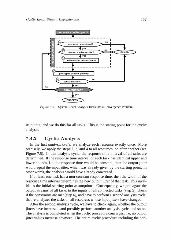
Cyclic Event Stream Dependencies 167
for
each
reso
urc
e
no
generate starting point
FAILED!
no
derive output event streams
can input be captured?2
4
yes
resource schedulable ?no
yes
3
no
propagate streams globally5
constraints met ?6
yes
SUCCESS!
yes
convergence?
Figure 7.5. System-Level Analysis Turns into a Convergence Problem
its output, and we do this for all tasks. This is the stating point for the cyclicanalysis.
7.4.2 Cyclic AnalysisIn the first analysis cycle, we analyze each resource exactly once. More
precisely, we apply the steps 2, 3, and 4 to all resources, on after another (seeFigure 7.5). In that analysis cycle, the response time interval of all tasks aredetermined. If the response time interval of each task has identical upper andlower bounds, i. e. the response time would be constant, then the output jitterwould equal the input jitter, which was already given by the starting point. Inother words, the analysis would have already converged.
If at least one task has a non-constant response time, then the width of theresponse time interval determines the new output jitter of that task. This inval-idates the initial starting-point assumptions. Consequently, we propagate theoutput streams of all tasks to the inputs of all connected tasks (step 5), checkif the constraints are met (step 6), and have to perform a second analysis cycle,that re-analyzes the tasks on all resources whose input jitters have changed.
After the second analysis cycle, we have to check again, whether the outputjitters have increased, and possibly perform another analysis cycle, and so on.The analysis is completed when the cyclic procedure converges, i. e. no outputjitter values increase anymore. The entire cyclic procedure including the con-

168 System-Level Analysis Procedure
vergence test is illustrated in Figure 7.5. The important question is: Does theanalysis converge, and when?
7.4.3 Convergence and TerminationWhen we take a closer look on the consequences of increasing input jitter
of a task, we can distinguish two effects. First, the output jitter of that taskwill also increase because of the jitter inheritance phenomenon, that we men-tioned in Section 4.1.3. This inheritance applies to all tasks along paths inthe system. The second effect of increasing input jitters is scheduling distor-tion. An increasing input jitter distorts the scheduling and potentially increasesthe amount of worst-case interference, consequently increasing worst-case re-sponse times. Conversely, the best-case response times decrease, finally re-sulting in larger output jitters. This also shows that our initial assumption isvalid, since the initial input streams with smaller jitters are covered by all laterinput streams with a possibly larger jitter. In other words, the initially assumedsystem behavior is still included in the possible behavior of all later steps.
Convergence criteria and the actual time-complexity of the entire analysis,however, are extremely complex to determine, even though we know the influ-ences that let jitters and response times increase. We could at best bound thenumber of analysis cycles, but the overall complexity also depends stronglyon the complexity of the local analysis algorithms. These are embedded inthe global cyclic analysis procedure and could possibly pose further questionsto numerical convergence and stability. The holistic analysis approach (seeSection 2.2.2), that seeks an iterative solution of a complex set of recursivesystem-level timing equations, is faced with a comparable convergence prob-lem. This, however, has not even been solved there, although many groupscontinuously extend and enhance the related holistic equations and algorithms.In this thesis, we will not investigate this issue further, since we can formulatea reasonable termination condition that allows the efficient application of thecyclic analysis procedure in practice.
We know that, in case of fixed-priority scheduling, the interference of a taskis the sum of integer multiples of the core execution time of other tasks on thesame resource (see Equation 3.22). Likewise, in time-driven scheduling, theinterference is an integer multiple of one or more slot times (see Equation 2.9),etc.. Consequently, the amount of interference can only increase in discretesteps; and the minimum increment is bounded by, for instance, the minimumcore execution time, the smallest slot time, or the execution time of some oper-ating system function. In effect, the response times and the output jitters of atleast some tasks will monotonically grow with a minimum “speed”. This mini-mum speed prevents the jitters and response times from asymptotic expansion.Sooner or later, the analysis will either successfully converge, or a constraintwill be violated, and the analysis can be safely terminated. This lets us bound

Example 169
EAF3
EAF2
EAF1
M2DSPIP2M3IP1
HW
M1CPU
Sens
sporadic
w/ jitter
C1
C3bus
C2
periodic
w/ burst
periodic
w/ jitter
simple
sporadic
periodic
simple
periodic
T3T1
fmax=1,7kHz, s=8kB
f=140kHz, s=1kB
f=20kHz
s=3kB
8kB 32 ( 256 + 6 ) byte
1kB 1 ( 1024 + 6 ) byte
3kB 24 ( 128 + 6 ) byte
simple
sporadic
periodic
periodic
w/ burst
Figure 7.6. Detailed System Example
the number of analysis cycles from the given deadlines, path constraints, en-vironmental sink constraints, and task input requirements. As an additionaladvantage, the global solution procedure proposed tightly follows the event-and data-flow in the system. This makes the cyclic analysis, especially withrespect to convergence issues, easily comprehensible.
7.5 ExampleNow, we demonstrate the applicability of the approach by fully analyzing
the example from the introduction (see Figure 1.2) where we have integratedtwo functionally independent sub-systems using a shared bus. The CPU sub-system consists of a sensor that eventually sends data that must be processedby the CPU. In turn, the CPU accesses a hardware accelerator (HW). The DSPsub-system runs a highly optimized digital signal processing application andthe communication over the bus is critical. We have highlighted the key analy-sis challenges in Section 1.1 including cyclic dependencies and model incom-patibilities.
7.5.1 System Set-UpFigure 7.6 provides a detailed view on the entire system. The individual
components are now specified.

170 System-Level Analysis Procedure
7.5.1.1 The Primary System InputsThere are three inputs to the system: The sensor sporadically sends data
blocks of 8kb size to task T1, with a maximum sending frequency of 1, 7kHz,which corresponds to a sporadic event model with a minimum sporadic periodof 1
1,7kHz = 588µs. Task T3 is periodically activated by an RTOS (real-time
operating system) timer on the CPU with a period of 120kHz = 50µs. The high-
performance DSP application on the IP1 component has a sending frequencyof 140kHz, corresponding to a period of 7, 14µs.
These inputs are modeled as environmental source tasks. The formal eventstream definitions are:
Ssens = SS(Tsens = 588.2)Stimer = SP(Ttimer = 50)SIP = SP(TIP = 7.14)
7.5.1.2 The Bus TimingThe communication over the bus is implemented using a non-preemptive
static priority protocol. Instead of sending the complete data blocks as a sin-gle transmission, the data is fragmented into smaller packets to avoid extendedblocking times (see Section 2.1.2.4). Each 8kB data block from the sensor issplit into 32 packets of 262byte each, 256bytes plus 6bytes protocol overhead–address, length, and CRC. The 3kB blocks from task T3 are split into 24 pack-ets of (128+6) = 134bytes. This channel C2 has a higher priority than channelC1. The highest-priority channel C3 does not split the DSP data packets, butonly adds the 6byte protocol information.
The actual network speed is 300Mbyte/s. Hence, the actual core commu-nication times are:
CC1 = 32 × (256 + 6)byte × 1s
300Mbyte= 27.95µs
CC2 = 24 × (128 + 6)byte × 1s
300Mbyte= 10.72µs
CC3 = 1 × (1024 + 6)byte × 1s
300Mbyte= 3.43µs
Because the communication of an individual packet cannot be preempted,the higher-priority channels can experience blocking by lower-priority commu-nications. The longest packets that can block other communications are sentby the sensor, hence it determines the blocking times of the other channels:

Example 171
BC2 = BC2 = (256 + 6)byte × 1s
300Mbyte= 0.87µs
The overall average network usage Unet is:
Unet = Usens + UCPU + UDSP
= 1, 7kHz × 32 × 262byte + 20kHz × 24 × 134byte
+140kHz × 1 × 1030byte
= 14, 2528Mbyte/s + 64, 32Mbyte/s + 144, 2Mbyte/s
= 222, 77Mbyte/s
With respect to the actual bus speed, the utilization is:
Unet =Unet
300Mbyte/s= 74, 3% (7.7)
7.5.1.3 The Task Core Execution TimingFor simplicity, the core execution times of the two tasks on the CPU are
assumed constant. This is not a restriction of the local analysis, nor of theoverall global analysis approach, but it simplifies the discussion of the results:
CT1 = 250CT3 = 10
In addition, we model the operating system influence using blocking times forboth tasks T1 and T3:
BT1 = 15BT3 = 15
7.5.1.4 ConstraintsThe hardware block HW as well as the signal processor (DSP) are impos-
ing constraints on their input timing. Due to its limited execution speed, thefrequency of the input to the hardware block is constrained by:
fHW,max = 50kHz =1
20µs
The DSP requires fully periodic inputs in order to run a set of signal processingapplications with a highly optimized cyclic schedule. The frequency equals the

172 System-Level Analysis Procedure
Figure 7.7. SymTA/S Model of Example System
sending frequency of the IP sub-system, since both components were initiallydirectly connected (see Figure 1.2):
fDSP,in = 140kHz =1
7.14µs
These constraints translate into input model requirements (see Section 5.2)for the two corresponding tasks:
RDSP,in = {SP(TDSP = TIP = 7.14)} ⊂ EMP
RHW,in = {SS(THW)|THW ≥ 20)} ⊂ EMS
7.5.2 Analysis Set-UpTo perform the analysis, we use the SymTA/S tool which we have developed
in our group. Figure 7.7 shows the example system in the editor window of thetool. Environmental tasks have a gray body, while scheduled tasks that mustbe analyzed are yellow (and turn white after successful analysis). The icons inthe task ports abstractly illustrate the general shape of the η(∆t) event curvesand provide a quick visualization about the event model, in which the streamis represented.

Iterative Analysis 173
The specific properties of the sensor and the IP sub-system are capturedas environmental source tasks, and the HW block as well as the DSP sub-system as environmental sinks. An output port icon denotes the event modelin which the actual output stream is provided: periodic for the IP componentand the RTOS timer, sporadic for the sensor. An input port icon visualizesan event stream requirement: periodic for the DSP and sporadic for the HWcomponent. The character “a” in the input ports of the tasks and channels showthat the analysis can cope with any input event model, i. e. there is no specificinput model requirement. The system has just been initialized, i. e. a startingpoint has been generated according to Section 7.4.1 by propagating the eventstreams from the task inputs to task outputs.
Local Analysis TechniqueFor the local scheduling analysis on both the CPU and the bus, we have slightlymodified the analysis technique from Lehoczky [69] and Tindell [121] (seealso Sections 2.1.2.2 and 3.3.2) to support our six-class event model set. Forthe best-case response time, we use an approximation algorithm [90].
7.6 Iterative AnalysisWe will now apply our novel analysis procedure to the given system. We
will perform several analysis cycles until all event streams –especially thejitters– converge, and we shall report in detail on the results of each individualcycle.
7.6.1 Analysis Cycle 0: Starting Point GenerationAs introduced in Section 7.4.1, we first propagate all event streams from
environmental sources through the system following the task dependencies inorder to generate a reasonable starting point for the iterative analysis proce-dure:
ST1,in(0) = SC1,out
(0) = SC1,in(0) = Ssens = SS(588.2)
SDSP,in(0) = SC3,out
(0) = SC3,in(0) = SIP = SP(7.14)
SHW,in(0) = SC2,out
(0) = SC2,in(0) = ST3,out
(0) = ST3,in(0) = Stimer = SP(50)
7.6.2 Analysis Cycle 1We apply these event streams of step 0 as the actual inputs of step 1 and
analyze the CPU and the bus independent from each other.

174 System-Level Analysis Procedure
Figure 7.8. CPU Scheduling Diagram of First Analysis Cycle
7.6.2.1 CPU AnalysisThe input streams of the two tasks on the CPU are:
ST1,in(1) = ST1,in
(0) = SS(588.2)
ST3,in(1) = ST3,in
(0) = SP(50)
The local analysis of Section 7.5.2 does not impose any input event modelrequirements, so we can directly use the input streams to capture task activation(step 2) and perform the local analysis (step 3). This yields the followingresponse times:
R+T1
(1) = 265 R−T1
(1) = 250
R+T3
(1) = 275 R−T3
(1) = 10
The scheduling diagram in Figure 7.8 shows the critical instant of task T3.Due to the preemption by T1 and the additional blocking time BT3 the sixthactivating event arrives before the first execution starts. This leads to a burstyexecution behavior of task T3 and an execution backlog that must be appropri-ately buffered. The execution backlog of task T1 is one:
backlogT1
(1) = 1 backlogT3
(1) = 6
With the functions defined in Chapter 4, we determine the task output eventstreams (step 4):
ST1,out(1) = SS+J(TT1,in
(1), JT1,R(1)
= SS+J(588.2, 15)
ST3,out(1) = SP+B
(TT3,in
(1), JT3,R(1), max(TT3,in
(1) − JT3,R(1), R−
T3
(1)))
= SP+B(50, 265, 10)

Iterative Analysis 175
Figure 7.9. Bus Scheduling Diagram of First Analysis Cycle
Finally, we propagate the output stream of task T3 (step 5) to be considered inthe second analysis cycle:
SC2,in(2) = ST3,out
(1) = SP+B(50, 265, 10)
7.6.2.2 Bus AnalysisThese updated values from CPU analysis are not yet considered in the first
cycle. Rather, the input streams of the three channels are still determined bythe initial starting point assumptions:
SC1,in(1) = SC1,in
(0) = SS(588.2)
SC2,in(1) = SC2,in
(0) = SP(50)
SC3,in(1) = SC3,in
(0) = SP(7.14)
The response times are:
R+C3
(1) = 4.3 R−C3
(1) = 3.43
R+C2
(1) = 25.31 R−C2
(1) = 17.58
R+C1
(1) = 97.41 R−C1
(1) = 72.97
The scheduling diagram of the critical instance of channel C1 in Figure 7.9shows that there is no self-interference, and the communication backlog of allchannels is one:
backlogC1
(1) = backlogC2
(1) = backlogC3
(1) = 1

176 System-Level Analysis Procedure
Figure 7.10. CPU Scheduling Diagram of Second Analysis Cycle
We combine steps 4 and 5 and obtain:
SDSP,in(2) = SC3,out
(1) = SP+J(TC3,in(1), JC3,R
(1)
= SP+J(7.14, 0.87)
SHW,in(2) = SC2,out
(1) = SP+J(TC2,in(1), JC2,R
(1)
= SP+J(50, 7.73)
ST1,in(2) = SC1,out
(1) = SS+J(TC1,in(1), JC1,R
(1)
= SS+J(588.2, 24.44)
7.6.3 Analysis Cycle 27.6.3.1 CPU Analysis
While task T3 has a constant timer-generated input, we now use the outputstream of channel C1 from the first analysis cycle as the input stream of thesecond cycle for task T1:
ST1,in(2) = SC1,out
(1) = SS+J(588.2, 24.44)
ST3,in(2) = Stimer = SP(50)
Figure 7.10 shows the CPU scheduling diagram of this second analysis cycle.Compared to Figure 7.8, we see that the second activation of task T1 arrivesearlier than in the previous analysis cycle. The reason is the input jitter thathas increased: while assumed zero in the first cycle (due to the starting pointgeneration), it now inherits the scheduling effects of channel C1 on the bus thatare a result of the first analysis cycle (Section 7.6.2.2). This, however, does notyet affect the critical instant of task T3, and we obtain the same response timesand backlogs as in the first cycle:
R+T1
(2) = 265 R−T1
(2) = 250 backlogT1
(2) = 1
R+T3
(2) = 275 R−T3
(2) = 10 backlogT3
(2) = 6

Iterative Analysis 177
Figure 7.11. Bus Scheduling Diagram of Second Analysis Cycle
While these values remain constant, the output jitter of task T1 increases be-cause it inherits the increased input jitter:
ST1,out(2) = SS+J(TT1,in
(2), JT1,in(2) + JT1,R
(2))= SS+J(588.2, 39.44)
ST3,out(2) = SC2,in
(3) = SP+B
⎛⎜⎝ TT3,in
(2),
JT3,R(2),
max(TT3,in(2) − qJT3,R
(2), R−T3
(2))
⎞⎟⎠
= SP+B(50, 265, 10)
7.6.3.2 Bus AnalysisChannels C1 and C3 are connected to environmental source tasks, so only
the input of channel C2 is updated:
SC1,in(2) = SC1,in
(0) = SS(588.2)
SC2,in(2) = ST3,out
(1) = SP+B(50, 265, 10)
SC3,in(2) = SC3,in
(0) = SP(7.14)
The tremendous increase of the input jitter of channel C2 leads to communi-cation bursts that can be seen in the scheduling diagram of Figure 7.11. Wecan see that the seventh event in that burst arrives (at ∆t = 60) even beforethe third packet has been completely communicated, leading to long worst-case response times for both channels C2 and C1 and increasing communica-tion backlogs. To analyze the burst, we have to use the windowing techniquesmentioned in Section 7.5.2:
R+C3
(2) = 4.3 R−C3
(2) = 3.43 backlogC3
(2) = 1
R+C2
(2) = 87.94 R−C2
(2) = 17.58 backlogC2
(2) = 5

178 System-Level Analysis Procedure
Figure 7.12. CPU Scheduling Diagram of Third Analysis Cycle
R+C1
(2) = 283.07 R−C1
(2) = 51.96 backlogC1
(2) = 1
The propagated output streams are:
SDSP,in(3) = SC3,out
(2) = SP+J(TC3,in(2), JC3,R
(2))= SP+J(7.14, 0.87)
SHW,in(3) = SC2,out
(2) = SP+B(TC2,in(2), JC2,in
(2) + JC2,R(2))
= SP+B(50, 335.36, 17.58)
ST1,in(3) = SC1,out
(2) = SS+J(TC1,in(2), JC1,in
(2) + JC1,R(2))
= SS+J(588.2, 231.11)
7.6.4 Analysis Cycle 37.6.4.1 CPU Analysis
The input jitter of T1 has further increased:
ST1,in(2) = SC1,out
(1) = SS+J(588.2, 231.11)
ST3,in(2) = Stimer = SP(50)
However, this has still no critical effect on the worst-case scheduling, illus-trated in Figure 7.12. Again, we obtain the same response times and backlogsas in the previous cycles:
R+T1
(3) = 265 R−T1
(3) = 250 backlogT1
(3) = 1
R+T3
(3) = 275 R−T3
(3) = 10 backlogT3
(3) = 6
Iterative Analysis 179
Only the output jitter of task T1 increases:
ST1,out(3) = SS+J(TT1,in
(3), JT1,in(3) + JT1,R
(3))= SS+J(588.2, 246.11)
ST3,out(3) = SP+B
(TT3,in
(3), JT3,R(3), max(TT3,in
(3) − JT3,R(3), R−
T3
(3)))
= SP+B(50, 265, 10)
7.6.4.2 Bus AnalysisWhen we look at the bus input streams, we see that these have not changed
compared to the previous analysis cycle:
SC1,in(3) = SC1,in
(2) = SS(588.2)
SC2,in(3) = SC2,in
(2) = ST3,out(2) = SP+B(50, 265, 10)
SC3,in(3) = SC3,in
(2) = SP(7.14)
Hence, the bus does not need to be analyzed in this cycle, nor do the outputstreams change:
SC1,out(3) = SC1,out
(2) = SS+J(588.2, 231.11)
SC2,out(3) = SC2,out
(2) = SP+B(50, 335.36, 17.58)
SC3,out(3) = SC3,out
(2) = SP+J(7.14, 0.87)
7.6.5 Analysis Cycle 4: TerminationBecause the bus outputs have not changed in the previous cycle, the CPU
inputs have also not changed:
ST1,in(4) = ST1,in
(3) = SC1,out(3) = SS+J(588.2, 231.11)
ST3,in(4) = ST3,in
(3) = SP(50)
Now, both components no longer change their input-output streams, and theentire analysis procedure has successfully terminated.
7.6.6 Sink Task Input RequirementsAfter the analysis of the internal system behavior, we finally check if the
external behavior meets the requirements of the environmental sink tasks (seeSection 7.5.1.4). In Section 7.2/Step 2, we have introduced the sub-steps for in-put stream capturing that possibly require event model interfacing and/or adap-tation. The same concepts can be used to match the event model constraintsimposed by environmental sink tasks.

180 System-Level Analysis Procedure
EAF1
M2DSP
periodic
C2
periodic
w/ burst
periodic
w/ jitter
C3
HW
simple
sporadic
EAF2
Figure 7.13. Required Event Adaptation Functions EAF
We start with the DSP sub-system and see that the actual output stream fromchannel C3 does not meet the input requirement of the DSP:
SC3,out = SP+J(7.14, 0.87) /∈ RDSP,in ⊂ EMP (7.8)
There is no plain event model interface for this model combination, and wemust eliminate the jitter by means of an adaptation function. We apply auto-matic shaping from Section 6.5, and we obtain a periodic shaper with a buffersize of 1 and a maximum buffering delay of 8.01 time units. This is inserted asEAF1 between channel C3 and the DSP, illustrated in Figure 7.13. The actualinput to the DSP is determined by Equation 6.53:
SDSP,in = EAF auto,1(SEAF1,in,RDSP,in)= EAF auto,1(SC3,out, {SP(TDSP = TIP = 7.14)})= SP(7.14) ∈ RDSP,in (7.9)
The actual input stream of the HW component does not meet the require-ment, either:
SC2,out = SP+B(50, 335.36, 17.58) /∈ RHW,in ⊂ EMS (7.10)
For this situation, an event model interface exists, and we derive the trans-formed HW input stream according to Section 5.7.7. However, the sporadicperiod is too little and not supported by the input requirement:
EMIFP+B→S(SC2,out) = SS(T = 17.58) /∈ RHW,in = {SS(THW = 20)}(7.11)

Iterative Analysis 181
We finally apply automatic shaping and obtain the corresponding event adap-tation function EAF2, a sporadic shaper with a backlog of 2 and a maximumdelay of 24.2 time units. The actual HW input stream is:
SHW,in = EAF auto,2(SEAF2,in,RHM,in)= SS(20) ∈ RHW,in (7.12)
7.6.7 ResultsWe have analyzed the example with our SymTA/S tool suite [114] that im-
plements all concepts presented in this thesis. It is written in Java and doesnot require any external analysis packages. All experiments that are presentedin this thesis have been carried out on an Athlon1800+ (@1.15GHz) poweredPC with 512 MByte of RAM, running the WindowsXP Professional operat-ing system and the Java virtual machine from Sun Microsystem’s Java2SDK,Standard Edition Version 1.4.1. The analysis run-time for the above examplewas below 1 second.
7.6.7.1 OverviewTable 7.1 provides a compact overview about the experiment. For each anal-
ysis cycle, the input and output jitters and the response times are shown. Theanalysis assumes zero input jitter for the first cycle. Each cycle yields updatedvalues for the output jitters. The output jitter of channel C1 turns into the inputjitter of task T1, and the output jitter of task T3 turns into the input jitter ofchannel C2. These values are shown in bold numbers. At the second analysiscycle, updated values need be considered for both elements in the dependencycycle, namely task T3 and channel C2. For the third cycle, the input jitter oftask T1 has further increased, while the input jitter of channel C2 has not. Thelarge jitters lead to self-interference, and consequently burst communication onchannel C2. The rightmost column shows the size of the busy window [69, 121]required to analyze the bursts.
7.6.7.2 Jitter ObservationsThe monotonicity of jitters and response times play a key role in the defini-
tions of a suitable starting point as well as a reasonable termination conditionfor the iterative analysis procedure. The example illustrates these effects. Jit-ters increase from inputs to outputs, and we have also seen the cyclic dependen-cies in detail. Figure 7.14 allows comparison of the changes in the worst-casescheduling scenarios from one analysis cycle to the next. The particular ef-fect of increasing jitters is highlighted. On the CPU, we see that the task T3 isblocked for several activations and then runs in burst mode. The rightmost col-umn of Table 7.1 indicates that the size of the busy window [69, 121] is seven(7). Even though the increasing input jitter of T1 leads to earlier re-arrivals (see

182 System-Level Analysis Procedure
task input resp. output size of busyjitter [µs] time [µs] jitter [µs] window
Cycle 1C1 0 [72.97 ; 97.41] 24.44 1C2 0 [17.58 ; 25.31] 7.73 1C3 0 [3.43 ; 4.3] 0.87 1T1 0 [250 ; 265] 15 1T3 0 [10 ; 275] 265 7
Cycle 2C1 0 [51.96 ; 283.07] 231.11 1C2 265 [17.58 ; 87.94] 335.36 10C3 0 [3.43 ; 4.3] 0.87 1T1 24.44 [250 ; 265] 39.44 1T3 0 [10 ; 275] 265 7
Cycle 3C1 0 [51.96 ; 283.07] 231.11 1C2 265 [17.58 ; 87.94] 335.36 10C3 0 [3.43 ; 4.3] 0.87 1T1 231.11 [250 ; 265] 246.11 1T3 0 [10 ; 275] 265 7
Termination after third analysis cycle!!!Table 7.1. Experiment Results
Figure 7.14), these still do not influence the critical instant of task T3 whosescheduling remains constant. On the bus, the burst output of task T3 leadsto communication bursts that are only limited by the minimum event distanceδ−C2,in(2) = dT3,out = 10. The size of the corresponding busy window is ten(10).
7.6.7.3 Path LatenciesAccording to Definition 7.2, we define three paths in the example system.
Path P1 from the output of the IP sub-system to the input of the DSP, P2 fromthe RTOS timer to the HW sub-system, and a third path from the sensor to theoutput (completion) of task T1:
P1 = {C3, EAF1}P2 = {T3, C2, EAF2}P3 = {C1, T1}

Iterative Analysis 183
analysis cycle 1
analysis cycle 2
analysis cycle 3
44,24(1)
out,1
(2)
in,1 CTJJ
11,231(2)
out,1
(3)
in,1 CTJJ
0out,
(0)
in,1
(0)
out,1
(1)
in,1 SensJJJJCCT
starting point
10)2((1)
out,2
(2)
in,2 TCd
0(0)
in,3
(0)
out,3
(1)
in,2 timerJJJJTTC
(3)
in,1
(3)
out,1
(4)
in,1 TCTJJJ
successfull termination
starting point
CPU BUS
bursts
(1)
out,2
(2)
out,2
(3)
in,2 )2(TTC
dd
bursts
Figure 7.14. Scheduling Diagrams of All Analysis Cycles
According to Definition 7.3, the maximum latencies of these paths are:
PL+1 = R+
C3+ delay+
EAF1
= 4.3 + 8.01 = 12.31 (7.13)
PL+2 = R+
T3+ R+
C2+ delay+
EAF2
= 275 + 87.94 + 24.2 = 387.14 (7.14)
PL+3 = R+
C1+ R+
T1
= 283.07 + 265 = 548.07 (7.15)

184 System-Level Analysis Procedure
Finally, we calculate the accumulated backlog along each path:
backlog+P1
= backlog+C3
+ backlog+EAF1
= 1 + 2 = 3 (7.16)
backlog+P2
= backlog+T3
+ backlog+C2
+ backlog+EAF2
= 6 + 5 + 2 = 13 (7.17)
backlog+P3
= backlog+C1
+ backlog+T1
= 1 + 1 = 2 (7.18)
7.7 OptimizationsWe have shown in Section 6.4.3 that shaping supports us in reducing tran-
sient load peaks. We have performed a set of experiments with periodic andsporadic shapers with different time-out values in order to optimize a localschedule. Shaping also has, however, an important global effect since the peakload reduction and load balancing is not limited to a single task or resource.A more deterministic execution or communication usually results in more de-terministic output streams, in turn improving the scheduling of the next taskor channel. This is of particular importance for systems with cycles and, aswe shall see, it has a large impact on the scheduling dynamics as well as theanalysis results.
7.7.1 Full Re-SynchronizationWe insert a shaper EAF3 between task T3 and channel C2 thereby reducing
the communication bursts on the bus. We have already indicated the possibilityof shaping in Figure 7.6. We start with a fully periodic shaper to re-synchronizethe output of task T3 to its original period. In other words, we eliminate thejitter. The overall analysis procedure does not change, but we have to considerthe influence of shaping during the event stream propagation step (step 5 inFigure 7.2).
As we use the same analysis starting point, the first analysis cycle is mostlyidentical to the situation without shaping (see Section 7.6.2 for details). Fromthe output stream of task T3, we can then dimension the shaper according toSection 6.3.4:
backlog+EAF3
= 3 delay+EAF3
= 315
Now, because of the shaper, the bus inputs do not change compared to theinitial starting point. That means that the bus does not need to be analyzed asecond time, since the periodic shaper breaks up the dependency cycle. Onlythe CPU must be analyzed again to account for the influence of bus schedul-ing. We can re-use the calculations from Section 7.6.3.1, and we see that theoutput stream of task T3 does not change compared to the first cycle, and the

Optimizations 185
Maximum Path Delay Maximum Path Backlog Analysis Run-Shaper P1 P2 P3 P1 P2 P3 Cycles Time
— 12.31 387.14 548.07 3 13 2 4 <1sP 12.31 615.31 362.41 3 14 2 2 <1s
S(30) 12.31 424.31 443.02 3 12 2 4 <1s
Table 7.2. Path Properties of All Experiments
analysis terminates. For the local analysis of the CPU and the bus, the resultsof Sections 7.6.2.2 and 7.6.3.1 apply. In order to determine the path latenciesand backlogs, we have to consider the shaper EAF3 in the path P2:
P2 = {T3, EAF3, C2, EAF2}Table 7.2 summarizes the path properties of this example system with differ-
ent shaper set-ups. The first two rows of the table allow the un-shaped version(“–”) to be compared to the shaped version (“P”). The additional buffering haslead to a larger backlog and delay for path P2. However, the delay of path P3 isremarkably less than without the additional shaper, since the interference thatchannel C1 experiences has been reduced. Path P1 has not changed becausethe channel C3 that contributes to that path has the highest priority on the busand is therefore not affected by other communications.
There is another advantageous side effect of shaping. Because of the shaper,the communication on channel C2 experiences less interference, and its outputjitter is considerably less compared to the un-shaped version:
JC2,out = 7.73 < 335.36 = JC2,out,un-shaped (7.19)
In effect, the minimum output event distance δ−(2) in that stream is increasingfrom 17.58 (see Equation 7.11) to
δ−C2,out = max(TC2,out − JC2,out, R−C2
) = 50 − 7.73 = 42.27
That means, we can find a plain EMIF such that the HW sub-system require-ment is automatically met without the need for shaper EAF2:
EMIFP+B→S(SC2,out) = SS(T = 42.27) ∈ RHW,in = {SS(THW = 20)}(7.20)
This demonstrates the large impact of buffering. A shaper is required on eitherposition but the choice can be subject to further optimization.
7.7.2 Dynamic Bus Load ReductionWe now replace the fully periodic shaper with a sporadic shaper. We choose
a time-out value of 30 which is in the “medium range” between the maximumallowed value (the period: 50) and the minimum reasonable value (the min-imum distance: 10). The shaper also reduces the amount of interference on

186 System-Level Analysis Procedure
Figure 7.15. Bus Scheduling Diagram with Sporadic Shaper
the bus. We have to perform the shaper dimensioning of Section 6.4.1 in eachanalysis cycle. The analysis terminates in the fourth cycle. The worst-casecommunication scheduling scenario is shown in Figure 7.15, the path latencyand backlog is provided in the last row of Table 7.2. We see that this optionyields the optimal path backlog while the path delays are within the range ofthe other two experiments. Again, the shaper EAF2 becomes obsolete becausethe output distance if channel C2 is
δ−C2,out = max(TC2,out − JC2,out︸ ︷︷ ︸<0
, δ−C2,in − JRC2︸ ︷︷ ︸30−7.73=22.73
, R−C2︸︷︷︸
17.58
) = 22.73
which fulfills the HW input requirement.
7.7.3 Reducing the Bus SpeedThe examples show that the proposed analysis procedure yields detailed
information about the timing and performance of each individual task or com-munication, as well as resource utilization information. For instance, the bushas currently a utilization of 74,3% (see Equation 7.7). In a final set of experi-ments, we reduce the bus speed to 80% of its original speed, i. e. 240Mbyte/s.This increases the individual byte and packet communication times, and theresulting overall network utilization is:
Unet =Unet
240Mbyte/s= 92, 8% (7.21)
We perform four experiments with different set-ups for shaper EAF3. Again,the first analysis cycle of all experiments is identical. We perform the first ex-periment without an additional shaper. We can observe that the path delays onpaths P2 and P3 –along with the jitters and response times– rapidly increase.They exceed their absolute deadlines, which are set to 2000 and 2500, afterthe sixth analysis cycle, and the analysis terminates without success. The over-all analysis run-time of this experiment was below two seconds. The rapid

Summary 187
Maximum Path Delay Maximum Path Backlog Analysis Run-Shaper P1 P2 P3 P1 P2 P3 Cycles Time
— 13.56 > 2000 > 2500 3 > 46 > 8 6! <2sP 13.56 630.21 560.41 3 14 2 2 <1s
S(50) 13.56 630.21 560.41 3 14 2 2 <1sS(40) 13.56 950.21 1132.6 3 23 4 5 <1s
Table 7.3. Path Properties of All Experiments with Reduced Bus Speed
increase of the response times demonstrates the usefulness of the terminationcondition of Section 7.4.3 in practice.
In the second experiment, we add a periodic shaper, and the analysis suc-cessfully terminates after two cycles. Next, we apply maximum sporadic shap-ing with a time-out of 50. Finally, we reduce the time-out value to 40. The re-sults are presented in Table 7.3. All experiments with shapers terminate withinthe first second. We see that both the periodic shaper and the maximum spo-radic shaper yield identical path delays and backlogs. They differ, however, inthe scheduling of channel C1 on the bus which leads to a higher activation jitterof task T1. Neither of the effects is illustrated further here.
7.7.4 Concluding RemarksWe have used this example system earlier at the IEEE Real-Time Systems
Symposium, 2003, in Cancun, Mexico. At the time we wrote the paper [98],we could not use the SymTA/S tool, so we had to do the calculations manually.Unfortunately, we made a systematic mistake by not appropriately consideringthe input jitters, and the results published in [98] have flaws. With this para-graph, we would like to apologize for this mistake and kindly ask this to beconsidered when comparing the results.
7.8 SummaryIn this Chapter, we have presented our novel system-level scheduling anal-
ysis procedure for heterogeneous distributed systems. Using an expressive ex-ample, we have shown in detail how the individual concepts of the precedingchapters are applied one after another according to a systematically structuredseven-step analysis procedure. In practice, each individual step is comprehen-sible and can be performed without considering any specialties of the model,the architecture, or individual parts of it. Event stream incompatibilities areidentified and resolved step-by-step. The same holds for the way the system-level dependencies are captured and analyzed. We have seen that even criticaldesign pitfalls, such as dependency cycles, do not increase the complexity ofthe overall procedure at all. On the contrary, the structured, cyclic approachprovides meaningful intermediate results that can already give hints for up-

188 System-Level Analysis Procedure
coming bottlenecks. The actual amount of jitter increase, for instance, givesvaluable feedback about the dynamic evolution of the analysis.
From the mathematical perspective, we have shown that known deadlinesand other constraints allow the algorithmic complexity of the analysis to be ef-ficiently bounded, in case the analysis does not converge successfully. Finally,we have shown that, and how, traffic shaping can substantially reduce the anal-ysis complexity, enforce convergence, and optimize the system globally.
The experiments illustrate the main contribution of this thesis. The eventstream representation and the structured standard event models are the keyenablers for both, the novel analysis procedure to determine the timing and theperformance of the system, and the comprehensive view that increases systemunderstanding and provides efficient and extremely fast optimization support.

Chapter 8
SUMMARY AND CONCLUSION
8.1 SummaryIn order to find a reasonable formal basis for our technique, we reviewed
popular scheduling analysis techniques and landmark publications. We dis-covered that the host of analysis proposals share only few relatively compactand comprehensible event models for task activation modeling. Looking for away to combine these techniques into a system-level analysis, we thoroughlyinvestigated the specific properties and the characteristic functions of the fourmost popular input event models, as well as the influence of scheduling withrespect to output event models that have, interestingly, been scarcely consid-ered to date. We showed that the existing input models have weaknesses inoutput stream modeling. The concept of increasing jitter that leads to eventbursts has not previously been systematically analyzed. The same applies tothe close relationship between periodic and sporadic models.
Based on these observations, we structured input and output models intotwo appropriate classes: periodic and sporadic, and we have three models ineach class: strict, jitter, and burst. This systematic arrangement leads to aself-contained six-class model that represents an efficient compromise betweenmodel simplicity, theoretical completeness, and practical applicability. In orderto allow the heterogeneous use of these six models in one system, we definedcompatibility and coverage tests for event streams and models, and we sub-sequently developed Event Model Interfaces and Event Adaptation Functions.These provide the necessary model transformations that enable the integrationof different components, and the composition of their local analysis techniqueswithin the novel system-level analysis procedure.
The proposed procedure propagates the outputs of one component to the in-puts of the connected components, thereby analyzing the components locally,

190 Summary and Conclusion
one after another. The structured system model, and the use of simple, estab-lished event models, allows a comprehensive overview of all components andtheir interactions. The analysis provides key information about the local sub-system timing such as task response times and resource utilization, as well asglobal system properties such as end-to-end path latencies and overall buffer-ing requirements. These are the key system parameters that designers andsystem architects require to verify the performance of their systems and com-ponents, and to evaluate the integration decisions. The approach presented isboth comprehensible and provides this information faster than many previousattempts, including the best-practice of performance simulation.
We have investigated the impact of event stream dependency cycles thatcan turn the iterative analysis procedure into a convergence problem for eventstreams. We could show that the standard event models reveal monotonicityproperties, that lead to a bounded number of analysis iterations until the anal-ysis converges or a path constraint or a deadline is missed, which makes theanalysis procedure applicable in practice; and even in the case of unsuccessfultermination, the analysis provides additional information about which deadlineis missed, and the stream representation provides initial hints to source routesuch problems.
8.2 ExtensibilityThe modularity of the analysis model allows not only to re-use existing ap-
proaches such as RMS [73], it also eases the development of new analysismodules for specific components. We have already characterized the pop-ular automotive ERCOSek operating system [32], and we have developed aSymTA/S library component for that [16, 61]. Even though ERCOSek definesa sophisticated priority structure that complicates the local analysis, we coulddevelop and implemented the module into out SymTA/S tool within very shorttime. Currently, we are investigating CAN in a project with a major automotivesupplier. This modular extensibility is considered a major advantage over theholistic analysis approach, that suffers from the complexity to build the holisticmodels.
However, the basic SymTA/S approach, as far as introduced in this thesis,has certain obvious limitations. We have assumed that each task has exactlyone input and one output. The input of one task is connected to exactly oneoutput of another task, while one output can possibly be connected to severalinputs. Consequently, the supported application topology is restricted to tasktrees, although the examples in this thesis consist of task chains, a subclass oftrees. We have further assumed that each task is activated by a single inputevent, and the task produces at most one output event per execution. Realisticapplications usually exhibit more complex task input-output behavior, more

Extensibility 191
complex activation conditions, more complex task topologies, and finally morecomplex system-level interactions.
The basic SymTA/S approach, however, represents a core technology thatlays the foundation for a set of extensions. In order to deal with data-ratetransitions, which are commonly found in signal processing applications in-cluding SDF systems, task execution and communication have been recentlyseparated from task activation and scheduling. Token production and consump-tion curves have been introduced [54] to be associated with task inputs andoutputs. Input token curves are transformed into activation event streams thatare further used for task scheduling analysis. Likewise, output event streamsare re-transformed into token curves to be propagated during the system levelanalysis. These transformations also consider multi-input activation with ANDor OR semantics [58], which allows the scope of system-level event streams,and the system-level analysis procedure, to be extended to complex token-flow models and sophisticated application topologies including functional cy-cles [58].
These extensions are only possible because of the clear separation of localanalysis and global interactions, a key contribution of this thesis. Moreover,it could be shown that the six-class event model set can efficiently captureboth task activation and completion, as well as token consumption and pro-duction [54]. Furthermore, multi-input task activation exhibits backlogs andrequires the insertion of appropriate buffers. In order to dimension the buffersand determine the additional delay, key conceptual contributions of this thesiscan be re-used, that are related to event stream adaptation.
We summarize that the ideas presented in this thesis are not generally lim-ited to simple applications. On the contrary, the basic approach provides avehicle for a variety of extensions that benefit from: a) the clear separationof local analysis and global interaction modeling using efficient event modelsand b) from the idea of model transformations using appropriate interfaces andadaptations. In other words, SymTA/S is the enabling technology for the analy-sis of complex embedded applications that are implemented on heterogeneoushardware/software architectures. The details of the extensions mentioned canbe found in Jersak’s thesis [52].
Another type of extension benefits from the efficiency of the analysis proce-dure. We have seen in the experiments that the analysis run-time is in the rangeof seconds. This enables the analysis of a large number of different system set-ups in a relatively short period of time. The SymTA/S tool [114] has beencoupled with an automatic exploration and optimization framework [13, 12].The exploration framework uses evolutionary algorithms [147] to modify shap-ing and other implementation decisions, such as priorities or time slots, to findoptimized solutions [44, 43]. Such optimizations are only possible with a suf-ficiently fast analysis procedure which SymTA/S provides.

192 Summary and Conclusion
A related research direction targets sensitivity analysis, where binary searchtrees [89] are used to determine the system reserves and describe the systemflexibility during the design phase, whilst guaranteeing that system constraintscan be satisfied. Again, the efficiency of the new approach enables the appli-cation of such kind of sensitivity analysis.
8.3 Outlook and Future WorkThe conservative nature of the analysis that solely considers best-case and
worst-case bounds is often a cause of concern. Clearly, the system-level anal-ysis cannot be more accurate than the individual local models and techniques.In order to derive safe, guaranteed bounds, the parameter intervals can becomelarge. Under certain circumstances, this may lead to conservative results. Theholistic approaches take into account more detailed correlations between in-dividual parameters and tasks, that are treated independently in our approachto reasons of modularity and flexibility. There are two distinct and apparentlyreasonable approaches to increasing the accuracy of the analysis.
By incorporating additional information about the task execution and com-munication behavior, we can distinguish between several task modes or con-texts. Intra-stream contexts [48, 55] can be associated with event streams tomodel the correlated execution of tasks including their communication. It wasshown that this considerably tightens analysis bounds for specific applications.Likewise, inter-stream contexts [48, 55] allow phase and offset information tobe specified for task scheduling, consequently tightening response time analy-sis.
As the second alternative, one could investigate how much of the key holis-tic ideas can be incorporated into in the compositional SymTA/S approach toincrease the accuracy without degrading modularity and efficiency. We specif-ically expect that the influence of bursts on path latencies can be more effi-ciently handled [35].
8.4 ConclusionIn this thesis we have presented a novel approach to analyzing the timing
and the performance of heterogeneous, distributed real-time systems. One keycontribution of this work is the comprehensible representation of the interac-tions between the individual components and sub-systems, which are a majorsource of complexity and make the timing analysis problem a huge challengein practice.
Previous work in this field either –in case of holistic analysis– does not pro-vide the necessary modularity and flexibility that today’s “cut&paste” designstyle requires, or –in the case of the two known compositional approaches–requires relatively complex interaction models, that must be homogeneously

Conclusion 193
used in the entire system and substantially hinder the integration and re-use ofknown, established sub-system techniques.
The new approach is aimed explicitly at supporting the heterogeneous appli-cation of several different event models in one system. This flexibility allows avariety of known techniques for individual components and sub-systems to beused locally, without compromising global analysis, which we consider a keyadvantage with respect to the practical application of the approach.

Bibliography
[1] Accelera. http://www.accellera.org.
[2] Heinz Arnold. Thema der woche (topic of the week): Automotive electronics, in Ger-man. Markt & Technik, (36):16–20, 2004.
[3] N. C. Audsley and A. Burns. Real-time system scheduling. Technical report, Depart-ment of Computer Science, University of York, England, 1990.
[4] N. C. Audsley, A. Burns, M. F. Richardson, K. Tindell, and A. J. Wellings. Applyingnew scheduling theory to static priority preemptive scheduling. Journal of Real-TimeSystems, 8(5):284–292, 1993.
[5] N. C. Audsley, A. Burns, M. F. Richardson, and A. J. Wellings. Hard real-time schedul-ing: The deadline monotonic approach. In Proceedings of the 8th IEEE Workshop onReal-Time Operating Systems, pages 133–137, 1991.
[6] N. C. Audsley, K.W. Tindell, and A. Burns. The end of the line for static cyclic schedul-ing? In In Proc. Euromicro Conference on Real-Time Systems, 1993.
[7] AUTOSAR Development Partnership. AUTomotive Open System Architecture – AU-TOSAR. http://www.autosar.org/.
[8] AXYS Design. MaxSim Development Suite.http://www.axysdesign.com/products/products maxsim.asp.
[9] S. Baruah and J. Goossens. Scheduling real-time tasks: Algorithms and complexity. InJ. Y.-T. Leung, editor, Handbook of Scheduling: Algorithms, Models, and PerformanceAnalysis. Chapman Hall, CRC Press, 2004.
[10] S. Baruah, L.E. Rosier, and R.R. Howell. Algorithms and complexity concerning thepreemptive scheduling of periodic, real-time tasks on one processor. Journal of Real-Time Systems, 2:301–324, 1990.
[11] J. Blazewicz. Modeling and Performance Evaluation of Computer Systems, chapterScheduling Dependent Tasks with Different Arrival Times to Meet Deadlines. North-Holland, Amsterdam, 1976.

196 Bibliography
[12] S. Bleuler, M. Laumanns, L. Thiele, and E. Zitzler. PISA – A platform and program-ming language independent interface for search algorithms. In Evolutionary Multi-Criterion Optimization, pages 494 – 508, 2003.
[13] T. Blickle, J. Teich, and L. Thiele. System-level synthesis using evolutionary algo-rithms. Journal on Design Automation for Embedded Systems, 3(8):23–58, January1998.
[14] J. L. Boudec and P. Thiran. Network calculus - a theory of deterministic queuing sys-tems for the internet. In In Proceedings of International Workshop on Workshop onQuality in Multiservice IP Networks, volume 2050 of Lecture Notes in Computer Sci-ence. Springer, 2001.
[15] J.-Y. Le Boudec. Application of network calculus to guaranteed service networks. IEEETransactions on Information Theory, 44(3):1087–1096, 1998.
[16] J.-C. Braam. Analyse der Architektureinflusse auf das Ausfuhrungszeitverhalten vonSoftware-Funktionen am Beispiel ERCOSEK. Master’s thesis, Technical University ofBraunschweig, March 2003.
[17] G. Buttazzo. HARD REAL-TIME COMPUTING SYSTEMS: Predictable SchedulingAlgorithms and Applications. Kluwer Academic Publishers, Boston, Massachusetts,USA, 1997.
[18] G. Buttazzo. Rate monotonic vs. edf: Judgment day. In Proc. 3rd Workshop on Embed-ded Software (EMSOFT), Philadelphia (PA), USA, October 2003.
[19] Cadence. Cierto VCC Environment. http://www.cadence.com/products/vcc.html.
[20] Beatriz Asensio Calvo. Real-time analysis of time-driven scheduling – a quantitativecomparison of Round Robin and TDMA. Technical report, Technical University ofBraunschweig, September 2001.
[21] S. Chakraborty. System-Level Timing Analysis and Scheuling for Embedded PacketProcessors. PhD thesis, Swiss Federal Institute of Technology Zurich, 2003.
[22] S. Chakraborty, T. Erlenbach, S. Kunzli, and L. Thiele. Schedulability of event-drivencode blocks in real-time embedded systems. In Proceedings Design Automation Con-ference, pages 616–621, New Orleans, LA, USA, 2002.
[23] S. Chakraborty, S. Kunzli, and L. Thiele. Approximate schedulability analysis. InProceedings IEEE Real-Time Systems Symposium, Austin, TX, USA, 2002.
[24] M.-I. Chen and K.-J. Lin. Dynamic priority ceilings: A concurrency control protocolfor real-time systems. Journal of Real-Time Systems, 2(4):325–346, 1990.
[25] CiA – Can in Automation. TTCAN - Time-Triggered Controller Area Network.http://www.can-cia.de/can/ttcan/.
[26] A. Colin and I. Puaut. Worst-case execution time analysis of the rtems real-time op-erating system. In Proc. Euromicro Conference of Real-Time Systems, pages 191–198,Delft, Nederlands, June 2001.
[27] R. Cruz. A calculus for network delay. IEEE Transactions on Information Theory,37(1):114–131, 1991.

Bibliography 197
[28] A. Dasdan. Timing Analysis of Embedded Real-Time Systems. PhD thesis, Universityof Illinois at Urbana-Champaign, 1999.
[29] Petru Eles, Alexa Doboli, Paul Pop, and Zebo Peng. Scheduling with bus access op-timization for distributed embedded systems. IEEE Transactions on VLSI Systems,8(5):472–491, 2000.
[30] Petru Eles, Krzysztof Kuchcinski, Zebo Peng, Paul Pop, and Alexa Doboli. Schedulingof conditional process graphs for the synthesis of embedded systems. In Proc. Design,Automation and Test in Europe - DATE, 1998.
[31] M. Engels, G. Bilsen, R. Lauwereins, and J. Peperstraete. Cyclo-Static Data Flow:Model and implementation. In Proc. 28th Asilomar Conf. on Signals, Systems, andComputers, pages 503–507, Pacific Grove, CA, 1994.
[32] ETAS. ERCOSek, OSEK based Real-Time Operating System.http://www.etas.de/html/en/products/ec/ercosek/en products ec ercosek index.htm.
[33] ETAS, formerly Livedevices. Real-Time Architect.http://www.livedevices.co.uk/realtime.shtml.
[34] C. J. Fidge. Real-time schedulability tests for preemptive multitasking. Journal ofReal-Time Systems, 14:61–93, 1998.
[35] M. Fidler. Extending the network calculus pay bursts only once principle to aggre-gate scheduling. In In Proceedings of International Workshop on Quality of Service inMultiservice IP Networks, Lecture Notes in Computer Science. Springer, 2003.
[36] FlexRay-Group. FlexRay. http://www.flexray.com.
[37] R. L. Graham. Bounds on multiprocessing timing anomalies. SIAM Journal on AppliedMathematics, 17(2):416–429, 1969.
[38] K. Gresser. An event model for deadline verification of hard real-time systems. InProceedings 5th Euromicro Workshop on Real-Time Systems, pages 118–123, Oulu,Finland, 1993.
[39] Klaus Gresser. Echtzeitnachweis ereignisgesteuerter Realzeitsysteme. PhD thesis, onlyavaliable in German, Technische Universitat Munchen, 1993.
[40] J. J. Gutierrez and M. G. Harbour. Increasing schedulability in distributed hard real-time systems. In Proceedings 7th Euromicro Workshop on Real-Time Systems, page 71,Odense, Denmark, June 1995.
[41] J. J. Gutierrez, J. C. Palencia, and M. G. Harbour. On the schedulability analysis fordistributed hard real-time systems. In Proceedings 9th Euromicro Workshop on Real-Time Systems, pages 136–143, Toledo, Spain, June 1997.
[42] J. J. Gutierrez, J. C. Palencia, and M. G. Harbour. Schedulability analysis of distributedhard real-time systems with multiple-event synchronization. In Proceedings 12th Eu-romicro Workshop on Real-Time Systems, page 15, Stockholm, Sweden, June 2000.
[43] A. Hamann and R. Ernst. TDMA time slot and turn optimization with evolutionarysearch techniques. In submitted to Design, Automation and Test in Europe Conference- DATE, Munich, Germany, March 2005.

198 Bibliography
[44] A. Hamann, M. Jersak, K. Richter, and R. Ernst. Design space exploration and systemoptimization with SymTA/S - symbolic timing analysis for systems. In Proceedings25th International Real-Time Systems Symposium, December 2004.
[45] M. G. Harbour, J. L. Medina, J. J. Gutierrez, J. C. Palencia, and J. M. Drake. Mast:An open environment for modeling, analysis, and design of real-time systems. In 1stWorkshop on Computer Aided Architectural Analysis of Real-Time Systems, Aranjuez,Spain, October 2002.
[46] C. Haubelt, J. Teich, and K. Richter. System design for flexibility. In Proc. of Design,Automation and Test in Europe Conference (DATE’02), Paris, France, March 2002.
[47] W. Henderson, D. Kendall, and A. Robson. Improving the accuracy of schedulinganalysis applied to distributed systems. Journal of Time-Critical Computing Systems,20(1):5–25, 2001.
[48] R. Henia. Analyse von kontextabhangigem Systemverhalten komplexer eingebetteterSysteme. Master’s thesis, Technical University of Braunschweig, April 2003.
[49] P.-E. Hladik and A.-M. Deplanche. Best-case response time analysis for precedencerelations in hard real-time systems. In Proc. Work-in-Progress Session, IEEE Real-Time Systems Symposium, Cancun, Mexico, December 2003.
[50] IEEE. The Official IEEE 802.5 Web Site. http://www.ieee802.org/5/www8025org/.
[51] K. Jeffay. The Real-Time Producer/Consumer Paradigm: Towards Verifiable Real-TimeComputations. PhD thesis, University of Washington, Department of Computer Sci-ence, 1989.
[52] M. Jersak. Performance Analysis for Complex Embedded Applications. PhD thesis,Technical University of Braunschweig, 2004.
[53] M. Jersak, Y. Cai, D. Ziegenbein, and R. Ernst. A transformational approach to con-straint relaxation of a time-driven simulation model. In Proceedings 13th InternationalSymposium on System Synthesis, Madrid, Spain, September 2000.
[54] M. Jersak and R. Ernst. Enabling scheduling analysis of heterogeneous systems withmulti-rate data dependencies and rate intervals. In Proceeding 40th Design AutomationConference, Annaheim, USA, June 2003.
[55] M. Jersak, R. Henia, and R. Ernst. Context-aware performance analysis for efficientembedded system design. In Proceeding Design Automation and Test in Europe, Paris,France, March 2004.
[56] M. Jersak, R. Racu, J. Staschulat, K. Richter, R. Ernst, J.-C. Braam, and F. Wolf. Formalmethods for integration of automotive software. In A.A. Jerraya, S. Yoo, D. Verkest,and N. Wehn, editors, Embedded Software for SoC, pages 11–24. Kluwer AcademicPublishers, August 2003.
[57] M. Jersak, K. Richter, and R. Ernst. Combining complex event models and timingconstraints. In Proceedings 6th IEEE Workshop on High Level Design Validation andTest, Monterey, USA, November 2001.

Bibliography 199
[58] M. Jersak, K. Richter, and R. Ernst. Performance analysis for complex embedded ap-plications. International Journal of Embedded Systems, Special Issue on Codesign forSoC, 2004.
[59] M. Jersak, K. Richter, R. Henia, R. Ernst, and F. Slomka. Transformation of SDLspecifications for system-level timing analysis. In Tenth International Symposium onHardware/Software Codesign (CODES’02), Estes Park, Colorado, USA, May 2002.
[60] M. Joseph and P. Pandya. Finding response times in a real-time system. The ComputerJournal, 29(5):390–395, 1986.
[61] D. Kerk. Implementierung einer Scheduling-Analyse fur das ERCOSEK-Betriebssystemund Integration in SymTA/S. Master’s thesis, Technical University of Braunschweig,May 2004.
[62] T. Kim, J. Lee, H. Shin, and N. Chang. Best case response time analysis for improvedschedulability analysis of distributed real-time tasks. In Proceedings ICDCS Workshopson Distributed Real-Time Systems, pages 14–20, April 2000.
[63] M. Klein. A Practitioner’s Handbook for Real-Time Analysis. Kluwer Academic Pub-lishers, Boston, Massachusetts, USA, 1993.
[64] H. Kopetz and G. Gruensteidl. TTP - a time-triggered protocol for fault-tolerant com-puting. In Proceedings 23rd International Symposium on Fault-Tolerant Computing,pages 524–532, 1993.
[65] Hermann Kopetz. Real-Time Systems – Design Principles for Distributed EmbeddedApplications. Kluwer Academic Publishers, Boston, Massachusetts, april 1997.
[66] E. A. Lee. Recurrences, iteration, and conditionals in statically scheduled block dia-gram languages. In R. W. Brodersen and H. S. Morowitz, editors, VLSI Signal Process-ing III, pages 330–340, IEEE Press, New York, 1988.
[67] E. A. Lee and D. G. Messerschmitt. Synchronous dataflow. Proceedings of the IEEE,75(9):1235–1245, 1987.
[68] E. A. Lee and D.G. Messerschmitt. Static scheduling of synchronous data flow pro-grams for digital signal processing. IEEE Transactions on Computers, 36(1), January1987.
[69] J. Lehoczky. Fixed priority scheduling of periodic task sets with arbitrary deadlines. InProceedings Real-Time Systems Symposiom, pages 201–209, 1990.
[70] J. Lehoczky, L. Sha, and Y. Ding. The rate monotonic scheduling algorithm: Exact char-acterization and average case behavior. In Proceedings Real-Time Systems Symposiom,pages 166–171, IEEE Computer Society Press, 1989.
[71] J. Y.-T. Leung and J. Whitehead. On the complexity of fixed-priority scheduling ofperidic, real-time tasks. Journal of Performance Evaluation, 21(7):237–250, 1982.
[72] Lin Consortium. LIN – Local Interconnect Network. http://www.lin-subbus.org/.
[73] C. L. Liu and J. W. Layland. Scheduling algorithms for multiprogramming in a hard-real-time environment. Journal of the ACM, 20(1):46–61, 1973.

200 Bibliography
[74] J. Liu. Real-Time Systems. Prentice-Hall, Boston, Massachusetts, USA, 2000.
[75] C. D. Locke. Software architecture for hard real-time applications: Cyclic executivesvs. fixed priority executives. Journal of Real-Time Systems, 4(1):37–52, 1992.
[76] A. Mathur, A. Dasdan, and R. K. Gupta. Rate Analysis for Embedded Systems. ACMTransactions on Design Automation of Electronic Systems, 3(3):408 – 436, July 1998.
[77] Mentor Graphics. Seamless Co-Verification Environment.http://www.mentorg.com/seamless/.
[78] A.K. Mok and D. Chen. A multiframe model for real-time tasks. IEEE Transactionson Software Engineering, 23(10):635–645, 1997.
[79] OAR Corporation. RTEMS – Real-Time Executive for Multiprocessor Systems.http://www.rtems.com.
[80] OSEK Steering Committee. OSEK Open systems and the corresponding interfaces forautomotive electronics. http://www.osek-vdx.org/.
[81] J. C. Palencia, J. J. Gutierrez, and M. G. Harbour. Best-case analysis for improving theworst-case schedulability test for distributed hard real-time systems. In Proceedings10th Euromicro Workshop on Real-Time Systems, page 35, Berlin, Germany, June 1998.
[82] J. C. Palencia and M. G. Harbour. Schedulability analysis for tasks with static anddynamic offsets. In Proceedings of the IEEE Real-Time Systems Symposium, page 26.IEEE Computer Society, 1998.
[83] J. C. Palencia and M. G. Harbour. Exploiting precedence relations in the schedulabil-ity analysis of distributed real-time systems. In Proceedings of the IEEE Real-TimeSystems Symposium, pages 328–399. IEEE Computer Society, 1999.
[84] J. C. Palencia and M. G. Harbour. Offset-based response time analysis of distributedsystems scheduled under edf. In Proceedings Euromicro Conference on Real-TimeSystems, July 2003.
[85] Philips Semiconductors. Controller Area Network CAN.http://www.semiconductors.philips.com/can/.
[86] P. Pop. Analysis and Synthesis of Communication-Intensive Heterogeneous Real-TimeSystems. PhD thesis, Linkoping University, 2003.
[87] P. Pop, P. Eles, and Z. Peng. Bus access optimization for distributed embedded sys-tems based on schedulability analysis. In Proc. Design, Automation and Test in Europe(DATE 2000), Paris, France, 2000.
[88] T. Pop, P. Eles, and Z. Peng. Holistic scheduling and analysis of mixed time/event-triggered distributed embedded systems. In Proc. Int. Symposium on Hard-ware/software codesign CODES’02, Estes Park, USA, 2002.
[89] R. Racu, M. Jersak, and R. Ernst. Applying sensitivity analysis in real-time distributedsystems. In Submitted to 11th IEEE Real-Time and Embedded Technology and Appli-cations Symposium (RTAS’05), March 2005.

Bibliography 201
[90] R. Racu, K. Richter, and R. Ernst. Calculating task output event models to reducedistributed system cost. In Proceedings of GI/ITG/GMM-Workshop Methoden undBeschreibungssprachen zur Modellierung und Verifikation von Schaltungen und Sys-temen, February 2004.
[91] R. Rajkumar, L. Sha, , and J. P. Lehoczky. Realtime synchronization protocols formultiprocessors. In Proceedings Real-Time Systems Symposium, pages 259–269, 1988.
[92] O. Redell and M. Sanfridson. Exact best-case response time analysis of fixed priorityscheduled tasks. In Proceedings 14th Euromicro Workshop on Real-Time Systems, page165, Vienna, Autria, June 2002.
[93] K. Richter. Developing a general model for scheduling of mixed transformative/reactivesystems. Master’s thesis, Technical University of Braunschweig, January 1998.
[94] K. Richter and R. Ernst. Event model interfaces for heterogeneous system analysis. InProc. of Design, Automation and Test in Europe Conference (DATE’02), Paris, France,March 2002.
[95] K. Richter and R. Ernst. A formal approach to performance verification of heteroge-neous architectures. In Proceedings Embedded World Conference, Nurnberg, Germany,February 2004.
[96] K. Richter, R. Ernst, and W. Wolf. Hierarchical specification methods for platform-based design. In Proc. of Tenth Workshop on Synthesis And System Integration of MixedTechnologies (SASIMI 2001), Nara, Japan, October 2001.
[97] K. Richter, M. Jersak, and R. Ernst. A formal approach to MpSoC performance verifi-cation. IEEE Computer, 36(4), April 2003.
[98] K. Richter, R. Racu, and R. Ernst. Scheduling analysis integration for heterogeneousmultiprocessor SoC. In Proceedings 24th International Real-Time Systems Symposium(RTSS’03), Cancun, Mexico, December 2003.
[99] K. Richter, D. Ziegenbein, R. Ernst, L. Thiele, and J. Teich. Representation of functionvariants for embedded system optimizetion and systhesis. In Proceeding 36th DesignAutomation Conference, pages 517–522, New Orleans, USA, June 1999.
[100] K. Richter, D. Ziegenbein, M. Jersak, and R. Ernst. Bottom-up performance analysisof HW/SW platforms. In Proceedings Distributed and Parallel Embedded SystemsConference (DIPES’02), Montreal, Canada, August 2002.
[101] K. Richter, D. Ziegenbein, M. Jersak, and R. Ernst. Model composition for schedulinganalysis in platform design. In Proceeding 39th Design Automation Conference, NewOrleans, USA, June 2002.
[102] F. A. Schreiber. Is time a real time? An overview of time ontology in informatics.In W. A. Halang and A. D. Stoyenko, editors, Real-Time Computing. Springer Verlag,1994.
[103] SDL Forum Society. Specification and Description Language. http://www.sdl-forum.org/SDL/index.htm.

202 Bibliography
[104] Semiconductor Industry Association. 2003 International Technology Roadmap forSemiconductors. http://public.itrs.net/Files/2003ITRS/Home2003.htm.
[105] L. Sha, R. Rajkumar, and J. Lehoczky. Priority inheritance protocols: An approach toreal-time synchronization. IEEE Transactions on Computers, 39(9):1175–1185, 1990.
[106] L. Sha, R. Rajkumar, and S. S. Sathaye. Generalized rate-monotonic scheduling theory:A framework for developing real-time systems. Proceedings of the IEEE, 82(1):68–82,January 1994.
[107] Sonics. SiliconBackplane µNetwork. http://www.sonicsinc.com/Pages/Networks.html.
[108] B. Sprunt, L. Sha, and J. Lehoczky. Aperiodic task scheduling for hard real-time sys-tems. Journal of Real-Time Systems, 1(1):27–60, 1989.
[109] M. Spuri. Earliest Deadline Scheduled in Real-Time Systems. PhD thesis, INRIA, LeChesnay, Cedex, France, 1995.
[110] M. Spuri. Analysis of deadline scheduled real-time tasks. Technical report, INRIA, LeChesnay, Cedex, France, 1996.
[111] J. Stankovic, M. Spuri, K. Ramamritham, and G. Buttazzo. DEADLINE SCHEDUL-ING FOR REAL-TIME SYSTEMS – EDF and Related Algorithms. Kluwer AcademicPublishers, Boston, Massachusetts, USA, 1998.
[112] K. Strehl, L. Thiele, D. Ziegenbein, R. Ernst, and J. Teich. Scheduling hard-ware/software systems using symbolic techniques. In Proc. CODES’99, the 7th Int.Workshop on Hardware/Software Co-Design, pages 173–177, Rome, Italy, May 1999.
[113] A.S. Tanenbaum. Operating Systems Design and Implementation. Prentice-Hall, 1987.
[114] Technical University of Braunschweig. SymTA/S – Symbolic Timing Analysis for Sys-tems. http://www.symta.org.
[115] The MathWorks. Simulink datasheet. http://www.mathworks.com/products/simulink/.
[116] L. Thiele, S. Chakraborty, and M. Naedele. Real-time calculus for scheduling hardreal-time systems. In Proceedings International Symposium on Circuits and Systems(ISCAS), Geneva, Switzerland, 2000.
[117] L. Thiele, s. Chakraborty, M. Gries, A. Maxiaguine, and J. Greutert. Embedded soft-ware in network processors - models and algorithms. In Proc. 1st Workshop on Embed-ded Software (EMSOFT), Lake Tahoe (CA), USA, October 2001.
[118] L. Thiele, K. Strehl, D. Ziegenbein, R. Ernst, and J. Teich. FunState - an internal designrepresentation for codesign. In ICCAD’99, the IEEE/ACM Int. Conf. on Computer-Aided Design, pages 558–565, San Jose, U.S.A., November 1999.
[119] L. Thiele, J. Teich, and D. Ziegenbein. FunState - functions driven by state machines.Technical Report 33, Computer Engineering and Communication Networks Lab (TIK),Swiss Federal Institute of Technology (ETH) Zurich, January 1998.
[120] K. Tindell. Adding time-offsets to schedulability analysis. Technical Report YCS 221,Department of Computer Science, University of York, UK, 1994.

Bibliography 203
[121] K. Tindell, A. Burns, and A. Wellings. An extendible approach for analysing fixed pri-ority hard real-time systems. Journal of Real-Time Systems, 6(2):133–152, Mar 1994.
[122] K. Tindell and J. Clark. Holistic schedulability analysis for distributed real-time sys-tems. Microprocessing and Microprogramming - Euromicro Journal (Special Issue onParallel Embedded Real-Time Systems), 40:117–134, 1994.
[123] K. Tindell, J. Clark, and A. Wellings. Analysing real-time communications: Controllerarea network. In Proceedings International Real-Time Systems Symposium, pages 259–263, 1994.
[124] Tri-Pacific Software, Inc. RAPID RMA. http://www.tripac.com/html/prod-fact-rrm.html.
[125] TTTech AG. TTP - Time-Triggered Protocol. http://www.tttech.com/.
[126] TTTech AG. TTP Software Development Suite.http://www.tttech.com/products/software/ttptools/overview.htm.
[127] University of California at Berkeley. Giotto – A Methodology for Embedded ControlSystems Development. http://www-cad.eecs.berkeley.edu/ fresco/giotto/.
[128] University of Cantabria, Spain. MAST – Modeling and Analysis Suite for Real-TimeApplications. http://mast.unican.es/.
[129] VaST Systems Technology Corporation. CoMET – Electronic System-level Design En-vironment. http://www.vastsystems.com/products comet.html.
[130] Vector Informatic GmbH. CANAlyzer – The Tool for Comprehensive Network Analysis.http://www.canalyzer.com.
[131] Virtual Socket Interface Alliance. http://www.vsi.org.
[132] Volcano Communications Technologies AB. Volcano Network Architect for CAN.http://www.volcanoautomotive.com/products/can.htm.
[133] F. Wolf. Behavioral Intervals in Embedded Software – Timing and Power Analysis ofEmbedded Real-Time Software Processes. Kluver Academic Publishers, Boston, 2002.
[134] F. Wolf and R. Ernst. Intervals in software execution cost analysis. In Proceedings ofthe IEEE/ACM International Symposium on System Synthesis, pages 130–135, Madrid,Spain, September 2000.
[135] F. Wolf, J. Kruse, and R. Ernst. Segment-wise timing and power measurement in soft-ware emulation. In Proceedings of the IEEE/ACM Design, Automation and Test inEurope Conference, Designers’ Forum, Munich, Germany, March 2001.
[136] J. Xu and D. L. Parnas. Priority scheduling versus pre-run-time scheduling. Real-TimeSystems, 18(1):7–24, 2000.
[137] T. Yen and W. Wolf. Performance estimation for real-time distributed embedded sys-tems. In International Conference on Computer Design, 1995.
[138] T. Yen and W. Wolf. Performance estimation for real-time distributed embedded sys-tems. IEEE Transactions on Parallel and Distributed Systems, 9(11), November 1998.

204 Bibliography
[139] W. Zhao and J. Stankovic. Performance analysis of fcfs and improved fcfs schedulingalgorithms for dynamic real-time computer systems, 1989.
[140] D. Ziegenbein. A Compositional Approach to Embedded System Design. PhD thesis,Technical University of Braunschweig, 2003.
[141] D. Ziegenbein, R. Ernst, K. Richter, J. Teich, and L. Thiele. Combining multiple mod-els of computation for scheduling and allocation. In Proceedings Sixth InternationalWorkshop on Hardware/Software Co-Design (Codes/CASHE ’98), pages 9–13, Seattle,USA, March 1998.
[142] D. Ziegenbein, M. Jersak, K. Richter, and R. Ernst. Breaking down complexity for reli-able system-level timing validation. In Ninth IEEE/DATC Electronic Design ProcessesWorkshop (EDP’02), Monterey, USA, April 2002.
[143] D. Ziegenbein, K. Richter, R. Ernst, J. Teich, and L. Thiele. Representation of pro-cess mode correlation for scheduling. In Proceedings International Conference onComputer-Aided Design (ICCAD ’98), San Jose, USA, November 1998.
[144] D. Ziegenbein, K. Richter, R. Ernst, L. Thiele, and J. Teich. SPI – A system model forheterogeneously specified embedded systems. IEEE Transactions on Very Large ScaleIntegration (VLSI) Systems, 10(4), August 2002.
[145] D. Ziegenbein, J. Uerpmann, and R. Ernst. Dynamic Response Time Optimizationfor SDF Graphs. In Proceedings International Conference on Computer-Aided Design(ICCAD ’00), San Jose, November 2000.
[146] D. Ziegenbein, F. Wolf, K. Richter, M. Jersak, and R. Ernst. Interval-based analysis ofsoftware processes. In Proceedings Workshop on Languages, Compilers, and Tools forEmbedded Systems (LCTES ’2001), Snowbird, USA, June 2001.
[147] E. Zitzler, M. Laumanns, and L. Thiele. SPEA2: Improving the Strength Pareto Evolu-tionary Algorithm. Technical Report 103, Swiss Federal Institute of Technology Zurich,2001.


Compositional Scheduling AnalysisUsing Standard Event Models
The SymTA/S Approach
KAI RICHTER
Dissertation, 2005
Institute of Computer and Communication Network EngineeringDepartment of Electrical Engineering and Information TechnologyTechnical University Carolo-Wilhelmina of BraunschweigBraunschweig, Germany
Kai
Ric
hter
C
ompo
sitio
nal S
ched
ulin
g A
naly
sis
Usi
ng S
tand
ard
Even
t Mod
els


![A Concurrent Approach to the Periodic Event Scheduling Problem · The Periodic Event Scheduling Problem (PESP), going back to [Sera ni and Ukovich (1989)], is the default approach](https://img.pdfslide.us/doc/110x75/5ec716d5cd0cde120665298a/a-concurrent-approach-to-the-periodic-event-scheduling-problem-the-periodic-event.jpg)