Compositional model checking of concurrent systems, with

Compositional model checking of concurrent systems, with Petri nets

Pawel Sobocinski, ECS, Southampton DCM 2015

joint work with Julian Rathke and Owen Stephens

Methodology• Compositional algebra of interconnected systems

• Once we have a compositional model, can use it for, amongst other things:

• algorithmic improvements in verification through divide and conquer

• parametric verification

• This talk: we focus on Elementary Net Systems (1-safe nets)

• cf. Jan C. Willems, modelling by Tearing, Zooming and Link

t0 t1 t2 t3 t4 t0 t1 t2

N0

t2 t3 t4

N1B4

proved equivalent, are c2 and c1 from Example 1 (modulo thenotation adopted for -1 since Section 3).

A similar procedure can be used to check the observationalequivalence of directed signal flow graphs. For instance, take:

x2

x -1 xx (15)

First, we forget the direction of the flow and we obtain the circuitsc3 and c4 depicted below, on the left and on the right.

x2

xx x

Then, by virtue of Proposition 4 and full abstraction, we can safelyuse IH

= to check hc3i = hc4i. Observe that c3 is like in Example 1and c4 is just the sequential composition c2 ; c2. We can thus reuse(14) to see that

c4 = c2 ; c2IH= 1�x ; 1�x

IH= (1�x)2

To conclude, we only have to check that c3 is equal in IH to therighmost circuit above. This is shown as follows, along the samelines of derivation (14):

x2

2

xxx

2

xx

2

xx2

xxx2�x

(1�x)2

The circuits in (15) can also be thought of as two differentimplementations of (1�x)2 . Indeed, 1

(1�x)2is the generating

function of the sequence 1, 2, 3, 4, . . . .

7. ConclusionsThe network theoretic approach combines algebra and topology–the circuits of the theory that we presented have an algebraic na-ture, as demonstrated by the axiomatisations, as well as a topo-logical nature, when viewed as string diagrams. Our contributionadds an operational understanding to the previously discovered de-notational insights. Throughout the paper we have tried to illustratethe fruitful interplay between algebra, topology, the operational anddenotational approaches.

Although our attention in this work was restricted to signal flowgraphs, the same methodology could be beneficial in other areaswhere diagrammatic notation is employed: in addition to the ex-amples we mentioned in the introduction there are Kahn processnetworks, Bayesian networks and automata, amongst many others.Typically, such diagrammatic formalisms are translated to moretraditional mathematics, but seldom reasoned about directly. Thebroad picture of the work in this paper is a deep connection betweena denotational view and a fully-fledged operational approach that isintimately related to the hallmark of network theory: the interplaybetween algebra and topology. Our vision is close to that advocatedby Abramsky for concurrency theory [1]: we believe that this ap-proach will eventually lead to less a specialised, fragmented andsometimes overly syntax-focussed landscape.

References[1] S. Abramsky. What are the fundamental structures of concurrency?

we still don’t know! CoRR, abs/1401.4973, 2014.[2] J. C. Baez. Network theory. http://math.ucr.edu/home/baez/

networks/, 2014.

[3] J. C. Baez and J. Erbele. Categories in control. CoRR, abs/1405.6881,2014. http://arxiv.org/abs/1405.6881.

[4] H. Basold, M. Bonsangue, H. H. Hansen, and J. Rutten. (co)algebraiccharacterizations of signal flow graphs. In To appear in LNCS, 2014.

[5] F. Bonchi, P. Sobocinski, and F. Zanasi. A categorical semantics ofsignal flow graphs. In CONCUR, 2014.

[6] F. Bonchi, P. Sobocinski, and F. Zanasi. Interacting bialgebras areFrobenius. In FoSSaCS ‘14, volume 8412 of LNCS, pages 351–365.Springer, 2014.

[7] F. Bonchi, P. Sobocinski, and F. Zanasi. Interacting Hopf algebras.CoRR, abs/1403.7048, 2014. http://arxiv.org/abs/1403.7048.

[8] R. Bruni, U. Montanari, G. Plotkin, and D. Terreni. On hierarchicalgraphs: reconciling bigraphs, gs-monoidal theories and gs-graphsa.

[9] R. Bruni, I. Lanese, and U. Montanari. A basic algebra of statelessconnectors. Theor Comput Sci, 366:98–120, 2006.

[10] A. Carboni and R. F. C. Walters. Cartesian bicategories I. J Pure ApplAlgebra, 49:11–32, 1987.

[11] B. Coecke and R. Duncan. Interacting quantum observables. InICALP‘08, pages 298–310, 2008.

[12] B. Coecke, R. Duncan, A. Kissinger, and Q. Wang. Strong com-plementarity and non-locality in categorical quantum mechanics. InLiCS‘12, pages 245–254, 2012.

[13] M. P. Fiore and M. D. Campos. The algebra of directed acyclic graphs.In Abramsky Festschrift, volume 7860 of LNCS, 2013.

[14] B. Fong. A compositional approach to control theory.http://math.ucr.edu/home/baez/Brendan Fong Transfer Report.pdf,2013.

[15] D. R. Ghica. Diagrammatic reasoning for delay-insensitive asyn-chronous circuits. In Computation, Logic, Games, and Quantum Foun-dations, pages 52–68, 2013.

[16] A. Joyal and R. Street. The geometry of tensor calculus, I. Adv. Math.,88:55–112, 1991.

[17] P. Katis, N. Sabadini, and R. F. C. Walters. Span(Graph): an algebraof transition systems. In AMAST ’97, pages 322–336. Springer, 1997.

[18] G. M. Kelly and M. L. Laplaza. Coherence for compact closedcategories. J. Pure Appl. Algebra, 19:193–213, 1980.

[19] S. Lack. Composing PROPs. Theor App Categories, 13(9):147–163,2004.

[20] Y. Lafont. Towards an algebraic theory of boolean circuits. J PureAppl Alg, 184:257–310, 2003.

[21] B. Lahti. Signal Processing and Linear Systems. Oxford UniversityPress, 1998.

[22] S. Mac Lane. Categorical algebra. Bull Amer Math Soc, 71:40–106,1965.

[23] S. J. Mason. Feedback Theory: I. Some Properties of Signal FlowGraphs. Massachusetts Institute of Technology, Research Laboratoryof Electronics, 1953.

[24] D. Pavlovic. Monoidal computer i: Basic computability by stringdiagrams. Inf. Comput., 226:94–116, 2013.

[25] D. Pavlovic. Monoidal computer ii: Normal complexity by stringdiagrams. CoRR, abs/1402.5687, 2014.

[26] J. J. M. M. Rutten. A tutorial on coinductive stream calculus and signalflow graphs. Theor. Comput. Sci., 343(3):443–481, 2005.

[27] P. Selinger. A survey of graphical languages for monoidal categories.arXiv:0908.3347v1 [math.CT], 2009.

[28] P. Sobocinski. Nets, relations and linking diagrams. In CALCO ‘13,2013.

[29] H. Wilf. Generatingfunctionology. A. K. Peters, 3rd edition edition,2006.

[30] J. C. Willems. The behavioural approach to open and interconnectedsystems. IEEE Contr. Syst. Mag., 27:46–99, 2007.

[31] W. J. Zeng and J. Vicary. Abstract structure of unitary oracles forquantum algorithms. CoRR, abs/1406.1278, 2014. http://arxiv.

org/abs/1406.1278.

Why Petri nets?• intuitive graphical syntax

• differently from vanilla transition systems, concurrency is explicit

• enables various partial order reduction techniques, e.g. unfolding

• widely used, and conquering other sciences (systems biology, medicine, chemistry, …)

Why not Petri nets?• often accused of being non-compositional

• but many algebraic approaches exist, although:

• sometimes they don’t have a compositional semantics

• sometimes they are inconvenient for specifying “real systems”

• exploiting CCS/CSP style operations to compose nets has been very fruitful (eg. Petri Box calculus)

• the algebra of this talk is a related, but the operations are very different from CCS/CSP composition

Roadmap

• Introduction to Petri nets with boundaries

• Compositional reachability analysis

• Ongoing and future work

Alternative graphical syntax• places are drawn with an in-port (triangle into the place) and an out-port

(triangle out of the place)

• a transition is simply determined by the collection of ports it is connected to

• transitions are drawn with a small perpendicular mark to help legibility

Petri net with boundaries (PNB)

p

q

t

u

Fig. 2: An example PNB, P : (0, 2)

The most interesting operation on PNBs is synchronisation along a commonboundary; we illustrate this operation in Fig. 3. In each of the examples, the sizeof the right boundary of the first net agrees with the size of the left boundaryof the second net—this is a general requirement for composition to be defined:nets that do not agree on the size of their common boundary cannot be syn-chronised. Given nets X : (k, l) and Y : (l,m), their composition is denotedX ; Y : (k,m). In general, transitions of the composed net—called the minimal

synchronisations—will be subsets of transitions of the individual componentnets. We describe this operation informally with examples because the graphicalpresentation is quite intuitive. See the appendix for a formal treatment.

t

u

P : (0, 2)

a

b

Q : (2, 0)

(t, a)

(u, b)

P ; Q : (0, 0)

t

u

P : (0, 2)

c

d

e

R : (2, 0)

(t, c)

(t, d)

(u, e)

P ; R : (0, 0)

t

u

P : (0, 2)

g

S : (2, 0)

(t, u, g)

P ; S : (0, 0)

t

u

P : (0, 2)

f

T : (2, 0)

(t, f)

P ; T : (0, 0)

Fig. 3: Examples of compositions of PNBs

Consider the top left quadrant of Fig. 3. The composed net P ; Q has a tran-sition {t, a} that results from synchronising transitions t and a. The transition{t, a} is now fully specified and will not be further altered because it is not con-nected to any boundary port in the composed net. The situation for transition

6

P : (0,2)

ordered ports

Sobocinski CONCUR `10, Bruni, Melgratti, Montanari CONCUR `11, LMCS 9:13 2013

intuition: transitions connected to ports are thought of as incomplete -

they are a partial view of some global synchronisation

It is crucial not to think of ports as “input ports” and “output ports”

The composition operations

• There are two operations for composing PNBs

• synchronising composition (sometimes called sequential composition)

• monoidal product

• Both are a kind of parallel composition — the first one with synchronisation, the second one without

Synchronising composition

p

q

t

u




t

u

P : (0, 2)

a

b

Q : (2, 0)

(t, a)

(u, b)

P ; Q : (0, 0)

t

u

P : (0, 2)

c

d

e

R : (2, 0)

(t, c)

(t, d)

(u, e)

P ; R : (0, 0)

t

u

P : (0, 2)

g

S : (2, 0)

(t, u, g)

P ; S : (0, 0)

t

u

P : (0, 2)

f

T : (2, 0)

(t, f)

P ; T : (0, 0)



6

p

q

t

u




t

u

P : (0, 2)

a

b

Q : (2, 0)

(t, a)

(u, b)

P ; Q : (0, 0)

t

u

P : (0, 2)

c

d

e

R : (2, 0)

(t, c)

(t, d)

(u, e)

P ; R : (0, 0)

t

u

P : (0, 2)

g

S : (2, 0)

(t, u, g)

P ; S : (0, 0)

t

u

P : (0, 2)

f

T : (2, 0)

(t, f)

P ; T : (0, 0)



6

p

q

t

u




t

u

P : (0, 2)

a

b

Q : (2, 0)

(t, a)

(u, b)

P ; Q : (0, 0)

t

u

P : (0, 2)

c

d

e

R : (2, 0)

(t, c)

(t, d)

(u, e)

P ; R : (0, 0)

t

u

P : (0, 2)

g

S : (2, 0)

(t, u, g)

P ; S : (0, 0)

t

u

P : (0, 2)

f

T : (2, 0)

(t, f)

P ; T : (0, 0)



6

p

q

t

u




t

u

P : (0, 2)

a

b

Q : (2, 0)

(t, a)

(u, b)

P ; Q : (0, 0)

t

u

P : (0, 2)

c

d

e

R : (2, 0)

(t, c)

(t, d)

(u, e)

P ; R : (0, 0)

t

u

P : (0, 2)

g

S : (2, 0)

(t, u, g)

P ; S : (0, 0)

t

u

P : (0, 2)

f

T : (2, 0)

(t, f)

P ; T : (0, 0)



6

Monoidal product

{u, b} is similar. In the top right quadrant, there are two separate transitions, cand d, that can synchronise with t. Both the choices are taken into account in thecomposed net and result in two di↵erent transitions {t, c} and {t, d}, which intu-itively mean that the transition t in the left net can synchronise in two di↵erentways with transitions in the right net. The transition e does not connect to anyplaces, only to the second boundary port. Thus the corresponding synchronisedtransition {u, e} has precisely the same pre and post set as transition u. In thebottom left quadrant, the transitions t and u are fused into a single transitionafter composition. In the final example, u has no complementary transition tosynchronise with and thus no composite transition results.

The second operation for composing PNBs is called tensor. Graphically, itcan be described as “stacking” one net over the other, and intuitively, it actsas a non-communicating parallel composition. Di↵erently from synchronisationalong common boundary, any two nets can be tensored: given nets X : (k, l) andY : (m,n), we have X ⌦ Y : (k+m, l+n). A simple example is given in Fig. 4.

t

(a) P : (0, 1)

u

(b) B : (0, 1)

t

u

(c) A ⌦ B : (0, 2)

Fig. 4: Example of tensor

Both ‘;’ and ‘⌦’ are associative, but neither is commutative.

PNBs have a labelled transition semantics (see the Appendix for details) thatis compositional in two ways. First, for any composable nets N and M , we havethat JN ; MK ⇠= JNK ; JMK. On the left of the equation ‘;’ denotes compositionof PNBs, illustrated in Fig. 3, while on the right ‘;’ denotes composition of theirLTSs, as explained in the previous paragraph. The relation ⇠= is isomorphismof transition systems. Similarly, we have that JN ⌦MK ⇠= JNK ⌦ JMK. Thismeans that the behaviour of a composed net depends only on the behaviours

of its components, an important principle in formal semantics of programminglanguages: there is no unexpected emergent behaviour in a composite net.

Secondly, the semantics is compositional w.r.t. several standard notions ofbehavioural equivalence ⇠, (bisimilarity, weak bisimilarity, language equivalence,etc.): if JNK ⇠ JN 0K then also JN ; MK ⇠ JN 0 ; MK, JM ; NK ⇠ JM ; N 0K,JN ⌦MK ⇠ JN 0

⌦MK and JM ⌦NK ⇠ JM ⌦N 0K, whenever the compositionsare defined. In particular, this means that behaviourally equivalent nets can be

7

Petri nets with boundaries are the arrows of a prop

D ; ((S ; T ; T )⌦ I) ; E (†)

Fig. 6: A token ring network as a PNB expression

are often cited by researchers and practitioners in support of working with Petrinets, rather than, for example, products of automata. One is qualitative: thegraphical syntax results in vivid, intuitive and informative models of real con-current and distributed systems. A more empirical, quantitative reason is thattransition systems have a monolithic statespace that does not contain inherentinformation about concurrency. Instead, a state of a Petri net, i.e. a marking,has structure from which one can extract useful information. This leads to prac-tical techniques for mitigating state explosion when model checking, e.g. partialorder reduction [19] and symmetry-reduction [25], that would not be possible ifworking with mere transitions systems.

Transition systemState graph

�� Petri netComposition

�� PNB expression (‡)

Just as Petri nets can be evaluated into a transition system, forgetting the con-currency, a PNB expression can be composed into a Petri net, forgetting thespatial distribution. As we have shown, the close connection between the alge-bra and net geometry is a qualitative reason for working with PNB expressions.The information can also be exploited quantitatively [27] in order to improve theperformance of model checking in suitable examples – the statespace of a PNBexpression contains information both about concurrency (because the compo-nents are Petri nets) as well as spatial distribution.

2 A Language for Net Composition

In the previous section we demonstrated the algebraic description of Petri Netsystems in terms of their component nets with boundaries. We now motivate us-ing a Domain Specific Language (DSL), PNBml, that evaluates to the algebra ofPNB, but adds expressive high-level functional programming language features.

9

substituted for each other in any context. This powerful principle of process al-gebra is useful when reasoning about the behaviour of complex systems.

1.1 Specifying systems algebraically

Fig. 5: Token ring network

The examples we have considered thus far have not been of practical interest,having been chosen for their simplicity in order to illustrate the basic operationsof PNBs. We now show how a more interesting system can be expressed withthe algebra. We will consider other realistic examples in §3.

Consider a model of simple token ring network, taken from [1], and illustratedin Fig. 5. Note that the (1-safe) net contains three identical components thatdi↵er only in their “internal state” (the local marking). Initially, only the leftmostcomponent can proceed: after it finishes its internal computation it relinquishesits token, meaning that the next component can proceed. The modular structureof the system is made explicit with the algebra of PNBs, illustrated in Fig. 6,where we show how the system can be expressed formally as a collection ofcomponent PNBs, wired together appropriately with simple connector PNBs.Indeed, when the expression (†) is evaluated by composing nets with boundaries,the resulting Petri net is isomorphic to the net in Fig. 5.

The example is an evocative illustration of the fact that the operations forcomposing PNBs are very closely linked to the underlying geometry of nets –the logical structure of the system can be seen by examining the structure of thealgebraic expression.

1.2 Explicit spatial distribution

Using transition systems as a model of concurrency has a long history (see e.g. [3]).Indeed, the semantics of a Petri net is usually a transition system. Two reasons

8

The algebraic expression reflects the system communication topology

(we can see how the net is wired up from looking at the term!)

LTS semantics• LTS labels indicate when a transition that is

connected to a boundary port has been fired

{p} {q}

0/0 0/0

0/1

1/0

{p} {q}

0/0 0/0

0/1

1/0

Fig. 4: LTS/NFA semantics of the PNB and marked PNB of Fig. 2

Definition 1. A non-deterministic finite automaton with boundaries (NFAB)

A : (k, l) is a non-deterministic finite automaton A with alphabet Bk⇥ Bl

. Let

L(A) ✓ (Bk⇥ Bl)⇤ denote the language of A.

Given a PNB P : (k, l), we denote the resulting NFAB JP K : (k, l). Notethat any ordinary marked net, N , can be regarded as a PNB, N : (0, 0) withno boundaries. The resulting NFAB JNK has the alphabet B0

⇥ B0, which isthe singleton—this is precisely the state graph of N w.r.t. step semantics. Thefollowing observation, which is central to our approach, is immediate.

Proposition 2. Supposed that N is a marked net. Then the final marking is

reachable from the initial marking i↵ L(JNK) 6= ? ut

Finally, we need to explain how NFABs are composed. If A : (k, l) and B :(l,m) are NFABs then both A ; B : (k,m) and A ⌦ B : (k + l, l + m) have asstates pairs (a, b) where a is a state of A and b is a state of B. Initial and finalstates are simply the product of the initial and final states of the componentNFABs. The only di↵erence is how the transition relations are defined:

a↵/��! a0 b

�/��! b0

(;)

(a, b)↵/��! (a0, b0)

a↵/��! a0 b

�/��! b0

(⌦)

(a, b)↵�/��! (a0, b0)

The following is straightforward to show and builds on known compositionalityproperties of PNBs [2].

Proposition 3 (Compositionality). Given PNBs P : (k, l), Q : (l,m), we

have that JP ; QK ⇠= JP K ; JQK, where ⇠= is isomorphism of automata.

Of particular interest to our approach are NFA transitions witnessing thefiring of net transitions that are not connected to any boundary ports. Thus we

let ⌧k,ldef= 0k/0l. We will refer to ⌧k,l as a ⌧ -move or silent move.

3 Compositional Reachability

In this section we explain our technique for compositional reachability checkingand present our algorithm. We will use the following running example, whichfeatures a net that is particularly suitable for our approach.

5

A

C

B

D

A

C

B

D

Fig. 1: Two ways of drawing hypergraphs

A PNB is a Petri net with extra structure: two finite ordinals of boundaryports, to which net transitions can connect. Intuitively, transitions connectedto a boundary port are not yet completely specified. The two sets of ports aredrawn, from top to bottom, on the left and right hand sides of an enclosing box.An example is in the left side Fig. 2: here both boundaries consist of one port.We write P : (1, 1) to mean that P is a PNB with both boundaries of size 1.

Di↵erently to [2, 24] we consider “vanilla” PNBs to be unmarked; in §2 weintroduce a marked variant that contains both an initial and a target marking.

p

q

Fig. 2: An example PNB and marked PNB (1, 1)

There are two operations for composing PNBs: synchronisation along a com-mon boundary (;) and a non-commutative, parallel composition (⌦). The mostinteresting operation is synchronisation: we refer to [2] for the formal details,but the graphical intuition shown in Fig. 3 su�ces for most examples. Note thatthe size of the right boundary of P agrees with the size of the left boundary ofQ—this is a general requirement for composition to be defined: nets can be com-posed i↵ they agree on the size of the intermediate boundary. Given X : (k, l)and Y : (l,m), the composition is written X ; Y : (k,m). Transitions of the com-posed net—called minimal synchronisations—are, in general, sets of transitionsof the two components. In Fig. 3, the transition {t, a} results from synchronisingt and a. Transition t can synchronise both with a and b; indeed, both choicesare taken into account (with b further synchronising with u). Transition c has nocomplementary transition to synchronise with and thus no composite transitionresults. Finally, v does not connect to any places, only to the fourth boundaryport, and is thus synchronised with d.

3

A

C

B

D

A

C

B

D




p

q



3

A

C

B

D

A

C

B

D




p

q



3

This assignment is functorial(the LTS of a composed net is the composition of component LTSs)

Composing transition systems

P~a�!~c Q R

~c�!~b S(Cut)

P ;R~a�!~b Q;S

P~a�!~b Q R

~c�!~d S(Ten)

P⌦R~a~c�!~b~d

Q⌦S

p0

p1

(a) Bu↵er net

0 1

0/0 0/0

0/1

1/0

(b) LTS semantics of Bu↵er net

Fig. 19: Bu↵er net and its semantics

For example, consider the bu↵er net of Fig. 19a composed with itself: theresulting net is illustrated in Fig. 20a. Its semantics can be obtained directly byreasoning about the behaviour of the net; alternatively, we could compose theLTS of Fig. 19b with itself, as illustrated in Fig. 20b. Compositionality meansthat these two LTSs are isomorphic.

(p0, 0)

(p1, 0)

(p0, 1)

(p1, 1)

(a) Bu↵er net composed with itself

(0, 0)

(0, 1) (1, 0)

(1, 1)0/0

0/0 0/0

0/0

0/1

0/0

1/1

0/11/0

1/0

(b) Bu↵er LTS composed with itself

Fig. 20: Bu↵er net composition and Bu↵er LTS compostion

Formally, the labelled semantics is defined as follows.

Definition 7 (Labelled Semantics). Let N : m ! n be a PNB and X,Y ✓

PN . Write:

[N ]X↵/��!

[N ]Ydef

= 9 mutually independent U ✓ TN s.t.

[N ]X !U [N ]Y , ↵ = •U & � = U•

It is worth emphasising that no information about precisely which set U oftransitions has been fired is carried by transition labels, merely the e↵ect of the

firing on the boundaries. Notice that we always have [N ]X0

m/0n

��!

[N ]X , as theempty set of transitions is vacuously mutually independent.

23

e.g.

;

p0

p1

(a) Bu↵er net

0 1

0/0 0/0

0/1

1/0




(p0, 0)

(p1, 0)

(p0, 1)

(p1, 1)


(0, 0)

(0, 1) (1, 0)

(1, 1)0/0

0/0 0/0

0/0

0/1

0/0

1/1

0/11/0

1/0





PN . Write:

[N ]X↵/��!

[N ]Ydef


[N ]X !U [N ]Y , ↵ = •U & � = U•



m/0n

��!


23

=

p0

p1

(a) Bu↵er net

0 1

0/0 0/0

0/1

1/0




(p0, 0)

(p1, 0)

(p0, 1)

(p1, 1)


(0, 0)

(0, 1) (1, 0)

(1, 1)0/0

0/0 0/0

0/0

0/1

0/0

1/1

0/11/0

1/0





PN . Write:

[N ]X↵/��!

[N ]Ydef


[N ]X !U [N ]Y , ↵ = •U & � = U•



m/0n

��!


23

Compositionalityp0

p1

(a) Bu↵er net

0 1

0/0 0/0

0/1

1/0




(p0, 0)

(p1, 0)

(p0, 1)

(p1, 1)


(0, 0)

(0, 1) (1, 0)

(1, 1)0/0

0/0 0/0

0/0

0/1

0/0

1/1

0/11/0

1/0





PN . Write:

[N ]X↵/��!

[N ]Ydef


[N ]X !U [N ]Y , ↵ = •U & � = U•



m/0n

��!


23

;

p0

p1

(a) Bu↵er net

0 1

0/0 0/0

0/1

1/0




(p0, 0)

(p1, 0)

(p0, 1)

(p1, 1)


(0, 0)

(0, 1) (1, 0)

(1, 1)0/0

0/0 0/0

0/0

0/1

0/0

1/1

0/11/0

1/0





PN . Write:

[N ]X↵/��!

[N ]Ydef


[N ]X !U [N ]Y , ↵ = •U & � = U•



m/0n

��!


23

p0

p1

(a) Bu↵er net

0 1

0/0 0/0

0/1

1/0




(p0, 0)

(p1, 0)

(p0, 1)

(p1, 1)


(0, 0)

(0, 1) (1, 0)

(1, 1)0/0

0/0 0/0

0/0

0/1

0/0

1/1

0/11/0

1/0





PN . Write:

[N ]X↵/��!

[N ]Ydef


[N ]X !U [N ]Y , ↵ = •U & � = U•



m/0n

��!


23

p0

p1

(a) Bu↵er net

0 1

0/0 0/0

0/1

1/0




(p0, 0)

(p1, 0)

(p0, 1)

(p1, 1)


(0, 0)

(0, 1) (1, 0)

(1, 1)0/0

0/0 0/0

0/0

0/1

0/0

1/1

0/11/0

1/0





PN . Write:

[N ]X↵/��!

[N ]Ydef


[N ]X !U [N ]Y , ↵ = •U & � = U•



m/0n

��!


23

p0

p1

(a) Bu↵er net

0 1

0/0 0/0

0/1

1/0




(p0, 0)

(p1, 0)

(p0, 1)

(p1, 1)


(0, 0)

(0, 1) (1, 0)

(1, 1)0/0

0/0 0/0

0/0

0/1

0/0

1/1

0/11/0

1/0





PN . Write:

[N ]X↵/��!

[N ]Ydef


[N ]X !U [N ]Y , ↵ = •U & � = U•



m/0n

��!


23

p0

p1

(a) Bu↵er net

0 1

0/0 0/0

0/1

1/0




(p0, 0)

(p1, 0)

(p0, 1)

(p1, 1)


(0, 0)

(0, 1) (1, 0)

(1, 1)0/0

0/0 0/0

0/0

0/1

0/0

1/1

0/11/0

1/0





PN . Write:

[N ]X↵/��!

[N ]Ydef


[N ]X !U [N ]Y , ↵ = •U & � = U•



m/0n

��!


23

net composition

LTS composition

semantics

semantics

Roadmap




t0 t1 t2 t3 t4

PNB Decomposition

B4 = > ; b1 ; b1 ; b1 ; b1 ; ? > b1 ?

Fig. 5: The net B4 as a composition of nets >, b1 and ?.

Example 4. Consider the marked PNB, B4, shown in Fig. 5 that models a 4 placebu↵er [9]. It enjoys a simple, regular structure, yet the number of transitions thatneed to be fired in order to reach the target marking is quadratic in the size ofthe bu↵er1. Using marked PNBs, we can express B4 as:

> ; (b1 ; (b1 ; (b1 ; (b1 ; ?)))) (1)

3.1 Wiring Expressions

Our procedure takes a decomposition of a net as an input: roughly an expressionakin to (1) that expresses a net as a composition of simple components. To usedecompositions within our algorithm, we first need to introduce the related datastructure, that we call wiring expressions.

A wiring expression is simply the abstract syntax tree t of a PNB expression,where internal nodes are labelled with either ; or ⌦ and leaves are variables. Nowa wiring expression together with an assignment map V, that takes variables tomarked PNBs, can be evaluated to obtain a marked PNB JtKV . Given a netN : (k, l), we say that (t,V) is a wiring decomposition of N if JtKV ⇠= N . Wiringexpressions are described in more detail in Appendix A.

Consider any net N , together with corresponding initial and target markings.Given any ordinary PNB expression for N , notice that we can extend it into awiring decomposition: first by translating the expression into a formal syntaxtree generated by the grammar (2), second by translating the initial and targetmarkings of N component-wise into marked PNBs, that we bind to the variablesthat appear in the tree. The specification of the reachability problem is thusnaturally compositional; the fact that PNBs enjoy a compositional semanticsallows us, moreover, to perform the computation in divide-and-conquer fashion.

3.2 Description of the Algorithm

The core idea is to convert a wiring decomposition (t,V) of a net N to an NFABthat represents the “protocol” that N must adhere to w.r.t. its context (i.e. thenets connected to its boundaries), in order to reach its local target marking. By

1 Precisely, the length of the minimal firing sequence of Bi is the ith triangle number.

6

B4 = > ; b1 ; b1 ; b1 ; b1 ; ? > b1 ?



> ; (b1 ; (b1 ; (b1 ; (b1 ; ?)))) (1)








6

B4 = > ; b1 ; b1 ; b1 ; b1 ; ? > b1 ?



> ; (b1 ; (b1 ; (b1 ; (b1 ; ?)))) (1)








6

Extend graphical syntax to show

“target” places where we want a token in the

final configuration

Nondeterministic finite automaton semantics

• NFA captures the interaction patterns which allow the component to reach the desired local marking

A

C

B

D

A

C

B

D




p

q



3

{p} {q}

0/0 0/0

0/1

1/0

{p} {q}

0/0 0/0

0/1

1/0

Fig. 4: LTS/NFA semantics of the PNB and marked PNB of Fig. 2

Definition 1. A non-deterministic finite automaton with boundaries (NFAB)

A : (k, l) is a non-deterministic finite automaton A with alphabet Bk⇥ Bl

. Let

L(A) ✓ (Bk⇥ Bl)⇤ denote the language of A.

Given a PNB P : (k, l), we denote the resulting NFAB JP K : (k, l). Notethat any ordinary marked net, N , can be regarded as a PNB, N : (0, 0) withno boundaries. The resulting NFAB JNK has the alphabet B0

⇥ B0, which isthe singleton—this is precisely the state graph of N w.r.t. step semantics. Thefollowing observation, which is central to our approach, is immediate.

Proposition 2. Supposed that N is a marked net. Then the final marking is

reachable from the initial marking i↵ L(JNK) 6= ? ut

Finally, we need to explain how NFABs are composed. If A : (k, l) and B :(l,m) are NFABs then both A ; B : (k,m) and A ⌦ B : (k + l, l + m) have asstates pairs (a, b) where a is a state of A and b is a state of B. Initial and finalstates are simply the product of the initial and final states of the componentNFABs. The only di↵erence is how the transition relations are defined:

a↵/��! a0 b

�/��! b0

(;)

(a, b)↵/��! (a0, b0)

a↵/��! a0 b

�/��! b0

(⌦)

(a, b)↵�/��! (a0, b0)

The following is straightforward to show and builds on known compositionalityproperties of PNBs [2].

Proposition 3 (Compositionality). Given PNBs P : (k, l), Q : (l,m), we

have that JP ; QK ⇠= JP K ; JQK, where ⇠= is isomorphism of automata.

Of particular interest to our approach are NFA transitions witnessing thefiring of net transitions that are not connected to any boundary ports. Thus we

let ⌧k,ldef= 0k/0l. We will refer to ⌧k,l as a ⌧ -move or silent move.

3 Compositional Reachability

In this section we explain our technique for compositional reachability checkingand present our algorithm. We will use the following running example, whichfeatures a net that is particularly suitable for our approach.

5

This assignment is functorial(the NFA of a composed net is the composition of component NFAs)

note: reachability reduces to language

emptiness

Theorem• Weak language equivalence is a congruence wrt to

composition operations

• an internal move is the firing of transitions that are not connected to boundary ports

• weak means regarding internal moves as tau-moves or epsilon-moves

• up-to-weak-language-equivalence means that we can aggressively discard irrelevant local state

• in essence, we only care about how a component net interacts

Example - buffer0 {0/0}

1

{0/1}{1/0}

{0/0}

0 {0/0}

1

{0/1}{1/0}

{0/0}

0 {*/}; ;

weak language equivalent to

0 {*/}

B4 = > ; b1 ; b1 ; b1 ; b1 ; ? > b1 ?



> ; (b1 ; (b1 ; (b1 ; (b1 ; ?)))) (1)








6

B4 = > ; b1 ; b1 ; b1 ; b1 ; ? > b1 ?



> ; (b1 ; (b1 ; (b1 ; (b1 ; ?)))) (1)








6

B4 = > ; b1 ; b1 ; b1 ; b1 ; ? > b1 ?



> ; (b1 ; (b1 ; (b1 ; (b1 ; ?)))) (1)








6

The trivial accepting automaton is a fixed point of this process: this can also be seen as a proof of parametrised reachability for the buffer example!

Intuition: why does it work?

t0 t1 t2

N0

t2 t3 t4

N1

N1 can reach desired local marking and fire t2

an arbitrary number of times

N0 can reach desired local marking after firing t2 twice,

after which it can be fired an arbitrary additional number of

times

Implementation details• Penrose tool: implemented by O. Stephens in Haskell, with almost no optimisation,

but:

• We try to keep automata small

R. Mayr and L. Clemente. Advanced Automata Minimization. In PoPL ’13.

• Memoisation is used to avoid re-minimising and re-compositing weak language equivalent automata

F. Bonchi and D. Pous. Checking NFA Equivalence with Bisimulations up to Congruence. In PoPL ’13.

Problem Time (s) Max Resident (MB)name size LOLA CLP CNA Penrose LOLA CLP CNA Penrosebu↵er 8 0.001 0.003 0.017 0.002 7.51 33.30 38.45 13.78bu↵er 32 0.001 0.013 0.824 0.002 7.51 34.49 48.09 13.87bu↵er 512 0.058 T M 0.002 83.44 T M 13.96

bu↵er 4096 T T M 0.005 T T M 14.82

bu↵er 32768 T T M 0.029 T T M 23.50

over 8 31.039 0.008 1.071 0.003 3812.00 37.63 141.85 15.49

over 32 M T M 0.004 M T M 15.50

over 512 M T M 0.003 M T M 15.52

over 4096 M T M 0.004 M T M 16.04

over 32768 M T M 0.010 M T M 20.09

dac 8 0.001 0.003 0.017 0.002 7.51 33.28 38.85 14.68dac 32 0.001 0.005 0.028 0.002 7.50 34.50 49.45 14.68dac 512 0.005 T 255.847 0.003 20.62 T 6012.00 14.80

dac 4096 2.462 T M 0.008 166.07 T M 15.92

dac 32768 T T M 0.053 T T M 24.24

philo 8 0.002 0.003 0.016 0.005 8.86 33.22 38.54 17.34philo 32 M 0.003 0.017 0.005 M 33.53 40.87 17.35

philo 512 M 0.020 0.086 0.008 M 41.69 290.77 17.39

philo 4096 M 7.853 M 0.019 M 172.76 M 17.58

philo 32768 M T M 1.014 M T M 21.32

iter-choice⇤ 8 0.006 5.025 19.062 0.002 36.37 465.17 1570.64 14.64

iter-choice⇤ 32 M T T 0.003 M T T 14.64




replicator⇤ 8 0.001 / 0.016 0.002 7.51 / 38.15 14.72replicator⇤ 32 0.001 / 0.017 0.002 7.51 / 39.41 14.72replicator⇤ 512 0.002 / 1.023 0.009 14.72 / 77.87 14.82replicator⇤ 4096 0.062 / 64.046 0.056 86.85 / 3256.00 15.72

replicator⇤ 32768 91.646 / M 3.660 1524.50 / M 21.90

counter⇤ 8 0.001 / / 0.054 7.51 / / 19.98counter⇤ 16 0.000 / / 4.646 7.51 / / 27.98counter⇤ 32 0.001 / / 52.072 7.51 / / 50.25counter⇤ 64 0.001 / / T 8.60 / / Thartstone 8 0.001 0.002 / 0.062 7.51 33.17 / 20.05hartstone 16 0.001 0.003 / 5.073 7.51 33.20 / 24.01hartstone 32 0.001 0.002 / 64.062 7.51 33.22 / 38.70hartstone 64 0.001 0.002 / T 8.54 33.46 / Ttoken-ring 8 0.001 0.007 0.071 1.085 7.51 39.96 89.81 20.89token-ring 16 1.824 T T 16.038 318.08 T T 29.41

token-ring 32 M T T 165.461 M T T 50.19

token-ring 64 M T T T M T T T

Fig. 7: Time and Memory results

11

Performance on standard benchmarks

Problem Time (s) Max Resident (MB)name size LOLA CLP CNA Penrose LOLA CLP CNA Penrosebu↵er 8 0.001 0.003 0.017 0.002 7.51 33.30 38.45 13.78bu↵er 32 0.001 0.013 0.824 0.002 7.51 34.49 48.09 13.87bu↵er 512 0.058 T M 0.002 83.44 T M 13.96

bu↵er 4096 T T M 0.005 T T M 14.82

bu↵er 32768 T T M 0.029 T T M 23.50

over 8 31.039 0.008 1.071 0.003 3812.00 37.63 141.85 15.49

over 32 M T M 0.004 M T M 15.50

over 512 M T M 0.003 M T M 15.52

over 4096 M T M 0.004 M T M 16.04

over 32768 M T M 0.010 M T M 20.09

dac 8 0.001 0.003 0.017 0.002 7.51 33.28 38.85 14.68dac 32 0.001 0.005 0.028 0.002 7.50 34.50 49.45 14.68dac 512 0.005 T 255.847 0.003 20.62 T 6012.00 14.80

dac 4096 2.462 T M 0.008 166.07 T M 15.92

dac 32768 T T M 0.053 T T M 24.24

philo 8 0.002 0.003 0.016 0.005 8.86 33.22 38.54 17.34philo 32 M 0.003 0.017 0.005 M 33.53 40.87 17.35

philo 512 M 0.020 0.086 0.008 M 41.69 290.77 17.39

philo 4096 M 7.853 M 0.019 M 172.76 M 17.58

philo 32768 M T M 1.014 M T M 21.32

iter-choice⇤ 8 0.006 5.025 19.062 0.002 36.37 465.17 1570.64 14.64





replicator⇤ 8 0.001 / 0.016 0.002 7.51 / 38.15 14.72replicator⇤ 32 0.001 / 0.017 0.002 7.51 / 39.41 14.72replicator⇤ 512 0.002 / 1.023 0.009 14.72 / 77.87 14.82replicator⇤ 4096 0.062 / 64.046 0.056 86.85 / 3256.00 15.72

replicator⇤ 32768 91.646 / M 3.660 1524.50 / M 21.90

counter⇤ 8 0.001 / / 0.054 7.51 / / 19.98counter⇤ 16 0.000 / / 4.646 7.51 / / 27.98counter⇤ 32 0.001 / / 52.072 7.51 / / 50.25counter⇤ 64 0.001 / / T 8.60 / / Thartstone 8 0.001 0.002 / 0.062 7.51 33.17 / 20.05hartstone 16 0.001 0.003 / 5.073 7.51 33.20 / 24.01hartstone 32 0.001 0.002 / 64.062 7.51 33.22 / 38.70hartstone 64 0.001 0.002 / T 8.54 33.46 / Ttoken-ring 8 0.001 0.007 0.071 1.085 7.51 39.96 89.81 20.89token-ring 16 1.824 T T 16.038 318.08 T T 29.41

token-ring 32 M T T 165.461 M T T 50.19

token-ring 64 M T T T M T T T

Fig. 7: Time and Memory results

11

J. Rathke, P. Sobocinski and O. Stephens, Compositional reachability in Petri nets, Reachability Problems `14

Caveats• Our tool takes in an algebraic decomposition as input

• some nets do not allow efficient decompositions because of graph theoretic complexity (more on this later)

• deriving efficient decompositions automatically is highly non-trivial

• even after choosing a graph decomposition, the syntactic description is important e.g. associativity matters!

• But high-level system descriptions are the norm in real systems: e.g. our decompositions have followed Corbett’s high-level Ada descriptions very closely

Roadmap




Graph theory• With A. Chantawibul, working to understand the precise

connection between graph theoretical metrics such as rank-width and the existence of “efficient decompositions”

• rank-width (Seymour and Oum) is a measure that describes the complexity of connectivity in a graph

• small rank-width of the underlying graph is a necessary condition for the existence of an efficient decomposition

• it is not sufficient, there are also interesting semantic considerations

Axiomatisations• All nets can be constructed from a small number of basic PNBs

• Can we obtain a complete axiomatisation in terms of these primitive nets? Complete axiomatisations for useful process equivalences?

• A similar approach has yielded complete axiomatisations for the operational semantics of signal-flow graphs:

• F. Bonchi, Sobocinski, F. Zanasi, A categorical semantics of signal flow graphs, CONCUR `14

• F. Bonchi, Sobocinski, F. Zanasi, Full abstraction for signal flow graphs, PoPL `15

Structure of the paper. In §1 we introduce the two monoid-comonoidstructures that arise from considering cospans and spans of finite sets.In §2 we introduce sets and relations with contention, and show that thecategory of the latter has pullbacks. This allows us, in §3 to consider thecategory Sp(Rel

c

f

), a universe where both the monoid-comonoid struc-tures can be considered. In §4 we discuss multirelations and constructweak pullbacks, which we then use in §5 to consider another universewhere both the monoid-comonoid structures exist and interact.

Notational conventions. Relations from X to Y are identified with func-tions X ! 2Y . For k 2 N we abuse notation and denote the kth finiteordinal {0, 1 . . . , k � 1} with k. For sets X, Y , X + Y

def= { (x, 0) |x 2

X } [ { (y, 1) | y 2 Y }. Functions are labelled with ! when there is aunique function with that particular domain and codomain, tw : 2 ! 2is the function tw(0) = 1 and tw(1) = 0. Given a function f : X ! Y ,

[f ] ✓ X ⇥ Y is its graph: [f ]def= { (x, fx) |x 2 X }. Given a relation

R ✓ X ⇥ Y , Rop

✓ Y ⇥X is the opposite relation.

1 Components of linking diagrams

Let Csp(Setf

) be the category3 with objects the natural numbers, andarrows isomorphism classes of cospans k ! x l, where k and l areconsidered as finite ordinals. Composition is obtained via pushout in Set

f

,associativity follows from the universal property. Given k1 ! m1 l

l

andk2 ! m2 l2, the tensor product is k1 + k2 ! m1 +m2 l1 + l2.

The following diagrams represent certain arrows in Csp(Setf

). They

(�???r>>>)

� : 1 ! 2 ??? : 1 ! 0

�

: 2 ! 1 >>> : 0 ! 1

have representatives 1id�! 1

! � 2, 1

id�! 1

! � 0, 2

!�! 1

id � 1 and 0

!�! 1

id � 1.

Our graphical notation calls for further explanation: within the dia-grams, each link–an undirected multiedge–represents an element of thecarrier set, its connections to boundary ports (elements of the ordinals onthe boundary) are determined in Csp(Set

f

) by the functions from the or-dinals that represent the boundaries. Each link has a small perpendicularmark; this is used to distinguish between di↵erent links within diagrams.

The definition of Csp(Setf

) enforces some structural restrictions onlinks. Indeed, each boundary port must be connected to exactly one link;ie no two links can be connected to the same boundary port. Any link,however, can be connected to several ports on each boundary.

Now consider Sp(Setf

), the category with objects the natural num-bers, and arrows isomorphism classes of spans k x! l, where k and l

are considered as finite ordinals. Composition is obtained via pullback in

3 Not quite the category of cospans. Again, this is a PROP.

Set

f

, and associativity is again guaranteed by a universal property, thistime of pullbacks. Again, + gives a tensor product.

The following diagrams represent certain arrows in Sp(Setf

). They

(⇤ ### V """ )

⇤ : 1 ! 2 ### : 1 ! 0 V : 2 ! 1 """ : 0 ! 1

have representatives 1! � 2

id�! 2, 1

! � 0

id�! 0, 2

id � 2

!�! 1 and 0

id � 0

!�! 1.

In the diagrams, the links again represent elements of the carrier setbut connections to boundary ports are now given by the functions from

the carrier to the boundaries. Due to the definition of Sp(Setf

), there areagain structural restrictions: each link is connected to exactly one porton each boundary. Any port, however, can be connected to many links.


) andSp(Set

f

). As (isomorphism classes of) cospans they are 1 ! 1 1,

(I X)

I : 1 ! 1 X : 2 ! 2

2tw

�! 2 2, as spans they are 1 1! 1, 2 2tw

�! 2.

1.1 Linking diagrams in Csp(Setf)

In Fig. 1 we give some of the equations satisfied by the algebra generatedfrom the components (�???r>>>) and (I X) in Csp(Set

f

): (�UC) and (�A)show that � is the comultiplication of a cocommutative comonoid. Thesymmetric equations hold for

�

, meaning that it is part of a commutativemonoid structure. The Frobenius axioms (F) [6, 12] hold, and the alge-bra is separable (S). In fact Csp(Set

f

) is the free PROP on (�???r>>>)satisfying such axioms, where (F), (S) can be understood as witnessing adistributive law of PROPs; see [13] for the details. In (CC) we indicatehow the (self dual) compact closed structure of Csp(Set

f

) arises.

1.2 Linking diagrams in Sp(Setf)

In Fig. 2 we exhibit some equations satisfied by the components (⇤ ### V """ )and (I X) in Sp(Set

f

): (⇤UC) and (⇤A) show that ⇤ is the multiplication ofa cocommutative comonoid, similarly the symmetric equations, which wedo not illustrate, show that that V is a commutative monoid. Di↵erentlyfrom Fig. 1, here the Frobenius equations do not hold; but rather theequations of commutative and cocommutative bialgebras: in (B), (V### )and (⇤V) we show how the monoid and comonoid structures interact in

Set

f

, and associativity is again guaranteed by a universal property, thistime of pullbacks. Again, + gives a tensor product.

The following diagrams represent certain arrows in Sp(Setf

). They

(⇤ ### V """ )

⇤ : 1 ! 2 ### : 1 ! 0 V : 2 ! 1 """ : 0 ! 1

have representatives 1! � 2

id�! 2, 1

! � 0

id�! 0, 2

id � 2

!�! 1 and 0

id � 0

!�! 1.

In the diagrams, the links again represent elements of the carrier setbut connections to boundary ports are now given by the functions from

the carrier to the boundaries. Due to the definition of Sp(Setf

), there areagain structural restrictions: each link is connected to exactly one porton each boundary. Any port, however, can be connected to many links.


) andSp(Set

f

). As (isomorphism classes of) cospans they are 1 ! 1 1,

(I X)

I : 1 ! 1 X : 2 ! 2

2tw

�! 2 2, as spans they are 1 1! 1, 2 2tw

�! 2.

1.1 Linking diagrams in Csp(Setf)

In Fig. 1 we give some of the equations satisfied by the algebra generatedfrom the components (�???r>>>) and (I X) in Csp(Set

f

): (�UC) and (�A)show that � is the comultiplication of a cocommutative comonoid. Thesymmetric equations hold for

�

, meaning that it is part of a commutativemonoid structure. The Frobenius axioms (F) [6, 12] hold, and the alge-bra is separable (S). In fact Csp(Set

f

) is the free PROP on (�???r>>>)satisfying such axioms, where (F), (S) can be understood as witnessing adistributive law of PROPs; see [13] for the details. In (CC) we indicatehow the (self dual) compact closed structure of Csp(Set

f

) arises.

1.2 Linking diagrams in Sp(Setf)

In Fig. 2 we exhibit some equations satisfied by the components (⇤ ### V """ )and (I X) in Sp(Set

f

): (⇤UC) and (⇤A) show that ⇤ is the multiplication ofa cocommutative comonoid, similarly the symmetric equations, which wedo not illustrate, show that that V is a commutative monoid. Di↵erentlyfrom Fig. 1, here the Frobenius equations do not hold; but rather theequations of commutative and cocommutative bialgebras: in (B), (V### )and (⇤V) we show how the monoid and comonoid structures interact in

Symmetric monoidal theories

• The algebra behind PNBs is a symmetric monoidal theory.

• roughly speaking, like classical algebraic theories, but linear: variables cannot be copied or discarded

• There is little current support for automated reasoning in symmetric monoidal theories

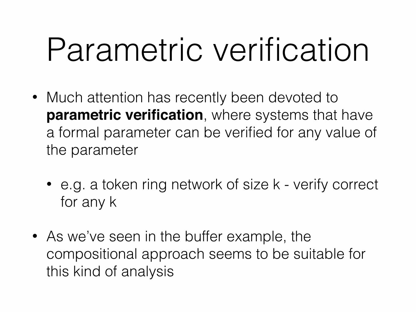
Parametric verification• Much attention has recently been devoted to

parametric verification, where systems that have a formal parameter can be verified for any value of the parameter

• e.g. a token ring network of size k - verify correct for any k

• As we’ve seen in the buffer example, the compositional approach seems to be suitable for this kind of analysis

Partial order reduction• Improving the current tools for PNBs

• Is working with LTS/automata really a good idea?

• concurrency is ignored…

• Can we combine compositionality with efficient techniques such as unfolding?

• Use SMT-solvers for performance?

BibliographyP. Sobocinski, Representations of Petri net interactions, CONCUR `10

R. Bruni, H. Melgratti, U. Montanari, A connector algebra for P/T nets interactions, CONCUR `11

R. Bruni, H. Melgratti, U. Montanari, P. Sobocinski, Connector Algebras for C/E and P/T Nets' Interactions, Log. Meth. Comput. Sci., 2013

P. Sobocinski, Nets, relations and linking diagrams, CALCO `13

P. Sobocinski and O. Stephens, A programming language for spatial distribution of net systems, Petri Nets `14

J. Rathke, P. Sobocinski and O. Stephens, Compositional reachability in Petri nets, Reachability Problems `14

F. Bonchi, P. Sobocinski and F. Zanasi, A Categorical Semantics of Signal Flow Graphs, CONCUR `14

F. Bonchi, P. Sobocinski and F. Zanasi, Full abstraction for Signal Flow Graphs, PoPL`15

Documents

Compositional model checking of concurrent systems, with