Embed Size (px)
Citation preview
COMPLEX ANALYSISFall 2006
Christer Bennewitz
Månne ifrån högre zoneranalytiska funktionersvaret nu dig finna låtapå odödlighetens gåta?
F. Läffler

Copyright c© 2006 by Christer Bennewitz
Preface
These notes are basically a printed version of my lectures in complexanalysis at the University of Lund. As such they present a limited viewof any of the subject matters brought up, caused by the time constraintsone is faced by in a series of lectures. The core of the subject, presentedin Chapter 3, is very strongly influenced by the treatment in Ahlfors’Complex Analysis, one of the genuine masterpieces of the subject. Anyreader who wants to find out more is advised to read this book.
Mathematical prerequisites are in principle the mathematics coursesgiven in the first two semesters in Lund. Most importantly, this in-cludes a reasonably complete discussion of analysis in one and severalvariables and basic facts about series of functions including absoluteand uniform convergence. A course in topology is also useful, but notessential. Primarily, a familiarity with the concept of a connected setis of use.
Egevang, August 2006
Christer Bennewitz
i

Contents
Preface i
Chapter 1. Complex functions 11.1. The complex number system 11.2. Polar form of complex numbers 41.3. Square roots 51.4. Stereographic projection 71.5. Möbius transforms 101.6. Polynomials, rational functions and power series 16
Chapter 2. Analytic functions 232.1. Conformal mappings and analyticity 232.2. Analyticity of power series; elementary functions 272.3. Conformal mappings by elementary functions 33
Chapter 3. Integration 373.1. Complex integration 373.2. Goursat’s theorem 403.3. Local properties of analytic functions 453.4. A general form of Cauchy’s integral theorem 483.5. Analyticity on the Riemann sphere 51
Chapter 4. Singularities 534.1. Singular points 534.2. Laurent expansions and the residue theorem 564.3. Residue calculus 594.4. The argument principle 65
Chapter 5. Harmonic functions 735.1. Fundamental properties 735.2. Dirichlet’s problem 79
Chapter 6. Entire functions 856.1. Sequences of analytic functions 856.2. Infinite products 876.3. Canonical products 906.4. Partial fractions 946.5. Hadamard’s theorem 96
Chapter 7. The Riemann mapping theorem 101iii
iv CONTENTS
Chapter 8. The Gamma function 105
CHAPTER 1
Complex functions
1.1. The complex number system
Recall that a group (G, ∗) is a set G provided with a binary opera-tion1 ∗ satisfying the following properties:
(1) For all elements x, y and z ∈ G holds (x ∗ y) ∗ z = x ∗ (y ∗ z).(associative law)
(2) There exists a neutral element e ∈ G with the properties x∗e =e ∗ x = x for every x ∈ G.
(3) Every element x ∈ G has an inverse x−1 with the propertiesx ∗ x−1 = x−1 ∗ x = e.
Exercise 1.1. Show that a set provided with an associative binaryoperation can have at most one neutral element.Hint: Show that if the set has a ‘left neutral’ element and a ‘rightneutral’ element, they must coincide.
Exercise 1.2. Show that if a set has an associative binary opera-tion with neutral element, then any element of the set has at most oneinverse.Hint: Show that if an element has a ‘left inverse’ and a ‘right inverse’,then these must coincide.
A group may also have the property(4) For all elements x and y ∈ G holds x∗y = y∗x. (commutative
law)in which case the group is called commutative or Abelian (after NielsHenrik Abel (1802–1829)). Familiar examples of Abelian groups are(Z, +), the integers under ordinary addition; (R, +), the real num-bers under addition; (Rn, +), the set of n-tuples of real numbers under(vector) addition; and (R \ 0, ·), the non-zero real numbers undermultiplication. As an example of a non-Abelian group, consider theset of all rotations around lines through the origin in 3-dimensionalspace; the binary operation is the ordinary composition of maps. Thereader should check these examples carefully; in particular, find theneutral elements and inverses in these groups.
1That is, a map ∗ : G × G → G, so that for every pair of elements x, y of G,there is a unique element of G denoted by x ∗ y.
1
2 1. COMPLEX FUNCTIONS
A field (F, +, ·) is a set F provided with two binary operations +and ·, such that (F, +) is an Abelian group and, if 0 denotes the neutralelement of this group, also (F \0, ·) is an Abelian group. In additionthe distributive laws
(x + y) · z = x · z + y · z,x · (y + z) = x · y + x · z.
hold for all elements x, y and z ∈ F . It is usual to denote the neutralelement of (F \ 0, ·) by 1.
Exercise 1.3. Prove that in any field F holds 0 · x = x · 0 = 0for all x ∈ F (as always, 0 denotes the neutral element of the group(F, +)).
Exercise 1.4. Prove that a field does not have any non-zero divi-sors of zero, i.e., if xy = 0, then either x = 0 or y = 0.
Familiar examples of fields are (Q, +, ·), the rational numbers underordinary addition and multiplication, and (R, +, ·). We shall show, inthis section, that there is precisely one reasonable way of making theEuclidean plane into a field. By introducing Cartesian coordinatesthis plane may be identified with the Abelian group (R2, +), and wewill make this into a field by extending the usual multiplication of anelement of R2 by a real number. The resulting field is the field C ofcomplex numbers.
To see how to make the definition, assume we have already managedto construct our field C. Then there is a multiplicative neutral element,which we will for the moment denote by 1, to distinguish it from thereal number 1. We may identify R with the set of real multiples of 1(explain!) and may therefore consider R as a subset of C. Let e bean element of R2 which is linearly independent of 1, so that 1, e is abasis in R2. Any element z ∈ C may then be written z = x1 + yewith real numbers x and y. In particular, there are real numbers aand b such that e2 = a1 + be so that z2 = (x2 + ay2)1 + (2xy + by2)e(note that 1 · 1 = 1, e · 1 = e). Now clearly z2 is real if y = 0 (sinceactually z itself is, by the identification above). But z2 will also be realif x = − b
2y. We then get z2 = (a+ b2
4)y2. We can not have a+ b2
4≥ 0 by
Exercise 1.4 since then (z− y√
a + b2
4)(z + y
√a + b2
4) = 0, but neither
of the factors is 0 unless their e-component y = 0. Hence a + b2
4< 0.
If we set y = 1/√−(a + b2
4) we therefore get z2 = −1.
Roughly, we have seen that if we can define a multiplication inR2 which makes it into a field with addition being the ordinary vectoraddition, then there exists an element the square of which is −1 (rather,the additive inverse of the multiplicative neutral element). We pick onesuch element (we will see later that there are precisely two), denote it
1.1. THE COMPLEX NUMBER SYSTEM 3
by i and call it the imaginary unit. If we use 1, i as a basis we maytherefore write any element in the plane as x1 + yi with real x, y. Forconvenience we will actually write it x + iy from now on.
It is important to note that we have not yet shown that it is possibleto make a field of the plane; we have just seen that if it is possible,then we may identify the x-axis with the real numbers and the y-axiswith the multiples of an element, the square of which is −1.
Exercise 1.5. Show that if we calculate with symbols x+iy, wherex and y are real numbers, according to the usual rules for adding andmultiplying numbers and in addition use i2 = −1, then all the require-ments for a field are satisfied.
From now on the field we have constructed is denoted by C andcalled the field of complex numbers. Note that the field of real numbersis an ordered field. This means that we have a relation < defined amongthe real numbers such that
(1) If x and y ∈ R, then exactly one of x < y, y < x and x = y istrue.
(2) Sums and products of positive (i.e., > 0) numbers are positive.We have not introduced anything similar for the complex numbers forthe simple reason that it can not be done.
Exercise 1.6. Show that in an ordered field squares of non-zeroelements are always > 0. Use this to show that if it were possible tomake C into an ordered field, then both 1 > 0 and −1 > 0, and hencealso 0 > 0, a contradiction.
As a final note to this first section, the fact that the Euclidean planecan be made into a field is extremely useful in all areas of mathematicsand its applications. Since we live in a 3-dimensional (at least) world, itwould, from the point of view of applications, be very useful if we couldmake 3-dimensional space into a field as well. In the early part of thenineteenth century, this is exactly what the famous Irish mathematicianW. R. Hamilton tried, unsuccessfully, to do.
Exercise 1.7. Try to show that Hamilton was doomed to fail. Tosimplify things, you may require that the complex plane should bea 2-dimensional restriction of the 3-dimensional field. Show that theexistence of divisors of zero can not be avoided.
Hamilton succeeded (1843) to introduce a multiplication in R4 whichmakes this into a field, with the minor defect that the multiplicativegroup is not Abelian (such a structure is called a skew field). Hamiltoncalled his structure the quaternions ; this structure actually stronglyhints that it would be profitable, in physics, to consider the world 4-dimensional, with time as the fourth dimension.
4 1. COMPLEX FUNCTIONS
Exercise 1.8. Consider the set of symbols x+ iy + ju+ kv, wherex, y, u and v are real numbers, and the symbols i, j, k satisfy i2 =j2 = k2 = −1, ij = −ji = k, jk = −kj = i and ki = −ik = j. Showthat using these relations and calculating with the same formal rulesas in dealing with real numbers, we obtain a skew field; this is the setof quaternions.
1.2. Polar form of complex numbers
In the complex number z = x + iy the real number x is called thereal part of z, x = Re z, and the number y is called the imaginarypart of z, y = Im z. There is of course nothing imaginary whateverabout the imaginary part; the reasons for this curious appellation arehistoric. If we introduce the notation z for the complex number x− iy,called the complex conjugate of z, we see that Re z = 1
2(z + z) and
Im z = 12i
(z − z). In particular, z is real (i.e., has imaginary part 0)precisely if z = z. If z has real part 0, so that z = −z, one calls zpurely imaginary. We define the absolute value |z| of z = x + iy to be|z| =
√x2 + y2. This is of course the ordinary length of z, considered
as a vector in the plane, provided we draw 1, i as orthonormal vectors.A very useful observation is that zz = |z|2.
Exercise 1.9. Show this and that for any complex numbers z andw we have
(1) z + w = z + w,(2) zw = z · w,(3) |zw| = |z||w|.
It is worth remarking how one carries out division by a complexnumber. Since the complex numbers constitute a field, every non-zerocomplex number has a multiplicative inverse, i.e., we can divide by it;namely, if z 6= 0 and w are complex numbers, then there is a uniquecomplex number u, denoted w
z, such that zu = w. The question is,
how does one write the quotient on the standard form as real part plusi times imaginary part. To see how, multiply through by z to obtain|z|2u = zw. Since |z|2 6= 0 we can divide by this (real) number, and sou = zw/|z|2. So, to write w/z on standard form, multiply numeratorand denominator by z.
Exercise 1.10. Write 1+2i3+4i
on standard form.
The geometric interpretation of addition is already familiar, sincethis is the ordinary vector addition in the plane. To get a geometricpicture of multiplication, we introduce polar coordinates in the plane inthe following way. If z 6= 0, then z/|z| is located somewhere on the unitcircle; hence we can find an angle θ such that z/|z| = cos θ+ i sin θ. Wemay therefore write z on polar form as z = |z|(cos θ + i sin θ) where θis called the argument of z and is denoted θ = arg z. It is unfortunate,
1.3. SQUARE ROOTS 5
but extremely important that arg z is NOT uniquely determined byz; adding any integer multiple of 2π to θ gives another, equally valid,value for arg z. When one therefore speaks of ‘the’ argument for acomplex number, one means one of the infinitely many possible valuesof the argument. Another, less serious ambiguity, is that we have notassigned an argument to the number 0; it is usual to allow any realnumber whatsoever as a valid argument for 0.
Now suppose z = |z|(cos θ + i sin θ) and w = |w|(cos φ + i sin φ)are complex numbers. Then zw = |z||w|(cos θ cos φ − sin θ sin φ +i(cos θ sin φ + sin θ cos φ)) = |zw|(cos(θ + φ) + i sin(θ + φ)) accordingto the addition formulas for sin and cos. Thus, when calculating theproduct of two complex numbers the absolute values are multiplied andthe arguments are added. In particular, multiplication by a complexnumber of absolute value 1 is equivalent to a rotation with an angleequal to the argument of the given number.
Exercise 1.11. Write the number z =√
3 + i on polar form andthen calculate z13 on standard form.
1.3. Square roots
Working with real numbers it is possible to find the square rootof any non-negative number; to obtain a unique number the squareroot is required to be non-negative as well. After introducing complexnumbers we can, for any given real number, find a real or complexnumber whose square is the given number. Of course, not much wouldbe gained unless we could actually find the square root of any complexnumber as well. This means that we would like to be able to find asolution to z2 = w for any complex number w. Suppose w = u + ivand let z = x + iy (in situations like this it is always assumed that u,v, x and y are real numbers). Since z2 = x2 − y2 + 2ixy we need tosolve the nonlinear system
(1.1)
x2 − y2 = u,
2xy = v.
in two real unknowns x and y. Squaring and adding the two equationswe get, after extracting a (real) square root, that x2 + y2 =
√u2 + v2
(this simply expresses the fact that |z|2 = |w|, which has to be true inview of Exercise 2.1). Together with the first equation this shows that
(1.2)
x = ±√
12(√
u2 + v2 + u),
y = ±√
12(√
u2 + v2 − u).
Note that all the expressions within square roots are non-negative nomatter what u and v are, so these are ordinary real square roots. (1.2)therefore give all possible solutions of (1.1), and it is easily verified that
6 1. COMPLEX FUNCTIONS
the first equation is actually satisfied, whereas the second is satisfiedif and only if one chooses the right combination of signs, so that thereare actually always precisely two distinct complex numbers z satisfyingz2 = w, unless w = 0 in which case z = 0 is the only solution. Sincea quadratic equation can be solved by extracting square roots one noweasily sees that any quadratic equation with complex coefficients alwayshas a complex root. In fact, if counted by multiplicity there are alwaysexactly two roots (we will return later to the concept of multiplicityfor a root).
We have seen that we can always extract square roots of a complexnumber w, and that there are always (unless w = 0) exactly two suchnumbers. The question arises: Which of the two possibilities are weto denote by the symbol
√w? Since the complex numbers are not
ordered there is no simple answer to this question, as in the real case.To analyze the situation we write w = |w|(cos θ+ i sin θ) on polar form.If z2 = w, then clearly |z| =
√|w|, and if φ is an argument for z, then
2φ must be an argument for w. The simplest choice for φ is thereforeto set φ = θ/2. Which number z we get this way obviously dependson the choice of θ, which is only determined up to an integer multipleof 2π. If we add 2π to θ we will add π to φ, which will replace z by−z. Adding or subtracting further multiples of 2π to θ will not yieldany more values for z, so we have again seen that there are exactlytwo square roots of any non-zero number. We can write any complexnumber w on polar form with an argument θ in the interval −π < θ ≤ πand choosing the argument of the square root to be φ = θ/2 we willget −π
2< φ ≤ π
2.
This is one way of assigning a unique value to the square root ofany complex number. Considering z as a function of w this is calledthe principal branch of the square root; if w is a non-negative realnumber it obviously coincides with the usual real square root. Thevalues of the principal branch of the square root are all in the righthalf plane, i.e., they have non-negative real part. There are, however,other ways of choosing a branch of the square root that are sometimesmore convenient. On may for example restrict θ to the interval 0 ≤θ < 2π, which will give the argument of the square root in the interval0 ≤ φ < π, i.e., this branch of the root has all its values in the upperhalf plane.
Why can one not, once and for all like in the case of the real squareroot, choose a particular branch and stick to it? The reason is problemswith continuity. Suppose we have a nice curve in the w-plane whichintersects the negative real axis. If we take the square root of this, usingthe principal branch, the image of the curve in the z-plane will jumpfrom a point on the negative imaginary axis to a point on the positiveimaginary axis; we have lost the continuity of the curve. Another choiceof branch might solve the problem for a particular curve, but it is clear
1.4. STEREOGRAPHIC PROJECTION 7
that no choice of branch will be suitable for all curves. Since there isno choice of branch which will work best in all situations one must notuse the notation
√without specifying which branch of the square root
one is talking about.The need to deal with several different branches occurs for all kinds
of other complex functions and is a major complicating factor in thetheory. There is a sophisticated and completely satisfactory solutionto the problem, namely the introduction of the concept of a Riemannsurface. Unfortunately we can not go into that here.
1.4. Stereographic projection
Since we have a notion of distance (i.e., d(z, w) = |z −w|) in C wemay view C as a metric space. It is clear that this space is completein the sense that any Cauchy sequence converges; to see this note thatsince |Re z| ≤ |z| and | Im z| ≤ |z| ≤ |Re z| + | Im z| for any z ∈ Cit follows that if zj = xj + iyj, j = 1, 2, . . . is a Cauchy sequence inC, then xj, j = 1, 2, . . . and yj, j = 1, 2, . . . are Cauchy sequences inR. Furthermore, if xj → x ∈ R and yj → y ∈ R as j → ∞, thenxj + iyj → x + iy ∈ C as j →∞. Thus the completeness of C followsfrom that of R.
From the point of view of topology, it would be even better if Cwere compact, i.e., any open cover of C should have a finite subcover.This is not true, however, as can be seen by considering the open coverof C consisting of all open balls |z| < R centered at 0, which obviouslyhas no finite subcover. One can make C compact without changingits topology by adding (at least) one ‘ideal’ point and modifying themetric. This one-point compactification of the complex plane is veryimportant in the theory of functions of a complex variable and we willgive a very enlightening geometric interpretation of it in this section.
Imagine C as the x1x2-plane in R3 and let S2 be the unit sphere;it will intersect C along the unit circle. Call the point (0, 0, 1) on thesphere the North pole N (so that (0, 0,−1) is the South pole). We canmap C in a one-to-one fashion onto S2 \ N by mapping z ∈ C ontothe point (x1, x2, x3) ∈ S2 such that the straight line connecting z withN goes through (x1, x2, x3). This map is called stereographic projectionand has many interesting properties, as we shall see. In this connectionS2 is called the Riemann sphere.
It is nearly obvious that this stereographic projection is a bi-con-tinuous map, using the topology induced by the metric of R3. To makeabsolutely sure, let us find the mapping explicitly. The line throughN and z = x + iy ∈ C is (x1, x2, x3) = (0, 0, 1) + t(x, y,−1). Theintersection with S2 is given by t satisfying t2(x2 + y2) + (1 − t)2 = 1which gives t = 0, i.e., N , and the more interesting t = 2/(x2 +y2 +1).
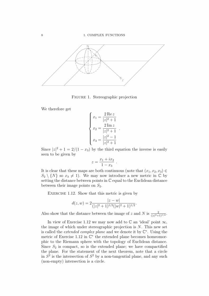
8 1. COMPLEX FUNCTIONS
Figure 1. Stereographic projection
We therefore get
x1 =2 Re z
|z|2 + 1
x2 =2 Im z
|z|2 + 1
x3 =|z|2 − 1
|z|2 + 1
.
Since |z|2 + 1 = 2/(1 − x3) by the third equation the inverse is easilyseen to be given by
z =x1 + ix2
1− x3
.
It is clear that these maps are both continuous (note that (x1, x2, x3) ∈S2 \ N so x3 6= 1). We may now introduce a new metric in C bysetting the distance between points in C equal to the Euclidean distancebetween their image points on S2.
Exercise 1.12. Show that this metric is given by
d(z, w) = 2|z − w|
(|z|2 + 1)1/2(|w|2 + 1)1/2.
Also show that the distance between the image of z and N is 2(|z|2+1)1/2 .
In view of Exercise 1.12 we may now add to C an ‘ideal’ point ∞,the image of which under stereographic projection is N . This new setis called the extended complex plane and we denote it by C∗. Using themetric of Exercise 1.12 in C∗ the extended plane becomes homeomor-phic to the Riemann sphere with the topology of Euclidean distance.Since S2 is compact, so is the extended plane; we have compactifiedthe plane. For the statement of the next theorem, note that a circlein S2 is the intersection of S2 by a non-tangential plane, and any such(non-empty) intersection is a circle.
1.4. STEREOGRAPHIC PROJECTION 9
Theorem 1.13. The image of a straight line in C under stereo-graphic projection is a circle through N , with N excluded. The imageof a circle in C under stereographic projection is a circle not containingN . The inverse image of any circle on S2 is a straight line togetherwith ∞ if the circle passes through N , otherwise a circle.
Proof. Since a straight line in the x1x2-plane together with Ndetermines a unique plane, the intersection of which with S2 is theimage of the straight line we only need to consider the case of a circlein C. If it has center a and radius r its equation is |z − a|2 = r2 or|z|2−2 Re(az)+ |a|2 = r2. Substituting z = x1+ix2
1−x3into this, using that
x21 + x2
2 + x23 = 1 and x3 6= 1, we get 1 + x3 − 2x1 Re a − 2x2 Im a +
(1 − x3)(|a|2 − r2) = 0 which is the equation of a plane. Conversely,a circle on the Riemann sphere is determined by three distinct points.The inverse images of these three points determine a circle in C. Theimage of this circle is clearly the original circle. ¤
In view of this theorem we will by a circle in the extended planemean either a line together with ∞, or an actual circle.
A map is called conformal if it preserves angles and their orientation(we will give a more exact definition in Chapter 2.1). A surface is givenan orientation by assigning to each point a normal direction whichvaries continuously with the point. For example, the usual orientationof C is given by letting at each point the normal point upwards, i.e., inour present picture in the direction of the x3-axis. Similarly, we maygive the Riemann sphere an orientation by letting the normal pointtowards the origin.
The angle between two smooth curves in an oriented surface at apoint of intersection of the curves is the angle between the tangentsat the point. There are two such angles, the sum of which is π. Ifthe curves are given in a certain order, the positively oriented anglebetween them is that angle through which one has to turn the firsttangent vector so as to coincide with the second tangent vector, turn-ing counterclockwise as seen from the normal to the surface. A strictdefinition would of course have to be freed from such obviously intuitivegeometric concepts, but we will not attempt this here.
Theorem 1.14. Stereographic projection is conformal.
Proof. Consider two curves intersecting at z and their tangentsat z in C. Together with N the tangents determine two planes thatintersect the Riemann sphere in two circles through N . The tangentsto the circles at N are in these planes and also in the plane through Nparallel to C. It follows that they are parallel to the original tangentvectors so that viewed from inside the sphere they give rise to an angleequal to but of opposite orientation to the original angle.
10 1. COMPLEX FUNCTIONS
The circles intersect also at the image of z on the sphere, and aretangent to the images of the curves there. The angles at the two pointswhere the circles intersect are equal but of opposite orientation bysymmetry (the two angles are images of each other under reflection inthe plane through the origin and parallel to the normals of the planesof the circles). The theorem now follows. ¤
Although the proof above is very geometric in nature it is actu-ally not difficult to make it analytic, using the fact that stereographicprojection is a differentiable map, but we will not do that here.
1.5. Möbius transforms
A Möbius transform (also called a linear fractional transformation)
is a non-constant mapping of the form z 7→ f(z) =az + b
cz + dfor complex
numbers a, b, c and d. To begin with we consider this defined in Cexcept, if c 6= 0, for z = −d/c. The fact that the mapping is non-constant means that (a, b) is not proportional to (c, d). This can beexpressed by requiring ad− bc 6= 0 which is always assumed from nowon. Clearly we get the same mapping if we multiply all the coefficientsa, b, c, d by the same non-zero number so that although the mappingis determined by the matrix ( a b
c d ) any non-zero multiple of this matrixgives the same mapping. The requirement ad − bc 6= 0 means thatthe determinant is 6= 0 so multiplying by an appropriate number wemay always assume that the determinant is 1. This determines thecoefficients up to a change in sign of all of them.
It is clear that if c = 0, then f(z) → ∞ as z → ∞. On the otherhand, if c 6= 0, then f(z) →∞ as z → −d/c and f(z) → a/c as z →∞.We may therefore extend the definition of f to all of the extended planeC∗ in such a way that the extended function is a continuous functionof C∗ into C∗. We will always consider Möbius transforms as definedin the extended plane, or equivalently on the Riemann sphere, in thisway. We have the following interesting proposition.
Proposition 1.15. If f and g are Möbius transforms correspond-ing to the matrices A and B, then the composed map f g is a Möbiustransform corresponding to the matrix AB.
Exercise 1.16. Prove Proposition 1.15.
Since the set of all non-singular 2 × 2 matrices is a group undermatrix multiplication, it follows that so are the Möbius transforms.This means that any Möbius transform has an inverse which is also aMöbius transform.
Exercise 1.17. Find all Möbius transforms T for which T 2 = T .
1.5. MÖBIUS TRANSFORMS 11
Among other things this means that a Möbius transform is a home-omorphism of the extended plane onto itself, i.e., a continuous one-to-one and onto map whose inverse is also continuous. But Möbiustransforms have more surprising properties. Recall that we by a circlein the extended plane mean either an actual circle in the plane or astraight line together with ∞.
Theorem 1.18. Möbius transforms are conformal and circle-pre-serving, i.e., any circle in the extended plane is mapped onto a circlein the extended plane.
Proof. The theorem is obvious for certain simple special cases,namely a translation z 7→ z + b, a rotation z 7→ az where |a| = 1and a dilation z 7→ az where a > 0. It is therefore also true for amultiplication z 7→ az where 0 6= a ∈ C, since this is the compositeof the rotation z 7→ a
|a|z and the dilation z 7→ |a|z. Composing amultiplication with a translation the theorem follows for a linear mapz 7→ az + b where a 6= 0, and hence for any Möbius transform for whichc = 0. If c 6= 0 we have az+b
cz+d= bc−ad
c1
cz+d+ a
cso that this map is the
composite of three maps, the first and last being linear and the middlemap is the inversion z 7→ 1/z. The theorem therefore follows if we canprove it for an inversion.
If the image of z under stereographic projection is (x1, x2, x3), thenwe have z = x1+ix2
1−x3so that 1/z = 1−x3
x1+ix2= (1 − x3)
x1−ix2
x21+x2
2. Since
(x1, x2, x3) is on the unit sphere we have x21 + x2
2 = 1 − x23 so that
1/z = x1−ix2
1+x3. Therefore 1/z is the inverse stereographic projection of
(x1,−x2,−x3). The map that takes (x1, x2, x3) into this is a rotationaround the x1-axis by an angle π. This is obviously a circle-preservingand conformal map, and since we know that also stereographic projec-tion is circle-preserving and conformal it follows that the inversion hasthe desired properties. The proof is now complete. ¤
Exercise 1.19. Prove the theorem by calculation, not using stere-ographic projection.
Note that since removing a circle from the extended plane leavesa set with exactly two components, and since Möbius transforms arecontinuous in the extended plane, the interior of any circle in the planeis mapped either onto the interior or onto the exterior, including ∞,of another circle. This follows from the fact that continuous mapspreserve connectedness.
Exercise 1.20. Prove the statement above in detail.
Sets that are left invariant under a mapping are obviously importantcharacteristics of the map. For a Möbius transform one may for exam-ple ask which circles it leaves invariant, or conversely, which Möbiustransforms leave a given circle invariant. We will consider some such
12 1. COMPLEX FUNCTIONS
problems later. Right now we will instead ask for fixpoints of a giventransform, i.e., points left invariant by the map. By our definition ofthe image of ∞, this is a fixpoint if and only if the map is linear. Alinear map z 7→ az + b also has the finite fixpoint z = b/(1− a), exceptif a = 1. Thus, a translation which is not the identity has only thefixpoint ∞, but any other linear map which is not the identity hasexactly one finite fixpoint as well. For a Möbius transform z 7→ az+b
cz+d
with c 6= 0 the equation for a fixpoint becomes z(cz+d) = az+b whichis a quadratic equation. It therefore has either two distinct roots or adouble root. We have therefore proved the following proposition.
Proposition 1.21. A Möbius transform different from the identityhas either one or two fixpoints, as a map defined on the extended plane.
Exercise 1.22. Find the fixed points of the linear transformations
w =z
2z − 1, w =
2z
3z − 1, w =
3z − 4
z − 1, w =
z
2− z.
In particular, a Möbius transform that leaves three distinct pointsinvariant is the identity. It also follows that there can be at mostone Möbius transform that takes three given, distinct points into threespecified, distinct points. Because, if there were two, say f and g, thenf−1g would be a transform different from the identity and leaving thegiven points invariant. Conversely, we will prove that there actuallyalways exists a Möbius transform that takes the given points into thespecified ones. To see this, define the cross ratio of four distinct pointsz0, z1, z2, z3 in C∗ by
(z0, z1, z2, z3) =z0 − z2
z0 − z3
/z1 − z2
z1 − z3
when all the points are finite. If one of them is ∞, the cross ratio isdefined as the appropriate limit of the expression above. The followingproposition follows by inspection.
Proposition 1.23. Suppose z1, z2, z3 are distinct points in C∗. Theunique Möbius transform taking these points to 1, 0,∞ in order is z 7→(z, z1, z2, z3).
It is now clear that to find the unique Möbius transform taking thedistinct points z1, z2, z3 into the distinct points w1, w2, w3 in order, onesimply has to solve for w in (w,w1, w2, w3) = (z, z1, z2, z3).
Exercise 1.24. Find the Möbius transformation that carries 0, i,−i in order into 1, −1, 0.
Exercise 1.25. Show that any Möbius transformation which leavesR ∪ ∞ invariant may be written with real coefficients.
Exercise 1.26. Show that the map z 7→ z−1z+1
maps the right half-plane (i.e., the set Re z > 0) onto the interior of the unit circle.
1.5. MÖBIUS TRANSFORMS 13
Two points z and z∗ are said to be symmetric with respect to R ifz∗ = z. If T is a Möbius transform that maps R∪∞ onto itself, thenaccording to Exercise 1.25 one may write T with real coefficients. Itfollows that Tz and T (z∗) are symmetric with respect to the real axisif and only if z and z∗ are. To generalize the concept of symmetry withrespect to the real axis to symmetry with respect to any circle in theextended plane we make the following definition.
Definition 1.27. Let Γ be a circle in C∗. Two points z and z∗ aresaid to be symmetric with respect to Γ if there is a Möbius transformT which maps Γ onto the real axis for which T (z∗) = Tz.
By the reasoning just before the definition it is clear that this is agenuine extension of the notion of conjugate points and that z and z∗
are symmetric with respect to Γ precisely if T (z∗) = Tz for any Möbiustransform T that takes Γ to the real axis. For, if T and S both take Γonto the real axis and T (z∗) = Tz, then U = ST−1 maps the real axisonto itself so that S(z∗) = UT (z∗) = U(Tz) = UTz = Sz. There istherefore for every z precisely one point z∗ so that z, z∗ are symmetricwith respect to Γ. A similar calculation proves the next theorem.
Theorem 1.28. Suppose S is a Möbius transform that takes thecircle Γ ∈ C∗ onto the circle Γ′ ∈ C∗. Then the points z and z∗ aresymmetric with respect to Γ if and only Sz and S(z∗) are symmetricwith respect to Γ′.
Proof. If T maps Γ onto the real axis, then U = TS−1 mapsΓ′ onto the real axis. But US(z∗) = T (z∗) and USz = Tz so thatUS(z∗) = USz if and only if T (z∗) = Tz. The theorem follows. ¤
In short, Theorem 1.28 says that symmetry is preserved by Möbiustransforms. The next theorem allows us to calculate the symmetricpoint to any given z and circle.
Theorem 1.29. If Γ is a straight line, then z and z∗ are symmetricwith respect to Γ precisely if they are each others mirror image in Γ.If Γ is a genuine circle with center a and radius R, then a and ∞ aresymmetric with respect to Γ. If z is finite and 6= a, then z and z∗ aresymmetric precisely if (z∗ − a)(z − a) = R2.
Proof. If Γ is a straight line it is mapped onto the real axis by atranslation or a rotation and these transformations obviously preservemirror images.
If Γ is a circle with center a and radius R the map z 7→ i z−a−Rz−a+R
takesΓ onto the real axis (since a + R 7→ 0, a − R 7→ ∞ and a − iR 7→ 1).Now a and ∞ are mapped onto −i and i respectively, so they are asymmetric pair. If z has neither of these values a simple calculationshows that z and z∗ are mapped onto conjugate points precisely if(z∗ − a)(z − a) = R2. ¤
14 1. COMPLEX FUNCTIONS
In particular the fact that the center of a circle and∞ are symmetricwith respect to the circle are often very helpful in trying to find mapsthat take a given circle into another.
Exercise 1.30. Find the Möbius transform which carries the circle|z| = 2 into |z + 1| = 1, the point −2 into the origin, and the origininto i.
Exercise 1.31. Find all Möbius transforms that leave the circle|z| = R invariant. Which of these leave the interior of the circleinvariant?
Exercise 1.32. Suppose a Möbius transform maps a pair of con-centric circles onto a pair of concentric circles. Is the ratio of the radiiinvariant under the map?
Exercise 1.33. Find all circles that are orthogonal to |z| = 1 and|z − 1| = 4.
We will end this section by discussing conjugacy classes of Möbiustransforms.
Definition 1.34. Two Möbius transforms S and T are called con-jugate if there is a Möbius transform U such that S = U−1TU .
Conjugacy is obviously an equivalence relation, i.e., if we writeS ∼ T when S is conjugate to T , then we have:
(1) S ∼ S for any Möbius transform S. (reflexive)(2) If S ∼ T , then T ∼ S (symmetric)(3) If S ∼ T and T ∼ W , then S ∼ W . (transitive)
It follows that the set of all Möbius transforms is split into equivalenceclasses such that every transform belongs to exactly one equivalenceclass and is equivalent to all the transforms in the same class, but tono others.
Exercise 1.35. Prove the three properties above and the statementabout equivalence classes. What are the elements of the equivalenceclass that contains the identity transform?
The concept of conjugacy has importance in the theory of (discrete)dynamical systems. This is the study of sequences generated by theiterates of some map, i.e., if S is a map of some set M into itself,one studies sequences of the form z, Sz, S2z, . . . where z ∈ M . Thissequence is called the (forward) orbit of z under the map S. Oneis particularly interested in what happens ‘in the long run’, e.g., forwhich z’s the sequence has a limit (and what the limit then is), forwhich z’s the sequence is periodic and for which z’s there seems to beno discernible pattern at all (‘chaos’). Note that if S = U−1TU , thenSn = U−1T nU so that all maps in the same conjugacy class behavequalitatively in the same way, at least with respect to the properties
1.5. MÖBIUS TRANSFORMS 15
listed above. It therefore seems natural to try to find, in each conjugacyclass, some particularly simple map for which the questions above areparticularly simple to answer. In other words, one looks for a ‘canonicalrepresentative’ in each equivalence class. We will carry out this for thecase of Möbius transforms.
If S = U−1TU and z is a fixpoint of S, then Uz is a fixpoint of Tsince TUz = USz = Uz. If S has only one fixpoint z0 we may chooseV so that V z0 = ∞. Then V SV −1 has only the fixpoint ∞ and istherefore a translation z 7→ z + b for some b 6= 0. If we set U = 1
bV it
follows that USU−1z = z + 1. If S has two fixpoints z1 and z2 we maychoose U so that Uz1 = 0 and Uz2 = ∞. Then T = USU−1 has thefixpoint ∞, so it is linear, Tz = az + b, and it also has the fixpoint 0,so b = 0. Now set, for λ 6= 0,
Tλz =
z + 1 for λ = 1 ,
λz for 0 6= λ 6= 1 .
We have then proved most of the following theorem.
Theorem 1.36. For every Möbius transform S different from theidentity there exists λ 6= 0 such that S ∼ Tλ. If Tλ ∼ Tµ, then eitherλ = µ or λ = 1/µ.
Proof. It only remains to prove the last statement. But this isclear if λ = 1, since this is the only value for which Tλ has just onefixpoint. We may therefore assume that λ and µ are both 6= 1 (and ofcourse non-zero). But if UTλ = TµU and Uz = az+b
cz+dwe obtain
(1.3)aλz + b
cλz + d= µ
az + b
cz + d
for all z. Since ad− bc 6= 0 we can not have d = c = 0. If d 6= 0, settingz = 0 gives b/d = µb/d so that b = 0 and therefore a 6= 0. If now c 6= 0,setting z = −d/c we get ∞ on the right but not the left. It followsthat c = 0 and (5.2) becomes λ = µ. On the other hand, if d = 0 wemust have c 6= 0 and so z = ∞ gives a/c = µa/c. It follows that a = 0.In this case (5.2) becomes λ = 1/µ and the proof is complete. ¤
What we have proved is that each conjugacy class different fromthe class of the identity contains one of the operators Tλ and alsoT1/λ, but no other operators of this form. We may therefore with anyMöbius transform S associate the corresponding unique (non-ordered)pair (λ, 1/λ) of reciprocal complex numbers, called the multiplier of S.The multiplier is thus a conjugacy invariant. Note that some Tλ leavethe interior of certain circles in the extended plane invariant. Namely,T1 leaves all halfplanes above or below a horizontal line invariant. Ifλ > 0 (but 6= 1), then Tλ leaves all halfplanes bounded by a line throughthe origin invariant. Finally, if |λ| = 1 but λ 6= 1, then Tλ leaves theinteriors and exteriors of any circle concentric with the origin invariant.
16 1. COMPLEX FUNCTIONS
On the other hand, if λ is neither positive nor of absolute value 1there is no disk which is invariant under Tλ. Show this as an exercise!The transforms in the conjugacy class of T1 are called parabolic, those inthe conjugacy class of Tλ for some λ > 0 but 6= 1 are called hyperbolicand those in the conjugacy class of Tλ for some λ 6= 1 with |λ| = 1are called elliptic. The reason for these names will be clear from theresult of Exercise 1.37. The remaining Möbius transforms are calledloxodromic. This is because they are conjugate to a Tλ for which thesequence of iterates z, Tλz, T
2λz, . . . lie on a logarithmic spiral, which
under stereographic projection becomes a curve known as a loxodrome.
Exercise 1.37. Suppose that the coefficients of the transformation
Sz =az + b
cz + d
are normalized by ad−bc = 1. Show that S is elliptic if 0 ≤ (a+d)2 < 4,parabolic if (a + d)2 = 4, hyperbolic if (a + d)2 > 4 and loxodromic inall other cases. Hint: The determinant and the trace a + d of a matrix( a b
c d ) is invariant under conjugation by an invertible matrix.
Exercise 1.38. Show that a linear transformation which satisfiesSn = S for some integer n is necessarily elliptic.
Exercise 1.39. If S is hyperbolic or loxodromic, show that Snzconverges to a fixpoint as n →∞, the same for all z which are not equalto the other fixpoint. The exceptional fixpoint is called repelling, theother one attractive. What happens when n → −∞? What happensin the parabolic and elliptic cases?
Exercise 1.40. Find all linear transformations that are rotationsof the Riemann sphere.Hint: The antipodal point to a point on the unit sphere is obtained bymultiplication by −1. Use the fact that an antipodal pair is mappedonto an antipodal pair by a rotation.
1.6. Polynomials, rational functions and power series
We define a polynomial to be a complex-valued function p of acomplex variable given by a formula p(z) = anz
n + an−1zn−1 + · · · +
a1z + a0 where the coefficients a0, . . . an are complex numbers, an 6= 0,and n is a non-negative integer, called the degree of the polynomial,deg p. The function identically equal 0 is also a polynomial, of degree−∞. The sum of two polynomials of degrees n and m is a polynomialof degree ≤ max(n,m). The product of two polynomials of degrees nand m is a polynomial of degree n + m. The division algorithm saysthat if p and q are polynomials, then there are unique polynomials kand r with deg r < deg q such that p = kq + r. From this follows thefactor theorem which states that if p(a) = 0, then z− a divides p. The
1.6. POLYNOMIALS, RATIONAL FUNCTIONS AND POWER SERIES 17
proof is simply the observation that since p(z) = k(z)(z− a) + r wherer is constant (of degree < 1), then r = 0 if and only if p(a) = 0. Itis of course possible that the quotient k is also divisible by z − a. If jis the largest integer such that (z − a)j divides p, then j is called themultiplicity of a as a zero of p.
It also follows from the factor theorem that two polynomials p, qfor which p(z) = q(z) for all z ∈ C have to be identical, i.e., have thesame coefficients.
A very important fact about polynomials (which is only true if weconsider polynomials in the complex domain) is the fundamental the-orem of algebra which says that any non-constant polynomial has azero. We will prove this later, but assume it for the present. Com-bining the fundamental theorem of algebra with the factor theorem iteasily follows that if we add up the multiplicities of all the zeros of apolynomial p (‘count the zeros with their multiplicities’), the sum willbe the degree of p.
Also for complex functions the concepts of limit and continuityare of central importance. However, since complex numbers are justvectors in R2 , where we in addition has defined a multiplication, wecan take these concepts over from the calculus of several real variables.For reference we nevertheless state the definitions
Definition 1.41. Suppose f is a complex-valued function of eithera real or complex variable, with domain Ω ⊂ R or Ω ⊂ C.
• If a is a point in the closure of Ω, we say that limz→a f(z) = Aif A is a complex number such that for every ε > 0 there is aδ > 0 with the property that |f(z) − A| < ε whenever z ∈ Ωand 0 < |z − a| < δ.
• If a ∈ Ω we say that f is continuous at a if limz→a f(z) = f(a).All the standard calculation rules for limits and continuity familiar
from calculus continue to hold in this context, with exactly the sameproofs, so we will not dwell on this. We also remind the reader of theconcept of uniform convergence for a sequence of functions.
Definition 1.42. Suppose f and f1, f2, . . . are complex-valuedfunction of either a real or complex variable, with domain Ω ⊂ Ror Ω ⊂ C. If K ⊂ Ω we say that fj → f uniformly on K if for everyε > 0 there is a real number N such that |fj(z) − f(z)| < ε for allz ∈ K if j ≥ N .
As a function in C a polynomial is continuous; this follows easilysince constant polynomials and the polynomial z obviously are contin-uous, and any other polynomial can be built up from these by mul-tiplications and additions so the continuity follows from the standardcalculation rules for limits.
A rational function is a quotient r(z) = p(z)/q(z) where p and q arepolynomials and q not identically 0 (if q is constant r is a polynomial).
18 1. COMPLEX FUNCTIONS
It follows that r is continuous as a function in C in all points whichare not zeros of q. We may assume that p and q have no common non-constant polynomial factors (the common divisor to two polynomialsof largest degree can always be found by a purely algebraic device, theEuclidean algorithm). Hence p and q have no common zeros. It followsthat r(z) →∞ as z tends to any zero of q. As z →∞ we have r(z) → 0if deg p < deg q and r(z) → ∞ if deg p > deg q. If deg p = deg q, thenr(z) → a/b where a and b are the highest order coefficients of p and qrespectively.
A power series is a series
(1.4)∞∑
n=0
an(z − a)n
where a, a0, a1, a2, . . . are given complex numbers and z a complex vari-able. In many respects such series behave like ‘polynomials of infiniteorder’ and that is actually how they were viewed until the end of the19:th century. The very first question to ask is of course: For whichvalues of z does the series converge? In order to answer this questionwe make the following definition.
Definition 1.43. Let the radius of convergence for (1.4) be
R = supr ≥ 0 | a0, a1r, a2r2, . . . is a bounded sequence .
Then R is either a number ≥ 0 or R = ∞.
The explanation for the definition is in the following theorem.
Theorem 1.44. For |z − a| > R the series (1.4) diverges and for|z − a| < R it converges absolutely. The convergence is uniform onevery compact subset of |z − a| < R.
In order to prove the theorem we need a few results which shouldbe well known in the context of functions of a real variable.
Theorem 1.45. An absolutely convergent complex series is conver-gent.
Proof. For any complex number z we have |Re z| ≤ |z| and| Im z| ≤ |z| ≤ |Re z| + | Im z|. Hence, if
∑ |an| is convergent, thenby comparison the real series
∑Re an and
∑Im an are absolutely con-
vergent, to x and y say. The theorem now follows from
|N∑
n=0
an − x− iy| ≤ |N∑
n=0
Re an − x|+ |N∑
n=0
Im an − y| → 0 as N →∞ .
¤The next theorem is the complex version of what is usually known
under the silly name of Weierstrass’ M-test.
1.6. POLYNOMIALS, RATIONAL FUNCTIONS AND POWER SERIES 19
Theorem 1.46. Let A be a subset of C and f1, f2, . . . a sequence ofcomplex functions defined on A and such that |fn(z)| ≤ an for all z ∈ Aand n = 1, 2, . . . . If
∑∞n=0 an converges, then
∑∞n=0 fn(z) converges
uniformly in A.
Proof. By Theorem 1.45 the series∑
fn(z) converges absolutelyfor every z ∈ A; call the sum s(z). Then
|s(z)−N∑
n=0
fn(z)| = |∞∑
n=N+1
fn(z)| ≤∞∑
n=N+1
|fn(z)| ≤∞∑
n=N+1
an .
The last member does not depend on z and tends to 0 as N →∞. Thetheorem follows. ¤
Proof of Theorem 1.44. If |z − a| > R then an(z − a)n, n =0, 1, 2, . . . is an unbounded sequence and hence can not converge to 0.Hence the power series diverges.
If r < R, then there exists ρ > r such that anρn, n = 0, 1, 2, . . . is
a bounded sequence; let C be a bound. Then if |z − a| ≤ r we have|an(z − a)n| ≤ |an|rn = |anρn|(r/ρ)n ≤ C(r/ρ)n. Since a geometricseries with quotient 0 ≤ r/ρ < 1 is convergent, the theorem followsfrom Theorem 1.46 (any compact subset of |z − a| < R is a subset of|z − a| ≤ r for some r < R). ¤
Here is the complex version of another well known theorem.
Theorem 1.47. Suppose f1, f2, . . . is a sequence of continuous,complex functions converging uniformly to f on the set M . Then fis continuous on M .
The proof is word for word the same as in the case of real func-tions so we will not repeat it here. We have the following corollary ofTheorems 1.44 and 1.47.
Corollary 1.48. If R is the radius of convergence of (1.4), then(1.4) is a continuous function of z for |z − a| < R.
Proof. The partial sums of a power series are polynomials andtherefore continuous. Since any z in the disk |z − a| < R is an in-terior point of a compact subset of the disk the claim follows fromTheorems 1.44 and 1.47. ¤
So far we have said nothing about convergence on the boundary ofthe circle of convergence. There is a good reason for this; nothing muchcan be said in general. One can have divergence at every point of thecircle, convergence at some points and divergence at others or one canhave absolute convergence at every point of the circle. A general resultby Carleson (1966) says that if
∑∞n=0 |anR
n|2 converges, then (1.4) willconverge ‘almost everywhere’ on the circle, in the sense of Lebesgueintegration. On the other hand, there are examples (the first one given
20 1. COMPLEX FUNCTIONS
by Kolmogorov in 1926) for which anRn → 0 such that (1.4) diverges
for every point on the circle.
Exercise 1.49. Show that∑∞
n=0 zn diverges at every point of itscircle of convergence, that
∑∞n=0 zn/n converges for some but not all
points on its circle of convergence and that∑∞
n=0 zn/n2 converges ab-solutely for all points on its circle of convergence.
It is often possible to find the radius of convergence for a givenpower series by inspection and use of the definition. As an aid in caseswhere this might be difficult we have the following two theorems.
Theorem 1.50. limn→∞
|an|1/n = 1/R. This is to be interpreted byusing the conventions 1/0 = ∞ and 1/∞ = 0.
Here we have defined limn→∞
cn = lim supn→∞ cn = limn→∞ supk≥n ck
for a real sequence c0, c1, . . . .
Proof. Let L = limn→∞
|an|1/n. If r < 1/L, then |an|1/n < 1/r for allsufficiently large n. Hence |anrn| < 1 for such n, so the sequence anr
n,n = 0, 1, 2, . . . is bounded. Hence 1/L ≤ R.
If r > 1/L, then there exists ρ, r > ρ > 1/L, so that |an|1/n >1/ρ for infinitely many n. Hence |anr
n| = |anρn|(r/ρ)n > (r/ρ)n for
infinitely many n. Since (r/ρ)n →∞ the sequence anrn, n = 0, 1, 2, . . .can not be bounded and so 1/L ≥ R and the proof is complete (checkthe cases L = 0 and L = ∞ separately). ¤
Theorem 1.51. If limn→∞ |an/an+1| exists it is equal to R.
Proof. Let L = limn→∞ |an/an+1|. If r < L, then r < |an/an+1|for all sufficiently large n. It follows that |an+1r
n+1| < |anrn| for such
n so that anrn, n = 0, 1, 2, . . . , being of eventually decreasing absolute
value, is bounded. Hence L ≤ R.On the other hand, if r > L, choose ρ so that r > ρ > L. Then
there exists N such that ρ > |an/an+1| for n ≥ N . It follows forsuch n that |an+1ρ
n+1| > |anρn| > · · · > |aNρN |. We therefore have|anrn| = |anρ
n|(r/ρ)n > |aNρN |(r/ρ)n →∞ as n →∞ (we may assumeaN 6= 0 since this must be true eventually for limn→∞ |an/an+1| toexist). It follows that L ≥ R so the theorem is proved. ¤
1.6. POLYNOMIALS, RATIONAL FUNCTIONS AND POWER SERIES 21
Exercise 1.52. Find the radius of convergence for the followingpower series:
(a)∞∑
n=0
n2z2 (b)∞∑
n=0
nnzn
(c)∞∑
n=0
zn
(n!)2(d)
∞∑n=0
2−nzn
(e)∞∑
n=2
zn
ln n(f)
∞∑n=1
2n
n2zn
(g)∞∑
n=1
zn
arctan n(h)
∞∑n=0
(n2 + 2n)zn
(i)∞∑
n=0
cos(nπ/4)zn (j)∞∑
n=1
2n + 2−n
nzn
(k)∞∑
n=1
n1/nzn (l)∞∑
n=0
(2n + (−2)n + 1)zn
(m)∞∑
n=0
(√
n2 + 1−√
n2 − 1)zn (n)∞∑
n=0
(n + 2)3
32n+1zn
(o)∞∑
n=0
21/n
2nzn (p)
∞∑n=1
2n
√n
z2n
(q)∞∑
n=1
zn
1 + 2 + · · ·+ n(r)
∞∑n=1
(1 + 12
+ · · ·+ 1n)zn
(s)∞∑
n=0
zn2
(t)∞∑
n=1
zn2
n2
(u)∞∑
n=1
zn2
n(v)
∞∑n=0
z4n
2n + n2
(w)∞∑
n=0
(sin n)zn (x)∞∑
n=1
nn
n!zn
(y)∞∑
n=1
(arctan 1n)zn (z)
∞∑n=0
(a
n
)zn
(å)∞∑
n=1
(2n
n
)zn (ä)
∞∑n=0
(3n + 1)!
(n!)4zn
(ö)∞∑
n=0
2√
nzn (ööh)∞∑
n=1
(1 + 1n)n2
zn

CHAPTER 2
Analytic functions
2.1. Conformal mappings and analyticity
Definition 2.1. A map f : Ω → C, where Ω is an open subset ofC, is called conformal if it satisfies the following conditions:
(1) As a map from a subset of R2 into R2, f is differentiable.(2) f preserves angles of intersection between smooth curves.(3) f preserves orientation in the sense that the determinant of
the total derivative of the map is > 0.
To explain the definition in more detail, note that if z = x + iy,where x and y are real, then f(z) = u(x, y)+ iv(x, y) where u and v arereal-valued functions of two real variables, so the action of f can also bedescribed by the mapping ( x
y ) 7→(
u(x,y)v(x,y)
). The first condition of the
definition then says that this map should be differentiable. Recall thatthis implies that the partial derivatives ux, uy, vx and vy exist and thatthe chain rule can be applied when composing with other differentiablemaps. Also recall that the existence of the partials is not enough toguarantee differentiability, but if the partials are continuous, then themap is differentiable.
We measure the angle between two non-zero vectors α and β ∈ Rn
by the expression 〈α,β〉‖α‖‖β‖ , where 〈·, ·〉 is the usual scalar product and
‖ · ‖ the Euclidean norm (the actual angle is arccos of this). If t 7→γ(t) = γ1(t) + iγ2(t) is a differentiable curve in Ω, then its tangentvector is γ′ or, expressed as a column vector,
(γ′1γ′2
). The image f γ of
γ under f is another differentiable curve. According to the chain ruleits tangent vector is J
(γ′1γ′2
)where J = ( ux uy
vx vy ) is the Jacobi matrix ortotal derivative of the map. The second point of the definition thenmeans that the linear map given by the Jacobi matrix maps any twovectors onto two vectors which make the same angle as the originalvectors. The third point simply means that the Jacobian | ux uy
vx vy | =uxvy − uyvx ≥ 0 in Ω.
Exercise 2.2. Show that the map z 7→ z satisfies the two firstpoints of Definition 2.1, but reverses the orientation (i.e., the Jaco-bian is < 0). Such a map is called anti-conformal. Show that anyanti-conformal map is of the form z 7→ f(z) where f is conformal.
23
24 2. ANALYTIC FUNCTIONS
This shows that there is really no need to study anti-conformal mapsseparately from conformal maps.
We have the following basic theorem.Theorem 2.3. Suppose f = u + iv is conformal in Ω. Then the
partials of u and v satisfy the Cauchy-Riemann equations
(2.1)
ux = vy,
uy = −vx.
Conversely, if ( uv ) satisfy the Cauchy-Riemann equations, the corre-
sponding map is differentiable and its Jacobi matrix does not vanish atany point in Ω, then the map is conformal.
The slight asymmetry in the statement of Theorem 2.3 will be re-moved later; in fact, we will later show (see the discussion after Corol-lary 4.23) that the Jacobi matrix can not vanish in any domain wherethe map is conformal.
Proof. Suppose f is conformal and let α and β be the columnvectors in the Jacobi matrix. Since multiplication by the Jacobi matrixpreserves angles the vectors ( 1
0 ) and ( 01 ) are mapped onto orthogonal
vectors, i.e., α and β are orthogonal. Similarly, the vectors ( 11 ) and
( 1−1 ) are mapped onto orthogonal vectors. Since the scalar product of
α+β and α−β is ‖α‖2−‖β‖2 it follows that α and β also have the samelength, so that ( ux
vx ) = ± ( vy
−uy
). The Jacobian is therefore ±(u2
x + u2y).
To preserve orientation we must choose the plus sign. It follows thatany conformal map satisfies the Cauchy-Riemann equations.
Conversely, if the map satisfies the Cauchy-Riemann equations, isdifferentiable, and has non-vanishing Jacobi matrix, then this matrixis
√u2
x + u2y O where O is an orthogonal matrix with determinant one,
i.e., a rotation. The map is therefore conformal. ¤Exercise 2.4. Show that the map z 7→ z2 is conformal in any open
set not containing the origin.We will now connect the geometric notion of a conformal map with
the analytic notion of complex derivative. We first need a definition.Definition 2.5. A complex-valued function f defined in an open
subset of C is said to be differentiable at a if
limz→a
f(z)− f(a)
z − a
exists. The limit is called the derivative of f at a and is denoted byf ′(a).
All the elementary properties of derivatives that we know from thetheory of a real function of one variable continue to hold, with essen-tially the same proofs. We collect some such properties in the nexttheorem.
2.1. CONFORMAL MAPPINGS AND ANALYTICITY 25
Theorem 2.6. Suppose that f is differentiable at a. Then(1) f is continuous at a.(2) Cf is differentiable at a with derivative Cf ′(a) for any con-
stant C.(3) If g is differentiable at a, then so is f +g, fg and, if g(a) 6= 0,
f/g and
(f + g)′(a) = f ′(a) + g′(a)
(fg)′(a) = f ′(a)g(a) + f(a)g′(a)
(f/g)′(a) = (f ′(a)g(a)− f(a)g′(a))/g(a)2
(4) If g is differentiable at f(a), then g f is differentiable at aand the chain rule (g f)′(a) = g′(f(a))f ′(a) is valid.
(5) If f ′(a) 6= 0 and the inverse f−1 is defined in a neighborhoodof f(a) and is continuous at b = f(a), then the inverse isdifferentiable at b and (f−1)′(b)) = 1/f ′(a).
(6) Polynomials and rational functions are differentiable wherethey are defined (as functions in C) and their derivatives arecalculated in the same way as in the case of real polynomialsand rational functions.
Exercise 2.7. Prove Theorem 2.6.
Exercise 2.8. Show that any branch of√
z is differentiable forz 6= 0 and calculate the derivative.
We will later prove (see Corollary 4.23) that if f is differentiablein a neighborhood of a, then the assumption f ′(a) 6= 0 implies all theother assumptions of Theorem 2.6 (5). We are now ready to state thesecond main result of this section.
Theorem 2.9. f = u + iv has a complex derivative at z = a + ib
if and only the map ( xy ) 7→
(u(x,y)v(x,y)
)is differentiable and the Cauchy-
Riemann equations (2.1) are satisfied at (a, b). We also have f ′(z) =ux(x, y) + ivx(x, y) = v′y(x, y)− iu′y(x, y).
Proof. For f to be differentiable with derivative a+ib at z = x+iymeans that
|f(z + w)− f(z)− (a + ib)w| = |w|r(w) where r(w) → 0 as w → 0 .
Similarly, for ( uv ) to be differentiable at (x, y) with a Jacobi matrix(
a b−b a
)satisfying the Cauchy-Riemann equations means that
∥∥∥∥(
u(x + h, y + k)− u(x, y)v(x + h, y + k)− v(x, y)
)−
(a b−b a
)(hk
)∥∥∥∥ = ‖(h, k)‖‖ρ(h, k)‖
where ρ(h, k) → 0 as (h, k) → 0. But if f = u + iv and w = h + ikthe left hand sides of these two relations are equal so the theoremfollows. ¤
26 2. ANALYTIC FUNCTIONS
If g is a complex-valued function of a real variable with real andimaginary parts u and v respectively, we say that g is differentiable if uand v are, and define g′ = u′+iv′. Using the equivalence in Theorem 2.9it then follows from the chain rule for vector-valued functions of severalvariables that if g is a complex-valued, differentiable function of onevariable with range in the domain of a complex differentiable functionf , then the chain rule d
dtf(g(t)) = f ′(g(t))g′(t) is valid.
There are some alternative ways of expressing the Cauchy-Riemannequations which are sometimes used. If we view f as a function ofx = Re z and y = Im z it is clear that the Cauchy-Riemann equationsare equivalent to f ′x + if ′y = 0. Note also that this means that if thecomplex derivative f ′ exists, then f ′ = f ′x = −if ′y.
The differential of f as a function of (x, y) is df = f ′xdx + f ′ydy, inparticular dz = dx + idy and dz = dx − idy. We can therefore writedf = 1
2(f ′x−if ′y)dz+ 1
2(f ′x+if ′y)dz and for this reason one introduces the
notation ∂f∂z
= 12(f ′x− if ′y) and
∂f∂z
= 12(f ′x + if ′y). The Cauchy-Riemann
equations may then be expressed as ∂f∂z
= 0, and then ∂f∂z
= f ′.We also have df = ∂f
∂zdz+ ∂f
∂zdz, so if we introduce the holomorphic
differential ∂ by ∂f = ∂f∂z
dz and the anti-holomorphic differential ∂
by ∂f = ∂f∂z
dz we have d = ∂ + ∂, and the Cauchy-Riemann equationsmay also be written as ∂f = 0. An analytic function is therefore asolution of the homogeneous ∂ equation (pronounced d-bar equation).This also means that f is analytic if df = ∂f = ∂f
∂zdz = f ′(z) dz.
Definition 2.10. A function f : M → C where M ⊂ C is calledanalytic in M if it is defined and differentiable in some open set con-taining M .
Note that to say that f is analytic in a means more than just havinga derivative in a; f has to be differentiable in a whole neighborhood ofa. A function which is analytic in an open set Ω is often said to beholomorphic in Ω, and the set of functions which are holomorphic in Ωis often denoted H(Ω).
Practically always the only domains of analyticity that are of inter-est are connected. There are two notions of connectivity in common use,arcwise connectivity which is used in calculus, and the more generalnotion of connectivity from topology. Since we are always consideringopen domains, it makes no difference whether you use one or the other,since they are equivalent for open sets. For convenience, we will usethe word region to denote an open, connected subset of the complexplane (or, occasionally, of the Riemann sphere).
We end by a simple result that we will use in the next section.
Theorem 2.11. Suppose f is analytic in a region Ω and that f ′(z) =0 for all z ∈ Ω. Then f is constant in Ω.
2.2. ANALYTICITY OF POWER SERIES; ELEMENTARY FUNCTIONS 27
We will actually prove much stronger results later; in fact it will beenough to assume that the zeros of f ′ has a point of accumulation inΩ for the conclusion to be valid.
Proof. If z ∈ Ω and w ∈ C is sufficiently close to z, then the linesegment between z and w is entirely in Ω. For 0 ≤ t ≤ 1 we then obtainddt
f(z + t(w− z)) = f ′(z + t(w− z))(w− z) = 0 using the remark afterthe proof of Theorem 2.9. Thus Re f and Im f are constant on the linesegment. In particular, f(z) = f(w) so that f is locally constant. Nowpick a ∈ Ω and let A = z ∈ Ω | f(z) = f(a). Then A is open bywhat we just saw. But also Ω \ A is open for the same reason. Sincea ∈ A we have A 6= ∅. Since Ω is connected we therefore must haveΩ \ A = ∅, i.e., A = Ω. In other words, f is constant. ¤
2.2. Analyticity of power series; elementary functions
We will first continue the study of power series begun in Chap-ter 1.6. First of all, if a power series really behaves ‘like a polynomialof infinite order’, then we should be able to differentiate the series likea finite sum, i.e., term by term, and actually obtain the derivative ofthe sum of the series.
In order to prove this, we first note that the usual derivative andintegral of a function of one variable extends to the case of a complex-valued function of a real variable in an obvious manner. If f is sucha function, with real and imaginary parts u and v, we simply definef ′(t) = u′(t) + iv′(t) and
∫ b
af(t) dt =
∫ b
au(t) dt + i
∫ b
av(t) dt. This
means that we define f as differentiable respectively integrable if itsreal and imaginary parts have these properties.
It immediately follows that the fundamental theorem of calculusddt
∫ t
af = f(t) holds also for complex-valued, continuous functions f .
It is also more or less obvious that the usual calculation rules for deriva-tives and integrals continue to hold. In particular, the integral is inter-val additive and linear, so that
b∫
a
f =
c∫
a
f +
b∫
c
f
b∫
a
(αf + βg) = α
b∫
a
f + β
b∫
a
g
for a < c < b and arbitrary constants α and β if f and g are bothintegrable on [a, b]. We also have the triangle inequality
(2.2)∣∣∣
b∫
a
f(t) dt∣∣∣ ≤
b∫
a
|f(t)| dt.
28 2. ANALYTIC FUNCTIONS
This is less obvious, but follows from
Re(eiθ
b∫
a
f)
=
b∫
a
Re(eiθf) ≤b∫
a
|f |
by choosing θ = − arg(∫ b
af).
As already mentioned we also have the chain rule ddt
f(g(t)) =f ′(g(t))g′(t) if f is analytic and g is a differentiable complex-valuedfunction of a real variable. Thus, if f is analytic in a region containingthe line segment connecting z and z +h, then d
dtf(z + th) = hf ′(z + th)
so that 1h(f(z + h)− f(z)) =
∫ 1
0f ′(z + th) dt if the derivative is contin-
uous. An immediately consequence is the following lemma.
Lemma 2.12. Suppose f is analytic with continuous derivative ina compact set K containing the line segment connecting z and z + hwhere h 6= 0. Then we have | 1
h(f(z + h)− f(z)| ≤ supK |f ′|.
Proof. By the triangle inequality we obtain
∣∣∣f(z + h)− f(z)
h
∣∣∣ =∣∣∣
1∫
0
f ′(z + th) dt∣∣∣ ≤
1∫
0
|f ′(z + th)| dt ≤ supK|f ′|.
¤Exercise 2.13. Prove the theorem without assuming f ′ to be con-
tinuous.Hint: Use the mean value theorem on Re(eiθf(z + th)).
We can now state our theorem about differentiating power series.
Theorem 2.14. If the series f(z) =∑∞
k=0 ak(z − a)k has conver-gence radius R, then f has derivatives of all orders for |z − a| < R.The derivatives are calculated by term by term differentiation, andthe resulting series all have radius of convergence R. In particular,f ′(z) =
∑∞k=1 kak(z − a)k−1.
Proof. We will prove the statement for the first derivative. Thestatement for the higher derivatives then follows immediately. Clearly
g(z) =∞∑
k=1
kak(z − a)k−1
has the same radius of convergence as∑∞
k=1 kak(z − a)k and sincek√
k → 1 as k →∞, it follows from Theorem 1.50 that g has the sameradius of convergence as f .
If r < R the series∑∞
k=1 k|ak|rk−1 converges, and
1
h(f(z + h)− f(z)) =
∞∑
k=1
ak
h((z + h− a)k − (z − a)k).
2.2. ANALYTICITY OF POWER SERIES; ELEMENTARY FUNCTIONS 29
Now fix z, |z − a| < r. Then the terms of this series are continuousfunctions of h, with value kak(z − a)k−1 for h = 0. By Lemma 2.12the terms have absolute value less than k|ak|rk−1 if |z − a| < r and|z + h − a| ≤ r, so according to Theorems 1.46 and 1.47 the sum isa continuous function of h in |z + h − a| ≤ r. For h 6= 0 its valueis 1
h(f(z + h) − f(z)) and for h = 0 the value is g(z). Thus f is
differentiable and f ′(z) = g(z) for any z satisfying |z − a| < R. ¤
We will use Theorem 2.14 to introduce some more elementary func-tions. It is clear that the series
∑∞k=0
zk
k!converges for all z so that the
following definition is meaningful.
Definition 2.15. For any z ∈ C, let(1) ez =
∑∞k=0
zk
k!,
(2) sin z = eiz−e−iz
2i,
(3) cos z = eiz+e−iz
2.
These are all analytic functions in the whole plane. Such a functionis called entire. From the definition follows immediately that e0 = 1,sin 0 = 0 and cos 0 = 1. Furthermore, d
dzez = ez, d
dzcos z = − sin z
and ddz
sin z = cos z. It also follows that sin is odd (sin(−z) = − sin z)and cos even (cos(−z) = cos z) and that we have the power seriesexpansions sin z =
∑∞k=0
(−1)k
(2k+1)!z2k+1 and cos z =
∑∞k=0
(−1)k
(2k)!z2k.
Theorem 2.16. The functions of Definition 2.15 satisfy the follow-ing functional equations:
(1) ez+w = ezew, for any complex numbers z and w.(2) sin(z + w) = sin z cos w + cos z sin w,(3) cos(z + w) = cos z cos w − sin z sin w
for any complex numbers z and w.
Note that the particular case w = −z of (1) shows that e−zez = 1so that ez 6= 0 for all z ∈ C.
Proof. Given w ∈ C, let f(z) = e−zez+w. This is an entire func-tion with derivative f ′(z) = −e−zez+w + e−zez+w = 0 so it is constantby Theorem 2.11. Setting z = 0 we obtain e−zez+w = ew for all z andw. The special case w = 0 shows that e−zez = 1 so that e−z = 1/ez.The first formula now follows; the other formulas follow immediatelyfrom this by inserting the definitions of sin and cos in the formulas tothe right. ¤
Theorem 2.17. We have |ez| = eRe z. There exists a smallest realnumber π > 0 such that sin π = 0, and this number satisfies 2.8 < π <3.2. The exponential function has period 2πi, the functions sin and cosperiod 2π. All other periods are integer multiples of these.
30 2. ANALYTIC FUNCTIONS
Proof. First note that ex+iy = ex(cos y+ i sin y) by Theorem 2.16.Since the coefficients in the power series for ez are all real it followsthat as a function of a real variable, ex is real-valued. It is also > 0,since it is continuous, never = 0 and e0 = 1 > 0. Since it is also its ownderivative it follows that it is strictly increasing (and strictly convex).For similar reasons cos and sin are real-valued for real arguments andsince
(2.3) cos2 z + sin2 z = 1
(take w = −z in Theorem 2.16 (3)) it follows that cos y + i sin y is apoint on the unit circle for y ∈ R. Hence |ez| = eRe z.
We next note that if a real, continuous and non-constant functionis periodic, then all its periods are integer multiples of its smallestpositive period. First of all, since y is a period if and only if −y is,there are positive periods if there are any. Next, if there are arbitrarilysmall periods > 0, then given x and ε > 0 we can find a period a,0 < a < ε and an integer p such that |ap− x| < ε. Now f(0) = f(ap)and by continuity f(ap) → f(x) as ε → 0, so f is constant. Alsonote that the set of periods of f is closed, since if yj → y and all yj
are periods, then f(y + x) = lim f(yj + x) = f(x), so that also y is aperiod. If f is non-constant it therefore has a smallest positive perioda, and if b is another period, then for any integer q, b− aq is a period.But if q is the integer quotient and r the remainder when dividing bby a, then 0 ≤ r = b − aq < a. So, a can not be the smallest positiveperiod unless r = 0.
If now w is a period for the exponential function so that ez = ez+w
for all z, we see that this is equivalent to ew = 1. Taking absolute valuesit follows that Re w = 0. Setting w = iy we see that y is a real periodfor both sin and cos. Note that neither of these functions can havenon-real periods since we immediately obtain from Theorem 2.16 (2)respectively 2.16 (3) that w is a period of either of these functions ifand only if sin w = 0 and cos w = 1. By (2.3) the first of these relationsfollows from the second, which may be rewritten as (eiw−1)2 = 0. Thisis true if and only if iw is a period for ez. Therefore, sin and cos havethe same periods, they are real and y is the smallest positive periodof the trigonometric functions if and only if it is the smallest positivenumber for which cos y = 1.
Now cos y = 1 − 2 sin2 y2according to Theorem 2.16 (3) and (2.3).
It follows that y is the smallest positive number for which cos y = 1if and only if y
2is the smallest positive zero of sin. According to (2.3)
we must then have cos y2
= −1 and there can be no smaller positivenumbers for which cos takes the value −1. Now cos y
2= 2 cos2 y
4− 1 so
that y2has this property if and only if y
4is the smallest positive zero
for cos. It now only remains to show that cos actually has a smallestpositive zero, and to estimate its value.
2.2. ANALYTICITY OF POWER SERIES; ELEMENTARY FUNCTIONS 31
Since cos is continuous the set of its non-negative zeros is a closedset and therefore has a smallest element if it is non-empty. By (2.3)we have cos x ≤ 1 for real x and integrating this from 0 to x > 0 fourtimes we get in turn sin x ≤ x, 1 − cos x ≤ x2
2, x − sin x ≤ x3
6and
x2
2− 1 + cos x ≤ x4
24. It follows that for x > 0 we have 1− x2
2≤ cos x ≤
1 − x2
2+ x4
24(this may also be deduced from the fact that the power
series for cos is an alternating series). The first positive zeros of thetwo polynomials are
√2 > 1.4 and
√6− 2
√3 < 1.6 respectively. It
follows that cos has a smallest positive zero which is in the interval(1.4, 1.6). The proof is now complete. ¤
One may easily continue to define strictly all the usual (real) func-tions of elementary calculus and prove all the usual properties of them.We will assume this done; in particular x is the arclength of the arc ofthe unit circle beginning at 1 and ending at eix = cos x+ i sin x, so x isthe angle between the rays through these points starting at 0. We willalso use the common properties of the inverse tangent function.
If we want to extend the definition of the logarithm to the com-plex domain, we should find the inverse of the exponential function.However, since the exponential function is periodic it has no inverseunless we restrict its domain appropriately (cf. the definition of theinverse trigonometric functions). To see how to do this, let us attemptto calculate the inverse of the exponential function, i.e., to solve theequation z = ew for a given z.
We first note that we must assume z 6= 0, since the exponentialfunction never vanishes. Taking absolute values we find that |z| = eRe w
so that Re w = ln |z|, where ln is the usual natural logarithm of apositive real number. We also obtain z
|z| = ei Im w. Now cos 0 = 1 andcos π = −1 and since cos is continuous, it takes all values in [−1, 1] inthe interval [0, π]. Since Re z
|z| ∈ [−1, 1] we can find x ∈ [0, π] such thatcos x = Re z
|z| . It follows that sin x = ± Im z|z| . Changing the sign of x
changes the sign on sin x but leaves cos x unchanged. Therefore eithereix or e−ix equals z
|z| .We may therefore solve the equation for w given any z 6= 0. If w1
and w2 are two solutions, it follows that ew1−w2 = 1, so that w1 andw2 differ by an integer multiple of 2πi. We call any permissible valueof Im w an argument for z, and denote any such number by arg z.We should therefore define log z = ln |z| + i arg z. To get an actual(single-valued) function, we must make particular choices of arg z foreach z. We shall see later that in order to be able to this and obtaina continuous function, we can not allow all of C \ 0 in the domain.Intuitively it is clear that we must choose the domain such that thereare no closed curves in it that ‘go around’ the origin, since followingsuch a curve we would have changed the argument continuously by an
32 2. ANALYTIC FUNCTIONS
integer multiple of 2π when we arrive back at the starting point. Thisleads to the following concept.
Definition 2.18. A connected subset of the Riemann sphere iscalled simply connected if its complement is connected.
If Ω is a region where we want to define a single-valued, continuousargument function, it must not contain 0 or ∞, and to exclude thepossibility of having a closed curve in Ω that ‘winds around’ 0, weshould exclude from Ω a connected set containing both 0 and ∞. Nowsuppose we have selected a region Ω which is simply connected in C anddoes not contain 0, and one of the possible arguments for some pointin Ω. It seems plausible that this should determine a single-valued,continuous logarithm in Ω. We shall show later (see Theorem 3.19)that this is the case; we call such a function a branch of the logarithm.
The most important example is obtained when one chooses Ω tobe C with the non-positive part of the real axis removed, and fixesthe argument at 1 to be 0. This is called the principal branch of thelogarithm. The argument of any number in Ω is determined by therequirement that it is in (−π, π). The notation Log with a capital L issometimes used for this branch.
Another important case is when one instead removes the non-nega-tive real axis and fixes the argument at −1 to be π. The argumentis then in the interval (0, 2π). Other choices are obtained when oneremoves from C any smooth, non self-intersecting curve starting at0 and ending at ∞. In any case, it is not possible to talk about thecomplex logarithm without specifying which branch one is dealing with.
Theorem 2.19. Any branch of the logarithm is analytic with de-rivative 1/z.
Proof. For any z = x+ iy we have log(x+ iy) = u(x, y)+ iv(x, y)where u(x, y) = 1
2ln(x2 + y2) and v(x, y) = arctan y
x+ kπ, where k is
some integer except if x = 0 in which case v(x, y) = π2− arctan x
y+ kπ.
By continuity the same value of k has to be used in any sufficientlysmall neighborhood of z. Differentiating we therefore get ux(x, y) =
xx2+y2 , uy(x, y) = y
x2+y2 , vx(x, y) = − yx2+y2 and vy(x, y) = x
x2+y2 so thatthe Cauchy-Riemann equations are satisfied. Since the partials are allcontinuous for (x, y) 6= (0, 0), the function is analytic by Theorem 2.3.The derivative is ux + ivx = x−iy
x2+y2 = 1zso the proof is complete. ¤
Exercise 2.20. Prove Theorem 2.19 by use of Theorem 2.6 (5).
We are now able to define arbitrary powers of any complex numberw 6= 0. We set wz = ez log w, where log is some branch of the logarithm,giving rise to a branch of the power. By varying the branch, there istherefore in general infinitely many values of the power; e.g., ii = ei log i
and since log i = ln 1+ i arg i the possible values of log i are i(π2+2kπ),
2.3. CONFORMAL MAPPINGS BY ELEMENTARY FUNCTIONS 33
where k is an integer. Hence the possible values of ii are e−π2−2kπ.
There are therefore infinitely many possible values (note that they areall real!). In some cases the situation is simpler, however; if w is real> 0 one always uses the principal branch of the logarithm so that wz
for real z is the elementary exponential function with base w.One can of course also view the exponent as fixed and the base as
the variable; these are the power functions z 7→ zα. If α is an integerit is clear that the choice of branch for the logarithm is irrelevant; thefunction coincides with the elementary concept of a power function. Ifα is rational = n
mwhere m > 0 and n are integers with no common
factors, there are exactly m possible values of zα for each z 6= 0; oneusually says that there are m branches. This agrees with our discussionof the square root in Chapter 1.3. If α is irrational or non-real, how-ever, there are always infinitely many branches of the power. Differentpowers are said to be of the same branch if they are defined throughthe same branch of the logarithm.
Theorem 2.21. Any branch of zα is analytic (in its domain) withderivative αzα−1, using the same branch.
Proof. ddz
eα log z = αzeα log z = αe(α−1) log z. ¤
If α is real and > 0 the power function is also defined for z = 0,with value 0 and if α = 0 the power function is the constant 1.
2.3. Conformal mappings by elementary functions
We will here only give some examples of mappings induced by powerfunctions and by the exponential function and their combinations withMöbius transforms.
Suppose α ∈ R. That a branch of w = zα is defined in an open setΩ means that zα = eα log z for an appropriately chosen branch of thelogarithm. Note that those z ∈ Ω for which |z| = r are mapped onto|w| = rα so that circular arcs centered at the origin are mapped onto(other) circular arcs centered at the origin. Similarly, if z is on a rayarg z = θ we have arg w = αθ so rays from the origin are mapped ontoother rays from the origin. Also, angles at the origin are multipliedby a factor α so that the map is certainly not conformal there unlessα = 1. This is true even if α is an integer so that zα is well defined inthe whole plane. Note that the derivative vanishes at 0 then.
These observations show that a wedge domain, bounded by two raysfrom the origin making the angle φ may be mapped onto a half planeby applying a branch of zα where α = π/φ. More generally, any regionwith a corner at the origin may have this corner ‘straightened out’ byapplying an appropriate power function. Since any region bounded bytwo intersecting circular arcs may be mapped onto a wedge by a Möbiustransform taking the points of intersection to 0 and∞ respectively, any
34 2. ANALYTIC FUNCTIONS
such region may be mapped onto a half plane by composing a Möbiustransform and a power function.
Exercise 2.22. Construct a conformal mapping that takes the re-gion
|z + 3| <√
10,
|z − 2| <√
5,
onto the interior of the first quadrant.
Exercise 2.23. Map the region
0 < arg z < π/α , 0 < |z| < 1 ,
onto the interior of the unit circle (α ≥ 1/2).
Since ez = ex(cos y + i sin y) if z = x + iy it is clear that theexponential function takes any line parallel to the real axis into a rayfrom the origin. Similarly, any vertical line segment is taken into acircular arc centered at the origin and with angular opening equal tothe length of the line segment. This means that an infinite strip parallelto the real axis, i.e., a region of the type a < Im z < b, is mapped onto awedge domain by the exponential function. A half infinite strip definedby a < Im z < b, Re z < c is similarly mapped onto a circular sectorcentered at the origin.
Exercise 2.24. What is the image of the region 0 < Im z < 2πunder the map w = ez?
Exercise 2.25. Construct a conformal mapping of the region |z − 1| > 1,
|z| < 2,
onto the upper half plane.
Exercise 2.26. Construct a conformal map of the region−π/4 < arg z < π/4 ,
0 < |z| < R , (R > 1)
onto the interior of the unit circle, so that z = 1 is mapped onto theorigin. Calculate the length of the arc of the unit circle which is theimage of the arc −π/4 ≤ arg z ≤ π/4 ,
|z| = R .
Exercise 2.27. What is the image of the unit disk under the mapw = F (z) = (z + 1/z)/2, F (0) = ∞.Hint: Introduce W = w−1
w+1and Z = z−1
z+1.
2.3. CONFORMAL MAPPINGS BY ELEMENTARY FUNCTIONS 35
Exercise 2.28. Map the region a < arg z < b, where 0 < a <b < 2π, conformally onto the complex plane with the positive real axisremoved.
Exercise 2.29. Find a conformal map that takes
Ω =
|(1− i)z + (1 + i)z| < 2 ,
(1 + i)z + (1− i)z > 0 ,
onto
Ω′ = |z − 1− i| < 2 ,
−i(z − z) > 2 .
Exercise 2.30. Consider the conformal map given by cos z. Whatare the images of lines parallel to the real and imaginary axes? Whatis the image of the strip −π < Re z < π?

CHAPTER 3
Integration
3.1. Complex integration
Complex integration is at the core of the deeper facts about analyticfunctions. Here we will discuss the basic definitions.
Let γ be a piecewise differentiable curve in C. This means a complex-valued, continuous function defined on a compact real interval which iscontinuously differentiable except at a finite number of points, whereat least the left and right hand limits of the derivative exist. Thus itis described by an equation z = z(t) where a ≤ t ≤ b for some realnumbers a and b and z′ is continuous except for a finite number of jumpdiscontinuities. For convenience we will in the sequel call such a curvean arc.
If f is a continuous, complex-valued function of a complex variabledefined on an arc γ, then the composite function f(z(t)) is continuousand we make the following definition.
Definition 3.1.∫
γ
f(z) dz =
b∫
a
f(z(t))z′(t) dt.
If you know about line integrals and f = u+ iv, z = x+ iy you willrealize that
∫γf(z) dz is the line integral
∫
γ
u dx− v dy + i
∫
γ
v dx + u dy,
but we will not use this. It is, however, very important that thecomplex integral is independent of the parametrization of the arc γ.This means the following. A change of parameter is given by a piece-wise differentiable, increasing function t(s) mapping an interval [c, d]onto [a, b]. The usual change of variables formula then shows that∫
γf(z) dz =
∫ d
cf(z(t(s)))z′(t(s))t′(s) ds. Here z′(t(s))t′(s) is, by the
chain rule, the derivative of z(t(s)), so that the definition of the com-plex integral gives the same value whether we parametrize γ by z(t) orz(t(s)).
Note that the arc γ has an orientation, in that it begins at z(a) andends at z(b). If t(s) is a decreasing piecewise differentiable function,mapping [c, d] onto [a, b], then the equation z = z(t(s)) will give aparametrization of the opposite arc to γ, which we denote by −γ, in
37
38 3. INTEGRATION
that the initial point is now z(t(c)) = z(b) and the final point z(t(d)) =z(a). Thus we have
∫−γ
f(z) dz = − ∫γf(z) dz.
It is clear by the definition that the integral is linear in f , and alsothat if we divide an arc γ into two sub-arcs γ1 and γ2 by splittingthe parameter interval into two subintervals with no common interiorpoints (keeping the correct orientation), then
∫γf(z) dz =
∫γ1
f(z) dz+∫γ2
f(z) dz. It is now an obvious step to consider the sum of two (ormore) arcs γ1 and γ2 even if they are not sub-arcs of another arc, anddefine the integral over such a sum as the sum of the integrals over theindividual terms. Such a formal sum of arcs is called a chain. Given arcsγ1, . . . , γn we may integrate over chains of the form γ = a1γ1+· · ·+anγn,where the coefficients a1, . . . , an are arbitrary integers, indicating thatthe integral
∫γj
f enters in∫
γf with the coefficient aj. If aj = 0 the
arc γj can of course be left out of γ.Note that our notation for the opposite of an arc makes sense, in
that integrating over −γ amounts to integrating over (−1)γ. Very oftenwe will integrate over closed arcs. This means an arc where the initialand final points coincide. A simple arc is one without self-intersections;for a closed arc this means no self-intersections apart from the commoninitial and final point.
There is also a triangle inequality for complex integrals. From thedefinition of integral and the triangle inequality (2.2) it immediatelyfollows that ∣∣∣
∫
γ
f(z) dz∣∣∣ ≤
∫
γ
|f(z)| |dz|,
where the last integral is defined by∫
γ|f(z)| |dz| := ∫ b
a|f(z(t)||z′(t)| dt
and is called an integral with respect to arc-length. The reason forthis is, of course, that
∫γ|dz| =
∫ b
a|z′(t)| dt gives the length of the arc
γ. If you don’t know this already, you may take it as a definition oflength. Note that a very similar calculation to the one we did earliershows that an integral with respect to arc length is independent of theparametrization, and in this case also of the orientation of the arc.
Example 3.2. Suppose γ is the circle |z − a| = r, oriented byrunning through it counter-clockwise. A parametrization is z(t) =a + reit, 0 ≤ t ≤ 2π. We obtain z′(t) = ireit so that |z′(t)| = r. Thelength of the circle is therefore
∫ 2π
0rdt = 2πr, as expected.
It is possible to integrate along more general curves than thosethat are piece-wise differentiable, so called rectifiable curves. Thereis seldom any reason to do this in complex analysis, however. In fact,when integrating analytic functions the integral is, as we shall see later,independent of small changes in the path we integrate over, so it ispractically always enough to consider piece-wise differentiable arcs.
3.1. COMPLEX INTEGRATION 39
The elementary way of calculating integrals of a function of a realvariable is by finding a primitive of the integrand. This method canbe used also for complex integrals. Suppose that a continuous functionf has a primitive, i.e., a function F analytic on a continuously differ-entiable curve γ such that F ′ = f . Suppose z = z(t), a ≤ t ≤ b, is aparametrization of γ. Then
(3.1)∫
γ
f(z) dz =
b∫
a
f(z(t))z′(t) dt =
b∫
a
(F (z(t)))′ dt
=[F (z(t))
]b
a= F (z1)− F (z0),
where z0 = z(a) is the initial and z1 = z(b) the final point of γ. If γ isjust piece-wise continuously differentiable the same formula holds; oneonly has to use (3.1) on each differentiable piece and add the resultingformulas. The evaluations of the primitive at the intermediate pointswill then cancel, and we obtain (3.1) again.
So far the theory of analytic functions closely parallels the theoryof functions of a real variable. This is quite misleading, as we shallsee in the next section. The first indication that the theory of analyticfunctions is very different from one-variable real analysis comes whenone asks the question of which functions f of a complex variable have aprimitive. This turns out to require that f is analytic, but not even thisis enough. There are also requirements on the nature of the domain off , and these questions are a central theme for the theory of analyticfunctions. The starting point is the following theorem.
Theorem 3.3. Suppose f is continuous in a region Ω. Then f has
a primitive F in Ω if and only if∫
γ
f(z) dz = 0 for every closed arc
γ ⊂ Ω. It is enough if this is true for arcs made up solely of verticaland horizontal line segments.
Proof. If F is a primitive of f in Ω and γ a closed arc with initialand final points z1 = z0, then
∫γf(z) dz = F (z1) − F (z0) = 0 since
z1 = z0.Conversely, if the integral along closed arcs vanishes, pick a point
z0 ∈ Ω and define F (z) =∫
γf , where γ is an arc in Ω starting at z0
and ending at z. This gives an unambiguous definition of F , since if γis another such arc, then the arc γ − γ is a closed arc in Ω. Thus theintegral along γ has the same value as the integral along γ. We mayrestrict ourselves to arcs of the special type of the statement of thetheorem, since in an open, connected set Ω every pair of points may beconnected by an arc of this kind in Ω (show this as an exercise!).
It now remains to show that F is a primitive of f in Ω.
40 3. INTEGRATION
Writing z = x + iy with real x, y we shall calculate the partialderivatives of F with respect to x and y. To do this, let h ∈ R beso small that the line segment between z and z + h is contained in Ω.Then F (z +h)−F (z) =
∫ h
0f(z + t) dt. This is seen by choosing an arc
γ starting at z0 and ending at z to calculate F (z), and then calculatingF (z + h) by adding to γ the line segment connecting z to z + h, whichwe parametrize by z(t) = z + t, 0 ≤ t ≤ h.
By the fundamental theorem of calculus, differentiating with respectto h gives F ′
x(z) = f(z). Similarly, considering F (z + ih) − F (z) =
i∫ h
0f(z + it) dt we obtain F ′
y(z) = if(z). Thus the Cauchy-Riemannequation F ′
x + iF ′y = 0 is satisfied, and F ′ = F ′
x = f , so that F is aprimitive of f . ¤
3.2. Goursat’s theorem
In this section we shall begin to explore properties of analytic func-tions which show them to be very different in nature to differentiablefunctions of a real variable.
We first prove a fundamental theorem by Goursat (1905). We thenconsider integrals along the boundary of a rectangle. A rectangle is ofcourse a set defined by inequalities a ≤ Re z ≤ b, c ≤ Im z ≤ d, and theboundary consists of four line segments with endpoints at the pointsa+ ic, b+ ic, b+ id and a+ id. The boundary is therefore a closed arc,and we orient it by running through the vertices in the order described,ending up finally with a + ic again. This means we run through theboundary in the direction which has the interior of the rectangle tothe left of the boundary. This orientation of the boundary is calledpositive.
Theorem 3.4. Suppose f is analytic in a closed rectangle ( i.e., inan open set containing the rectangle) and let γ be the positively oriented
boundary of the rectangle. Then∫
γ
f(z) dz = 0.
Proof. Let R be the rectangle and I be the value of the integral.Now divide R into four congruent rectangles by one horizontal and onevertical cut, and let the integrals over the positively oriented boundariesof the sub-rectangles be Ij, j = 1, . . . , 4. A common side to two of therectangles will then be given opposite orientation in the correspondingintegrals. It follows that I = I1 + I2 + I3 + I4, since the contributionsfrom integrating over the cuts will cancel. Thus the absolute valueof at least one of the Ij will be ≥ |I|/4. Let R1 be a correspondingsub-rectangle and I1 the associated integral, so that |I| ≤ 4|I1|. Wecan now repeat the process with R1, and then repeat this process in-definitely. We obtain a nested1 sequence R1, R2, . . . of rectangles and
1i.e., each rectangle is contained in the previous one
3.2. GOURSAT’S THEOREM 41
a corresponding sequence I1, I2, . . . of integrals such that |I| ≤ 4n|In|for n = 1, 2, . . . .
The sequences of lower left corner real and imaginary parts in Rn
are both increasing, because the rectangles are nested, and boundedfrom above, because all rectangles are contained in R. It follows thatthe sequence of lower left corners converge to a point w ∈ R. Let d bethe diameter of R, i.e., the length of the diagonal. Then it is clear thatthe diameter of Rn is dn = 2−nd, so that given any neighborhood of w,Rn will be contained in this neighborhood for all sufficiently large n.
Now f is differentiable at w, so that |f(z)−f(w)z−w
− f ′(w)| < ε if zis sufficiently close to w. Denoting the expression inside the absolutevalue signs by ρ(z) we obtain f(z) = f(w)+f ′(w)(z−w)+ρ(z)(z−w),where |ρ(z)| < ε if z is in a sufficiently small neighborhood of w. Choosen so large that Rn is contained in such a neighborhood, and let γn bethe positively oriented boundary of Rn, so that
In =
∫
γn
f(z) dz
=
∫
γn
f(w) dz +
∫
γn
f ′(w)(z − w) dz +
∫
γn
ρ(z)(z − w) dz.
Now, the constant f(w) has primitive f(w)z and the first order poly-nomial f ′(w)(z−w) has primitive 1
2f ′(w)(z−w)2, so that the first two
integrals in the second line vanish. The third integral is estimated asfollows:
∣∣∣∫
γn
ρ(z)(z − w) dz∣∣∣ ≤ ε
∫
γn
|z − w||dz| ≤ εdnLn,
where Ln is the length of γn and dn as before is the diameter of Rn.The estimate follows by the triangle inequality and since |z −w| ≤ dn,both of z and w being in Rn. However, we have dn = 2−nd, and it isequally clear that Ln = 2−nL, where L is the length of the boundaryof R. Thus we have |I| ≤ 4n|In| ≤ dLε. Since ε > 0 is arbitrary, itfollows that I = 0. ¤
We will also need a slight extension of Goursat’s theorem.
Corollary 3.5. Suppose f is analytic in a closed rectangle R ex-cept for at an interior point p, where (z − p)f(z) → 0 as z → p. If γ
is the positively oriented boundary of R, then∫
γ
f(z) dz = 0.
Proof. Let ε > 0 and R0 ⊂ R be a square centered at p and sosmall that |(z − p)f(z)| < ε for z ∈ R0. If γ0 is the positively oriented
42 3. INTEGRATION
boundary of R0 we obtain∣∣∣∫
γ0
f(z) dz∣∣∣ ≤ ε
∫
γ0
|dz||z − p| ≤ 8ε.
The last inequality is due to the facts that |z− p| ≥ `/2 if ` is the sidelength of R0, and that the length of γ0 is 4`.
Now extend the sides of R0 until they cut R into 9 rectangles, oneof which is R0. The other 8 satisfy the assumptions of Theorem 3.4.It follows that | ∫
γf | = | ∫
γ0f | ≤ 8ε, and since ε > 0 is arbitrary the
integral over γ must be 0. ¤We can now prove a first version of a fundamental theorem known
as the Cauchy integral theorem.
Corollary 3.6 (Cauchy’s integral theorem for a disk). Supposef is analytic in an open disk D, except possibly at a point p where(z − p)f(z) → 0 as z → p. Then f has a primitive in D \ p, and for
every closed curve γ in D \ p we then have∫
γ
f(z) dz = 0 .
Proof. In view of Theorem 3.3 it is enough to show that f has aprimitive in D \ p.
Let z0 be a fixed point in D with both Re z0 6= Re p and Im z0 6=Im p. We may also assume that the center of D has both real andimaginary parts closer to those of p than to those of z0. Let z 6= p beanother point in D.
Suppose first that the boundary of the rectangle with opposite cor-ners at z0 and z is in D and does not contain p. We then define F (z) asthe integral of f along first the horizontal side of the rectangle startingat z0, and then the vertical side ending at z. It is clear, reasoning asin the proof of Theorem 3.3, that F ′
y(z) = if(z). However, by Corol-lary 3.5 F (z) will have the same value if we first integrate along thevertical side starting at z0 and then along the horizontal side endingat z, and with this definition we see that F ′
x(z) = f(z), so that F is aprimitive of f wherever it is defined.
It remains to define F at points for which p is on the boundary ofthe rectangle, or one of the corners of the rectangle is outside D. Thenfirst note that we could have started our path of integration by firstmoving vertically, then horizontally and finally vertically again untilwe reach z, and the horizontal path may be chosen anywhere betweenIm z and Im z0, as long as the path stays in D and doesn’t contain p.This change will not affect the value of F in view of Corollary 3.5.
Suppose now that either p is on the horizontal side ending at z,or else that the other endpoint of this side is outside D. We thendefine F (z) just as before and obtain F ′
y(z) = if(z). However, whencalculating F ′
x we modify our path by first following the horizontal side
3.2. GOURSAT’S THEOREM 43
starting at z0 some distance, then following a vertical path until wereach the horizontal side ending at z, and then following this side untilwe reach z. This can be done so that the path is inside D and doesnot contain p. The value of the integral will again equal F (z) becauseof Corollary 3.5, and we get just as before that F ′
x(z) = f(z).It is clear that a similar construction will work if p is on the vertical
side ending at z, or if this side is not in D. Thus F is a well definedanalytic function in D \ p with derivative f . You should draw apicture of the various cases and convince yourself that the constructionwill give an unambiguous definition of F ! ¤
The conclusion of Corollary 3.6 can not be drawn with weaker as-sumptions on f at the point p. To illustrate this, let f(z) = 1/(z − p)which is analytic in any disk centered at p, except at z = p, and let γ bethe positively oriented boundary of such a circle. We may parametrizeγ by z(t) = p + reit, 0 ≤ t ≤ 2π. Then z′(t) = ireit so that
(3.2)∫
γ
dz
z − p=
2π∫
0
ireit dt
reit= i
2π∫
0
dt = 2πi 6= 0.
This example is actually more crucial than is immediately obvious, andwe use it as the basis for the notion of index or winding number of apoint with respect to a closed arc.
Definition 3.7.(1) A cycle is a chain (a formal sum of arcs) which may be written
as a sum of finitely many closed arcs.(2) The index of a point p /∈ γ with respect to a cycle γ is
n(γ, p) =1
2πi
∫
γ
dz
z − p.
Note that the range of γ is a compact set, being finite union of con-tinuous images of the compact parameter intervals, so its complementis open. An open set may be split into open, connected components2.Clearly there is precisely one unbounded component in the complementof γ.
Lemma 3.8. The index has the following properties.(1) n(γ, p) is always an integer.(2) n(−γ, p) = −n(γ, p).(3) n(γ1 + γ2, p) = n(γ1, p) + n(γ2, p) if γ1 and γ2 are both cycles
not containing p.(4) n(γ, p) is constant as a function of p in any connected compo-
nent of the complement of the range of γ.2This is true whether you think of connected as meaning arcwise connected, or
use the more general concept of connectedness introduced in topology.
44 3. INTEGRATION
(5) n(γ, p) = 0 for all p in the unbounded component of the com-plement of the range of γ.
Proof. Let z = z(t), a ≤ t ≤ b, be a parametrization of a closedarc γ and set g(t) =
∫ t
az′(s) dsz(s)−p
for t ∈ [a, b]. Then g(b) = 2πi n(γ, p) andg′(t) = z′(t)/(z(t)− p) so that the derivative of h(t) = e−g(t)(z(t)− p)is identically 0. We have h(a) = z(a) − p, so h is constant equal toz(a)− p. For t = b we obtain e−g(b)(z(b)− p) = z(a)− p. Since γ is aclosed arc we have z(b) = z(a) 6= p so that e−g(b) = 1. Thus g(b) is aninteger multiple of 2πi. Since a finite sum of integers is an integer thisproves (1).
(2) and (3) are obvious from the definition, and it is also obvi-ous that n(γ, p) depends continuously on p /∈ γ (give detailed reasonsyourself!). But a continuous, real-valued function in a region assumesintermediate values, so since the index is integer-valued, (4) follows.
Finally, it is clear that n(γ, p) → 0 as p → ∞, and since n(γ, p) isindependent of p for p in the unbounded component of the complementof γ, (5) follows. ¤
A circle has a complement consisting of exactly two components,and since we saw in (3.2) that the index of the center of a positivelyoriented circle is 1, all other points in the open disk will also have index1 with respect to the boundary circle.
Theorem 3.9 (Cauchy’s integral formula). Suppose f is analyticin an open set D for which the conclusion of Corollary 3.6 is correct,and that γ is a cycle in D. Then, if p /∈ γ,
n(γ, p)f(p) =1
2πi
∫
γ
f(z) dz
z − p.
In particular, this is true if D is a disk.
Proof. Put g(z) = f(z)−f(p)z−p
. Then g is analytic in D \ p and(z − p)g(z) = f(z) − f(p) → 0 as z → p since f is continuous at p.Thus
∫γg(z) dz = 0 by Corollary 3.6. But by the definition of g this
means that∫
γf(z)z−p
dz = f(p)∫
γdz
z−p. The theorem follows. ¤
For the special case when γ is a positively oriented circle we obtainf(p) = 1
2πi
∫γ
f(z)z−p
dz when p is inside the circle. When p is outsidethe circle, the integral equals 0. The situation for analytic functions istherefore radically different than for differentiable functions of a realvariable, since Cauchy’s integral formula shows that if you know thevalues of an analytic function on a circle, then all the values inside thecircle are determined. We shall see many more instances of how thebehavior of an analytic function in one place determines the behaviorin other locations.
3.3. LOCAL PROPERTIES OF ANALYTIC FUNCTIONS 45
Note that so far we only know the conclusion of the theorem inthe case when D is a disk. More general regions will be discussed inSection 3.4.
3.3. Local properties of analytic functions
We start with a useful result about analytic dependence on a pa-rameter in certain integrals.
Lemma 3.10. Suppose f is continuous on a circle γ with equation|z − p| = r. Then the function
(3.3) g(z) =1
2πi
∫
γ
f(ζ)
ζ − zdζ
is analytic in the corresponding open disk |z − p| < r. In fact, we mayexpand the function in a power series g(z) =
∑∞k=0 ak(z − p)k with
radius of convergence at least equal to r. The coefficients in the seriesare given by ak = 1
2πi
∫γ
f(z)(z−p)k+1 dz.
Proof. The denominator in the integral is ζ−z = (ζ−p)(1− z−pζ−p
).The reciprocal of this is the sum of a convergent geometric series since| z−pζ−p| < 1, z being closer to p than ζ. A partial sum of this series has
the sumn−1∑
k=0
(ζ − p)−1(z − p
ζ − p
)k
= (ζ − p)−11− ( z−p
ζ−p)n
1− z−pζ−p
=1
ζ − z− (z − p)n
(ζ − p)n(ζ − z).
Solving for 1/(ζ − z) and inserting in (3.3) we obtain
g(z) =n−1∑
k=0
ak(z − p)k +(z − p)n
2πi
∫
γ
f(ζ) dζ
(ζ − p)n(ζ − z),
where ak are given in the statement of the theorem. We can estimatethe absolute value of the last term by
∣∣∣z − p
r
∣∣∣n 1
2π
∫
γ
|f(ζ)||ζ − z| |dζ|
which obviously tends to 0 as n → ∞ since |z − p| < r. The lemmafollows. ¤
Essentially all results about the local behavior of analytic functions,i.e., properties valid in a neighborhood of a point of analyticity, can bededuced from the following theorem, which is an easy consequence ofLemma 3.10.
46 3. INTEGRATION
Theorem 3.11. Suppose f is analytic in a disk |z − p| < R. Thenf has derivatives of all orders and one may expand f in a power seriesf(z) =
∑∞k=0 ak(z− p)k, with radius of convergence at least equal to R.
We have ak = f (k)(p)/k! = 12πi
∫γ
f(z)(z−p)k+1 dz, where γ is any positively
oriented circle centered at p such that f is analytic in the correspondingclosed disk.
Proof. Let γ be the circle |z − p| = r, 0 < r < R. If z is insidethe circle Cauchy’s integral formula gives
f(z) =1
2πi
∫
γ
f(ζ)
ζ − zdζ.
We may now apply Lemma 3.10. We may choose r as close to R aswe wish, so the radius of convergence is at least R. Since any powerseries may be differentiated term by term as many times as we wish,the differentiability follows. This also shows that f (k)(p) = k!ak. ¤
If the largest open disk centered at p in which there is an analyticfunction that agrees with f near p has radius R (≤ ∞), then the radiusof convergence of the power series is ≥ R. But we can not have strictinequality here, since f then has an analytic extension to a larger disk.We conclude that the circle of convergence has at least one singularityof f on its boundary. In particular, if f is entire, it may be expandedin a power series around any p ∈ C, and the radius of convergence willalways be infinite.
Another observation is that if all derivatives of a function analytic ina disk vanishes at the center of the disk, then the function is identicallyzero in the disk, since all coefficients in the power series vanish. Wecan generalize this.
Theorem 3.12. Suppose f is analytic in a region Ω and that allderivatives of f vanish at a point p ∈ Ω. Then f vanishes identically.
Proof. The set of points where all derivatives vanish is, as we justsaw, open. But so is the set of points where at least one derivative doesnot vanish, since all derivatives are continuous. Thus Ω is the union oftwo disjoint open sets, one of which therefore has to be empty3. Thetheorem follows. ¤
The power series is called the Taylor series for f at p and theformula
f(z) =n−1∑
k=0
ak(z − p)k +(z − p)n
2πi
∫
γ
f(ζ) dζ
(ζ − p)n(ζ − z),
3We use the topological notion of connectedness. Modify the proof yourself toapply to the notion of arcwise connectedness
3.3. LOCAL PROPERTIES OF ANALYTIC FUNCTIONS 47
obtained from Lemma 3.10 is known as Taylor’s formula with n termsand remainder.
Theorem 3.11 gives integral formulas for the derivatives of an ana-lytic function at the center of a disk. This may be generalized.
Corollary 3.13. Suppose f is analytic in a region Ω for whichCauchy’s theorem is valid, and that p ∈ Ω. Then the derivatives of fat p are given by
(3.4) f (n)(p) =n!
2πi
∫
γ
f(ζ)
(ζ − p)n+1dζ,
where γ is any cycle in Ω \ p and such that n(γ, p) = 1.
In particular, (3.4) is true for any positively oriented circle γ con-taining p and such that f is analytic in the corresponding closed disk.
Proof. Suppose f(z) =∑∞
k=0 ak(z − p)k near p. The functiong(z) = (f(z) − ∑n−1
k=0 ak(z − p)k)/(z − p)n is analytic in Ω, since thisis obvious away from p, and near p it follows from the power seriesexpansion, which also shows that g(p) = an = f (n)(p)/n!.
Now (z − p)k−n−1 has a primitive (z − p)k−n/(k − n) in Ω \ p fork < n so applying Cauchy’s integral formula to g, all the terms fromthe sum contribute 0 to the integral. The corollary follows. ¤
We are also able to give a kind of converse to the Cauchy integraltheorem which is sometimes useful.
Theorem 3.14 (Morera). Suppose f is continuous in a region Ωand
∫γf(z) dz = 0 for all cycles in Ω. Then f is analytic in Ω. It
is actually enough if each point of Ω has a neighborhood such that thecondition is satisfied when γ is the boundary of any rectangle containedin the neighborhood.
Proof. The assumption shows that f has a primitive in a neigh-borhood of every point of Ω, according to Theorem 3.3, or with theless restrictive assumptions, according to the proof of the Cauchy inte-gral theorem. Thus f is near each point the derivative of an analyticfunction, so it is itself differentiable in Ω, i.e., analytic. ¤
Corollary 3.15. Zeros of an analytic function not identically 0are isolated points in the domain of analyticity.
Proof. Suppose f is analytic at p and f(p) = 0. According toTheorem 3.11 we may expand f in power series
∑∞k=0 ak(z−p)k. Since
f(p) = 0 the first term in the series vanishes, and if n is the first indexfor which an 6= 0 we obtain f(z) = (z−p)ng(z), where g is the analyticfunction
∑∞k=0 an+k(z−p)k, so that g(p) = an 6= 0. The positive integer
n is called to order or multiplicity of the zero p.
48 3. INTEGRATION
Since g is continuous and g(p) 6= 0 there is a neighborhood of p inwhich g doesn’t vanish. Since (z−p)n only vanishes for z = p it followsthat there is a neighborhood of p in which p is the only zero of f . ¤
Note that the fact that the zeros do not accumulate anywhere inthe domain of analyticity does not prevent them from accumulating atsome point of the boundary of the domain. An example is sin(1/z),which is analytic in z 6= 0 and has zeros 1/(kπ), k = ±1,±2, . . . , whichaccumulate at 0.
A fundamental theorem for entire functions is named after Liouville.
Theorem 3.16 (Liouville). Suppose f is an entire function suchthat |f(z)| ≤ C|z|n for all sufficiently large |z|. Then f is a polynomialof degree ≤ n. In particular, if f is bounded in all of C, then f isconstant.
Proof. Suppose γ is a circle centered at 0 of radius r, and con-sider (3.4) for p = 0. If M(r) = sup|z|=r |f(z)| we obtain |f (k)(0)| ≤k!r−kM(r), k = 0, 1, 2, . . . . These estimates are called Cauchy’s es-timates. Our assumption is that M(r) ≤ Crn for large r, so that|f (k)(0)| ≤ k!Crn−k if r is large enough. As r →∞ we obtain f (k)(0) =0 for k > n, so that the Taylor expansion of f is a polynomial of degree≤ n. ¤
The fact that the only bounded, entire functions are constants isoften very useful. We can for example now give a very simple proof ofthe fundamental theorem of algebra.
Theorem 3.17 (Fundamental theorem of algebra). Any non-con-stant polynomial has at least one zero.
Proof. Suppose P is a polynomial without zeros. Then 1/P (z) isan entire function, and we shall see that it is bounded, so that Liou-ville’s theorem will show it to be constant.
If P (z) = anzn + an−1z
n−1 + · · · + a0 with an 6= 0 we may writeP (z) = zn(an + an−1/z + · · ·+ a0/z
n). Here the expression in bracketstends to an as z → ∞. Since zn → ∞ if n > 0 we have 1/P boundedfor large |z|. Thus P is constant. The theorem follows. ¤
3.4. A general form of Cauchy’s integral theorem
The aim of this section is to prove a version of Corollary 3.6 valid inmore general regions than disks. Note that as soon as we do this we alsohave a more general version of Cauchy’s integral formula, Theorem 3.9.We remind the reader that a chain is a formal sum of arcs, which canbe integrated over by integrating over each term separately, and addingthe results. Similarly, a chain which may be written as a sum whereall terms are closed arcs is called a cycle.
3.4. A GENERAL FORM OF CAUCHY’S INTEGRAL THEOREM 49
We also remind the reader about the notion of a simply connectedset, according to Definition 2.18. This property is closely connectedwith the notion of index.
Theorem 3.18. A region Ω is simply connected if and only ifn(γ, p) = 0 for all cycles γ ⊂ Ω and all points p /∈ Ω.
Proof. Suppose the complement of Ω (with respect to the ex-tended plane) is connected. Then the complement is contained inthe unbounded region determined by γ, so Lemma 3.8 (5) shows thatn(γ, p) = 0 if p /∈ Ω
Conversely, if Ω is not connected, we can write it as the disjointunion of two closed sets4, one of which contains ∞, and the othertherefore being bounded. If the bounded set is K, it is compact andwill therefore have a smallest distance d > 0 to the other part of thecomplement. It is left to the reader to prove this.
Let p ∈ K and cover the whole plane by a net of closed squares withside d/2, such that p is the center of one of the squares. Clearly onlyfinitely many of the squares have at least one point in common with K,since K is bounded. Let these squares have positively oriented bound-aries γ1, . . . , γn and consider the cycle γ =
∑γj. Clearly n(γ, p) = 1
since p is in exactly one of the squares. It is also clear that γ ⊂ Ω∪K,since the diameters of the squares are < d and they contain points fromK. Now, certain sides of the squares occur twice in γ, being commonto two adjacent squares. Any side that has a point in common withK is of this type, and the contributions from these sides in an integralcancel, since they are run through in opposite directions. Removingthese sides will therefore not change γ, and then γ ⊂ Ω. It follows thatif Ω is not simply connected, then indices for points outside Ω withrespect to cycles in Ω are not always 0. ¤
We shall use this characterization of simply connected regions toprove the following general version of Cauchy’s theorem.
Theorem 3.19 (Cauchy’s integral theorem). If f is analytic in asimply connected region Ω, then
∫γf(z) dz = 0 for any cycle γ ⊂ Ω.
Proof. We will show that the assumptions imply that f has aprimitive in Ω. This follows if we can show that the integral of f alonga cycle γ in Ω consisting only of vertical and horizontal line segmentsalways vanishes, since then the integral from a fixed point z0 to z alonga path of this type is independent of the particular path, so that weobtain a well defined primitive in the usual way.
If γ is such a cycle, extend all line segments in γ indefinitely. Weobtain a rectangular net consisting of some rectangles with positivelyoriented boundaries γ1, . . . , γn, and some unbounded regions. We may
4This is a topological fact
50 3. INTEGRATION
assume n > 0, and pick a point pj in the interior of each rectangle.We shall first show that γ is the cycle γ′ =
∑n(γ, pj)γj. It is clear
by construction that n(γ − γ′, pj) = 0 and also that n(γ − γ′, p) =0 for every point p in one of the unbounded regions determined bythe net, since these points are obviously all in the unbounded regionsdetermined by γ respectively γ′.
We shall show that no side of any rectangle is in γ−γ′. Suppose tothe contrary that a side σ of the rectangle bounded by γj is contained inγ − γ′ with coefficient a 6= 0. There are at least one region determinedby the net in addition to the rectangle γj which have some part of σon its boundary. Let p be a point in in such a region. Now σ is notcontained in γ − γ′ − aγj, so that the indices of p and pj are the samewith respect to this cycle. But by construction the indices are actually0 and −a, respectively, so that a = 0, and γ − γ′ is the empty cycle.
Next we prove that all γj for which n(γj, pj) 6= 0 bound rectanglescontained in Ω. For suppose p is in the closed rectangle, but not inΩ. Then n(γ, p) = 0, since Ω is simply connected. On the other hand,the line segment connecting p and pj does not intersect γ, so p and pj
are in the same component of the complement of γ, and therefore havethe same index with respect to γ. It follows that n(γ, pj) = 0 unlessthe rectangle bounded by γj is contained in Ω. It follows by Goursat’stheorem that
∫γj
f = 0 for all j for which γj is part of γ. Thus also∫γf = 0. ¤
We end this section with a very important consequence of the pre-vious theorem.
Corollary 3.20. Suppose f is analytic and has no zeros in asimply connected region Ω. Then one may define a branch of log(f(z))in Ω.
Proof. Since f has no zeros in Ω the function f ′(z)/f(z) is ana-lytic in Ω so that Cauchy’s integral theorem applies to it. Accordingto Theorem 3.3 there is therefore a primitive g of this function definedin Ω, and d
dz(f(z)e−g(z)) = f ′(z)e−g(z) − f(z)f ′(z)
f(z)e−g(z) = 0, so that
f(z)e−g(z) = C, where C 6= 0 since neither f nor the exponential func-tion vanishes. Thus we may find A ∈ C so that eA = C. It follows thatf(z) = eg(z)+A, so that g(z) + A is a branch of log(f(z)). ¤
Since one may define a branch of the logarithm one may also definebranches of any power function in Ω. We shall use this in proving theRiemann mapping theorem in Chapter 7.
Remark 3.21. To obtain a version of Cauchy’s theorem valid inarbitrary regions we would have to discuss homology of cycles, and wewill abstain from this. We sometimes have to deal with regions whichare not simply connected, but the cycles we integrate over are then
3.5. ANALYTICITY ON THE RIEMANN SPHERE 51
always very simple and explicitly given and therefore never cause anyproblem.
For example, suppose f is analytic in a circular ring Ω defined by0 ≤ r0 < |z − a| < R0 ≤ ∞ and suppose r0 < r < R < R0 and let γ bethe cycle consisting of the two circles |z−a| = r and |z−a| = R, the firstnegatively and the second positively oriented. Then
∫γf(z) dz = 0, and
we also have Cauchy’s formula f(w) = 12πi
∫γ
f(z) dzz−w
for any w satisfyingr < |w − a| < R.
To see this, let σ1 be the vertical ray going upwards from a andσ2 the opposite ray. Then Ω \ σ1 is simply connected. Let γ1 be apositively oriented cycle obtained by taking the part of γ in the setIm z ≤ Im a and connecting the pieces by radial line segments. ThenTheorem 3.19 shows that
∫γ1
f = 0.Similarly, the region Ω \ σ2 is simply connected, and if γ2 is the
part of γ in Im z ≥ Im a, made into a positively oriented cycle byadding radial line segments, we also have
∫γ2
f = 0. But γ = γ1 + γ2,since the radial line segments will be run through twice and in oppositedirections.
It is also easy to see that if Im w > Im a, then n(γ1, w) = 0 andn(γ2, w) = 1 so that n(γ, w) = 1. The reader should modify the con-struction for other locations of w to see that n(γ, w) = 1 as soon asr < |w − a| < R.
3.5. Analyticity on the Riemann sphere
Viewing analytic functions as defined on the Riemann sphere, whereall points including ∞ look the same, one should be able to defineanalyticity at infinity. This leads to the following definition.
Definition 3.22. Suppose f is analytic in a neighborhood |z| >r > 0 of ∞ Then we say that f is analytic at ∞ if z 7→ f(1/z), whichis analytic in 0 < |z| < 1/r, extends to a function analytic also at 0.
Similarly, if f is analytic in a neighborhood of a and f(z) →∞ asz → a it would be tempting to say that f is analytic at a if 1/f(z)extends to a function analytic at a. We will not use this terminologysince it may lead to confusion, but it is a perfectly reasonable point ofview. In fact, in the next section we will show that if f(z) → ∞ asz → a, then 1/f(z) always has an analytic extension to a.
Any Möbius transform is in this sense analytic everywhere on theRiemann sphere, and the reader should should carry out the simpleverification, and also show that the same is true for any rational func-tion.

CHAPTER 4
Singularities
4.1. Singular points
An isolated singularity of a complex function f is a point a suchthat it has a neighborhood O with f analytic in O \ a (a so calledpunctured neighborhood of a). In some cases a is an isolated singularitysimply because we do not know that f is analytic there, or that f isnot analytic at a but will become so provided we assign the correctvalue to f(a). In that case a is said to be a removable singularity forf . A typical example would be z 7→ sin z
zwhich is not defined at 0,
but where it is clear from the power series expansion of sin z that thefunction becomes entire once we assign it the value 1 at the origin. Themain fact about removable singularities is contained in the followingtheorem.
Theorem 4.1. Suppose that f is analytic in a punctured neigh-borhood of a. Then a is a removable singularity for f if and only if(z − a)f(z) → 0 as z → a.
Thus the singularities we allowed in Corollaries 3.4, 3.6 are actuallyremovable, and may be ignored.
Proof. The ‘only if’ part of the theorem is trivial, since in thatcase f must have a finite limit at a. To prove the other direction, letγ and ω be the positively oriented boundaries of disks centered at aand such that f is analytic in the punctured disks. If ω is the smallerdisk f is analytic in the ring-shaped region between ω and γ, so byRemark 3.21
f(z) =1
2πi
∫
γ
f(ζ)
ζ − zdζ − 1
2πi
∫
ω
f(ζ)
ζ − zdζ
if z is in the ring-shaped region. Note that the first integral is analyticin the disk bounded by γ according to Lemma 3.10. If we can showthat the integral over ω is zero we have therefore proved the theorem,since we may remove the singularity at a by defining f(a) to be thevalue of the first integral at z = a.
Actually, the integral over ω does not depend on the radius of thedisk it bounds, as long as that radius is smaller than |z − a|. To showthat the integral is 0 it is therefore sufficient to show that its limit as theradius tends to 0 is 0. To see this, let ε > 0 and choose δ > 0 so small
53
54 4. SINGULARITIES
that |(ζ−a)f(ζ)| < ε if |ζ−a| < δ. Then, if the radius of ω is r < δ andr < |z−a|/2, we obtain |ζ−z| ≥ |z−a|−|ζ−a| = |z−a|−r ≥ |z−a|/2so that ∣∣∣∣∣∣
∫
ω
f(ζ)
ζ − zdζ
∣∣∣∣∣∣≤ ε
∫
ω
|dζ||ζ − a||ζ − z| ≤
4π
|z − a| ε .
The proof is now complete. ¤Let us now consider an arbitrary isolated singularity a for f . Then
one of the following three cases must obtain:(1) There is a real number α such that |z−a|αf(z) → 0 as z → a.(2) There is a real number α such that |z−a|αf(z) →∞ as z → a.(3) Neither of the first two cases hold.
Consider first case (1). If α ≤ 1, then f has a removable singularityat a by Theorem 4.1. Otherwise, if n is the largest integer < α wehave (z− a)n+1f(z) → 0 as z → a. By Theorem 4.1 it follows that thefunction (z − a)nf(z) has a removable singularity at a. This functionmay have a zero at a, but ignoring the trivial case when f is identicallyzero, we may lower the value of n until (z − a)nf(z) has a non-zerovalue at a. If n ≤ 0 it follows that f is analytic at a. If n > 0 and thepower series expansion around a of (z − a)nf(z) is
∑∞k=0 ak(z − a)k it
follows that
f(z) =−1∑
k=−n
bk(z − a)k +∞∑
k=0
bk(z − a)k,
where bk = an+k. The first sum above is called the singular part of fat a. Note that the singular part is analytic everywhere (even at ∞)except at a. Therefore, if we subtract the singular part from f we get afunction which is analytic wherever f is, and also at a. Subtracting thesingular part at a therefore removes the singularity at a. The fact thatthe singular part, in this case, consists of a finite sum of very simplefunctions makes this type of singularity rather harmless. It is called apole of order n.
A pole of order n > 0 is characterized by the fact that (z− a)nf(z)has a non-zero limit as z → a, just as a zero of order n is characterizedby the fact that (z − a)−nf(z) has a non-zero limit as z → a. Notethat f(z) → ∞ as z approaches a pole so that 1/f has a removablesingularity there. We may therefore view a pole as a point where fis ‘analytic with the value ∞’; this agrees completely with our pointof view when we discussed functions analytic on the Riemann sphere.Also note that poles, like zeros, are isolated points. We finally notethat if f has a pole or zero of order |n| at a, then case (1) holds exactlyif α > n and case (2) holds exactly if α < n.
Now let us consider case (2). If n is the smallest integer ≥ α, then(z − a)nf(z) → ∞ as z → a so that (z − a)−n/f(z) has a removable
4.1. SINGULAR POINTS 55
singularity at a. It is clear that this function has a zero at a, say oforder k > 0. It is then clear that (z − a)n+kf(z) has a removablesingularity with a non-zero value at a. Therefore, if n + k ≤ 0 f has aremovable singularity at a, and otherwise f has a pole of order n + kat a. So, also in case (2) we have at worst a pole at a.
Unless we have case (3) we therefore have at worst a pole at aand a singular part consisting of a finite linear combination of negativeinteger powers of z − a. Conversely, this can not be the case in case(3) since a pole or a regular point immediately puts us in the cases(1) and (2). We call the singularity at a essential when we have case(3). It clearly is a less simple situation, since we can not have a finitesingular part in this case. We shall see in the next section that thereactually is a singular part, but it has infinitely many terms. Anotherindication of how complicated the behavior of an analytic function isnear an essential singularity is given by the following theorem.
Theorem 4.2 (Casorati-Weierstrass). The range of the restrictionof an analytic function to an arbitrary punctured neighborhood of anessential singularity is dense in C.
Proof. Suppose f is analytic in the punctured neighborhood Ωof a, and that there is a complex number b such that all values off in Ω has distance at least d > 0 from b. Consider the functiong(z) = (f(z) − b)−1. It is analytic in Ω and bounded by 1/d there.By Theorem 4.1 it therefore has a removable singularity at a so that1/g(z) has at most a pole at a (if g has a zero of order n at a, then thepole has order n). So, f(z) = b + 1/g(z) has at worst a pole at a. ¤
Example 4.3. The function e1/z, z 6= 0, has an essential singularityat 0. To see this, note that if z → 0 along the positive real axisthe function tends to ∞, so the function can not have a removablesingularity at 0. On the other hand, e1/z → 0 as z → 0 along thenegative real axis, so the origin can not be a pole either. The onlyremaining possibility is an essential singularity. Note that by the usualpower series expansion for the exponential function we have e1/z =1 +
∑∞k=1
1k!zk . Hence this function actually has a singular part, but it
consists of infinitely many terms.
Let us end this section by a short discussion of poles at infinity.Naturally f is said to have a pole of order n at ∞ if z 7→ f(1/z)has a pole of order n at 0. It therefore has a singular part which isa polynomial p(1/z) of order n in 1/z. In particular, it follows thatf(1/z)− p(1/z) has a removable singularity at 0, so is bounded there.It follows that f(z)−p(z) is bounded at infinity. The singular part of afunction which has a pole of order n at infinity is therefore a polynomialof order n.
56 4. SINGULARITIES
Definition 4.4. A function is said to be meromorphic in a regionΩ if it is analytic in Ω except for poles at certain points.
Suppose f is meromorphic in the extended plane C∗. Since theextended plane is a compact set, f can only have a finite number ofpoles; by Bolzano Weierstrass’ theorem there would otherwise be apoint of accumulation of poles in the extended plane. This would haveto be a non-isolated singularity. We may therefore subtract the singularparts for all the poles from f and will then be left with a functionanalytic in the extended plane. In particular, a bounded function. ByLiouville’s theorem it will have to be constant. We have proved thefollowing theorem.
Theorem 4.5. A function is meromorphic in the extended plane ifand only if it is rational.
As a special case it follows that an entire function which is not apolynomial has an essential singularity at∞. The elementary functionsez, cos z and sin z therefore have essential singularities at ∞.
4.2. Laurent expansions and the residue theorem
In this section we will give an expansion generalizing the powerseries expansion of an analytic function. In particular we will see thata function has a singular part at any isolated singularity, analogous towhat we discussed in the previous section, but now possibly consistingof infinitely many terms. We will then use this expansion to provethe residue theorem, which gives a particularly simple way to calculatemany complex integrals. We will finally apply this to several types ofreal integrals that are difficult or impossible to calculate by elementarymeans.
Consider a function f which is analytic in a region containing thering 0 ≤ R0 < |z − a| < R1 ≤ ∞. The case R0 = 0 corresponds to thecase when we have an isolated singularity at a. If R0 < r < R < R1,then it follows from Remark 3.21 that the Cauchy integral formulaholds in the form
f(z) =1
2πi
∫
|ζ−a|=R
f(ζ)
ζ − zdζ − 1
2πi
∫
|ζ−a|=r
f(ζ)
ζ − zdζ
for any z satisfying r < |z − a| < R. If we set
f1(z) =1
2πi
∫
|ζ−a|=R
f(ζ)
ζ − zdζ, f2(z) = − 1
2πi
∫
|ζ−a|=r
f(ζ)
ζ − zdζ,
then f(z) = f1(z)+f2(z) for such values of z. However, by Lemma 3.10f1 is analytic in |z − a| < R. It follows that f2 is analytic in r <|z − a| < R. Actually, f2 is analytic in |z − a| > r, even at ∞,which is seen similarly to the proof of Lemma 3.10. In fact, setting
4.2. LAURENT EXPANSIONS AND THE RESIDUE THEOREM 57
z = a+1/w we may write the denominator in f1 as ζ−z = ζ−a−1/w =−(1 − (ζ − a)w)/w, and since |(z − a)w| < 1 the reciprocal of this isthe sum of a convergent geometric series, and reasoning just as in theproof of Lemma 3.10 we obtain
f2(a + 1/w) = −∞∑
k=0
wk+1
2πi
∫
|ζ−a|=r
f(ζ)(ζ − a)k dζ,
a power series in w which converges for |w| < 1/r, corresponding to|z − a| > r. It follows that f2 is analytic in |z − a| > r, includingz = ∞. Setting
(4.1) ak =1
2πi
∫
|ζ−a|=r
f(ζ)
(ζ − a)k+1
also for k = −1,−2, . . . we can write this as f2(z) =∑−1
k=−∞ ak(z−a)k.Adding up we obtain the following theorem.
Theorem 4.6 (Laurent expansion). Suppose f is analytic in 0 ≤R0 < |z − a| < R1 ≤ ∞. Then f has a Laurent expansion around aof the form
f(z) =∞∑
k=−∞ak(z − a)k ,
converging at least for R0 < |z − a| < R1, where the coefficients ak aregiven by (4.1).
The singular part of f at a is∑−1
k=−∞ ak(z− a)k and is analyticfor |z − a| > R0, including at ∞. In particular, if a is an isolated sin-gularity for f , the singular part expansion converges everywhere exceptat z = a. The difference of f and its singular part is analytic whereverf is and also for |z − a| < R1.
Note that wherever the series converges the function f(z)− a−1
z−a=∑
k 6=−1 ak(z−a)k is the derivative of the function∑
k 6=−1ak
k+1(z−a)k+1,
so that its integral along any closed curve in the domain of convergenceis 0. It follows that the integral of f around a positively oriented circleγ in R0 < |z − a| < R1 is equal to 2πia−1. The coefficient a−1 in theLaurent expansion of f around a is called the residue of f at a, since itdetermines what remains after integration around a closed curve. Wewill denote the residue of f at an isolated singularity a by Res f(a).This is of course 0 unless a actually is a singularity of f . A slightgeneralization of the above gives the following important theorem.
Theorem 4.7 (Residue theorem). Suppose Ω is a simply connectedregion, and that f is analytic in Ω except for a finite number of isolatedsingularities. Then, if γ is a cycle in Ω not passing through any of the
58 4. SINGULARITIES
singularities,∫
γ
f(z) dz = 2πi∑z∈Ω
n(γ, z) Res f(z).
Proof. Subtract from f the singular parts for all singularities.This leaves a function analytic in Ω, so that its integral is zero. Aswe saw above, the singular parts are analytic outside the correspond-ing singularity, and removing the term with index −1 the rest of thesingular part has a primitive defined outside the singularity, so thattheir integrals vanish. It remains only to integrate the terms of index−1 for each singularity, which gives the result by the definition of theindex. ¤
In all our applications of the residue theorem we will choose thecycle γ so that the indices of all the singularities with respect to γ areeither 1 or 0.
A formula for the residue at an isolated singularity is of course givenby (4.1) for k = −1. Actually, this formula is not of much practicalvalue; on the contrary, one tries to find the residues without integrationand then uses this to evaluate integrals. It is clear, however, that forthis to be possible we need methods not involving integration to findresidues. No such generally applicable method is known in the caseof an essential singularity, even though there are of course many caseswhen we will know the Laurent expansion, as we saw in the case ofe1/z. The situation is different in the case of a pole, and we have thefollowing theorem.
Theorem 4.8. Suppose that f has a pole of order n at a. ThenRes f(a) = 1
(n−1)!limz→a
dn−1
dzn−1 ((z−a)nf(z)). In particular, for a simplepole the residue is limz→a(z − a)f(z). If f = p/q where p and q areanalytic at a, p(a) 6= 0 and q has a simple zero at a, then the residueat a is p(a)/q′(a). Similarly, if q has a double zero at a the residue is
(4.2)6p′(a)q′′(a)− 2p(a)q′′′(a)
3(q′′(a))2.
Similar, even more complicated, formulas hold for higher order poles.
Proof. According to assumption f(z) =∑∞
k=−n ak(z − a)k for zclose to a, so g(z) = (z − a)nf(z) has a removable singularity at a anda−1 is the coefficient of (z − a)n−1 in the corresponding power seriesexpansion. But this coefficient is g(n−1)(a)/(n− 1)! and since g(n−1) iscontinuous at a the first claim follows. If now q has a simple zero ata, then (z − a)p(z)/q(z) = p(z) z−a
q(z)−q(a)→ p(a)/q′(a) since q(a) = 0,
q′(a) 6= 0. Finally, if q has a double zero at a, then q(z) = (z−a)2q2(z)where q2(a) = q′′(a)/2 and q′2(a) = q′′′(a)/6, as is easily verified. Hence
4.3. RESIDUE CALCULUS 59
((z−a)2f(z))′ = (p(z)/q2(z))′ = (p′(z)q2(z)−p(z)q′2(z))(q2(z))−2. Let-ting z → a (4.2) follows, and the final claim is left to the reader toverify. ¤
The conclusion of all this is that simple poles cause little problemin determining the residue, whereas higher order poles are considerablymore messy to deal with. In the next section we shall see how one mayuse the residue theorem to calculate certain real integrals.
4.3. Residue calculus
In this section we shall see how one may use the residue theoremto calculate certain real integrals. We will only discuss a few types ofintegrals that can be handled; many others exist.1. Let us first consider an integral of the form
∫ 2π
0ρ(cos θ, sin θ) dθ.
Here ρ(x, y) is a rational function of two variables with no poles for(x, y) on the unit circle. If we think of this integral as the result of calcu-lating an integral around the unit circle by the parametrization z = eiθ,0 ≤ θ ≤ 2π, we note that by Euler’s formulas we have cos θ = 1
2(z+1/z)
and sin θ = 12i
(z−1/z). Furthermore, dz = ieiθ dθ so that dθ = −i dz/z.The integral therefore equals −i
∫|z|=1
ρ( z+1/z2
, z−1/z2i
) dz/z. The inte-grand is rational and it only remains to find those poles that are insidethe unit circle and evaluate their residues.
Example 4.9. Consider the integral∫ 2π
0dθ
a+cos θwhere a > 1. Set-
ting z = eiθ as above, the integral equals −i∫|z|=1
(a+ 12(z+1/z))−1 dz/z
which after simplification becomes
−2i
∫
|z|=1
dz
z2 + 2az + 1.
The zeros of the denominator are z = −a ± √a2 − 1. Since their
product is 1, precisely one root is inside the unit circle; a being > 1this root is
√a2 − 1−a. Since the pole comes from a simple zero in the
denominator, we can use the method of Theorem 4.8 to calculate theresidue. The residue is therefore the value of (2z + 2a)−1 at the root.By the residue theorem the original integral therefore equals 2π√
a2−1.
2. We next consider an integral∫∞−∞ ρ(x) dx where ρ is a rational func-
tion with no real poles and the degree of the denominator at least 2higher than the degree of the numerator, so that the integral certainlyconverges. To calculate this using residue calculus, let γ be a half cir-cle in the upper half plane, centered at the origin and with radius R,together with the real line segment [−R,R]. We give γ positive orienta-tion. For R sufficiently large, all the poles of ρ which are in the upperhalf plane will be inside γ so that
∫γρ(z) dz = 2πi
∑Im z>0 Res ρ(z).
60 4. SINGULARITIES
On the other hand, along the part of γ which is a half circle we canestimate the integral by
∣∣∣∫
|z|=RIm z>0
ρ(z) dz∣∣∣ ≤ sup
|z|=R
|z2ρ(z)|∫
|z|=RIm z>0
|dz||z|2 = 2π sup
|z|=R
|z2ρ(z)|/R → 0
as R → ∞, since z2ρ(z) is bounded for large values of |z|, by theassumption on the degree of ρ. It follows that
∞∫
−∞
ρ(x) dx = 2πi∑
Im z>0
Res ρ(z) .
Example 4.10. Consider the integral∫∞−∞
x2
x4+1dx which satisfies
all the requirements above. The poles of the integrand are given by thezeros of its denominator, so they are the roots of z4 + 1 = 0. Settingz = Reiθ we easily see that the roots are zk = ei(π/4+kπ/2), k = 0, 1, 2, 3.The roots in the upper half plane are the two first ones. Since the zerosare simple ones, the residues are obtained by evaluating z2
4z3 = 14z
atthese points. It follows that
∞∫
−∞
x2
x4 + 1dx = 2πi(e−iπ/4 + e−3iπ/4)/4 = π
√2/2 .
3. We next consider an integral∫∞−∞ ρ(x)eiax dx where a is real and ρ
a rational function without real poles. This is the Fourier transform ofthe function ρ at −a. We assume that the degree of the denominator ofρ is higher than the degree of the numerator. This does not guaranteeabsolute convergence of the integral, but as we shall see it does implyconditional convergence if a 6= 0. In the calculations below we shallassume that a > 0, but the case a < 0 can be treated very similarly.This is done either by replacing the upper half plane by the lower halfplane in the considerations below, or else by first making the change ofvariable t = −x in the integral, which has the effect of replacing a by−a.
Let A, B and C be positive real numbers. We consider a contourγ starting with a segment [−A,B] of the real axis, continuing with avertical line segment from B to B + iC, then a horizontal line segmentfrom B+iC to −A+iC and finally a vertical line segment from −A+iCto −A. If A, B and C are sufficiently large, this rectangle will containall poles of ρ which are in the upper half plane so that∫
γ
ρ(z)eiaz dz = 2πi∑
Im z>0
Res(ρ(z)eiaz) .
Our assumptions guarantee that zρ(z) is bounded for |z| sufficientlylarge, say |z| > R. Let a corresponding bound be M . If we parametrize
4.3. RESIDUE CALCULUS 61
the vertical line segment from A to A + iC by z = A + it, 0 ≤ t ≤ Cthe absolute value of the corresponding integral may be estimated by
C∫
0
M
|A + it|e−at dt ≤ M
A
∞∫
0
e−at dt =M
aA,
provided A > R. Similarly, the integral over the other vertical sidemay be estimated by M
aBprovided B > R. Note that these estimates
are independent of C. Assuming that C > R and parametrizing theupper side of the rectangle by z = −t + iC, −B ≤ t ≤ A, we cansimilarly estimate the corresponding part of the integral by
A∫
−B
M
| − t + iC|e−aC dt ≤ M(A + B)
CeaC.
This clearly tends to 0 as C →∞. It follows that∣∣∣∣
B∫
−A
ρ(x)eiax dx− 2πi∑
Im z>0
Res(ρ(z)eiaz
∣∣∣∣ ≤M
a(1
A+
1
B) .
This shows that the original integral indeed converges, at least condi-tionally, and that its value is given by the residues in the upper halfplane.
Example 4.11. Consider the integral∫∞−∞
cos(xξ)x2+1
dx, where ξ is real.First note that the cos function is even. We may therefore replace ξby |ξ| without affecting the value of the integral. Next, note that theintegral is the real part of
∫∞−∞
eix|ξ|x2+1
dx which we may evaluate usingthe method above, and then take the real part of. Actually, since it iseasily seen that the integrand of the imaginary part is an odd function,the imaginary part is zero anyway. Note, however, that we can notevaluate the present integral, or integrals similar to it, by consideringthe residues of cos(zξ)
z2+1, since the function cos(zξ) is large for large | Im z|,
in both upper and lower half planes.According to our deliberations above, we have
∞∫
−∞
eix|ξ|
x2 + 1dx = 2πi
∑Im z>0
Reseiz|ξ|
z2 + 1.
In the upper half plane there is only one singularity, a simple pole atz = i. Thus, the residue is obtained by evaluating 1
2zeiz|ξ| at z = i.
This gives e−|ξ|2i
so that we obtain∞∫
−∞
cos(xξ)
x2 + 1dx = πe−|ξ| .
62 4. SINGULARITIES
Example 4.12. We will consider one more example of this type ofintegral, with an added difficulty. The integral we want to evaluate is∫∞−∞
sin xx
dx. According to our present strategy we ought to relate thisto the residues of eiz/z. Unfortunately this function has a pole at theorigin; note that there is no such problem with sin x
x, which is an entire
function. This is immediately seen from the power series expansion. Tocircumvent the difficulty we modify the path so that the line segment[−A,B] on the real axis is replaced by the two line segments [−A,−r]and [r, B], connected by a half circle in the upper half plane, centeredat the origin and with radius r. If γ denotes this half circle, but runthrough counterclockwise, estimates of the same kind as before showthat ∫
|x|>r
sin x
xdx = Im
∫
γ
eiz
zdz + 2πi
∑Im z>0
Reseiz
z
.
Since there are no poles in the upper half plane we only need to considerthe integral over γ. If we parametrize γ by z = reiθ, 0 ≤ θ ≤ π, theintegral equals i
∫ π
0exp(ireiθ) dθ which tends to iπ as r → 0. It follows
that∫∞−∞
sin xx
dx = π.
4. Next consider the integral∫∞
0xαρ(x) dx where 0 < α < 1 and ρ is
rational with no positive real poles. For convergence we must assumethat the degree of the denominator in ρ is at least 2 more than thedegree of the numerator. Similarly, we may allow at most a simplepole at the origin. If we want to relate the value of this integral to theresidues of the function zαρ(z), note that we now have a branch pointat the origin. However, instead of causing difficulties this is actuallywhat will allow us to evaluate the integral.
Suppose we choose the branch of zα where the plane is cut alongthe positive real axis and for which 0 < arg z < 2π. This means thatzα = eα log z where log is the corresponding branch of the logarithm. Aswe approach a point x > 0 on the real axis from above we then obtainthe usual real power xα. However, as we approach the same point frombelow we instead obtain eα(ln x+i2π) = ei2πα xα.
Intuitively, we would therefore like to choose a contour γ whichstarts at r > 0 on the ‘upper edge’ of the real axis, continues to R >r, then follows the circle with radius R and centered at the origin,counterclockwise, until we reach R on the ‘lower edge’ of the real axis,then back to r, still on the ‘lower edge’, and finally along the circlewith radius r and centered at the origin, clockwise, until we reach theinitial point again (you will need to draw a picture of this). The twocontributions from integrating along the real axis will not cancel sincethe power has different values along the ‘upper’ and ‘lower’ edges. Thecatch is, there is no such thing as an upper or lower edge of the positivereal axis; in fact, since we have cut the plane along the positive realaxis, we can’t integrate along it at all.
4.3. RESIDUE CALCULUS 63
The problem can be avoided in the following way. First cut theplane along some ray from the origin other than the positive real axis.In the remaining part of the plane define a branch of zα by requiring itsvalues to be real on the positive real axis. Now pick a contour, startingat r > 0, continuing to R > r, then along the circle of radius R asbefore, but stop before you reach the branch cut and go back along aray ω, which does not contain any pole of ρ, until you reach the circlewith radius r again. Finally, continue clockwise along this circle untilyou reach the point r again.
Next, pick another branch of zα by cutting the plane along a raywhich comes before ω, counted counterclockwise from the positive realaxis. Fix the branch by requiring its values on ω to coincide with thevalues of the earlier branch. This will give the branch the value ei2παxα
for a real, positive x. We integrate the new branch along a contourwhich starts at R, continuous along the positive real axis to r, thenfollows the circle with radius r clockwise until it reaches the ray ω,then follows this ray outwards until it reaches the circle with radius R.Finally, it follows this circle counterclockwise until it reaches the pointR on the positive real axis again.
If we add the two integrals constructed above, the contributions tothem along the ray ω will cancel, and the total effect will be exactlyas if we could integrate as we originally did, letting zα have differentvalues along the ‘upper’ and ‘lower’ edges of the positive real axis. Inview of this, we will not commit any errors of we think of this as beingpossible.
Now let us estimate the integrals along the circles. Note that |zα| =|z|α whatever branch we use (as long as α is real). Our assumption onthe degree of ρ means that z2ρ(z) is bounded, say by M , for large |z|.If R is sufficiently large we therefore get
∣∣∫
|z|=R
zαρ(z) dz∣∣ ≤ MRα−2
∫
|z|=R
|dz| = 2πMRα−1 → 0
as R → ∞. Similarly, zρ(z) is bounded, say by m, for |z| sufficientlysmall. If r > 0 is sufficiently small we therefore get
∣∣∫
|z|=r
zαρ(z) dz∣∣ ≤ mrα−1
∫
|z|=R
|dz| = 2πmrα → 0
as r → 0. The integrals along the positive real axis together contribute(1− ei2πα)
∫ R
rxαρ(x) dx. It follows that
∞∫
0
xαρ(x) dx = (1− ei2πα)−12πi∑
z 6=0
Res(zαρ(z)) .
64 4. SINGULARITIES
Note that it is extremely important that one uses the branch of zα
where the plane is cut along the positive real axis and 0 < arg z < 2π.
Example 4.13. Consider the integral∫∞0
xα dxx2+1
, 0 < α < 1. Usingthe appropriate branch the function zα
z2+1has simple poles at ±i, so the
residues at these points are the values of zα
2zat ±i.
The integrand satisfies all the conditions above, so the integralequals (1− ei2πα)−1π(iα− (−i)α). We have to choose the argument of ito be π/2 and that of −i to be 3π/2 so iα − (−i)α = eiαπ/2 − ei3απ/2 =eiαπ(e−iαπ/2 − eiαπ/2). Similarly, 1− ei2απ = eiαπ(e−iαπ − eiαπ).
The second factor equals (e−iαπ/2 − eiαπ/2) × (e−iαπ/2 + eiαπ/2) =(e−iαπ/2 − eiαπ/2)2 cos(απ/2). It follows that
∞∫
0
xα dx
x2 + 1=
π
2 cos(απ/2).
This is actually true for−1 < α < 0 too, since in that case we may writethe integrand as xα+1
x(x2+1)where now 0 < α+1 < 1 so all the assumptions
are satisfied. But the residues remain the same since zα+1/z = zα, usingthe same branches of the powers. The formula is of course also true forα = 0, for elementary reasons.
5. We finally consider an integral∫∞0
ρ(x) ln x dx, where again ρ isrational without positive real poles. We still need to assume that thedegree of the denominator in ρ is at least 2 more than that of thenumerator. In contrast to integrals of type 4, however, we can no longerallow a pole at the origin. On the other hand, we use the same contour,justifying the use of different values of the logarithm along the ‘upper’and ‘lower’ edges of the positive real axis as before. If we considerρ(z) log z, using the branch of the logarithm where 0 < arg z < 2π, itsvalues at x > 0 on the ‘upper’ edge of the positive real axis is ρ(x) ln x,where ln is the usual real logarithm. For x > 0 on the ‘lower’ edgewe instead get ρ(x)(ln x + 2πi). The difference is therefore −2πiρ(x),so we will not get the integral we are looking for. So, instead weconsider the function (log z)2ρ(z) which is (ln x)2ρ(x) on the upperand (ln2 x + 4iπ ln x − 4π2)ρ(x) on the lower edge of the positive realaxis. The difference is therefore −4πiρ(x) ln x + 4π2ρ(x). It followsthat
∞∫
0
ρ(x) ln x dx + iπ
∞∫
0
ρ(x) dx = −1
2
∑
z 6=0
Res((log z)2ρ(z)) .
If, as we normally assume, ρ has real coefficients we can therefore cal-culate the desired integral by taking the real part of the right handside. Otherwise, we would first have to calculate the second integralby integrating ρ(z) log z as in our first attempt.
4.4. THE ARGUMENT PRINCIPLE 65
Example 4.14. Consider the integral∫∞0
ln xx2+1
dx which satisfiesthe assumptions above. Using the appropriate branch in the plane cutalong the positive real axis, the function (log z)2
z2+1has simple poles at ±i
so the residues are the values of (log z)2
2zat these points. The sum of
the residues is therefore 12i
((iπ/2)2 − (i3π/2)2) = −iπ2 which is purelyimaginary. It follows that
∞∫
0
ln x
x2 + 1dx = 0 .
Incidentally, by taking the imaginary part, we also get∫∞0
dx1+x2 = π/2,
but there is of course an easier way of getting this.
Example 4.15. As a final example we consider an integral of type5, but with an added difficulty. Since ln x has a simple zero at x = 1it ought to be possible to allow a simple pole of ρ at 1. This causesproblems, however, since the branch of the logarithm we use on the‘lower edge’ of the positive real axis does not have a zero at 1. Tocircumvent the difficulty, we replace the part of the integral along thelower edge between 1+r and 1−r by a half circle of radius r > 0 in thelower half plane, centered at 1. As an example, consider
∫∞0
ln xx2−1
dx.The integral along the half circle is then
−i
2π∫
π
(log(1 + reiθ))2
(1 + reiθ)2 − 1reiθ dθ → 2π3i as r → 0 .
Note that the logarithm approaches 2πi as r ↓ 0! The integrand has asimple pole at z = −1 and nowhere else, so the sum of the residues is(log(−1))2
−2= π2/2. It follows that
limr→0
∫
x≥0|x−1|≥r
(−4πi
ln x
x2 − 1+ 4π2 1
x2 − 1
)dx = −2π3i + 2πiπ2/2 = −π3i .
Taking imaginary parts and dividing by −4π we finally obtain∞∫
0
ln x
x2 − 1dx =
π2
4.
4.4. The argument principle
The following theorem is a simple consequence of the residue theo-rem.
Theorem 4.16. Suppose that f is meromorphic in a simply con-nected region Ω and that γ is a cycle in Ω.
66 4. SINGULARITIES
Assume further that f has zeros a1, a2, . . . , an and poles b1, b2, . . . , bk
in Ω, each repeated according to multiplicity and none of them on γ.Then
1
2πi
∫
γ
f ′(z)
f(z)dz =
n∑j=1
n(γ, aj)−k∑
j=1
n(γ, bj).
We normally choose γ so that the index of each zero and pole withrespect to γ equals one, and then the right hand side becomes thedifference between the number of zeros and the number of poles in Ω,each counted by multiplicity.
Proof. If f(z) = (z − a)ng(z) where n is a non-zero integer, g isanalytic near a and g(a) 6= 0, then f ′(z) = n(z−a)n−1g(z)+(z−a)ng′(z)
so that f ′(z)f(z)
= nz−a
+ g′(z)g(z)
. The last term is analytic near a, so the residueof the left hand side at a is n. Since |n| is the multiplicity of a as a zerorespectively pole, the theorem follows from the residue theorem. ¤
The theorem is usually known as the argument principle, for thefollowing reason. If γ is a closed arc, the integral
∫γ
f ′(z)f(z)
dz equals∫fγ
dzz, as is easily seen using the definition of the integral through a
parametrization. Thus the integral is 2πi n(f γ, 0). But this is thevariation of the argument of z as z runs through f γ. To see this, notethat the principal logarithm is a primitive of 1/z away from the negativereal axis. Now, f γ may intersect the negative real axis at certainpoints; assume for simplicity that they are finitely many. At everysuch intersection we have to add or subtract 2π from the argument ofz, depending on whether we intersect from below or above. Betweentwo intersections we may calculate the integral by using the principalbranch of the logarithm. Adding everything up, the real parts willcancel, and what remains is an integer multiple of 2πi, in other wordsi times the variation of the argument along the curve. Clearly thevariation of the argument of z along f γ is the same as the variationof the argument of f(z) along γ.
The integral is therefore (i times) the variation of the argument off(z) as z runs through γ. Since one can often find the variation ofargument without calculating the integral, this gives information onthe number of zeros or poles in a region. Used this way, the argumentprinciple is of great importance to many applications in control theoryand related subjects. We give a few examples of how this is done.
Example 4.17. We wish to find the number of zeros in the righthalf plane of the polynomial p(z) = z5 + z + 1.
If z = iy is purely imaginary p(z) = iy(y4 + 1) + 1 has real part 1,so is never zero. If φ is the argument of p(iy) we have tan φ = y(y4 +1)which tends to +∞ as y → +∞ and −∞ as y → −∞. Runningthrough the imaginary axis from iR to −iR for a large R > 0 the
4.4. THE ARGUMENT PRINCIPLE 67
argument thus decreases by nearly π. On a large circle |z| = R wehave p(z) = z5(1+z−4 +z−5), where the second factor is nearly one, sothat its argument varies very little, whereas the argument of the firstfactor increases by 5π as we follow the circle in a positive directionfrom −iR to iR. The variation of argument of p along the boundary ofthe large halfdisk is therefore nearly 4π, and since it must be an integermultiple of 2π it is exactly 4π. There are therefore exactly two zerosinside the halfcircle if it is sufficiently large. In other words, there areprecisely two zeros in the right half plane!
Example 4.18. We wish to find the number of zeros in the firstquadrant of the polynomial f(z) = z4 − z3 + 13z2 − z + 36.
First note that there are no zeros on either the real or imaginaryaxes since for z = x ∈ R we have
x4 − x3 + 13x2 − x + 36 = (x2 + 1)(x− 1
2)2 +
47
4x2 +
143
4> 0
and for z = iy, y ∈ R we havez4 − z3 + 13z2 − z + 36 = y4 − 13y2 + 36 + i(y3 − y).
The imaginary part vanishes only for y = 0 and y = ±1, neither ofwhich is a zero for the real part. Now let γ be the line segment from0 to R > 0, followed by a quarter circle of radius R centered at 0and ending at iR, and finally the vertical line segment from iR to0. For R sufficiently large, all the zeros in the first quadrant will beinside γ, so we only need to calculate the variation of argument forthe polynomial along γ. Since f > 0 on the real axis, the argumentstays equal to 0 along the horizontal part of γ. For |z| = R we writef(z) = z4(1 − 1
z+ 13
z2 − 1z3 + 36
z4 ). Note that the bracketed expressiontends to 1 as R →∞ so its argument varies only a little around 0. Theargument of the first factor varies 4 times the variation of the argumentof z, i.e., by 4π
2= 2π. So, along the circular arc the argument varies
close to 2π.It remains to find the variation of the argument along the imaginary
axis. If φ denotes the argument of f(z), then tan φ = y3−yy4−13y2+36
. Fory = 0 this is 0, and for y → ∞ we get tan φ → 0. The argumentvariation along the vertical part of γ is therefore close to some integermultiple of π. To go from one multiple to the next, tan φ will have tobecome ∞ in between. This happens at the zeros of y4 − 13y2 + 36 =(y2 − 9)(y2 − 4) = (y + 3)(y + 2)(y − 3)(y − 2). The first two factorsstay positive for y ≥ 0 so the denominator in tan φ passes from positiveto negative as y decreases through 3, and from negative to positive asy decreases past 2. In both these points the numerator is positive, sotan φ passes from +∞ to −∞ as y decreases through 3 and then from−∞ back to +∞ as y decreases through 2.
Hence, if we start at y = R for a large value of R, the variation inargument along the vertical line segment is close to 0. Therefore, for
68 4. SINGULARITIES
large R > 0 the variation in argument of f along γ is close to 2π, andsince it has to be an integer multiple of 2π, it is exactly 2π. There istherefore exactly one zero of f in the first quadrant.
A useful consequence of the argument principle is the followingtheorem.
Theorem 4.19 (Rouché’s theorem). Suppose f and g are analyticin a simply connected region Ω and that γ is a cycle in Ω such thatn(γ, z) is 0 or 1 for every z ∈ Ω.
Also assume that |f(z) − g(z)| < |f(z)| for z ∈ γ. Then f and ghave the same number of zeros, counted with multiplicity, enclosed byγ ( i.e., for which the index with respect to γ is 1).
Proof. The inequality shows that neither f nor g can have a zeroon γ. If we set F (z) = g(z)
f(z), then the zeros for F are the zeros for g
and the poles for F are the zeros for f . We therefore need to show thatF has the same number of zeros and poles, i.e., that the variation ofargument of F along γ is 0. Note that this is true even if f and g havecommon zeros so that there is some cancellation in F .
However, by assumption |F (z) − 1| < 1 for z ∈ γ. Hence F hasall its values on γ in the disk with radius 1 centered at 1, which doesnot contain the origin. Hence the variation of argument is 0 (give adetailed motivation, for example using the principal logarithm). ¤
Example 4.20. We shall determine the number of zeros in the righthalf plane of the function g(z) = a− z − e−z, where a > 1.
It is clear that the function f(z) = a − z has only the zero z = a,which is in the right half plane. If γ is a positively oriented half circlein the right half plane, with radius R and centered at the origin, thiszero is inside γ as soon as R > a. For z = iy on the imaginaryaxis we have |f(z)| =
√a2 + y2 ≥ a > 1, and on the circular arc
we have |f(Reiθ)| = |Reiθ − a| ≥ R − a > 1 if R > 1 + a. But|f(z) − g(z)| = |e−z| = e−Re z ≤ 1 for z in the right half plane. Hence|f(z) − g(z)| < |f(z)| for z ∈ γ as soon as R > 1 + a. Therefore, byRouché’s theorem, g has exactly one zero in the right half plane, andthis zero has absolute value ≤ 1 + a.
The next theorem demonstrates a very important topological prop-erty of an analytical map.
Theorem 4.21. Suppose f is analytic at z0 and that f(z0) = w0
with multiplicity n, i.e., f(z)−w0 has a zero of multiplicity n for z = z0.Then, for every sufficiently small ε > 0 there exists a δ > 0 suchthat if |a − w0| < δ, then f(z) = a has exactly n roots (counted withmultiplicity) in |z − z0| < ε.
Proof. Since zeros of analytic functions are isolated, we may re-quire ε > 0 to be so small that z0 is the only point in |z−z0| ≤ ε where
4.4. THE ARGUMENT PRINCIPLE 69
f(z)− w0 = 0. If δ = min|z−z0|=ε
|f(z)− w0| it follows that the integral
1
2πi
∫
|z−z0|=ε
f ′(z)
f(z)− adz
is continuous as a function of a for |a − w0| < δ. But it is also aninteger, so it must be constant in this disk. Since it equals n for a = w0
the theorem follows from the argument principle. ¤
We restate the most important part of the conclusion of Theo-rem 4.21 as the open mapping theorem.
Corollary 4.22. Suppose f is analytic in some region and notconstant. Then f is an open mapping, i.e., the images of open sets areopen.
Proof. If z0 is in the domain of f , then by Theorem 4.21 the imageof any sufficiently small neighborhood of z0 contains a neighborhood off(z0). Hence f is an open mapping. ¤
Note that n = 1 in Theorem 4.21 exactly if f ′(z0) 6= 0, and thatn = 1 means that the inverse function f−1 is defined in |z−w0| < δ. ByCorollary 4.22 the inverse function has the property that the inverseimage of an open set under f−1 is open; in other words, the inverse iscontinuous. But by Theorem 2.6 (5) this implies that f−1 is analytic,with (f−1)′(z) = 1/f ′(f−1(z)) (note that the denominator is 6= 0 here).We therefore also have the following corollary.
Corollary 4.23. If f ′(z0) 6= 0, then f maps a neighborhood of z0
conformally and topologically ( i.e., continuously and with continuousinverse) onto a neighborhood of f(z0).
It remains to see what type of mapping we have in a neighborhoodof a point z0 where f ′(z0) = 0. We have one very well known example;the function z 7→ zn where n is an integer > 1. This function has ann-fold zero at z = 0, and the image of a neighborhood of 0 covers aneighborhood exactly n times. This is, in fact, what happens in general.To see this, consider a function f such that f(z) − w0 has a zero oforder n at z0. We may then write f(z) = w0 + (z − z0)
ng(z), whereg is analytic where f is, and g(z0) 6= 0. According to Corollary 3.20we may therefore define a single-valued branch h(z) of n
√g(z) which is
analytic in a neighborhood of z = z0.Note that d
dz(z−z0)h(z) = h(z)+(z−z0)h
′(z) which equals h(z0) 6=0 for z = z0. The function z 7→ (z−z0)h(z) therefore maps a neighbor-hood of z0 conformally onto a neighborhood of 0. We may thereforeview f(z) = w0 + ((z − z0)h(z))n as a composite of this function, ofthe function z 7→ zn, and a translation. It follows that the image of a
70 4. SINGULARITIES
small neighborhood of z0 under f covers a neighborhood of w0 exactlyn times.
We turn now from these general considerations to a very useful andvery specific result.
Theorem 4.24 (Maximum principle). Suppose f is analytic in aregion Ω. If |f | has a (local) maximum in Ω, then f is constant.
A variant of this states that if f is analytic in a compact set, thenthe maximum of |f | on the set is taken on the boundary unless f isconstant. This follows from Theorem 4.24 and the fact that a functioncontinuous on a compact set, in this case |f |, takes a maximum value.
Proof. Suppose f is not constant. According to the open mappingtheorem, given any neighborhood O of z0, all values in a sufficientlysmall neighborhood of f(z0) are taken in O. Some of these values willbe further from the origin than f(z0), so |f(z0)| can not be a localmaximum value of |f |. ¤
A rather special, but as it turns out, very useful, consequence ofthe maximum principle is the following.
Theorem 4.25 (Schwarz’ lemma). Suppose f is analytic in |z| < 1,that |f(z)| < 1 and f(0) = 0. Then |f(z)| ≤ |z| for |z| < 1, |f ′(0)| ≤ 1,and if equality occurs in either of these inequalities, then f(z) = cz forsome c with |c| = 1.
Proof. The function g(z) = f(z)/z has a removable singularityat 0; we must set g(0) = f ′(0). For |z| = R < 1 we have |g(z)| <|z|−1 = 1/R so by the maximum principle we have |g(z)| < 1/R for|z| < R. Given any z with |z| < 1 we therefore have |g(z)| < 1/Rfor all R, |z| < R < 1. Letting R → 1 we get |g(z)| ≤ 1 in the unitdisk. The maximum principle finally tells us that if we have equalityanywhere, i.e., a local maximum of |g|, then g is constant. The theoremfollows. ¤
Schwarz’ lemma has a very important application in determiningto what extent conformal maps are unique. Later we shall show thatany simply connected region can be mapped conformally and bijec-tively onto the unit disk. This immediately shows that any two simplyconnected regions may be mapped conformally and bijectively ontoeach other, since one may first map both conformally and bijectivelyonto the unit disk, and then compose the inverse of one map with theother map. The resulting function then maps one region onto the otherconformally and bijectively.
It is clear that uniqueness questions can also be answered if theycan be resolved for the special case of a map onto the unit disk. It isimmediately clear that if there is a conformal map of Ω onto the unitdisk, then we can pick any point z0 ∈ Ω and require it to be mapped to
4.4. THE ARGUMENT PRINCIPLE 71
0. For, by assumption there is a conformal map of Ω onto the unit disk;suppose the image of z0 is w0. We can then find a Möbius transformthat maps the unit disk onto itself and takes w0 to 0. Composing theoriginal map with this Möbius transform we obtain a map of Ω whichtakes z0 to 0. Is this map unique?
Suppose f and g both map Ω conformally onto the unit disk, andboth map z0 ∈ Ω onto 0. Then f g−1 maps the unit disk onto itselfand keeps 0 fixed. By Schwarz’ lemma |f g−1(w)| ≤ |w|. But settingz = f g−1(w) this means |g f−1(z)| ≥ |z|. On the other hand,Schwarz’ lemma again tells us that |g f−1(z)| ≤ |z| so that in factequality holds throughout the unit disk. A final use of Schwarz’ lemmatells us that f g−1(z) = cz where |c| = 1.
Note that c = (fg−1)′(0) = f ′(z0)g′(z0)
so that if we specify the argumentof the derivative at z0 as well, the map is unique. A particular case is ofcourse when Ω is the unit disk itself; it follows that the only automor-phisms of the unit disk (bijective conformal maps of the unit disk ontoitself) are the Möbius transforms with this property. More generally,given any two regions that are circles or half planes, the only bijectiveconformal maps of one onto the other are Möbius transforms. Similarstatements can be made with respect to the other special regions forwhich we found explicit conformal maps (wedges, infinite strips, etc.).

CHAPTER 5
Harmonic functions
5.1. Fundamental properties
Suppose f is analytic in some region Ω and u, v are its real andimaginary parts, so that f(x + iy) = u(x, y) + iv(x, y). Then u and vare harmonic in Ω, according to the following definition.
Definition 5.1. A function u defined in an region Ω ⊂ C is calledharmonic if it is twice continuously differentiable in Ω and satisfies∆u = 0, where ∆ = ∂2
∂x2 + ∂2
∂y2 .
This follows since u, v satisfy the Cauchy-Riemann equationsux = vy ,
uy = −vx .
Since f is infinitely differentiable, we can differentiate the first equationwith respect to x, the second with respect to y, and add the results toobtain ∆u = 0, using that vxy = vyx. Similarly one shows that v isharmonic.
If a function u, harmonic in Ω, is given, then another harmonicfunction v is called a conjugate function to u in Ω if u + iv is analyticin Ω. Note that if u has a conjugate function in some region, then itis determined up to an additive real constant. For suppose u + iv andu + iv are both analytic. Then so is the difference i(v − v) which hasreal part 0. It follows that the imaginary part v − v is constant (thisfollows from the Cauchy-Riemann equations, but also directly from theopen mapping theorem).
Note that if v is the harmonic conjugate of u, then −u is the har-monic conjugate of v, since v − iu = −i(u + iv) is analytic if u + ivis. A harmonic function does not necessarily have a conjugate functiondefined in all of its domain; consider for example ln
√x2 + y2 which is
the real part of any branch of the logarithm and therefore harmonic inR2 \ (0, 0). It can not have a conjugate function in this set, becausethat would imply that we could define a single-valued branch of thelogarithm in the plane with just the origin removed. But we can’t. Onthe other hand, locally there is always a conjugate function. In fact,the following theorem holds.
Theorem 5.2. If u is harmonic in a disk, then it has a conjugatefunction there.
73
74 5. HARMONIC FUNCTIONS
Proof. Suppose (x0, y0) is the center of the disk and set v(x, y) =∫ y
y0ux(x, t) dt− ∫ x
x0uy(t, y0) dt for any (x, y) in the disk. Note that v is
well defined since we are only evaluating u at points in the disk. By thefundamental theorem of calculus we have vy = ux and differentiatingunder the integral sign we obtain
vx(x, y) =
y∫
y0
uxx(x, t) dt− uy(x, y0)
= −y∫
y0
uyy(x, t) dt− uy(x, y0) = −uy(x, y),
using the fact that u is harmonic. So, v is a harmonic conjugate ofu. ¤
Since analytic functions are infinitely differentiable we immediatelyobtain the following corollary.
Corollary 5.3. Harmonic functions are infinitely differentiable.
There is a much more general version of the theorem, which statesthat any function harmonic in a simply connected region has a har-monic conjugate there. However, since this follows from Exercise 5.5below and the Riemann mapping theorem, which we will prove later,we will not attempt a proof here.
Corollary 5.4. Suppose f is analytic in Ω and u is harmonic inthe range of f . Then u f is harmonic in Ω.
Proof. In a neighborhood of any point in its domain u has a con-jugate function, so it is the real part of some analytic function g definednear the point. Since the composite g f is analytic, its real part u fis harmonic. ¤
Exercise 5.5. Suppose u is harmonic in the region Ω and that onecan find a bijective conformal mapping of Ω onto the unit disk. Showthat u has a harmonic conjugate in Ω.
The next theorem is also a simple corollary of Theorem 5.2, but itis so important it is a theorem anyway.
Theorem 5.6 (Mean value property). Suppose u is harmonic inthe open disk centered at z with radius R, and continuous in the closeddisk. Then
u(z) =1
2π
2π∫
0
u(z + Reiθ) dθ .
5.1. FUNDAMENTAL PROPERTIES 75
Proof. In the open disk u is the real part of an analytic functionf , by Theorem 5.2. If 0 < r < R Cauchy’s integral formula impliesthat f(z) = 1
2πi
∫|ζ−z|=r
f(ζ)ζ−z
dζ. Parametrizing the circle by ζ = z+reiθ,0 ≤ θ ≤ 2π, gives
f(z) =1
2π
2π∫
0
f(z + reiθ) dθ .
Taking the real part of this gives the desired formula with R replacedby r. By the continuity of the integrand, however, we may now letr → R and so obtain the desired result. ¤
Clearly one can calculate mean values in the above sense for anycontinuous function. Interestingly enough, any continuous functionhaving the mean value property has to be harmonic (and is thereforealso infinitely differentiable). We will show this in Theorem 5.11.
Theorem 5.7 (Maximum principle). Suppose u is continuous onthe closure of a bounded region Ω and satisfies the mean value propertyin Ω. Then u takes its largest and smallest value in Ω on ∂Ω, and ifeither is assumed in an interior point, then u is constant.
Proof. Suppose a ∈ Ω and supΩ = u(a). There is a disk |z− a| <R contained in Ω, and u(a + reiθ) ≤ u(a) for all θ and 0 < r < R.If there is strict inequality for some choice of r, θ, then there is strictinequality in a neighborhood by continuity, and 1
2π
∫ 2π
0u(a + reiθ dθ <
u(a), violating the mean value property.Thus the set M = z ∈ Ω | u(z) = u(a) is open, as is the comple-
ment z ∈ Ω | u(z) 6= u(a) by continuity. Since Ω is connected andM 6= ∅ it follows that M = Ω, so that u is constant.
Since −u satisfies the mean value property if u does, the statementabout smallest value follows as well. ¤
Harmonic functions satisfy the mean value property, so the theoremapplies to harmonic functions. We obtain a corollary, which is alsoreferred to as the maximum principle.
Corollary 5.8. Suppose u is harmonic and not constant in aregion Ω. Then u has no local extrema in Ω.
Proof. By Theorem 5.7 u is constant in a neighborhood of a localextremum point a. Consider the set
M = z ∈ Ω | u(ζ) = u(a) for ζ in a neighborhood of z.Clearly M is open. But if zj ∈ M , zj → z ∈ Ω, then any neighborhoodof z contains a disk where u is identically u(a). Therefore, near z thefunction u is the real part of an analytic function which is constant onan open set and therefore is constant. It follows that z ∈ M so M is
76 5. HARMONIC FUNCTIONS
also relatively closed in Ω. Since Ω is connected and M 6= ∅, it followsthat M = Ω, i.e., u is constant in Ω. ¤
A problem of great importance both for the theory of harmonicfunctions and their applications is Dirichlet’s problem. It concerns thepossibility of finding a function harmonic in a given region, continuouson its closure, and taking prescribed values on the boundary. There arealso other, more general formulations which will not concern us here.Note that if we can solve Dirichlet’s problem for some region Ω, andif we can find a conformal map of Ω onto some other region ω whichextends continuously as an invertible map of the closure of Ω ontothe closure of ω, then by Corollary 5.4, we can also solve Dirichlet’sproblem for the region ω. We first note:
Theorem 5.9. If Dirichlet’s problem has a solution for a boundedregion Ω, then it is unique.
Proof. Suppose u and v are harmonic in Ω, continuous in the clo-sure and agree on ∂Ω. Then u−v is harmonic in Ω and vanishes on theboundary. But according to Theorem 5.7 it takes both its largest andsmallest value on the boundary; we therefore have u = v throughoutΩ. ¤
To prove the existence of a solution is much harder, and requiresadditional assumptions. We will here give a solution for the simple casewhen Ω is a disk centered at the origin. In the next section we willshow the existence of a solution in much more general circumstances.
We start by assuming that we have a function u, harmonic in |z| <R and continuous in |z| ≤ R. We should like to express the values ofu in the interior of the disk in terms of its values on the boundary.The mean value property gives us such a formula for the center of thecircle. An obvious way of trying to get a formula for other interiorpoints would be to use a Möbius transform to map the unit disk ontothe given disk in such a way as to map the origin to a given point a inthe disk. The map T (ζ) = RRζ+a
R+aζ, which has inverse ζ = R z−a
R2−az, does
exactly that. Hence
u(a) = u(T (0)) =1
2π
2π∫
0
u(T (eiφ)) dφ =1
2πi
∫
|ζ|=1
u(T (ζ))dζ
ζ.
Setting z = T (ζ) in this integral gives (note that zz = R2)
u(a) =1
2πi
∫
|z|=R
u(z)R2 − |a|2|z − a|2
dz
z.
5.1. FUNDAMENTAL PROPERTIES 77
Setting z = Reiθ finally gives Poisson’s integral formula
(5.1) u(a) =1
2π
2π∫
0
u(Reiθ)R2 − |a|2|Reiθ − a|2 dθ .
What we have just seen is this: If Dirichlet’s problem for the disk|z| < R has a solution, it must be given by Poisson’s integral formula.Note that R2−|a|2
|z−a|2 = Re z+az−a
and that for |a| < R the integral
(5.2)1
2π
2π∫
0
u(Reiθ)Reiθ + a
Reiθ − adθ
is an analytic function of a, as is seen by differentiating under theintegral sign. The real part of this integral is Poisson’s integral, so thatthe imaginary part is a conjugate harmonic function to u in |z| < R.But (5.2) is an analytic function whether u is harmonic or not, as longas it behaves well enough on the boundary |z| = R for us to be allowedto differentiate under the integral sign. Continuity is certainly enough.It follows that Poisson’s integral represents a harmonic function for anyfunction u defined and continuous on |z| = R. We denote this functionby Pu, so that we know that Pu = u in the disk if u is known to beharmonic in the interior and continuous on the closed disk.
If u is only defined and continuous on the boundary we still knowthat Pu is harmonic in the interior. To show that Pu solves Dirichlet’sproblem, it only remains to show that it assumes the correct boundaryvalues. First note that, since a constant is harmonic, the integral ofthe Poisson kernel 1
2πR2−|a|2|Reiθ−a|2 is 1 for all a, |a| < R. Since the Poisson
kernel is also positive, it follows that
|Pu(a)− u(Reiφ)| ≤ 1
2π
2π∫
0
|u(Reiθ)− u(Reiφ)| R2 − |a|2|Reiθ − a|2 dθ .
Given ε > 0 we may find δ > 0 so that |u(Reiθ) − u(Reiφ)| < ε forφ − δ < θ < φ + δ. The integral over [0, φ − δ] ∪ [φ + δ, 2π] (if φ = 0,over [δ, 2π − δ]) clearly tends to 0 as a → Reiφ, and the integral over[φ − δ, φ + δ] (respectively [0, δ] ∪ [2π − δ, 2π]) is < ε. It follows that|Pu(a) − u(Reiφ)| → 0 as a → Reiφ so that actually Pu tends to thecorrect boundary values. We have proved the following theorem.
Theorem 5.10. Suppose u is a continuous function defined on |z| =R. Then the function which equals Pu(z) for |z| < R and u(z) for|z| = R is harmonic in |z| < R and continuous in |z| ≤ R.
In the process of solving Dirichlet’s problem we also obtained (5.2)which expresses the values of a function analytic in the disk |z| < R in
78 5. HARMONIC FUNCTIONS
terms of the boundary values of its real part, in the case when these areassumed continuous. This is a well known theorem by H. A. Schwarz.
Theorem 5.11. Suppose u is continuous in a region Ω ⊂ C andhas the mean value property there. Then u is harmonic.
Proof. Let |z− z0| < R be an open disk with closure contained inΩ and Pu the Poisson integral applied to u(· + z0). Then Pu(· + z0) isharmonic in the disk so that Pu − u satisfies the mean value propertyin the disk and is continuous in its closure. Therefore Pu − u satisfiesthe maximum principle Theorem 5.7 in the closed disk. But Pu − uvanishes on the boundary of the disk and is therefore identically 0.Thus Pu = u in the disk, so that u is harmonic. ¤
We finally consider the reflection principle. In order to formulatethe theorem, let us call a region Ω symmetric with respect to the realaxis if for each z it contains z if and only if it contains z. We denotethe intersection of Ω with the real axis by σ and the part of Ω whichis in the (open) upper half plane by Ω+.
Theorem 5.12 (Reflection principle). Suppose v is continuous inΩ+ ∪ σ, vanishes on σ and is harmonic in Ω+. Then v has a har-monic extension to Ω satisfying the symmetry v(z) = −v(z). If v isthe imaginary part of a function f analytic in Ω+, then f has an ana-lytic extension to Ω satisfying f(z) = f(z).
Proof. If we define the extension of v by setting v(z) = −v(z)for z ∈ Ω ∩ z | Im z < 0 it is clear that v is continuous in Ω andharmonic except possibly on σ. Let p be an arbitrary point on σ. Weneed to show that v is harmonic in a neighborhood of p. Let R > 0 beso small that the disk |z − p| ≤ R is contained in Ω, and let Pv be thePoisson integral corresponding to this disk, extended by continuity tothe boundary of the disk. Then Pv is harmonic in |z − p| < R and wewill be done if we can prove that Pv coincides with v there.
Now Pv vanishes on the real diameter of |z − p| < R because ofthe symmetry in v, and the boundary values of Pv on |z − p| = Rcoincide with those of v, by Theorem 5.10. Hence the function Pv − v,which is harmonic in the half disk |z− p| < R, Im z > 0, has vanishingboundary values in this half disk. By the maximum principle Pv = vin the half disk, so Pv is a harmonic extension of v to the whole disk,and obviously has the same symmetry as v. It follows that Pv coincideswith v in the disk, so that v is harmonic there.
Now suppose f is analytic in Ω+ with imaginary part v there. Con-sider a disk as before with center on σ. In this disk v has a harmonicconjugate −u so that g = u + iv is analytic in the disk. Now g(z) isalso analytic in the disk and the function g(z)− g(z) is analytic in thedisk, has zero imaginary part and vanishes on the real axis. It follows
5.2. DIRICHLET’S PROBLEM 79
that this function is identically zero so that g has the appropriate sym-metry. Since f − g has zero imaginary part in the upper half circle itis a real constant there. It follows that f can be extended analyticallyas claimed. ¤
5.2. Dirichlet’s problem
In this section we will solve the Dirichlet problem by Perron’smethod. Recall first that one version of Dirichlet’s problem is the fol-lowing:
Find a function u harmonic in a given region Ω suchthat u(z) → f(ζ) as Ω 3 z → ζ ∈ ∂Ω where f is a givenfunction on ∂Ω.
It is not hard to see that this problem can not be solved in generalwithout assumptions both on the boundary values f and the natureof the boundary ∂Ω. We will impose such conditions later. Perron’smethod, like many other methods for solving Dirichlet’s problem, con-sists in converting the problem of finding a solution to a maximizationproblem. To explain how, we need to make the following definition.
Definition 5.13. A real-valued function v, defined and continu-ous in a region Ω, is called subharmonic if for every u harmonic in asubregion Ω of Ω the function v−u satisfies the maximum principle inΩ.
That v − u satisfies the maximum principle in Ω means that v − uhas no maximum in Ω unless it is constant. The following theoremgives a more concrete characterization of subharmonicity.
Theorem 5.14. A continuous function v is subharmonic in Ω ifand only if
v(z0) ≤ 1
2π
2π∫
0
v(z0 + reiθ) dθ
whenever the disk |z − z0| ≤ r is contained in Ω.
Proof. If the inequality holds, then it holds also for v− u since uhas the mean value property. But the inequality is all that is neededto prove the maximum principle (cf. the proof of Theorem 5.7) so thatone direction of the theorem follows.
Conversely, if v − u satisfies the maximum principle for every har-monic u we may for u pick the Poisson integral Pv belonging to v onthe circle |z− z0| = r. Then v(z)−Pv(z) approaches 0 as z approachesthe circle from its interior (Theorem 5.10). By the maximum principlev − Pv ≤ 0 in the disk; in particular, for z = z0 we obtain the desiredinequality. ¤
We list some elementary properties of subharmonic functions.
80 5. HARMONIC FUNCTIONS
(1) If v is subharmonic in Ω, then so is kv for any non-negativeconstant k.
(2) If v1 and v2 are subharmonic in Ω, then so is v1 + v2.(3) If v1 and v2 are subharmonic in Ω, then so is max(v1, v2).(4) If v is subharmonic in Ω, D is a disk whose closure is in Ω
and Pv is the Poisson integral corresponding to this disk withboundary values given by v, put v = Pv in D and v = v inΩ \D. Then v is subharmonic in Ω.
The first two properties are immediate consequences either of thedefinition or of Theorem 5.14. The other properties are only a littleless obvious.
Proof of (3). Let v = max(v1, v2) and suppose v− u has a max-imum at z0 ∈ Ω ⊂ Ω, where u is harmonic in Ω. We may assumev(z0) = v1(z0). We then have
v1(z)− u(z) ≤ v(z)− u(z) ≤ v(z0)− u(z0) = v1(z0)− u(z0)
for z ∈ Ω. It follows, first that v1 − u is constant, and then from thesame inequality that v − u is constant. Hence v is subharmonic. ¤
Proof of (4). By Theorem 5.10 v is continuous. We have v ≤ Pv
in D so v ≤ v throughout Ω. Since Pv is harmonic and v subharmonicit follows that v is subharmonic except possibly on ∂D. But if v − uhas a maximum at a point on ∂D, then so has v − u so that v − uis constant. But then it follows that also Pv − u and hence v − u isconstant. ¤
Note that any harmonic function is also subharmonic. It followsby the maximum principle that it is greater than any subharmonicfunction with smaller boundary values. If we therefore let F denotethe set of all functions v subharmonic in Ω which have the additionalproperty that lim
Ω3z→ζv(z) ≤ f(ζ) for every ζ ∈ ∂Ω, then the solution of
Dirichlet’s problem, if it exists, ought to be the largest element of F .To make sure that F is not empty we now assume that f is bounded,|f(ζ)| ≤ M for all ζ ∈ ∂Ω. It follows that any constant ≤ −M isin F , so F is definitely not empty. A less important, but convenient,assumption we will make is that also Ω is bounded. We now set
u(z) = supv∈F
v(z) , z ∈ Ω ,
expecting this to be the solution of Dirichlet’s problem, if it exists. Infact, with no further assumptions, u is harmonic in Ω.
Lemma 5.15. The function u defined above is harmonic in Ω.
To be able to prove Lemma 5.15 we need the following importantlemma.
5.2. DIRICHLET’S PROBLEM 81
Theorem 5.16 (Harnack’s principle). Suppose u1, u2, . . . is an in-creasing sequence of functions harmonic in a region Ω. Then eitherun → +∞ locally uniformly in Ω, or else un converges locally uni-formly to a function u which is harmonic in Ω.
Proof. Suppose u is harmonic in a closed disk |z − z0| ≤ ρ. ThePoisson integral formula then states that for z in the open disk
u(z) =1
2π
2π∫
0
ρ2 − r2
|ρeiθ − (z − z0)|2 u(z0 + ρeiθ) dθ ,
where r = |z−z0|. Since ρ−r ≤ |ρeiθ−(z−z0)| ≤ ρ+r by the triangleinequality the first factor in the integral can be estimated by
ρ− r
ρ + r≤ ρ2 − r2
|ρeiθ − (z − z0)|2 ≤ρ + r
ρ− r.
If now u is non-negative in the disk we obtain Harnack’s inequalityρ− r
ρ + ru(z0) ≤ u(z) ≤ ρ + r
ρ− ru(z0) ,
by the Poisson integral formula and the mean value property. Nowsuppose r ≤ ρ/2. Then Harnack’s inequality shows that
(5.3)1
3u(z0) ≤ u(z) ≤ 3u(z0) .
Now consider the sequence u1, u2, . . . . Since the sequence is increas-ing it has a pointwise limit everywhere in Ω, which is either finite or+∞. If n > m the function un − um is positive and harmonic in Ωso we can apply Harnack’s inequality to it. It follows from (5.3) thatif un(z0) → +∞, then un → +∞ uniformly in a neighborhood of z0.It also follows that the set where un tends to +∞ is an open subsetof Ω. Similarly, if un(z0) has a finite limit, then the limit is finite ina neighborhood of z0 so the set where the limit is finite is also open.Since Ω is connected it follows that either un tends locally uniformlyto +∞ in Ω, or else the limit function u is finite everywhere. Applying(5.3) to un − um and letting n →∞ we get
0 ≤ u(z)− um(z) ≤ 3(u(z0)− um(z0))
so that the convergence is locally uniform. Finally, to see that u isharmonic we may apply the Poisson integral formula to un over anycircle contained in Ω and take the limit under the integral sign, byuniform convergence. It follows that locally u is given by its Poissonintegral so that u is harmonic. The proof is complete ¤
Lemma 5.17. Suppose v is subharmonic in Ω and for some constantK we have lim
Ω3z→ζv(z) ≤ K for every ζ ∈ ∂Ω. Then v ≤ K in Ω.
82 5. HARMONIC FUNCTIONS
Proof. If ε > 0 there is a neighborhood of ∂Ω where v < K + ε.It follows that the set E = z ∈ Ω | v(z) ≥ K + ε is closed and sinceit is bounded (as a subset of the bounded set Ω), it is in fact compact.If E 6= ∅ it follows that v has a maximum in E, which will also be aninterior maximum in Ω. It would follow that v is constant≥ K+ε whichcontradicts the assumption about the boundary behavior. Hence E isempty, and since ε > 0 is arbitrary the desired conclusion follows. ¤
Proof of Lemma 5.15. First note that by Lemma 5.17 v ≤ Mfor all v ∈ F . It follows that u is finite everywhere in Ω. Now letz0 ∈ Ω. We may then choose a sequence v1, v2, . . . from F such thatvn(z0) → u(z0). We also have vn(z0) ≤ u(z0), n = 1, 2, . . . . Nowlet Vn = max(v1, . . . , vn). By property (3) of subharmonic functionsVn ∈ F and vn(z0) ≤ Vn(z0) ≤ u(z0) so we have Vn(z0) → u(z0). Inaddition the sequence V1, V2, . . . is increasing. Now choose a disk Dcontaining z0 and whose closure is in Ω and let Vn equal Vn outsideD and the Poisson integral of Vn over ∂D in D. By property (4) ofsubharmonic functions also Vn ∈ F so Vn ≤ u and it is ≥ Vn by themaximum principle. Hence Vn(z0) → u(z0) and V1, V2, . . . is increasing.Since Vn is harmonic in D we may apply Harnack’s principle, and sinceVn(z0) → u(z0) < ∞ it follows that Vn → U locally uniformly in D,where U is a harmonic function for which U(z0) = u(z0).
Now let z1 be an arbitrary point of D. As before we can then finda sequence w1, w2, . . . in F such that wn(z1) → u(z1). If we set wn =max(wn, vn) we still have elements of F , the limit at z1 is unchangedand we also have wn ≥ vn. We continue similar to what we did above,setting Wn = max(w1, . . . , wn) and then Wn equal to Wn outside D andequal to the corresponding Poisson integral inside D. The sequenceW1, W2, . . . is then in F , harmonic in D, increasing and Wn(z1) →u(z1). We also have Wn ≥ Vn so that Wn(z0) → u(z0). As beforeit follows that in D we have Wn → U1 locally uniformly, where U1 isharmonic, U1(z1) = u(z1), U ≤ U1 and also U1(z0) = u(z0) = U(z0).The harmonic function U − U1 is therefore non-positive but 0 in z0.By the maximum principle it is constant and therefore identically 0.It follows that U(z1) = u(z1). Since z1 is an arbitrary point of D itfollows that U = u in D so that u is harmonic in a neighborhood ofevery point z0 ∈ Ω. The proof is complete. ¤
To deal with the question whether u assumes the desired boundaryvalues we need to introduce the concept of a barrier function.
Definition 5.18. A barrier for Ω at a point ζ ∈ ∂Ω is a functionw harmonic in Ω and continuous in Ω, and such that w(ζ) = 0 but wis strictly positive in all other points of Ω.
The following lemma reduces the question of whether u takes thedesired boundary values to the question of finding barriers.
5.2. DIRICHLET’S PROBLEM 83
Lemma 5.19. Suppose f is continuous at a point ζ0 ∈ ∂Ω and thereis a barrier for Ω at ζ0. Then u(z) → f(ζ0) as Ω 3 z → ζ0.
Proof. We will show that we have limΩ3z→ζ0
u(z) ≤ f(ζ0) + ε and
that limΩ3z→ζ0
u(z) ≥ f(ζ0) − ε for every ε > 0 from which the theorem
follows.Let ε > 0 and choose a neighborhood O of ζ0 such that |f(ζ) −
f(ζ0)| < ε for ζ ∈ O ∩ ∂Ω. Furthermore, let w0 be the minimumof w over the (compact) set Ω \ O. By the properties of w we havew0 > 0. Now put V (z) = f(ζ0) + ε + w(z)
w0(M − f(ζ0)). Then V is
harmonic in Ω and continuous in the closure. For ζ ∈ O ∩ ∂Ω we haveV (ζ) ≥ f(ζ0) + ε > f(ζ). For ζ ∈ ∂Ω \ O we have w(ζ) ≥ w0 so weget V (ζ) ≥ M + ε > f(ζ). If v ∈ F and ζ ∈ ∂Ω we therefore havelim
Ω3z→ζ(v(z)− V (z)) < 0 so by Lemma 5.17 v ≤ V in Ω. It follows that
also u ≤ V in Ω so that limΩ3z→ζ0
u(z) ≤ V (ζ0) = f(ζ0) + ε.
To prove the other inequality, set W (z) = f(ζ0)−ε−w(z)w0
(M+f(ζ0)).Again W is harmonic in Ω and continuous in the closure. For ζ ∈ O∩∂Ωwe have W (ζ) ≤ f(ζ0)−ε < f(ζ) and for ζ ∈ ∂Ω\O we have w(ζ) ≥ w0
so that we get W (ζ) ≤ −M − ε < f(ζ). It follows that W ∈ F sothat W ≤ u. Hence lim
Ω3z→ζ0
u(z) ≥ W (ζ0) = f(ζ0) − ε. The proof is
complete. ¤
It is sometimes easy to find a barrier. For example, suppose a pointζ ∈ ∂Ω has a supporting line, i.e., a line which intersects the closure ofΩ only in ζ, and let α be the direction of the line, chosen so that Ω isto the left of it. Then Im(e−iα(z− ζ) is a barrier for Ω at ζ. Show this!If Ω is strictly convex, then every boundary point has a supporting lineso there is a barrier for Ω at every boundary point. To state a moregeneral result, we make the following definition.
Definition 5.20. A region Ω is said to have the segment propertyat a boundary point ζ if there exists a line segment exterior to Ω exceptthat one endpoint is ζ.
A continuous curve γ ⊂ ∂Ω without self-intersections is called afree boundary arc of Ω if every point on γ is the center of a disk whichis split in exactly two components by ∂Ω. It is called one-sided if oneof the components is always in Ω and the other not.
It is clear that if γ is a free onesided boundary arc of Ω and γ hasa normal at a point ζ ∈ γ, then Ω has the segment property at ζ; oneonly has to choose a sufficiently short piece of the exterior normal.
Lemma 5.21. A region Ω has a barrier at any boundary point whereit has the segment property.
84 5. HARMONIC FUNCTIONS
Proof. Suppose Ω has the segment property at ζ ∈ ∂Ω and thatthe other endpoint of the corresponding segment is p. We can thenchoose a complex number a such that the segment is mapped ontothe negative real axis by z 7→ a z−ζ
z−p, the image of ζ being 0. Using
the principal branch of the root it is then obvious that Re√
a z−ζz−p
is abarrier for Ω at ζ. ¤
We collect our results about Dirichlet’s problem in the followingtheorem.
Theorem 5.22. Suppose Ω is a bounded region having the segmentproperty at each of its boundary points. Then Dirichlet’s problem hasa unique solution in Ω for arbitrary boundary values f continuous on∂Ω.
Proof. We have proved everything claimed in this section exceptthe uniqueness; but this is Theorem 5.9. ¤
CHAPTER 6
Entire functions
6.1. Sequences of analytic functions
In this section we shall consider sequences of analytic functionswhich are uniformly convergent. We will use the notation H(Ω) forthe functions holomorphic (analytic) in the region Ω ⊂ C. By a regionwe will always mean an open, connected set. Recall that we say thata sequence f1, f2, . . . of real or complex-valued functions defined on aset E is uniformly convergent on E to another function f defined on Eprovided that for each ε > 0 we can find a number N such that if n ≥ Nthen |fn(z)−f(z)| < ε for every z ∈ E. If one introduces themaximum-norm ‖ · ‖E by setting ‖f‖E = supz∈E |f(z)| the uniform convergenceof fn to f on E is equivalent to ‖fn − f‖E → 0 as n → ∞. Whendealing with functions defined in an open set Ω ⊂ C (or Ω ⊂ Rn) oneoften talks about locally uniform convergence. A sequence of functionsf1, f2, . . . defined in Ω is said to converge locally uniformly to f in Ωif every x ∈ Ω has a neighborhood in which the sequence convergesuniformly to f . Equivalently, this means that fn → f uniformly onevery compact subset of Ω. This is an immediate consequence of theHeine-Borel lemma.
Exercise 6.1. Show this equivalence!
Recall that in Flervariabelanalys it is proved that the uniform limitof continuous functions is continuous. It immediately follows that thesame is true of locally uniform limits of continuous functions (explainwhy this is obvious!). When dealing with analytic functions one cansay a lot more.
The main result of the section is the following.
Theorem 6.2. Suppose fn ∈ H(Ω), n = 1, 2, 3, . . . and that fn → f
locally uniformly in Ω. Then f ∈ H(Ω). Furthermore, f(j)n → f (j)
locally uniformly in Ω for j = 1, 2, 3, . . . .
Proof. Let γ be a positively oriented circle such that the corre-sponding closed disk is contained in Ω. For z in the open disk we thenhave (Corollary 3.13)
(6.1) f (j)n (z) =
j!
2πi
∫
γ
fn(w) dw
(w − z)j+1.
85
86 6. ENTIRE FUNCTIONS
Since fn → f uniformly on the closed disk the integral on the rightconverges to
∫γ
f(w) dw(w−z)j+1 as n → ∞. For j = 0 the left hand side
converges to f(z), so that f satisfies the Cauchy integral formula; thusby Lemma 3.10 f is analytic in a neighborhood of every point of Ω sothat f ∈ H(Ω). By uniform convergence the right hand side of (6.1)converges (pointwise) to f (j)(z). Suppose γ has radius r. I claim thatthis convergence is uniform for z in the disk of radius r/2 concentric toγ, which would prove locally uniform convergence and thus finish theproof.
To verify the claim, note that for z in the sub-disk and w ∈ γ wehave |z − w| ≥ r/2 so that
∣∣∫
γ
fn(w) dw
(w − z)j+1−
∫
γ
f(w) dw
(w − z)j+1
∣∣
≤ (r/2)−j−1
∫
γ
|fn(w)− f(w)| |dw| ≤ 2πr(r/2)−j−1‖fn − f‖γ .
Since fn → f uniformly on γ this shows the uniform convergence. ¤
Theorem 6.2 was first proved by Weierstrass in a slightly differentformulation which we state as a corollary.
Corollary 6.3. Suppose f1, f2, . . . are all in H(Ω) and the series∑∞k=1 fk converges locally uniformly on Ω. Then the series converges
to a function in H(Ω), it may be differentiated termwise any numberof times, and the differentiated series all converge locally uniformly inΩ.
This is obviously equivalent to Theorem 6.2. We prove one moreresult (by A. Hurwitz) on uniform convergence.
Theorem 6.4. Suppose fn ∈ H(Ω) for n = 1, 2, . . . and that fn →f locally uniformly on Ω as n →∞. Suppose furthermore that none ofthe functions fn assume the value w in Ω. Then neither does f , unlessf is constant (= w).
Proof. Replacing fn by fn − w and f by f − w we may as wellassume that w = 0. Assume that f is not identically zero. We mustthen prove that f has no zeros in Ω. We know, since f ∈ H(Ω), thatthe zeros of f are isolated, so any point of Ω is the center of a closeddisk contained in Ω and such that f has no zeros on the boundarycircle. If γ is the positively oriented boundary of such a disk, then thenumber of zeros of f in the open disk is given by 1
2πi
∫γf ′/f , so we need
to show that any such integral is 0.Since z 7→ |f(z)| is continuous and γ compact, |f | assumes a min-
imum m on γ which is > 0 since f has no zeros on γ. Since fn → f
6.2. INFINITE PRODUCTS 87
uniformly on γ we have |fn| ≥ m/2 on γ for all sufficiently large n. So,for z ∈ γ and sufficiently large n we have
| 1
fn(z)− 1
f(z)| = |f(z)− fn(z)|
|fn(z)f(z)| ≤ 2
m2‖fn − f‖γ .
Thus 1/fn → 1/f uniformly on γ, so by Theorem 1.2 it follows thatf ′n/fn → f ′/f uniformly on γ. Thus
∫γf ′n/fn →
∫γf ′/f . But all the
integrals on the left equal 0, because fn are all zero-free in Ω. It followsthat the limit is also 0, and the proof is complete. ¤
As an almost immediate consequence we have the following interest-ing corollary about so called univalent functions. A univalent functionis an injective (one-to-one) analytic function.
Corollary 6.5. Suppose fn ∈ H(Ω), n = 1, 2, . . . , and fn → flocally uniformly in Ω. If all fn are univalent, then so is f , unless it isconstant.
Proof. Assume f is not constant. Then, if f(z0) = w, we mustshow that f(z)−w 6= 0 for z ∈ Ω\z0. Setting gn(z) = fn(z)−fn(z0)we have gn → f − w locally uniformly in Ω. Since by assumption gn
does not vanish in Ω \ z0, neither does f − w by Theorem 6.4. ¤Exercise 6.6. Show that for any ε > 0 there exists N such that all
Taylor polynomials of sin x (partial sums of∑ (−1)k
(2k+1)!x2k+1) of degree
at least N has exactly one zero in (π − ε, π + ε).
Exercise 6.7. A famous theorem by Weierstrass states that anyfunction continuous on a real interval [a, b] is the uniform limit of asequence of polynomials. Why does this not contradict Theorem 6.2?
6.2. Infinite products
Any analytic function may be expanded in a power series centeredat any point of the domain of analyticity; the radius of convergence issuch that on the boundary of the disk of convergence there is at leastone singularity of the function. If the function is analytic everywherein C, the radius of convergence is therefore infinite. Such a functionis called entire (in Britain often also integral). A power series used tobe viewed as a ‘polynomial of infinite order’, especially if the radius ofconvergence is infinite. The reason is of course that many propertiesof polynomials have their counterpart for entire functions.
One of the more fundamental properties of a polynomial is that,according to the fundamental theorem of algebra and the factor the-orem, it may be factored into a product of first degree polynomials,each of which vanishes at one of the zeros of the polynomial. If p is apolynomial of degree n one usually writes p(z) = A
∏nk=1(z−zk), where
z1, z2, . . . are the zeros of p, repeated according to multiplicity, and A
88 6. ENTIRE FUNCTIONS
is the highest order coefficient of p. Clearly this does not generalizeto entire functions; a polynomial of infinite degree can hardly have ahighest order coefficient. But one may also write
(6.2) p(z) = Bzj∏
zk 6=0
(1− z
zk
) ,
where B is the coefficient of the non-zero term in p with lowest degree,and j is the multiplicity of z = 0 as a zero of p (so that j = 0 ifp(0) 6= 0). As we shall see in the next section this expansion has ageneralization to arbitrary entire functions. In this section we shallprepare the ground for this by considering infinite products.
What meaning should one assign to∏∞
k=1 Ak? The obvious answeris to consider the partial products Pn =
∏nk=1 Ak and then assign to the
infinite product the value limn→∞ Pn if the limit exists. This is almostright, but note that the limit is 0 if just one factor is zero, completelyindependent of the values of all the other factors. This does not seemreasonable, so one makes the following modified definition.
Definition 6.8. The infinite product∏∞
k=1 Ak is said to convergeto P if
(1) The sequence of partial products converge to P .(2) There are only a finite number of zero factors in the product,
and the sequence of partial products obtained by excludingthese factors converge to a non-zero number.
If Pn → P 6= 0 as n →∞ it follows that An = Pn/Pn−1 → P/P = 1as n →∞, so the factors in a convergent product always tend to 1. Itis therefore convenient to write infinite products on the form
(6.3)∞∏
k=1
(1 + ak) ,
so that the necessary condition for convergence just derived takes thefollowing form.
Proposition 6.9. A necessary (but not sufficient) condition forconvergence of the infinite product (6.3) is that ak → 0 as k →∞.
Since a sequence has a non-zero limit precisely if the sequence oflogarithms has a finite limit it is natural to compare the infinite product(6.3) with the series with terms log(1 + ak). Recall that the principalbranch of the logarithm is Log z = ln |z|+i arg z, where−π < arg z ≤ π.
Theorem 6.10. If ak 6= −1, k = 1, 2, . . . , then the infinite product(6.3) converges if and only if the series
(6.4)∞∑
k=1
Log(1 + ak)
converges. Here Log denotes the principal branch of the logarithm.
6.2. INFINITE PRODUCTS 89
Proof. Since the terms of a convergent series must tend to 0, andby Proposition 2.2, we must have ak → 0 if either the product (6.3) orthe series (6.4) converges. If Sn denotes the partial sum of the serieswe have Pn = eSn so that the convergence of the product follows fromthat of the series.
Conversely, assume that Pn → P 6= 0 and choose a branch of thelogarithm which is continuous in a neighborhood of P . Then log Pn →log P . We have Sn = log Pn + 2knπi, where kn is an integer. ThusSn − Sn−1 = log Pn − log Pn−1 + 2(kn − kn−1)πi. But since ak → 0 theimaginary part of Sn−Sn−1 tends to 0. Since also log Pn−log Pn−1 → 0it follows that kn − kn−1 → 0 so that, since kn is an integer, all kn
equal a fixed integer k from a certain value of n on. This means thatSn → log P + 2kπi so the proof is complete. ¤
We will, by definition, say that the product (6.3) is absolutely con-vergent if the infinite product
∏∞k=1(1+|ak|) converges. By Theorem 2.3
this is equivalent to the convergence of the positive series
(6.5)∞∑
k=1
log(1 + |ak|) .
Noting that Log(1+z)z
→ 1 as z → 0 (using the principal branch of thelogarithm) it follows by a standard comparison theorem that the series(6.4) (omitting terms for which ak = −1) is absolutely convergent ifand only if
∑∞k=1 ak is absolutely convergent (note that if either of
the two series are convergent, then we must have ak → 0 as k →∞). In particular it follows that (6.5) converges if and only
∑∞k=1 |ak|
converges. So we have proved the following proposition.
Proposition 6.11. The product (6.3) converges absolutely if andonly if
∑∞k=1 ak converges absolutely. This is also equivalent to the
series (6.4) converging absolutely, after omitting (the finite number of)terms for which ak = −1.
We now turn to the case when the factors of (6.3) are functions ofz ∈ C. By inspection of the proofs it is clear that all the results ob-tained so far remain true if we replace ‘convergence’ by ‘locally uniformconvergence’. So by Theorem 1.2, if ak ∈ H(Ω) for every k, then (6.3)converges locally uniformly to a function in H(Ω) if
∑ |ak| convergeslocally uniformly in Ω. In particular, by Weierstrass’ majorization the-orem (Weierstrass’ M -test in most English language books) it followsthat this is the case if
∑ ‖ak‖K converges for every compact K ⊂ Ω.We can now return to the problem of generalizing the polynomial
factorization (6.2) to an arbitrary entire function. Suppose that wehave an entire function for which 0 is a zero of multiplicity j whichalso has other zeros a1, a2, . . . , repeated according to multiplicity. Byanalogy with (6.2) our candidate for this function would then be a
90 6. ENTIRE FUNCTIONS
constant multiple of zj∏∞
k=1(1 − zak
). This may not be so, however.First of all, there are entire functions with no zeros at all. One exampleis ez; more generally, eg(z) is such a function for any entire function g.We would certainly have to allow such a factor in front of the productto obtain a generally valid factorization. Furthermore, for the productto converge absolutely for some z 6= 0 we must require that
∑1|ak|
converges; this may not always hold, although it is true that we alwayshave ak → ∞ as k → ∞ (Exercise 6.12). For example, the functionsin(πz) has zeros 0,±1,±2, . . . and
∑1/k is divergent. A little more
effort is therefore required to obtain a general factorization formula forentire functions. We will carry this out in the next section.
Exercise 6.12. Prove that if a1, a2, . . . are the zeros of an entirefunction, repeated according to multiplicity, then ak →∞ as k →∞.
6.3. Canonical products
Consider first the case of an entire function f with only finitelymany non-vanishing zeros a1, . . . , an, as always counted with multiplic-ities. If the multiplicity of 0 as a zero is j ≥ 0 it is clear that
h(z) = f(z)z−j/
n∏
k=1
(1− z
ak
)
is an entire function without zeros. Thus also h′(z)/h(z) is entire,so it has an entire primitive g. Differentiating h(z)e−g(z) we obtainh′(z)e−g(z) − h(z)h′(z)
h(z)e−g(z) = 0 so that h is a constant multiple of eg.
By adding an appropriate constant to g, if necessary, we may assumethat h = eg. Thus we obtain f(z) = zjeg(z)
∏nk=1(1 − z
ak) for some
entire function g. If f has infinitely many zeros the same reasoninggives the representation
(6.6) f(z) = zjeg(z)
∞∏
k=1
(1− z
ak
) ,
with an entire function g, provided that the infinite product convergeslocally uniformly. This is ensured, by the previous chapter, if
∑ |ak|−1
converges.
Example 6.13. The function f(z) = sin√
z√z, where
√z is any branch
of the root, has zeros (kπ)2, k = 1, 2, . . . and no others. It is an entirefunction since it has a power series expansion
∑ (−1)k
(2k+1)!zk. This follows
immediately from the expansion of sin z. From this Euler proved hisfamous formula
(6.7)∞∑
n=1
1
n2=
π2
6
6.3. CANONICAL PRODUCTS 91
using the following argument. According to (6.2) the coefficient of z inany polynomial with constant coefficient 1 is the negative of the sumof the reciprocals of the zeros of the polynomial. The power series forf has constant coefficient 1 and the coefficient of z is −1/6. The sumof the reciprocals of the zeros of f is
∑∞k=1(kπ)−2. Hence (6.7) follows.
Well. . .The argument can be quite easily justified if we assume that we
know that
(6.8)sin√
z√z
=∞∏
k=1
(1− z
k2π2) .
It is at least clear that the product converges absolutely and locallyuniformly since
∑1/k2 converges. The partial product Pn is a polyno-
mial and its z-coefficient is −∑nk=1(kπ)−2. This is the value of P ′
n(0),and according to Theorem 6.2 this converges to the derivative at 0 ofthe infinite product. Assuming (6.8) the power series for f shows thatthis is −1/6 and so Euler would be vindicated.
Instead of proving (6.8) we will show the equivalent statement
(6.9)sin πz
πz=
∞∏
k=1
(1− z2
k2) ,
obtained by replacing z in (6.8) by π2z2. Since the infinite productconverges absolutely locally uniformly we at least know from (6.6) that
sin πz
πz= eg(z)
∞∏
k=1
(1− z2
k2) ,
where g is entire. Taking the logarithmic derivative of both sides weobtain
(6.10) π cot πz − 1/z = g′(z) +∞∑
k=1
1
z − k+
1
z + k
,
and differentiating once more we obtain
π2
sin2 πz= −g′′(z) +
∞∑
k=−∞
1
(z + k)2.
However, both the infinite sum and the left hand side are of period 1here, so g′′ also has period 1. Writing z = x + iy it is easy to see thatboth the infinite sum and the left hand side tend to 0 locally uniformlyin x as y → ±∞. Thus the same is true of g′′ which is therefore boundedand entire, hence by Liouville’s theorem constant; since g′′(iy) → 0 asy → +∞ the constant is 0. Therefore g′ is constant. But from (6.10)follows that g′ is odd, so that also g′ vanishes. Thus g is constant, sothat (6.9) holds apart from a constant factor. Since both sides tend to1 as z → 0 this factor is 1, and we have finally established (6.9), andthereby Euler’s formula.
92 6. ENTIRE FUNCTIONS
Exercise 6.14. Justify all unproved claims at the end of Exam-ple 6.13.
What is one to do to obtain a factorization for an entire functionwhere the sum of the reciprocals of the zeros is not absolutely con-vergent? The idea is to replace the factor 1 − z
akin the product by
(1 − zak
)epk(z), where pk is an entire function which promotes conver-gence without introducing new zeros. As we shall see, one can alwayschoose pk to be a polynomial. Convergence is obtained by choosing pk
so that (1 − zak
)epk(z) is sufficiently close to 1, so the ultimate choicewould be − log(1 − z
ak). Unfortunately this is not an entire function.
It is therefore natural to attempt to choose pk as a Taylor polyno-mial of this function of sufficiently high degree. Now for the princi-pal branch of the logarithm −Log(1 − z) =
∑∞k=1
zk
kand the series
converges for |z| < 1. In fact, if we set Ln(z) =∑n
k=1zk
kwe have
−Log(1− z) = Ln(z) + Rn(z), where an easy estimate gives
|Rn(z)| ≤∞∑
k=n+1
|z|kk≤
∞∑
k=n+1
|z|k =|z|n+1
1− |z|
for |z| < 1. According to Proposition 6.11 the product
(6.11)∞∏
k=1
(1− z
ak
)epk(z)
converges absolutely and locally uniformly in z precisely if the series
(6.12)∞∑
k=1
Log(1− z
ak
) + pk(z)
does (check this carefully!). We assume now |z| < R. There are onlyfinitely many factors in (6.11) for which |ak| < 2R (Exercise 2.5) so ex-cluding these factors from the product will not affect convergence. Wemay thus also assume that |ak| ≥ 2R. If we choose pk(z) = Lnk
(z/ak)the absolute value of the term in (6.12) is |Rnk
(z/ak)| and may there-fore be estimated by 21−nk , using the facts that R/|ak| ≤ 1/2 and1 − R/|ak| ≥ 1/2. We conclude that (6.12) converges absolutely anduniformly in |z| < R if we can choose nk for every k such that the series∑∞
k=1 2−nk converges. A obvious choice that works is nk = k. SinceR is arbitrary we conclude that the choice pk(z) = Lk(z/ak) makes(6.11) absolutely and locally uniformly convergent. We have provedthe following theorem by Weierstrass.
Theorem 6.15. There exists an entire function with arbitrarily pre-scribed non-vanishing zeros a1, a2, . . . (repeated according to multiplic-ity), provided they are either finitely many or else ak →∞ as k →∞.
6.3. CANONICAL PRODUCTS 93
Every entire function with these and no other zeros may be written
(6.13) f(z) = zjeg(z)∏
ak 6=0
(1− z
ak
)eLnk
( zak
),
where g is an entire function, Ln(z) =∑n
k=1zk
k, and nk, k = 1, 2, . . .
are certain (sufficiently large) positive integers. A possible choice isnk = k.
The theorem has a very important corollary concerning meromor-phic functions. Recall that a function f is called meromorphic in Ω ifit is analytic in Ω except for isolated singularities which are poles.
Corollary 6.16. Every function which is meromorphic in thewhole plane is the quotient of two entire functions.
Proof. If f is meromorphic in the whole plane we may, accordingto Theorem 3.3, find an entire function g so that all the poles of f arezeros of g, and with the same multiplicities. Thus h = fg is an entirefunction and f = h/g. ¤
The expansion (6.13) becomes particularly interesting if one maychoose nk = h independent of k. This is the case if
∑ |Rh(z/ak)|converges absolutely uniformly for |z| ≤ R for any R. Since ak → ∞this happens if
∑(R/|ak|)h+1 = Rh+1
∑1/|ak|h+1 converges. In other
words, if the zeros do not tend too slowly to infinity. Suppose nowthat h is the smallest integer for which
∑1/|ak|h+1 converges (so that
h ≥ 0). Then∞∏
k=1
(1− z
ak
)eLh(z/ak)
is called the canonical product associated with the sequence a1, a2, . . . ,and the integer h is called the genus of the canonical product. If possi-ble we use the canonical product in the expansion (6.13). In that casethe expansion becomes uniquely determined by f . If it then happensthat g is a polynomial, one says that the function f has finite genus,and the genus of f is the degree of g or the genus of the canonicalproduct, whichever is the largest. This means for example that thefunction sin
√z/√
z considered in Example 6.13 and with the productexpansion (6.8) is of genus 0.
Example 6.17. The function sin πz has all the integers as its zeros,and since
∑1/n diverges but
∑1/n2 converges we obtain an expansion
of the formsin πz = zeg(z)
∏
k 6=0
(1− z
k)ez/k .
If we group the factors for ±k together and compare the result to (6.9)it follows that g is the constant log π. Consequently, sin πz is of genus
94 6. ENTIRE FUNCTIONS
1 and has the canonical expansion
(6.14) sin πz = zπ∏
k 6=0
(1− z
k)ez/k
Exercise 6.18. If f has genus h, what is the possible range for thegenus of z 7→ f(z2)?
Exercise 6.19. Let a1, a2, . . . be a sequence satisfying 0 < |ak| < 1for all k for which
∑∞k=1(1− |ak|) converges. Show that the product
∞∏
k=1
ak
|ak|ak − z
1− akz
(a so called Blaschke product) converges to a function holomorphic inthe unit disk with the given sequence as zeros.
6.4. Partial fractions
As we have seen a meromorphic function is the quotient of two entirefunctions, and thus the analogue of a rational function. A fundamen-tal fact about rational functions is that they allow a partial fractionsexpansion. In fact, if r(z) = p(z)/q(z) where p and q are polynomialswithout common factors, then one may write
r(z) = g(z) +n∑
k=1
Pk(1
z − ak
)
where g and all Pk are polynomials, a1, . . . , an the different zeros ofq, and deg Pk = nk where nk is the multiplicity of ak as a zero of q.Note that Pk(
1z−ak
) is the singular part of r at ak as a meromorphicfunction. For a function meromorphic in the whole plane one wouldtherefore expect a similar expansion, where now g is entire and n maybe infinite. This leads to Mittag-Leffler’s theorem, although the sumhas to be slightly modified to ensure convergence.
Theorem 6.20 (Mittag-Leffler). Let a1, a2, . . . be a sequence con-verging to ∞ and let Pk be polynomials without constant terms. Thenthere are functions meromorphic in the whole plane with poles preciselyat ak and corresponding singular part Pk(
1z−ak
). The most general suchmeromorphic function may be written
(6.15) f(z) = g(z) +∞∑
k=1
(Pk(1
z − ak
)− qk(z)) ,
where g is entire and qk suitably chosen polynomials.
Proof. If ak = 0 we choose qk = 0. If ak 6= 0 the function h(z) =Pk(
1z−ak
) is analytic at 0 and we will choose for qk the corresponding
6.4. PARTIAL FRACTIONS 95
Taylor polynomial of degree nk. If γ is the circle |ζ| = |ak|/2 and z apoint inside the circle we then have
h(z)−nk∑
k=0
h(k)(0)
k!zk =
1
2πi
∫
γ
h(ζ) 1
ζ − z−
nk∑
k=0
zk
ζk+1 dζ .
Summing the geometric series we obtain
h(z)− qk(z) =znk+1
2πi
∫
γ
h(ζ) dζ
(ζ − z)ζnk+1.
Supposing |Pk(1
z−ak)| ≤ Mk for |z| = |ak|/2 we obtain
|h(z)− qk(z)| ≤ 3Mk
(2|z||ak|
)nk+1
for |z| ≤ |ak|/3. Consider a disk |z| ≤ R. There are only finitelymany of the ak with |ak| < 3R, and it is clear that after removing thecorresponding terms (6.15) converges uniformly in |z| ≤ R if the series∑
Mk(2R|ak|)
nk converges. We may consider this a power series in R, andit will then have infinite radius of convergence if the terms tend to 0 forevery R > 0. Choosing nk ≥ log Mk we have Mk(
2R|ak|)
nk ≤ (2eR|ak| )
nk →0 as k → ∞ since ak → ∞. Thus the sum in (6.15) represents ameromorphic function with the same singular parts as f in all poles,so the theorem follows. ¤
Example 6.21. The function π cot πz has simple poles with residue1 at every integer. Since
∑1
z−kdoes not converge, we must include a
convergence term in the partial fractions expansion. The constant termin the Taylor expansion of 1
z−kis − 1
k, and since
∑( 1
z−k+ 1
k) =
∑z
k(z−k)
converges like∑
1k2 , we must have
(6.16) π cot πz = g(z) +1
z+
∑
k 6=0
( 1
z − k+
1
k
)
with an entire function g. Comparing this with (6.10) it is clear thatg ≡ 0. Differentiating the expansion we obtain the partial fractionsexpansion
π2
sin2 πz=
∞∑
k=−∞
1
(z − k)2.
As a final example, consider the function πsin πz
which has simple polesat the integers, with residue 1 at even and −1 at odd integers. Thepartial fractions expansion is thus of the form
π
sin πz= g(z) +
∞∑
k=−∞
(−1)k
z − k
96 6. ENTIRE FUNCTIONS
with an entire function g. The series is not absolutely convergent here,which would be ensured by choosing qk = (−1)k+1 1
kfor k 6= 0. However,
the alternating series∑∞
k=1(−1)k
kconverges, so the series is locally uni-
formly convergent (away from the integers) as it stands. To determineg, note that the sum may be rewritten
1
z+
∞∑
k=1
(−1)k( 1
z − k+
1
z + k
)
=1
z+
∞∑
k=1
( 1
z − 2k+
1
z + 2k
)− 1
z − 1−
∞∑
k=1
( 1
z − 1− 2k+
1
z − 1 + 2k
)
Thus comparing to (6.16) we obtain
g(z) =π
2cot
πz
2− π
2cot
π(z − 1)
2− π
sin πz.
But the right hand side is easily seen to vanish identically, so we havethe partial fractions expansion
π
sin πz=
∞∑
k=−∞
(−1)k
z − k
Exercise 6.22. Evaluate∞∑
k=−∞
1
(z + k)2 + a2.
6.5. Hadamard’s theorem
In this section we will prove a fundamental theorem by Hadamardconnecting the growth rate at infinity of an entire function with thedistribution of its zeros. As we know, the genus of an entire functiongives information about the distribution of its zeros a1, a2, . . . , since ifthe genus is h the function either has only finitely many zeros, or elsethe series
∑1/|ak|h+1 converges. We now introduce a measure for the
growth at infinity of an entire function f . First denote by M(r) themaximum of |f(z)| on the circle |z| = r.
Definition 6.23. The order λ of an entire function is defined by
λ = limr→∞
log log M(r)
log r.
This means that λ is the smallest number such that |f(z)| < e|z|λ+ε
for any given ε > 0 as soon as |z| is sufficiently large. Consequently,polynomials have order 0, ez and sin z have order 1, ep(z) has order nif p is a polynomial of degree n, and eez has infinite order. Note thatwhereas the genus is always a natural number (or infinity), the ordermay be any non-negative number (or infinity); for example, the entirefunction sin
√z√
zwe discussed earlier has order 1/2 (show this!).
6.5. HADAMARD’S THEOREM 97
Theorem 6.24 (Hadamard). The genus h and order λ of an entirefunction satisfy h ≤ λ ≤ h + 1.
The proof needs a bit of preparation. Recall that the real and imag-inary parts of an analytic function of z = x+iy are harmonic functions.This means in particular that log |f(z)| is a harmonic function wher-ever f is analytic and 6= 0, since in a neighborhood of such a point onemay define a branch of log f(z), which has real part log |f(z)|. Further-more, if u is harmonic in a neighborhood of |z| ≤ ρ, then it satisfiesthe Poisson integral formula (see (5.1))
u(z) =1
2π
2π∫
0
ρ2 − |z|2|z − ρeit|2 u(ρeit) dt
for |z| < ρ. In particular, we have the mean value property u(0) =12π
∫ 2π
0u(ρeit) dt.
If f is analytic in the disk |z| ≤ ρ and never 0, we can applyPoisson’s integral formula to log |f(z)|. If f has zeros inside the circlewe instead obtain Poisson-Jensen’s formula.
Theorem 6.25. Suppose f ∈ H(Ω) where Ω contains the disk |z| ≤ρ and that f has only the zeros a1, . . . , an in |z| < ρ, and no zeros on|z| = ρ. Then the Poisson-Jensen formula(6.17)
log |f(z)| = −n∑
k=1
log∣∣ ρ2 − akz
ρ(z − ak)
∣∣ +1
2π
2π∫
0
Reρeit + z
ρeit − zlog |f(ρeit)| dt
is valid if |z| < ρ is not one of the zeros. In particular, if f(0) 6= 0 wehave Jensen’s formula
log |f(0)| = −n∑
k=1
logρ
|ak| +1
2π
2π∫
0
log |f(ρeit)| dt
Proof. Note that if |z| = ρ, then ρ2−akzρ(z−ak)
= zρ
z−ak
z−akhas absolute
value 1. Hence, if we set
F (z) = f(z)n∏
k=1
ρ2 − akz
ρ(z − ak),
then F has no zeros in |z| < ρ and |F (z)| = |f(z)| for |z| = ρ. Thus(6.17) follows on applying Poisson’s integral formula to log |F (z)|. ¤
We can now turn to Hadamard’s theorem.
Proof of Theorem 6.24. Assume first that the entire functionf has finite genus h. This means that
∑1/|ak|h+1 converges, where
a1, a2, . . . are the zeros of f . The exponential factor in (6.13) is clearlyof order ≤ h, and since the order of a product clearly does not exceed
98 6. ENTIRE FUNCTIONS
the order of the factors, we need only consider the canonical product.Using the notation from page 92 it is P (z) =
∏e−Rh(z/ak). To estimate
the size of this we shall prove that
(6.18) |Re Rh(z)| ≤ (2h + 1)|z|h+1
for all z. This is true for h = 0, since log |1 − z| ≤ log(1 + |z|) ≤ |z|.By the definition of Rh it is obvious that we have
(6.19) |Re Rh(z)| ≤ |Re Rh−1(z)|+ |z|h
for all z. If |Re Rh−1(z)| ≤ (2h − 1)|z|h then clearly (6.18) follows if|z| ≥ 1. But if |z| < 1 we have the estimate (1−|z|)|Re Rh(z)| ≤ |z|h+1
from page 92. Multiplying (6.19) by |z| and adding we get |Re Rh(z)| ≤|z||Re Rh−1(z)|+2|z|h+1 from which again (6.18) follows by the induc-tion assumption. We can now estimate
log |P (z)| =∑
(−Re Rh(z/ak)) ≤ (2h + 1)|z|h+1∑ 1
|ak|h+1
which shows that the order of P (z) is at most h + 1.Conversely we have to prove that if the function f has finite order
λ then∑
1/|ak|h+1 converges, where h is the integer part of λ. If thenumber of zeros of f in |z| < ρ is denoted n(ρ), then applying Jensen’sformula for the disk |z| ≤ 2ρ we obtain
n(ρ) log 2 ≤ 1
2π
2π∫
0
log |f(2ρeit)| dt− log |f(0)| ,
where we have ignored the terms coming from zeros satisfying ρ ≤|ak| < 2ρ. Given ε > 0 the integrand is here bounded by ρλ+ε forsufficiently large ρ, so if we order the zeros according to size |a1| ≤|a2| ≤ . . . we have k ≤ n(|ak|) ≤ |ak|λ+ε for large k. Thus we havea bound 1/|ak|h+1 ≤ 1/k(h+1)/(λ+ε). If we choose ε so small that α =(h + 1)/(λ + ε) > 1 the series
∑1/kα converges, so the genus of the
canonical product is at most h.We finally need to show that the function g in the exponential
factor in (6.13) is a polynomial of degree ≤ h. To this end, note that iff = u + iv is analytic, then f ′ = u′x + iv′x = u′x − iu′y according to theCauchy-Riemann equations. Applying ∂
∂x− i ∂
∂yto (6.17) we therefore
obtain
f ′(z)
f(z)=
n(ρ)∑
k=1
1
z − ak
+
n(ρ)∑
k=1
ak
ρ2 − akz+
1
2π
2π∫
0
2ρeit
(ρeit − z)2log |f(ρeit)| dt .
6.5. HADAMARD’S THEOREM 99
Differentiating this h times gives
(6.20)dh
dzh
f ′(z)
f(z)= −
n(ρ)∑
k=1
h!
(ak − z)h+1
+
n(ρ)∑
k=1
h! akh+1
(ρ2 − akz)h+1+
1
2π
2π∫
0
2(h + 1)!ρeit
(ρeit − z)h+2log |f(ρeit)| dt .
We will show that the two last terms tend to 0 as ρ → ∞. Notefirst that the integral vanishes if f is constant, so that the integral isunchanged if we divide f by M(ρ). If |z| ≤ ρ/2 the absolute value ofthe integral is therefore at most a constant multiple of
ρ−h−1
2π∫
0
logM(ρ)
|f(ρeit)| dt .
By Jensen’s formula we have 12π
∫ 2π
0log |f | ≥ log |f(0)| and since by
assumption log(M(ρ))ρh+1 → 0 as ρ → ∞, it follows that the integral in
(6.20) vanishes as ρ → ∞. Similarly, the penultimate term in (6.20)may, for |z| ≤ ρ/2 be estimated by n(ρ)/ρh+1 which, as we have alreadyseen, tends to 0 as ρ →∞. It follows that
dh
dzh
f ′(z)
f(z)= −
∞∑
k=1
h!
(ak − z)h+1.
If we write f(z) = eg(z)P (z), where P is the canonical product, thenclearly the sum to the right is dh
dzh
P ′(z)P (z)
, so that it follows that g(h+1)(z) =
0. Thus g is a polynomial of degree at most h, and the proof is finallycomplete. ¤
As an indication of the power of Hadamard’s theorem, we have thefollowing corollary.
Corollary 6.26. An entire function of non-integer order assumesevery finite value infinitely many times.
Proof. Since f(z) and f(z) − w obviously have the same order,as functions of z, for every complex number w, it is enough to showthat the function f has infinitely many zeros if it is of non-integerorder. If f only has finitely many zeros, then the canonical productis a polynomial and thus of order 0. Thus f is a polynomial times ep
where p also is a polynomial (the genus being finite by Theorem 6.24).If p has degree n, then clearly f has order n, which is an integer. Thecorollary follows. ¤
Note that the most useful way to interpret Theorem 6.24 is as afactorization theorem for functions of finite order. If the order is not
100 6. ENTIRE FUNCTIONS
an integer, the genus, and thus the form of the factorization, is uniquelydetermined, whereas there is an ambiguity if the order is an integer.
Exercise 6.27. Let f be entire and M(r) as before. Supposelimr→∞
log M(r)rλ = A is finite and not 0. Show that f is of order λ, but
that the existence of the limit does not follow from assuming f to haveorder λ. An entire function for which A is finite and > 0 is said to beof order λ and normal type. Extend Corollary 6.26 to show that anentire function of finite order has infinitely many zeros unless it is ofinteger order and normal type.
CHAPTER 7
The Riemann mapping theorem
In this chapter we will prove the Riemann mapping theorem by alimiting procedure. We will then need to know that the sequence ofmappings constructed, or at least a subsequence of it, has a limit. Tosee this, the sequence needs to have a compactness property, analogousto the Bolzano-Weierstrass’ theorem for sequences of numbers. Theappropriate concept is given by the following definition.
Definition 7.1. A family (i.e., a set) F of analytic functions de-fined on a region Ω is called normal if every sequence of functions inF has a subsequence locally uniformly convergent in Ω.
Exercise 7.2. Prove this equivalence (use the Heine-Borel theo-rem)!
The main result about normal families is the following characteri-zation.
Theorem 7.3. A family F of functions analytic on a region Ω isnormal if and only if it is locally equibounded.
Here locally equibounded means that for each compact subset E ofΩ there is a constant KE such that |f(z)| ≤ KE for every f ∈ F andz ∈ E. Equivalently, every point in Ω has a neighborhood E such thatthis holds. The proof of Theorem 7.3 is a fairly simple consequence ofa more general compactness theorem by Arzela and Ascoli. Before wecan state this theorem we need to make a definition.
Definition 7.4. A family F of complex valued functions definedin a complex region Ω is called locally equicontinuous if for every ε > 0and compact subset E of Ω there is a δ > 0 such that |f(z)−f(w)| < εfor every f ∈ F and all z, w ∈ E satisfying |z − w| < δ.
Note that δ as given in the definition above depends only on F , Eand ε. In other words, it does not depend on the particular function fwe are dealing with.
Theorem 7.5 (Arzela-Ascoli). Suppose f1, f2, . . . is a sequence ofcomplex-valued functions defined on a region Ω ⊂ C, and assume thesequence is locally equibounded and equicontinuous in Ω. Then there isa locally uniformly convergent subsequence.
101
102 7. THE RIEMANN MAPPING THEOREM
Proof. The set of points in Ω with rational real and imaginaryparts is countable and dense in Ω. That the set is countable meansthat there is a sequence z1, z2, . . . consisting precisely of these points,and that it is dense means that any neighborhood of any point in Ω con-tains a point from the sequence z1, z2, . . . . Consider now the sequencef1(z1), f2(z1), f3(z1), . . . of complex numbers. This is a bounded se-quence since the set z1 is compact, so by the Bolzano-Weierstrass’theorem it has a convergent subsequence, given by evaluating a sub-sequence f11, f12, f13, . . . of f1, f2, . . . at z1; call the limit f(z1). Thesequence f11(z2), f12(z2), f13(z2), . . . is again bounded, so we can finda subsequence f21, f22, f23, . . . of f11, f12, f13, . . . which converges whenevaluated at z2; call the limit f(z2). Since a subsequence of a conver-gent sequence converges to the same thing as the sequence itself, westill have limn→∞ f2n(z1) = f(z1). Continuing in this fashion we geta sequence of sequences fk1, fk2, fk3, . . . , k = 1, 2, . . . such that eachsequence is a subsequence of the ones coming before it, and such thatlimn→∞ fkn(zj) = f(zj) for j ≤ k. Now consider the ‘diagonal sequence’f11, f22, f33, . . . . This is a subsequence of the sequence fj1, fj2, fj3, . . .from its j:th element onwards, so limk→∞ fkk(zj) = f(zj) for any j. Weshall finish the proof by showing that in fact f11, f22, f33, . . . convergeslocally uniformly on Ω.
Let a compact subset E of Ω and a number ε > 0 be given. By localequicontinuity we can then find δ > 0 so that |fnn(z)− fnn(w)| < ε/3for z, w ∈ E and |z −w| < δ. Now consider the open cover of E givenby the balls of radius δ and centered at zj, j = 1, 2, . . . . This is acover since z1, z2, . . . is dense in Ω. By the Heine-Borel theorem thereis a finite number of balls, say centered at z1, z2, . . . , zk which alreadycover E. Given z ∈ E we can therefore find zj with j ≤ k such that|z − zj| < δ and therefore get
|fnn(z)− fmm(z)|≤ |fnn(z)− fnn(zj)|+ |fnn(zj)− fmm(zj)|+ |fmm(zj)− fmm(z)|
< ε/3 + |fnn(zj)− fmm(zj)|+ ε/3.
By Cauchy’s convergence principle (for complex numbers) and our con-struction it follows that for every j there is a number Nj such that|fnn(zj)− fmm(zj)| < ε/3 if n, m > Nj. If we choose N as the largestof N1, . . . , Nk it follows that
|fnn(z)− fmm(z)| < ε if n and m > N .
Using the other direction of Cauchy’s convergence principle it followsthat f(z) = limn→∞ fnn(z) exists for every z ∈ Ω, and letting m →∞in the expression above we get |fnn(z) − f(z)| ≤ ε for every z ∈ E ifn > N . This shows that fnn → f locally uniformly in Ω. ¤
7. THE RIEMANN MAPPING THEOREM 103
Proof of Theorem 7.3. It is clear by Theorem 7.5 that all wehave to do is show local equicontinuity of F . So let z0 ∈ Ω and chooser > 0 such that the closed disk with radius 2r and centered at z0 is inΩ. The boundary of the disk is a compact subset of Ω so we can finda uniform bound M on this set for all f ∈ F , by assumption. If z andw are in the disk B(r, z0) with radius r and center z0 we obtain
|f(z)− f(w)| =∣∣ 1
2πi
∫
|ζ−z0|=2r
f(ζ)( 1
ζ − z− 1
ζ − w
)dζ
∣∣
=|z − w|
2π
∣∣∫
|ζ−z0|=2r
f(ζ)
(ζ − z)(ζ − w)dζ
∣∣
≤ M |z − w|2πr2
∫
|ζ−z0|=2r
|dζ| = 2M
r|z − w|
since |ζ − z| > r, |ζ − w| > r. It follows that choosing δ = r2M
ε makes|f(z) − f(w)| < ε if z and w ∈ B(r, z0) and |z − w| < δ. The localequicontinuity of the family F follows and the theorem is therefore acorollary to Theorem 7.5. ¤
Theorem 7.6 (Riemann mapping theorem). Given a simply con-nected region Ω which is not the entire complex plane C and a pointz0 ∈ Ω there is precisely one univalent conformal map f of Ω onto theunit disk such that f(z0) = 0 and f ′(z0) > 0.
Note that Liouville’s theorem shows that it is not possible to mapthe entire plane C conformally onto the unit disk; the only boundedentire functions are the constants.
Proof. We have already proved the uniqueness in Chapter 4.4after Schwarz’ lemma (p.70–71). To see how to get existence, note thatif g solves the problem and f is a map of Ω into the unit disk mappingz0 onto 0 and with positive derivative at z0, then f g−1 satisfies theconditions of Schwarz’ lemma so |(f g−1)′(0)| ≤ 1. Calculating thederivative we see that this means that f ′(z0) ≤ g′(z0). If we haveequality it follows from Schwarz’ lemma that f ≡ g.
Now let F be the family of univalent functions f analytic in Ω suchthat f(z0) = 0, |f(z)| ≤ 1 for z ∈ Ω and f ′(z0) > 0. We just saw thatif our problem has a solution it is the element of F which maximizesthe derivative at z0. To complete the proof along these lines we needto: (1) Show that F is not empty, (2) See that F has an elementf maximizing the derivative at z0 and, finally, (3) Show that this factually solves the mapping problem.
(1) Since Ω is not all of C there is a (finite) point a /∈ Ω. Since Ω issimply connected we can define a single-valued branch h of
√z − a in
Ω. Clearly h can not take the value −w if it somewhere takes the value
104 7. THE RIEMANN MAPPING THEOREM
w. But by the open mapping theorem there is a disk |w − h(z0)| < ρcontained in the image h(Ω). It follows that |h(z) + h(z0)| ≥ ρ for allz ∈ Ω; in particular 2|h(z0)| ≥ ρ. The function
h(z)− h(z0)
h(z) + h(z0)= h(z0)
( 1
h(z0)− 2
h(z) + h(z0)
)
maps z0 to 0 and is bounded by 4|h(z0)|/ρ. Its derivative at z0 is h′(z0)2h(z0)
.If we now put
g(z) =ρ
4
|h′(z0)||h(z0)|2
h(z0)
h′(z0)
h(z)− h(z0)
h(z) + h(z0)
it follows that g is univalent, g(z0) = 0, |g(z)| ≤ 1, and g′(z0) > 0 sothat g ∈ F . Hence F 6= ∅.
(2) Since all elements of F have their values in the unit disk itfollows that F is an equibounded family, and therefore by Theorem 7.3a normal family. Now let B = supf∈F f ′(z0) so that 0 < B ≤ ∞.We can then find a sequence f1, f2, . . . in F so that f ′j(z0) → B asj →∞. Since F is normal we can find a locally uniformly convergentsubsequence; call the limit function f . It is then clear that f ′(z0) = Bso that actually B < ∞ and f is not constant. By Corollary 6.5 f isunivalent. It is clear that f(z0) = 0 and f has its values in the closedunit disk; but by the open mapping theorem the values are then in theopen unit disk.
(3) We need to prove that f(Ω) is the unit disk. Suppose to thecontrary that w0 is in the unit disk but w0 /∈ f(Ω). Since Ω is simplyconnected we may define a single-valued branch of
G(z) =
√f(z)− w0
1− w0f(z).
Since the Möbius transform w 7→ w−w0
1−w0wpreserves the unit disk, the
function G maps Ω univalently into the unit disk. To obtain a memberof F we now set
F (z) =|G′(z0)|G′(z0)
G(z)−G(z0)
1−G(z0)G(z).
It is again clear that F has its values in the unit disk and maps z0 to 0.The derivative at z0 is easily calculated to be F ′(z0) = B 1+|G(z0)|2
2|G(z0)| > B
so that F ∈ F . But this contradicts the definition of B.Note that it is no accident that we get F ′(z0) > f ′(z0); this just
expresses the fact that the inverse of the map f 7→ F takes the unitdisk into itself with 0 fixed so that Schwarz’ lemma shows that thederivative at 0 is < 1 (clearly the map is no rotation). ¤
CHAPTER 8
The Gamma function
In earlier courses you may have encountered the function
Γ(z) =
∞∫
0
tz−1e−t dt ,
the Gamma function. The integral converges locally uniformly in zfor Re z > 0, since the absolute value of the integrand is tx−1e−t ifz = x + iy. If 0 < r ≤ x ≤ R this shows that on the interval (0, 1] theintegrand may be estimated by tr−1, the integral of which converges on(0, 1]. Similarly, on the interval [1,∞) the integrand may be estimatedby tR−1e−t = tR−1e−t/2 ·e−t/2. Here the first factor tends to 0 as t →∞and is therefore bounded on [0,∞), say by M , so the integrand maybe estimated by Me−t/2 which has convergent integral. It follows thatΓ is analytic in Re z > 0, since the integrand is analytic.
Integration by parts shows that the functional equation
(8.1) Γ(z + 1) = z Γ(z)
is valid for Re z > 0 (check this). Since clearly Γ(1) = 1 it follows by in-duction that Γ(n+1) = n! for natural numbers n, so one may view thegamma-function as an extension of the factorial to non-natural num-bers. Another very important consequence of (8.1) is that it allows oneto extend Γ analytically to the left of Re z = 0. If Γ is already definedin z + 1 we may define Γ(z) = 1
zΓ(z + 1). Clearly this works as long
as z 6= 0. By induction we may therefore define Γ everywhere exceptat the non-positive integers. In these points the extended gamma-function has simple poles. In this way the gamma-function is extendedto a meromorphic function in the whole complex plane, with poles at0,−1,−2, . . . and nowhere else.
Exercise 8.1. Calculate the residues of Γ at the non-positive in-tegers!
To obtain a product expansion of Γ, let us first construct an entirefunction with simple zeros where Γ has poles. Since
∑1/n diverges
but∑
1/n2 does not, we set
F (z) = z
∞∏
k=1
(1 +z
k)e−z/k .
105
106 8. THE GAMMA FUNCTION
Clearly F (z)F (−z) = −z2∏
k 6=0(1 − zk)ez/k so comparison with (6.14)
shows that
(8.2) F (z)F (−z) = −z sin πz
π.
It is also clear that F (z + 1) has the same zeros, apart from z = 0, asF (z), so we have
(8.3) F (z)/z = eγ(z)F (z + 1)
with an entire function γ. To determine γ we take the logarithmicderivative of both sides to obtain
∞∑
k=1
(1
z + k− 1
k) = γ′(z) +
1
z + 1+
∞∑
k=1
(1
z + 1 + k− 1
k) .
If we replace k by k + 1 in the first sum we obtain, after simplification
γ′(z) =∞∑
k=1
(1
k− 1
k + 1)− 1 .
Since the series telescopes to the sum 1 we have γ′(z) = 0 so that γis constant. To determine the value of γ, we note that F (z)/z → 1 asz → 0 so we obtain from (8.3) that 1 = eγF (1). But the n:th partialproduct of F (1) is
2
1
3
2. . .
n + 1
ne−1− 1
2−···− 1
n = (n + 1) exp(−n∑
k=1
1
k) ,
so that γ = limn→∞(∑n
k=11k− log n). The constant is called Euler’s
constant and equals approximately 0.5772. As far as I know it is notknown whether γ is rational (though it seems unlikely). If we setG(z) = e−γz/F (z) we have the expansion
(8.4) G(z) =e−γz
z
∞∏
k=1
(1 +z
k)−1ez/k ,
and from (8.3) follows
G(z + 1) = zG(z) ,
the same functional equation that Γ satisfies. One might now guessthat G = Γ. We will show this, which is surprisingly difficult. Notethat we obtain from (8.2) and the functional equation the so calledreflection formula
G(z)G(1− z) =π
sin πz.
Since F has no poles the function G has no zeros, and since it hasthe same poles as Γ, the function Γ(z)/G(z) is entire. If we can showthat it is bounded, then by Liouville’s theorem it is constant and sinceΓ(1) = G(1) we would be done. Note that by the functional equationsthat G and Γ satisfy we have Γ(z + 1)/G(z + 1) = Γ(z)/G(z) so that
8. THE GAMMA FUNCTION 107
Γ /G is periodic with period 1. We therefore only need to bound Γ /Gin a period strip, say 1 ≤ Re z ≤ 2. But it is immediately clear that,in this strip, |Γ(x + iy)| ≤ Γ(x) so Γ is bounded in the strip by themaximum of Γ in the real interval [1, 2]. We now need a lower boundfor G(x+iy) for 1 ≤ x ≤ 2 and |y| large. Such a bound can be obtainedfrom Stirling’s formula
(8.5) G(z) =√
2πzz−1/2e−zeJ(z) ,
where J(z) → 0 as z → ∞ in a half-plane Re z ≥ c > 0. We willprove this formula later; for the moment let us show that it implies thedesired lower bound for G and hence the identity of G and Γ. If (8.5)is true we obtain, for z = x + iy,
log |G(z)| = 12log 2π − x + (x− 1
2) log |z| − y arg z + Re J(z) .
All terms are here bounded from below except −y arg z, which is atleast bounded from below by −π|y|/2. It follows that Γ /G is boundedin the period strip by a constant multiple of eπ|y|/2. For a function ofperiod 1 this is enough to show boundedness, since such a function maybe viewed as a function of ζ = e2πiz, the possible values of z = 1
2πilog ζ
differing by integers. As a function of ζ the function Γ /G has isolatedsingularities at 0 and ∞, but our bound on Γ /G is e| log |ζ||/4, i.e., forsmall |ζ| a multiple of |ζ|−1/4 and for large |ζ| a multiple |ζ|1/4. Thusboth singularities are removable (see the following exercise), Γ /G isbounded, and we are done.
Exercise 8.2. Recall that if f is analytic with an isolated sin-gularity at z = w, then the singularity is removable if (and only if)(z − w)f(z) → 0 as z → w. State a similar condition for singularitiesat infinity.Hint: Look at the discussion just before Theorem 4.2.
Let us now turn to Stirling’s formula, so assume Re z > 0. Accord-ing to (8.4) the logarithmic derivative of G is −γ − 1
z−∑∞
1 ( 1z+k
− 1k)
and differentiating once more we get
d
dz
G′(z)
G(z)=
∞∑
k=0
1
(z + k)2.
For fixed z in the right half-plane the terms of the sum are the residues
in the right half-plane of the function H(ζ) =π cot πζ
(z + ζ)2. Note that
ζ = −z is not in the right half-plane, and πζ cos πζsin πζ
is analytic and equals1 at 0. Thus the residue at 0 is 1
z2 . By periodicity the residue at k is1
(z+k)2; thus the residues of H are as stated.
Now let γ be the contour consisting of a rectangle with corners ±iYand n+ 1
2±iY , except for avoiding ζ = 0 by a small semicircle of radius
r centered at 0, such that 0 is inside the contour. Consider 12πi
∫γH.
108 8. THE GAMMA FUNCTION
This is independent of r for small r and equals∑n
k=01
(z+k)2. On the
horizontal sides the factor cot πζ tends uniformly to ±i as Y →∞, andthe other factor (z + ζ)−2 tends uniformly to 0, so the correspondingintegrals also tend to 0. Our contour now consists of two infinite verticallines, apart from the little semicircle. On the line Re ζ = n+ 1
2the factor
cot πζ is bounded, independently of the integer n, so the correspondingintegral is less than a multiple of
∫Re ζ=n+ 1
2|z+ζ|−2 d Im ζ which tends to
0 as n →∞. The integrals over the straight line parts of the remainingpart of the contour may be written
− 1
2
−r∫
−∞
cot(iπη)
(iη + z)2dη − 1
2
∞∫
r
cot(iπη)
(iη + z)2dη
=1
2
∞∫
r
cot(iπη)( 1
(iη − z)2− 1
(iη + z)2
)dη ,
and the integral over the semi-circle tends to 12z2 as r → 0 so we finally
obtain
(8.6)d
dz
G′(z)
G(z)=
1
2z2+
1
2
∞∫
0
cot(iπη)4iηz
(η2 + z2)2dη .
Exercise 8.3. Verify all calculations and claims above!
Using Euler’s formulas we may write i cot(iπη) = 1+ 2exp(2πη)−1
, andthe part of the integral coming from the term 1 has the value 1/z. Inthis way we obtain
d
dz
G′(z)
G(z)=
1
z+
1
2z2+
∞∫
0
4ηz
(η2 + z2)2
dη
e2πη − 1.
We need to integrate this twice to obtain Stirling’s formula. A firstintegration gives, for Re z > 0,
G′(z)
G(z)= C + log z − 1
2z−
∞∫
0
2η
η2 + z2
dη
e2πη − 1.
Give a justification for changing the order of integration in the integral!To integrate once more we first make an integration by parts in theintegral. Noting that a primitive of the second factor is 1
2πlog(1−e−2πη)
we obtain∞∫
0
2η
η2 + z2
dη
e2πη − 1=
1
π
∞∫
0
η2 − z2
(η2 + z2)2log(1− e−2πη) dη ,
8. THE GAMMA FUNCTION 109
so that another integration gives
log G(z) = D + Cz + (z − 12) log z − 1
π
∞∫
0
z
η2 + z2log(1− e−2πη) dη .
The last term (including the minus-sign) we define to be
J(z) =1
π
∞∫
0
z
η2 + z2log
1
1− e−2πηdη ,
so it only remains to show that J(z) has the claimed behavior and todetermine the constants of integration C, D. But we have |η2 + z2| =|z− iη||z+ iη| ≥ c|z| if Re z ≥ c > 0 so the integral over [N,∞) may beestimated by the integral 1
cπ
∫∞N
log 11−e−2πη dη which is convergent and
therefore < ε for sufficiently large N . But if |z| > N we can estimatethe integral over (0, N ] by |z|
π(|z|2−N2)
∫∞0
log 11−e−2πη dη, which tends to 0
as z → ∞. Thus J(z) → 0 if z → ∞ in Re z ≥ c > 0. The functionalequation for G may be expressed log G(z + 1) = log z + log G(z), atleast if z > 0. Substituting (8.6) in this gives, after simplification,
C = −(z +1
2) log(1 +
1
z) + J(z)− J(z + 1) .
Letting z → +∞ it follows that C = −1. To determine D we substitute(8.6) in the reflection formula G(z)G(1− z) = π/ sin πz for z = 1
2+ iy
to obtain, after simplification,
π
cosh πy= (eD)2
× exp(−1 + iy(log(12
+ iy)− log(12− iy)) + J(1
2+ iy) + J(1
2− iy)),
where the logarithms have their principal value. Further simplificationgives
(eD)2 = 2π exp(1+2y arctan(2y)−J(12+ iy)−J(1
2− iy))/(eyπ +e−yπ)
= 2π exp(yπ − 2y arctan 12y
+ 1− J(12
+ iy)− J(12− iy))/(eyπ + e−yπ)
→ 2π as y → +∞ .
Since G(x) > 0 for x > 0 it follows that eD =√
2π so we have finallyproved Stirling’s formula for G. Since this implies the identity of Gand Γ we have also proved the reflection formula
Γ(z) Γ(1− z) =π
sin πz.
and Stirling’s formula
Γ(z) =√
2πzz−1/2e−zeJ(z).
110 8. THE GAMMA FUNCTION
Exercise 8.4. Verify the calculations above. Then show that theintegrand in J(z) may be developed as a finite sum of odd powers of1/z plus a remainder and that the result may be integrated to yield anexpansion
J(z) =n∑
k=1
Ak
z2k−1+ Jn(z) ,
where the remainder Jn(z) may be estimated by a constant multiple of1/z2n+1 for large z satisfying Re z ≥ c > 0. Also show that for fixedz the remainder Jn(z) has no limit as n → ∞. An expansion of thiskind is called an asymptotic expansion (as z → ∞ in Re z ≥ c > 0).One may express the constants Ak explicitly in terms of the so calledBernoulli numbers.