Embed Size (px)
Citation preview
Topics in Complex Analysis
M. Bertola‡1
‡ Department of Mathematics and Statistics, Concordia University
7141 Sherbrooke W., Montreal, Quebec, Canada H4B 1R6
Contents
1 Introduction 4
1 Complex numbers, complex plane . . . . . . . . . . . . . . . . . . . . . . . . . . . . . . . . 4
2 Sequences, series and convergence . . . . . . . . . . . . . . . . . . . . . . . . . . . . . . . . 6
3 Functions of one complex variable . . . . . . . . . . . . . . . . . . . . . . . . . . . . . . . 7
2 Calculus 8
1 Holomorphic functions . . . . . . . . . . . . . . . . . . . . . . . . . . . . . . . . . . . . . . 8
2 Power series . . . . . . . . . . . . . . . . . . . . . . . . . . . . . . . . . . . . . . . . . . . . 11
3 Integration . . . . . . . . . . . . . . . . . . . . . . . . . . . . . . . . . . . . . . . . . . . . 12
3.1 Cauchy’s Theorem . . . . . . . . . . . . . . . . . . . . . . . . . . . . . . . . . . . . 15
4 Cauchy’s integral formula . . . . . . . . . . . . . . . . . . . . . . . . . . . . . . . . . . . . 18
4.1 Taylor Series . . . . . . . . . . . . . . . . . . . . . . . . . . . . . . . . . . . . . . . 19
4.2 Morera’s theorem . . . . . . . . . . . . . . . . . . . . . . . . . . . . . . . . . . . . . 21
5 Maximum modulus and mean value . . . . . . . . . . . . . . . . . . . . . . . . . . . . . . 22
5.1 Mean value principle . . . . . . . . . . . . . . . . . . . . . . . . . . . . . . . . . . . 24
6 Laurent series and isolated singularities . . . . . . . . . . . . . . . . . . . . . . . . . . . . 26
7 Residues . . . . . . . . . . . . . . . . . . . . . . . . . . . . . . . . . . . . . . . . . . . . . . 28
7.1 Zeroes of holomorphic functions . . . . . . . . . . . . . . . . . . . . . . . . . . . . . 28
7.2 Meromorphic functions . . . . . . . . . . . . . . . . . . . . . . . . . . . . . . . . . 29
7.3 Application of the residue theorem to multiplicities of zeroes . . . . . . . . . . . . 29
3 Applications of complex integration 31
1 Summation of series . . . . . . . . . . . . . . . . . . . . . . . . . . . . . . . . . . . . . . . 31
1.1 Fourier series . . . . . . . . . . . . . . . . . . . . . . . . . . . . . . . . . . . . . . . 33
2 Integrals . . . . . . . . . . . . . . . . . . . . . . . . . . . . . . . . . . . . . . . . . . . . . . 33
2.1 Case 1 . . . . . . . . . . . . . . . . . . . . . . . . . . . . . . . . . . . . . . . . . . . 33
2.2 Case 2 . . . . . . . . . . . . . . . . . . . . . . . . . . . . . . . . . . . . . . . . . . . 34
3 Jordan’s lemma and applications . . . . . . . . . . . . . . . . . . . . . . . . . . . . . . . . 34
1
4 Analytic continuation 36
1 Analytic continuation . . . . . . . . . . . . . . . . . . . . . . . . . . . . . . . . . . . . . . 36
1.1 Monodromy theorem . . . . . . . . . . . . . . . . . . . . . . . . . . . . . . . . . . . 39
2 Schwartz reflection principle . . . . . . . . . . . . . . . . . . . . . . . . . . . . . . . . . . . 41
5 One-dimensional complex manifolds 42
1 Definition . . . . . . . . . . . . . . . . . . . . . . . . . . . . . . . . . . . . . . . . . . . . . 42
2 One-forms and integration . . . . . . . . . . . . . . . . . . . . . . . . . . . . . . . . . . . . 44
2.1 Zeroes and poles: residues . . . . . . . . . . . . . . . . . . . . . . . . . . . . . . . . 46
3 Coverings and Riemann surfaces . . . . . . . . . . . . . . . . . . . . . . . . . . . . . . . . 47
4 Fundamental group and universal covering . . . . . . . . . . . . . . . . . . . . . . . . . . . 49
4.1 Intersection number . . . . . . . . . . . . . . . . . . . . . . . . . . . . . . . . . . . 51
5 Universal covering . . . . . . . . . . . . . . . . . . . . . . . . . . . . . . . . . . . . . . . . 52
6 Riemann’s sphere . . . . . . . . . . . . . . . . . . . . . . . . . . . . . . . . . . . . . . . . . 53
6.1 One forms . . . . . . . . . . . . . . . . . . . . . . . . . . . . . . . . . . . . . . . . . 55
6.2 Automorphisms . . . . . . . . . . . . . . . . . . . . . . . . . . . . . . . . . . . . . . 55
7 The unit disk . . . . . . . . . . . . . . . . . . . . . . . . . . . . . . . . . . . . . . . . . . 57
7.1 Automorphisms . . . . . . . . . . . . . . . . . . . . . . . . . . . . . . . . . . . . . . 58
8 Complex tori and elliptic functions . . . . . . . . . . . . . . . . . . . . . . . . . . . . . . . 59
8.1 One-forms . . . . . . . . . . . . . . . . . . . . . . . . . . . . . . . . . . . . . . . . . 62
8.2 Elliptic functions . . . . . . . . . . . . . . . . . . . . . . . . . . . . . . . . . . . . . 62
8.3 Automorphisms and equivalence of complex tori . . . . . . . . . . . . . . . . . . . 75
9 Modular group and modular forms . . . . . . . . . . . . . . . . . . . . . . . . . . . . . . . 76
9.1 Modular functions and forms . . . . . . . . . . . . . . . . . . . . . . . . . . . . . . 80
10 Classification of complex one-dimensional manifolds . . . . . . . . . . . . . . . . . . . . . 86
11 Algebraic functions and algebraic curves . . . . . . . . . . . . . . . . . . . . . . . . . . . . 87
11.1 Manifold structure on the locus P (w, z) = 0 . . . . . . . . . . . . . . . . . . . . . . 89
11.2 Surgery . . . . . . . . . . . . . . . . . . . . . . . . . . . . . . . . . . . . . . . . . . 90
11.3 Hyperelliptic curves . . . . . . . . . . . . . . . . . . . . . . . . . . . . . . . . . . . 91
11.4 Abelian Integrals . . . . . . . . . . . . . . . . . . . . . . . . . . . . . . . . . . . . . 94
11.5 Symplectic basis in the homology . . . . . . . . . . . . . . . . . . . . . . . . . . . . 95
6 Harmonic functions 97
1 Harmonic conjugate . . . . . . . . . . . . . . . . . . . . . . . . . . . . . . . . . . . . . . . 97
2 Mean and maximum value theorems . . . . . . . . . . . . . . . . . . . . . . . . . . . . . . 98
2
7 Riemann mapping theorem 101
1 Statement . . . . . . . . . . . . . . . . . . . . . . . . . . . . . . . . . . . . . . . . . . . . . 101
2 Topology of H(D) . . . . . . . . . . . . . . . . . . . . . . . . . . . . . . . . . . . . . . . . 104
3 Proof . . . . . . . . . . . . . . . . . . . . . . . . . . . . . . . . . . . . . . . . . . . . . . . . 108
4 Extensions of the theorem . . . . . . . . . . . . . . . . . . . . . . . . . . . . . . . . . . . . 109
4.1 Some conformal mappings . . . . . . . . . . . . . . . . . . . . . . . . . . . . . . . . 110
5 Exercises . . . . . . . . . . . . . . . . . . . . . . . . . . . . . . . . . . . . . . . . . . . . . 110
8 Picard’s theorems 111
1 Picard’s Little Theorem . . . . . . . . . . . . . . . . . . . . . . . . . . . . . . . . . . . . . 111
2 Proof of Thm. 8.1.0 . . . . . . . . . . . . . . . . . . . . . . . . . . . . . . . . . . . . . . . 114
3 Picard’s great theorem . . . . . . . . . . . . . . . . . . . . . . . . . . . . . . . . . . . . . . 115
3
Chapter 1
Introduction
1 Complex numbers, complex plane
We define the following structure (=set + operations)
C := z := (a, b) | a, b ∈ R (= R2) (1.1.1)
(a, b) + (c, d) := (a+ c, b+ d) (1.1.2)
(a, b) · (c, d) := (ac− bd, ad+ bc) (1.1.3)
Lemma 1.1.3 The strucuture (C,+, ·) satisfies the axioms of field with the multiplicative inverse given
as follows:
z = (a, b) 6= 0 =: (0, 0) , z−1 =
(a
a2 + b2,
−ba2 + b2
), z · z−1 = 1 =: (1, 0). (1.1.4)
Remark 1.1 For which n’s we can endow the set Rn with a structure of division algebra? Only for n = 1, 2, 4, 8.This was proved by J. Adams in 1962 using methods of algebraic topology.
We will use the following shortccut for complex numbers
z = a+ ib , i2 = −1, i := (0, 1). (1.1.5)
We also define the following real-valued functions
ℜ(z) := a , ℑ(z) = b (1.1.6)
and the following operation
: C → C (1.1.7)
z 7→ z := a− ib(1.1.8)
4
We then have the following properties:
ℜ(z) =z + z
2, ℑ(z) =
z − z
2i(1.1.9)
z ± w = z ± w (1.1.10)
z · w = z · w (1.1.11)
[From now on we omit the · to denote the multiplication of complex numbers]
The modulus and argument are defined by
|z| :=√zz = a2 + b2 ≥ 0 and = 0 iff z = 0. (1.1.12)
arg(z) = φ(mod 2π) s.t. cosφ =ℜ(z)
|z| , sinφ =ℑ(z)
|z| . (1.1.13)
Lemma 1.1.13 [Exercise] Prove that
| |z| − |w| | ≤ |z + w| ≤ |z| + |w| (1.1.14)
Exercise 1.1 Find all complex numbers satisfying the following relations
z = z (1.1.15)
z−1 =z
|z|2 , z 6= 0. (1.1.16)
Examples 1.1 .
1. The map z 7→ z is the reflection about the Real axis.
2. The set |z − z0| = R is the circle of radius R centered at z0.
3. The set | arg(z)−θ0| < ǫ is a wedge of width 2ǫ with bisecant forming an agle θ0 with the positive
real axis.
Lemma 1.1.16 [Exercise]
|zw| = |z| |w| (1.1.17)
arg(zw) = arg(z) + arg(w) mod 2π (1.1.18)
Corollary 1.1.18 (Exercise) The map z 7→ λz with λ ∈ C× (C× := C \ 0) is a rotation of angle
arg(λ) followed by a dilation by |λ|.
Example 1.1 Using the tautological identification of C ≃ R2, find the matrix that represents the linear
map T (z) := λz : C → C as a linear transformation T : R2 → R2. Characterize all linear maps R2 → R2
that can be represented by multiplication by a complex number.
5
Lemma 1.1.18 [Euler’s formula] Let z = x+ iy, then
ex+iy = ex
(cos(y) + i sin(y)
)(1.1.19)
Exercise 1.2 Using Euler’s formula prove that
Tn(x) := cos(nθ) , x := cos(θ) (1.1.20)
is a polynomial in x of degree n (Tchebicheff’s polynomial).
[Hint: cos(nθ) = ℜ(exp(inθ))].
2 Sequences, series and convergence
The topology of C is inherited from the tautological identification with R2 (which is a metric space)
i.e.
Definition 2.1 A sequence zn : N → C converges limn→∞ zn = w iff limn→∞ |zn − w| = 0.
Since R2 is complete, so is C, namely
Corollary 1.2.0 Every Cauchy sequence in C has a limit in C, or, in more detail:
A sequence znn∈N converges iff
∀ǫ > 0 ∃N s.t. ∀n,m > N |zn − zm| < ǫ (1.2.1)
As for real numbers, convergence for series is defined according to the convergence of the partial sums,
i.e. the series ∞∑
n=0
zn (1.2.2)
converges iff the sequence of its partial sums sn :=∑n
j=0 zj converges.
Lemma 1.2.2 [Exercise] If the series∞∑
n=0
|zn| (1.2.3)
converges then the series∑∞
n=0 zn converges as well and
∣∣∣∣∣
∞∑
n=0
zn
∣∣∣∣∣ ≤∞∑
n=0
|zn| (1.2.4)
Definition 2.2 If the series∑∞
n=0 |zn| converges we say that the series∑∞
n=0 zn is absolutely con-
vergent.
6
Example 2.1 Suppose we have∑∞
zn and∑∞
wn two absolutely convergent series, with sum respec-
tively Z and W . Prove (with an ǫ− δ proof) that
∑azn + bwn = aZ + bW (1.2.5)
∞∑
n=0
∞∑
m=0
znwm = ZW (1.2.6)
3 Functions of one complex variable
Definition 3.1 A subset D of C is called a domain if it is open and connected.
Recall that a set Y in a topological space (X, τ) is said to be connected if the following condition applies
Y = Y1 ∪ Y2, Y1 and Y2 open subsets , Yj 6= ∅, Y, Y1 ∩ Y2 = ∅. (1.3.1)
We now begin the study of the properties of functions
f : D → C (1.3.2)
Limits and continuity are defined as for any maps between topological (actually metric) spaces. Differ-
entiability can be defined using the tautological identification C ≃ R2, however we will need a refinement
of this notion which is ”compatible” with the structure of the complex plane. We will use the notations
z = x+ iy f(z) = u(x, y) + iv(x, y). (1.3.3)
Exercise 3.1 Formulate the continuity requirement and prove that a function f = u+iv is continuous (at
a point/ on a domain) iff both its real and imaginary parts (u and v) are. Prove that the product, linear
combination, ratio (iff the denominator does not vanish) of two continuous functions f, g is continuous.
Examples 3.1 .
1. f(z) = z
2. f(z) = z
3. f(x) =∑N
n=0
∑Mm=0 anmz
nzm
Remark 3.1 [Exercise] If D ⊂ C is closed and bounded ( and hence compact) then a continuous function f isalso uniformly continous, namely
∀ǫ > 0 ∃δ > 0 s.t. ∀z,w ∈ D, |z − w| < δ ⇒ |f(z) − f(w)| < ǫ . (1.3.4)
7
Chapter 2
Calculus
1 Holomorphic functions
Definition 1.1 Given a function f(z) : D → C we say that it has complex derivative at z0 if the
following limit exists finite
f ′(z0) := limz→z0
f(z) − f(z0)
z − z0. (2.1.1)
Note that the ratio is the ratio of complex numbers and the limit is taken in C.
Example 1.1 The function f(z) = zz does not have complex derivative in the above sense: however it
is differentiable when seen as a function R2 → R2.
Exercise 1.1 Prove that the functions f(z) = zn, n ∈ Z have complex derivative at all points in C
(excluding z = 0 for n < 0) and that
f ′(z) = nzn−1 . (2.1.2)
Definition 1.2 A function f : D → C defined on the domain D is called holomorphic if it has complex
derivative at all points of the domain.
We have the first fundamental
Theorem 2.1.2 (Cauchy–Riemann equations) A holomorphicc function f(z) = u(x, y)+iv(x, y) on
the domain D ⊂ C is differentiable (as a function R2 → R2) at all points of D. Moreover the partial
derivatives satisfy:
ux = vy
uy = −vx (2.1.3)
Viceversa, if u(x, y), v(x, y) are differentiable functions u, v : D → R satisfying Cauchy-Riemann equa-
tions (2.1.3) then the function f(z) = u+ iv is a holomorphic function.
8
Proof. From the definition of complex derivative
f(z + h) − f(z) = f ′(z)h+ o(|h|) (2.1.4)
where the standard symbol small ”o” o(|h|) means an infinitesimal quantity w.r.t. |h|,
o(|h|)|h| → 0 , as |h| → 0 . (2.1.5)
We denote z = x+ iy, h = ∆x+ i∆y, f ′(z) = α+ iβ and we collect real and imaginary parts
u(x+ ∆x, y + ∆y) − u(x, y) = α∆x− β∆y + o(√
∆x2 + ∆y2) (2.1.6)
v(x+ ∆x, y + ∆y) − v(x, y) = β∆x+ α∆y + o(√
∆x2 + ∆y2) (2.1.7)
These two equations precisely spell the definition of differentiability of functions R2 → R. In order to
obtain the CR equations we first set ∆y = 0 and ∆x→ 0 and obtain
α+ iβ = ux + ivx . (2.1.8)
Setting ∆x = 0 and ∆y → 0 instead yields
α+ iβ = vy − iuy (2.1.9)
Equating these two identities gives (2.1.3).
The ”viceversa” part of the theorem is left as exercise. Q.E.D.
Remark 1.1 The differential of a map
f : R2 → R
2 (2.1.10)
(x, y) 7→ (u(x, y), v(x, y)) (2.1.11)
at a point (x, y) is a linear map J (the ”Jacobian”) that gives the approximation of f up to o(p
∆x2 + ∆y2).The matrix representing this linear map is
„
u(x + ∆x, y + ∆y) − u(x, y)v(x + ∆x, y + ∆y) − v(x, y)
«
=
„
ux uy
vx vy
« „
∆x∆y
«
+ o(p
∆x2 + ∆y2) (2.1.12)
Cauchy–Riemann equations simply say that the Jacobian can be interpreted as multiplication by a complexnumber
J =
„
ux −vx
vx ux
«
(2.1.13)
and hence corresponds (in the tangent spaces) to a dilation by |f ′(z)| followed by a rotation by arg f ′(z). Suchmaps are called ”conformal”.
Notation We introduce the symbols of complex differentiation as follows
∂
∂z:=
1
2
(∂
∂x− i
∂
∂y
)(2.1.14)
∂
∂z:=
1
2
(∂
∂x+ i
∂
∂y
)(2.1.15)
9
as well as the complex differentials
dz := dx+ idy (2.1.16)
dz := dx− idy . (2.1.17)
With these notations in place we define the differential of a function f : D ⊂ R2 → R2
df :=∂f
∂xdx+
∂f
∂ydy =
∂f
∂zdz +
∂f
∂zdz . (2.1.18)
Then we have
Lemma 2.1.18 [Exercise] Cauchy–Riemann equations (2.1.3) are equivalent to ∂f∂z ≡ 0.
The rationale of the above definitions is that of a ”change of variables” from the complex z to the real
x, y
z = x+ iy, z = x− iy (2.1.19)
x =z + z
2, y =
z − z
2i. (2.1.20)
Exercise 1.2 Show that the polynomial
P (z, z) =
N∑
n=0
M∑
m=0
cnmznzm (2.1.21)
is a differentiable map: R2 → R2 (identifying tautologically C ≃ R2). Show that it is holomorphic in
C iff cnm = 0 for m > 0.
Exercise 1.3 Let f, g be two holomorphic functions on the domain D. Prove the standard formulæ (ǫ−δproof)
(af(z) + bg(z))′ = af ′(z) + bg′(z) (2.1.22)
(f(z)g(z))′ = f ′(z)g(z) + f(z)g′(z) (2.1.23)(f(z)
g(z)
)′=f ′(z)g(z) − f(z)g′(z)
g2(z)provided that g(z) 6= 0 , z ∈ D. (2.1.24)
Lemma 2.1.24 [Exercise] Let f : D → C and g : F → C be holomorphic on their respective domains:
le f(D) ⊃ F . Then g f : D → C defined as g(f(z)), is holomorphic and
d
dzg(f(z)) = g′(f(z)) f ′(z). (2.1.25)
10
2 Power series
Consider a sequence fn : D → Cn∈N of functions defined on the same domain D ⊂ C. We say that the
sequence converges uniformly to f(z), z ∈ D if
∀ǫ > 0 ∃N s.t. ∀n > N, z ∈ D |fn(z) − f(z)| < ǫ (2.2.1)
Uniform convergence of series of functions is defined as the uniform convergence of the sequence of its
partial sums. We have
Theorem 2.2.1 (Weierstrass) Consider the series
∞∑
n=0
un(z) (2.2.2)
where each un is defined for z ∈ D and is such that
|un(z)| ≤ An ∀n ≥ 0, ∀z ∈ D (2.2.3)
where the series∑An is convergent. Then the series
∑un is uniformly and absolutely convergent on D
and ∣∣∣∑
un(z)∣∣∣ ≤
∑An (2.2.4)
The particular case of power series is very important
f(z) :=
∞∑
n=0
cn(z − a)n (2.2.5)
We recall some facts that follow immediately from analgous facts valid for power series of one real variable.
1. For any series∑cn(z − a)n there exists a 0 ≤ R ≤ ∞ such that the series is absolutely convergent
in the disk
Da(R) := |z − a| < R ∪ a (2.2.6)
and divergent in C\Da(R) (the complement of the closure). (In the case R = 0 the disk degenerates
to the center z = a and for R = ∞ the disk degenerates to the whole complex plane).
2. The power series converges uniformly and absolutely in any closed disk Da(r) of radius r < R.
3. The radius of convergence is uniquely characterized by Cauchy–Hadamard’s formula
R =1
lim supn→∞ |cn| 1n
(2.2.7)
11
4. The sum of the series is a holomorphic function f(z) defined in the disk Da(R). where we
understand that if the limit is ∞ the radius is defined as zero, if the limit is zero, the radius is
defined as infinity.
Remark 2.1 We recall the definition of lim sup: given a sequence an of real numbers we say that
lim supn→∞
an = A (2.2.8)
if the sequence Sn := supaj , j ≥ n (which is weakly decreasing) has limit A, namely iff
A = limn→∞
supaj , j ≥ n = infn∈N
supaj , j ≥ n (2.2.9)
Exercise 2.1 Prove the last statement, namely that the sum of the series is holomorphic. Specifically
you need to prove that the complex derivative exists in the open disk of convergence (using Weierstrass
theorem).
Apart from the issue of convergence which is addressed in the previous exercise, it is clear that the formula
for the derivative is
f ′(z) =∑
ncn(z − a)n . (2.2.10)
Since the radius of convergence of the above series is the same, by iteration we conclude also that f(z)
has infinitely many derivatives and hence it is C∞(Da(R)). Thus one has (we shift z → z − a so as to
have a series centered at z = 0)
Corollary 2.2.10 The sum
f(z) =
∞∑
n=0
cnzn (2.2.11)
converges uniformly and absolutely in any closed disk contained in |z| < R to an infinitely differentiable
function, with complex derivatives given by
f (k)(z) =
∞∑
n=k
n!
(n− k)!cnz
n−k (2.2.12)
The coefficients cn are uniquely determined by Taylor’s formula
cn =1
n!f (n)(0) . (2.2.13)
3 Integration
We consider the one-form
ω := P (x, y)dx +Q(x, y)dy , (2.3.1)
12
where P,Q are at least C0 and complex valued. Given a curve γ : [0, 1] → C (piecewise C1) we define the
integral of ω along γ by
∫
γ
ω :=
∫ 1
0
(P (x(t), y(t))x(t) +Q(x(t), y(t))y(t))dt (2.3.2)
We may need to split this integral in a finite sum of integrals on the subsegments of [0, 1] where the curve
admits tangent, if necessary. Also it is understood that ω is defined in a domain containing the curve so
that the formula makes sense at all.
Let D be a domain such that the closure D is compact (i.e. relatively compact) and such that the
boundary
∂D := D \ D (2.3.3)
is a closed, piecewise smooth curve. The orientation of ∂D is defined so that in each connected
components of ∂D the positive orientation is the one such that “walking” along the curve, the interior of
D is on your left.
Theorem 2.3.3 (Stokes’ thm.) We have the formula
∫
∂Dω =
∫
Ddω (2.3.4)
where
dω := (∂xQ− ∂yP ) dx ∧ dy. (2.3.5)
Here we assume that ω is at least C1(D) and C0(D) (i.e. differentiable inside and continuous up to the
boundary). The orientation of the boundary must be the positive one.
We do not prove this theorem but the proof is not (horribly) difficult. Recall also
Definition 3.1 A one-form ω = Pdx + Qdy continuous on the domain D, P,Q ∈ C1(D) is said to be
closed if dω ≡ 0. It is said to be exact if there exists a (complex valued) function f(x, y) such that
df = ω.
Recall that every exact one-form is closed, but the converse is not necessarily true. Moreover recall
Exercise 3.1 Suppose ω is exact, i.e. ω = df for some (C1) function f : D → C; let γ : [0, 1] → D be a
piecewise smooth curve. Then ∫
γ
ω = f(γ(1)) − f(γ(0)) . (2.3.6)
13
Using the operators ∂z, ∂z introduced in (2.1.15) we can rewrite a one-form in complex notation
ω = Pdx+Qdy = Pdz + Qdz (2.3.7)
P :=1
2(P − iQ) , Q :=
1
2(P + iQ) (2.3.8)
and introduce the total differential d = ∂ + ∂
dω := ∂ω + ∂ω = ∂zω ∧ dz + ∂zω ∧ dz. (2.3.9)
The condition of ω being closed is then written as
0 ≡ dω =(∂zQ− ∂zP
)dz ∧ dz. (2.3.10)
We also recall the following definitions
Definition 3.2 Two (piecewise smooth) curves γ1, γ2 : [0, 1] → D such that
γ1(0) = γ2(0) (2.3.11)
γ1(1) = γ2(1) (2.3.12)
are said to be D-homotopic at fixed enpoints if there exists a homotopy, namely a continous function
Γ := [0, 1] × [0, 1] → D (2.3.13)
such that
Γ(0, t) = γ1(t), Γ(1, t) = γ2(t) (2.3.14)
We can think of Γ(s, •) as a continuous deformation (parametrized by s ∈ [0, 1]) of the curve γ1 into
the curve γ2. The homotopy relation is an equivalence relation amongst all parametrized curves with
the same starting and ending points. If D is the whole complex plane, we usually omit reference to the
domain. It can be proved that if two curves are D-homotopic, with D a domain, then the homotopy can
be chosen of class C1 in (0, 1) × [0, 1].
Corollary 2.3.14 Let ω be a C1(D) closed one-form and γi, i = 1, 2 be two D–homotopic curves at fixed
endpoints; then ∫
γ1
ω =
∫
γ2
ω (2.3.15)
Exercise 3.2 Prove the above corollary.
We can define homotopy also for closed curves
14
Definition 3.3 Two closed curves γi : [0, 1] → D, (γi(0) = γi(1), i = 1, 2) are said to be D–homotopic
if there exists a continous (smooth) Γ : [0, 1]× [0, 1] such that
Γ(0, t) = γ1(t) , Γ(1, t) = γ2(t) , ∀t ∈ [0, 1]Γ(s, 0) = Γ(s, 1) , ∀s ∈ [0, 1] . (2.3.16)
Also this notion of homotopy is an equivalence relation among all closed curves in D.
Definition 3.4 A closed curve in D is contractible if it is homotopic to a constant curve. If every
closed curve in D is contractible, we say that D is simply connected.
Definition 3.5 A domain D is said to be star-shaped if there is a point P0 ∈ D such that the segment
from P0 to any other point P ∈ D is entirely contained in D.
Exercise 3.3 Prove that every star-shaped domain is simply-connected.
Lemma 2.3.16 [Exercise] If D is simply connected then any closed one-form ω is exact.
Exercise 3.4 Suppose that ω ∈ C1(D) has the property that∮
γ ω = 0 for every closed curve γ ⊂ D.
Prove that ω is exact.
Exercise 3.5 Prove that ω = dzz is closed but not exact in D = C∗ = C \ 0.
3.1 Cauchy’s Theorem
We now consider a particular class of closed differentials
ω = f(z)dz = f(x+ iy)dx+ if(x+ iy)dy (2.3.17)
where f(z) is holomorphic.
Exercise 3.6 Verify that for f(z) holomorphic in D then the one-form ω = f(z)dz is closed in D.
We now prove
Theorem 2.3.17 Let D be simply connected and f(z) holomorphic in D. Then
∮
γ
f(z)dz = 0 (2.3.18)
for any closed contour γ ⊂ D
15
Proof. The proof is an exercise if we assume f(z) ∈ C1(D) (because then we can use homotopy argu-
ments).
We prove it without assumptions first for a rectangle Π ⊂ D namely
I(Π) :=
∫
∂Π
f(z)dz = 0 , ∀Π ⊂ D, rectangle (2.3.19)
We use a dicotomy argument: suppose there is Π ⊂ D such that I(Π) 6= 0. Divide Π into four equal
rectangles Πj and
I(Π) =4∑
j=1
I(Πj) . (2.3.20)
For at least one of them (say Π1) we have
|I(Π1)| ≥1
4I(Π) > 0 (2.3.21)
We repeat the argument on Π1 so that we obtain a sequence of nested rectangles Πn of areas A(Πn) =
A(Π)4−n. Let z0 be in the intersection of all Πn’s
z0 ⊂⋂
n
Πn (2.3.22)
Since f(z) is holomorphic at z = z0 we have
f(z) = f(z0) + f ′(z0)(z − z0) + o(|z − z0|). (2.3.23)
Hence
I(Πn) = f(z0)
∫
∂Πn
1dz + f ′(z0)
∫
∂Πn
(z − z0)dz +
∫
∂Πn
o(|z − z0|)dz (2.3.24)
The first two terms are identically zero: indeed they are the loop integrals of exact differentials dz = dh(z)
with h(z) = z and (z − z0)dz = dg(z) with g(z) = 12 (z − z0)
2 (see Exercise 3.1 applied to a closed loop).
For the third we can estimate∣∣∣∣∫
∂Πn
o(|z − z0|)dz∣∣∣∣ ≤ o( diam(Πn)) diam(Πn) = o(A(Πn)) (2.3.25)
From this we find that
|I(Π)| ≤ 4n|I(Πn)| = 4no(A(Πn)) = o(1) (2.3.26)
and hence I(Π) = 0.
In order to prove it for a general loop we use only an intuitive argument, without going into details.
There are two steps:
16
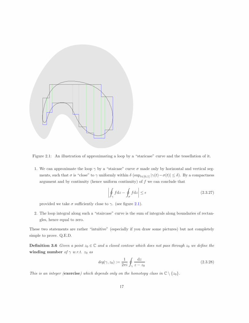
Figure 2.1: An illustration of approximating a loop by a “staricase” curve and the tessellation of it.
1. We can approximate the loop γ by a “staicase” curve σ made only by horizontal and vertical seg-
ments, such that σ is “close” to γ uniformly within δ (supt∈[0,1] |γ(t)−σ(t)| ≤ δ). By a compactness
argument and by continuity (hence uniform continuity) of f we can conclude that∣∣∣∣∮
γ
fdz −∮
σ
fdz
∣∣∣∣ ≤ ǫ (2.3.27)
provided we take σ sufficiently close to γ. (see figure 2.1).
2. The loop integral along such a “staircase” curve is the sum of integrals along boundaries of rectan-
gles, hence equal to zero.
These two statements are rather “intuitive” (especially if you draw some pictures) but not completely
simple to prove. Q.E.D.
Definition 3.6 Given a point z0 ∈ C and a closed contour which does not pass through z0 we define the
winding number of γ w.r.t. z0 as
deg(γ, z0) :=1
2πi
∮
γ
dz
z − z0(2.3.28)
This is an integer (exercise) which depends only on the homotopy class in C \ z0.
17
4 Cauchy’s integral formula
Theorem 2.4.0 Let f(z) be holomorphic on the domain D and let K ⊂ D be a simply connected domain
such that K is compact and ∂K is piecewise smooth; then, for any z ∈ K we have
1
2πi
∮
∂K
f(w)dw
w − z= f(z) (2.4.1)
Proof. Since the integrand is a closed one-form in K \ z and the domain K is simply connected,
we use a homotopy equivalence with a small circle centered at z, Cǫ(z) := |w − z| = ǫ (oriented
counterclockwise).
1
2πi
∮
∂K
f(w)dw
w − z=
1
2iπ
∮
Cǫ(z)
f(z) + f ′(z)(w − z) + o(|w − z|)w − z
dw (2.4.2)
The first term gives the desired result, the second is identically zero and the third is estimated
∣∣∣∣∣1
2iπ
∮
Cǫ(z)
o(|w − z|)w − z
dw
∣∣∣∣∣ ≤ o(1)ǫ. (2.4.3)
Since the result is independent of ǫ, we may send it to zero, thus proving the theorem. Q.E.D.
The theorem can be extended to non simply connected domains and also relaxing the holomorphicity
requirement on the boundary to plain continuity. Specifically
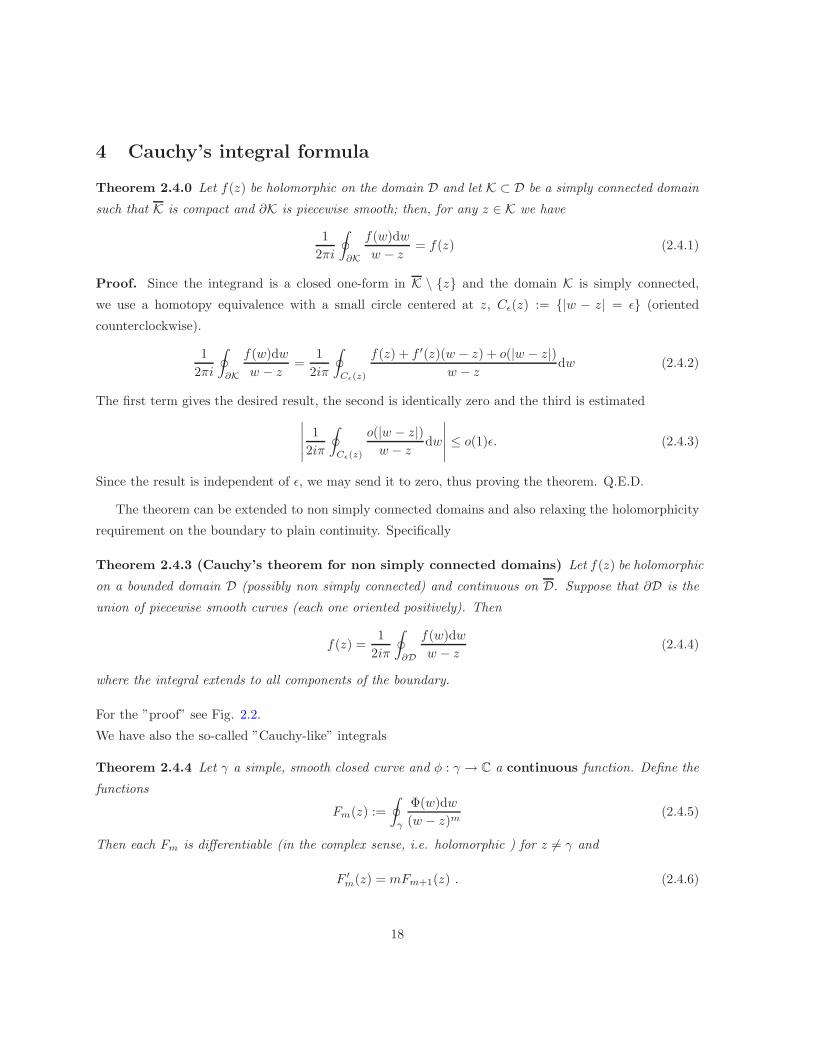
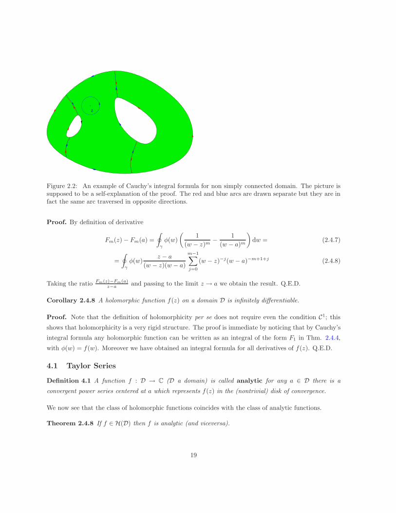
Theorem 2.4.3 (Cauchy’s theorem for non simply connected domains) Let f(z) be holomorphic
on a bounded domain D (possibly non simply connected) and continuous on D. Suppose that ∂D is the
union of piecewise smooth curves (each one oriented positively). Then
f(z) =1
2iπ
∮
∂D
f(w)dw
w − z(2.4.4)
where the integral extends to all components of the boundary.
For the ”proof” see Fig. 2.2.
We have also the so-called ”Cauchy-like” integrals
Theorem 2.4.4 Let γ a simple, smooth closed curve and φ : γ → C a continuous function. Define the
functions
Fm(z) :=
∮
γ
Φ(w)dw
(w − z)m(2.4.5)
Then each Fm is differentiable (in the complex sense, i.e. holomorphic ) for z 6= γ and
F ′m(z) = mFm+1(z) . (2.4.6)
18
z
Figure 2.2: An example of Cauchy’s integral formula for non simply connected domain. The picture issupposed to be a self-explanation of the proof. The red and blue arcs are drawn separate but they are infact the same arc traversed in opposite directions.
Proof. By definition of derivative
Fm(z) − Fm(a) =
∮
γ
φ(w)
(1
(w − z)m− 1
(w − a)m
)dw = (2.4.7)
=
∮
γ
φ(w)z − a
(w − z)(w − a)
m−1∑
j=0
(w − z)−j(w − a)−m+1+j (2.4.8)
Taking the ratio Fm(z)−Fm(a)z−a and passing to the limit z → a we obtain the result. Q.E.D.
Corollary 2.4.8 A holomorphic function f(z) on a domain D is infinitely differentiable.
Proof. Note that the definition of holomorphicity per se does not require even the condition C1; this
shows that holomorphicity is a very rigid structure. The proof is immediate by noticing that by Cauchy’s
integral formula any holomorphic function can be written as an integral of the form F1 in Thm. 2.4.4,
with φ(w) = f(w). Moreover we have obtained an integral formula for all derivatives of f(z). Q.E.D.
4.1 Taylor Series
Definition 4.1 A function f : D → C (D a domain) is called analytic for any a ∈ D there is a
convergent power series centered at a which represents f(z) in the (nontrivial) disk of convergence.
We now see that the class of holomorphic functions coincides with the class of analytic functions.
Theorem 2.4.8 If f ∈ H(D) then f is analytic (and viceversa).
19
Proof. The implication ”analytic⇒ holomorphic” is obvious from Corollary 2.2.10.
Suppose now a ∈ D and let R = dist(a, ∂D). Then for all z ∈ Da(ρ), ρ < R we have
2iπf(z) =
∮
|w−a|=R
f(w)dw
w − z=
∮
|w−a|=R
f(w)dw
w − a− (z − a)=
∮
|w−a|=R
f(w)dw
w − a
1
1 − z−aw−a
= (2.4.9)
=
∮
|w−a|=R
f(w)dw
w − a
∞∑
n=0
(z − a)n
(w − a)n=
M∑
n=0
(z − a)n 2iπ
n!f (n)(a) + RM , (2.4.10)
where
RM :=
∮
|w−a|=R
f(w)dw
w − a
∞∑
n=M+1
(z − a)n
(w − a)n(2.4.11)
The series under the integral sign is majorized in modulus by
|RM (z)| ≤ 2π
(max
w∈|w−a|=R|f(w)|
) ∞∑
n=M+1
( ρR
)n
→ 0 (2.4.12)
as M → ∞. Hence the function is analytic. Q.E.D.
Convergence on the boundary
We only prove a small lemma, but the topic can be a difficult one. Consider a power series: without loss
of generality we assume it centered at z = 0 and with radius of convergence equal to 1 (we can always
reduce to this case with a translation/dilation).
f(z) =∑
cnzn . (2.4.13)
Suppose that the following series converges
∑cneinθ , (2.4.14)
for some value of θ: namely that z = eiθ ∈ ∂D0(1) is a point of convergence. Then
Lemma 2.4.14 If z = eiθ is a point of convergence on the boundary of the disk of convergence for the
series
f(z) =
∞∑
n=0
cnzn , lim sup |cn|
1n = 1 , (2.4.15)
then the function f(z) tends to L :=∑cneinθ when approaching the boundary point from the radial
direction.
Proof. Again we can assume θ = 0 by re-defining cn → cneinθ (i.e. by z 7→ e−iθz). Thus now we have
L =∑cn (convergent) and we want to prove
limx→1−
f(x) = L . (2.4.16)
20
To this end we should estimate
L− f(x) =∑
cn(1 − xn) . (2.4.17)
So we compute
∣∣∣∑
cn(1 − xn)∣∣∣ ≤
∣∣∣∣∣
K∑cn(1 − xn)
∣∣∣∣∣+∣∣∣∣∣∑
K+1
cn(1 − xn)
∣∣∣∣∣ (2.4.18)
Remark 4.1 If we knew thatP
cn is absolutely convergent the conclusion would be easy: letting M = sup |cn|(which is necessarily finite)
˛
˛
˛
˛
˛
KX
cn(1 − xn)
˛
˛
˛
˛
˛
+
˛
˛
˛
˛
˛
X
K+1
cn(1 − xn)
˛
˛
˛
˛
˛
≤ MK
X
(1 − xn) +X
K+1
|cn| ≤ MK2(1 − x) +X
K+1
|cn| (2.4.19)
and the two terms can be made arbitrarily small by taking K large (for the second one) and 1 − x < ǫ/(MK2).
Since∑cn is not absolutely convergent we must ”improve” convergence. This is done by using Abel’s
summation formula ∞∑
M
anbn =∑
M
(an − an+1)
n∑
j=M
bj (2.4.20)
so that
∣∣∣∣∣
K∑cn(1 − xn)
∣∣∣∣∣+∣∣∣∣∣∑
K+1
cn(1 − xn)
∣∣∣∣∣ ≤MK2(1 − x) +
∣∣∣∣∣∣
∑
K+1
(xn − xn+1)
n∑
j=K+1
cj
∣∣∣∣∣∣≤
MK2(1 − x) +∑
K+1
(xn − xn+1)
∣∣∣∣∣∣
n∑
j=K+1
cj
∣∣∣∣∣∣≤MK2(1 − x) + xK+1 sup
n≥K+1
∣∣∣∣∣∣
n∑
j=K+1
cj
∣∣∣∣∣∣≤
≤MK2(1 − x) + supn≥K+1
∣∣∣∣∣∣
n∑
j=K+1
cj
∣∣∣∣∣∣(2.4.21)
Since∑cn is convergent, the last sup tends to zero as K → ∞, hence we can make it less than ǫ/2. The
first term is then less than ǫ/2 for 1 − x < ǫ(2MK(ǫ)2). Q.E.D.
4.2 Morera’s theorem
Morera’s theorem is the ”viceversa” of Cauchy’s theorem
Theorem 2.4.21 (Morera) Let f(z, z) be defined continuous on the domain D and such that for any
closed, simple and D-contractible path γ ⊂ D we have∮
γ
f(z, z)dz = 0 (2.4.22)
Then ∂zf ≡ 0, namely the function is holomorphic.
21
Proof. Consider a disk Da(r) ⊂ D: we prove that f(z, z) is holomorphic in any such disk. Indeed
Fa(z) :=
∫ z
a
f(ξ, ξ)dξ (2.4.23)
is defined in the simply connected disk Da(r) independently of the path of integration. We prove it is
has complex derivative.
1
h(F (z + h) − F (z)) =
1
h
∫ z+h
z
fdζ =1
h
∫ z+h
z
(f(z) + (f(ζ) − f(z))
)dζ = f(z) +Rz(h) (2.4.24)
Rz(h) :=
∫ z+h
z
f(ζ) − f(z)
hdζ (2.4.25)
Since the integration path involved in Rz(h) is irrelevant we take it to be the segment [z, z+ h] and then
we estimate
|Rz(h)| <1
hsup
w∈[z,z+h]
|f(w) − f(z)|L([z, z + h]) = supw∈[z,z+h]
|f(w) − f(z)| (2.4.26)
Since f is continuous on the disk Da(r) ⊂ D it is also uniformly continuous on Da(r − ǫ) and hence
the sup tends to zero as h → 0. This proves that Fa(z) is holomorphic and also that F ′a(z) = f(z, z).
Since we now know that any holomorphic function has also holomorphic derivative, this proves that f is
holomorphic as well. Q.E.D.
5 Maximum modulus and mean value
From now on we denote the set of holomorphic functions on a set B by H(B). We also understand that
if the set B is a closed set, we say that f(z) is holomorphic on B if there exists a domain D containing
B where f(z) is holomorphic.
Definition 5.1 A function f(z) which is holomorphic in C is called entire
We have the following fundamental
Theorem 2.5.0 (Maximum modulus) Let B be a relatively compact domain and f ∈ H(B). Then
the maximum of |f(z)| on B is taken on the boundary ∂B.
Proof. Let
M := supw∈∂B
|f(w)| (2.5.1)
Note that since ∂B is compact and |f(w)| is continuous, the sup is actually a max. We prove that ∀z ∈ B,
|f(z)| ≤M . Indeed let δ = dist(z, ∂B) and note that from Cauchy integral formula we have, ∀n ∈ N that
fn(z) =1
2iπ
∮
∂B
fn(w)dw
w − z(2.5.2)
22
Now,
|fn(z)| ≤ 1
2π
∣∣∣∣∮
∂B
...
∣∣∣∣ ≤L(∂B)Mn
2πδ(2.5.3)
where L(∂ b) denotes the length of a curve1. Continuing, we have
|f(z)| ≤(L(∂B)
2πδ
) 1n
M , ∀n ∈ N (2.5.5)
Taking the limit n→ ∞ yields the result. Q.E.D.
Corollary 2.5.5 If the modulus of a holomorphic function has a local maximum in the interior of the
domain of holomorphicity then f is identically constant.
We first need the
Lemma 2.5.5 If f(z) is holomorphic in a neighborhood of a and |f(z)| is constant, then f(z) is constant.
Proof. If |f(z)| ≡ 0 then there is nothing to prove. So, let |f(z)| = R2 6= 0. We have
f = u+ iv , u2 + v2 = R2 = const . (2.5.6)
Then (by Cauchy-Riemann’s ux = vy , uy = −vx
0 ≡ uux + vvx = uux − vuy (2.5.7)
0 ≡ uuy + vvy = uuy + vux , (2.5.8)
This implies (since the determinant is u2 + v2 = R2 6= 0) that ux ≡ 0 ≡ uy. Similarly for vx, vy, and
hence both u and v are constants. Q.E.D.
Proof of Cor. 2.5.5. Suppose a ∈ D is a local max of |f(z)|. Then there is a disk Da(r) ⊂ D where
a is a global max. Then, for any ρ < r
|f(a)| =
∣∣∣∣∣1
2iπ
∮
|z−a|=ρ
f(z)
z − adz
∣∣∣∣∣ ≤1
2π
∮
|z−a|=ρ
|f(z)|ds ≤ sup|z−a|=ρ
|f(z)| ≤ |f(a)| . (2.5.9)
Note that the second last inequality would be strict as soon as there were a z0 for which |f(z0)| < |f(a)|(by continuity then also in a neighborhood of z0). This proves that |f(z)| = |f(a)| in the whole Da(r),
and hence by the previous lemma is identically constant.
1 Here and also elsewere we use that, if γ is smooth and s is the arclength parameter (and hence x2 + y2 ≡ 1)
˛
˛
˛
˛
Z
γ
f(z)(dx + idy)
˛
˛
˛
˛
=
˛
˛
˛
˛
˛
Z L(γ)
0f(z)(x + iy)ds
˛
˛
˛
˛
˛
≤
Z L(γ)
0|f(z)|ds ≤ sup
z∈γ|f(z)|L(γ) , (2.5.4)
23
Let now M = maxz∈D |f(z)| and let a a point where this max is achieved. Suppose that a is in the
interior of D and consider
M := z ∈ D : |f(z)| = M = |f(a)| . (2.5.10)
This set is a level set of the continuous function |f(z)| and hence it is closed (in the relative topology of
D). Moreover it is nonempty because a ∈ M ⊂ D and –most crucially– it is open. Indeed if b ∈ M then
in particular b is a local max. and by the above f is locally constant in a neighborhood of b, meaning
that a full neighborhood of b belongs to M. Being both open and closed (and non-empty) in a connected
set D then it must coincide with it. Q.E.D.
Corollary 2.5.10 (Liouville’s theorem) An entire function f(z) which is bounded, |f(z)| ≤ M is a
constant
Proof. We prove that f ′(z) ≡ 0. Indeed using Cauchy’s integral formula we have
|f ′(z)| ≤ 1
2π
∮
|w|<R
∣∣∣∣f(w)
(w − z)2dw
∣∣∣∣ ≤M
R(2.5.11)
where R is an arbitrary number |z| < R. Since the result is independent of R we take the limit R → ∞thus concluding that f ′(z) ≡ 0. Q.E.D.
Theorem 2.5.11 (Fundamental Theorem of Algebra) Any nonconstant polynomial P (z) has at least
one zero.
Proof. P (z) is clearly an entire function and if it had no zeroes then 1/P (z) would be a bounded entire
function since actually |P (z)| → ∞ as |z| → ∞ (and hence would be uniformly bounded away from 0),
which can only be a constant. Hence a contradiction. Q.E.D.
5.1 Mean value principle
The first coefficient of the Taylor expansion
f(a) = c0 =1
2πi
∮
|w−a|=ǫ
f(w)dw
w − a=
1
2π
∫ 2π
0
f(a+ reiθ)dθ (2.5.12)
says that
Theorem 2.5.12 The value of a holomorphic function f(z) at any point is the average of the values on
a circle (of arbitrary radius provided it is contained in the domain of holomorphicity).
It is useful to introduce the
24
Definition 5.2 A function f(z) defined and continous on a domain D is said to satisfy the property of
the mean value if ∀a ∈ D and ∀r > 0 such that Da(r) ⊂ D we have
f(a) =1
2π
∫ 2π
0
f(a+ reiθ)dθ (2.5.13)
The theorem of the maximum modulus applies to all functions which satisfy the mean value property
Theorem 2.5.13 (Maximum modulus principle) If f(z) defined and continuous on the domain Dsatisfies the mean value property and is such that |f(z)| has a local maximum at z = a then f(z) is
constant in a neighborhood of a.
Proof. Exercise. Q.E.D.
We can now prove the following lemma which will be used later on
Theorem 2.5.13 (Schwartz’ lemma) Let f ∈ H(|z| < 1) and such that
f(0) = 0, |f(z)| < 1 (2.5.14)
Then
1. We have the inequality
|f(z)| ≤ |z| , ∀z ∈ D0(1) , (2.5.15)
2. If ∃z0 ∈ D0(1), z0 6= 0 such that |f(z0)| = |z0| then f(z) ≡ λz with |λ| = 1.
Proof. Consider the function
g(z) =
f(z)
zz 6= 0
f ′(0) z = 0
(2.5.16)
This is holomorphic in D0(1) since f(0) = 0 By the max. modulus theorem |g(z)| takes on the maximum
on the boundary |z| = 1 or else g(z) is a constant. For any z ∈ D0(1) we haveM(|z|) := sup|w|=|z| |f(w)| <1 by the hypothesis. By the max. modulus theorem
L(|z|) := sup|w|=|z|
|g(z)| =M(|z|)|z| (2.5.17)
is weakly increasing (actually strictly increasing or constant) and supr<1L(r) ≤ 1 since sup |f | ≤ 1.
Therefore |g| ≤ 1 or |f | ≤ |z|. |f(z)| ≤ |z|. The remainder of the proof is left as exercise.Q.E.D
25
6 Laurent series and isolated singularities
Definition 6.1 The point a ∈ C is an isolated singularity for the holomorphic function f(z) if there
is an open neighborhood Ia of a such that f ∈ H(Ia \ a).
Definition 6.2 An isolated singularities is removable if |f(z)| is bounded in a punctured neighborhood
of a.
Proposition 6.1 If a is a removable singularity for f(z) then
1. ∃A := limz→a f(z).
2. The function f(z) defined as f on Ia \ a and f(a) := A is holomorphic in the full neighborhood.
Proof By Cauchy we have
f(z) =1
2πi
∮
|w−a|=R
f(w)dw
w − z− 1
2πi
∮
|w−a|=ǫ
f(w)dw
w − z(2.6.1)
where ǫ < |z − a| < R and both circles are oriented counterclockwise. Since the result is independent of
ǫ and f(w) is bounded we can send ǫ→ 0 and the second integral is easily estimated to tend to zero. At
this point f(z) is a Cauchy integral and hence holomorphic in the vicinity of a as well, where it admits
limit and holomorphic extension. Q.E.D.
In the case where a is not a removable singularity we can use Laurent series.
Laurent series are power series with also negative powers (we consider the case of series centered at z = 0
with the understanding that we could replace z by z − a and obtain analogous expressions centered at
any other point)
f(z) =∑
m∈Z
cnzn =
=:f+(z)︷ ︸︸ ︷∞∑
n=0
cnzn +
=:f−(z)︷ ︸︸ ︷−1∑
n=−∞cnz
n (2.6.2)
The series f+ is a usual power series while the series f− is a series in 1z . We call R+ and 1/R− the
respective radii of convergence. Clearly the expression makes sense as a convergent sum iff R− < R+ and
hence the Laurent series is defined in the annulus
R− < |z| < R+ (2.6.3)
Using these remarks we extend the notion of analyticity to the present context
Definition 6.3 Given a holomorphic function f(z) defined on the annulus R− < |z| < R+ we say that it
admits a Laurent series expansion if there is a convergent Laurent series as above that converges to f(z)
in the same annulus.
26
We leave as exercises the following statements
Lemma 2.6.3 For a function f(z) as in Def. 6.3 the Laurent series -if it exists- is unique and the
coefficients are given by
cn =1
2iπ
∮
|w|=ρ
f(w)
wn+1dw , R− < ρ < R+ . (2.6.4)
Theorem 2.6.4 Every f(z) ∈ H(R− < |z| < R+
)admits expansion in Laurent series.
Note that if only a finite number of cn, n < 0 is nonzero then f− is a polynomial in z−1 and hence R− = 0.
In general we put forward the following
Definition 6.4 We say that z = 0 is a pole of order if M = minn : cn 6= 0 is negative for the
function f(z). If M = −∞ we say that z = 0 is an essential singularity.
Essential singularities have interesting properties;
Theorem 2.6.4 (Sokorskji or Casorati-Weierstrass theorem) Let z = a be an essential singular-
ity for f(z) ∈ H(D); for any punctured disk Da(r)⋆ the values of f on the domain Da(r)⋆ ∩ D is dense
in C.
Proof. Suppose ∃r > 0 such that the values of f(z) taken on the domain I := Da(r)⋆ ∩D is not dense.
Hence ∃F0 ∈ C and ǫ > 0 such that
f(I) ∩DF0(ǫ) = ∅. (2.6.5)
This implies that
g(z) :=1
f(z) − F0(2.6.6)
is bounded in a punctured neighborhood of a and hence can be holomorphically extended there (we use
the same symbol for this extension). Thus
f(z) =1
g(z)+ F0 (2.6.7)
If g(a) 6= 0 then f(z) has no singularity at a, in contradiction with the hypothesis. If g(0) = 0 and the
Taylor series of g(z) starts with a power M then f(z) has a pole of order M at a and not an essential
singularity (note that g(z) is not identically zero and hence at least one coefficient of the Taylor expansion
is nonzero).Q.E.D.
There is a much stronger version of this theorem
Theorem 2.6.7 (Picard’s great theorem) In the same setting of the previous theorem, the set f(Da(r)∩D) is C or the complex plane less a point C \ F0.
Example 6.1 The function f(z) = e1z =
∑0n=−∞
1(−n)!z
n has an essential singularity at z = 0. In any
neighborhood of z = 0 takes on infinitely many times any complex value c
zn(c) =1
ln |c| + i arg(c) + 2iπn(2.6.8)
The exceptional value is c = 0.
27
7 Residues
Exercise 7.1 Prove the following formulæ by explicit parametrization (counterclockwise orientation)
∮
|z−a|=R
dz
(z − a)m=
2iπ m = −10 m ∈ Z ,m 6= −1
(2.7.1)
Definition 7.1 Given an isolated singularity a for a holomorphic function f(z) we define the residue
of f(z) at z = a the coefficient c−1 of the Laurent expansion of f centered at z = a. It can be computed
by the following integral (exercise)
resz=a
f(z)dz :=1
2iπ
∮
|z−a|=ǫ
f(z)dz (2.7.2)
Theorem 2.7.2 (Residues theorem) Let f ∈ H(D \ an) and let an ⊂ D be isolated singularities
for f . Let γ be a simple and contractible closed curve in D and K ⊂ D the ”interior region” of γ (simply
connected). Then ∮
γ
f(z)dz = 2iπ∑
aj∈Kres
z=aj
f(z)dz (2.7.3)
Proof. It is a simple application of Cauchy’s theorem by considering the domain (non-simply connected)
K\⋃aj∈KDaj(ǫ), with ǫ small enough. (You should check that there are only a finite number of isolated
singularities in the compact K).
7.1 Zeroes of holomorphic functions
Let f ∈ H(D) and f not identically zero.
Definition 7.2 If a ∈ D is such that f(a) = 0 we say that f has multiplicity of the zero equal to M
with
M := multa(f) := minn| f (n+1)(a) 6= 0 (2.7.4)
If multa(f) = 1 the zero is said to be simple, otherwise it is multiple. Note that a is a zero of
multiplicity m for an analytic function f(z) iff the Taylor series centered at a (which has positive radius
of convergence) starts with the power m
f(z) = cm(z − a)m + . . . (2.7.5)
Exercise 7.2 Let f(z) be holomorphic in a neighborhood of z = a and suppose that f(a) = 0 (if f(a) = A
we would consider the function F (z) = f(z)−A). Suppose that z = a is a simple zero (i.e. f ′(a) 6= 0):
prove that f(z) admits locally an analytic inverse g(w) such that f(g(w)) = w.
28
Exercise 7.3 Verify that for polynomials, the notion of multiplicity of a zero coincides with the notion
of multiplicity of roots.
Theorem 2.7.5 (Open mapping theorem) The image of a domain D under a holomorphic function
f(z) defined over D is an open set, G := f(D), G =G (where
G denotes the interior of G).
Proof. If w = f(a) and f ′(a) 6= 0 then f(z) is a local homeomorphism between a neighborhood of a and
one of w, which proves that w ∈G. If f(z) − w has a zero of multiplicity M at z = a then the equation
f(z) = b has M distinct solution in a suitable neighborhood of w (exercise). Hence also in this case
w ∈G. Since there are no other possibilities we conclude that G coincides with its interior and hence it
is open. Q.E.D.
7.2 Meromorphic functions
Definition 7.3 A function f is said to be meromorphic on a domain D if there is an at-most-countable2
set of points P := an without accumulation in D such that f is holomorphic on D \ P and the points
an are poles (of finite order).
Exercise 7.4 Prove that the set of meromorphic function over a domain D is a field.
Exercise 7.5 Prove that an isolated singularity z = a for a holomorphic function f(z) is a pole (of finite
order) iff |f(z)| → ∞ as z → a.
7.3 Application of the residue theorem to multiplicities of zeroes
Let f be meromorphic on a domain D; we want to count its zeroes and poles. We first have
Proposition 7.1 The function g(z) = (ln(f(z))′ = f ′(zf(z) is meromorphic in D and the poles are all simple
and located precisely at the zeroes and poles of f(z). The residues of g(z) at one such pole a is
resz=a
f ′(z)
f(z)dz =
m ∈ N \ 0 multiplicity of a if a is a zero of f(z)−m ∈ −N \ 0 order of the pole if a is a pole of f(z)
(2.7.6)
Proof. Consider the Laurent/Taylor series of f(z) at a
f(z) =∑
n≥M
cn(z − a)n (2.7.7)
f ′(z) =∑
n≥M
ncn(z − a)n (2.7.8)
f ′(z)
f(z)=
M
z − a+ O(1) (2.7.9)
Q.E.D.
2This means that the set is either finite or else infinite but countable.
29
Corollary 2.7.9 Let γ be a closed simple curve in D and an be the zeroes of f with multiplicities mn
and bj the poles with orders pj (there is a finite number of either in the region bounded by γ): then
1
2iπ
∮
γ
f ′(z)
f(z)dz =
∑
n
mn −∑
j
pj (2.7.10)
1
2iπ
∮
γ
zf ′(z)
f(z)dz =
∑
n
mnan −∑
j
pjbj (2.7.11)
More generally if g(z) ∈ H(D) then
1
2iπ
∮
γ
g(z)f ′(z)
f(z)dz =
∑
n
mng(an) −∑
j
pjg(bj) (2.7.12)
In other words we can assign a ”charge” to each zero (positive) and pole (negative) and then the above
integrals compute the total charge and the ”center of charge” or (for the last integral) some weighted
sum of any holomorphic function at the sites of the charges.
Exercise 7.6 Prove Corollary 2.7.9.
30
Chapter 3
Applications of complex integration
Most of the statement in this chapter are left as exercise. We use the notion of analytic continuation
which is going to be defined later on, but I hope that you have faint memories of your past undergrad.
course.
First of all we have the following alternative expressions for the residues. Let f(z) have a pole of
order m at z = a then
resz=a
f(z)dz =1
(m− 1)!limz→a
((z − a)mf(z)
)(m−1)
(3.0.1)
In particular for a simple pole we have
resz=a
f(z)dz = limz→a
(z − a)f(z) . (3.0.2)
These formulas follow by direct manipulations of the Laurent series expansion of f around z = a.
Exercise, do it!. One of the most interesting applications of the theorem of residues is in the summation
of series.
1 Summation of series
Consider a series of the form
S :=∞∑
n=−∞f(n) (3.1.1)
where f(z) is a holomorphic function (or meromorphic) such that
|f(z)| = O(|z|−1−ǫ) . (3.1.2)
as |z| → ∞. We find an auxiliary function g(z) which has simple poles at the integers with residue 1,
typically
g(z) =π cos(πz)
sin(πz)= π cot(πz) . (3.1.3)
31
m+1
Qm
m
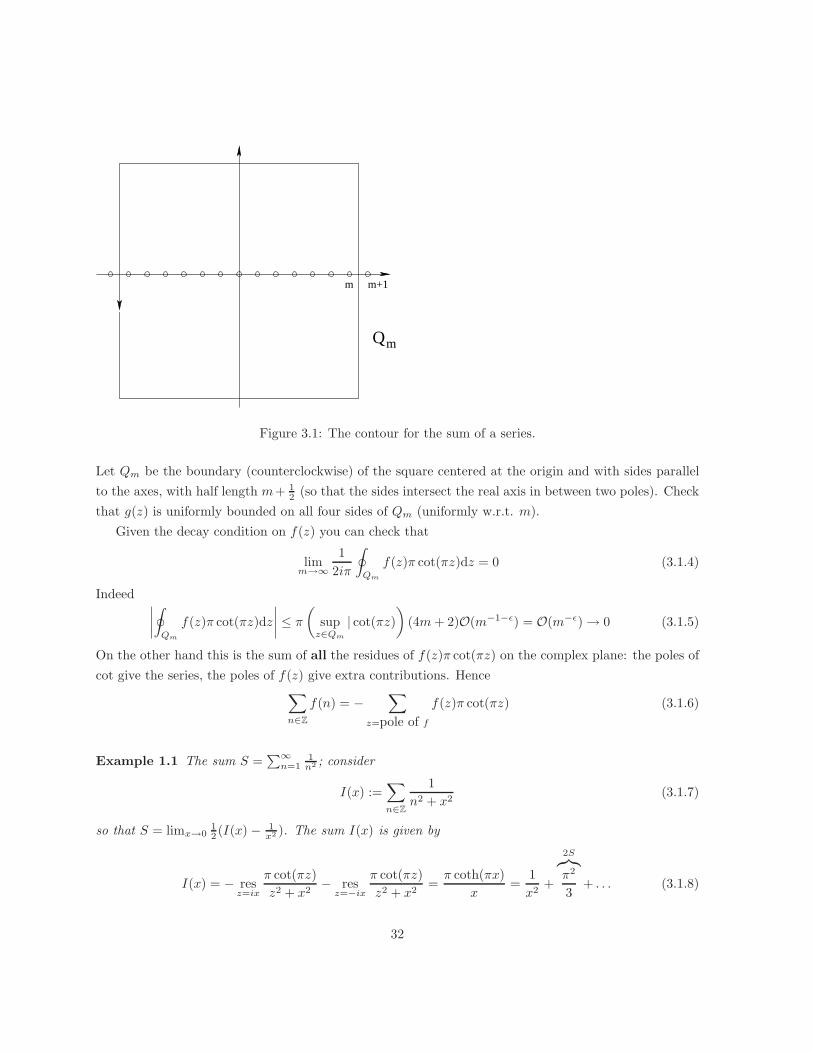
Figure 3.1: The contour for the sum of a series.
Let Qm be the boundary (counterclockwise) of the square centered at the origin and with sides parallel
to the axes, with half length m+ 12 (so that the sides intersect the real axis in between two poles). Check
that g(z) is uniformly bounded on all four sides of Qm (uniformly w.r.t. m).
Given the decay condition on f(z) you can check that
limm→∞
1
2iπ
∮
Qm
f(z)π cot(πz)dz = 0 (3.1.4)
Indeed ∣∣∣∣∮
Qm
f(z)π cot(πz)dz
∣∣∣∣ ≤ π
(sup
z∈Qm
| cot(πz)
)(4m+ 2)O(m−1−ǫ) = O(m−ǫ) → 0 (3.1.5)
On the other hand this is the sum of all the residues of f(z)π cot(πz) on the complex plane: the poles of
cot give the series, the poles of f(z) give extra contributions. Hence∑
n∈Z
f(n) = −∑
z=pole of f
f(z)π cot(πz) (3.1.6)
Example 1.1 The sum S =∑∞
n=11
n2 ; consider
I(x) :=∑
n∈Z
1
n2 + x2(3.1.7)
so that S = limx→012 (I(x) − 1
x2 ). The sum I(x) is given by
I(x) = − resz=ix
π cot(πz)
z2 + x2− res
z=−ix
π cot(πz)
z2 + x2=π coth(πx)
x=
1
x2+
2S︷︸︸︷π2
3+ . . . (3.1.8)
32
For alternating series use instead of cot the function
g(z) =π
sin(πz), (3.1.9)
which has residues at the integers equal to (−1)n. Usually one first needs to ”double” the series in
question by writing as sum over all Z instead of just N, as in the example above.
1.1 Fourier series
Consider series of the form
F (ω) :=∑
n∈Z
f(n)eiωn (3.1.10)
Then we use a similar strategy with
g(z) =2iπ
e2iπz − 1(3.1.11)
so that
F (ω) =∑
x∈R, x= pole
resz=x
f(z)2iπeizω
e2iπz − 1(3.1.12)
2 Integrals
2.1 Case 1
Improper integrals of the form
I :=
∫ ∞
0
f(x)√xdx (3.2.1)
where f(z) is meromorphic on C. Take the contour Γ(R) consisting of the segment [ 1R , R] followed by
the circle of radius R followed by [R, 1R ] and the circle of radius 1
R . In the limit R → ∞ the two small
circles can be discarded if
|f(z)| = o(|z|− 32−ǫ) , z → 0|f(z)| = o(|z| 32+ǫ) , z → ∞. (3.2.2)
and we have (remember that after analytic continuation√z changes sign.)
2I = 2iπ∑
poles6=0
reszf(z)
√zdz (3.2.3)
33
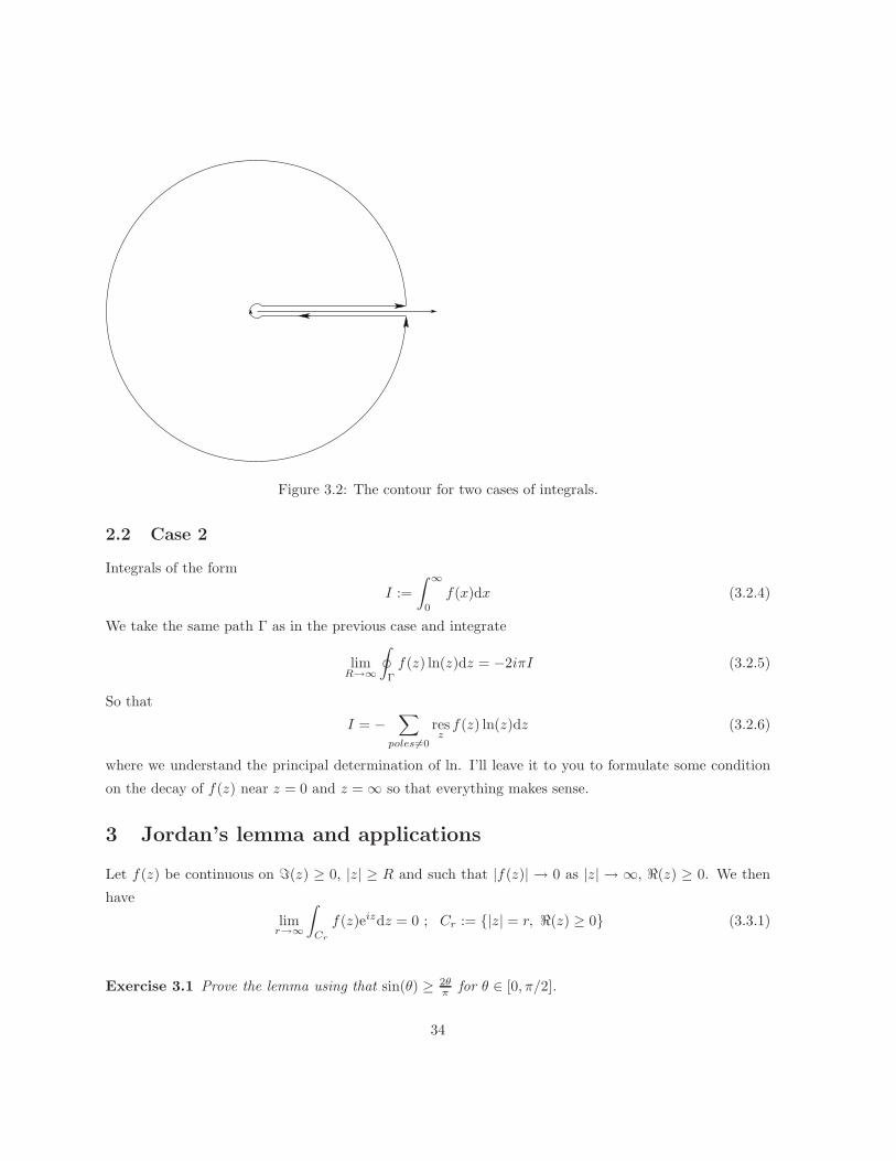
Figure 3.2: The contour for two cases of integrals.
2.2 Case 2
Integrals of the form
I :=
∫ ∞
0
f(x)dx (3.2.4)
We take the same path Γ as in the previous case and integrate
limR→∞
∮
Γ
f(z) ln(z)dz = −2iπI (3.2.5)
So that
I = −∑
poles6=0
reszf(z) ln(z)dz (3.2.6)
where we understand the principal determination of ln. I’ll leave it to you to formulate some condition
on the decay of f(z) near z = 0 and z = ∞ so that everything makes sense.
3 Jordan’s lemma and applications
Let f(z) be continuous on ℑ(z) ≥ 0, |z| ≥ R and such that |f(z)| → 0 as |z| → ∞, ℜ(z) ≥ 0. We then
have
limr→∞
∫
Cr
f(z)eizdz = 0 ; Cr := |z| = r, ℜ(z) ≥ 0 (3.3.1)
Exercise 3.1 Prove the lemma using that sin(θ) ≥ 2θπ for θ ∈ [0, π/2].
34
As application, if f(z) is meromorphic in ℑ(z) > 0 and continuous in ℑ(z) ≥ 0, such that |f(z)| → 0 as
|z| → ∞, ℑ(z) ≥ 0, then
∫ ∞
−∞f(x)eixdx = 2iπ
∑
aj=pole of f
resz=aj
f(z)eiz . (3.3.2)
Exercise 3.2 Compute
∫ ∞
−∞
(x− 1)eix
x2 − 2x+ 2dx (3.3.3)
∫
R
cos(x)
(x2 + 2ix− 2)2dx (3.3.4)
etc.etc.
35
Chapter 4
Analytic continuation
1 Analytic continuation
Lemma 4.1.0 Let f ∈ H(D) and a ∈ D such that f(a) = 0; the following statements are mutually
exclusive:
(a) There exists a neighborhood Ua of a such that f(z) ≡ 0, ∀z ∈ Ua;
(b) There exists a neighborhood Ua of a such that f(z) 6= 0, ∀a 6= z ∈ Ua.
Proof. Let f(z) =∑∞
n=0 cn(z − a)n be the Taylor series of f with radius of convergence R > 0. Let M
be the order of the zero, i.e. M = minn : cm 6= 0. We assume M < ∞, namely the series is not
identically zero, for otherwise we are in situation (a). Consider
g(z) =f(z)
(z − a)M. (4.1.1)
This function is analytic at z = a and g(a) 6= 0: hence -by continuity- there is a neighborhood of a where
g(z) is never zero. Therefore f(z) = (z − a)Mg(z) is not zero in this punctured neighborhood of z = a.
Q.E.D.
Corollary 4.1.1 If the zeroes of f ∈ H(D) accumulate in the interior of D then f(z) is identically zero
on D.
Proof. If this would happen then an accumulation point z0 ∈ D would also be a zero of f(z) (by
continuity). Then, by Lemma 4.1.0 f(z) is zero on an open neighborhood of z = a. Consider now the set
Z(f) := z ∈ D : , ∃ǫ > 0 : f(Dz(ǫ)) = 0 . (4.1.2)
(The set of ”fat” zeroes). The definition implies that Z(f) is open and we have just proved that it is not
empty since z0 belongs to it. By continuity of f(z) the set Z(f) is closed since a point z1 of accumulation
36
for Z(f) has the property contradicting (a) of Lemma 4.1.0, and hence belongs to Z(f). Since Z(f) is
open and closed, then -by elementary topological properties of connected sets- Z(f) = D. Q.E.D.
The above lemma and corollary constitute the principle of analytic continuation, stating that
Corollary 4.1.2 Let f, g ∈ H(D). Suppose ∃a ∈ D and an infinite set G with a as accumulation point
such that f(z) = g(z), ∀z ∈ G: then f ≡ g on D. In particular if f = g on any open disk then they are
equal on the whole D.
Definition 1.1 The pair (B, f) where B is a domain and f ∈ H(B) is called an analytic element. We
say that the analytic element (B, f) is an analytic continuation of an analytic element (B, f) if B ⊃ Band f ≡ f on B.
It is clear that two analytic continuations of an analytic element must coincide on the intersection of the
respective domains (in view of our (4.1.0)).
Corollary 4.1.2 Let (B, f) be an analytic element and B ⊃ B: let f1, f2 ∈ H(B) two analytic continu-
ations of (B, f). Then f1 = f2.
In other words, if an analytic continuation exists, it is unique.
Definition 1.2 Given a ∈ C we define an equivalence relation Ra between all analytic elements (D, g)
such that a ∈ D: two analytic elements (B, f) and (D, g) are equivalent if a ∈ B ∩ D and f ≡ g in a
neighborhood of a, Ua ⊂ B ∩ D. The equivalence classes are called germs of analytic functions at
z = a and denoted by [f ]a.
It is clear that germs of analytic functions at a are in one-to-one correspondence with convergent power
series centered at a.
We finally define the analytic continuation of a (germ of ) analytic element along a path.
Definition 1.3 Let (B, f) be an analytic element and γ : [0, 1] → C such that γ(0) ∈ B. The analytic
continuation of f along γ is a family (Bt, ft) of analytic elements such that
1. [f ]γ(0) = [f0]γ(0)
2. γ(t) ∈ Bt
3. ∀t ∈ [0, 1] ∃δ > 0 such that |s− t| < δ implies γ(s) ∈ Bt
4. [ft]γ(s) = [fs]γ(s).
We say also that (B1, f1) is the analytic continuation of (B0, f0) along the given path.
The following Lemma holds (without the nondifficult proof)
37
Lemma 4.1.2 Given a curve γ : [0, 1] → C connecting the points γ(0) = a to γ(1) = b and two analytic
continuations of analytic elements (Bt, ft) and (Dt, gt) such that the initial germs coincide [f0]a = [g0]a
then so do all germs
[ft]γ(t) = [gt]γ(t) . (4.1.3)
This lemma implies that what we actually continue are germs of analytic functions.
Definition 1.4 The complete analytic function (in Weierstrass’ sense) of an analytic element (B, f)
is the collection of all germs [g]b for which there is a point a ∈ B and a path γ connecting a to b such
that [g]b is the continuation of the germ [f ]a along γ.
Example 1.1 Consider the function ln(z) : ℜ(z) > 0 → C, defined as
ln z :=
∫ z
1
dξ
ξ. (4.1.4)
Such function has the properties of the usual logarithm since
eln(z) = z (4.1.5)
which can be verified by taking the derivative of both sides and comparing the values at z = 1. Explicitly
we know that
ln(z) = ln |z| + i arg(z) , (4.1.6)
where in the RHS ln means the usual logarithm of real numbers and here the argument is chosen in
(−π/2, π/2). Here it is ”simple” to see what is the analytic continuation of ln(z) along the counterclock-
wise circle centered at z = 0 and radius 1; the result will be the germ of an analytic function ln(z) at
z = 1 such that
ln(z) = ln(z) + 2iπ (4.1.7)
in a suitable neighborhood of z = 1. Viceversa, analytic continuation in the clockwise orientation will
produce a different germ
ln(z) = ln(z) − 2iπ . (4.1.8)
Exercise 1.1 Consider the function
f(z) = |z|1/2ei arg(z)/2 ,ℜ(z) > 0. (4.1.9)
Describe the complete analytic function of this analytic element, which we will call√z.
38
s
t
R(t)
R(s)
γ( )γ( )
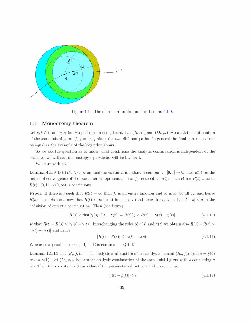
Figure 4.1: The disks used in the proof of Lemma 4.1.9.
1.1 Monodromy theorem
Let a, b ∈ C and γ, γ be two paths connecting them. Let (Bt, ft) and (Dt, gt) two analytic continuation
of the same initial germ [f0]a = [g0]a along the two different paths. In general the final germs need not
be equal as the example of the logarithm shows.
So we ask the question as to under what conditions the analytic continuation is independent of the
path. As we will see, a homotopy equivalence will be involved.
We start with the
Lemma 4.1.9 Let (Bt, ft)γ be an analytic continuation along a contour γ : [0, 1] → C. Let R(t) be the
radius of convergence of the power series representation of ft centered at γ(t). Then either R(t) ≡ ∞ or
R(t) : [0, 1] → (0,∞) is continuous.
Proof. If there is t such that R(t) = ∞ then ft is an entire function and so must be all fs, and hence
R(s) ≡ ∞. Suppose now that R(t) < ∞ for at least one t (and hence for all t’s). Let |t − s| < δ in the
definition of analytic continuation. Then (see figure)
R(s) ≥ dist(γ(s), |z − γ(t)| = R(t)) ≥ R(t) − |γ(s) − γ(t)| (4.1.10)
so that R(t)−R(s) ≤ |γ(s)− γ(t)|. Interchanging the roles of γ(s) and γ(t) we obtain also R(s)−R(t) ≤|γ(t) − γ(s)| and hence
|R(t) −R(s)| ≤ |γ(t) − γ(s)| (4.1.11)
Whence the proof since γ : [0, 1] → C is continuous. Q.E.D.
Lemma 4.1.11 Let (Bt, ft)γ be the analytic continuation of the analytic element (B0, f0) from a = γ(0)
to b = γ(1). Let (Dt, gt)ρ be another analytic continuation of the same initial germ with ρ connecting a
to b.Then there exists ǫ > 0 such that if the parametrized paths γ and ρ are ǫ close
|γ(t) − ρ(t)| < ǫ (4.1.12)
39
the final germs coincide [f1]b = [g1]b. (Invariance of the analytic continuation under small perturbations
of the path).
Proof. We define R(t) as in Lemma 4.1.9. If R(t) ≡ ∞ any ǫ will suffice and the proof is left as exercise.
Suppose R(t) < ∞. Since it is continuous on a compact, it has a positive minimum. We take ǫ as half
of this minimum. This guarantees that ρ(t) is always within the disk of convergence of the power series
representation of ft. Without loss of generality we assume that Bt and Dt are the respective disks of
convergence of the p.s. reps. of ft and gt. Consider the set
T := t ∈ [0, 1] s.t. ft(z) ≡ gt(z) , ∀z ∈ Bt ∩Dt (4.1.13)
Such set is nonempty since by assumption t = 0 ∈ T . We prove that it is open and closed in [0, 1]
and connectivity of the interval will conclude that T = [0, 1]. In particular f1 and g1 coincide in a
neighborhood of z = b and hence define the same germ. To prove that it is open we take a neighborhoot
U of t ∈ T such that ∀t′ ∈ U we have
|γ(t) − γ(t′)| < ǫ
2and |ρ(t) − ρ(t′)| < ǫ
2. (4.1.14)
We now show that γ(t′) belongs to Dt′ and symmetrically that ρ(t′) ∈ Bt′ . Indeed
|γ(t′) − ρ(t′)| ≤ |γ(t′) − γ(t)| + |γ(t) − ρ(t)| + |ρ(t) − ρ(t′)| ≤ 2ǫ ≤ R(t). (4.1.15)
Therefore γ(t′) and ρ(t′) belong to Dt∩Dt′ ∩Bt∩Bt′ and hence all power series reps of ft, ft′ , gt, gt′ have
a nonempty common intersection of the respective disks. Thus we have the equality of ft′(z) ≡ gt′(z),
z ∈ Dt ∩Dt′ ∩Bt ∩Bt′ and hence T is open.
We prove now that T is closed hence concluding the proof. Let t0 be an accumulation point of T : as
above
∃t s.t. |γ(t) − γ(t0)| <ǫ
2and |ρ(t) − ρ(t0)| <
ǫ
2. (4.1.16)
As before one has that the fourtuple intersection of the disks of convergence is nonempty (and open) so
t0 belongs to T as well and T is closed. Q.E.D.
Definition 1.5 An analytic element (B, f) admits unrestricted analytic continuation to the domain
D ⊃ B if for any path γ ⊂ D with initial point in B there exists an anlytic continuation of (B, f) along
γ.
Theorem 4.1.16 Let D be a domain where the analytic element (B, f) can be unrestrictedly analytically
continued. Let γ1, γ2 ⊂ D be curves D-homotopic at fixed end-points. Then the analytic continuations of
(B, f) along γ1, γ2 yield the same germ of analytic function at γ1(1) = γ2(1).
40
Corollary 4.1.16 If D above is simply connected then there is an analytic function F : D → C such that
F|B ≡ f .
Example 1.2 The domain D where (ℜ(z) > 0, ln(z)) admits unrestricted analytic continuation is
C× = C \ 0. However there is no analytic function F (z) defined on C× which restricts to ln(z) on
ℜ(z) > 0. If this where the case the analytic continuation of ln(z) around the origin counterclockwise or
clockwise would yield the same result, which is not the case.
Exercise 1.2 Prove Corollary 4.1.16.
2 Schwartz reflection principle
This is a particularly useful application of analytic continuation
Theorem 4.2.0 Let D+ a domain in the upper half plane ℑ(z) > 0 such that I := D+∩R 6= ∅ is a union
of intervals. Suppose f(z) is holomorphic on D+ and continuous on D+ and also f(x) ∈ R , ∀x ∈ I ⊂ R.
Then there exists a holomorphic function g defined on D+ ∪D∗+ such that g|D+
= f .
Proof. We define
g(z) =
f(z) z ∈ D+
f(z) z ∈ D− := D+∗ (4.2.1)
Such function is also continuous on I. Since it can be represented as a Cauchy integral on a contour
embracing subintervals of I it is also holomorphic at points of I. Q.E.D.
41
Chapter 5
One-dimensional complex manifolds
We begin with some general facts about topological spaces and differential geometry.
1 Definition
Definition 1.1 A (real/complex) manifold of dimension n is a set M with a collection of pairs (Uα, φα)α∈A
where Uα ⊂M and φα : Uα → (R/C)n on their respective images and such that
1. φα(Uα) is open in [R/C]n and φα : Uα → φα(Uα) is one-to-one.
2. The sets Uα are a covering of M ⋃
α∈AUα = M (5.1.1)
3. If Uα,β := Uα ∩ Uβ 6= ∅ then both φα(Uα,β) and φβ(Uα,β) are open and
Gα,β := φα φ−1β : φβ(Uα,β) → φα(Uα,β) (5.1.2)
are (Ck/analytic) functions of all the respective variables.
The maps φα are called local coordinates, the sets Uα are called local charts. The functions Gα,β are
called transition functions.
Given two collections of local coordinate-charts φα, Uαα and ψβ , Vββ, we say that they are equivalent
if their union still defines a (real/complex) manifold structure. The equivalence classes of local coordinate-
charts [(Uα, φα)α] are called atlases (or conformal structure in the complex case).
Note that –interchanging α ↔ β in the last point of the definition– we have that Gα,β are invertible
and the inverse is in the same class (Ck or analytic), G−1α,β = Gβ,α.
A complex n-dimensional manifold is also a real C∞ manifold of dimension 2n. We will be concerned
with manifold of complex dimension 1 and hence the local charts zα = φα(p) will be complex valued
42
functions providing local identification of M with a domain in C. The set M becomes immediately a
topological space with the topology inherited via φ−1α from [R/C]n; an open set U in M is a set such that
φα(U) is open ∀α.
From now on we restrict the formulation to complex one–dimensional manifolds, but many definitions
and statements are obvious specializations of more general ones where either we have more dimensions
or we change the ” category” of functions from ”analytic” (holomorphic) to Ck or else.
Definition 1.2 Let M be a complex one-dimensional manifold with atlas (Uα, zα). A function f :
M → C is said to be holomorphic (meromorphic) if for each local chart we have
f φ−1α : φα(Uα) → C
zα 7→ fα(zα) := f(φ−1α (zα))
(5.1.3)
is holomorphic/meromorphic on the open set φα(Uα)).
Note that on the intersection of charts Uα,β the notion of holomorphicity/meromorphicity in the different
coordinates is the same since the transition functions are biholomorphic.
Theorem 5.1.3 Let M be connected and compact in the topology of the atlas. Then the only holomorphic
functions are constants.
Proof. Since |f | is continuous on the compact M then it takes on a maximum at p ∈ M . Let p ∈ Uα,
then fα has a maximum modulus in the interior of φα(Uα) and hence it is constant on Uα. Let q ∈ M
and since M is connected it is also arcwise connected (exercise). Let γ be a continuous path from p to
q: by compactness of γ it can be covered by a finite number of charts Uαj, with Uα0 = Uα. By induction
you can show that fαk≡ C ⇒ fαk+1
≡ C and hence fαN= C = fα0 . Q.E.D.
Definition 1.3 Let M and N be two complex one-dimensional manifolds with atlases respectively (Uα, φα)
and (Vβ , ψβ). We say that a map
ϕ : M → N (5.1.4)
is holomorphic if at any point p ∈M , p ∈ Uα, ϕ(p) ∈ Vβ then wβ = ψβ(f(φ−1α (zα) is holomorphic in a
small disk arount φα(p).
Remark 1.1 It is customary to abuse the notation and identify a point p ∈ Uα with its coordinate zα = zα(p) :=φα(p). The above function then would be written as wβ = f(zα).
Definition 1.4 Two complex manifolds M,N are biholomorphic (or biholomorphically equiva-
lent) if there exist two holomorphic bijections ϕ : M → N and ψ : N → M such that ϕ ψ = IdN and
ψ ϕ = IdM . This defines an equivalence relation (exercise).
When considering complex manifolds we do not distinguish between manifolds which are biholomorphi-
cally equivalent and hence we re-define a complex manifold to be the equivalence class of complex
manifolds (as in the former definition).
43
Definition 1.5 A holomorphic map ϕ : M → M which admits holomorphic inverse is called auto-
biholomorphism or automorphism (for short). The set of automorphisms of a (complex) manifold M
will be denoted by Aut(M) and it is a group with respect to the composition of maps.
2 One-forms and integration
We always assume that
(M, (Uα, φα)α
)is a complex one-dimensional variety with atlas of charts
zα = zα(p) = φα(p). Instead of introducing the abstract notion of tangent and cotangent space (which
would be the ”comme-il-faut” way) we give a ”hands-on” definition of forms.
Definition 2.1 A [holomorphic/meromorphic] one form ω is a collection of functions fα : Uα → C
which are [holomorphic/meromorphic] in the local chart zα and such that on the intersection Uα ∩Uβ we
have
fα = fβdzβ
dzα(5.2.1)
Here the notationdzβ
dzαmeans the Jacobian of the function zβ(zα) = φβ(φ−1
α (zα). and we tacitly under-
stand that we will think of the fα’s as functions either of the abstract point p ∈ M or as ”concrete”
functions of the local coordinate zα as most convenient for the context and without explicit mention.
If we treat the symbols dzα formally then the mnemonics behind the definition is
fαdzα = fβdzβ , (5.2.2)
on the intersection, and hence the reference to the chart becomes irrelevant.
A particular class of one-forms are differentials: given a [holomorphic/meromorphic] function f : M →C we define its differential df as the one form given in local coordinates by
df = f ′(zα)dzα . (5.2.3)
As a consequence of the chain-rule this definition does provide a differential in the sense specified above.
The use of one-forms is -as always- that of being integrated alont one-dimensiona real manifolds,
namely curves. A curve is simply a map γ : [0, 1] → M which is continuous. The notion of smoothness
Ck is easy to formulate and it is left as exercise.
If the whole support of a curve γ lies within a single coordinate chart then integration of a one–form
ω along the curve is defined as in the complex plane using the local coordinate. Some care should be
paid (but ”only the first time you do it”) to define it consistently when the support of γ extends to more
than one chart.
44
Integration of one-forms along curves Let ω be a [holomorphic/meromorphic] one–form and γ :
[0, 1] →M be a continuous curve. We define the integral of ω along γ∫
γ
ω (5.2.4)
as follows. Let Uj be a covering of γ by charts. By compactness we can take it finite and we can order it
so that Uj ∩Uj+1 6= ∅. We take points tj such that γ(tj) ∈ Uj ∩Uj+1. By construction the arc γ([tj , tj+1])
lies within a single chart Uj+1 and then we define∫
γ
ω =∑
j
∫ tj+1
tj
fj+1(zj+1(t))zj+1(t)dt . (5.2.5)
One should then prove that the definition is independent of the choice of the splitting points. This follows
from the following exercise.
Exercise 2.1 Let γ := [a, b] → Uα ∩ Uβ and let ω be a one form: prove that
∫ b
a
fα(zα(t))zα(t)dt =
∫ b
a
fβ(zβ(t))zβ(t)dt (5.2.6)
(The notation zα(t) is a short-hand for zα(γ(t)) = φα(γ(t))).
We also need the generalization of Stokes’ theorem. To this end we must define two–forms
Definition 2.2 A two–form η is a collection of smooth-functions gα(xα, yα) of the real variables xα =
ℜ(zα), yα = ℑ(zα) such that
gα = gβ det
(∂xβ
∂xα
∂xβ
∂yα
∂yβ
∂xα
∂yβ
∂yα
)= gβ
∣∣∣∣dzβ
dzα
∣∣∣∣2
(5.2.7)
As before the mnemonics is
− 2igαdxα ∧ dyα = gαdzα ∧ dzα = 2igβdxβ ∧ dyβ = gβdzβ ∧ dzβ (5.2.8)
The reason of the definition is that now we can integrate η over a domain (open connected set) D ⊂ M
which may extend over several charts. Suppose now we have a non-holomorphic one form, i.e.
ω = fαdzα + fαdzα (5.2.9)
where the functions fα, fα are defined such that
fα = fβdzβ
dzα, fα = fβ
dzβ
dzα(5.2.10)
but in general we admit that f, f are not holomorphic. The total differential is defined as earlier in the
course to be the two-form given in local coordinates
dω =(∂zα
fα − ∂zαfα
)dzα ∧ dzα (5.2.11)
We then have
45
Theorem 5.2.11 Let D a domain in M and ω a one form defined and smooth over D. Then∫
∂Dω =
∫ ∫
Ddω . (5.2.12)
In particular if ω is a meromorphic one form and D does not include any of the poles then∫
∂D ω = 0
since dω is smooth and identically zero on D.
2.1 Zeroes and poles: residues
In general it makes no sense to talk about the value of a one-form at a point because the function fα
depends on the local coordinate: if we re-define the local coordinate wα = Wα(zα) by a biholomporphic
function Wα then we have
fα = fαdWα
dzα(5.2.13)
and the value will change. Ditto for points in the intersection of different charts. However it p ∈ M is
such that fα(p) = 0 then the same holds in any local coordinate. Similarly if p is a pole and hence fα has
a pole at zα(p) then so it must be for all coordinates whose charts cover the point p and for all other local
coordinate we can choose on the given chart. Even more, if p is a zero/pole of ω, its multiplicity/order
is independent of the choice of coordinate. This motivates the following
Definition 2.3 Let ω be a [holomorphic/meromorphic] one form on M . We say that p ∈ M is a
zero/pole of ω of multiplicity/order m if fα(zα) has a zero/pole of the same multiplicity/order at zα(p).
Exercise 2.2 Prove that if we change local coordinate w = W (zα) in a neighborhood of zα(p) the notion
multiplicity/order of the zero/pole does not change. Prove the same also if p lies in the intersection of
different charts.
Residues
Let ω be a meromorphic one–form and p a pole. Let z = zα be a local chart covering p and a = zα(p).
Then (denoting f(z) = fα(zα))
ω = f(z)dz =∑
n≥−M
cn(z − a)ndz (5.2.14)
is the local Laurent series expansion.
Definition 2.4 The residue of ω at p is
respω = c−1 (5.2.15)
where c−1 is defined by the local expansion (5.2.14).
46
Note that the coefficients cn depend on the choice of coordinate and that c−1 is the only one which does
not. In order to see this we can note that
c−1 =1
2iπ
∮
|zα−a|=ǫ
fα(zα)dzα =1
2iπ
∮
γǫ
ω (5.2.16)
where γǫ is a small loop around p in M . Since the integral of the one–form is independent of the
coordinate, then so is c−1.
Exercise 2.3 Verify directly on the Laurent expansion that c−1 is independent of the local coordinate.
One-forms on a complex one–dimensional manifold are customarily classified in three kinds.
Definition 2.5 A one form ω on M is called of the first kind if it is holomorphic, of the second kind
if it is meromorphic but the residues at all poles are zero, and of the third kind if at least one residue
is non-zero.
We have however the following
Theorem 5.2.16 Let M be a compact complex curve (=one–dimensional manifold≡ two-dimensional
real surface). Let ω be a meromorphic one–form. Then the sum of all residues is zero
∑
p=pole of ω
respω = 0 (5.2.17)
Proof. We take the domain D = M \⋃p= poles of ω Dp(ǫ) where Dp(ǫ) stands for small disks centered at
p (in a local coordinate). Then the sum of residues is precisely (minus) the integral of ω on the boundary
∂D ∑
p=pole of ω
respω = −
∫
∂Dω = −
∫ ∫
Ddω = 0 (5.2.18)
by Stokes’ theorem. Q.E.D.
Exercise 2.4 Let f : M → C be a meromorphic function with only one simple pole. Prove that this
establishes a biholomorphic equivalence with the Riemann–Sphere.
[Hint; apply the residue theorem to dff−a , a ∈ C]
3 Coverings and Riemann surfaces
Definition 3.1 Given a one-dimensional complex manifold N , a Riemann surface over N is a pair
(M, f) where M is another one-dimensional complex manifold and f : M → N is a holomorphic map
onto.
Definition 3.2 The map f : M → N is called univalent if f(a) 6= f(b) for a 6= b.
47
The local description of univalent maps is easy. Let a ∈ M and A = f(a). We take local coordinates z
and w in a neighborhood of a and A and we can assume that z(a) = 0, w(A) = 0 (we may have to shift
the coordinates supplied with the atlas and redefine them). Then we can think of f restricted to the
chart of z as a holomorphic function of z
f ∈ H(D0(ǫ)) , w = f(z) , f(0) = 0 . (5.3.1)
The condition of local univalency translates in f ′(0) 6= 0.
More generally, for holomorphic maps f : M → N we introduce the following
Definition 3.3 A point a ∈M is called a ramification point if, in local coordinates a and w centered
at a and A = f(a) respectively, we have f ′(z)|z=z(a) = 0. The point A ∈ N is called branchpoint. The
multiplicity of the zero of f ′(z) at z = z(a) is called the index of ramification (and it is independent of
the choiche of local coordinates). A map f : M → N for which there are no ramification points is called
unramified.
Example 3.1 The map exp : C → C×, exp(z) := e2iπz is unramified but not univalent.
We have the extension of the open-mapping theorem, whose proof is virtually identical and left as
exercise.
Lemma 5.3.1 Let D ⊂ M be a domain (=open and connected set). Then the image f(D) ⊂ N under
a non-constant holomorphic map is open as well (and connected, hence a domain).
Proposition 3.1 A holomorphic onto map f : M → N is a biholomorphic equivalence iff it is univalent.
Proof. Only one direction is nontrivial. Let f be univalent. Then we can always define uniquely a
set-theoretical inverse function. Since we have proved that the map is unramified, this global inverse is
also a local holomorphic function f−1 and hence it is a global holomorphic function. Q.E.D.
Then
Theorem 5.3.1 Let (M, f) a compact Riemann surface over N and B ⊂ N the collection of branchpoints
(it is a discrete set, namely for each b ∈ B there is a neighborhood of b that does not contain any other
branchpoint). For each y ∈ N the number of preimages is independent of y
♯f−1(y) = ♯f−1(y′), ∀y, y′ ∈ N . (5.3.2)
Proof. First of from a compactness argument (plus analyticity) one finds that the number of preimages
of any point y ∈ N is finite. This is left as exercise. Consider the function
Num : N → R , Num(y) = ♯f−1(y) . (5.3.3)
48
We claim that this function is continuous and hence (since it takes only integer values) constant. Indeed
let n0 = Num(y0) for some y0 ∈ N . For each xj ∈ f−1(y0) there is a neighborhood Uj ⊂M of xj and a
neighborhood Vj ⊂ N of y0 where the restriction of f is one-to-one. Take the intersection of all V = ∩Vj
(which is still a neighborhood of y because it is a finite intersection) and Uj = f−1(V ) ∩ Uj . Note that
Uj ∩ Uk = ∅ for j 6= k. We claim first that f−1(V ) =⋃n
j=1 Uj (i.e. there are no other pieces of the
preimage). Indeed suppose that U = f−1(V ) \ ⋃nj=1 Uj 6= ∅ (this set is open). Then f(U) must be a
open set in N with accumulation point at y0. Take a sequence yj → y0 and a corresponding preimage
subsequece xj ∈ U . By compactness xj has some accumulation point x0 and by continuity f(x0) = y0.
Hence x0 ∈ U ∩ f−1(y0); this would imply that in any neighborhood of x0 f(x) takes on the same value
more than once and hence can’t be invertible at x0. Therefore y0 should be a branchpoint (which is not
the case).
Then all this implies that Num is constant in a neighborhood of any y0 ∈ N and hence continuous
at any point. Note that N is connected. Since Num is continuous then Num−1((n0 − ǫ, n0 + ǫ)) =
Num−1(n0) is both open and closed, hence coincides with N . Q.E.D.
Definition 3.4 For (M, f) a Riemann surface over N such that ♯f−1(y) ≤ ∞ for each non-branchpoint
y ∈ N , we call this integer the number of sheets of the surface.
Example 3.2 A polynomial P (z) = zn + . . . : C → C is a n-sheeted Riemann surface over N = C. The
branchpoints are the critical values namely the values of P at the zeroes of the derivatives. In other
words they are the values of λ such that P (z) − λ has at least on multiple roots.
Exercise 3.1 Prove that if M and N are connected and compact and f : M → N is holomorphic and
univalent then it is a biholomorphic equivalence.
4 Fundamental group and universal covering
Let be given a (complex or real) connected manifold M .
Definition 4.1 A manifold M is said to be arc-connected if ∀x, y ∈ M there is a continuous curve
γ : [0, 1] →M such that γ(0) = x, γ(1) = y.
For general topological spaces the two notions of connectedness are not equivalent, arc-connectedness
being stronger than connectedness alone. However
Proposition 4.1 [Exercise] A manifold M is connected iff it is arc-connected.
49
Let x ∈M be chosen arbitrarily and then fixed (the ”basepoint”). We consider the collection of all closed
curves starting and ending at x
L(x,M) := γ : [0, 1] →M , γ ∈ C([0, 1],M), γ(0) = γ(1) = x (5.4.1)
We take the set-theoretical quotient of this set by the relation of homotopy equivalence at fixed end-points
∼π1(x,M) := L(x,M)/ ∼ (5.4.2)
This new set is called the fundamental group of M (or first homotopy group). The name is
unjustified so far, since we did not define a group structure. We do it now: for any [γ], [η] ∈ π1(x,M)
with representatives γ, η ∈ L(x) we define the loop
γ ⊙ η(t) =
η(2t) t ∈
[0, 1
2
)
γ(2t− 1) t ∈[12 , 1] (5.4.3)
This defines a new loop that in the first half time runs along η and then along γ. The symbol ⊙ here
stands for the concatenation of contours and can be more generally defined for any two curves γ, η such
that the endpoint of η is the starting point of γ. Then we define the product in the fundamental group
[γ] · [η] = [γ ⊙ η] (5.4.4)
The unit of the multiplication is the class of the constant loop [0, 1] → x; the inverse of a loop γ is the
class of the same loop run in the opposite sense.
Exercise 4.1 Prove that this definition is well-posed (independent of the choice of representatives).
Exercise 4.2 Let M be an arc-connected manifold. Prove that π1(x,M) and π1(x′,M) are naturally
isomorphic and specify this isomorphism.
This exercise implies that the fundamental group π1 is ”the same” no matter what basepoint is used
in the definition and hence we can refer just to the manifold and omit the basepoint π1(x,M) ≡ π1(M).
Note that saying that π1(M) = 1 (the trivial group) is a rephrasing of saying that the arc-connected
M is simply connected (and viceversa).
Exercise 4.3 Let M = z : |z| = 1 with the standard topology. Prove that π1(M) ≃ Z (the additive
group of integers).
50
4.1 Intersection number
The notion of intersection number is more general than the one given here as it applies to any two
submanifolds of complementary dimensions. In our case of complex one-dimensional manifold (i.e. real
surface) two submanifolds of complementary dimension must have both dimension 1 (i.e. they must be
curves) or 0 and 2 (points and domains). The latter case is rather degenerate (although not meaningless)
and we focus only on the first case. Moreover the following discussion is rather qualitative and we omit
several details.
In this context one uses the definition of
Definition 4.2 A cycle γ ⊂M is a closed piecewise smooth curve.
Given a cycle it is not difficult to imagine (but less easy to prove) that in the same homology class there
is a representative which is smooth: in view of this fact we always tacitly assume (since we will be
interested only in the homology class of the cycle) that the cycle is smooth.
Given two cycles γ and η we consider their intersection: again, possibly by a small deformation of one
or both contours we can reduce to the situation that
(a) the intersection is finite and
(b) all intersections occur transversally, i.e. the tangents to γ and η at the point of intersection are
not parallel.
Given p ∈ γ ∩ η one such point of intersection, we associate a number ν(p) ∈ +1,−1 as follows.
Let z be a local coordinate at p: the two (arcs) of γ and η now are arcs in a neighborhood of z(p) = 0
crossing each other transversally. We denote by γ0 and η0 the two tangent vectors at z(p) = 0; if the
determinant of their compoments is positive we set ν(p) = 1, if it is negative we set ν(p) = −1. In other
words the number ν(p) indicates the orientation of the axis spanned by γ0 and η0 (in this order!) relative
to the orientation of the standard ℜ(z), ℑ(z) axes.
Definition 4.3 The intersection number between γ and η is then defined by
γ♯η :=∑
p∈γ∩η
ν(p) . (5.4.5)
It follows immediately from the definition that γ♯η = −η♯γ and the intersection number is an integer.
One can also prove that;
Proposition 4.2 The intersection number is invariant under smooth homotopy deformations of γ and
η.
Therefore the intersection number depends only on the homotopy classes of γ and η, which we then
denote by [γ]♯[η].
51
In particular it makes sense to compute the self-intersection of a cycle
[γ]♯[γ] = 0 . (5.4.6)
This makes sense because in the actual computation one chooses two different representatives in the same
class of γ which intersect transversally: the fact that the result is zero then follows from the antisymmetry.
Note also that the intersection number depends on the orientation of the contours: if we reverse one
contour the int. number changes sign
[γ]♯[η] = −[γ]−1♯[η] . (5.4.7)
You should convince yourself that the intersection number is independent of the class by drawing
examples.
5 Universal covering
Definition 5.1 Let M be a (real/complex) connected manifold. A (the) universal covering space is a
pair (Π,M ′) Π : M ′ → M continuous and onto, M ′ connected and simply connected and such that the
preimage of any open simply connected set U ⊂ M is the disjoint union of open, connected and simply
connected sets Ug, such that Π : Ug → U is a homeomorphism (one-to-one).
The nice fact is that –no matter what is π1(M)– there always is a universal cover. The proof of existence
is in fact constructive.
Theorem 5.5.0 Let M be a (real/complex) connected manifold with fundamental group π1(M) 6= 1.Then there exists a universal cover (Π,M ′).
Remark 5.1 In fact one can prove that all universal coverings are homeomorphic.
Sketch of proof. We sketch the proof for one-dimensional complex manifolds (the case relevant to us)
but the idea is in no way specific and it is an exercise to extend it to arbitrary dimensional manifolds.
Fix x0 ∈M and π1(x0,M). Let P(x0, x) be the quotient of the paths from x0 to x modulo homotopy at
fixed end-points. Define
M ′ := (x, [γ]) , x ∈M, [γ] ∈ P(x0, x) (5.5.1)
The topology is defined by displaying a basis of neighborhoods of any point (x, [γ]) ∈M ′; such a basis is
constructed as follows. Let z be a local coordinate centered arount x (z(x) = 0). A basis of neighborhoods
of x is given in M by the coordinate disks D0(r), with r sufficiently small so that the disk is contained in
52
the local chart. For y ∈ z−1(D0(r)) we can connect with a coordinate segment x to y, calling this curve
~xy. Then we deifine a basis of neighborhoods for (x, [γ]) ∈M ′ as
Dr := (y, [ ~xy ⊙ γ]) , y ∈ D0(r). (5.5.2)
The coordinate on this open set is defined to be the same
z : Dr → D0(r) , z
((y, [ ~xy ⊙ γ]
)= z(y) . (5.5.3)
This way we have defined a manifold. We claim that this yields a universal covering. Indeed a closed
loop starting and ending at (x, [γ]) is –by definition–
η : [0, 1] →M ′ (5.5.4)
η(t) = (η(t), [γ](t)) (5.5.5)
where the (admittedly confusing) notation is that η(t) is a smooth closed curve in M and [γ](t) is the
class of loops from x0 to η(t) along γ first ant then along the arc of η. Since by definition of closed loop
we must have [γ](0) = [γ](1), this means that γ ⊙ η is homotopic to γ. This can be iff η is a closed
contractible loop. Q.E.D.
Example 5.1 Consider M = C×; the universal cover is equivalent to C and the covering map is ez :
C → C×.
Exercise 5.1 Prove that the number of preimages of a point x ∈ M in its universal covering is labelled
by the elements of the fundamental group π1(x,M).
Deck transformations
Let M be a complex manifold and (Π,M ′) its universal covering. Let ρ be a closed loop and x0 be a
base-point used in the construction of the universal covering. The deck-transformation is defined by the
map ( biholomorphism)φρ : M ′ −→ M ′
(x, [γ]) 7→ (x, [γ ⊙ ρ]).(5.5.6)
Deck transformations are a group homomorphism π1(M) → Aut(M ′) where Aut(M ′) denotes the group
of biholomorphisms from M ′ to itself.
6 Riemann’s sphere
We consider the standard sphere S2 := X2+Y 2+Z2 = 1 in R3. This is a two-dimensional real compact
manifold. The north/south poles N,S are the points N = (0, 0, 1) and S = (0, 0,−1). We define the two
53
stereographic projections as follows: the projection φN : UN := S2 \ N → R2 is the intersection of
the line passing through the point N and P ∈ UN with the plane Z = 0. The projection φS is defined
analogously. Explicitly one obtains, for the North projection
x =X
1 − Z, y =
Y
1 − Z(5.6.1)
Note that Z 6= 1 on UN . The complex coordinate zN = x+ iy gives the first map
zN =X + iY
1 − Z, Z 6= 1 (5.6.2)
Similarly one obtains the South projection
zS =X − iY
1 + Z, Z 6= −1 (5.6.3)
In the intersection UN ∩ US (where Z 6= 1,−1) we have
zNzS =X2 + Y 2
1 − Z2≡ 1 (5.6.4)
Therefore the transition function gNS = 1zS
is holomorphic (since zS 6= 0 in UN ∩ US).
The equivalence class of this complex structure is called Riemann’s sphere and it can be viewed
as the Alexandrov’s compactification (i.e. one-point compactification) of the complex plane C, C, where
the complex plane is thought of as the plane of the coordinate z = zN (or zS) and the point at infinity
is the North pole.
A basis of open neighborhoods of the North pole is thus |z| > R or, which is the same |zS | < r = 1R .
A germ of analytic function at N is nothing but a convergent power series in zS centered at zS = 0 or
equivalently a Laurent series in z = zN without regular part
∞∑
n=0
cn(zS)n =∞∑
n=0
cn1
zn. (5.6.5)
We also have
Proposition 6.1 The meromorphic function on C are rational functions of z = zN .
Proof. The poles of a nonzero function f : C → C are discrete and hence (due to compactness) in finite
number. So are the zeroes. Let ajj=1...,M and bℓℓ=1...N the z = zN coordinates of the poles/zeroes
in UN (i.e. with finite z-coordinate). Let pj ,mℓ the multiplicities of the poles/zeroes and consider
g(z) = f(z)
∏Mj=1(z − bj)
pj∏N
ℓ=1(z − aℓ)mℓ
(5.6.6)
This function has no zeroes and no poles for finite z: if g has a zero at ∞ then it is identically zero by
Liouville’s thm. If it has a pole then 1g has a zero and is also bounded so it is zero, which would yield
54
f(z) ≡ ∞ and this is absurd. Therefore the only possibility is that g(z) tends to a nonzero constant C
at infinity and hence it is that constant
g ≡ C ⇒ f(z) = C
∏Nℓ=1(z − aℓ)
mℓ
∏Mj=1(z − bj)
pj
(5.6.7)
This concludes the proof. Q.E.D.
Note that a rational function can be viewed as a holomorphic function C → C or as a holomorphic
map C → C, namely
Corollary 5.6.7 The holomorphic maps ϕ : C → C are in one-to one correspondence with rational
functions.
Exercise 6.1 (a) Prove that if f(z) is entire and has a pole at ∞ then it is a polynomial.
(b) Prove that if f(z) is entire and there exist M > 0, α > 0 and R > 0 such that |f(z)| < M |z|α for
|z| > R then f(z) is a polynomial.
6.1 One forms
We Riemann sphere C is covered by two charts: one is z ∈ C ≃ C \ ∞ with z(0) = 0 and the other is
ζ in C \ 0, with ζ(∞) = 0. The transition function is ζ(z) = 1z in the intersection C×. We now show
that there are no (nontrivial) holomorphic one forms: indeed a holomorphic one form would be
the collection of two functions f1(z) and f2(ζ) with
f1(z)dz = f2(ζ)dζ ∈ C× (5.6.8)
Both f1 and f2 should be holomorphic in their respective variables and hence entire; moreover
f1(z) = f2(z−1)
−1
z2(5.6.9)
Since f2(∞) has a well defined value, we see that f1(z) is not only bounded but also vanishing at z = ∞,
hence it is identically 0 and so is f2.
Exercise 6.2 Prove that all meromorphic one forms are of the form f1(z)dz with f(z) rational.
6.2 Automorphisms
An automorphism ϕ : C → C is a rational function
ϕ(z) =P (z)
Q(z), (5.6.10)
with P,Q some polynomials with no common factors. The equation
ϕ(z) = w P (z) = wQ(z) (5.6.11)
55
has as many solutions in z as the maximum of the degrees of P and Q; since ϕ must have only one inverse
value, it follows that deg(P ) ≤ 1 ≥ deg(Q). In other words
ϕ(z) =az + b
cz + d, a, b, c, d ∈ C (5.6.12)
The invertibility of ϕ(z) requires ∆ := ad− bc 6= 0. By multiplying a′ = λa, . . . , d′ = λd for λ2 = 1∆ the
transformation does not change, so that we can always write it as
ϕ(z) =a′z + b′
c′z + d, a′, b′, c′, d′ ∈ C , a′d′ − b′c′ = 1 (5.6.13)
In other words the group of matrices
(a bc d
)∈ SL2(C), characterizes the automorphisms of C. More
precisely the group that acts faithfully is PSL2(C) := SL2(C)/±1 since the matrix g ∈ SL2(C) and
the matrix −g give the same transformation. The transformations of this form are called fractional lin-
ear transformations or homographies or Mobius transformations: they have the following interesting
property
Proposition 6.2 If Γ ⊂ C is a circle or a straight line then its image under a homography is also a circle
or a straight line.
Proof. A homography is the composition of transformations of the type (exercise)
w1 = λz + ρ , λ 6= 0 , w2 =1
z, (5.6.14)
Since transformations of the first type are roto-translations, they clearly have the required property. It
remains to check it only for the inversion z 7→ 1z .
The line. We have z = at + b, a 6= 0 , t ∈ R and without loss of generality |a| = 1. Since 1z = λ 1
λz
trivially, this means that we can roto-dilate the line so as to have in a ”canonical” position. We do so
and hence assume that either is the imaginary axis (if ℑ(a/b) = 0 ) or the line z′ = it + 1. This line is
easily seen to be mapped by z 7→ 1z to the circle of radius 1
2 and center 12 (hence passing through the
origin). In general one can find that the line z = at + b with ℑ(a/b) 6= 0 (i.e. not passing through the
origin) is mapped to the circle of center C and radius R
C =a
2iℑ(ba), R = |C|. (5.6.15)
The circle. If we have a circle and by the same argument used above we can always assume it is
either centered at the origin with radius 1 (trivially mapped to itself) or centered at z = 1 and radius r,
z = 1 + reθ. The center and radius of the new circle is
C =1
1 − r2, R =
r
|1 − r2| , (5.6.16)
56
indeed∣∣∣∣
1
1 + reiθ− 1
1 − r2
∣∣∣∣ =∣∣∣∣
−r2 − reiθ
(1 − r2)(1 + reiθ)
∣∣∣∣ = R (5.6.17)
Note that if r = 1 the circle passes through the origin and hence it is the image of a line (and since the
map z → 1/z is its own inverse, also its image is the same line).
Exercise 6.3 Prove that a circle in C is given by the following equation:
A|z|2 +Bz + Bz + C = 0 , , A, C ∈ R, B ∈ C, AC < |B|2 . (5.6.18)
Find center and radius.
Exercise 6.4 Prove that the equation of the circle through the three points z1, z2, z3 (or the line if they
are aligned) is given by
det
|z|2 z z 1|z1|2 z1 z1 1|z2|2 z2 z2 1|z3|2 z3 z3 1
= 0 (5.6.19)
Exercise 6.5 Prove that the following equation determines a circle (or a line if K = 1) and find center
and radius. ∣∣∣∣z − z1z − z2
∣∣∣∣ = K , z1 6= z2 , K > 0 . (5.6.20)
7 The unit disk
The unit disk D := |z| < 1 is naturally a simply connected complex manifold. It is biholomorphically
equivalent to the upper half plane H+ := w : ℑ(w) > 0 and the equivalence is given by the map
z =w − i
w + i(5.7.1)
w =i+ iz
1 − z(5.7.2)
Indeed the boundary of D \ 1 is mapped on the real axis for we have (z = x+ iy)
w =i(1 − |z|2 + z − z)
|1 − z|2 (5.7.3)
ℑ(w) =1 − |z|2|1 − z|2 ≥ 0 . (5.7.4)
57
7.1 Automorphisms
Theorem 5.7.4 Any automorphism of H+ is of the form
w′ =aw + b
cw + d, a, b, c, d ∈ R, ad− bc = 1 . (5.7.5)
Proof. The fact that the above transformations are automorphisms is left as exercise (you need to check
that ℑ(w′) > 0 and that the inverse has the same properties). Also, they form a group (the composition
of two such transformations is again a transformation of the same form). Note that in particular we have
transformations of the form
w′ = λw + k , λ > 0, k ∈ R (5.7.6)
(here λ = a2, k = ba since d = 1/a).
Let ϕ : H+ → H+ be an automorphism: let w0 = ϕ−1(i) = iλ+ k. Then
ψ(w) := ϕ(λw + k) (5.7.7)
is another automorphism which fixes the point w = i. Using the biholomorphic equivalence with the unit
disk (5.7.2) (which maps w = i to z = 0) we think of it as a map f : D → D which fixes the origin
f(0) = 0 . (5.7.8)
By Schwartz’ lemma 2.5.13 we have |f(z)| ≤ |z|. Since the inverse f−1 : D → D also fixes the origin we
must also have |f−1(z′)| ≤ |z′|. Taking z′ = f(z) we find
|z| ≤ |f(z)| ≤ |z| ,⇒ |f(z)| ≡ |z| , (5.7.9)
and hence by the same Schwartz’ lemma, f(z) = eiθz = αz. Going back to ψ we have then proved that
ψ − i
ψ + i= α
w − i
w + i(5.7.10)
ψ(w) =i(α+ 1)w + α− 1
(1 − α)w + i(α+ 1)(5.7.11)
In order to recognize that this is a trasformation of the form (5.7.5) we introduce ω := eiθ/2 so that
ω2 = λ and ω = 1ω . Factoring 2iω from numerator and denominator of ψ(w) we have
ψ(w) =cos(θ/2)w + sin(θ/2)
− sin(θ/2)w + cos(θ/2)(5.7.12)
and hence the matrix in SL2(R) representing the initial transformation ϕ is
(cos(θ/2) sin(θ/2)− sin(θ/2) cos(θ/2)
)(a b0 1
a
)(5.7.13)
[Iwasawa decomposition of SL2(R)] Q.E.D.
58
8 Complex tori and elliptic functions
Another way of obtaining complex one-dimensional manifold is by quotienting
Definition 8.1 Let Γ be a at-most countable group and (X, τ) a topological space. We say that Γ acts on
(X, τ) if there for each g ∈ Γ there is a continous map (which we denote by the same symbol) g : X → X
with the properties
1. 1(x) = x ∀x ∈ X
2. h(g(x)) = hg(x)
The action is called proper discontinous if ∀x there is a neighborhood Ux such that g(Ux) ∩ Ux = ∅,∀g 6= 1.
If a group Γ acts properly discontinuously on X we can define a new topological space denoted by X/Γ.
As a set it is the quotient of X by the equivalence relation
x ∼ x′ iff ∃g ∈ Γ s.t. x′ = g(x) (5.8.1)
A basis of neighborhoods in X/Γ is defined as the equivalence classes of the neighborhoods which are
acted upon properly discontinously. The definition can be extended easily to manifolds.
There are many other ways to define a topological structure on the quotient space of X/G even if the
action is not proper discontinuous but this would lead us astray.
One important extension of the above definition (which we will need for the modular group) is
Definition 8.2 (Proper discontinuos action/extended definition) Let the group Γ be acting on a
topological space (X, τ): the action is called proper discontinuous if ∀x ∈ X the stabilizer of x
Γx := g ∈ Γ s.t. gx = x , (5.8.2)
is a finite subgroup of Γ and if there is a neighborhood Ux such that
g(Ux) ∩ Ux = ∅, ∀g 6∈ Γx . (5.8.3)
Once more the topology can be easily constructed on the quotient space using precisely invariant
neighborhoods of points of X as basis; a precisely invariant neighborhood is a neighborhood Vx of x ∈ X
such that
h(Vx) = Vx , ∀h ∈ Γx and g(Vx) ∩ Vx = ∅ , ∀g 6∈ Γx . (5.8.4)
In the case of manifolds, however, the ensuing topological space X/Γ not always can be endowed with
the structure of a smooth manifold (sometimes it is an orbifold).
59
In this section we consider two examples where the stabilizer of each point is trivial (only the identity
transformation) and hence we don’t need the refined version. Our first example is Γ = Z and X = C
with action
n(z) := z + n. (5.8.5)
The quotient manifold is equivalent to an infinite cylinder; it can be covered with two (or more) charts,
for example U0 = [ℜ(z) ∈ (0, 1)] and U1 = [ℜ(z) ∈ (−1/2, 1/2)]. The coordinate there can be taken
as the value of the representative of the class whose real part falls in the given intervals. The first chart
covers all classes except those of the line [ℜ(z) = 0] and the second covers all except [ℜ(z) = 12].
Another point of view is to cover the manifold C/Γ with infinitely many charts
U2j+1 = [ℜ(z) ∈ (j − 1
2, j +
1
2)], U2j = [ℜ(z) ∈ (j, j + 1)] , (5.8.6)
and use the tautological coordinates zj , which are all related by addition of a suitable integer.
It should be then clear that [holomorphic/meromorphic] functions are functions periodic with period
1
f(z) = f(z + 1) (5.8.7)
i.e. such that the value does not depend on the representative of the point.
Exercise 8.1 The manifold C/Z and C× are biholomorphically equivalent and the map is
ϕ : C/Z −→ C×
[z] 7→ e2iπz (5.8.8)
The next example is the one that motivates the title of the section; we take Γ = Z × Z (i.e. pairs of
integers with obvious group structure) acting on C as a lattice
(n,m)(z) := z + nω1 +mω2 , (5.8.9)
where the complex numbers ωi are called the periods.
Exercise 8.2 Prove that the action is proper-discontinuous iff ω1/ω2 6∈ R\Q, namely iff the two periods
are not collinear.
It is customary to order the periods so that τ := ω2
ω1has positive imaginary part. The quotient C/(Zω1+
Zω2) is equivalent to the topological manifold consisting of the parallelogram of vertices 0, ω1, ω2, ω1 +ω2
where opposite sides are identified pointwise, namely a torus (doughnut), which is compact; in this
topology a curve exiting on the right re-enters from the left at the corresponding point of the opposite
side (the topology of many old-style videogames). We denote the lattice by
Λ := nω1 +mω2, n,m ∈ Z ⊂ C (5.8.10)
60
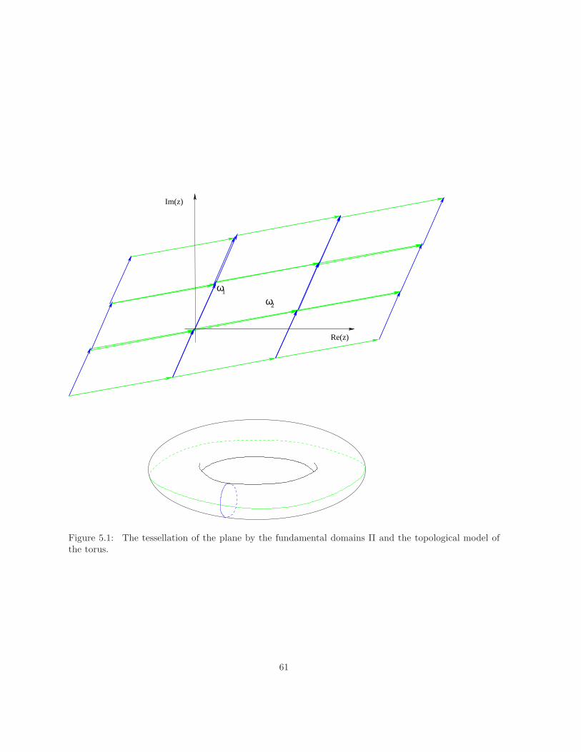
ωω
1
2
Im(z)
Re(z)
Figure 5.1: The tessellation of the plane by the fundamental domains Π and the topological model ofthe torus.
61
and by
Π := z = ω1s1 + ω2s2, s1, s2 ∈ [0, 1) (5.8.11)
the fundamental parallelogram (any point [z] ∈ C/Λ admits a unique representative in the funda-
mental parallelogram).
We will denote by E(ω1, ω2) the complex torus obtained in this way by quotienting C/Λ(ω1, ω2).
A holomorphic/meromorphic function on C/Λ is –similarly to the previous example– a doubly pe-
riodic function
f(z) = f(z + ω1) = f(z + ω2) . (5.8.12)
It is easy to see directly (i.e. without invoking Thm. 5.1.3) that a doubly holomorphic function is constant,
for it is bounded on the parallelogram and –by periodicity– also on the whole complex plane and hence
by Liouville’s theorem is constant. Therefore the only ”interesting” functions are the meromorphic ones,
which are called elliptic functions (by definition doubly periodic meromorphic functions1).
8.1 One-forms
We start by observing that the one form Cdz, C =constant, is well defined since different local coordinates
differ by addition of constants and hence the Jacobian is 1. The one-form dz is clearly then holomorphic
because the local charts are bounded parallelograms in the complex z−plane (this is in contrast with
the case of the Riemann–sphere since dz is not holomorphic, it has a double pole at ∞ (exercise)).
Hence the vector space of holomorphic one-forms is at least one–dimensional: in fact there are no other
holomorphic one-forms, since then it should be of the form
ω = f(z)dz , (5.8.13)
with f(z) doubly periodic and hence constant.
8.2 Elliptic functions
The goal of the following paragraph is to give a precise describition of the field of elliptic functions.
Theorem 5.8.13 The following Weierstrass’ ℘ function is an elliptic function with double poles at
the points of Λ
℘(z) = ℘(z;ω1, ω2) :=1
z2+∑
λ∈Λ′
(1
(z − λ)2− 1
λ2
)(5.8.14)
Λ′ := Λ \ 0. (5.8.15)
1Note that this excludes doubly periodic functions with essential singularities, which are simply referred to as ”doublyperiodic functions”.
62
Proof. We outline the main steps of the proof. We first prove that the series converges to a meromorphic
function with poles at Λ. For any compact K ⊂ C \ Λ we prove uniform convergence. The only concern
arises from the infinite sum over the points of Λ: let R be such that the compact K is contained in the
disk D0(R); since only a finite number of λ’s fall within D0(R) only the part of the sum coming from the
external ones is of concern, since the rest can be easily estimated uniformly (using the δ = dist(K,Λ) > 0)∣∣∣∣∣∣
∑
|λ|>R
(1
(z − λ)2− 1
λ2
)∣∣∣∣∣∣≤∑
|λ|>R
∣∣∣∣2λz − z2
λ2(z − λ)2
∣∣∣∣ ≤∑
|λ|>R
∣∣∣∣2λz − z2
λ2(z − λ)2
∣∣∣∣ ≤∑
|λ|>R
2|λ|R+R2
|λ|2(|λ| −R)2(5.8.16)
This last double series is estimated by an integral of C/r3 over the plane and is therefore convergent.
We also note that ℘(z) is even, ℘(z) = ℘(−z). We now prove that ℘ is doubly periodic; first of all
we note that
℘′(z) = −2∑
λ∈Λ
1
(z − λ)3(5.8.17)
and that it is easy to see that this series as well is uniformly convergent on any compact set in C \ Λ. It
is also easy to see that ℘′(z + λ) = ℘′(z), ∀λ ∈ Λ by shifting the indices of the sum (exercise). Since
the derivative is doubly periodic, the function ℘ must be doubly periodic as well up to additive constant
℘(z + ω1) − ℘(z) = C , ℘(z + ω2) − ℘(z) = D (5.8.18)
Recalling that ℘ is even we evaluate at z = ωi/2 (the half periods)
℘(ω1/2)− ℘(−ω1/2) = 0 ℘(ω2/2)− ℘(−ω2/2) = 0 , (5.8.19)
and hence D = C = 0 and ℘ is doubly periodic. Q.E.D.
We need to write also the Laurent series of ℘ at z = 0
Lemma 5.8.19 The Laurent series expansion of ℘(z) around z = 0 is
℘ =1
z2+ 3z2G2 + 5z4G3 + . . .+ (2k + 1)z2kGk+1 + . . . (5.8.20)
Gj =∑
λ∈Λ′
1
λ2j(5.8.21)
Proof. We have
℘(z) =1
z2+∑
λ
1
λ2
(1
(1 − z
λ
)2 − 1
)=
1
z2+∑
λ∈Λ′
∞∑
k=1
(k + 1)zk
λk+2(5.8.22)
The last triple series is uniformly absolutely convergent for |z| < min(|ω1|, |ω2|) − ǫ and hence we can
interchange the order of the sums obtaining (note that the odd terms cancel because of the symmetry
Λ = −Λ)
℘ =1
z2+ 3z2G4 + 5z4G6 + . . .+ (2k + 1)z2kG2k+2 + . . . (5.8.23)
G2j =∑
λ∈Λ′
1
λ2j=
∑
Z2∋(m,n) 6=(0,0)
1
(mω1 + nω2)2j=
1
ω12j
∑
Z2∋(m,n) 6=(0,0)
1
(m+ nτ)2j(5.8.24)
63
The functions G2j are called Eisenstein’s series and it is easily seen that they are absolutely convergent
(and uniformly in τ = ω2/ω1 for ℑ(τ) > ǫ > 0). Q.E.D.
Theorem 5.8.24 Weierstrass’ function ℘ satisfies the differential equation
(℘′)2 = 4℘3 − g2℘− g3 , g2 := 60G4 , g3 = 140G6 . (5.8.25)
Proof. We take the Laurent expansion of ℘′ and square it
℘′ =−2
z3+ 6zG4 + 20z3G6 + . . . (5.8.26)
(℘′)2 =4
z6− 24
z2G4 − 80G6 + O(z) , (5.8.27)
Therefore we subtract a suitable polynomial in ℘ so as to eliminate the singular part:
(℘′)2 − 4℘3 = −60
z2G4 − 140G6 −O(z) (5.8.28)
(℘′)2 − (4℘4 − g2℘− g3) = O(z). (5.8.29)
Since the LHS is obviously an elliptic function so is the RHS. Moreover the LHS may have poles a priori
only on Λ, but the RHS is telling that it has instead a zero at z = 0 ∈ Λ and hence is holomorphic and
vanishes at one point so it is identically zero. Q.E.D.
The content of Thm. 5.8.24 is that if we set X = ℘(z), Y = ℘(z) we obtain a parametrization of the
following algebraic curve
Y 2 = 4X3 − g2X − g3 . (5.8.30)
According to the terminology of algebraic curves, this is an instance of hyperelliptic curve of genus 1. In
order to prove that ℘ and ℘′ actually parametrize completely the curve (5.8.30) we prove the following
result
Proposition 8.1 Let f(z) be an elliptic function (meromorphic). Let Z := zn and P := pℓ be the
sets of zeroes/poles (both are finite) chosen in the fundamental parallelogram Π and let mn, kℓ be the
multiplicities/orders. Then
1. The number of zeroes (conted with multiplicities) minus the number of poles (counted with their
order) is zero ∑mn =
∑kℓ (5.8.31)
2. The sum of the positions of the zeroes (with multiplicities) minus the sum of the positions of the
poles (with the orders) is a point of Λ
∑
n
mnzn −∑
ℓ
kℓpℓ = λ ∈ Λ (5.8.32)
64
Proof. We will use Corollary 2.7.9. For the path γ we choose the boundary ∂Π and obtain
∮
∂Π
=
∫ ω1
0
+
∫ ω1+ω2
ω1
+
∫ ω2
ω1+ω2
+
∫ 0
ω2
(5.8.33)
where the integrals are supposed to be straight segments (which is mostly irrelevant due to Cauchy’s
theorem). We now integrate the differential f ′(z)f(z) dz (which is elliptic!) on this path and note that -due
to ellipticity- the first integral is minus the third and the second is minus the fourth, e.g. (actually for
any elliptic function g(z)) ∫ ω1
0
g(z)dz =
∫ ω1+ω2
ω2
g(z − ω2)dz (5.8.34)
[If by any chance one of the poles of f ′(z)f(z) falls exactly on the boundary, we translate the fundamental
parallelogram by ǫ to avoid this.]
Therefore we have ∮
∂Π
f ′(z)
f(z)dz = 0 (5.8.35)
and the first assertion follows. For the second we integrate z f ′(z)f(z) dz which is not elliptic, so some care
must be paid
∫ ω1
0
zf ′(z)
f(z)dz −
∫ ω1+ω2
ω2
zf ′(z)
f(z)dz =
∫ ω1
0
(zf ′(z)
f(z)− (z + ω2)
f ′(z + ω2)
f(z + ω2)
)dz = ω2
∫ ω1
0
d(ln(f(z))
∫ ω1+ω2
ω1
zf ′(z)
f(z)dz −
∫ ω2
0
zf ′(z)
f(z)dz =
∫ ω1
0
((z + ω1)
f ′(z + ω1)
f(z + ω1)− z
f ′(z)
f(z)
)dz = ω1
∫ ω2
0
d(ln(f(z))
The integrals in the RHS’s are integer multiples of the periods since -e.g.- the segment [0, ω1] is mapped
to a loop by the elliptic map f(z) and hence the integral just counts the winding number of the loop
w.r.t. zero. Q.E.D.
We thus have
Proposition 8.2 The funcion ℘(z) takes on every value c ∈ C exactly twice (counting with multiplicity)
in each fundamental domain.
Proof. Since ℘ has only one double pole, it must have two zeroes by Prop. 8.1. The same applies to the
elliptic function ℘(z) − c. Q.E.D.
Note that since ℘ is even the two values are taken on at zc and −zc ≡ ω1 + ω2 − zc, i.e. at points
symmetrically placed w.r.t. the center of the fundamental parallelogram Π: at those points ℘′ takes on
opposite values and hence we have proved
Corollary 5.8.35 The functions X = ℘(z) and Y = ℘′(z) give a complete parametrization of the locus
(5.8.30).
65
We finally characterize all meromorphic elliptic functions.
Theorem 5.8.35 Any meromorphic elliptic function f(z) can be uniquely written as
f = R1(X) + Y R2(X) , X = ℘(z) , Y = ℘′(z) (5.8.36)
where R1, R2 are rational functions.
Proof. We split f in its even and odd parts (which are still elliptic),
fe(z) =1
2(f(z) + f(−z)) fo(z) =
1
2(f(z) − f(−z)) . (5.8.37)
Since fo/℘′(z) is even we need only to prove that any even elliptic function can be (uniquely) written as
a rational function of ℘. This is left as exercise. Q.E.D.
Definition 8.3 The algebraic curve (5.8.30) is called a elliptic curve of modulus τ = ω2
ω1.
Coordinate charts and compactification of the algebraic curve
Consider now an arbitrary algebraic curve
L :=
(X,Y ) : Y 2 = 4X3 − g2X − g3
(5.8.38)
where we assume that the roots of P (X) = 4X3−g2X−g3 = 4(X−e1)(X−e2)(X−e3) are distinct (hence
g23 − 27g3
2 6= 0). This subset of C2 is clearly not compact: we perform a one-point compactification
L = L ∪ ∞ (5.8.39)
by adding a formal point at infinity. We need to define the local charts and local coordinates.
1. For a neighborhood of a point (X0, Y0) ∈ L with X0 6= ej we declare that the local coordinate is X
itself (which locally and univocally parametrizes a neighborhood of L near the given point.
2. In a neighborhood of (ej , 0) we declare that the local coordinate is Y (which locally and univocally
parametrizes a neighborhood of L near the given point).
3. A neighborhood of ∞ is in the usual sense: local coordinate is ξ = XY . Introducing η = 1
Y , the
functions ξ, η satisfy (from the same algebraic equation)
η = 4ξ3 − g2ξη2 − g3η
3 (5.8.40)
and the point that we are adding has ξ = 0 = η.
66
Remark 8.1 This definition of coordinate at the ∞ point comes from a ”natural” embedding of L as a subsetof a 2-dimensional complex compact manifold called CP2. It is defined as
CP 2 := C3 \ 0/C
× , (5.8.41)
where the quotient is with respect to the group action of the (Abelian) group C× of nonzero complex numbers,acting on C3 \ 0 by
λ · (z1, z2, z3) := (λz1, λz2, λz3) (5.8.42)
We do not enter in any further detail here.
Exercise 8.3 Prove that the unique (up to scalar multiplication) differential of the first kind on the
elliptic curve of modulus τ can be written as
ω =dX
Y. (5.8.43)
In particular you should prove (check) that the given differential is holomorphic at all points (in particular
at the branchpoints ej and at ∞).
Hence conclude that the coordinate z is given by the elliptic integral
z =
∫dX√
4X3 − g2X − g3(5.8.44)
Exercise 8.4 Prove that the Eisenstein series Gk are all polynomials in G2, G3 with rational coefficients
by following the given steps.
1. From the ODE for ℘ derive the second order ODE
℘′′(z) = 6℘2 − g2 (5.8.45)
2. Match the Laurent series expansions of the two sides (the LHS is linear in the Gk’s, the RHS is
quadratic) and derive a recurrence relation for the Gk’s.
3. Draw the conclusion by induction on the recurrence relations found in the previous step.
There is still a problem that we did not address: indeed so far we have proved that if g2, g3 are given
by the expressions (5.8.25) then ℘ and ℘′ give a parametrization (a.k.a. uniformization) of the locus
of C2
Y 2 = 4X3 − g2X − g3 , (5.8.46)
in terms of the complex torus C/(ω1Z + ω2Z). Suppose that we instead assign two complex numbers
g2, g3 and seek an uniformization for this locus: the natural question is wether there is an elliptic curve
with some modulus τ and hence some periods ω1, ω2 for which the Weierstrass functions ℘, ℘′ yield the
desired uniformization.
Before addressing this in full we make the following remark on an elliptic curve:
67
Proposition 8.3 Let g2, g3 be given by (5.8.25). Then
∆ := g23 − 27g3
2 6= 0 (5.8.47)
Proof. The expression for ∆ is nothing but the discriminant of the polynomial
P (X) = 4X3 − g2X + g3 (5.8.48)
defined as the product of the squares of the differences of the roots. We call the roots of P (X) e1, e2, e3
P (X) = 4(X − e1)(X − e2)(X − e3) . (5.8.49)
We claim that (up to permutation)
e1 = ℘(ω1
2
), e2 = ℘
(ω2
2
), e3 = ℘
(ω3
2
)ω3 := ω1 + ω2 (5.8.50)
Indeed at these points (called the half periods) the function ℘′ is zero by antisymmetry and hence so
is P (X). Since the polynomial is of the third degree, there are no other roots. We have thus
g2 = 4(e1e2 + e2e3 + e3e1) , g3 = 4e1e2e3. (5.8.51)
It is an exercise to see that
(e1 − e2)2(e2 − e3)
2(e1 − e3)2 = ∆ . (5.8.52)
Therefore we must prove that ei 6= ej , i 6= j. Suppose that e1 = e2 (the other cases will be ruled out
similarly). Since ℘−e1 has precisely two zeroes (including multiplicities) and they are symmetric around
the center of Π, this would imply that ω2/2 = −ω1/2 mod Λ, which is not the case. (Note that this
argument also proves that ℘− ej has a double zero since ωj/2 ≡ −ωj/2). Q.E.D.
We should now prove the converse, namely
Theorem 5.8.52 For any two complex numbers g2, g3 such that
g23 − 27g3
2 6= 0 (5.8.53)
there is an elliptic curves with periods ω1, ω2 and modular parameter τ = ω2
ω1∈ ℑ(t) > 0 uniformizing
the algebraic curve
Y 2 = 4X3 − g2X − g3 . (5.8.54)
Proof. The requirement on the discriminant says that the curve is a non-singular hyperelliptic curve of
genus 1 (see Section 11.3). Let us call e1, e2, e3 the distinct roots of P (X) = 4X3 − g2X − g3. Let D the
domain obtained by cutting C along a curve ℓ1 from e1 to e2 and one ℓ2 from e3 to ∞. On this domain
68
Y =√P is single valued (choosing arbitrarily one determination of the square root and analytically
continuing to D) as discussed in Sec. 11.3. We define
Ω1 :=
∮
γ1
dX√P (X)
, Ω2 :=
∮
γ2
dX√P (X)
, (5.8.55)
where γ1 encircles e1, e2 and γ2 encircles e2, e3. They are the periods of the unique Abelian integral of
the first kind
u(X) =
∫ X
X0
dx√P (x)
(5.8.56)
where the path of integration is a curve avoiding the branchpoints. We claim that u(X) defines a local
coordinate in the neighborhood of the compactified elliptic curve; indeed near ej the integrand has an
integrable singularity (inverse square root) and hence u(ej) are well defined. According to the general
theory of hyperelliptic curves (Sec. 11.3) near ej the local coordinate is Y and u(Y ) is holomorphic there
(check!). The only remaining point is ∞: since the integrand is O(X−3/2) also X = ∞ is an integrable
singularity the check of the holomorphicity is left as exercise (note that acccording to the homotopy class
of the contour chosen to approach X = ∞ the resulting values of u(∞) will differ by an integral linear
combination of the periods).
Since u(X) depends on the contour of integration from X0 to X only by addition of mΩ1 + nΩ2,
m,n ∈ Z (see Sec. 11.3), we have (almost) completed the proof if we can show that Ω2
Ω1is not a real
number, so that the map
u : L → C/ZΩ1 + ZΩ2 (5.8.57)
defines a biholomorphism between the algebraic curve and the elliptic curve (in the sense of quotient of
C by the lattice of periods). The fact that ℑ(
Ω2
Ω1
)6= 0 is a particular case of a theorem going under the
name of Riemann theorem (one of the many under the same name!). At this point one should even prove
that Ωi are nonzero2. Consider the simply-connected domain L0 ⊂ L obtained as follows: it is described
as a two–sheeted covering of the domain D0 obtained by cutting C from e1 to e2 and from e2 to e3 and
from e3 to ∞; the two sheets D0,± will be glued only along one segment, for example the one from e3
to ∞ (see Figure 5.2).
We invoke your intuition that this domain is simply connected and hence the function u(X) admits
analytic continuation to a well-defined holomorphic function (the domain so constructed is the so–called
canonical dissection of the compact curve L). If your intuition fails then we can actually prove that
the value of u(X) is the same whether we use for the integration∫ X
X0du the ”direct” (homotopy class of
2Consider the function F (X) = ℑ(P (X)); it splits the X plane into two domains F (X) < 0 and F (X) > 0. Theboundary F (X) = 0 contains the branchpoints ej ’s (since P (ej) = 0) and it is a piecewise smooth curve. On an arc joininge1 to e2 the real part has a definite sign (positive or negative) since otherwise at some other point also ℜ(P (X)) = 0 andwe would have another root of P (X). The abelian integrals on these segments cannot vanish.
69
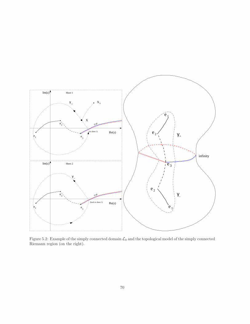
(to sheet 2)
(back to sheet 1)
γ
γ−
+
Re(z)
Im(z)
e
e
e1
2
3
Cut
Sheet 2
Re(z)
Im(z)
e
e
e1
2
3
Cut
Sheet 1
X
X
0
infinity
e3
γ−
γ
e
+
1
e2
e2
e1
Figure 5.2: Example of the simply connected domain L0 and the topological model of the simply connectedRiemann region (on the right).
70
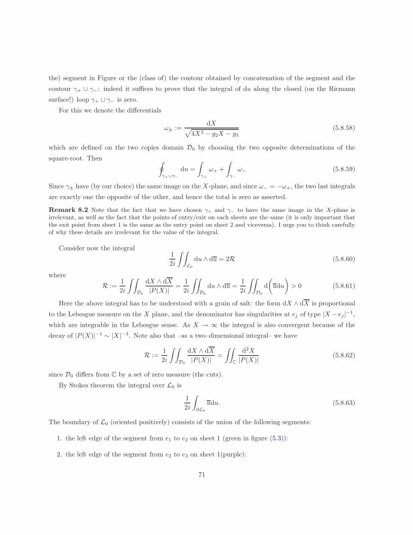
the) segment in Figure or the (class of) the contour obtained by concatenation of the segment and the
contour γ+ ∪ γ−: indeed it suffices to prove that the integral of du along the closed (on the Riemann
surface!) loop γ+ ∪ γ− is zero.
For this we denote the differentials
ω± :=dX√
4X3 − g2X − g3(5.8.58)
which are defined on the two copies domain D0 by choosing the two opposite determinations of the
square-root. Then ∮
γ+∪γ−
du =
∫
γ+
ω+ +
∫
γ−
ω− (5.8.59)
Since γ± have (by our choice) the same image on the X-plane, and since ω− = −ω+, the two last integrals
are exactly one the opposite of the other, and hence the total is zero as asserted.
Remark 8.2 Note that the fact that we have chosen γ+ and γ− to have the same image in the X-plane isirrelevant, as well as the fact that the points of entry/exit on each sheets are the same (it is only important thatthe exit point from sheet 1 is the same as the entry point on sheet 2 and viceversa). I urge you to think carefullyof why these details are irrelevant for the value of the integral.
Consider now the integral1
2i
∫ ∫
L0
du ∧ du = 2R (5.8.60)
where
R :=1
2i
∫ ∫
D0
dX ∧ dX
|P (X)| =1
2i
∫∫
D0
du ∧ du =1
2i
∫∫
D0
d
(udu
)> 0 (5.8.61)
Here the above integral has to be understood with a grain of salt: the form dX ∧ dX is proportional
to the Lebesgue measure on the X plane, and the denominator has singularities at ej of type |X − ej|−1,
which are integrable in the Lebesgue sense. As X → ∞ the integral is also convergent because of the
decay of |P (X)|−1 ∼ |X |−3. Note also that –as a two–dimensional integral– we have
R :=1
2i
∫ ∫
D0
dX ∧ dX
|P (X)| =
∫∫
C
d2X
|P (X)| (5.8.62)
since D0 differs from C by a set of zero measure (the cuts).
By Stokes theorem the integral over L0 is
1
2i
∫
∂L0
udu. (5.8.63)
The boundary of L0 (oriented positively) consists of the union of the following segments:
1. the left edge of the segment from e1 to e2 on sheet 1 (green in figure (5.3)):
2. the left edge of the segment from e2 to e3 on sheet 1(purple):
71
Sheet 1
Re(z)
Im(z)
e
e
e1
2
3
Cut
Re(z)
Im(z)
e
e
e1
2
3
Cut
Sheet 2
X X −+
Figure 5.3: The boundary of the simply connected Riemann region L0 (the two edges of each segmentare drawn separate only for didactical purposes).
3. the left edge of the segment from e3 to e2 on sheet 2 (purple):
4. the left edge of the segment from e2 to e1 on sheet 2 (brown):
5. the left edge of the segment from e1 to e2 on sheet 2 (brown):
6. the left edge of the segment from e2 to e3 on sheet 2(cyan):
7. the left edge of the segment from e3 to e2 on sheet 1 (cyan):
8. the left edge of the segment from e2 to e1 on sheet 1 (green).
Note that two segments of the same color close to a loop on our original Riemann surface L; we call the
green one the a-cycle and the puple one the b-cycle. For reasons that should become clear later on we
call the brown one a(−) and the cyan one b(−).
Next we note that the value of u(X) on corresponding points of the green and brown contours differ
by the period on the cyan (b) cycle: indeed if X+ is a point on the ”lower” edge of the green contour and
X− is the same point on the lower edge of the brown contour, then the value of u are related by (refer to
Fig. 5.3).
u(X−) = u(X+) −∮
γ
du , (5.8.64)
where γ is a loop winding around e2 and e3 clockwise, hence homotopic to the opposite of the b-cycle.
Therefore we have
u(X+) − u(X−) = Ω2 =:
∮
b
dX
Y(5.8.65)
72
Similarly for points Y± on the purple and cyan contours
u(Y+) − u(Y−) = −Ω1 =: −∮
a
dX
Y. (5.8.66)
Note also that∮
a du = −∮a(−) du (and similarly for the b-cycles) due to the fact that the analytic
continuation of the square root changes sign. More explicitly
∮
a
du =
∫ e1
e2
ω+ +
∫ e2
e1
ω+ = 2
∫ e2
e1
ω+ (5.8.67)
∮
a(−)
du =
∫ e1
e2
ω− +
∫ e2
e1
ω− = 2
∫ e2
e1
ω− = −∮
a
du . (5.8.68)
This explains the notation: a and a(−) are in fact the same contour (homologically) run in opposite
direction (ditto for b and b(−)).
We can now proceed with the computation of the integral (5.8.60):
∫
∂L0
udu =
∫
a
udu+
∫
b
udu+
∫
a(−)
udu+
∫
b(−)
udu = (5.8.69)
=
∫
a
(u(X+) − u(X−))du+
∫
b
(u(Y+) − u(Y−))du = (5.8.70)
= Ω2
∮
a
du+ Ω1
∮
b
du = (5.8.71)
= Ω2Ω1 − Ω2Ω1 (5.8.72)
so that we obtain
0 <1
2i
∫ ∫
L0
du ∧ du =1
2i
(Ω2Ω1 − Ω1Ω2
)= ℑ(Ω2Ω1) = ℑ
(|Ω2|2
Ω1
Ω2
)(5.8.73)
which proves that the imaginary part of the ratio τ = Ω1/Ω2 must be nonzero and actually positive (the
sign is due to the definition of Ωi and the relative orientations of the a and b cycles).
We have therefore proved that our curve L is biholomorphically equivalent to the complex torus
E(Ω1,Ω2). If we consider the Abelian integral u(X) and invert it, we obtain an elliptic function which
we identify with the ℘-function (up to a shift) since ℘ and ℘′ satisfy the same algebraic equation as X,Y .
Q.E.D.
We conclude this section with a few remarks on the choices of the cycles a and b made in the proof
of Thm. 5.8.52. One can in fact choose different ways of ”canonically” dissecting the elliptic curve but
the dissection must be such that the resulting domain is connected and simply-connected. The different
choices depend on where we decide to put the various cuts and glueing; for example we could have decided
that the cuts be done from e1 to e3 and e3 to e2 and e2 to ∞ instead of our choice. The resulting new a
73
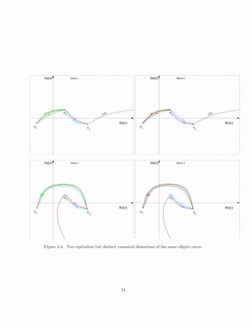
Re(z)
Im(z)
e
e
e1
2
3
Cut
Sheet 1
Re(z)
Im(z)
e
e
e1
2
3
Cut
Sheet 2
Re(z)
Im(z)
e
e
e1
2
3
Sheet 2
Re(z)
Im(z)
e
e
e1
2
3
Sheet 1
Figure 5.4: Two equivalent but distinct canonical dissections of the same elliptic curve.
74
and b cycles would then differ from the previous ones. Looking at Fig. 5.4 we see that the new a-cycle
(green) is homotopic to the concatenation of the previous green and purple. It follows that
Ω1 =
∮
ea
du =
∮
a
du+
∮
b
du = Ω1 + Ω2 . (5.8.74)
Once a dissection has been made the identification of a and b cycles follows in such a way that the
intersection number between a and b cycle is +1.
8.3 Automorphisms and equivalence of complex tori
We now study the equivalence classes of elliptic curves (modulo the relation of biholomorphic equivalence):
since we have proved that any elliptic curve is equivalent to a complex torus, the study is tantamount
classifying complex tori. In particular we would like to ”parametrize” the collection of all classes of
inequivalent complex tori.
By the very definition any complex torus E(ω1, ω2) is uniquely defined by its periods ω1 and ω2:
however we cannot exclude that there is another complex torus E(η1, η2) with different periods but
biholomorphically equivalent to the first.
Since all the information is encoded in the lattices of the periods, the question to ask is; given two
lattices Λ, Λ of periods, find under what conditions there is a holomorphic and invertible map f : C → C
such that f(Λ) = Λ and
f(z + ω1) = f(z) + aη1 + bη2
f(z + ω2) = f(z) + cη2 + dη2 , a, b, c, d ∈ Z
f−1(w + η1) = f−1(w) + a′ω1 + b′ω2
f−1(w + η2) = f−1(w) + c′ω2 + d′ω2 , a′, b′, c′, d′ ∈ Z . (5.8.75)
We immediately observe that the only candidates for such function f are linear (or affine maps)
f(z) = Az +B , (5.8.76)
for, from the requirements, f ′(z) is elliptic (w.r.t. the first lattice) and bounded and hence constant.
The constant B can be reabsorbed in a suitable shift of z and hence we are left only with f = Az
(and A 6= 0 for otherwise the map is not invertible). The next observation is that we can certainly
substitute a complex torus E(ω1, ω2 a biholomorphically equivalent one E(1, τ), with τ = ω2
ω1by using
A = 1ω1
. Therefore without loss of generality the conditions (5.8.75) can be posed for ω1 = 1, ω2 = τ
and η1 = 1 , η2 = τ ′ with both τ, τ ′ ∈ ℑ(w) > 0. Then
75
Lemma 5.8.76 The matrices
(a bc d
)and
(a′ b′
c′ d′
)which enter (5.8.75) must be inverse of each other
and hence have determinant = ±1. If in addition the periods are ordered so that the modular parameters
have both positive imaginary parts then(a bc d
)∈ SL2(Z) . (5.8.77)
Exercise 8.5 Prove the Lemma.
Proposition 8.4 Two complex tori E(1, τ) and E(1, τ ′), with τ, τ ′ ∈ ℑ(w) > 0 are biholomorphically
equivalent iff there is a matrix
(a bc d
)∈ SL2(Z) such that
τ ′ = g · τ :=aτ + b
cτ + d(5.8.78)
Exercise 8.6 Prove that the group Γ = SL2(Z) acts on ℑ(τ) > 0, namely that
τ ′ = g · τ :=aτ + b
cτ + d(5.8.79)
has ℑ(τ ′) > 0 and that this is a group action.
Exercise 8.7 Prove the Proposition and find also the constant A appearing in the isomorphism.
9 Modular group and modular forms
The group SL2(Z) is called the (full) modular group. The action of Γ on H+ := ℑ(τ) > 0 has a
kernel ±1. The quotient group is called PSL2(Z) and the action is then faithful; it is however more
practical to study directly the full modular group.
It can be proved that any g ∈ Γ can be obtained by composing the following two generators
T : T · τ = τ + 1 , T =
(1 10 1
)(5.9.1)
S : S · τ = −1
τ, S =
(0 −11 0
). (5.9.2)
The fundamental domain for the action namely a set such that any τ ∈ H+ := ℑ(τ) > 0 has a
unique τ ′ = g · τ in such set, can be chosen as
D0 :=
τ : |τ | > 1, ℜ(τ) ∈ [−1
2,1
2), ℑ(τ) > 0
∪|τ | = 1, ℑ(τ) > 0,ℜ(τ) ∈ [−1
2, 0]
(5.9.3)
Exercise 9.1 Prove that ∀τ ∈ H+ there is an element g ∈ SL2(Z) such that gτ ∈ D0. (Use an appro-
priate sequence of T and S transformations to place τ in the fundamental domain. Draw pictures!).
76
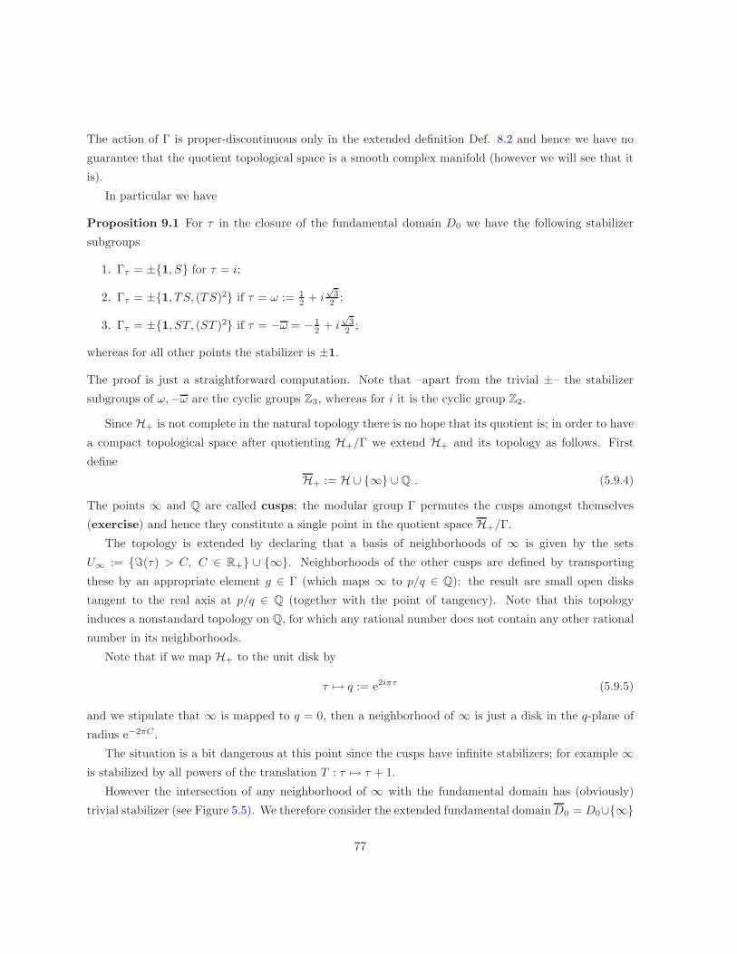
The action of Γ is proper-discontinuous only in the extended definition Def. 8.2 and hence we have no
guarantee that the quotient topological space is a smooth complex manifold (however we will see that it
is).
In particular we have
Proposition 9.1 For τ in the closure of the fundamental domain D0 we have the following stabilizer
subgroups
1. Γτ = ±1, S for τ = i;
2. Γτ = ±1, TS, (TS)2 if τ = ω := 12 + i
√3
2 ;
3. Γτ = ±1, ST, (ST )2 if τ = −ω = − 12 + i
√3
2 ;
whereas for all other points the stabilizer is ±1.
The proof is just a straightforward computation. Note that –apart from the trivial ±– the stabilizer
subgroups of ω,−ω are the cyclic groups Z3, whereas for i it is the cyclic group Z2.
Since H+ is not complete in the natural topology there is no hope that its quotient is; in order to have
a compact topological space after quotienting H+/Γ we extend H+ and its topology as follows. First
define
H+ := H ∪ ∞ ∪ Q . (5.9.4)
The points ∞ and Q are called cusps; the modular group Γ permutes the cusps amongst themselves
(exercise) and hence they constitute a single point in the quotient space H+/Γ.
The topology is extended by declaring that a basis of neighborhoods of ∞ is given by the sets
U∞ := ℑ(τ) > C, C ∈ R+ ∪ ∞. Neighborhoods of the other cusps are defined by transporting
these by an appropriate element g ∈ Γ (which maps ∞ to p/q ∈ Q): the result are small open disks
tangent to the real axis at p/q ∈ Q (together with the point of tangency). Note that this topology
induces a nonstandard topology on Q, for which any rational number does not contain any other rational
number in its neighborhoods.
Note that if we map H+ to the unit disk by
τ 7→ q := e2iπτ (5.9.5)
and we stipulate that ∞ is mapped to q = 0, then a neighborhood of ∞ is just a disk in the q-plane of
radius e−2πC .
The situation is a bit dangerous at this point since the cusps have infinite stabilizers; for example ∞is stabilized by all powers of the translation T : τ 7→ τ + 1.
However the intersection of any neighborhood of ∞ with the fundamental domain has (obviously)
trivial stabilizer (see Figure 5.5). We therefore consider the extended fundamental domainD0 = D0∪∞
77
i
1+i 32
=ω
0 1/21/3 12/3
Figure 5.5: The fundamental domain (cyan) with a neighborhood of ∞; also marked are other twofundamental domains with corresponding neighborhoods of the cusp.
78
where ∞ has been added to the standard fundamental domain and a basis of neighborhoods is the
intersection of the previously defined ones with this domain.
The topology defined on D0 near ∞ is precisely such that the map τ 7→ q = e2iπτ is continuous at the
cusp i∞; more than that, it has defined a local coordinate which we use in order to define the analytic
structure. We will say that a holomorphic/meromorphic periodic function f(τ) = f(Tτ) = f(τ +1) has
a pole/zero of order/multiplicity m if
f(e2iπτ ) := f(τ) (5.9.6)
has a Laurent-series expansion of the form
f(q) =∞∑
n=±m
cnqm . (5.9.7)
Exercise 9.2 Show that topologically H+/Γ is homeomorphic to the set D0/ ∼ where the relation ∼identifies
τ = −1
2+ ir ∼ 1
2+ ir, (5.9.8)
τ = eiθ ∼ −e−iθ for θ ∈ [π/3, π/2) (5.9.9)
So far we have proved that the equivalence classes of elliptic curves/complex tori are in one-to-one
correspondence with the orbits of H+ under the action of Γ = PSL2(Z)3. In order to define a complex
structure on this set we seek a function J(τ) which has the following properties
1. J : H+ → C is holomorphic in H+
2. J(τ) takes on the same values on points of the same orbit, namely
J
(aτ + b
cτ + d
)= J(τ) ∀τ ∈ H+ , ∀
(a bc d
)∈ SL2(Z). (5.9.10)
In such a way we may think of J : H+/Γ → C so that J([τ ]) = J(τ).
3. For any two disjoint orbits the values of J are different i.e. J separates the points of H+/Γ.
If such a function exists (and in fact it does) then we define the complex structure on H+/Γ by decreeing
that J([τ ]) is a complex coordinate: note that this implies that we can cover the whole space with only
one chart. Before constructing J(τ) we make an important digression in the following section.
3The orbits of a group acting on a manifold are the equivalence classes of points which are connected by a trasformationof the said group.
79
9.1 Modular functions and forms
Definition 9.1 A meromorphic function f(τ) defined on the upper half-plane H+ is called a mero-
mophic modular function of weight k (k an integer) if it satisfies the relation
f(gτ) = (cτ + d)kf(τ) , g =
(a bc d
)∈ SL2(Z) , (5.9.11)
and it is meromorphic at infinity in the sense that its Fourier series representation has at most a finite
number of negative frequencies
f(τ) =∑
n>>−∞cnq
n , q = e2iπτ . (5.9.12)
If f(τ) is holomorphic at all points including infinity, we then call it a modular form of weight k and
the set of modular forms of weight k will be denoted by Mk = Mk(Γ). A modular form is called a cusp
form if it vanishes at the cusp i∞ and their set is denoted by Ek = Ek(Γ).
In the definition we have used the full modular group Γ = SL2(Z) but one could give a similar definition
for subgroups Γ′ of Γ; in this case one should specify ”modular form for Γ′”.
In the definition of modular function we have in particular for T and S that
f(τ + 1) = f(τ) , T =
(1 10 1
)(5.9.13)
f(−1/τ) = (−τ)kf(τ) . , S =
(0 −11 0
)(5.9.14)
Remark 9.1 Since T, S generate SL2(Z) in order to verify that a function is modular of weight k it is sufficient(and usually much easier) to verify the two relations (5.9.14): the invariance under T in particular implies thatmodular functions are periodic functions of period 1 and hence can be expanded in Fourier series of q = e2iπτ . Itis also easy to see (using −1 ∈ SL2(Z) in eqs. (5.9.14)) that there are no (nontrivial) modular functions of oddweight, and hence we assume from now on that the weight is an even number.
Remark 9.2 Sincedgτ
dτ= (cτ + d)−2 (5.9.15)
we can rephrase Def. 9.1 by saying that the tensor ω := f(τ )(dτ )k2 is invariant under the modular group.
It is obvious that the set of modular functions/forms/cusp forms of a fixed weight is a vector space.
Moreover if we multply/divide two modular functions f, h of weights k, j we obtain another modular
function of weight k+ j or k− j, hence the set of modular functions of all weights is a field. In particular
we have the subfield of modular functions of weight zero.
We have previously introduced the Eisenstein series in the course of the proof of Lemma 5.8.19 as
functions on the space of lattices. Since they are homogeneous in the periods we can always set one of
80
the periods to 1 and the other to τ ∈ H+. We now reintroduce the definition of the Eisenstein series
which is more appropriate in the context of modular functions as follows
G2k(τ) :=
′∑
n,m
1
(mτ + n)2k, k ≥ 2 , (5.9.16)
where the prime indicates that the term m = 0 = n is omitted. We have already remarked that it is easy
to show that the double series are absolutely convergent and uniformly over any compact set of H+.
By elementary manipulation of series it follows that
G2k(τ + 1) = G2k(τ) (5.9.17)
G2k
(−1
τ
)= τ2kG2k(τ) , (5.9.18)
and hence they are modular functions. Moreover they have a well-defined value at τ → i∞
limτ→i∞
G2k(τ) = limτ→i∞
′∑
n,m
1
(mτ + n)2k=∑
n6=0
1
n2k= 2ζ(2k) (5.9.19)
In the literature it is often found a normalized Eisenstein series, where the normalization is such that
they take value 1 at ∞E2k(τ) :=
1
2ζ(2k)G2k(τ) . (5.9.20)
They have the property (useful in the applications to number theory) that the coefficients in the q
expansion are rational
E2k(τ) = 1 − 2k
Bk
∞∑
n=1
σk−1(n)qn (5.9.21)
σk−1(n) :=∑
d|ndk−1 (5.9.22)
x
ex − 1=
∞∑
k=0
Bkxk
k!, Bk = Bernoulli numbers. (5.9.23)
Recall that in Weierstrass uniformization we have the functions g2, g3 which are multiples of G4, G6; in
particular a computation shows
Y 2 = 4X3 − g2X − g3 (5.9.24)
g2 = 60G4 =4
3π4E4 , (5.9.25)
g3 = 140G6 =8
27π6E6 . (5.9.26)
The discriminant of the elliptic curve becomes
∆(τ) = g23 − 27g3
2 =(2π)12
1728
(E4
3 − E62
)(5.9.27)
81
which shows, –since E4, E6 are normalized at τ = i∞– that ∆ is a cusp form of weight 12. Summarizing
we have shown that
Proposition 9.2 The (normalized) Eisenstein series are modular forms G2k ∈M2k and the discriminant
∆ is a cusp form ∆ ∈ E12(Γ).
Poles and residues of modular functions
We first prove
Lemma 5.9.27 Let f(τ) a modular function of weight k and γ be a contour in H+ avoiding its poles
and zeroes: let g ∈ SL2(Z), then
∫
γ
f ′(τ)dτ
f(τ)−∫
gγ
f ′(τ)dτ
f(τ)= −k
∫
γ
dτ
τ + d/c(5.9.28)
Proof. Differentiating the identity
f(gτ) = (cτ + d)kf(τ) (5.9.29)
we obtain
f ′(gτ)(cτ + d)−2 = kc(cτ + d)k−1f(τ) + (cτ + d)kf ′(τ) (5.9.30)
f ′(gτ)
f(gτ)dgτ =
f ′(τ)dτ
f(τ)+ k
1
τ + d/c(5.9.31)
so that the LHS of the lemma gives
∫
γ
f ′(τ)dτ
f(τ)− f ′(gτ)
f(gτ)dgτ = −k
∫
γ
dτ
τ + d/c(5.9.32)
The lemma is proved. Q.E.D.
Proposition 9.3 Let f(τ) be a nontrivial modular function of weight k for SL2(Z). let vp(f) denote
the order of the zero (or minus the order of the pole) for p ∈ H+. Let v∞(f) denote the index of the first
nonvanishing term in the q-expansion of f at ∞ (i.e. (minus) the order of the zero/pole at infinity), then
v∞(f) +1
2vi(f) +
1
3vω(f) +
∑
i,ω 6=p∈H+/Γ
vp(f) =k
12(5.9.33)
Proof. We first apply the residue theorem to count poles/zeroes inside the fundamental domain; it could
happen that some (e.g. P,Q in Fig. 5.6) fall exactly on the boundary. In this case some care must be
paid so as to avoid counting the other images of the same points that fall also on the boundary (this is
the reason of the small bumps in the contour).
82
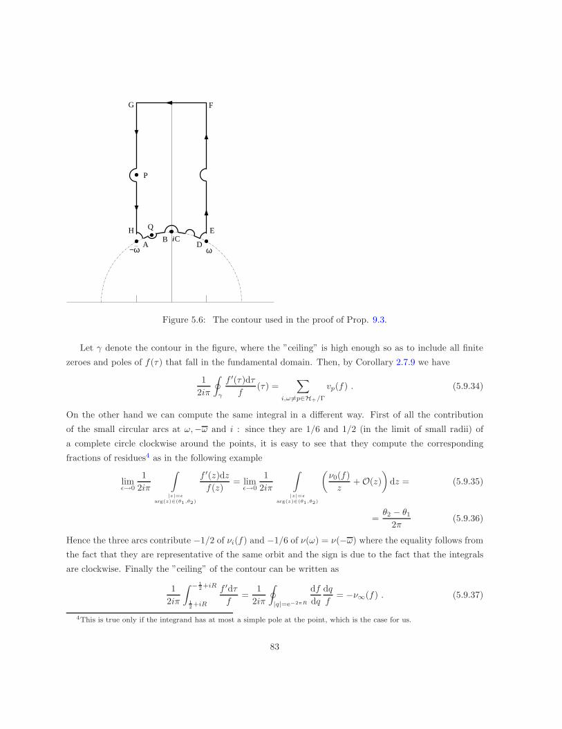
i
P
Q
−ω ω
H
A
EB C
D
FG
Figure 5.6: The contour used in the proof of Prop. 9.3.
Let γ denote the contour in the figure, where the ”ceiling” is high enough so as to include all finite
zeroes and poles of f(τ) that fall in the fundamental domain. Then, by Corollary 2.7.9 we have
1
2iπ
∮
γ
f ′(τ)dτ
f(τ) =
∑
i,ω 6=p∈H+/Γ
vp(f) . (5.9.34)
On the other hand we can compute the same integral in a different way. First of all the contribution
of the small circular arcs at ω,−ω and i : since they are 1/6 and 1/2 (in the limit of small radii) of
a complete circle clockwise around the points, it is easy to see that they compute the corresponding
fractions of residues4 as in the following example
limǫ→0
1
2iπ
∫
|z|=ǫ
arg(z)∈(θ1,θ2)
f ′(z)dz
f(z)= lim
ǫ→0
1
2iπ
∫
|z|=ǫ
arg(z)∈(θ1,θ2)
(ν0(f)
z+ O(z)
)dz = (5.9.35)
=θ2 − θ1
2π(5.9.36)
Hence the three arcs contribute −1/2 of νi(f) and −1/6 of ν(ω) = ν(−ω) where the equality follows from
the fact that they are representative of the same orbit and the sign is due to the fact that the integrals
are clockwise. Finally the ”ceiling” of the contour can be written as
1
2iπ
∫ − 12+iR
12 +iR
f ′dτ
f=
1
2iπ
∮
|q|=e−2πR
df
dq
dq
f= −ν∞(f) . (5.9.37)
4This is true only if the integrand has at most a simple pole at the point, which is the case for us.
83
The two arcs on the unit circle AB and CD are interchanged by S, whereas GH and FE by T ; however
the two integrals on GH and FE cancel each other because of the opposite orientation and the fact that
the differential f ′dτ/f is invariant under T . Therefore it only remains to compute the integrals along
AB and CD. Noting that S · (AB) = DC (i.e. S : τ 7→ − 1τ inverts the orientation) we have
1
2iπ
∫
AB
f ′(τ)dτ
f(τ)+
1
2iπ
∫
CD
f ′(τ)dτ
f(τ)=
1
2iπ
∫
AB
f ′(τ)dτ
f(τ)− 1
2iπ
∫
S·(AB)
f ′(τ)dτ
f(τ)= (5.9.38)
= −k 1
2iπ
∫
AB
dτ
τ→ k
12(5.9.39)
in the limit of small radii of the arcs HA, BC and DE. Therefore we have proved
1
2iπ
∮
γ
f ′(τ)dτ
f(τ)= −v∞(f) − 1
2vi(f) − 1
3vω(f) +
k
12(5.9.40)
and the proof of the proposition follows by rearranging the terms. Q.E.D.
We also have
Proposition 9.4 The modular forms of all weights form a ring with a gradation induced by the weight
M(Γ) =⊕
k∈Z
Mk(Γ) . (5.9.41)
The subspaces of modular forms of fixed weight have the following structure:
1. M0(SL2(Z)) = C (i.e. the only modular forms of weight zero are constants).
2. Mk(SL2(Z)) = 0 if k is negative or odd or k = 2.
3. Mk(SL2(Z)) = CEk (i.e. one-dimensional and generated by an Eisenstein series) for k =
4, 6, 8, 10, 14.
4. S12(SL2(Z)) = C∆.
5. Sk(SL2(Z)) = 0 for k < 12 and k = 14, and for k ≥ 16 we have Sk(SL2(Z)) = ∆Mk−12(SL2(Z)).
6. Mk(SL2(Z)) = Sk(SL2(Z)) ⊕ CEk for k > 12 .
Proof. The fact that modular forms form a graded ring is obvious. For the rest the idea is to use
Prop. 9.3 and the fact that a modular form (by definition) has no poles and hence the RHS of (5.9.33)
is nonnegative.
(1,2,3) If k = 0 in (5.9.33) then there are no zeroes; if f(τ) is in M0 then so is f(τ)− c which has at
least one zero if f is nonconstant. We readily get a contradiction.
If k = 2 in (5.9.33) there is no way of getting 16 also nin the RHS so there are no such modular forms.
If k = 4 we must have vω(f) = 1; since E4 is one such modular form, then E4 has only a simple zero at
84
ω. Then f/E4 is a modular form of weight 0 and hence constant, so any modular form of weight 4 is
proportional to E4. Similarly for E6 (with a simple zero at i), E8 (double zero at ω), E10 (simple zero
at i and ω), E14 (simple zero at i and double zero at ω).
(4) For the case k = 12 we have ∆ (cusp form) and E12, so the dimension of M12 is at least 2; note
also that ∆ has only one zero at infinity. Let f ∈M12; if f(∞) = 0 then f is proportional to ∆ (because
f/∆ is a modular form of weight 0): if f(∞) = c then f − cE12 is proportional to ∆. Hence M12 is
exactly 2-dimensional.
(5) By definition of cusp forms, they must have v∞ > 0 and hence there are none for k < 12. For
k = 12 we have already seen that they are spanned by ∆. If f ∈ Sk then it has a (at least simple) zero
at ∞ and hence f/∆ is a modular form in Mk−12.
(6) If f ∈Mk then either it is a cusp form or f(τ) − f(∞)Ek(τ) is a cusp form. Q.E.D¿
Theorem 5.9.41 (Ring of modular forms) The ring of modular forms is a free graded polynomial
ring in E4, E6
M(Γ) =⊕
k∈N
k 6=2
Mk(Γ) = C[E4, E6] (5.9.42)
Proof. We need to prove that any modular form can be written as a polynomial in E4, E6. This is done
by induction on k. There is nothing to prove for k = 0, 4, 6, 12 (recall that ∆ = (2π)12
1728
(E4
3 − E62
)).
Moreover since Mk = ∆Mk−12 ⊕ CEk we need to express Ek as polynomials of E4, E6.
For k = 8 clearly E8−E42 is a cusp form of weight 8 and hence vanishes (by the previous proposition).
For k = 10 we use E10 − E4E6, for k = 14 we use E14 − E42E6.
For k > 14, in view of the decomposition Mk = ∆Mk−12⊕CEk and proceeding by induction, we need
only to express Ek as a polynomial in E4, E6; to this end note that the diophantine equation
4a+ 6b = k (5.9.43)
admits solution for all even k ≥ 10; if k mod 6 = 0we just take b = k/6; if k mod 6 = 2 we take
b = (k − 8)/6 and a = 2; if k mod 6 = 4 we take b = (k − 4)/2 and a = 1. Hence Ek − E4aE6
b is a cusp
form of weight k and hence also a polynomial in E4, E6. Q.E.D.
Theorem 5.9.43 The function
J(τ) =g2
3(ω1, ω2)
g23 − 27g32=
E43
E43 − E6
2 . (5.9.44)
is SL2(Z)–invariant and takes on each complex value c ∈ C exactly once in the fundamental domain D0
and hence gives a bijection of H+/Γ with the Riemann sphere C.
Remark 9.3 For applications to number theory the J function is normalized differently as j = 1728J .
85
Proof Clearly J − c for c ∈ C is a modular function of weight zero, hence invariant under SL2(Z). Since
it has a simple pole at ∞ it must have either (depending on c) a double zero at i, a triple zero at ω or a
simple zero at some other point of D0. This proves that it takes any value exactly once and hence gives
a bijection with C (and with C if we throw in τ = i∞). Q.E.D.
Remark 9.4 More precisely, since E4(ω) = 0 (see proof. of Prop. 9.4) J has a triple zero at ω. Moreover
E43
E43 − E6
2 = 1 +E6
2
E43 − E6
2 (5.9.45)
and since we have discussed that E6(i) = 0 then J(τ ) − 1 has a double zero at τ = i. In other words J(ω) =0, J(i) = 1 (and clearly J(∞) = ∞).
We can finally put together the theory of the moduli space of complex tori=elliptic curves with the
just developed theory of modular functions by saying that the moduli space of elliptic curves can be given
a structure of smooth compact complex manifold equivalent to the Riemann sphere.
The theory of moduli for other Riemann surfaces is much more complicated and invariably leads to
objects that are not smooth manifolds but have some sort of singularities.
10 Classification of complex one-dimensional manifolds
Exercise 10.1 Prove that C and the unit disk D0(1) are not biholomorphically equivalent. [Hint: use
Liouville’s theorem]
More generally we have
Theorem 5.10.0 (Classification of simply connected curves) Let M be a one-dimensional com-
plex manifold, connected and simply connected. Then it is biholomorphically equivalent to one of the
following
1. The Riemann–Sphere C (see later)
2. The complex plane C
3. The unit disk D0(1) := z : |z| < 1
The classification of non simply–connected one dimensional complex manifolds is reduced to the study
of proper-discontinuous group actions on simply connected manifolds. Indeed we have seen that for any
non simply connected manifold M its universal covering M is acted upon properly-discontinously by the
deck transformations. It can be proved for instance that if π1(M) = Z × Z then it is an elliptic curve of
the kind seen before (for some τ).
86
11 Algebraic functions and algebraic curves
Definition 11.1 A function f(z) defined on a domain D is called algebraic if there exists a polynomial
function P (w, z) such that
P (f(z), z) ≡ 0, z ∈ D. (5.11.1)
The locus
C := (w, z) ∈ C2 : P (w, z) = 0 (5.11.2)
is called an algebraic curve.
Sometimes it is useful to consider a rational function R(X,Y ) instead of a polynomial and the defi-
nition requires a certain specification so as to ”avoid” the zeroes of the denominator.
The second remark is that if P (f(z), z) ≡ 0 in D then so must be for any analytic continuation of
f along any path: indeed if f is the analytic continuation of f then the analytic continuation of P (f(z), z)
is P (f(z), z) and since it is the continuation of the zero function it must be identically zero.
We now prove that a polynomial equation P (w, z) = 0 of degree n in w defines locally n (germs) of
analytic functions. More precisely
Proposition 11.1 Given the algebraic equation P (w, z) = 0 with
P (w, z) = An(z)wn + . . .+A0(z) , An(z) 6≡ 0 , (5.11.3)
and a point (w0, z0) ∈ C2 such that ∂wP
∣∣∣∣(w0,z0)
6= 0 then there is a germ of analytic function f(z) =
w0 +∑
n≥1 cn(z − z0)n which satisfies the functional equation.
Sketch of proof. We regard the function P (w, z) : C2 → C as a C∞ function P : R4 → R2. Then
the condition Pw 6= 0 at (w0, z0) guarantees that the rank of the Jacobian of the function P : R4 → R2
is maximal and can be solved locally for ℜ(w),ℑ(w) yielding differentiable (actually infinitely differen-
tiable) functions of ℜ(z),ℑ(z). Then one has to check that these functions satisfy also Cauchy–Riemann
equations. Q.E.D.
From now on we assume (to avoid trivial occurrences) that P (w, z) is irreducible namely (def) cannot
be written as the product of two non-constant polynomials. For simplicity in the discussions below we
may also require that the discriminant of P (w, z) (viewed as a polynomial in w with parameter z) is
not the identically zero function of z. We recall the definition of the discriminant
Definition 11.2 Given a (monic) polynomal P (X) = aNXN + . . . of degree N in the indeterminate X,
and X1, . . . , XN its roots (possibly repeated) the discriminant is the following expression
∆ := aN2N−1
∏
i<j
(Xi −Xj)2 . (5.11.4)
In particular (by definition) the discriminant is zero iff the polynomial has repeated roots.
87
It can be proved that (example with N = 4)
∆(P ) = det
a4 a3 a2 a1 a0 0 00 a4 a3 a2 a1 a0 00 0 a4 a3 a2 a1 a0
a1 2a2 3a3 4a4 0 0 00 a1 2a2 3a3 4a4 0 00 0 a1 2a2 3a3 4a4 00 0 0 a1 2a2 3a3 4a4
(5.11.5)
from which it is clear that although the definition involves the roots of the polynomial, it is actually a
polynomial of the coefficients aj . So the discriminant of P (w, z) in (5.11.3) is a polynomial in Aj(z) and
hence a polynomial in z.
Suppose now P (w, z) is irreducible and z0 is a point where An(z)∆(w)(P ) is nonzero (and hence
nonzero in a neighborhood U0 of z0. As a polynomial of w depending parametrically on z, P (•, z) = 0
has precisely n = degw P distinct roots wk(z); furthermore we have
Pw(wk(z), z) 6= 0 (5.11.6)
since the roots are distinct (exercise). Then Prop. 11.1 guarantees that each wk(z) is analytic in U0
and hence we have defined n analytic elements (and germs of analytic functions).
To simplify the discussion we assume from now on that the leading coefficient is a constant (and hence
we can assume it to be unity).
P (w, z) = wn + a1(z)wn−1 + . . . . (5.11.7)
It should be clear that this procedure as described fails in a neighborhood of a point z0 such that
An(z)∆(z) = 0. We denote by B := zn the finite set of these points (called ramification points).
Consider a neighborhood U0 of a non-ramification point as earlier and f(z) = w1(z) one of the defined
germs (or any other solution); the question arises as to what is the largest domain where f(z) admits
unrestricted analytic continuation.
The question is addressed by
Theorem 5.11.7 The analytic elements (U0, wk(z)) can be analytically continued along any path in the
punctured plane C := C \B.
Proof. Suppose this is not the case: then there exist a ∈ C and a path γ from z0 to a such that wk(z)
admit continuation to any point z′ ∈ γ except a itself. However we know that we can find n germs of
analytic functions wk(z) at a which satisfy the equation (5.11.3) with some common positive radius of
convergence Rmin. Choose a point c ∈ γ\a inside the diskDa(Rmin). Then we have there the n analytic
continuations of wk(z) which we call [w(γ)k ]c.Since they must be distinct, they exhaust the solution of
P (w, z) = 0 and hence must coincide –up to permutation of the indices– with the germs [wk′ ]c. That
means that wk′ defines an analytic continuation of wk along γ to a. Q.E.D.
88
Since C is not simply connected we do not expect that by continuation of wk(z) we obtain a single-
valued function.
Example 11.1 Consider P (w, z) = w2 − z and z0 = 1. The only branchpoint is z = 0 so that now
C = C×. In a neighborhood of z = 1 we have two analytic functions w1(z), w2(z) such that w1(1) = 1 =
−w2(1). Their analytic expression is
wi(z) =√|z|ei arg(z)
2 , arg z ∈ (−π, π), |z| > 0 . (5.11.8)
If we analytically continue -say- w1 around the origin once counterclockwise and follow the argument of
z continuously along the chosen path, we obtain
w(γ)1 = w2 = −w1. (5.11.9)
It is unsatisfactory to have to introduce multivalued functions (in a certain sense a contradiction in
terms): to avoid this awkward situation we resolve the ambiguity by defining the function wk not as a
function of z but as a function on the locus P (w, z) = 0 itself! In a certain sense we define the analytic
continuations of wk as functions on its own graph.
11.1 Manifold structure on the locus P (w, z) = 0
We continue our consideration of the locus of point (w, z) ∈ C2 such that P (w, z) = 0. We wish to
introduce a manifold structure on it. We restrict to the so–called smooth curves
Definition 11.3 The set
L := (w, z) ∈ C2 : P (w, z) = 0 (5.11.10)
is called a plane algrbraic curve. We say that it is non-singular if the two complex partial derivatives
Pw(w, z) and Pz(w, z) never vanish at the same point (w, z) ∈ L.
On non-singular curves we define the local coordinates as follows:
1. In a neighborhood U of a point (w0, z0) where Pw(w0, z0) 6= 0 we know from Prop. 11.1) that there
is a unique holomorphic function w(z) on a suitably small disk Dz0(ǫ) : |z−z0| < ǫ which satisfies
identically the equation P (w(z), z) = 0. In this disk we use z as coordinate.
2. In a neighborhood U of a point (w0, z0) where Pz(w0, z0) 6= 0 then, by the same arguments as before
with interchange of the roles, we use w as local coordinate.
In a neighborhood of a point where both derivatives Pw, Pz do not vanish, then we can use either w
or z as coordinate. The derivatives are computed from the (complex) implicit differentiation theorem
dw
dz= − Pz(w, z)
Pw(w, z),
dz
dw= −Pw(w, z)
Pz(w, z). (5.11.11)
89
On the plane curve L we have the two functions g(w, z) = w and f(w, z) = z which are clearly
holomorphic. Consider
f : L → C(w, z) 7→ z (5.11.12)
Its ramification points are where the point zj such that
P (w, zj) = 0Pw(w, zj) = 0 . (5.11.13)
and these are precisely the zeroes of the discriminant of P w.r.t. w.
11.2 Surgery
In this section we consider a non-singular algebraic curve P (w, z) = 0. We have established that there
are a finite number of branchpoints B = zk in a neighborhood of each of which z cannot be used as a
local coordinate. The domain C \B is not simply connected and hence the analytic continuations of the
roots wk(z) do not define holomorphic functions. We now make some ”cuts” do C \ B so as to make it
simply connected. From each zk ∈ B we choose a simple (i.e. non self-intersecting) path γj ⊂ C\B going
to infinity and we do so that different paths never intersect. We call D the domain obtained by removing
these paths (the cuts) from C. We claim that D is simply connected (we do not give a formal proof,
but a simple drawing should suffice to convince you). The choice of cuts is largely irrelevant and we can
choose them to be straight half-lines. Given a z0 ∈ D and the n germs of analytic functions wk(z), they
can be analytically continued to D to bona-fide holomorphic functions.
Consider now n copies of the same domain D: we call them Dk, k = 1..n and choose (arbitrarily but
once and for all) to assign to each of them one of the wk (for instance with the same number).
The boundary of each sheet consists of (copies of) the n cuts: these cuts have a plus side and a minus
side which is defined by their orientation (from the branchpoint to infinity). Imagine that each side of
each cut consists of different points (we could be more rigorous but it would be hiding the simplicity of
the idea) which we call the ±-edges.
Exercise 11.1 Let D as above: give a rigorous definition of the two edges of a cut.
We now glue the edges of the cuts of different sheets as per the following rule. Consider the +-edge
of the j-th cut of the α-sheet Dα: if we analytically continue wα along a path that crosses the j-th cut
in the direction from the + to the − side we obtain a wα′ where α′ is not necessarily the same as α. We
then identify all the points of the +edge of the j-th cut of Dα with the points of the −edge of the same
j-th cut of D′α. We continue until each edge of each cut of each sheet has been identified with the other
edge of the same cut on a (possibly) different sheet.
The ensuing topological space (actually manifold) is biholomorphic to the punctured plane curve and
it can be showed that it is connected (under the hypothesis that P (w, z) is irreducible).
90
Exercise 11.2 Consider
P (w, z) = (w − z2)(w − 2z) . (5.11.14)
Show that the construction above results in a non-connected topological space (P is not irreducible).
Instead of continuing within this level of abstraction, we take an instructive (and famous) class of
plane curves.
11.3 Hyperelliptic curves
By definition they are plane curves of the form
w2 = P (z) , P (z) = cn∏
j=1
(z − zj) , c 6= 0 (5.11.15)
We immediately assume c = 1 by possibly rescaling w.
Exercise 11.3 This curve is nonsingular iff the zj’s are distinct.
In this case there are only two sheets
w± = ±√P (z) (5.11.16)
where the square root is defined on the simply connected domain obtained as described before. By
analytic continuation then we have well–defined analytic functions on the domains D±. We claim (and
this can be suitably generalized) that we can choose a different set of cuts in C := C \ z1, . . . , zn where
the new domain D is not simply–connected but nevertheless the analytic continuation of w± gives
bona-fide holomorphic functions.
Choose arcs of curves joining [z2j−1, z2j] and –if n is odd– the last zn to infinity in such a way that
these arcs are simple and mutually avoiding. Take D to be the plane C less these cuts.
We claim that
Theorem 5.11.16 Given z0 ∈ D and w± the two germs of analytic functions defined at z0 by the two
square-roots of P (z). Then they can be analytically continued to D to holomorphic functions.
Proof (sketch). Take a closed loop based at z0 that encircles only one of the cuts say [z1, z2]; this
contour must intersect the original cuts originating from z1 and z2. The analytic continuation ”changes
sign” twice and hence is analytically continued to the same function. Q.E.D.
We define a compactification of these plane curves; we distinguish the case of n even or odd and
use the model given by the dissection D.
Even n. In this case no branchcut extends to ∞ in either sheet. We compactify L by adding two points
∞± to D± with local coordinates ζ = 1z .
91
Odd n = 2k + 1. There is a branchcut extending to ∞ on both sheet. We compactify L by adding one
points denoted by ∞ with the following local description: define η = zk
w and ζ = 1z , then
η2 =1
ζ2kP (1ζ )
=ζ
ζnP (1ζ )
=ζ
1 + O(ζ)(5.11.17)
The local coordinate can be chosen to be η near η = 0, ζ = 0.
We will denote by L the compactifications thus defined.
One has the following result
Theorem 5.11.17 The meromorphic functions on L are all functions of the form
F = R0(z) + yR1(z) (5.11.18)
with R0, R1 rational functions of z.
[No proof]
We then look at differentials.
Proposition 11.2 The holomorphic differentials are linear combinations of
ωj :=zjdz
w, , j ≤ [(n− 1)/2] − 1 (5.11.19)
where [x] denotes the integral part of x.
Proof. A holomorphic differential must be such that on the ± sheets we have
g±(z)dz (5.11.20)
where the two functions g± are such that the boundary values on the left of a cut of g+ is the same as
the boundary value on the right (at the same point) for g− and they are otherwise holomorphic functions
of z. Given this property, we can define
e+ := g+ + g− , f+ := g+ − g− (5.11.21)
Then the analytic continuation of f+ is f− = −f+ and f±(z) ∈ H(D±). Similarly for e+, which however
continues to e− = e+. We first prove that e ≡ 0. Indeed, since the analytic continuation of e can be done
to the whole C = C \ z1, . . . , zn, then it may have at the punctures at worst some isolated singularities.
In the local coordinate near a branchpoint we find that e(z) = O( 1√z−zi
). Since it must admit a Laurent
expansion (in integer powers of z− zi) we conclude that e(z) must be holomorphic at zi’s: therefore e(z)
is entire. At infinity we find that e(z) = O(z−2) (after requiring holomorphicity) and hence e(z) vanishes
identically.
92
For f± (which actually -as we have just proved- coincides with g±), it is then seen that
h(z) := f+(z)w+(z) = f−(z)w−(z) (5.11.22)
can be uniquely and analytically continued to the whole C = C \ z1, . . . , zn. At the branchpoints may
have still some isolated singularity. In the neighborhood of a branchpoint zj we have stipulated that the
local parameter is w and
f±dz =f±2w±P ′(z)
dw =h(z)
P ′(z)dw (5.11.23)
where in the last expression we should think of z as a function of w, for
w2 = (z − zj)Q(z) , Q(zj) 6= 0 ⇒ z(w) = zj + w2g(w) (5.11.24)
Since the curve is non-singular P ′(zj) 6= 0 (P has only simple roots) and hence h(z) must have a removable
singularity at each branchpoint.
We next analyze the behaviour at ∞. For even n we must have that f±(z)z2 are bounded in a
neighborhood of z = ∞, namelyh(z)z2
w±(z)=
h(z)z2
zn/2(±1 + O(1/z))(5.11.25)
and therefore h(z)z2−n/2 is bounded at infinity so that h(z) must be a polynomial in z of degree at most
n/2 − 2 = [(n− 1)/2] − 1.
For n = 2k + 1 odd the local parameter is η = zk
w so that
dz = − 1
ζ2dζ = − 2
η3dη(1 + O(η)) (5.11.26)
so that the requirement of holomorphicity is that
∣∣∣∣h(z)
η3w±(z)
∣∣∣∣ ∼∣∣∣∣∣h(z)z
32
zk+ 12
∣∣∣∣∣ =∣∣h(z)z1−k
∣∣ (5.11.27)
is bounded as |z| → ∞. It then follows that h(z) is a polynomial of degree at most k−1 = [(n−1)/2]−1.
Q.E.D
Definition 11.4 Given a one-dimensional connected and compact manifold M the dimension of the
vector space of differential of the first kind is called the genus of the complex curve.
In view of this definition we have just computed the genus of hyperelliptic curves.
93
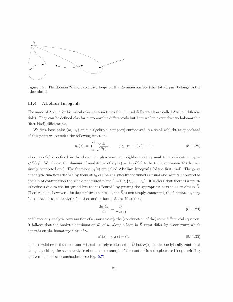
0Z
Figure 5.7: The domain D and two closed loops on the Riemann surface (the dotted part belongs to theother sheet).
11.4 Abelian Integrals
The name of Abel is for historical reasons (sometimes the 1st kind differentials are called Abelian differen-
tials). They can be defined also for meromorphic differentials but here we limit ourselves to holomorphic
(first kind) differentials.
We fix a base-point (w0, z0) on our algebraic (compact) surface and in a small schlicht neighborhood
of this point we consider the following functions
uj(z) :=
∫ z
z0
ζjdζ√P (ζ)
, j ≤ [(n− 1)/2]− 1 , (5.11.28)
where√P (ζ) is defined in the chosen simply-connected neighborhood by analytic continuation w0 =√
P (z0). We choose the domain of analyticity of w±(z) = ±√P (z) to be the cut domain D (the non
simply connected one). The functions uj(z) are called Abelian integrals (of the first kind). The germ
of analytic functions defined by them at z0 can be analytically continued as usual and admits unrestricted
domain of continuation the whole punctured plane C = C \ z1, . . . , zn. It is clear that there is a multi-
valuedness due to the integrand but that is ”cured” by putting the appropriate cuts so as to obtain D.
There remains however a further multivaluedness: since D is non simply-connected, the functions uj may
fail to extend to an analytic function, and in fact it does/ Note that
duj(z)
dz=
zj
w±(z), (5.11.29)
and hence any analytic continuation of uj must satisfy the (continuation of the) same differential equation.
It follows that the analytic continuation uj of uj along a loop in D must differ by a constant which
depends on the homotopy class of γ.
uj(z) − uj(z) = Cγ (5.11.30)
This is valid even if the contour γ is not entirely contained in D but w(z) can be analytically continued
along it yielding the same analytic element: for example if the contour is a simple closed loop encircling
an even number of branchpoints (see Fig. 5.7).
94
Definition 11.5 The constants Cγ defined in (5.11.30) are called the periods of the Abelian integrals.
We have
Proposition 11.3 Any period Cγ is a linear combination with integer coefficients of the fundamental
periods
Ωk,j := 2
∫ zj+1
zj
zkdz
w+(z)=
∮
γj
ωk , j = 1 . . . 2[(n− 1)/2]− 1, k = 0, . . . , [(n− 1)/2]− 1 (5.11.31)
where γj is a simple closed loop encircling the two branchpoints zj, zj+1 (note that te number of such
cycles is exactly twice the genus of the surfave).
The rectangular matrix Ω ∈ Mat(g × 2g,C) is called the (unnormalized) matrix of periods and plays
an essential role in the theory of Theta functions (topic for another course!).
The case of elliptic curve is a special case of these hyper-elliptic ones.
11.5 Symplectic basis in the homology
The definition of homology is beyond the scope of this course: for us here it is sufficient to say that the
(first) homology group is the abelian part of the homotopy group. It is a free abelian group on 2g (g is
the genus) generators and it is usually denoted additively.
The rationale is the following: if ω is a holomorphic differential, then the map
Iω : π1 → C (5.11.32)
[γ] → I([γ]) :=
∫
γ
ω (5.11.33)
is a group homomorphism between π1 and C (with addition). Namely
I([γ] · [γ′]) = I[γ] + I[γ′] (5.11.34)
Clearly it vanishes on [π1, π1] since
I([γ1] · [γ2] · [γ1]−1 · [γ2]
−1) = I([γ1]) + I([γ2]) − I([γ1]) − I([γ2]) = 0. (5.11.35)
Therefore it can be convenienetly thought of as a gruoup homomorphism from H1 := π1/[π1, π1] to C.
Elements of H1 are referred to as ”cycles”.
The group H1 is -as well as π1– generated by 2g generators. A convenient choice of generators is
to choose g ”a”-cycles and g ”b”-cycles in such a way as to make the representation of the intersection
number symplectic in this basis
ai♯aj = 0 = bi♯bj , ai♯bj = δij = −bj♯ai (5.11.36)
95
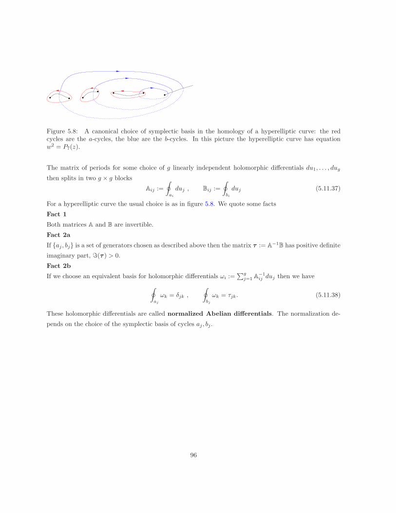
Figure 5.8: A canonical choice of symplectic basis in the homology of a hyperelliptic curve: the redcycles are the a-cycles, the blue are the b-cycles. In this picture the hyperelliptic curve has equationw2 = P7(z).
The matrix of periods for some choice of g linearly independent holomorphic differentials du1, . . . , dug
then splits in two g × g blocks
Aij :=
∮
ai
duj , Bij :=
∮
bi
duj (5.11.37)
For a hyperelliptic curve the usual choice is as in figure 5.8. We quote some facts
Fact 1
Both matrices A and B are invertible.
Fact 2a
If aj , bj is a set of generators chosen as described above then the matrix τ := A−1B has positive definite
imaginary part, ℑ(τ ) > 0.
Fact 2b
If we choose an equivalent basis for holomorphic differentials ωi :=∑g
j=1 A−1ij duj then we have
∮
aj
ωk = δjk ,
∮
bj
ωk = τjk. (5.11.38)
These holomorphic differentials are called normalized Abelian differentials. The normalization de-
pends on the choice of the symplectic basis of cycles aj , bj.
96
Chapter 6
Harmonic functions
1 Harmonic conjugate
Definition 1.1 Let u(x, y) : D → R be a C2(D) function (the second partial derivatives exist and are
continuous). The function is called harmonic if it satisfies Laplace’s equation
∇2u := ∂2xu(x, y) + ∂2
yu(x, y) = 0 . (6.1.1)
By identification z = x+ iy we will write u(z) although (clearly) f cannot be holomorphic; more properly
we will write u(z, z) if required for clarity. Recalling the definition of the differential operators ∂z, ∂z we
can rewrite Laplace’s equation as
∂z∂zu(z, z) = 0 (6.1.2)
Consider now a harmonic function u(z) and consider the one-form
ω := uydx− uxdy . (6.1.3)
This differential is closed because of harmonicity of u(x, y)
∂y(uy) = −∂x(ux) ⇔ ∇2u = 0 (6.1.4)
Therefore in any simply-connected subregion of D we can construct a C2 function v such that dv = ω:
explicitly this means that there is a C2 function v(x, y) such that
vx = uy , vy = −ux (6.1.5)
Definition 1.2 The function v is called the harmonic conjugate of the harmonic function u and it is
also harmonic where defined.
97
Explicitly, the formula for v is
v(z) =
∫ z
z0
(uydx− uxdy
)(6.1.6)
where the integral is independent of the path in the same homotopy class. If z is in a simply connected
neighborhood of z0 then the definition is unambiguous.
Suppose now that D itself is simply connected. Then v is defined and harmonic throughout D. The
equations defining v are precisely the Cauchy-Riemann equations for the complex–valued function
f(z) = u(x, y) + iv(x, y) , (6.1.7)
which is then holomorphic. In particular this implies that a harmonic function is in fact infinitely
differentiable (since so is f(z)). Viceversa, given a holomorphic function f ∈ H(D) (whether D is simply
connected or not), then its real and imaginary parts define harmonic functions for the CR equations give
f = u+ iv (6.1.8)ux = −vy
uy = vx⇒
uxx = −vxy = −uyy
vxx = uyx = −vyy(6.1.9)
and v is the harmonic conjugate of u. We have proved
Proposition 1.1 Given a harmonic function u on a domain D then for each simply connected sub-
domain Dsc ⊂ D there is a holomorphic function f whose real part coincides with u. Such holomorphic
function is uniquely defined up to addition of a purely imaginary constant.
Put it differently, any harmonic function defines at any point a germ of analytic function (modulo additive
imaginary constants) which admits unrestricted analytic continuation to D. The obstruction to the
existence of a harmonic conjugate is the same as the obstruction to the analytic continuation being a
holomorphic (single-valued) function.
2 Mean and maximum value theorems
Harmonic functions share many properties of holomorphic functions (clearly!)
Theorem 6.2.0 Let u : D → R be harmonic and Da(r) ⊂ D. Then
u(a) =1
2π
∫ 2π
0
u(a+ reiθ
)dθ (6.2.1)
Proof. Choose ǫ > 0 such that Da(r + ǫ) ⊂ D; this is a simply connected domain, hence we can define
the harmonic conjugate v so that u = ℜf . Then
f(a) =1
2iπ
∮
|z−a|=r
f(z)dz
z − a. (6.2.2)
98
If we parametrize the boundary z = a+ reiθ then
dz
z − a= idθ , (6.2.3)
and the formula follows taking the real part. Q.E.D.
Definition 2.1 (Mean value property for real functions) A function u : D → R is said to satisfy
the mean value property (MVP) if eq. (6.2.1) holds for all a ∈ D and radii r such that Da(r) ⊂ D.
Quite clearly this is just a rephrasing of Def. 5.2.
Proposition 2.1 [Maximum principle] If u : D → R is a continuous function satisfying the MVP, and
a ∈ D is a maximum
u(a) ≥ u(z) , (6.2.4)
then u(z) is identically constant.
Proof. Consider the set of maxima
M := z ∈ D : u(z) = u(a) . (6.2.5)
Since u is continuous this set is closed. We prove that is also open, and then –since D is connected–
M = D. Indeed let a0 ∈ M : we can find a small circle of radius r centered there and contained in Dwhere to apply the MVP. From the continuity it follows easily that
u(a0) =1
2π
∫u(z(θ))dθ ≤≤ max
|z−a|=ru(z) (6.2.6)
with the equaility iff u(z) is constant on the circle. Since r is arbitrary, it follows that u is constant in a
small disk centered at a0, hence M is open. Q.E.D.
Remark 2.1 If u is harmonic then so is −u, hence the maximum principle is also a minimum principle.
We now prove the equivalent of Cauchy’s integral formula for harmonic functions; we need to find the
analogue of dζζ−z . This analogoue is called the Poisson kernel.
Consider a disk D0(ρ). and define the following
P (ζ, z) :=|ζ|2 − |z2||z − ζ|2 (6.2.7)
Then we have
Theorem 6.2.7 (Integral formula for harmonic functions on the disk) Let u(z) be harmonic on
a domain containing |z| ≤ ρ; then, for all |z| < ρ we have
u(z) =1
2π
∮
|ζ|=ρ
u(ζ)P (ζ, z)dζ
iζ(6.2.8)
99
Proof. Let f be the holomorphic function defined on D0(ρ) whose real part is u. We want to ”massage”
Cauchy integral formula into the above
f(z) =1
2π
∮
|ζ|=ρ
f(ζ)ζ
ζ − z
dζ
iζ(6.2.9)
We add to this integral another one which is identically zero: namely let z⋆ be the reflection of z on the
circle
ζ⋆ :=ρ2
z, |z⋆| > ρ . (6.2.10)
Therefore
0 ≡ 1
2π
∮
|ζ|=ρ
f(ζ)ζ
ζ − z⋆
dζ
iζ(6.2.11)
Adding the two we have (note that ζζ = ρ2 = z z⋆)
ζ
ζ − z+
ζ
ζ − z⋆= P (ζ, z) . (6.2.12)
which is real valued. The proof now follows by taking the real part. Q.E.D
More generally one can prove
Theorem 6.2.12 Let φ(z) continuous and defined on |z| = ρ. Then
u(z) :=1
2π
∮
|ζ|=ρ
P (ζ, z)φ(ζ)dζ
iζ, (6.2.13)
is (the unique) harmonic function with continuous extension to the closed disk and boundary values given
by φ(z).
The fact that this function is harmonic is simple since P (z, ζ) is harmonic w.r.t. z. The slightly compli-
cated part is to prove that the boundary value of u is φ (we omit this part).
Theorem 6.2.13 Let u(z) : D → R satisfy the MVP. Then u is harmonic.
Proof. It is enough to show that u is harmonic in each disk. Choose a closed disk contained in D: define
w : D → R as the unique harmonic function whose boundary value on ∂D coincides with u. Since u−w
satisfies the MVP on the disk, then it also satisfies the maximum/minimum principle and since u−w ≡ 0
on the boundary, it follows that u ≡ w on the disk, and hence u is harmonic. Q.E.D.
.
100
Chapter 7
Riemann mapping theorem
1 Statement
We are now going to prove the following result, going under the name of Riemann’s mapping theorem.
Theorem 7.1.0 (Riemann’s mapping theorem) Every simply connected domain D ⊂ C, D 6= C is
biholomorphic to the unit disk D := |z| < 1
The proof requirese quite some preparations.
Lemma 7.1.0 Given a simply connected domain D 6= C then there is a biholomorphic mapping to a
bounded domain B.
Proof. Let a 6∈ D and choose arbitrarily and fix z0 ∈ D. Then
g(z) :=
∫ z
z0
dζ
ζ − a= ln(z − a) − ln(z0 − a) (7.1.1)
is well defined globally on D because of the simple-connectivity. By analytic continuation of the identity
eg(z) =z − a
z0 − a, (7.1.2)
valid in a neighborhood of z0, we see that g(z) is univalent and hence establishes a biholomorphic mapping
between D and g(D). We claim that
T := g(D) ∩ (g(D) + 2iπ) = ∅ (7.1.3)
Indeed suppose that w ∈ T : then there are two distinct points z1, z2 with g(z1) = g(z2) + 2iπ; this
however means that |z1 − a| = |z2 − a| and arg(z1 − a) = arg(z2 − a) + 2π, which implies that z1 = z2,
a contradiction. We also claim that there is a positive ǫ > 0 such that |g(z) − 2iπ| > ǫ: indeed suppose
101
that there is a sequence zn ∈ D such that g(zn) → 2iπ. This sequence would necessarily converge to z0
forzn − a
z0 − a= eg(zn) → 1 . (7.1.4)
But this is impossible since g(z) is a biholomorphism in a neighborhood of z0. Consider then the function
G(z) :=1
g(z) − 2iπ. (7.1.5)
Then we have |G(z)| < 1ǫ and it is still a biholomorphism between D and G(D), which is bounded. Q.E.D.
This lemma shows that without loss of generality we may assume (up to a dilation) that D ⊂ D. By
possibly a small translation we can also assume that 0 ∈ D. The crucial point is that a biholomorphic
equivalence between such a D and D has a certain extremal property described in the following theorem.
Theorem 7.1.5 Let M be the set of univalent holomorphic maps f : D → D, where D ⊂ D is a simply
connected domain containing z = 0 and such that f(0) = 0. A map ϕ : D → D with ϕ(0) = 0 is a
biholomorphic equivalence if and only if
∀f ∈ M , |f ′(0)| ≤ |ϕ′(0)| . (7.1.6)
Proof. The set M is nonempty since the identity map belongs to it. Suppose ϕ is a biholomorphic
equivalence with the stated properties and f : D → D a univalent map. Let
h := f ϕ−1 : D → D ⊂ D . (7.1.7)
Note that h(0) = 0 We claim that |h′(0)| ≤ 1, indeed ∀ǫ > 0
|h′(0)| =
∣∣∣∣∣1
2iπ
∮
|z|=1−ǫ
h(z)
z2dz
∣∣∣∣∣ ≤supz∈D
|h(z)|1 − ǫ
≤ 1
1 − ǫ(7.1.8)
Taking the inf w.r.t. ǫ yields the result. From the chain rule we have then
∣∣∣∣f ′(0)
ϕ′(0)
∣∣∣∣ ≤ 1 (7.1.9)
which proves the necessity.
In order to prove the sufficiency we must prove that if ϕ : D → D is univalent with ϕ(0) = 0 and has
the claimed extremal property then it is onto. So let ϕ such a function and suppose it is not onto. Let
a ∈ D such that a 6∈ ϕ(D). We then construct a function g ∈ M with |g′(0)| > |ϕ′(0)|.
102
Construction of g(z). We define
ψ(z) =ϕ(z) − a
1 − aϕ(z): D → D (7.1.10)
since this linear/fractional transformation is a map of D into itself. So now we have a ψ(z) : D → D
which never vanishes. We can define unambiguously
H(z) := lnψ(z) : D → D (7.1.11)
since D is simply connected and ϕ(z) is never zero. Note that ℜH(z) < 0 since |ψ(z)| < 1. We set
g(z) =H(z) −H(0)
H(z) +H(0)(7.1.12)
and claim that this function yields a contradiction with the hypothesis of extremality. First of all we
must check that g ∈ M: indeed g(0) = 0 and
|g(z)| =
∣∣∣∣H −H0
H +H0
∣∣∣∣ < 1 (7.1.13)
since the distance of H0 from H is less than the distance of −H0 (which has same imaginary part as H0).
We finally compute
g′(0) =H ′(0)
H(0) +H(0), H ′(0) =
(a− 1
a
)ϕ′(0) , H(0) = ln(−a) (7.1.14)
g′(0) =
(a− 1
a
)1
ln(|a|2)ϕ′(0) (7.1.15)
hence ∣∣∣∣g′(0)
ϕ′(0)
∣∣∣∣ =|a|2 − 1
|a| ln(|a|2) (7.1.16)
It is then an exercise to see that the function of |a| on the RHS is strictly greater than 1 on the interval
0 < |a| < 1. Q.E.D.
The only missing step now is to show existence of an extremal map ϕ; the idea is that of endowing
the set M with a topology such that it is (a) compact and (b) the function
δ′0 : M → R , δ′0(f) := |f ′(0)| (7.1.17)
is continuous and bounded. Then it must have a maximum on this set. This requires the study of the
topology of H(D).
103
2 Topology of H(D)
The vector space H(D) is a subspace of the continuous maps, for which we have the sup norm. The small
problem is that D is not compact and hence we must introduce a work-around.
Recall that if (X, d) is a compact metric space, the vector space of continuous functions
C(X) := f : X → C , f continous (7.2.1)
is endowed with the distance
δ(f, g) := supx∈X
|f(x) − g(x)| = maxx∈X
|f(x) − g(x)| . (7.2.2)
The metric space (C(X), δ) is then a complete metric space (i.e. any Cauchy sequence converges to a
continuous function).
Let now D ⊂ C be an open set.
Lemma 7.2.2 There is a collection Knn∈N of compact subsets of D such that
1.⋃
n∈N
Kn = D
2. Kn ⊂Kn+1
3. ∀C ⊂ D, C compact there is N such that C ⊂ Kn.
Such a sequence of increasing compact sets is called a saturating sequence.
Proof. We define
Kn := |z| ≤ n ∩z ∈ D s.t. d(z,C \ D) ≥ 1
n
(7.2.3)
Note that d(z,C \ D) for z ∈ D is defined as
d(z,Dc) := infw 6∈D
|z − w| (7.2.4)
and the sets d(z,Dc) ≥ x are all closed sets. Indeed if zn ⊂ D is a Cauchy sequence such that
d(zn,Dc) ≥ x > 0 then the limit point z∞ also has the property d(z∞,Dc) ≥ x and hence belongs to D(the disk Dz∞(x/2) has no intersection with Dc and hence belongs to D).
The sets Kn are therefore closed and bounded in C and hence compacts. The rest of the proof is left
as exercise. Q.E.D.
Let now Kn be such a saturating sequence of compacts in D. Define
ρn(f, g) := maxz∈Kn
|f(z) − g(z)| . (7.2.5)
and then
ρ(f, g) :=
∞∑
n=1
2−n ρn(f, g)
1 + ρn(f, g). (7.2.6)
We claim that ρ is a metric on C(D), indeed
104
1. If ρ(f, g) = 0 then all ρn(f, g) = 0 and hence f ≡ g (and viceversa obviously).
2. Trivially ρ(f, g) = ρ(g, f).
3. ρ(f, g) ≤ ρ(f, h) + ρ(h, g) because the same is true for all ρn’s.
The convergence in the metric ρ is such that a sequence fn converges to f iff the sequence converges
uniformly on all compact sets K ⊂ D. Since uniform convergence on a compact set is sufficient
to guarantee continuity, the space (C(D), ρ) is complete. In the metric ρ the space C(D) is of finite
diameter, therefore the notion of bounded set is slightly different
Definition 2.1 A set B ⊂ C(D) is called bounded if all elements of B are uniformly bounded on any
compact subset K ⊂ D; Being bounded in ρ means that the functions in M are uniformly bounded on
any compact set
∀K ⊂ D,K compact , ∃M s.t. ∀f ∈ B supz∈K
|f(z)| < M . (7.2.7)
Theorem 7.2.7 The subspace H(D) ⊂ C(D) is closed (hence complete) in the metric ρ of uniform
convergence on compact sets.
Proof. Let fn be a Cauchy sequence of holomorphic functions: we know that f∞ is at least continuous.
To prove that it is holomorphic at all points choose a small circle γ contained in D. Note that γ is a
compact set and hence we have uniform convergence on the points of γ. Then for all z inside this disk
fn(z) =1
2iπ
∮
γ
fn(ζ)dζ
ζ − z(7.2.8)
Passing to the limit on the RHS and LHS we have a similar Cauchy integral representation for f∞ which
is therefore holomorphic in the (arbitrary) disk. Q.E.D.
Theorem 7.2.8 The map
D : H(D) → H(D) , D(f)(z) := f ′(z) , (7.2.9)
is continuous. Moreover it maps any bounded set M ⊂ H(D) into a bounded set.
Proof. We need to prove that if fn → f in the metric ρ then f ′n → f ′ in the metric ρ or, equivalently
that we have uniform convergence on any compact K ⊂ D of f ′n.
Note that –since any compact is covered by a finite number of disks contained in D, it is sufficient to
verify the uniform convergence on an arbitrary disk Da(R) ⊂ D. To do this we need to take a slightly
larger disk such that its closure is still in D, namely we choose ǫ > 0 such that Da(R+ ǫ) ⊂ D. Then for
z ∈ Da(R)
|f ′n(z) − f ′(z)| =
1
2π
∣∣∣∣∣
∮
|w−a|=R+ǫ
(fn(w) − f(w))dw
(w − z)2
∣∣∣∣∣ ≤1
2π
∮
∂Da(R+ǫ)
|fn(w) − f(w)||z − w|2 ds ≤ (7.2.10)
≤ supz∈Da(R+ǫ)
|f(z) − fn(z)|R+ ǫ
ǫ2−→
n→∞0 (7.2.11)
105
This proves the continuity. For the boundedness let M be a bounded set of holomorphic functions on
D. Once more it is sufficient to check the assertion for disks. Using the same disks as before and letting
M be the bounding constant on the set Da(R+ ǫ), we have easily that D(M) is bounded on the disk
Da(R),
|f ′(z)| ≤MR
ǫ2. (7.2.12)
Q.E.D.
Proposition 2.1 The evaluation map eva : H(D) → C, eva(f) = f(a) is continuous.
Proof. Uniform convergence implies pointwise convergence. Q.E.D.
Composing the differentiation with the evaluation we have that the map Da(f) = f ′(a) is a continuous
map, and so is |f ′(a)|.In particular we have
Corollary 7.2.12 For a uniformly convergent sequence fn ∈ H(D) all derivatives at any point of D are
convergent sequences. Viceversa a sequence fn ∈ H(D) is uniformly convergent on any compact K ⊂ Dif all the derivatives at all points are convergent and the sequence is bounded (i.e. uniformly bounded
on compact sets).
Proof. Only the ”viceversa” part is not already proved. Once more it is sufficient to verify the statement
for an arbitrary disk Da(r) ⊂ D. So let fn be such a sequence. Fix a ∈ D and let r < R such that
Da(R) ⊂ D. Let M be the bounding constant for the sequence on this compact. We have
|f (k)n (a)| ≤ k!
2π
∮
|z−a|=R
∣∣∣∣fn(z)dz
(z − a)k+1
∣∣∣∣ ≤k!M
Rk(7.2.13)
Let us estimate the distance on the disk of radius r, |z − a| ≤ r
|fn(z) − fm(z)| ≤N∑
k=0
|f (k)n − f
(k)m |
k!|z − a|k +
∑
k>N
|f (k)n − f
(k)m |
k!rk ≤ (7.2.14)
≤S∑
k=0
|f (k)n − f
(k)m |
k!rk + 2M
∑
k>S
( rR
)k
(7.2.15)
Fix ǫ > 0: since the last geometric series is convergent there is S0 such that S > S0 implies that the last
term is less than ǫ/2. Since the first term contains only a finite number of convergent sequences (and S0
terms), then there is a N = N(S0) such that for n,m > N the first sum is less than ǫ/2. Hence we have
the uniform convergence. Q.E.D.
In order to be able to complete the proof of Riemann’s mapping theorem we need to find a compact
set in our M. We have
106
Theorem 7.2.15 A set M ⊂ H(D) is compact iff it is closed and bounded.
Proof. Let M be compact. Then it is obviously closed. The boundedness is almost obvious: let K ⊂ Dbe a compact set. The function
‖f‖K := maxz∈K
|f(z)| (7.2.16)
is continuous and hence has a maximum for f0 in M. This maximum cannot be infinite and hence M is
bounded.
The nontrivial direction is the proof that boundedness+closedness implies compactness. Let then Mbe closed and bounded and let fn a sequence in M: we need to find a convergent subsequence, namely
a subsequence that converges uniformly on all compacts.
We first find a uniformly convergent subsequence on a arbitrary but fixed compact set K ⊂ D. By
compactness, this set can be covered by a finite number of disks whose closure still is contained in D. Let
a be the center of one of these finite disks and R its radius. For k ∈ N fixed, each sequence f (k)n (a)n∈N
is bounded and hence admits a convergent subsequence. Let N0 be the subsequence for k = 0. From
this one we can extract another subsequence N1 ⊂ N0 for which f ′n(a) converges. From this one we can
extract another subsequence N2 ⊂ N1 for which f ′′n (a) converges. And so on and so forth.
We then extract the ”diagonal” subsequence, namely nℓ is the ℓ-th element of Nℓ: since the subse-
quences are nested, nℓ is a subsequence of Nℓ0 for ℓ > ℓ0. In particular this implies that for any ℓ0 ∈ N
the sequence f(ℓ0)nℓ (a) converges as ℓ→ ∞. By Corollary 7.2.12 this subsequence converges uniformly on
the disk Da(r), for any r < R. We repeat this procedure for the finite number of disks that cover K
and note that if the finite disks Dai(Ri) cover K so do the Dai
(Ri − ǫ) for some small enough ǫ > 0.
Therefore we have uniform convergence on K.
To complete the proof we take a saturating sequence of compact sets Kν, ν ∈ N; for each of them
there is a convergent subsequence fnℓas before. We repeat the diagonal argument by constructing nested
subsequences and reading them on the diagonal, and thus complete the proof. Q.E.D.
We will need also a result of Hurwitz
Proposition 2.2 [Hurwitz’s Theorem] Let fn ⊂ H(D) be a sequence uniformly convergent to f ∈H(D) on compact sets. Let Da(R) ⊂ D be such that f(a) 6= 0: then ∃N ∈ N s.t. ∀n > N the functions
fn have the same number of zeroes in Da(R) as f does.
Proof. The number of zeroes of fn in the closed disk is
1
2iπ
∮
|z−a|=R
f ′n(z)dz
fn(z)(7.2.17)
and a similar expression for f . If a zero of f happens to be exactly on the boundary of the chosen closed
disk, we slightly enlarge it R′ = R+ ǫ in such a way as to not include any further zero (this is possible
107
since the zeroes of a holomorphic function is discrete in its domain). We will therefore assume that no
zero of f falls exactly on the boundary. We know that both fn and f ′n are uniformly convergent on any
compact set to f and f ′: since f(z) 6= 0 on the circle |z − a| = R then also
min|z−a|=R
|f(z)| = δ > 0 , (7.2.18)
and there is N ′ ∈ N such that |fn(z)| ≥ δ/2 on |z− a| = R for n ≥ N ′. Moreover we have for |z− a| = R∣∣∣∣f ′
n
fn− f ′
f
∣∣∣∣ =∣∣∣∣f ′
nf − f ′fn
ffn
∣∣∣∣ =
∣∣∣∣f ′
nf − f ′f + f ′f − f ′fn
ffn
∣∣∣∣ ≤∣∣∣∣f ′
n − f ′
fn
∣∣∣∣+∣∣∣∣f ′(f − fn)
ffn
∣∣∣∣ (7.2.19)
Since the numerators are bounded away from zero and the numerators tend to zero we have N such that
n > N implies ∣∣∣∣f ′
n
fn− f ′
f
∣∣∣∣ ≤1
2R. (7.2.20)
Then the difference of the number of zeroes is less than 12 and hence they must be the same (since they
must be integers). Q.E.D.
Corollary 7.2.20 If fn : D → C is a sequence of univalent maps uniformly convergent on compact sets
K ⊂ D to f , then either f is a constant or else f is univalent as well.
Proof. Suppose f not constant and suppose it is not univalent. Let z1, z2 ∈ D such that f(z1) =
f(z2) = a. Then fn(z) − a must also have zeroes in suitable neighborhoods of z1, z2 for n large enough,
contradicting the univalency. Q.E.D.
3 Proof
Proof of Thm. 7.1.0. Recall that D ⊂ D is a simply-connected domain and M is the set of
holomorphic univalent maps f : D → D fixing the origin f(0) = 0. We have established that the map
achieving the equivalence is the one for which |f ′(0)| is maximal in M.
The set M is clearly bounded. We also know from Corollary 7.2.20 that a Cauchy sequence in Meither converges in M or converges to a constant (which actually must be 0) . We must exclude this
possibility. Consider the subsets
Mr := f ∈ M : |f ′(0)| ≥ r . (7.3.1)
These sets are still bounded and moreover closed because the function |f ′(0)| is continuous. Since f(z) = z
belongs to M then Mr are certainly nonempty for 0 < r ≤ 1. A convergent sequence in Mr cannot
converge to a constant and it is easy to see (from the continuity of |f ′(0)|) that converges within Mr.
In view of Thm. 7.2.15 then Mr is compact; the continuous functional
δ′ : Mr → R , δ′(f) := |f ′(0)| (7.3.2)
must have a point ϕ ∈ Mr of maximum. This map is the required equivalence. Q.E.D.
108
4 Extensions of the theorem
Riemann’s theorem can be significantly extended to the following situation: let L be a compact one-
dimensional complex manifold. It can be shown that it is (equivalent) to (the compactification of ) an
algebraic curve.
Let L be its universal covering: unless L is simply connected to begin with, L is not compact. Let g
be the genus of this curve; we recall that we have defined it to be the dimension of the space of first-kind
differentials (holomorphic one-forms). There are more ”geometric” but equivalent definitions which we
omit. We have
Proposition 4.1 Let g ≥ 1 and fix p0 ∈ L. There are 2g closed simple curves γj whose homotopy classes
generate the fundamental group π1(L, p0) and such that D := L \⋃2gj=1 γj is a simply-connected domain.
Furthermore these generators satisfy a single group-relation in the fundamental group π1(L)
[γ1] · [γ2] · · · [γ2g] = 1 (7.4.1)
The extension of Riemann’s theorem is the following
Theorem 7.4.1 Let L be the universal covering of an algebraic compact curve L of genus g. Then there
is a univalent holomorphic map ϕ which establishes a biholomorphic equivalence of L with the following
domains
1. The Riemann sphere C if g = 0.
2. The complex plane C is g = 1.
3. The upper half plane H+ if g ≥ 2.
These three cases are called (confusingly), elliptic (g = 0), parabolic (g = 1) or hyperbolic (g ≥ 2).
Since the deck transformations of L act properly-discontinuously on L, then their composition with the
biholomorphic equivalence ϕ also has the same property. Let Γ be the group of such deck transformations.
Then we know that L/Γ ≃ L (basically by definition of universal covering). Therefore
Theorem 7.4.1 Any one-dimensional compact (connected) complex manifold is biholomorphically equiv-
alent to the quotient of C or H+ for the cases g = 1, g ≥ 2 respectively, by a group of automorphisms of
C or H+ respectively which acts properly-discontinuously.
The proof (cf. Siegel) is quite involved and goes along these points.
Let U be a connected, simply connected one dimensional manifold (usually the universal cover of a
compact curve). Prove the existence of a meromorphic functiion f(ζ) which
1. f(ζ) has only one simple pole with residue 1 at some point ζ0.
2. f(ζ) minimizes a Dirichlet integral.
Using the minimum property one is able to show that f(ζ) is univalent and performs the requested
equivalence.
109

4.1 Some conformal mappings
There is an endless list of type of domains for which the explicit conformal mapping has been worked
out, the reason being their interest in problems of 2-dimensional, irrotational stationary fluid dynamics.
Just one example is the following.
Schwarz–Christoffel transformations
These give the conformal map of an arbitrary polygon to the upper half plane (or rather the viceversa).
Let x1 < x2, . . . , xn ∈ R and a1, a2, . . . , an ∈ (0, 2π). Let
dw
dz= A
n∏
j=1
(z − xj)ajπ
−1 , ℑz > 0, A 6= 0 . (7.4.2)
Then w(z) establishes a biholomorphic equivalence between the upper half z–plane and the interior of a
polygon with interior angle aj at the wj vertex. Note that the polygon may be degenerate if we allow
aj = 0, 2π and it may also be non closed.
5 Exercises
In this section we mean by ”equivalence” a biholomorphic mapping. The unit disk will be denoted by
D := |z| < 1 , (7.5.1)
and the upper half plane by
H+ := z : ℑ(z) > 0 . (7.5.2)
Exercise 5.1 Let D and D be simply-connected domains in C with D bounded. Let f : D → C be
holomorphic on D and continuous on D (the closure) and such that f : ∂D → ∂D gives a piecewise
smooth correspondence between the oriented boundaries. Prove that f is onto (surjective).
Exercise 5.2 Find an equivalence of the following domain with the unit disk D.
D :=z = x+ iy : y2 > 4(x+ 1)
(7.5.3)
Exercise 5.3 Construct an equivalence of the upper half plane with a cut
D := z : ℑ(z) > 0 \ [a, a+ ih] , a, h ∈ R , h > 0 , (7.5.4)
(where [a, a+ ih] denotes a straight segment) with the upper half plane H+ without the cut.
110
Chapter 8
Picard’s theorems
1 Picard’s Little Theorem
We have
Theorem 8.1.0 (Picard’s little theorem) Let f be an entire function such that it omits two values.
Then f is a constant.
Consider an elliptic curve
Y 2 = 4X3 − g2X − g3 , g23 − 27g3
2 6= 0 , (8.1.1)
and denote by e1, e2, e3 the roots (which are distinct!). We already know that the compactification of this
curve if equivalent to the manifold C/(ω1Z + ω2Z) where the periods ωi are defined by certain elliptic
integrals. We also know that these lattices are equivalent if the modular parameters τ = ω1
ω2are related
by the transformations
τ 7→ aτ + b
cτ + d,
(a bc d
)∈ SL2(Z) . (8.1.2)
In fact we have also proved that it suffices to look at the modular invariant
J(τ) :=g2
3
g23 − 27g32(8.1.3)
and this unique number characterizes the classes of elliptic curves.
Note that the algebraic curve
Y 2 = 4X3 − κ4g2X − κ6g3 (8.1.4)
has the same modular invariant and hence is equivalent (it is sufficient to rescale Y 7→ κ3Y and X 7→κ2X). The roots are now e′i = κ−2ei. We define
λ :=e1 − e2e3 − e2
6= 0, 1 (8.1.5)
111
Under a modular transformation
ω′1 = aω1 + bω2 (8.1.6)
ω′2 = dω1 + cω2 (8.1.7)(
a bc d
)∈ SL2(Z) (8.1.8)
the half periods σi (i = 1, 2, 3) in general are permuted
σ′1 =
a
2ω1 +
b
2ω2 (8.1.9)
σ′2 =
c
2ω1 +
d
2ω2 , (8.1.10)
depending on the class of a, b, c, d mod 2. They are not permuted iff(a bc d
)≡(
1 00 1
)mod 2 (8.1.11)
because in this case the new half periods are equivalent to the old ones by a shift in the lattice. Trans-
formations of these type constitute a subgroup of SL2(Z) denoted
Γ2 :=
g =
(a bc d
)∈ SL2(Z) : g = 1 mod 2
. (8.1.12)
Proposition 1.1 The group Γ2 is generated by the transformations
± 1, α =
(1 20 1
)= T 2 , β =
(0 12 1
)= −ST 2Sα(τ) = τ + 2 , β(τ) =
τ
2τ + 1(8.1.13)
and has fundamental domain depicted in Fig. 8.1.
Proof. Consider the group
G :=
(a bc d
), a, b, c, d ∈ Z2 : ab− cd = 1
= SL2(Z2) . (8.1.14)
(That this is a group is left as exercise). This is a finite group of Mat(2× 2,Z2) (which has 16 elements),
with elements
1, e =
(1 10 1
), f =
(1 01 1
), g =
(0 11 0
), h =
(0 11 1
), ℓ =
(1 11 0
)(8.1.15)
with the following multiplication table:
1 e f g h ℓ1 1 e f g h ℓe e 1 h ℓ f gf f ℓ 1 h g eg g h ℓ 1 e fh h g e f ℓ 1ℓ ℓ f g e 1 h
(8.1.16)
112
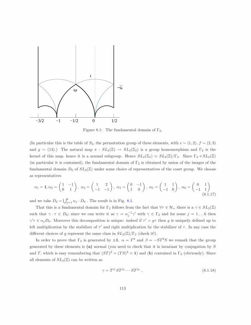
i
ω −ω
−1/2 0 1/2−1−3/2
Figure 8.1: The fundamental domain of Γ2.
(In particular this is the table of S3, the permutation group of three elements, with e ∼ (1, 2), f ∼ (2, 3)
and g ∼ (13).) The natural map π : SL2(Z) → SL2(Z2) is a group homomorphism and Γ2 is the
kernel of this map, hence it is a normal subgroup. Hence SL2(Z2) ≃ SL2(Z)/Γ2. Since Γ2 ⊳ SL2(Z)
(in particular it is contained), the fundamental domain of Γ2 is obtained by union of the images of the
fundamental domain D0 of SL2(Z) under some choice of representatives of the coset group. We choose
as representatives
α1 = 1, α2 =
(1 −10 1
), α3 =
(1 2−1 −1
), α4 =
(0 −11 0
), α5 =
(1 1−1 0
), α6 =
(0 1−1 1
)
(8.1.17)
and we take D2 =⋃6
j=1 αj ·D0 . The result is in Fig. 8.1.
That this is a fundamental domain for Γ2 follows from the fact that ∀τ ∈ H+ there is a γ ∈ SL2(Z)
such that γ · τ ∈ D0; since we can write it as γ = α−1j γ′ with γ ∈ Γ2 and for some j = 1 . . . 6 then
γ′τ ∈ αjD0. Moreover this decomposition is unique: indeed if τ ′ = gτ then g is uniquely defined up to
left multiplication by the stabilizer of τ ′ and right multiplication by the stabilizer of τ . In any case the
different choices of g represent the same class in SL2(Z)/Γ2 (check it!).
In order to prove that Γ2 is generated by ±1, α = T 2 and β = −ST 2S we remark that the group
generated by these elements is (a) normal (you need to check that it is invariant by conjugation by S
and T , which is easy remembering that (ST )3 = (TS)3 = 1) and (b) contained in Γ2 (obviously). Since
all elements of SL2(Z) can be written as
γ = T j1ST j2 · · ·ST jk , (8.1.18)
113
we can pull to the right the even powers of T 2k = αk and of ST 2kS = ±βk, leaving on the left one of the
following words
1, T−1, S−1, (TS)−1, (ST )−1, TS−1T−1 , (8.1.19)
which are the αj . Hence the two quotients have the same classes and hence the group generated by
±1, α, β coincides with Γ2. Note also that the action of Γ2 has no points with nontrivial stabilizer (i.e.
bigger than ±1 in this case). Q.E.D.
Given that ei = ℘(ωi/2) it is easy to see that λ(ω1, ω2) depends in fact only on their ratio τ . From
the previous discussion it should be clear also that λ(τ) is invariant under Γ2:
λ(τ + 2) = λ(τ) λ
(τ
2τ + 1
)= λ(τ) . (8.1.20)
and cannot take the values 0, 1. It can take any other value for in this case we can set e.g.
e1 = κ(1 − 2λ) , e2 = κ(1 + λ), e3 = −e1 − e2 (8.1.21)
and these are all the numbers with the prescribed λ. It is also easy to see that if two algebraic curves
have the same λ (up to a permuation of the roots) then they have the same J : in fact
Exercise 1.1 (Check!) Prove that the modular invariant J is related to λ by
J =4(1 − λ+ λ2)3
27λ2(1 − λ)2(8.1.22)
Prove that this expression is invariant under the transformations
λ 7→ λ
λ− 1, λ 7→ 1 − λ (8.1.23)
which corresponds to permutations of the three roots.
It also follows that if λ(τ) = λ(τ ′) then τ and τ ′ must be related by a transformation in Γ2 because
the two elliptic curves have the same half periods, (and clearly the viceversa is true as well). Since the
group Γ2 acts properly and discontinuously on H+ with trivial stabilizer, then λ(τ) is locally a univalent
map and hence
Proposition 1.2 The function λ(τ) : H+ → C \ 0, 1 is unramified and onto.
2 Proof of Thm. 8.1.0
The theorem can be rephrased as
Theorem 8.2.0 Given an entire non-constant function f(z), then f(z) takes on all values except possibly
one.
114
Proof. Suppose f does not take on the values a, b. By the transformation
f(z) =f(z) − a
b− a, (8.2.1)
we can always assume that a = 0, b = 1. Consider then the Riemann surface
λ(τ) = f(z) , τ ∈ λ−1(f(z)) (8.2.2)
This defines a covering of H+ onto C \ 0, 1: the number of sheets is infinite since all τ related by a
transformation of Γ2 have the same λ value.
Take z0 and τ0 ∈ λ−1(f(z0)); we can define a germ of analytic function τ(z) such that τ(z0) = τ0.
Since λ is a local equivalence, this germ admits unrestricted analytic continuation to the whole z plane
and since this is simply connected then this analytic continuation defines an analytic function (in fact
entire).
Consider finally
G(z) :=τ(z) − i
τ(z) + i(8.2.3)
Since ℑ(τ(z)) > 0 then |G(z)| < 1 and hence it is an entire, bounded function. Therefore G(z) is constant,
which can be iff f(z) is constant, a contradiction. Q.E.D.
3 Picard’s great theorem
Here we cheat a bit: we state without proof the following theorem.
Theorem 8.3.0 (Montel-Charateodory Theorem) Let D be a domain and F be the family of func-
tions that never assume the values 0, 1: then F is relatively compact in C(D,C), namely any sequence of
functions admits a subsequence which is either uniformly convergent on all compact subsets of D or else
uniformly tends to ∞ on any compact.
This is all we need to prove
Theorem 8.3.0 (Picard’s great theorem) Let f(z) have an essential singularity at z = a. In each
neighborhood of a f(z) assumes all complex values -except possibly one- infinitely many times.
Proof. Up to translation we can assume that the essential singularity is at z = 0. Suppose there is
R > 0 and two numbers a, b (which we assume to be 0, 1 up to a shift/rescaling of f) which are never
assumed in the punctured disk of radius R, D = D0(R) \ 0. Construct the sequence
fn(z) = f( zn
), n ≥ 1 (8.3.1)
This family is never assumes the values 0, 1 and hence admits a subsequence fnkwhich either converges
to an analytic function ϕ or converges uniformly to ∞ on all compact subsets of D.
115
If we are in the first case we set
M := max|z|=R/2
|ϕ(z)| (8.3.2)
From the uniform convergence it follows that on |z| = R/2
∣∣∣∣f(z
nk
)∣∣∣∣ ≤∣∣∣∣f(z
nk
)− ϕ(z)
∣∣∣∣+ |ϕ(z)| < M + 1 (8.3.3)
for nk sufficiently large. Therefore f(z) is uniformly bounded on concentric circles of radii R/(2nk) and
by the maximum modulus theorem it must be bounded on D. Hence z = 0 is a removable singularity, a
contradiction.
If ϕ ≡ ∞ then it is left as exercise to show that f(z) has a pole. Q.E.D.
116


![mypage.concordia.camypage.concordia.ca/mathstat/lpopovic/axonalfinal.pdfhyperbolic systems [17] [24] matical Statistics, John Wiley & Sons, Chichester, UK, 1979. Stochastic Analysis,](https://img.pdfslide.us/doc/110x75/5e58e048ad4801615223cc61/hyperbolic-systems-17-24-matical-statistics-john-wiley-sons-chichester.jpg)