Embed Size (px)
Citation preview
University of Central Florida
Electronic Theses and Dissertations Doctoral Dissertation (Open Access)
Competitive Actions Of New Technology FirmsThe Red Queen Effect And New Firm Performance2010
Robert L. PorterUniversity of Central Florida
Find similar works at: http://stars.library.ucf.edu/etd
University of Central Florida Libraries http://library.ucf.edu
This Doctoral Dissertation (Open Access) is brought to you for free and open access by STARS. It has been accepted for inclusion in Electronic Thesesand Dissertations by an authorized administrator of STARS. For more information, please contact [email protected].
STARS Citation
Porter, Robert L., "Competitive Actions Of New Technology Firms The Red Queen Effect And New Firm Performance" (2010).Electronic Theses and Dissertations. 1661.http://stars.library.ucf.edu/etd/1661

COMPETITIVE ACTIONS OF NEW TECHNOLOGY FIRMS: THE RED QUEEN
EFFECT AND NEW FIRM PERFORMANCE
by
ROBERT L. PORTER
B.S.E. University of Central Florida, 1981
M.B.A. Crummer School of Business, Rollins College, 1990
A dissertation submitted in partial fulfillment of the
requirements for the degree of Doctor of Philosophy
in the Department of Management
in the College of Business Administration
at the University of Central Florida
Orlando, Florida
Fall Term 2010
Major Professor: Cameron Ford
ii
ABSTRACT The competitive strategy used by a new firm may be the most important strategy it ever
employs (Covin & Slevin, 1989; Ferrier, 2001). A well-chosen and executed firm strategy is
essential for a firm to realize its potential competitive advantage (Porter, 1981). A firm‘s
strategic intent and resulting competitive actions are especially important when firms are new
and vulnerable as they strive to learn which strategic actions help them adapt to their rivals
actions and to their environment (Stinchcombe, 1965). Further, the competitive actions that new
firms choose to take with rival firms affects the overall competitive dynamics of their industry
(Smith, Ferrier, and Ndofor, 2001).
One way to explore how the competitive actions of new firms affect their future is to
capture and examine their individual competitive moves and countermoves over time (Smith,
Grimm, Gannon, & Chen, 1991). Red Queen competition is a particular form of competitive
dynamics that is well-suited to explore these issues of new rival firms (Barnett, 2008). Barnett
and Sorenson (2002) suggested that competition and learning reinforce one another as
organizations develop, and this is what van Valen (1973) referred to as the ‗Red Queen.‘ This
definition of the Red Queen led to the development of the concept of Red Queen competition and
the Red Queen effect. The competitive strategies these new firms use to obtain resources as they
adapt, in particular how these firms compete and or cooperate, are key competitive strategies that
remain understudied to-date (Amit, Glosten, and Muller, 1990).
I explore Red Queen competition, and the ensuing Red Queen Effect, in a complex
environmental setting that represents a high technology ecosystem (Arned, 1996, 2010; Iansiti &
Levien, 2004a, 2004b; Moore, 1993; Pierce, 2009). New firms in such an ecosystem represent a
particularly salient combination of type of firm, firm lifecycle period, and firm environment to
iii
examine strategic actions since these firms comprise a significant portion of the high-growth and
future of our global economy (Stangler, 2010). Further, due to their need to rapidly adapt in a
complex ecosystem, these firms rely heavily on short-lived information resources for competitive
advantage (Barney, 1991; Nelson and Winter, 1982; Omerzel, 2008). To place this research in
context, I consider the moderating effects of key environmental ecosystem resource conditions
(Dess & Beard, 1984; Miller & Friesen, 1983; Sharfman & Dean, 1991).
Empirical studies to-date have yielded mixed results and left unanswered questions about
the basic components and the effects of Red Queen competition. To address these issues I
explore this literature in chapter one of the dissertation, and in chapter two I develop a theoretical
model of Red Queen competition that draws on the available empirical and theoretical literature
to-date. Due to the mixed finding from the empirical results, I develop a precise agent-based
simulation model of Red Queen competition in chapter three to facilitate data collection. Using
this data I test a series of hypotheses designed to explore the fundamentals of Red Queen
competition, specifically how escalating competitive activity for resources among new firms
impacts their survival and performance. In addition, the moderating effect of environmental
changes on Red Queen competition is also tested to explore the affect of context on Red Queen
competition. Chapter four explains the findings from these hypotheses, future research
directions, implications and limitations from the research, and my concluding thoughts.

iv
ACKNOWLEDGMENTS This has been an extraordinary journey. It exceeded my expectations because of the
people I interacted with and learned from. Each in his or her way taught me something. One of
my first mentors, Lew Treen, would often say, ―To change is to learn and to learn is to change.‖
I have been changed for the better by this experience because of the individuals I‘ve met along
the way.
First I would like to thank Cameron Ford. He was in charge of accepting new students to
the Ph.D. program during the year I was accepted, so I came in under his watch. I am grateful to
Cameron for being my dissertation chair and also for being my ‗thinking coach‘ throughout this
experience. Cameron allowed me to ramble about my raw ideas early on, and often. He always
found something good in my ideas and he encouraged me. He made sure that I always left our
meetings with a game plan and some homework. Cameron is the kind of advisor that puts
students first, often to the detriment of his own research. He is an academic giver. I hope in
some small way that the results of this dissertation can repay him for his work with me.
I would like to thank Marshall Schminke. I am grateful to Marshall for serving on my
dissertation committee. Beyond that he was a great role model in the doctoral seminar I was
fortunate enough to take under him on organizational theory. He has also been one of my ‗go-to‘
academic and life advisors. Marshall‘s wisdom has been invaluable in shaping my thinking on
some of the fundamental models in our research domain like Donaldson‘s contingency approach
to organizational and strategic fit. As Marshall says, context matters.
v
I would like to express my gratitude to Steve Sivo for serving on my dissertation
committee. I am particularly thankful for Steve‘s support and valuable insights on the methods
and analysis sections of my dissertation. He has the ability to balance discussions about the
painfully necessary precision of statistical methods right along with making sure we get the
overall task of research completed on time. Steve is an underappreciated asset and I feel
fortunate to have been in several of his methods seminars and to have him as a colleague.
I would like to thank Michael McDonald who served on my committee. In the midst of
his family having a baby and then moving to a new university halfway across the country he still
found time to help me with questions and support my research. I have come to appreciate that
Michael is a thinker, he ‗cogitates‘ for as long as it takes, and once he‘s done he has something
profound to offer. He helped me make some defining course corrections on my dissertation
early-on in the process which eventually led me to undertaking a simulation instead of an
empirical study.
Although not part of my official committee, there are several individuals who had a
measurable influence on my research and I want to mention each one of them taken in order of
appearance chronologically during my research. The first is Betsy von Holle, from the biology
department at UCF. Betsy entertained my far out idea that I could adapt a biological ecosystem
model to new firm startups to create a much needed holistic model. Through Betsy I met
Andrew Nevai, a mathematician at UCF who studied components of ecosystems and viral
conditions in his research. Andrew was very helpful in my early days of the research when I was
transforming matrices by hand to make certain I understood exactly how Kauffman‘s NK

vi
landscape really worked. Jumping in to the world of Kauffman‘s NK landscape eventually
connected me to Bill McKelvey at UCLA. Bill has a long list of research accomplishments in
complex adaptive systems and areas related to Kauffman‘s work. He was kind enough to share
some of his unpublished work and his keen insights on the parts of the NK landscape that would
be the most help to me in my research. Martin Ganco‘s job talk at UCF sparked another thought,
one of using a simulation to collect data, and Martin shared his research and NK model with me.
Although I did not wind up using the NK model as Martin did, his academic openness was
refreshing and encouraging. Cameron Ford then introduced me to Ivan Garibay in UCF‘s
research center. Ivan became my computational evolutionist consultant and polite debate partner
regarding all of my critical modeling issues. He is brilliant and very patient – two attributes that
served me well. And finally to Bill Rand, an internationally recognized authority on agent-based
modeling who took me under his wing and reviewed my models, my concepts, and my regular
questions at midnight regarding all things agent-based. I met Bill at a professional development
workshop at the 2010 Academy of Management – he was keynote speaker on simulations for
entrepreneurial research. I am fortunate to have interacted with such distinguished and diverse
individuals.
I would also like to thank other faculty and staff at UCF. Raj Echambadi, now at Illinois,
taught my first methods seminar at UCF. His constant intellectual stimulation lit an early fire in
me that I hope I can keep burning for a long time. Rob Folger, Bob Ford, and Gary Latham all
taught me many things, but one is not to take academic life too seriously – work hard, but enjoy
the rest of life too. And, if there ever was a professor who operates on the metaphysical level,
it‘s Rob. Although I‘m not an official organizational behavior researcher, Maureen Ambrose
vii
made sure I know how to be one. Her ability to present rich material and make it come alive was
refreshing. And life at UCF in the college of business would not be the same with Foard Jones
keeping me straight with his one-line witty remarks that were never off target and always
arriving to motivate me when I needed it.
My time at UCF was also wonderful due to my colleagues – fellow doctoral students.
Maribeth Kuenzi was my student go-to person and guide for first years at UCF. She set the bar
high for all of us regarding her work ethic, her results, and her giving nature. Bombie Salvador
and I shared an office for a long time and I am better for it. Diane Sullivan was very helpful with
my overall format and gave me example copies of presentations and other items which saved me
a lot of guesswork. I am very proud of the candidates right behind me as well like Alex Vestal
and Manuela Priesemuth – they will make their own marks soon for UCF.
I would like to thank my family who really matter the most at the end of the day. They
have inspired me to be the best that I can be, for them, and for the students I will work with in
the future. I am fortunate to have a wife like Terry who travelled this journey with me, and has
always been supportive and encouraging. My daughter Alicia, and sons Michael and John, who
regularly reminded me to stay balanced and enjoy all of life while on this journey. They are all
in this process with me as each one is on track toward the rewards of higher education – they
have already surpassed me in many. I hope in some small way I have also convinced them that
learning is a privilege and something to pursue through all of life.
The content of this dissertation is solely my responsibility and does not represent the
official views of UCF or any other referenced institution.

viii
TABLE OF CONTENTS
LIST OF FIGURES .................................................................................................................. x
LIST OF TABLES .................................................................................................................. xii
CHAPTER 1: INTRODUCTION ............................................................................................. 1
Literature Review.................................................................................................................. 5
Theoretical Underpinnings of the Red Queen Effect ............................................................ 8
Competitive Dynamics and Red Queen Competition ....................................................... 8
Relevant Red Queen Literature ....................................................................................... 11
The Red Queen and New Firms ...................................................................................... 15
The Strength and Weakness of Current Research – an Example.................................... 16
Essential Conditions for Red Queen Competition and Effect......................................... 19
Environments for Red Queen Competition – An Ecosystem Approach......................... 21
Research Questions Of Interest In Red Queen Competition............................................... 25
CHAPTER 2: RED QUEEN COMPETITION....................................................................... 28
Suggested Course For Model And Simulation Development ............................................. 28
Specific Relationships To Be Explored .............................................................................. 36
Summary - Integrating The Essentials Into The Simulation Model ................................... 44
CHAPTER 3: METHODS AND RESULTS .......................................................................... 46
Methods............................................................................................................................... 48
Assumptions Used in Computational Representation..................................................... 55
Model Algorithms and Implementation .......................................................................... 69

ix
Analysis Methodology ........................................................................................................ 76
Measures and Variable Definitions ..................................................................................... 77
Results ................................................................................................................................. 81
CHAPTER 4: DISCUSSION ................................................................................................ 103
Summary ........................................................................................................................... 103
Findings............................................................................................................................. 103
Escalated Activity Related Findings ............................................................................. 105
Environment Related Findings...................................................................................... 114
Overall Discussion and Future Directions ........................................................................ 120
Implications....................................................................................................................... 125
Theoretical Implications ............................................................................................... 125
Methodological Implications ........................................................................................ 127
Practical Implications.................................................................................................... 128
Limitations ........................................................................................................................ 130
Conclusion ........................................................................................................................ 133
APPENDIX A USER INTERFACE PANEL FROM SIMULATION................................. 135
APPENDIX B SIMULATION SPECIFICATIONS FOR RED QUEEN EFFECT ............. 137
APPENDIX C SIMULATION PROGRAM USED TO GENERATE/COLLECT DATA . 159
REFERENCES ..................................................................................................................... 187
x
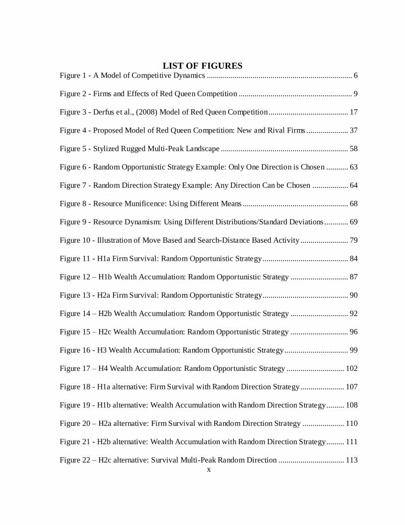
LIST OF FIGURES Figure 1 - A Model of Competitive Dynamics ......................................................................... 6
Figure 2 - Firms and Effects of Red Queen Competition ......................................................... 9
Figure 3 - Derfus et al., (2008) Model of Red Queen Competition ........................................ 17
Figure 4 - Proposed Model of Red Queen Competition: New and Rival Firms ..................... 37
Figure 5 - Stylized Rugged Multi-Peak Landscape ................................................................ 58
Figure 6 - Random Opportunistic Strategy Example: Only One Direction is Chosen ........... 63
Figure 7 - Random Direction Strategy Example: Any Direction Can be Chosen .................. 64
Figure 8 - Resource Munificence: Using Different Means ..................................................... 68
Figure 9 - Resource Dynamism: Using Different Distributions/Standard Deviations ............ 69
Figure 10 - Illustration of Move Based and Search-Distance Based Activity ........................ 79
Figure 11 - H1a Firm Survival: Random Opportunistic Strategy ........................................... 84
Figure 12 – H1b Wealth Accumulation: Random Opportunistic Strategy ............................. 87
Figure 13 - H2a Firm Survival: Random Opportunistic Strategy ........................................... 90
Figure 14 – H2b Wealth Accumulation: Random Opportunistic Strategy ............................. 92
Figure 15 – H2c Wealth Accumulation: Random Opportunistic Strategy ............................. 96
Figure 16 - H3 Wealth Accumulation: Random Opportunistic Strategy ................................ 99
Figure 17 – H4 Wealth Accumulation: Random Opportunistic Strategy ............................. 102
Figure 18 - H1a alternative: Firm Survival with Random Direction Strategy ...................... 107
Figure 19 - H1b alternative: Wealth Accumulation with Random Direction Strategy......... 108
Figure 20 – H2a alternative: Firm Survival with Random Direction Strategy ..................... 110
Figure 21 - H2b alternative: Wealth Accumulation with Random Direction Strategy......... 111
Figure 22 – H2c alternative: Survival Multi-Peak Random Direction ................................. 113

xi
Figure 23 – H3 alternative: Wealth Accumulation Using Random Direction ...................... 116
Figure 24 - H3 alternative: Firm Survival: Random Opportunistic ...................................... 117
Figure 25 - H3 alternative: Firm Survival with Random Direction ...................................... 117
Figure 26 – H4 alternative: Firm Survival Search-Distance Based ...................................... 118
Figure 27 – H4 alternative: Wealth Accumulation Move Based .......................................... 119
Figure 28 – H4 alternative: Firm Survival Move Based ....................................................... 120
xii
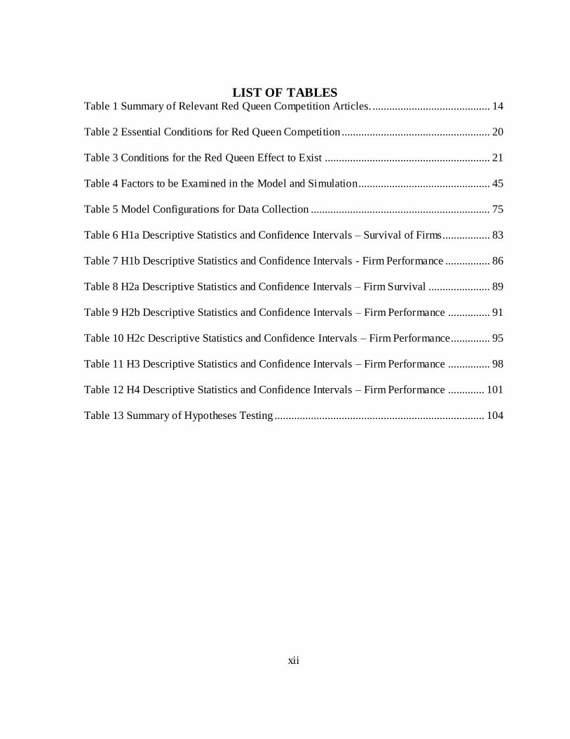
LIST OF TABLES Table 1 Summary of Relevant Red Queen Competition Articles. .......................................... 14
Table 2 Essential Conditions for Red Queen Competition ..................................................... 20
Table 3 Conditions for the Red Queen Effect to Exist ........................................................... 21
Table 4 Factors to be Examined in the Model and Simulation ............................................... 45
Table 5 Model Configurations for Data Collection ................................................................ 75
Table 6 H1a Descriptive Statistics and Confidence Intervals – Survival of Firms................. 83
Table 7 H1b Descriptive Statistics and Confidence Intervals - Firm Performance ................ 86
Table 8 H2a Descriptive Statistics and Confidence Intervals – Firm Survival ...................... 89
Table 9 H2b Descriptive Statistics and Confidence Intervals – Firm Performance ............... 91
Table 10 H2c Descriptive Statistics and Confidence Intervals – Firm Performance.............. 95
Table 11 H3 Descriptive Statistics and Confidence Intervals – Firm Performance ............... 98
Table 12 H4 Descriptive Statistics and Confidence Intervals – Firm Performance ............. 101
Table 13 Summary of Hypotheses Testing ........................................................................... 104
CHAPTER 1: INTRODUCTION A fundamental question in strategic management is, ―Why do some firms outperform
their rivals?‖ This is a particularly critical issue for new firms in technology industries (Shan,
Walker & Kogut, 1994; Zahra, 1996). Researchers to-date have presented several answers to the
general question of why firms vary in their competitive performance. One perspective is based
on an industry structure perspective that draws on competitive forces and barriers to entry and
mobility to place firms in favorable and unfavorable positions (Caves & Porter, 1977; Porter,
1980). A second perspective is suggested by Barney (1986) who uses a resource-based view to
depict ways that rival firms can be constrained when competitors acquire or create unique,
valuable, and rare resources that are difficult for the rivals to imitate. A third perspective comes
from evolutionary theory, which outlines how performance differences among rival firms are due
to a competitive race to gain an ultimate competitive advantage. This theory draws on the
advantages provided by superior speed and innovation by one firm to keep ahead of its rivals
(Nelson & Winter, 1982). The focus of my dissertation is based on a particular form of this third
perspective, one of the least-explored and understood regarding new firms, the Red Queen
Effect.
Red Queen competition, by definition (Barnett, 1997, 2008), is when one firm‘s actions
directly affect that firm‘s viability and also the viability of rival firms. Further, the actions taken
by the firm are escalated, in relationship to the rival firm, in terms of the rate of execution of the
actions. Barnett (1997) defined the components of this variance as the direct and indirect effects
of competitive actions on the focal firm (the primary firm under study) and rival firms (the
‗other‘ firms). The actions of the focal firm affect the performance of the focal firm, and these
actions also have an effect on the performance of rival firms. Red Queen competitive theory
2
focuses on these variances between rivals, and it is particularly well-suited for studying new
firms (Barnett, 1997) as they emerge and define their competitive strategy.
Competitiveness varies from organization to organization as shown by the wide range of
performance reported by companies worldwide in the stock market. The question regarding why
some firms outperform others can be further narrowed to, ―Why are some new firms more
competitive than their rivals?‖ New firms face a number of challenging issues surrounding the
liability of their newness (Stinchcombe, 1965). Many of these issues stem from resource scarcity
(Barney, 1991; Peteraf, 1993), the impact of environmental conditions (Hannan, 1998;
Henderson, 1999), founding team effects (Eisenhardt & Schoohnoven, 1990), the initial stocks of
financial and human capital (Cooper, Gimeno-Gascon, & Woo, 1994), the orientation of the
founding entrepreneur (Covin & Slevin, 1989), and the ethical climate of the new firm
(Neubaum, Mitchell, & Schminke, 2004). However, the findings of several studies indicate that
the results are mixed when it comes to theories about why firms struggle in their early years. In
particular, studies that have examined theories related to the liability of newness have found
cases of a genuine inverse relationship between age and death rates (Aldrich et al., 1989; Bruderl
& Schussler, 1990; Carroll & Huo, 1988; Singh, House, & Tucker, 1986; and Staber, 1989).
Using the research lens of Red Queen competition should provide insight into one important
source of this variance.
The focus of this dissertation is on new firms, and why some are more competitive than
others. One way to examine this question is to study how new firms deal with each of their
liabilities. One approach that is emerging in our domain of research is to examine the actions of
new firms one at a time in light of the strategies used by the firms. These are strategies that these
3
firms believe are the most suited to their industry, given the firm‘s goals and resources. The
strategy the firms choose is reflected in the actions that the firm uses to compete in its industry,
either to initiate a move or to react to a rival firm‘s move (Prahalad & Bettis, 1986). However,
researchers have paid limited attention to the discrete competitive actions of new firms with
regard to rival firms and the subsequent effect this has on the performance of these firms over
time. One reason for this is that competitive conditions are typically studied at an aggregate
level as they relate to markets, industries, or populations (Hannan & Freeman, 1989; Schere &
Ross, 1990; Tirole, 1988) under cross-sectional analysis. While this aggregate information is of
great interest on the one hand, on the other hand it may lack the fine-grained insight often needed
to address the mixed findings noted to-date.
Research that focuses on the series of actions or moves made by a first actor, and on
reactions or countermoves made by a responder in an industry, is competitive dynamics research
(Smith et al., 1991). The actions of individual firms in a market domain reflect that firm‘s
strategy as it finds positions to adapt to the competitive landscape and secure resources. This
coincides with the robust findings of research in the ecological evolution of firms (Kauffman,
1993). Red Queen competition, essentially a subset of competitive dynamics with a genesis in
evolutionary biology, is particularly well-suited to examine the discrete competitive actions
among new firms. Red Queen research is unique from general competitive dynamics research in
several ways. The first way is that it is limited to competitive activities that escalate among
firms. Without the escalation in the level of activities among firms, the competition is not Red
Queen by definition. Another way is that the firms must show evidence of adapting to either
4
their competition or their environment as part of their activity. A third way is that the rivalry
among the firms must impact the firm, and its rival, and the environment.
Research in this area is still emerging. Gaps in the research are already forming due to a
variety of approaches used to-date and analysis results that are not reliable as a result of data
collection and interpretation. One critical gap is the lack of an established model to examine Red
Queen competition and the Red Queen Effect. In order to address these gaps and to address
important issues within the literature, the purpose of this dissertation is to develop a model of
Red Queen competition for new rival firms. Using the model, I examine how, over time, the
basic tenants of Red Queen competition affect the survival and performance of rival firms. In
addition, I examine how the competitive environment affects the survival and performance of
firms engaged in Red Queen competition.
The remainder of this chapter proceeds as follows. First, I provide a broad and general
view of competitive dynamics. Second, I discuss the specific application of competitive
dynamics, Red Queen competition. From this discussion, in the third section, I identify the
necessary condition for Red Queen competition to exist. Using these conditions, I describe in
the fourth section the main relationships of interest in my study of Red Queen competition.
Finally, I review the relevant work studying Red Queen competition and the Red Queen Effect.
In general, during this literature review, I will highlight the significant relationships,
variables, and expected effects that are applicable to my current inquiry. In Chapter two I
explain my model of Red Queen competition and develop propositions and hypotheses to
correspond to the model. I provide the details for the simulation model and method that I use to
collect data and test these hypotheses. Chapter three details the results of the simulation data
5
used to test the hypotheses. Chapter four concludes with a general discussion of the findings
from the simulation, their practical and theoretical implications, and a discussion of potential
future research.
Literature Review
Typically the primary focus of strategic management theory is at the firm level and how
firm interaction with each other affects their competitive advantage. Therefore, my study is at
the firm level, and I examine how firms‘ actions among rival affects their survival and
performance. I also specifically focus on the actions of new firms in an environment that mimics
technology industries.
A well chosen and executed firm strategy is essential for a firm to adapt to the
competitive dynamics of its industry and realize its full competitive advantage (Porter, 1980,
1985). This is particularly true for new firms that are new and vulnerable (Stinchcombe, 1965).
Part of the challenge for new firms is they have fewer resources and less experience to draw
upon as they attempt to adapt to complex environments. Each action a new firm takes is usually
more costly, in a relative way, than a similar action by an existing rival firm.
One pattern of rivalrous firm action that is prominent in many industries is an escalation
of actions (Barnett, 1996). This escalation of actions is thought to either help a firm adapt to
rivals and to the environment as it learns from the actions, or in cases of maladaptation, it leads
the firm to enter a competency trap and often results in suboptimal performance by the firm. This
is one of the primary challenges faced by new firms – deciding what actions to take, when to
take them, and which firms to take action with. In addition to these competitive action decisions,
new firms deal with other critical factors. These factors include the evolving nature of their
competitors and the dynamics of the environment. Studies in the past that considered only a
6
cross-sectional, or static view of the competitive situation, may have missed important nuances
that in turn led to mixed findings in research results. Therefore, to address the dynamics of firm-
to-firm rivalry, I consider the use of the competitive dynamics research method. Examining the
competitive actions of both new firms and existing rival firms over a period of time should
provide me with the critical insight that perhaps has been missed in past cross-sectional and
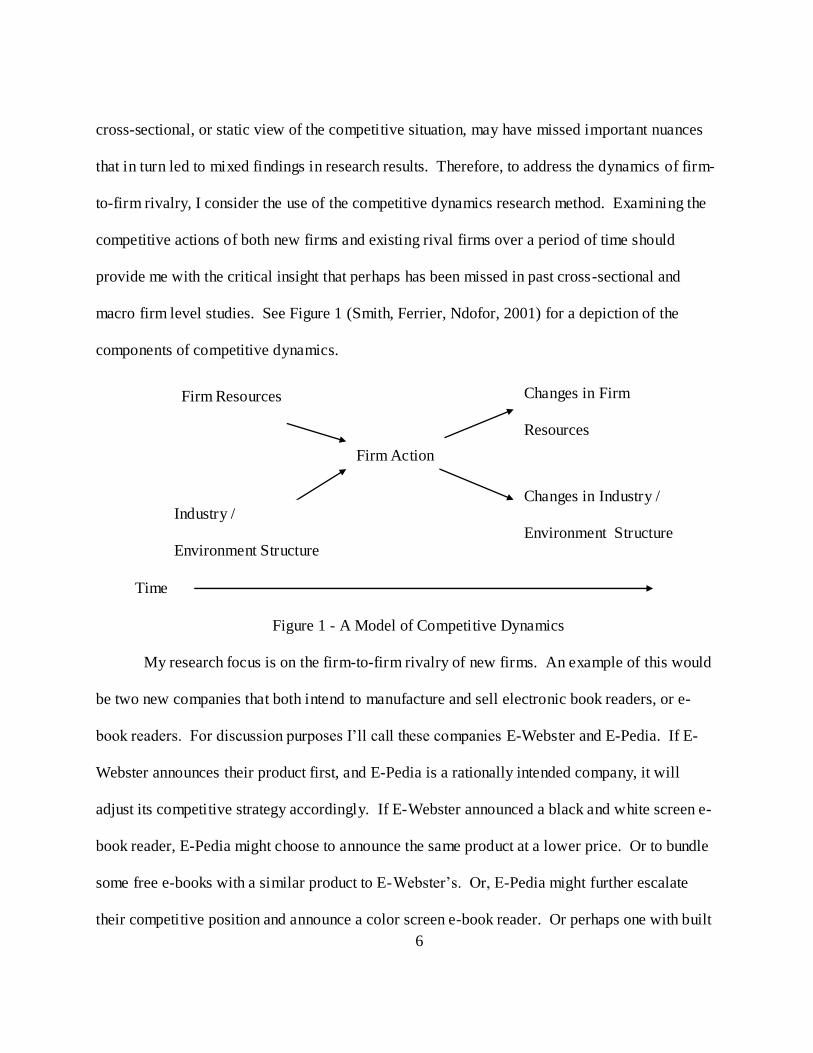
macro firm level studies. See Figure 1 (Smith, Ferrier, Ndofor, 2001) for a depiction of the
components of competitive dynamics.
Figure 1 - A Model of Competitive Dynamics
My research focus is on the firm-to-firm rivalry of new firms. An example of this would
be two new companies that both intend to manufacture and sell electronic book readers, or e-
book readers. For discussion purposes I‘ll call these companies E-Webster and E-Pedia. If E-
Webster announces their product first, and E-Pedia is a rationally intended company, it will
adjust its competitive strategy accordingly. If E-Webster announced a black and white screen e-
book reader, E-Pedia might choose to announce the same product at a lower price. Or to bundle
some free e-books with a similar product to E-Webster‘s. Or, E-Pedia might further escalate
their competitive position and announce a color screen e-book reader. Or perhaps one with built
Changes in Firm
Resources
Firm Resources
Firm Action
Changes in Industry /
Environment Structure
Industry /
Environment Structure
Time
7
in wireless communications, presuming E-Webster‘s did not have wireless. E-Webster might in
turn soon announce a larger sized color screen e-reader with a free subscription to the Wall Street
Journal. This is an example of two new firms that compete directly for the same type of
customer in the same market space and they match and exceed the competitive moves by
escalating their product offerings in response to the other firm‘s moves. This is Red Queen
competition, a specific form of competitive dynamics that examines the effect that competitive
rivalry has on the competing firms as they fight for survival and coevolve1 in an environment.
The term Red Queen competition, which may lead to the Red Queen Effect, is derived from the
discussion between the characters of the Red Queen and Alice in Lewis Carroll‘s Through the
Looking Glass2 (1865). Van Valen (1973), a biologist, used this analogy to describe the
nonstop, escalating activity and development that biological entities pursue as they try to
maintain and improve their fitness in a dynamic system. Since then, researchers have used the
concept to explain individual and firm actions in a variety of settings from biology to nuclear
escalation (Axelrod, 1997; Baumol, 2004).
The purpose of this literature review is to set the stage for a discussion of the Red Queen
Effect and specifically how to develop a model of the Effect. I use a model and simulations run
with the model to allow a controlled and precise way to examine some of the fundamental
assumptions that comprise the Red Queen Effect. Throughout the following review, I highlight
1 In my study, the term coevolve is limited to the concept of the mutual development of the firms
who are in a rivalrous competition. It is not intended to convey the fuller meaning of the
development of a species or a firm to the point that the firm gives birth to a new firm. 2 Alice was troubled by her lack of progress achieving her goals, and the Red Queen advised
Alice, ―Here, you see, it takes all the running you can do, to keep in the same place. If you want
to get somewhere else, you must run at least twice as fast as that!‖ (Carroll, 1960: 345).
8
important relationships that serve as a rationale for why and how I developed my simulation
model.
Theoretical Underpinnings of the Red Queen Effect
Competitive Dynamics and Red Queen Competition
Competitiveness varies from organization to organization as shown by the wide range of
performance reported by companies worldwide in the stock market. Using the research lens of
Red Queen competition should provide insight into one important source of this variance. Red
Queen competition, by definition (Barnet, 1997, 2008), is when one firm‘s actions directly affect
that firm‘s viability and also the viability of rival firms. Further, the actions taken by the firm are
escalated, in relationship to the rival firm, in terms of the rate of execution of the actions.
Barnett (1997) defined the components of this variance as the direct and indirect effects of
competitive actions on the focal firm (the primary firm under study) and rival firms (the ‗other‘
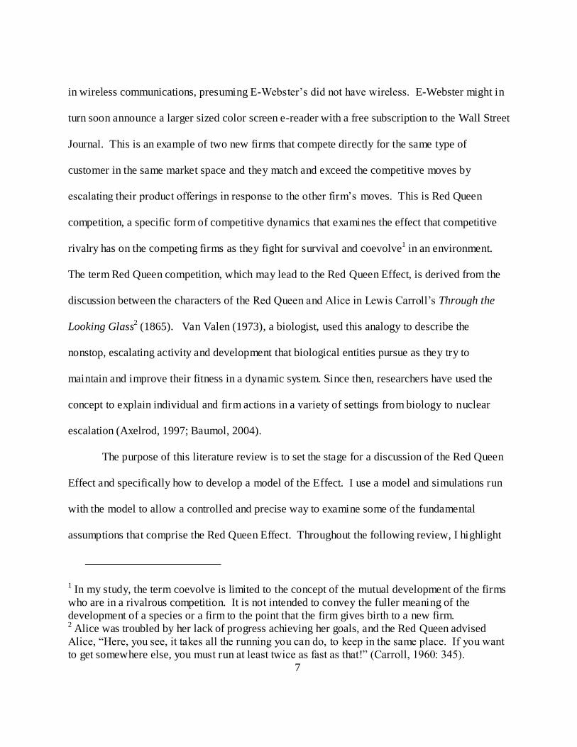
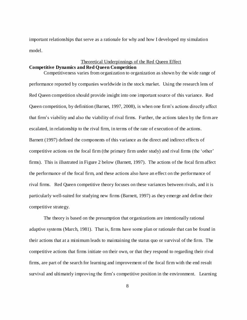
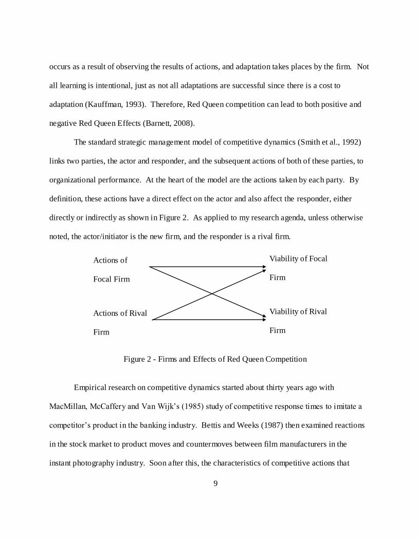
firms). This is illustrated in Figure 2 below (Barnett, 1997). The actions of the focal firm affect
the performance of the focal firm, and these actions also have an effect on the performance of
rival firms. Red Queen competitive theory focuses on these variances between rivals, and it is
particularly well-suited for studying new firms (Barnett, 1997) as they emerge and define their
competitive strategy.
The theory is based on the presumption that organizations are intentionally rational
adaptive systems (March, 1981). That is, firms have some plan or rationale that can be found in
their actions that at a minimum leads to maintaining the status quo or survival of the firm. The
competitive actions that firms initiate on their own, or that they respond to regarding their rival
firms, are part of the search for learning and improvement of the focal firm with the end result
survival and ultimately improving the firm‘s competitive position in the environment. Learning
9
occurs as a result of observing the results of actions, and adaptation takes places by the firm. Not
all learning is intentional, just as not all adaptations are successful since there is a cost to
adaptation (Kauffman, 1993). Therefore, Red Queen competition can lead to both positive and
negative Red Queen Effects (Barnett, 2008).
The standard strategic management model of competitive dynamics (Smith et al., 1992)
links two parties, the actor and responder, and the subsequent actions of both of these parties, to
organizational performance. At the heart of the model are the actions taken by each party. By
definition, these actions have a direct effect on the actor and also affect the responder, either
directly or indirectly as shown in Figure 2. As applied to my research agenda, unless otherwise
noted, the actor/initiator is the new firm, and the responder is a rival firm.
Figure 2 - Firms and Effects of Red Queen Competition
Empirical research on competitive dynamics started about thirty years ago with
MacMillan, McCaffery and Van Wijk‘s (1985) study of competitive response times to imitate a
competitor‘s product in the banking industry. Bettis and Weeks (1987) then examined reactions
in the stock market to product moves and countermoves between film manufacturers in the
instant photography industry. Soon after this, the characteristics of competitive actions that
Actions of
Focal Firm
Actions of Rival
Firm
Viability of Focal
Firm
Viability of Rival
Firm

10
triggered rapid responses of high technology firms were identified by Smith, Grimm, Chen, and
Gannon (1989). In addition to these industries of banking, photography, and high technology,
the industries of airlines, retailing, software, and telecommunications have also been examined.
Data for these studies spans field interviews, case studies, surveys, and archival sources.
Competitive dynamics does not focus on any one particular variable. Rather, the focus is on the
action between firms directly in the industry of interest. In this way, competitive dynamics
research is a natural outgrowth of Schumpeter‘s theory of creative destruction (Smith et al.,
1992). Schumpeter (1934) put forth the notion of creative destruction3 to outline the dynamic
market processes by which entrepreneurial firms act and react to exploit market opportunities.
The action of an entrepreneur in pursuit of new opportunities draws a reaction from incumbents
in a market domain. Should the entrepreneur‘s move prove advantageous, the delay in a
responder‘s countermove is what creates a momentary competitive advantage and higher-than-
normal profits ensue to the entrepreneur until the incumbent‘s reaction negates the advantage
(Nelson and Winter, 1982: Porter, 1980). Competitive dynamics research is focused on
identifying strategic actions that create these momentary competitive advantages. It follows then
that the use of competitive dynamics is appropriate for researching the strategic interactions used
by new firms as they seek to generate a competitive advantage relative to their rivals (Chen,
1988).
Competitive dynamics research is concerned with the interactions between firms in an
industry (Smith, Ferrier, & Ndofor, 2001) as they compete for strategic resources. Specifically,
3 Creative destruction is defined as the inevitable and eventual market decline of leading firms
through the process of competitive action and reaction (Schumpeter, 1934).

11
it is concerned with the actions and reactions among the firms as they vie for a superior
competitive position in the industry. The hoped for consequences of firm action are changes in
the firm‘s resources and / or changes in industry structure that improve the fit of the firm and
possibly create barriers for rival firms. Red Queen competition can be considered a special case
of competitive dynamics.
Relevant Red Queen Literature
Barnett and Hansen (1996) first applied the concept of the Red Queen to the analysis of
organizational failure. Barnett and Sorenson (2002) suggested that the Red Queen effect can be
found at the intersection of organizational learning and organizational ecology: competition
among organizations gives rise to internal organizational learning processes and learning
increases the strength of organizational competition. The authors suggest that competition and
learning reinforce one another as organizations develop, and this is what van Valen (1973)
referred to as the ‗Red Queen.‘ This definition of the Red Queen led to the development of the
concept of Red Queen competition and the Red Queen effect.
These effects are typically studied at the firm level. Although the effects are studied after
a period of aggregation, it is the accumulation of actions over time and the accumulated effect
that is at the heart of this research. The theoretical parallels with evolutionary biology are the
comparisons to how species evolve over time, and the actions they take to adapt to other species
and their environment. Van Valen (1973) coined the term Red Queen when he was observing
how rival species would compete for resources. Baumol (2004, p. 238) applied the concept to
economics and noted that in his contention,
12
―… the Red-Queen scenario describes one of the most powerful economic
mechanisms in economic development and in history.‖
The work of Baumol (2004) and van Valen (1973) gave rise to researchers referring to the
Red Queen Effect as ‗the arms race‘ or ‗escalation of competition‘ which underscores one of the
essential elements of the Red Queen Effect – escalation of competitive activity between two or
more firms. Barnett and Hansen (1996), Barnett and Pontikes (2005), and Barnett and Sorenson
(2002) were some of the first to apply the concept of the Red Queen to management research.
Barnett (2008) continues to be a pioneer in this line of research. His recent empirical results,
taken from studies of banking and computer manufacturing, suggest that the Red Queen Effect
has both a positive and a negative effect on competitive rivalry, firm survival, and firm
performance.
As noted above, empirical research in the Red Queen Effect is not new. Most of the early
work was concentrated in the efforts of just a few researchers. However, Red Queen Effect
research has been gaining momentum during the last five years with publications in top tier
journals. As an example, Derfus, Maggitti, Grimm, and Smith (2008) used the Red Queen Effect
to study competitive actions and firm performance across eleven different industries. They used
content analysis to analyze these industries over a multi-year period to generate their data. In
contrast, Barnett typically used econometric data taken from specific firms. It is difficult to
compare results among studies due to the lack of consistency in how variables were defined, how
relationships between rival firms were characterized, and how results were measured. For
instance, a careful read of the 2008 paper by Derfus et al., suggests that an imprecise Red Queen
competition model may have been used, and that a true Red Queen Effect was not established. I

13
believe this was a significant contributor to the mixed results found by the authors. In short,
although they labeled their research Red Queen Effect, it does not appear to conform to the same
rigor that Barnett applied in his work. This will be discussed in more detail later in this chapter.
I present a summary of relevant Red Queen Competition articles in Table 1.
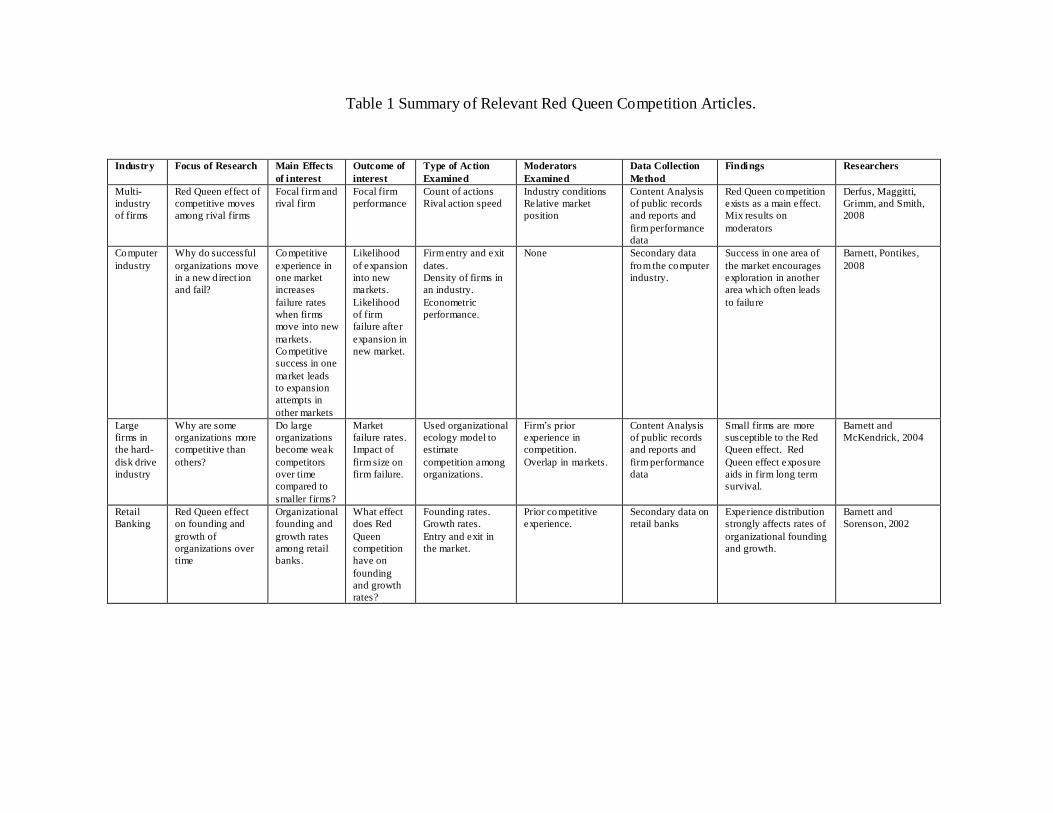
Table 1 Summary of Relevant Red Queen Competition Articles.
Industry Focus of Research Main Effects
of interest
Outcome of
interest
Type of Action
Examined
Moderators
Examined
Data Collection
Method
Findings Researchers
Multi-
industry
of firms
Red Queen effect of
competitive moves
among rival firms
Focal firm and
rival firm
Focal firm
performance
Count of actions
Rival action speed
Industry conditions
Relative market
position
Content Analysis
of public records
and reports and
firm performance
data
Red Queen competition
exists as a main effect.
Mix results on
moderators
Derfus, Maggitti,
Grimm, and Smith,
2008
Computer
industry
Why do successful
organizations move
in a new d irect ion
and fail?
Competitive
experience in
one market
increases
failure rates
when firms
move into new
markets.
Competitive
success in one
market leads
to expansion
attempts in
other markets
Likelihood
of expansion
into new
markets.
Likelihood
of firm
failure after
expansion in
new market.
Firm entry and exit
dates.
Density of firms in
an industry.
Econometric
performance.
None Secondary data
from the computer
industry.
Success in one area of
the market encourages
exploration in another
area which often leads
to failu re
Barnett, Pontikes,
2008
Large
firms in
the hard-
disk drive
industry
Why are some
organizations more
competitive than
others?
Do large
organizations
become weak
competitors
over time
compared to
smaller firms?
Market
failure rates.
Impact of
firm size on
firm failure.
Used organizational
ecology model to
estimate
competition among
organizations.
Firm‘s prior
experience in
competition.
Overlap in markets.
Content Analysis
of public records
and reports and
firm performance
data
Small firms are more
susceptible to the Red
Queen effect. Red
Queen effect exposure
aids in firm long term
survival.
Barnett and
McKendrick, 2004
Retail
Banking
Red Queen effect
on founding and
growth of
organizations over
time
Organizational
founding and
growth rates
among retail
banks.
What effect
does Red
Queen
competition
have on
founding
and growth
rates?
Founding rates.
Growth rates.
Entry and exit in
the market.
Prior competitive
experience.
Secondary data on
retail banks
Experience distribution
strongly affects rates of
organizational founding
and growth.
Barnett and
Sorenson, 2002
15
The Red Queen and New Firms
The concepts of firm action, and subsequent interactions with other firms, as depicted in
Figure 1 of competitive dynamics, meshes well with Red Queen competition as depicted in
Figure 2. Further, the action framework captured by Red Queen competition allows us to focus
on the execution part of the general theory of entrepreneurship (Shane, 2003). The model of the
entrepreneurship process suggests that the strategic actions of the new entrepreneurial firm are
revealed during the execution stage of the process. In the execution stage the firm assembles
resources, works out the organizational design of the firm, and begins to work out the strategic
posture of the firm. It is here that the firm decides how to compete with rival firms in the
marketplace (Porter, 1980). If the new firm chooses an escalating strategy of action it is
engaging in Red Queen competition.
The literature on interfirm competition emphasizes two conceptions of competition. The
first concentrates on the structure of markets and the other focuses on the conduct of individual
firms (Hannan & Freeman, 1989; Porter, 1980; Scherer & Ross, 1990). The separation of the
individual component and the environmental component of structure is consistent with the
general theory of entrepreneurship and competitive dynamics. In both views competition is an
action that is largely anonymous as firms compete for resources from a common pool.
Therefore, competition with existing unknown firms is one factor that new firms face. The other
related factor is direct rivalry with known firms. This difference was noted by Baum and Korn
(1996) in their research on competitive dynamics and interfirm rivalry. As these authors noted,
the essence of rivalry is a striving by firms in a market domain for potentially incompatible
positions (Caves, 1984; Scherer & Ross, 1990). Also, ―Firms feel the effects of each other‘s
16
moves and are prone to respond to them‖ (Porter, 1980: 88). This depiction mimics the
description of Red Queen competition – where two or more firms compete directly with each
other as they coevolve in a shared market domain. And finally, per Hannan and Freeman (1989:
140), this form of direct competition is what occurs when firms, directly identifiable to each
other, vie for the same resources in an environment characterized by limited resources.
Entrepreneurs create firms and enter the market domain to exploit an opportunity they
discovered. The new firm is instantly a rival if it enters a market domain with existing firms that
offer related products and sales taken by the new firm affect the potential sales of the rival firm.
The firm may have improved enough on a product to exploit a market opportunity that takes it
head-to-head with a known rival. However, if the firm has a breakthrough that leads to
exploration, it may enter the market with no direct rivals but still be competing for resources
from a common pool of firms. In summary, the Red Queen competition framework appears to
be well-suited to study ways in which new firms variance in actions leads to variance in their
performance over time.
The Strength and Weakness of Current Research – an Example
In one of the most comprehensive recent studies to-date on the Red Queen Effect, data are
compiled from content analysis, Derfus, Maggitti, Grimm, and Smith (2008) examined 11
different industries over a six year period. I will discuss this article in more detail since it is
recent and it one of the most comprehensive articles to-date. It represents both the strength and
weaknesses of current Red Queen competition research. The authors found full support for a
number of their hypotheses. These hypotheses dealt with how the rival actions of firms affected
their performance. The research concentrated on the number of rival actions and the speed of the

17
rival actions. Their research also investigated a variety of environmental or context moderators,
including firm level concentration (density), market demand, and market position of firms.
Typically no support or at the most very weak support was found for these moderators. The
Figure 3 illustrates theorized model from the Derfus et al., (2008) results:
Number of Focal Firm Actions Focal Firm
Performance
Rival actions and Rival
Speed of actions
Figure 3 - Derfus et al., (2008) Model of Red Queen Competition
Both focal and rival firm activity was measured by counting the number of actions attributed
to these firms using the process of content analysis4 for pricing, capacity, geographic changes,
marketing, and product introductions. Firm total actions, a key final measure used in the
analysis, were determined by summing all the counts of all the actions. While this is an efficient
way to collect data regarding the actions, it raises questions about the loss of information in the
final analysis. The aggregation of the types of actions by both focal and rival firms potentially
does away with Barnett‘s concept of competitive intensity. Also, no fine grained perspective is
maintained on the type of action analyzed, the impact of the actions.
4 Content analysis involves the examination of relevant published information about the firms‘
activities over a period of time, typically more text than numbers. The content is systematically
coded by defined variable type using a code book. The results are tabulated and analyzed as
secondary data.
18
In addition to my concern that all of the different types of actions are lumped together into
one generic aggregate action, only one side of the escalation question seems to be addressed – if
the focal firm increases actions, the rival firm increase. What about the reverse, when the rival
firm is the initiator? It is not clear that this side of the relationship is accounted for. Red Queen
competition stipulates that there is a two way interaction and this part of the relationship is not
addressed.
Further, all of the industry types are lumped together does away with the concept of specific
competitive context in Barnett‘s model of Red Queen competition. Although industry type is
controlled for in the regression analysis, this again is counter to one of the fundamental holdings
of Red Queen competition that firm types remain separated in the analysis of activity.
Finally, firm actions are collected and summarized on a yearly basis. This makes much of
the analysis time-based instead of activity-based. This may introduce an unwanted
normalization based on time versus highlighting concentrations of actions.
In summary, the research is interesting and according to the authors takes a step forward
toward addressing Red Queen Effect, but it does not seem to address the Red Queen Effect
directly. I suggest that Barnett might say that this is more of a competitive dynamics paper than
a true Red Queen paper. This is a significant point. I suggest that the requirements for Red
Queen competition were not explicitly met in this research. Rather, the requirements for
competitive dynamics were met instead. This leads me to the first major gap in Red Queen
competition research, the need to explicitly state the essential conditions for Red Queen
competition and the Red Queen Effect.
19
Essential Conditions for Red Queen Competition and Effect
Drawing from my literature review, I have outlined the essentials of Red Queen
Competition, the ones that are necessary before the Red Queen Effect can be considered. Many
of the published empirical studies that I examined do not meet these tests, although they liberally
refer to the Red Queen Effect. Note that these points are largely taken from Barnet‘s work (1997,
2008).
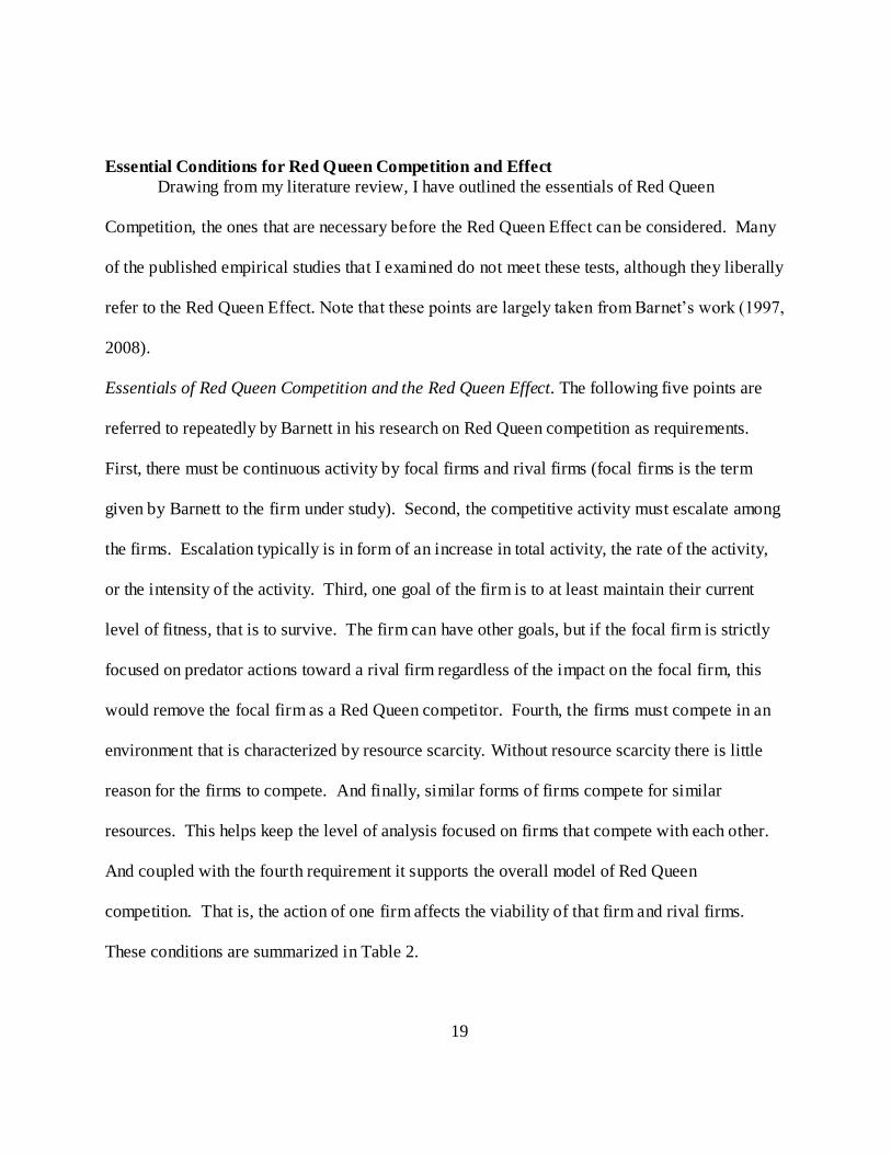
Essentials of Red Queen Competition and the Red Queen Effect. The following five points are
referred to repeatedly by Barnett in his research on Red Queen competition as requirements.
First, there must be continuous activity by focal firms and rival firms (focal firms is the term
given by Barnett to the firm under study). Second, the competitive activity must escalate among
the firms. Escalation typically is in form of an increase in total activity, the rate of the activity,
or the intensity of the activity. Third, one goal of the firm is to at least maintain their current
level of fitness, that is to survive. The firm can have other goals, but if the focal firm is strictly
focused on predator actions toward a rival firm regardless of the impact on the focal firm, this
would remove the focal firm as a Red Queen competitor. Fourth, the firms must compete in an
environment that is characterized by resource scarcity. Without resource scarcity there is little
reason for the firms to compete. And finally, similar forms of firms compete for similar
resources. This helps keep the level of analysis focused on firms that compete with each other.
And coupled with the fourth requirement it supports the overall model of Red Queen
competition. That is, the action of one firm affects the viability of that firm and rival firms.
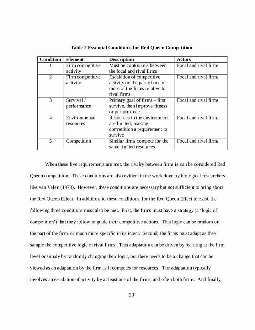
These conditions are summarized in Table 2.
20
Table 2 Essential Conditions for Red Queen Competition
Condition Element Description Actors
1 Firm competitive
activity
Must be continuous between
the focal and rival firms
Focal and rival firms
2 Firm competitive
activity
Escalation of competitive
activity on the part of one or
more of the firms relative to
rival firms
Focal and rival firms
3 Survival /
performance
Primary goal of firms – first
survive, then improve fitness
or performance
Focal and rival firms
4 Environmental
resources
Resources in the environment
are limited, making
competition a requirement to
survive
Focal and rival firms
5 Competition Similar firms compete for the
same limited resources
Focal and rival firms
When these five requirements are met, the rivalry between firms is can be considered Red
Queen competition. These conditions are also evident in the work done by biological researchers
like van Valen (1973). However, these conditions are necessary but not sufficient to bring about
the Red Queen Effect. In additions to these conditions, for the Red Queen Effect to exist, the
following three conditions must also be met. First, the firms must have a strategy (a ‗logic of
competition‘) that they follow to guide their competitive actions. This logic can be random on
the part of the firm, or much more specific in its intent. Second, the firms must adapt as they
sample the competitive logic of rival firms. This adaptation can be driven by learning at the firm
level or simply by randomly changing their logic, but there needs to be a change that can be
viewed as an adaptation by the firm as it competes for resources. The adaptation typically
involves an escalation of activity by at least one of the firms, and often both firms. And finally,
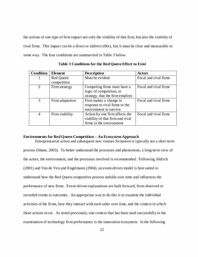
21
the actions of one type of firm impact not only the viability of that firm, but also the viability of
rival firms. This impact can be a direct or indirect effect, but it must be clear and measurable in
some way. The four conditions are summarized in Table 3 below.
Table 3 Conditions for the Red Queen Effect to Exist
Condition Element Description Actors
1 Red Queen
competition
Must be evident Focal and rival firms
2 Firm strategy Competing firms must have a
logic of competition, or
strategy, that the firm employs
Focal and rival firms
3 Firm adaptation Firm makes a change in
response to rival firms or the
environment to survive
Focal and rival firms
4 Firm viability Action by one firm affects the
viability of that firm and rival
firms in the environment
Focal and rival firms
Environments for Red Queen Competition – An Ecosystem Approach
Entrepreneurial action and subsequent new venture formation is typically not a short term
process (Shane, 2003). To better understand the processes and phenomena, a long-term view of
the actors, the environment, and the processes involved is recommended. Following Aldrich
(2001) and Van de Ven and Engelmann (2004), an event-driven model is best suited to
understand how the Red Queen competitive process unfolds over time and influences the
performance of new firms. Event-driven explanations are built forward, from observed or
recorded events to outcomes. An appropriate way to do this is to examine the individual
activities of the firms, how they interact with each other over time, and the context in which
these actions occur. As noted previously, one context that has been used successfully in the
examination of technology firm performance is the innovation ecosystem. In the following
22
section I set forth a definition of an innovation ecosystem and propose how this framework can
be used to study new firms engaged in Red Queen competition.
Scholars in entrepreneurial theory have called for the use of more holistic frameworks that
consider both the new firm and the firm‘s environmental context when conducting research on
these new firms (Shane, 2003). One framework that has emerged to address these issues is the
innovation ecosystem (Arned, 1996, 2010; Iansiti & Levien, 2004a, 2004b; Moore, 1993; Pierce,
2009). The innovation ecosystem is based on analogies drawn from evolutionary biology and it
provides descriptions of how strategic outcomes emerge as a result of firms‘ interactions in
industry environments. An innovation ecosystem framework is constructed to aid the study of
firm adaption in high technology industries. Following the biological concept of an ecosystem,
an innovation ecosystem suggests a multi-level view of firm adaptation and coevolution with
other firms and the environment, that is, individual firms and the market domain that represents
all of the firms. In conjunction with these levels, an ecosystem view is dynamic and takes a
longitudinal perspective. In addition, an innovation ecosystem includes the resource needs of the
firms and the stocks of these resources as part of the environmental conditions of the framework
(Moore, 1993).
The concept of applying a biological ecosystem to business in the form of a business
ecosystem owes its genesis to a merger of anthropological sciences and business theory. This is
a promising framework that incorporates prior work defining the general business ecosystem
(Moore, 1993, 1996), and then adapted it to focus on high technology industries that comprise an
innovation ecosystem. Moore put forth a broad reaching comparison of biological ecosystems
23
and business strategy in a business ecosystem model. The business ecosystem model was based
on the following definition from Moore (1996: 26), in which he defined a business ecosystem to
be:
―An economic community supported by a foundation of interacting organizations and
individuals—the organisms of the business world. This economic community produces
goods and services of value to customers, who are themselves members of the ecosystem.
The member organizations also include suppliers, lead producers, competitors, and other
stakeholders. Over time, they co-evolve their capabilities and roles, and tend to align
themselves with the directions set by one or more central companies. Those companies
holding leadership roles may change over time, but the function of ecosystem leader is
valued by the community because it enables members to move toward shared visions to
align their investments and to find mutually supportive roles.‖
Subsequent to Moore‘s work, Rothschild (2001) laid out the relationship between economics
and biological ecosystems in detail. The concept of an innovation ecosystem has grown in
importance for business research and practice as researchers have further developed the
integration of business strategy, economics, and ecology as a holistic analysis framework for
technology industries (Adner, 2006; Adner & Kapoor, 2010; Iasnsiti & Levien, 2004). The
innovation ecosystem view considers the new technology firm, and the entrepreneurial
environment as a coevolving system. The application of this framework by high technology
firms and enterprises is noted in reports from Cisco (Cisco, 2008), IBM (IBM, 2008), and MIT
(MIT, 2009).
24
New firms are like evolving species in an ecosystem. They typically are not able to fully
analyze the complex environments and calculate actions that lead to their optimal strategy and
eventually a position of competitive advantage. Firms that survive their environments do so by
learning to adapt their strategy over time-based upon what works or does not work for them (van
Valen, 1973). Therefore the initial choice of how to compete, and subsequent adaptations, are
keys to surviving and reaching positions of competitive advantage. This process of choice and
adaption is complex in technology industries, and the innovation ecosystem framework places
the coevolving firms in an environmental context.
The environmental factors that affect organizational performance in an innovation
ecosystem can be grouped into three categories (Sharman & Dean, 1991). The categories were
conceptualized through the research that spanned from March and Simon (1958) to Dess and
Beard (1984). These three categories are resource availability (the level of resources available to
firms in the environment), instability or dynamism (the rate of unpredictable environmental
change), and complexity (the level of complex knowledge that understanding the environme nt
requires). Sharman and Dean (1991) examined the research to-date and tested the predictive
validity of Dess and Beard‘s (1984) measurement of these constructs. Their results confirmed
the categories of the environmental measures, but they did revise the specific measurement
methods used by Dess and Beard for each of the categories to improve the predictability of
organizational performance. Further, they specifically identified the three categories as
dynamism, competitive threat, and complexity.
25
Dynamism consists of three components that identify the instability of the environment.
The three measures are: 1) instability in the value of shipments, 2) instability in the number of
employees, and 3) technological instability.
The competitive threat measure was revised and consists of four components that
measure munificence, concentration, or change in market conditions. The four components are:
1) value of shipments, 2) the number of employees, 3) the number of firms that comprise the top
market share holders, and 4) the average market share change of the top firms in the industry.
The revised complexity measure consists of four components. The four components are:
1) geographic concentration of firms, 2) the geographic concentration of the number of
employees, 3) the percentage of scientists and engineers as a total of all employee in an industry,
and 4) the number of seven digit SIC codes (the number of product categories) in the industry.
Note that all of the revised measures used Z scores to insure that all scale values were on the
same metric.
Research Questions Of Interest In Red Queen Competition
The literature I‘ve described shows the value of the Red Queen Effect in managerial
research. However, this research, and competitive dynamics research more broadly, are limited
in several ways. One limitation is the blurring of terms used to define Red Queen competition
and the Red Queen Effect. Another limitation is the mixed results of early research findings.
My review leads me to believe that a study that first defines the fundamentals of Red Queen
competition, and sets this forth in a theoretical model, would be a valuable contribution to the
emerging Red Queen Effect and competitive dynamics literature. Thus, I will pursue the
following research questions using a design that defines the fundamentals, develops a theoretical

26
model from these fundamentals, and results in a simulation that allows for data collection to test
the model to addresses some of the limitations I‘ve noted in prior research.
My investigation will be guided by the following areas of interest and three general
research questions. Barnett (1989, 1997, 2008) found that Red Queen competition served to both
strengthen and weaken existing firms. Firms that engage in Red Queen competition at an
appropriate level may be strengthened by the competition (Barnett, 2008). However, firms that
engage in competitive action may fall into a competency trap that leads to maladaptive learning
and as a result, the firms experience a decline in performance (March, 1991; Kauffman, 1995).
This leads me to ask:
Research Question 1: How does Red Queen competition help explain the variance in new
firm survival and performance?
Also, Kauffman (1993) asserted that Red Queen competition is most promising when
firm behavior is balanced at the intersection of competitive chaos and stability, an abstract
location he termed ‗the edge of chaos.‘ This leads to questions about the equality of Red Queen
competitive actions. Can there be too much Red Queen competition? And if there is a tipping
point, or threshold, is it due to the number of actions, the speed of actions, the type of actions, or
some combination of these characteristics? This line of inquiry can be asked by:
Research Question 2: What are the effects of the various types and timing characteristics
of firm actions that comprise Red Queen competition on new firm performance?
By definition, firms in the same market domain compete for the same resources with rival
firms. In ecological competition this is a zero sum game, and resource scarcity severely
27
increases the competition (Moore, 1996). In a similar way, environmental conditions should
make a difference in how Red Queen competition affects new firm performance, and particularly
in industries with an innovation focus. This leads me to ask:
Research Question 3: How does the environmental context, specifically innovation
ecosystem factors of munificence and dynamism, moderate the effects of Red Queen
competition on new firm performance?
To address these research questions, I use an agent-based simulation of Red Queen
competition between new firms and rival firms. A properly designed model and simulation is an
effective way to develop and test theory (Davis, Eisenhardt, Bingham, 2007). Agent-based
models enhance our capacity to model competitive and cooperative behaviors at both the firm
and the environment level of analysis (Elliot & Keil, 2002). To my knowledge this is the first
study to explore Red Queen competition using an adaptive agent-based simulation.
28
CHAPTER 2: RED QUEEN COMPETITION SUGGESTED MODEL AND RESEARCH HYPOTHESES
Suggested Course For Model And Simulation Development
Prior research on Red Queen competition and the Red Queen Effect has shown promise and
has in turn encouraged additional research in this area. The bulk of the research was initiated by
Barnett, spanning the last twenty years. Barnett concentrated on the financial and computer
industries using an econometric approach. On the one hand, Barnett‘s definitions of what
constitutes Red Queen competition have evolved over time to represent our clearest picture yet
of this phenomenon. On the other hand, as the popularity of this research stream has increased,
so has the potential for blurring many of the key terms used in Red Queen competition and
accuracy of measurement criteria needed for precise research.
The development of a Red Queen competition model that accurately represents the essentials
of this form of competition can be used as a research tool for management studies to address
these concerns. To my knowledge, no such model has been developed for the business
management domain of research. The value of the model is multifold (Jacobides &Winter,
2010). First, modeling allows us to be honest when different terms are used in our literature.
This is one problem with the emerging stream of literature as I noted. Second, the process of
developing a model pushes our logic more than using only our intuition, and this in turn leads to
more precise definitions of measures and relationships. Also, once a theoretical model is
developed it is much easier to examine variations in the theory.
The first step in developing an accurate theoretical model requires that the essential
components and theoretical relationships of Red Queen competition be objectively defined.
29
They must be defined with sufficient precision so that they can be clearly, and hopefully
unambiguously, implemented in the model. Second, a model allows the researcher to manipulate
just the variables that are in question to test the hypotheses under examination while keeping
strict controls on the remaining variables. This approach should provide more insight into
causality than a cross-sectional survey or a longitudinal study using secondary or proxy data.
My experiences with this part of the research for my dissertation confirmed these points.
One of the identifying signatures of the Red Queen Effect is a pattern of reciprocity
between a focal firm (the firm under study) and a rival firm that typically escalates over time.
The escalation is denoted by an increase in the number of actions, or the rate the actions occur, or
the duration of the actions, and so forth. It is the dynamics of the actions and the resulting
adaptations by one or more of the firms that describes the competitive dynamics between the
firms. Therefore, the theoretical model must model these complex adaptive systems and do so at
the behavior level of both of the competing firms.
The implementation of a model requires explicit definitions for all of the model
components. This includes the variables, the relationship between the variables, the anticipated
outcomes as the variables interact, and precisely how all of these are measured. It is in this
specificity that we can gain ground on moving theory ahead. The first step is to establish a basic
model. Davis, Eisenhardt, and Bingham (2007) identified that the development of a theory
model and subsequent simulation is now regarded as an essential tool for theory development
and refinement in our domain. One reason is the completion of a basic model also provides a
foundation for the development of richer models. It follows that this would provide a means to
30
guide empirically based research in a manner more consistent with the essentials of Red Queen
competition. To accomplish these goals, the proposed model needs to be based on the essentials
of Red Queen competition, and it should be capable of generating identifiable Red Queen effects.
The focus of the model is how activity, particularly escalation of activity, between rival firms
affects both firms‘ survival and performance. Per van Valen (1973) there are three fundamental
components that must be present before Red Queen competition exists. These three components
are: continuous activity between rivals, escalating activity between rivals, and a minimum goal
of maintaining the current level of fitness for the firms involved.
I presented the essentials for Red Queen competition in Chapter One. In this chapter I
expand upon these essential, drawing primarily from the work of Barnett who has generated a
significant portion of the published research on Red Queen Effect in the management domain.
He is one of the early and sustained researchers, publishing from 1997 to 2008. He noted that
competitiveness varies from organization to organization, and Red Queen competition explains
many of the reasons why it varies and how it varies. For instance, Red Queen competition
requires that the characteristics of an organization j involved in competition with a rival i affects
not only the viability of j but also i. The same is said for rival i relative to organization j. That
is, both firms‘ characteristics affect their own viability as well as other firms‘ viability. Further,
organizations are intendedly rational, adaptive systems and therefore they keep searching until
they find the resources needed to survive. After survival, they search for an improvement in
performance. This adaptation, which can lead to both negative and positive outcomes, occurs
31
through organization learning, and simply through random behavior, or luck on the part of the
firms.
One environmental condition for Red Queen competition is that organization environments
must characterized by resource scarcity. Therefore, similar forms of organizations compete over
similar resources. In this way, rivalry matters, and more precisely, the competitiveness of the
rivalry matters. Superior organizational performance requires that an organization perform better
than its rivals according to the context‘s logic of competition, where logic of competition is
defined as ‗a system of principles in a given context that determines who can compete, how they
compete, on what criteria they succeed or fail, and what are the consequences of success or
failure.‘ Organizations learn a context‘s (environment‘s) logic of competition by competing.
Therefore, finding the best competitive logic for a context can be thought of as a sampling
problem where the problem is the environment, and one‘s rival. Therefore, organizational
adaptation should be modeled as a function of the competitive activity of an organization, not as
a function of elapsed time. This is one key differentiator in Red Queen research, that activity is
the principle unit of measurement, not time. For example, each time a firm is involved in a
competitive action is an event in Red Queen competition. If a firm is involved in five events in
one day, this is treated as five separate events. If a firm is involved in one event a week for five
separate weeks, this is treated as five separate events. On the other hand, some research is time-
based, and either records the number of events in a day or in a week and aggregates them
together as a factor of the elapsed time. Red Queen competition is concerned with activity
escalation and therefore must be activity-based.
32
From this discussion, I suggest that there are two main points to be considered when
modeling Red Queen competition. The first is that each firm must have a ‗logic of competition,‘
or what is more generally referred to as a firm‘s strategy. This logic should vary across contexts
(context based on technology, organizational structure, the industry, social and political factors,
etc.). Second, organizations sample their context‘s (environment‘s) logic of competition by
competing (considerable uncertainty surrounds the logic of competition in any given context –
sampling through competition allows the organization to learn and reduce uncertainty).
Therefore, my model will be based on two factors, a firm‘s logic of competition or its strategy,
and the environment that the firms compete in.
Firm Behavior. The model will feature variations in firm activity to allow me to examine the
way these activity variations affect firm survival and performance. Two firm types will be used.
For sake of clarity in the discussion and interpretation from this point on, the ‗focal‘ firm or the
‗new‘ firm will be referred to as the ‗Red Queen‘ firm. The ‗rival‘ firm will remain as the ‗rival‘
firm. Each firm type will have a clear logic of competition, or strategy, that the firm uses to
achieve the goal of sustaining or improving its performance.
As noted earlier, Red Queen competition is measured in terms of activity, not time.
Empirical studies to-date have predominately used rate of activity and type of activity. Effective
modeling is based on using the most basic and simple form of firm behavior (Derfus, et al., 2008;
March, 1991). After I engaged in detailed discussions with researchers5 in the field of
5 Dr. Ivan Garibay, a computational evolutionist, with the Center of Research and
Commercialization, University of Central Florida; Dr. William Rand of Maryland, Assistant
33
computational modeling and studying Red Queen models from the biological sciences, I believe
that two forms of activity are required to effectively model Red Queen competition: the rate of
firm moves, and the distance searched in a single move. Rate of firm moves can be represented
by the ratio of Red Queen firm moves to rival firm moves during the same activity window. A
ratio of 1 to 1, or simply 1, indicates that the Red Queen firm and the rival firm moved the same
amount. A ratio of 2 means the Red Queen firm moved at an escalated rate of twice that of the
rival firm. By the same process, distance searched, or what I term search-distance, can be
represented by the ratio of Red Queen distance ‗jumped‘ or ‗leaped‘ on the landscape to rival
firm distance ‗jumped‘ or ‗leaped‘ on the landscape during the same activity window. The key is
that when the ratio exceeds 1, then an escalation has occurred and Red Queen competition is in
effect.
The logic of competition needs to reflect the intended rationality of the firm. At a minimum
the firm needs to seek sufficient resources to survive. Beyond this mode of just surviving, the
firm seeks resources to achieve superior performance relative to other firms. Presuming for a
moment that the firms compete for resources on a common landscape, the firms need to move
around on the landscape to find the resources necessary for survival. One way that new firms
move is naively due to their newness to the industry. This type of movement is seemingly
random, in which all directions are considered of equal risk and value and therefore any direction
is acceptable. Firms with more knowledgeable or experienced management, even if new, show
Professor of Marketing and Research Director, Center for Complexity in Business, University of
Maryland. Dr. Andrew Nevai, Assistant Professor of Mathematics, University of Central Florida;
Dr. Betsy von Holle, Assistant Professor of Biology, University of Central Florida.
34
more consideration before they move. These firms choose a direction ahead of the firm taking
action and moving.
To keep the model focused, following the guidelines put forth by Davis, et al., (2007), I don‘t
explore direct firm-to-firm predation type of competition between Red Queen and rival firms that
lead to direct elimination, mergers, or acquisitions. These outcomes are feasible outcomes of
Red Queen competition, but they are beyond the scope of this research study.
When a firm takes action, it involves the expenditure of resources. Therefore firm actions
should not be costless in a model. An appropriate cost for both the type of action taken and the
amount of the action taken should be considered.
Environment. This study focuses on the behavior of new firms in a high technology
environment. These environments are typified as complex in nature (Kauffman, 1997). As
noted earlier, this study will use a landscape for the environment that firms compete on.
Environmental complexity, when modeled on landscapes, is modeled as a ‗rugged multi-peak‘
surface (Kauffman, 1997). The landscape represents the arena of competition that firms travel
across as they search for resources. Landscapes for agent-based models are represented as grids
with unique locations defined as squares on the grid. A rugged multi-peak landscape is created
with a variety of peaks that are all of different heights on the grid. The height of each unique
square on the grid will represent the resources available on that square. A three-dimensional
model of a rugged multi-peak might look like a Rocky Mountain landscape.
Resources are required for firm survival. Per Kauffman‘s fitness landscape definition,
resources that are represented on a landscape can be considered uniform resources in that they
35
represent whatever a firm needs at any particular time. They are allocated to specific locations
on the landscape, and they are consumed when a firm arrives at that location.
Resource replenishment is another important component of landscape models. Resource
replenishment needs to model the environment that is under study, in this case high technology
industries. I suggest that there are two essential components of resource replenishment. The
first is the rate of replenishment after resources are depleted at a location. The second is the total
amount of resources replenished at a particular location. Replenishment should be accomplished
in the most straightforward manner possible while representing the context being studied. Given
the nature of high technology environments resources are consumed and replenished rapidly.
Applied to a business context the Red Queen Effect is often positioned as a condition in
which each of the rival firm‘s performance depends on the firm‘s matching or exceeding the
actions of rivals (Derfus, Maggitti, Grimm & Smith, 2008). In these models performance
increases gained by one firm tend to lead to a decrease in performance in other firms. The only
way rival firms in such competitive races can maintain their performance relative to others is by
taking action of their own. Each firm is forced by others in an industry to participate in
continuous and escalating actions and development that are such that all the firms end up racing
as fast as they can just to stand still relative to competitors.
In summary, for the Red Queen Effect to be realized, the following essentials must be
satisfied by the model. First, firms should have a logic that they follow to guide their
competitive actions. This logic can be random or specific. Second, firms adapt as they sample
the competitive logic of rival firms. This adaptation can be driven by learning, or simply by
36
randomly changing their logic, but there needs to be a change that can be viewed as an
adaptation. Third, the actions of one type of firm impacts not only the viability of that firm, but
also the viability of rival firms. This concludes the summary of the basics of the theory model,
and how the model will support the essentials of Red Queen competition and Red Queen Effect.
Specific Relationships To Be Explored
Figure 4 identifies that the anticipated main effects are related to the actions of new firms and
their rival firms, both directly and as an interaction. Further, as shown in the figure, it is
anticipated that these effects are influenced, as a type of moderation, by the resource conditions
in the ecosystem.

37
Figure 4 - Proposed Model of Red Queen Competition: New and Rival Firms
As noted in my specific research model of Red Queen competition of new firms
presented above, three areas of research will be pursued. The first area is the relative speed of
adaptation and learning of the new firms. This area addresses research questions about the limits
of Red Queen competition, in new firms, per Kauffman‘s ―edge of chaos‖ (Kauffman, 1995) and
March‘s speed of learning (March, 1991). The second area focuses on the type of adaptive
action made by the new firms, in terms of search distance for resources, relative to existing
New Rival Firm Actions:
Speed/Rate of action
Distance searched
New Firm Actions:
Speed/Rate of action
Distance searched
New Firm Performance
Rival Firm Performance
Survival of the Firms
Environmental Conditions:
Dynamism (variance of
resource availability)
Munificence (mean or peak of
resource availability)
38
firm‘s location. This area addresses competency traps as suggested by March (1991) as
organizations make critical resource allocation decisions as they try to balance incremental and
significant learning steps. The third area considers the effects of the ecosystem on resources
needed for survival and possible performance advantages (Dess & Beard, 1984).
New firm action – fast/slow rate of adaptation. Most definitions of competitive advantage
(Porter, 1980, 1985) refer in some way to the value a firm carves out of the existing market, or
creates in a new market, and subsequently offers to customers in such a way that customers are
more attracted to this firm than to another firm offering similar products or services. Achieving
a competitive advantage for a firm is keenly dependent on the relative position of that firm to its
competition (Porter, 1988). In an innovation ecosystem, a significant portion of a firm‘s value
comes from the knowledge the firm gathers and puts to use (Moore, 1996, 2006) to gain an
advantage over its rivals. However, such advantage does not come immediately – it is an
iterative search and adaptation process (Kauffman, 1993), and for the entrepreneurial firm in a
technology industry it is more complex and subject to higher risks than established firms face
(McMullen & Shepherd, 2006).
It follows that this iterative adaptive process employed by new firms is highly dependent
on how the firm competes for information as it learns to adapt. Kauffman (1993, 1995) noted
that the degree of adaptation of a species is more a factor of the number of iterations of
adaptation that the species is exposed to than the passage of time. Therefore, it seems logical
that a key factor in new firm adaptation is the speed with which the firms take action. Note that
this is a measure of the rate of actions in a given period of time, not the response time after a

39
rival firm has acted, which is a measure of responsiveness. In this sense, speed of actions is best
described by a measure of the rate of actions in which rate is determined by summing all actions
in a given period of time and dividing this sum by the time in the period to obtain rate of action
per time. Each firm‘s rate is compared to other new firms, thereby creating the differential for a
fast adapting firm versus a slow adapting firm (March 1991). March found that fast individual
learning tends to have a favorable first-order effect on individual knowledge but an adverse
second-order effect on organizational knowledge.
Kauffman (1993) also found that Red Queen competition has a negative side to it. The
effort firms exert through their actions to compete, learn, and adapt has a cost to it. When
actions escalate such that the cost outweighs the benefits, the firm approaches what Kauffman
termed ―the edge of chaos‖ and firm performance declines. Also, the second-order effect of
March‘s (1991) slow and fast learning could also negatively affect the performance of the
ecosystem, which in turn affects the new firms. It follows that once a firm reaches the edge of
chaos, or pursues too high a rate of adaptation, that new firms that were performing relatively
better than other firms would experience a decline such that:
Hypothesis 1a: A new firm engaged in a higher rate of competitive moves for resources in
their environment, relative to a rival firm’s rate of moves, will initially have a greater survival
rate than the rival firm. This greater survival rate will peak and then decline as the competitive
action rate undertaken by the new firm continues to escalate relative to the rival firm.
Hypothesis 1b: A new firm engaged in a faster rate of competitive moves for resources in
their environment, relative to a rival firm’s rate of moves, will initially have a higher
40
performance than the rival firm. This higher performance will peak and then decline as the
competitive action rate undertaken by the new firm continues to escalate relative to the rival
firm.
New firm actions – local search and distant search adaptation. New firms are presumed to
be intentionally rational in their search patterns (Kauffman, 1993). Following the theory of
rational search (Simon, 1956), firms therefore should seek to balance their search efforts and
investment opportunities between exploration and exploitation. Exploration includes activities
described by terms such as novel, unique, wide-search, variation, high risk taking,
experimentation, discovery, and innovation. Exploitation includes terms such as refinement,
choice, efficiency, selection, imitation, and execution. Maintaining an appropriate balance
between exploration and exploitation is a primary factor in a firm‘s survival and prosperity.
However, it is unlikely that all new firms have the same limits of rationality, the same aspiration
levels, and the same drive to perform.
In complex technology industries like biotechnology, interactions between individuals
both within and between firms provide key resources in the form of knowledge and problem
solving through which innovations are created in organizations (Ahuja, 2000). Innovations are
built from knowledge creation, and knowledge creation is the product of learning processes. One
way learning is facilitated is by knowledge transfer between individuals as they interact, and in
the knowledge-based theory of the firm, organizations are recognized as social communities of
collected individuals specializing in efficient knowledge creation facilitated by knowledge
transfer (Kogut and Zander, 1996). Firms that intentionally or serendipitously facilitate the
41
transfer of knowledge in terms of time and effort are more likely to insure that transfers take
place efficiently and that they are successful (Hansen, 1999). Increases in knowledge
complexity places additional burdens on the firm to facilitate the transfer, and the type and
frequency of interactions may impact firm innovation performance.
March (1991) and Robson (2005) recognized this and concluded that firms in complex
industries that engaged primarily in activities focused on exploration to the exclusion of
exploitation are likely to find that they are very inefficient and inconsistent in product and
service development – they don‘t adapt well to immediate needs of their environment. On the
other hand, firms that engage in exploitation to the exclusion of exploration may find themselves
in a competency trap – a suboptimal stable equilibrium, per March (March, 1991). Given these
findings, it is reasonable to draw the conclusion that not all actions taken by new firms have
equal effect on the firms. And, that if we classify the actions under the categories of exploitation
or exploration, that we can examine the limits of Red Queen competition as it relates to these
classifications. Following March (1991) and related researchers, I suggest that:
Hypothesis 2a: A new firm engaged in a greater search-distance (with respect to the firm’s
current location) for resources relative to a rival firm with a smaller search-distance
(searches more locally) will initially have a greater survival rate than the rival firm. This
greater survival rate will peak and then decline as the search-distance undertaken by the new
firm continues to escalate relative to the rival firm search distance.
Hypothesis 2b: A new firm engaged in a greater search-distance (with respect to the firm’s
current location) for resources relative to a rival firm with a smaller search-distance
42
(searches more locally) will initially have a higher performance than the rival firm. This
higher performance will peak and then decline as the search-distance undertaken by the new
firm continues to escalate relative to the rival firm search distance.
And further, if given populations that represent similar conditions to satisfy ―all things being
equal‖ to provide for controls to isolate the actions under examination, I expect the following to
hold:
Hypothesis 2c: A new firm engaged in a more heterogeneous search-distance activity (that is
using a balanced mixture of local and distant search-distances) for resources will have a
higher performance than the rival firm that searches just more locally or just more distantly
for resources than the new firm.
Ecosystem environmental effects on red queen competition and firm performance. Beyond
variance in firm actions, we need to also consider how the conditions of the ecosystem affect
these actions. These external conditions should be observed over time to capture significant
variance as a possible source of explaining variance in firm performance. However, to my
knowledge, there is very limited research that has examined new firm competitive dynamics over
time as they relate to the Red Queen Effect under varying innovation ecosystem conditions.
New technology firms in innovation industries tend to evolve rapidly as they adapt or
they are typically selected out through direct attrition or acquisition. As firms adapt they may
choose to change their interaction strategy, or the characteristics of that strategy, and therefore
the strategies should be studied over time to capture the dynamics. This follows the evolutionary
processes of variation, selection, and retention (VSR) (Campbell, 1969, 1994). Firms invest
43
differently in the amount of variation, selection, or retention actions they conduct, which results
in varied patterns of adaptation and performance (Burgelman, 1994; Madsen & McKelvey,
1996). The ecosystem environment also plays a role in VSR. Evolutionary processes span
multiple levels of analysis (intrafirm, industry, and ecosystem) nested in a hierarchy (Aldrich,
1979). For instance, to sustain performance in a turbulent environment, firms may change their
experience-based knowledge by adopting new strategies (Hannan & Freeman, 1977),
competencies (McKelvey, 1982), or routines (Nelson & Winter, 1982) and diffusing, through
retention, these variations throughout the firm.
For new firms to remain viable they must learn and adapt to their environment. Severe
maladaptation can lead to a firm‘s elimination from the ecosystem. Superior adaptation leads to
competitive advantage in innovation ecosystems. Adaptation requires new firms to harness the
appropriate resources and successfully apply them to reach a unique position of value in the
ecosystem. Technology ecosystems by definition are complex and obtaining the right resources
and allocating them to insure that the firm learns what it needs to learn is complicated.
Considering the environmental condition of munificence, or resource availability
(Barnett, 1997, 2008; Barney, 1986, 1997; Peteraf & Bergen, 2003), when resources are scare in
the ecosystem, firms will need to compete even more aggressively for resources. Firms that
engage in Red Queen competition, that is higher levels of firm rivalry, should experience higher
levels of performance. Therefore, I suggest that:
Hypothesis 3: Environmental munificence (the average of resources available to firms in the
environment) will moderate the relationship between new firm competitive moves and rival
44
firm moves such that under conditions of low munificence a new firm that engage in Red
Queen competition (escalated rate of move) will have higher performance than a rival firm
that does not.
In essence, while munificence address the resources in the ecosystem, dynamism and
complexity reflect the degree of uncertainty facing firms in the ecosystem (Ferrier, Smith, &
Grimm, 1999; Lumpkin & Dess, 2001; Schumpeter, 1934, 1950). Lumpkin and Dess (2001)
found that proactiveness was positively associated with firm performance under conditions of
high dynamism. Proactiveness is associated with opportunity-seeking behavior and exploration
(March, 1991). It follows that firms using distant search actions are more likely to be successful
in changing and uncertain environments where the costs and risks of novelty are more likely
rewarded than in stable and predictable markets. Therefore, I suggest that:
Hypotheses 4: Environmental dynamism (the variance of resources available to firms in
the environment) will moderate the relationship between firm’s search for resources such
that under conditions of high dynamism (high variability), new firms that engage in Red
Queen competition (escalated distance searched) will have better performance than new
rival firms that do not.
Summary - Integrating The Essentials Into The Simulation Model
To integrate the essentials noted in this chapter into my simulation to support the collection
of data to test my hypotheses requires the development of a model with individual firms with
different logics of competition, or strategies. The model must allow for an escalation or
difference in the activity level among the types of firms. The actions of one type of firm must
impact that type of firm‘s performance and also the performance of rival firms. And finally, the
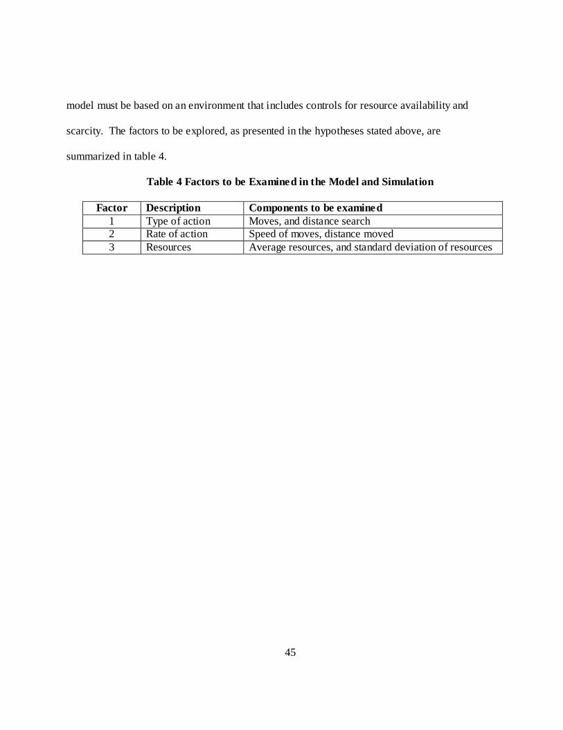
45
model must be based on an environment that includes controls for resource availability and
scarcity. The factors to be explored, as presented in the hypotheses stated above, are
summarized in table 4.
Table 4 Factors to be Examined in the Model and Simulation
Factor Description Components to be examined
1 Type of action Moves, and distance search
2 Rate of action Speed of moves, distance moved
3 Resources Average resources, and standard deviation of resources
46
CHAPTER 3: METHODS AND RESULTS From the onset of this research I followed the guidelines suggested by the Davis et al., (2007)
article on using simulation as a tool for the development and testing of theory. As noted by these
authors (p. 480):
―Simulation is an increasingly significant methodological approach to theory
development in the literature focused on strategy and organizations.‖
Red Queen competition is considered a complex adaptive system (Kauffman, 1993). In cases
involving Red Queen competition, where complex relationships among constructs exists, and in
particular when empirical results have limitations, simulation can provide better insight into the
relationships (Zott, 2003). One standout example is the work of March (1991) on organizational
learning. March used a matrix to model the code of the organization, and stochastic simulation
to examine the affects of slow and fast learning, as well as exploration and exploitation on
organizational learning. The fact that no empirical data were used in this influential research is
perhaps lost on first-time, and possibly even second-time, readers of this article.
On the other hand, as noted by Davis et al. (2007), some simulation methods often yield
very little in terms of actual theory development or clarification. These methods are typified by
models that are overly simplified to the point that they are based on unrealistic assumptions like
zero search costs (Rivkin, 2000), or all of the logic of competition rules are equally effective and
in essence generate a sort of equifinality. At the other extreme some simulation methods are so
complex that they produce indeterminate results (Fichman, 1999).

47
To avoid the pitfalls noted above, I followed the recommendations of Davis et al., (2007)
described as the ‗roadmap for developing theory using simulation methods.‘ The steps, in order
as they relate to my simulation research, are: 1) Begin with a research question, 2) Identify a
simple theory, 3) Choose a simulation approach, 4) Create a computational representation, 5)
Verify the computation representation, and 6) Run the simulation to collect data. I also
incorporated suggestions from Gilbert (2008), specifically from his section 4.4 (p. 64) on
planning an agent-based modeling project and 4.5 (p. 65) on reporting agent-based model
research.
Developing the specification for the Red Queen Effect model was completed with
painstaking detail. The full specification can be found in Appendix B. I can attest to the value
that this process brings to clarifying one‘s understanding of the theories one is trying to test.
Presenting the iterations of the model to my outside technical experts forced me to be very clear
about each and every detail I included in the model. Although my original plan was to have
someone write the code for the simulation, or build the simulation from my specification, I
instead wound up doing all of the software simulation code writing including these components
required to create ‗firm behavior‘ and the competitive environments. This brought some
unexpected benefits in terms of insight into Red Queen competition. There were many true ‗ah-
hah‘ moments when the simulations ran and things did not go as expected. Therefore, vetting the
results of the simulation runs also brought many refinements and the necessary fidelity to the end
results. The discussion that follows provides the details on the methods and results of my
research.

48
Methods
Step 1 - Simulation Related Research Questions to be Examined. As noted, simulations are
most effective when they are used to address specific research questions based on a simple
theory. In Chapter One I posed the following research questions:
Research Question 1: How does Red Queen Competition help explain the variance in
new firm survival and performance?
Research Question 2: What are the effects of the various types and timing characteristics
of firm actions that comprise Red Queen Competition on new firm performance?
Research Question 3: How does the environmental context, specifically innovation
ecosystem factors of munificence and dynamism, moderate the effects of Red Queen
Competition on new firm performance?
These research questions are addressed in the model and simulation specification.
Step 2 – Identify a Simple Theoretical Basis for the Computational Model. The overall
theoretical model is Red Queen competition. The theoretical logic of the Red Queen Effect
comes from evolutionary biology (van Valen, 1973), and it is a specific case of competitive
dynamics. Competitive dynamics studies the interaction effects of firm actions when one firm
takes an action and a rival firm responds to this action. These effects are typically studied at the
firm level. Although the effects are studied after a period of aggregation, it is the accumulation
of actions over time and the accumulated effect that is at the heart of this research. The
theoretical parallel with evolutionary biology is the comparison regarding how species evolve
over time as they undertake actions to adapt to other species and to their environment. The Red
Queen Effect is a pattern of reciprocity between a focal firm and a rival firm that typically
49
escalates over time. The escalation is denoted by an increase in the number of actions, the rate
the actions occur, the duration of the actions, and so forth. It is the dynamics of the actions and
the resulting adaptations that describe the competitive dynamics between the firms.
As noted in Chapter Two, the essentials for Red Queen competition consist of five items.
First, there is continuous competitive activity by Red Queen (focal) firms and rival firms.
Second, there is a relative escalation of activity between the Red Queen firms and rival firms.
Third, the firms have a minimum goal of maintaining their current level of fitness/performance
(with a secondary goal of improving their level). Fourth, the firms compete in organizational
environments that are characterized by resource scarcity. And finally, the firms use similar
forms of organizations as they compete for similar resources.
Evidence of the Red Queen Effect, as a product or outcome of Red Queen competition, is
indicated when three other factors are found. First, firms should have a logic that they follow to
guide their competitive actions. This logic can be random or specific. Second, firms adapt as
they sample the competitive logic of rival firms. This adaptation can be driven by learning, or
simply by randomly changing their logic, but there needs to be a change that can be viewed as an
adaptation. This adaptation is most commonly an escalation in the activities of a firm, relative to
its rivals. And third, the actions of one type of firm impact not only the viability of that firm, but
also the viability of rival firms. This impact can be a direct or indirect effect, but it must be
clear.
Kauffman (1989, 1993, & 1995) discussed and examined two important scenarios that relate
to competitive landscapes. One is the Red Queen Effect, and the other he referred to as ESS for
50
evolutionary stable strategy (Maynard Smith, and Price, 1973). In a Red Queen Effect scenario
firms engage in a never-ending race of action and reaction between the focal and rival firm. In
contrast, firms that achieve ESS have climbed to a peak on their landscape, even if it is not the
highest one in the ecosystem, and the firm stays there. This could be considered ‗satisficing6‘
(Simon, 1956, p. 136). Kauffman (1995a: p. 221) identified the Red Queen Effect as chaotic
―within species climbing and plunging while the ESS is an ordered regime that is too rigid and is
unable to move from suboptimal local peaks.‖ Kauffman‘s insight is that there should be a
balanced point between what he termed, too much chaos and spinning out of control, and too
much stability, and getting trapped in a local optima. This balance appears conceptually to
follow what March (1991) described as the balance between exploitation and exploration, or
local search and distant search, for resources.
Kauffman makes the argument that optimal fitness in coevolving systems is found at the
phase transition between the chaos of Red Queen competition and the order of ESS and termed
this the ―edge of chaos‖ (Kauffman, 1995a: p. 258). Brown and Eisenhardt (1998), Anderson
(1999), and Lewin and Volberda (1999) agreed that an optimal performance point was at the
phase transition but cautioned that it was probably better to approach this edge and not go past it.
On the one hand, if a firm pushes over the edge they fall into the chaos trap and on the other
hand, if it doesn‘t push to adapt and compete dynamically it winds up in the bureaucratic trap
6 Simon pointed out that human beings lack the cognitive resources to maximize: we usually do
not know the relevant probabilities of outcomes, we can rarely evaluate all outcomes with
sufficient precision, and our memories are weak and unreliable. A more realistic approach to
rationality takes into account these limitations: This is called bounded rationality. The overall
result is satisficing.
51
(Brown and Eisenhardt, 1998). The research questions that I propose to investigate are based on
these concepts of the Red Queen Effect.
Step 3 - Choosing a Simulation Approach. The choice of simulation approach for this
research needs to model complex adaptive systems based on the behavior of competing firms and
capture the evolutionary consequences of this behavior. A number of simulation choices have
been considered to examine complex adaptive systems. Recent examples of simulation research
have focused on five methods of simulation: system dynamics (Rudolph and Repenning, 2002;
Sastry, 1997), Kauffman‘s fitness landscape model (Gavetti and Levinthal, 2000; Rivkin, 2000),
genetic algorithm (Bruderer and Singh, 1996; Zott, 2002), cellular automata (Lomi & Larsen,
1996), and stochastic processes (Davis, Eisenhardt, & Bingham, 2007; March, 1991). Game
theoretic simulation has been used to study competitive scenarios that involve pricing, capture of
market share, and other zero sum contests. However, the approach is not well-suited for
complex adaptive systems, and therefore was not considered a good fit for this research proposal.
Of these choices noted above, Kauffman‘s NK fitness landscape (Kauffman, 1989) model
has emerged as one choice for examining complex adaptive systems (Ganco, & Agarwal, 2009;
Levinthal, 1997; Rivkin, 2000), in particular, systems in which learning or evolutionary events
and processes are concerned. Another choice is stochastic process models7. The reason that the
stochastic process simulation approach has been used successfully is the approach allows for
complete flexibility in designing how the number of actions, speed of the actions, and adaptation
7 Stochastic process models refer to a broad class of simulations that are all characterized as
custom designed algorithms. They, therefore, are not a structured approach that is often found to
be deterministic or less random in nature.
52
effectiveness based on these actions in an environment are influenced by the logical relationship
between actors in the environment (Carroll & Harrison, 1998; March, 1991; Zott, 2003).
The unit of interest in my research is the individual action taken, or not taken, by the
firms. In addition, the simulation needs to be actor centric – that is, each of the firms, as an actor
in the simulation, must be allowed to act independently of other actors. An agent-based
modeling environment is required to satisfy the design need of flexibility and actor centric
behavior. Agent-based modeling is particularly well-suited to studying research questions in
which processes and their consequences are both important (Gilbert, 2008). These models take
their names from the fact that an agent is created as a computer program based on the logic rules
derived from the Red Queen model parameter to be studied. With each tick of the computer
program‘s simulation clock, the agent travels a landscape generated by the simulation and the
progress can be observed. In the case of the Red Queen model, the agent‘s movement across the
landscape simulates an adaptive walk of the agent over time in that the agent adapts to changes
in the resources found on the landscape. Depending on the research question evaluated, the
landscape can be varied from nearly flat to rugged with many peaks and valleys. In Kaufmann‘s
scenarios, the agent‘s performance over time is determined by the fit of the agent to the
landscape (Wright, 1931) at any point in time the simulation is stopped or the agent‘s position is
measured against the landscape. Further, the approach can accommodates the research needs to
examine environmental dynamism.
53
Using an agent-based8 modeling environment allows me to use the conceptual elements
of both the NK fitness landscape and the stochastic process approach. The concept of a fitness
landscape provides an ideal environmental context for modeling Red Queen competition as noted
by Kaufmann (1989, 1993). However, adopting the full protocol of the NK interdependencies9 is
not required, would introduce unnecessary complexity, and would hinder the flexibility of the
Red Queen competition model10. The stochastic approach provides the flexibility needed to
insure that each of the essential components of Red Queen competition are designed into the
model. Specifically, I adopt the concept of Kauffman‘s landscape with variable resource
features as the environment for firm competition. However, I use the flexibility of the stochastic
approach to precisely define the behavior of the firms on the landscape. This approach does not
constrain the research question. Further, this approach has been used with good results when the
environment is key part of the research question (Davis et. al., 2007; March 1991), which is the
case with my research.
Another example that used this approach is the study of the impact of firm size on group
performance and stability in a stochastic environment was simulated by Levitan, Lobo, Schuler,
8 Agent-based modeling has been very popular in the natural sciences for decades, and in the
1990‘s its value began to be realized in the social sciences. Since then the number of studies that
have used agent-based modeling has grown very rapidly and examples now appear in top tier
journals (Gilbert & Abbott, 2005). 9 Kauffman developed the NK fitness landscape model as a simplified representation of how
species interact and evolve. Using a combination of N, and K, he described a means to capture
the genetic footprint of a species that in particular addressed how gene combinations created
interdependencies within the species. 10 I confirmed this with Dr. Martin Ganco during a workshop on simulation for entrepreneurial
research (PDW at Academy of Management, 2010), and Dr. Bill McKelvey during
correspondence with Bill on my dissertation and the use of Kauffman‘s model.
54
and Kauffman (2002) using an NK fitness landscape model. They presented and applied a
modeling framework to study organizations of various sizes, ranging from individuals to large
multi-division corporations. Their results indicate that for short periods of time (short search
periods) larger firms had higher performance due to greater resource availability. However, over
time, smaller groups tended to outperform the larger firm. They concluded that the larger firm
had a greater variety of search solutions available to the firm but that this led to a lack of focus
over time on an optimal solution. The larger firm was more likely to get stuck in a local search
pattern and not realize its full potential (March, 1991).
Step 4 - Creating a Computational Representation. Computational representation
requires careful operationalization of the theoretical constructs of the chosen simulation
approach. Therefore, the next step in the process is to examine the constructs and to carefully
unpack how they are theoretically linked together to form the model.
From a high level perspective or big picture, the model must represent two distinct firms;
the focal firm, which I refer to as the Red Queen firm for ease of discussion, and the other firm,
termed the Rival firm, or rival. These firms compete for resources to survive in an environment,
represented by a landscape. The resources on the landscape must be variable, and they must be
limited or scarce. How the firms compete, their individual logic of competition, is what must be
variable as a form of adaptation by each firm. The competitive activities of the firm are what I
am interested in controlling. And for the competition among firms to be Red Queen competition,
the difference in how the firms compete must represent an escalation of activity when the Red
Queen firm‘s activity is compared to the rival firm‘s activity.
55
This step of the process was one of the most time consuming and also the most
rewarding. The end result was the creation of a simple form of artificial life born to represent
Red Queen competition. To create the model I first constructed a checklist of all of the essential
components of Red Queen competition. These details were covered in prior sections. I used this
checklist to develop a detailed specification for the model that could be given to a software
programmer to write the code to create the model. The specification took six months from start
to sign-off. In addition to my dissertation committee, I also used several subject matter area
experts11 for my review team on the specification. The specification is presented in Appendix
B, and the complete functional code for the simulation, written in NetLogo 4.1.1, is available in
Appendix C.
Using a stochastic process model requires: 1) specification of the assumptions used in the
model, 2) carefully developed definitions and operationalization of the model components, and
3) detailed algorithm rules about the interaction of these components. These steps are referred to
as creating computational representation (Davis et al., 2007). I will discuss each of these
requirements in the following sections.
Assumptions Used in Computational Representation
Model Components. There are two primary components to be modeled. The first is the firms,
both the Red Queen and the Rival. The key element to model for both firms is the actions of the
firms as they compete for resources. The second component is the environment in which the
11 As noted earlier, Dr. Ivan Garibay, Dr. Andrew Nevai, Dr. Bill Rand, and Dr. Betsy von Holle.
56
firms compete for resources. The key elements to model for the environment are resource
distribution and resource replenishment.
It has been established that Red Queen competition is a form of competitive dynamics – a
form when firms interact at a heightened level of activity. The unit of measure of competitive
dynamics and Red Queen competition is the unit of action, in particular the action of the firms
being examined (Smith et al., 2001). When studying competitive dynamics, these actions are
typically categorized according to firm actions that relate to: pricing, capacity, geographic,
marketing, and product innovations (Derfus, Maggitti, Grimm, and Smith, 2008). Further, these
actions can be categorized by count, speed, and direction of action. Red Queen theory, as
specified to-date, is indifferent to the type of action undertaken by a firm. Empirical studies to-
date have, for the most part, treated the various types of actions examined as uniform in
importance. Therefore, in keeping with the recommendation that the model be as
straightforward as possible, fundamental types of actions will be modeled for each firm. The
fundamental action a firm can make is movement on the landscape as it looks for resources. In
this regard, there are two basic moves a firm can make. The first is to move from one location to
another, stopping at each location as it moves, to search for and gather resources. The second is
to leap from one location to another, at times leaping over an adjacent location to a more distant
location. These actions are termed move and search-distance.
The second area to model is the environment. In keeping with the concept of a fitness
landscape, the landscape is configured as a grid. The grid is configured with squares in a twenty
by twenty size. Each of the 400 locations is allocated a certain amount of resources. Resources,
57
per Kauffman (1989, 1993) represent whatever a firm needs at that particular moment to survive
and possibly improve in performance. In this way, resources are uniform in their value to any of
the firms that compete for the resources. The amount of resources on a location determines its
height, relative to other locations. Therefore, a peak on the landscape denotes higher levels of
potential fitness and valleys denote lower levels. In ecological terms, this relates to genetic
survival – a firm that walks the landscape and lands on higher peaks is more likely to survive due
to obtaining more resources, a proxy for higher fitness. In economic terms, this is called a payoff
in which the higher peaks denote a higher economic payoff. In strategy, this is performance, and
higher peaks reflect a higher performing firm.
An innovation ecosystem contains the complex information, technology, and capital that
new firms need in order to develop and produce technology-based goods and services. The
landscape in an innovation ecosystem is therefore more complex than a commodity or pure
service ecosystem. This type of landscape is defined as a rugged multi-peak landscape, as in a
rocky mountain landscape. This is in contrast to a single-peak landscape, as in a smoothly
contoured hill. The rugged multi-peak landscape used in the model has four peaks. Each of the
four peaks has a different peak of resources. The different peaks allow for modeling of firm
strategies that may or may not navigate the landscape well enough to survive, or possibly achieve
superior firm performance. A stylized rugged multi-peak landscape is depicted in Figure 5
below.

58
Figure 5 - Stylized Rugged Multi-Peak Landscape
I will now outline the details regarding the actions a firm takes and the distribution of
resources on the landscapes.
Logic of Competition. Competition is scarcity driven, meaning one firm‘s gain is another firm‘s
loss, or a zero sum game. The dominant logic of a firm determines if it will engage in Red
Queen competition, and if so, how it will act. Each firm, therefore, has a certain ―logic of
competition‖ that it largely follows. Barnett has made significant contributions to Red Queen
research, and I will adopt his logic of competition guidelines (Barnett, 2008: 9):
―A system of principles in a given context that determines who can compete, how
they compete, on what criteria they succeed or fail, and the consequences of success or
failure.‖
Who Can Compete. Red Queen firms and Rival firms will represent the competitors. Red Queen
competition does not require that more than one firm of each type compete. To keep the
59
interpretation of results as simple as possible, unless a hypothesis requires it, only one firm of
each type will be used in the simulation.
How They Compete. This part of the specification took the most time to develop and complete. I
based my initial ideas on Barnett‘s work in this area, related extant research from biology and
economics, and the results of thought experiments of my own12. I benefitted from the feedback
of my dissertation committee, and also the outside help of Ivan Garibay, Bill Rand and Betsy von
Holle. Ivan provided his insights from an evolutionary computational perspective. Bill has
extensive experience with agent-based models and had worked directly on simulations on the
Red Queen Effect in the biological realm. Betsy advised me on how an invasive or new species
reacts, and how it is treated, when it is introduced into an ecosystem.
As noted earlier, firms will use two types of actions to compete for resources. The first
type of action is a direct move on the landscape in to find resources. The second type of action
can be thought of as a leap to search (this will be referred to as search) for resources.
When a firm uses the move action, a firm will move from its current location on the
landscape to an adjacent location. Once the firm arrives at the location, the resources on the new
location will be earned by the firm. These earned resources will be added to the firm as wealth.
I could use the term accumulated resources, but instead use the ter m wealth to indicate the
conversion of resources into a conceptual performance proxy. The number of moves a firm
makes will be a function of the strategy the firm is assigned for the simulation. If a firm is
12 I have Dr. Rob Folger, and Dr. Cameron Ford, to thank for teaching me this process. I believe
it allowed me to blend academic resources and day-to-day reality into the results.
60
assigned a move value greater than one, for instance two, the firm will move to the first location
and earn the resources at that location, and then move to the second location and also earn the
resources at that location.
These moves are not costless. One weakness of many models is to oversimplify this
component of the model. The cost for a firm to move one location will be determined at the time
the simulation runs. Two provisions are made for setting the cost to move. The first option is to
allow the user complete flexibility for setting the cost. The second option is a dynamic cost
allocation based on a percentage of the average resources available on a given landscape.
When a firm uses the search action, a firm will leap from its current location on the
landscape to a new location. Once the firm arrives at the location, the resources on the new
location will be earned by the firm. These earned resources will be added to the firm as wealth.
The number of locations a firm leaps over will be a function of the strategy the firm is assigned
for the simulation. If a firm is assigned a search value greater than one, for instance two, the
firm will leap to a location that is a distance of two squares on the grid away from its current
location. The firm will then earn the resources at that location. The firm will not earn the
resources from the location the firm leaped over and did not stop on. This is one principal
difference between moves and searches.
Another principal difference is how costs are charged to a searching firm. The firm will
be charged the cost of one move, regardless of the number of locations the firm leaps over. In
addition the firm will be charged a cost to look, or a look cost, for each location the firm looks at
as it searches for resources. For instance, if the firm is given a search value of two, the firm will
61
be charged for the one move to leap a location two squares away. The firm will also be charged
two look charges, one charge for each location the firm looks at before it lands on its final
square. In simple terms, the equation for this is:
Cost to search = search-distance x cost to look per distance + one cost to move
Recall that the cost to move is equal to the average resources per space on the landscape, and the
cost to look is equal to one third the average resources per space. If the average resources per
space on the landscape is 3 units, then the cost to make one move is 3 units, and the cost to look
per space is 1 unit per space. If the search-distance equals 1, then the cost to search is:
Cost to search = 1 (search-distance) x 1 unit (cost to look) + 3 (cost to move) = 4 units
If the search-distance equals three, then the cost to search is:
Cost to search = 3 (search-distance) x 1 unit (cost to look) + 3 (cost to move) = 6 units
And finally, if the search-distance equals five, then the cost to search is:
Cost to search = 5 (search-distance) x 1 unit (cost to look) + 3 (cost to move) = 8 units
In addition to the type of action assigned a firm, a firm is also assigned a strategy to guide
the actions the firm makes. The primary strategy is Random Opportunistic Strategy. Random
Opportunistic Strategy reflects a balanced rational intent on the part of the firm to make
decisions when seeking resources. When assigned this strategy, a firm will be given a random
direction to move or search in. As shown below in Figure 6, a firm can move in one of eight
directions. Once the direction is randomly determined, the firm then evaluates the resource value
on its current location in comparison to the resources on the location a move or search would
place it on if it followed the randomly chosen direction. If the resources are greater, the firm will
62
take advantage of the opportunity and move to this new location. If the resources are not greater,
the firm will stay in its current location. Therefore, this strategy is like a firm rolling an eight-
sided die, evaluating the direction and the action where the firm would land based on its assigned
action, and only taking the action if opportunity would land the firm on a location with greater
resources than its current location.
To illustrate this, a seven by seven portion of a landscape is shown in Figure 6 below.
This portion represents 49 locations on the landscape with resource values from 7 to 10. This
portion therefore has one peak. Location 37 has a resource value of 8 units. The circle on
location 37 represent a firm that is currently located on this location. When it is the firm‘s turn
to move, it draws a number from one to 8. The number represents the eight directions the firm
can move next. These directions would result in the firm moving to one of the following eight
locations: 1=29, 2=30, 3=31, 4=38, 5=45, 6=44, 7=43, or 8=36. Note that only direction 3, or
location 31, with a resource value of 9 has a resource value that is greater than the firm‘s current
resource value of 8. Therefore, on the firm‘s next turn to move, it will only move if it draws a 3
and can move to location 31. This strategy is referred to as the Random Opportunistic strategy in
that the direction is randomly chosen, but the firm only moves when it is opportunistic to do so.

63
1 7
2 7
3 7
4 7
5 7
6 7
7 7
8 7
9 8
10 8
11 8
12 8
13 8
14 7
15 7
16 8
17 9
18 9
19 9
20 8
21 7
22 7
23 8
24 9
25 10
26 9
27 8
28 7
29 7
30 8
31 9
32 9
33 9
34 8
35 7
36 7
37 8
38 8
39 8
40 8
41 8
42 7
43 7
44 7
45 7
46 7
47 7
48 7
49 7
Figure 6 - Random Opportunistic Strategy Example: Only One Direction is Chosen
Although not specific part of the hypothesized relationships set forth, a second strategy
will be explored. This strategy is Random Direction Strategy. Random Direction reflects a very
simple intended rationality – that of executing the action available to the firm in pursuit of
resources without knowledge of the payoff of the action. New firms, without prior experience or
personnel in key areas, may make naïve decisions when given strategic choices. When assigned
this strategy, a firm will be given a random direction to move or search in. As s hown in Figure 7
below, a firm can move in one of eight directions. This strategy is like a firm rolling an eight-
sided die and going in the direction the die shows on its face.
To illustrate this, the same seven by seven portion of the landscape shown in Figure 6 is
shown in Figure 7 below. When it is the firm‘s turn to move, it draws a number from one to 8.
The number represents the eight directions the firm can move next. These directions would
result in the firm moving to one of the following eight locations: 1=29, 2=30, 3=31, 4=38, 5=45,

64
6=44, 7=43, or 8=36. Once the direction is randomly drawn the firm moves in this location
immediately with no consideration for the resources at the next location. Therefore, no
opportunistic consideration is made. This strategy is referred to as the Random Direction
strategy in that the direction is randomly chosen and followed.
1 7
2 7
3 7
4 7
5 7
6 7
7 7
8 7
9 8
10 8
11 8
12 8
13 8
14 7
15 7
16 8
17 9
18 9
19 9
20 8
21 7
22 7
23 8
24 9
25 10
26 9
27 8
28 7
29 7
30 8
31 9
32 9
33 9
34 8
35 7
36 7
37 8
38 8
39 8
40 8
41 8
42 7
43 7
44 7
45 7
46 7
47 7
48 7
49 7
Figure 7 - Random Direction Strategy Example: Any Direction Can be Chosen
These configurations will allow me to explore how the action and strategy portion of the
logic of competition affects Red Queen competition. For instance, the empirical research that I
reviewed did not attempt to discover the degree of intended rationality a firm used in conjunction
with the action the firm took as it competed with other firms. And yet, this is a key part of
understanding Red Queen competition. Also, both Kauffman (1989) and Barnett (2008) relate
concepts like the edge of chaos to Red Queen competition. And March (1991) suggested the
concept of local optimization that supports survival but not superior performance. By specifying
65
both the type of action, and the type of strategy used to execute the action, I develop a means to
possibly gauge the impact of each of these concepts on Red Queen competition.
Criteria for Success or Failure. Red Queen competition is not a winner-takes-all single
encounter form of competition. Interactions are incremental, and the history of encounters plays
a key role in the success or failure of firms (Barnett and Pontikes, 2005). To explore how this
affects the competition. Firms in the simulation will be generating performance scores with each
cycle of the simulation.
Performance will be measured using two criteria. The first performance criterion is how long
a firm survives during the competition. Survival will be measured in terms of the number of
simulation cycles13 in which a firm competes in before it exhausts its resources to zero and is
considered bankrupt, and therefore dies. The simulation is designed to run until all firms have
died, or, until a preset duration of cycles is reached, usually 500 cycles. Five-hundred cycles was
determined after running a sufficient number of test runs to determine the number of cycles that
represents a reasonable near-infinity, or point of diminishing returns, beyond which the
simulation run will not reveal significant changes in outcome.
The second criterion is the total wealth accumulated by a firm during the simulation. A firm
accumulates wealth by traveling the landscape and competing with other firms to arrive first on a
location and thereby earning all the resources on that location. During the course of the
13 A simulation cycle refers to one ‗tick‘ of the simulation program‘s clock. A cycle includes all
of the activities all firms execute during their turn in the simulation. That is, if there are two
firms, both firms will execute all of their moves or searches on their designated turn before a
cycle is considered complete. The next cycle of the program will be a new turn of competition
for all of the firms.

66
simulation, since there are costs associated with a firm‘s action, the firm‘s wealth typically
increases and decreases. The simulation tracks each type of firm‘s wealth at each cycle of the
simulation.
Consequences of Success or Failure. The processes that define the mechanisms of how the
Red Queen Effect comes about are both selective and adaptive (Barnett, 2008). Selective in the
ecological sense that the firm is ‗selected out‘ due to a firm‘s actions over time that lead to a case
of: 1) it has severely ‗out of fit‘ with the landscape that it perishes, or 2) it is subject to such
predatory behavior by other firms that it is acquired by other firms. On the other hand, the firm
can play this same role in reverse by impacting the landscape with disruptive innovations that
rapidly places other firms out of sync with the landscape, or it acquires these other firms. The
process is also adaptive in the sense that if a firm is not selected out, and is therefore a survivor,
its fit, or relative performance is an indicator of how it has adapted to the environment and other
firms. Therefore, measures of selection (firm survival) and adaptation (performance) are
established as consequences for cumulative success or failure of the agents in the simulation
model. Firms die when their wealth reaches zero: in essence they are bankrupt.
Three environmental elements will be considered for context effects in the simulation. Per
Dess and Beard (1984), and revised by Sharfman and Dean (1991), the three conditions are
complexity, munificence (sometimes called competitive threat), and dynamism. Complexity
represents the level of complex knowledge and difficult-to-acquire resources that understanding
and navigating the environment requires. Munificence refers to the level of resources available
to firms from the environment. Dynamism refers to the changes in the resource distribution in
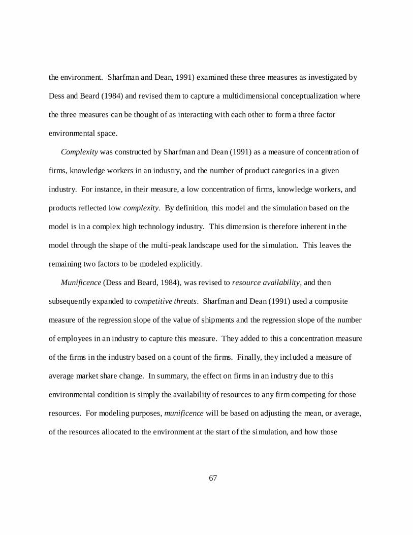
67
the environment. Sharfman and Dean, 1991) examined these three measures as investigated by
Dess and Beard (1984) and revised them to capture a multidimensional conceptualization where
the three measures can be thought of as interacting with each other to form a three factor
environmental space.
Complexity was constructed by Sharfman and Dean (1991) as a measure of concentration of
firms, knowledge workers in an industry, and the number of product categories in a given
industry. For instance, in their measure, a low concentration of firms, knowledge workers, and
products reflected low complexity. By definition, this model and the simulation based on the
model is in a complex high technology industry. This dimension is therefore inherent in the
model through the shape of the multi-peak landscape used for the simulation. This leaves the
remaining two factors to be modeled explicitly.
Munificence (Dess and Beard, 1984), was revised to resource availability, and then
subsequently expanded to competitive threats. Sharfman and Dean (1991) used a composite
measure of the regression slope of the value of shipments and the regression slope of the number
of employees in an industry to capture this measure. They added to this a concentration measure
of the firms in the industry based on a count of the firms. Finally, they included a measure of
average market share change. In summary, the effect on firms in an industry due to this
environmental condition is simply the availability of resources to any firm competing for those
resources. For modeling purposes, munificence will be based on adjusting the mean, or average,
of the resources allocated to the environment at the start of the simulation, and how those

68
resources are replenished throughout the simulation. See Figure 8 for examples of how this will
be implement in the model.
Figure 8 - Resource Munificence: Using Different Means
Dynamism, in the revised measure, includes both market and technological instability.
Dynamism has been operationalized in empirical studies to include the number of shipments of
goods made by a company over a period of time, the number of employees in an industry over a
period of time, and the average number of patents in an industry over time. For instance, in high
technology industries this equates to the number of patents applied for. Therefore, the higher the
count of patent applications in an industry, the more unstable the environment in that industry is.
Following the guidelines for straightforward model development, I use the concept of resource
distribution variance for dynamism. Note that munificence is conceptualized as the mean of a
resource distribution curve. It follows that dynamism is the shape, or distribution of the
resources around the mean. See Figure 9 for an example of how this will be varied in the model.
Mean = -2 0 +2
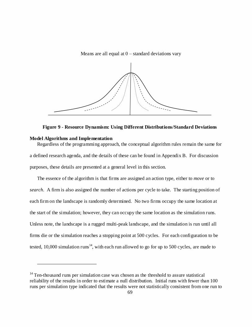
69
Figure 9 - Resource Dynamism: Using Different Distributions/Standard Deviations
Model Algorithms and Implementation
Regardless of the programming approach, the conceptual algorithm rules remain the same for
a defined research agenda, and the details of these can be found in Appendix B. For discussion
purposes, these details are presented at a general level in this section.
The essence of the algorithm is that firms are assigned an action type, either to move or to
search. A firm is also assigned the number of actions per cycle to take. The starting position of
each firm on the landscape is randomly determined. No two firms occupy the same location at
the start of the simulation; however, they can occupy the same location as the simulation runs.
Unless note, the landscape is a rugged multi-peak landscape, and the simulation is run until all
firms die or the simulation reaches a stopping point at 500 cycles. For each configuration to be
tested, 10,000 simulation runs14, with each run allowed to go for up to 500 cycles, are made to
14 Ten-thousand runs per simulation case was chosen as the threshold to assure statistical
reliability of the results in order to estimate a null distribution. Initial runs with fewer than 100
runs per simulation type indicated that the results were not statistically consistent from one run to
Means are all equal at 0 – standard deviations vary
70
insure that the random factors employed in the simulation algorithms are sampled sufficiently to
achieve repeatable results. Data are collected on each step of the simulation, all 500 steps, for all
10,000 runs. To collect enough data to test one hypothesis required 250,000 simulation runs of
up to 500 steps per run. I collected approximately eight gigabytes of data to test the hypotheses.
What follows is a more detailed discussion of the implementation. To achieve Red Queen
competition the number of firm actions, the relative rate of the actions, the type of actions, and
the strategy to execute the actions need to be controlled, and varied. The number of total cycles
in the simulation controls the number of actions. Also, the landscape that the firms compete on
needs to be controlled for the shape of the landscape (resources available on each unique location
on the landscape), the mean of these resources, and the distribution of these resources on the
landscape. A stochastic process was chosen to do this. The most appropriate programming
environment is agent-based as noted earlier. Agent-based means the focus of the simulation
controls is on the agents, which in my case are the firms. The agents can be programmed with
specific behaviors, just a like a firm behaves, so I can mimic how a firm in Red Queen
competition behaves.
Once the decision to use an agent-based program was made, the next choice is the specific
programming language and development environment to use. There are several choices for the
programming language and environment. After reading the available literature on published
another due to the random nature of some of the decisions firms can make on the landscape.
Increasing the runs to 1,000 resolved the issues. A safety factor of 10 was used to insure that the
results consistently represented the null distribution. Ten-thousand is not an uncommon number
to use for the number of runs in a simulation of this nature.
71
research using agent-based programs, I narrowed the selection to two candidates: RePast for
Java, or RePastJ, and NetLogo. After working with both programs, and considerable
consultation with programmers and researchers in the field, I selected NetLogo, version 4.1
(Wylinski, 1989), to implement the model.
My original goal was to have a trained programmer implement my specification. I therefore
engaged several programmers to review my specification for the six months that it took to
develop it. After testing the programming environments myself, I realized that my programming
background and prior experience was sufficient to implement my own code. Therefore, I
developed the entire program contained in Appendix B. Netlogo provides a nearly barren user
interface – you can gain some insight into the model I developed by reviewing the controls
displayed in Appendix A, a screen shot of the user interface panel from my model. To insure
that I followed best practices, and to gain outside objective reviews, I sent my code to more
experienced programmers to vet it, and I also made good use of the NetLogo programmer‘s
forum during the implementation and testing phase. I would suggest that in general, it is still
better for most researchers to hire someone or partner with someone to write the simulation code
for them. That being said, I do feel I gained even more insight into the simulation process, and
how the Red Queen competition works by developing my own simulation program. And, this
was a significant aid when it came time to interpret the results. Specifically, it helped me
identify how artifacts in the simulation, rather than the logic of competition, affected the results.
72
NetLogo incorporates the use of a User Interface Panel. (See Appendix A for a screen-shot
of the user interface panel.) Once the program is loaded and started, the user specifies the
following information:
1. The type of landscape the firms will compete on (simple peak, rugged multi-peak, or
random). This was typically set at rugged multi-peak.
2. The number of firms in the environment (from one to 100). This was typically set at
two.
3. The ratio of Red Queen Firms (termed New Firms in the simulation panel) to Rival
Firms. This was typically set at 50/50.
4. The strategy for each firm – this was set for the Red Queen firm, and the Rival firm
(Random Direction, Random Opportunistic, or Pure Opportunistic. Note that other
strategies were developed for post-hoc analysis).
5. The number of moves to be made by each firm for each cycle of the simulation (from
0 up).
6. The number of spaces to be leaped over is called the search-distance, for each firm
(from 0 up to 20).
7. The starting wealth of each firm (from 0 up, typically set at 20).
8. If action cost was dynamic or fixed by the user. Dynamic cost allocation charged the
average available resources on the landscape for a move, and 33% of the average for
a look per space during a search. If the average resource per square on the landscape
was 3 units, then the cost to move was also 3 units, and the cost to look was one unit.
73
If the cost allocation was fixed by the user, the user selected a discrete amount for
both action types. The same cost allocation was used for all firm types.
9. The mean or average resources to be allocated on the landscape. (typically set at 10).
10. The variance of the resources to be allocated on the landscape. (varied from 0 to 10,
and was determined as the standard deviation of the resources).
11. The replenishment rate of resources, set as the number of units to be replenished per
cycle. (typically set at 10, which replenished a location as soon as the next cycle of
the simulation started.)
12. Note – other factors were developed in the simulation model for post-hoc exploration
and will be reported in Chapter Four where appropriate.
Step 5 – Verification of the computational representation. All software programs required
testing to insure that they deliver what is expected of them15. NetLogo‘s user interface panel
allowed me to program in a visual link to the landscape where the firms executed their actions
and strategy. This is a near real-time visualization in that each move of the firm is visible to the
user. The layout of the landscape is visible. The landscape was programmed so that each square
was colored green – the more resources on a square, the darker the green, in essence signaling
the amount of money, or in an ecosystem sense, the amount of vegetation, on the square. When
the resources are depleted, the square turns black until it is replenished.
15 I spent five years as the director research and development of software at a software
development firm that was associated with AT&T Bell Labs. As a result I was exposed to the
science, and the art, of software performance verification. I incorporated this experience in the
verification of the simulation program. My approach parallels the one called for by Rand and
Rust (2010).
74
I also designed in counters and line graphs to monitor the viability of the firms and their
wealth accumulation. The speed of the simulation is controlled from the user panel so the user
can run the events in what would be described as slow-motion, where the movement of a firm
from one location to another location takes several sections. This allowed me to visualize the
competition, watch resource accumulation, and verify that the strategy programmed into a firm
was being acted out.
Test modes were also invoked. For instance, one test mode used a flat landscape with the
resource value set to the same amount on every location. In this mode, running one firm at a
time for 10,000 runs, the results should be the same. Other verifications included swapping the
roles between the Red Queen Firm and the Rival Firm and running the simulation to confirm that
the behaviors resulted were as expected. The program was adjusted in each case until all of the
testing requirements were satisfied.
Step 6 - Run the simulation to collect data. NetLogo 4.1 supports the use of a batch program
to runs a series of simulations with varying parameters set by the user. This program is called
Behavior Space. I used this to run 10,000 runs per batch. The data collected were formatted as a
.csv file which was imported into Microsoft Excel, the 2007 edition. A 10,000 simulation run,
with 500 cycles per simulation, is the approximate limit of Excel (some 167,000 columns). I
wrote a series of macros to consolidate the data into summary tables, and then a second
consolidation to prepare the data for statistical analysis and graphing.
To collect data to test the hypotheses, various attributes of the simulation were changed.
These configurations are detailed in Table 5 shown below.
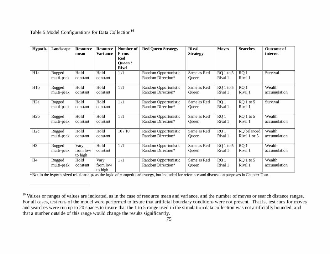
75
Table 5 Model Configurations for Data Collection16
Hypoth. Landscape Resource
mean
Resource
Variance
Number of
Firms
Red
Queen /
Rival
Red Queen Strategy Rival
Strategy
Moves Searches Outcome of
interest
H1a Rugged
multi-peak
Hold
constant
Hold
constant
1 /1 Random Opportunistic
Random Direction*
Same as Red
Queen
RQ 1 to 5
Rival 1
RQ 1
Rival 1
Survival
H1b Rugged multi-peak
Hold constant
Hold constant
1 /1 Random Opportunistic Random Direction*
Same as Red Queen
RQ 1 to 5 Rival 1
RQ 1 Rival 1
Wealth accumulation
H2a Rugged multi-peak
Hold constant
Hold constant
1 /1 Random Opportunistic Random Direction*
Same as Red Queen
RQ 1 Rival 1
RQ 1 to 5 Rival 1
Survival
H2b Rugged
multi-peak
Hold
constant
Hold
constant
1 /1 Random Opportunistic
Random Direction*
Same as Red
Queen
RQ 1
Rival 1
RQ 1 to 5
Rival 1
Wealth
accumulation
H2c Rugged multi-peak
Hold constant
Hold constant
10 / 10 Random Opportunistic Random Direction*
Same as Red Queen
RQ 1 Rival 1
RQ balanced Rival 1 or 5
Wealth accumulation
H3 Rugged multi-peak
Vary from low to high
Hold constant
1 /1 Random Opportunistic Random Direction*
Same as Red Queen
RQ 1 to 5 Rival 1
RQ 1 Rival 1
Wealth accumulation
H4 Rugged
multi-peak
Hold
constant
Vary
from low to high
1 /1 Random Opportunistic
Random Direction*
Same as Red
Queen
RQ 1
Rival 1
RQ 1 to 5
Rival 1
Wealth
accumulation
*Not in the hypothesized relationships as the logic of competition/strategy, but included for reference and discussion purposes in Chapter Four.
16 Values or ranges of values are indicated, as in the case of resource mean and variance, and the number of moves or search distance ranges.
For all cases, test runs of the model were performed to insure that artificial boundary conditions were not present. That is , test runs for moves
and searches were run up to 20 spaces to insure that the 1 to 5 range used in the simulation data collection was not artificially bounded, and
that a number outside of this range would change the results significantly.

76
Analysis Methodology
Simulations were run and data collected per Table 5 above. The output results are charted as
firm survival or firm performance curves using data from the simulations. Typically, each chart consists
of five discrete but related competitive scenarios that were simulated. For example, in the case of H1a
escalated move-based activity is tested using five levels of escalation. Each level of escalation
represents a series of 10,000 simulation runs. In turn, the mean of the results of each of the five series is
plotted on a chart to represent the series. This mean is generated from the data from 10,000 runs, with
up to 500 cycles per run, to create the results for the plots, and to produce the results for statistical
analysis.
A strong point of simulation based research is its construct validity, which is accurate specification
and measurement of constructs (Cook & Campbell, 1979). As noted by Rosenthal and Rosenow (1991),
simulation requires precise specification of the essential components modeled and their measures and
therefore avoids the signal-to-noise measurement problems that affects construct validity in empirical
research. Data produced by simulations are therefore free of measurement errors associated with
empirical data and consequently convergent and discriminant validity are not an issue (Campbell &
Fiske, 1959). Therefore, following current practices in evaluating hypothesized predictions with
simulation data, the means of the key measures for Red Queen and Rival firms, firm performance and
firm survival, are compared, per March (1991), Ganco (2009), Rand and Rust (2010), and Rivkin (2000)
and depicted in the wealth accumulation performance charts and survival charts17. Confidence intervals
17 Additional analysis using methods such as regression or latent-growth curve, which are typically
used for empirical data analysis, are not required for the simulation data produced. As noted in a
forthcoming article, Rust, W., and Rust, R. (2010) Agent-based modeling in Marketing: Guidelines for
77
were calculated at 99% for the means reported for each firm type to test if the results between the Red
Queen firm and the Rival firm were significantly different (Cohen, Cohen, West, & Aiken, 2003; Witte
& Witte, 2004). These results are reported for each hypothesis in a separate table with other descriptive
statistics, and plotted in an accompanying figure. As noted in the footnote for Table 5, and repeated
here for emphasis, values or ranges of values are indicated, as in the case of resource mean and variance,
and the number of moves or search-distance ranges. For all cases, test runs of the model were
performed to insure that artificial boundary conditions were not present. For example, simulation runs
for move and search-distance activities were completed by varying the move or search-distance values
from one to 20 spaces to insure that the one to five spaces used in the simulation data collection were not
artificial boundaries. The results confirmed that the range of one to five was appropriate to test the
hypotheses. Similar verifications were made regarding non-hypothesized and hypothesize variables,
including the size of the landscape, initial resources given to firms, and the number of firms competing
at one time on the landscape.
Measures and Variable Definitions
The following were used in the simulation.
Dependent Variables
For H1a and H2a the dependent variable is firm survival. Firm survival is measured in terms of
the number of cycles that a firm competes in while its accumulated wealth is greater than zero. For each
cycle the firm survives, this value is incremented by one. A zero value of wealth, or a negative value, is
rigor, means comparison with confidence interval evaluation is the standard method of hypothesis
testing.
78
analogous to bankruptcy and signals the death of the firm. The simulation continues to run until no
firms survive, or the limit of 500 cycles is reached.
For H1b, H2b, H3, and H4 the dependent variable is performance, measured as wealth
accumulation. With each cycle of the simulation a firm has the opportunity to undertake an action. The
results of the action affect the firm‘s accumulated wealth. Each action has results in a cost to the firm
and an earning of resources. The net of the cost to the firm less the resources earned by the firm is added
or subtracted to the firm‘s current wealth.
Main Explanatory Variables
Two types of actions are specified: move based and search-distance based. H1, H2, and H4
make predictions using the move based activity. H3 makes a prediction using search-distance activity.
When a firm moves on the landscape, it changes its location one space on the grid at a time, and it
travels on contiguous spaces. When a firm moves, it does so in increments of one space at a time, from
one to five spaces. On the other hand, a firm that uses search-distance may skip, or jump over a
location. A firm that is uses a search-distance of three will jump to a location, in a straight path, that is
three spaces away from its current location. That is, there will be two spaces between the current
location and the future location that the firm does not land on. These two actions are illustrated in
Figure 10 below. The move based activity is shown for a firm that is initially on location 43, and moves
to location 37, location 31, and finally to location 25. The search-distance activity is shown for a firm
that is initially on location 49 and with one jump arrives on location 25. Note that two locations, 41 and
33, were skipped over by this firm.
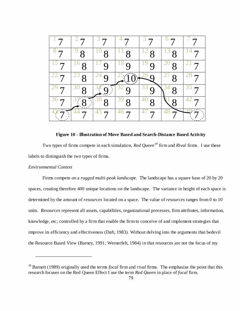
79
1 7
2
7 3
7 4
7 5
7 6
7 7
7 8
7 9
8 10
8 11
8 12
8 13
8 14
7 15
7 16
8 17
9 18
9 19
9 20
8 21
7 22
7 23
8 24
9 25
10 26
9 27
8 28
7 29
7 30
8 31
9 32
9 33
9 34
8 35
7 36
7 37
8 38
8 39
8 40
8 41
8 42
7 43
7 44
7 45
7 46
7 47
7 48
7 49
7
Figure 10 - Illustration of Move Based and Search-Distance Based Activity
Two types of firms compete in each simulation, Red Queen18 firm and Rival firms. I use these
labels to distinguish the two types of firms.
Environmental Context
Firms compete on a rugged multi-peak landscape. The landscape has a square base of 20 by 20
spaces, creating therefore 400 unique locations on the landscape. The variance in height of each space is
determined by the amount of resources located on a space. The value of resources ranges from 0 to 10
units. Resources represent all assets, capabilities, organizational processes, firm attributes, information,
knowledge, etc; controlled by a firm that enable the firm to conceive of and implement strategies that
improve its efficiency and effectiveness (Daft, 1983). Without delving into the arguments that bedevil
the Resource Based View (Barney, 1991; Wernerfelt, 1984) in that resources are not the focus of my
18 Barnett (1989) originally used the terms focal firm and rival firms. The emphasize the point that this
research focuses on the Red Queen Effect I use the term Red Queen in place of focal firm.
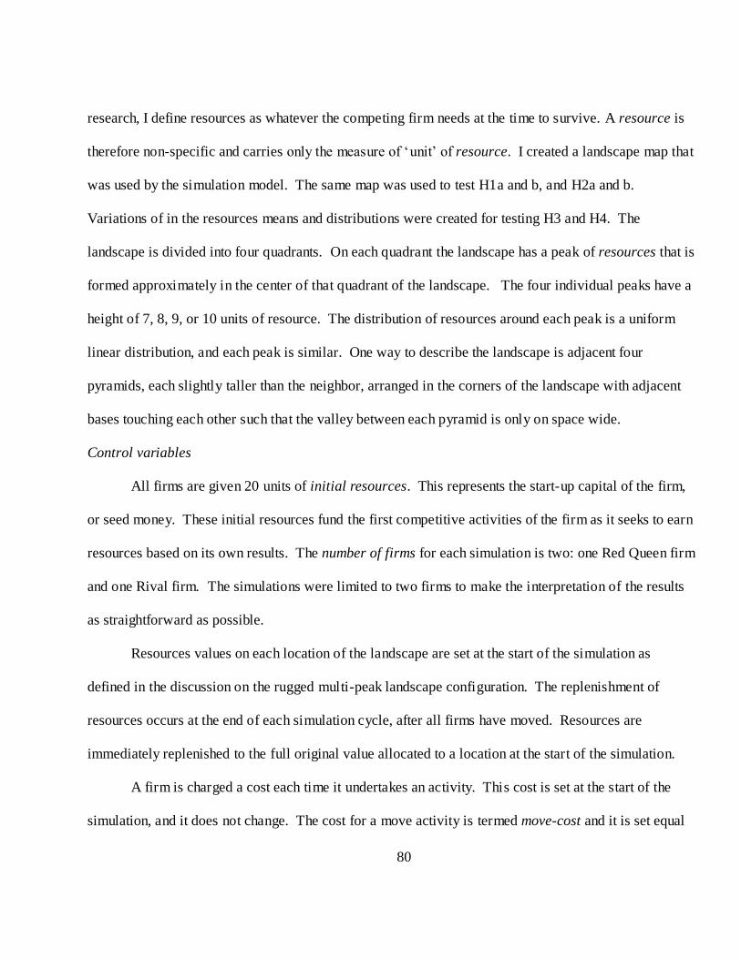
80
research, I define resources as whatever the competing firm needs at the time to survive. A resource is
therefore non-specific and carries only the measure of ‗unit‘ of resource. I created a landscape map that
was used by the simulation model. The same map was used to test H1a and b, and H2a and b.
Variations of in the resources means and distributions were created for testing H3 and H4. The
landscape is divided into four quadrants. On each quadrant the landscape has a peak of resources that is
formed approximately in the center of that quadrant of the landscape. The four individual peaks have a
height of 7, 8, 9, or 10 units of resource. The distribution of resources around each peak is a uniform
linear distribution, and each peak is similar. One way to describe the landscape is adjacent four
pyramids, each slightly taller than the neighbor, arranged in the corners of the landscape with adjacent
bases touching each other such that the valley between each pyramid is only on space wide.
Control variables
All firms are given 20 units of initial resources. This represents the start-up capital of the firm,
or seed money. These initial resources fund the first competitive activities of the firm as it seeks to earn
resources based on its own results. The number of firms for each simulation is two: one Red Queen firm
and one Rival firm. The simulations were limited to two firms to make the interpretation of the results
as straightforward as possible.
Resources values on each location of the landscape are set at the start of the simulation as
defined in the discussion on the rugged multi-peak landscape configuration. The replenishment of
resources occurs at the end of each simulation cycle, after all firms have moved. Resources are
immediately replenished to the full original value allocated to a location at the start of the simulation.
A firm is charged a cost each time it undertakes an activity. This cost is set at the start of the
simulation, and it does not change. The cost for a move activity is termed move-cost and it is set equal

81
to the average resource units on the overall landscape for each number of moves made by a firm on a
single cycle of the simulation. The cost of a search-distance activity is termed search-distance-cost and
it is set equal to the combination of the amount of one move-cost and a variable amount of look-cost.
Regardless of the search-distance, the move-cost component is always equal to one move-cost. The
factor to account for the spaces examined during the search-distance activity is determined by
multiplying the look-cost times the search-distance value. The look-cost can be thought of as research
cost or resources expended in the examination of looking at the location prior to moving to the location,
or even skipping over the location.
Only one firm strategy, Random Opportunistic, is used for the testing of all hypotheses. An
alternative strategy, Random Direction, is employed during the post-hoc analysis. Both firm types
always use the same strategy for the entire simulation.
Results
For convenience, each hypothesis is presented prior to the discussion of the results for the
hypothesis. The testing details and a discussion of the results for each hypothesis are reported after the
hypothesis is presented. Variable means, standard deviations, and the results for each hypothesis test are
then reported. And finally, the plotted means of the key variables used in testing each hypothesis are
presented as a visual representation of the results.
The results from the hypotheses testing are mixed. In general, partial to full support is found for
hypotheses that test a move action. However, the hypotheses that test a search action are in general not
fully supported.
Hypothesis 1a: A new firm engaged in a higher rate of competitive moves for resources in their
environment, relative to a rival firm’s rate of moves, will initially have a greater survival rate than
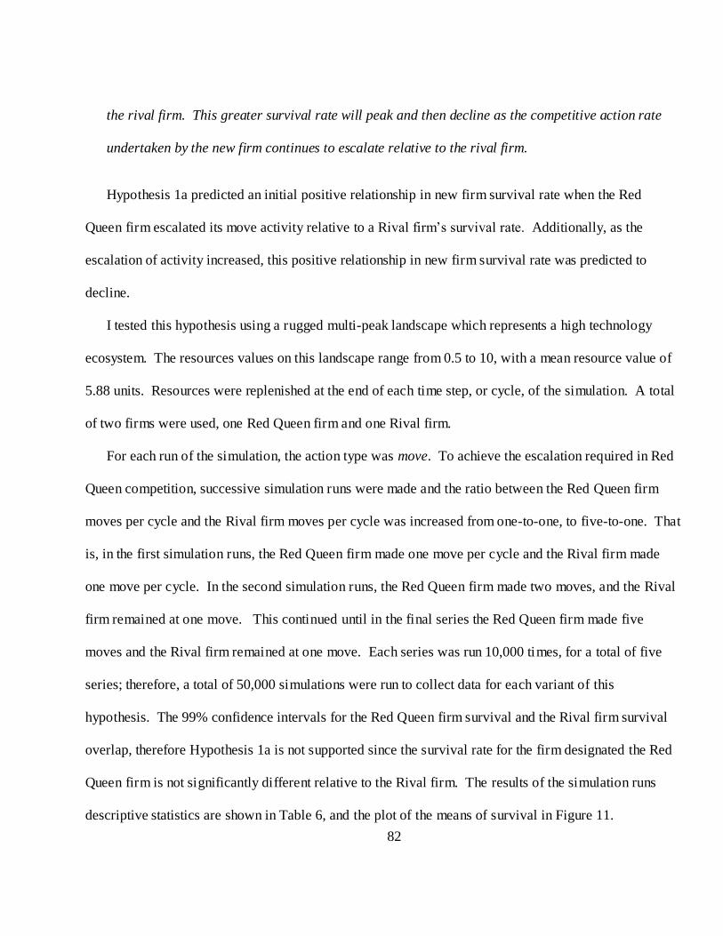
82
the rival firm. This greater survival rate will peak and then decline as the competitive action rate
undertaken by the new firm continues to escalate relative to the rival firm.
Hypothesis 1a predicted an initial positive relationship in new firm survival rate when the Red
Queen firm escalated its move activity relative to a Rival firm‘s survival rate. Additionally, as the
escalation of activity increased, this positive relationship in new firm survival rate was predicted to
decline.
I tested this hypothesis using a rugged multi-peak landscape which represents a high technology
ecosystem. The resources values on this landscape range from 0.5 to 10, with a mean resource value of
5.88 units. Resources were replenished at the end of each time step, or cycle, of the simulation. A total
of two firms were used, one Red Queen firm and one Rival firm.
For each run of the simulation, the action type was move. To achieve the escalation required in Red
Queen competition, successive simulation runs were made and the ratio between the Red Queen firm
moves per cycle and the Rival firm moves per cycle was increased from one-to-one, to five-to-one. That
is, in the first simulation runs, the Red Queen firm made one move per cycle and the Rival firm made
one move per cycle. In the second simulation runs, the Red Queen firm made two moves, and the Rival
firm remained at one move. This continued until in the final series the Red Queen firm made five
moves and the Rival firm remained at one move. Each series was run 10,000 times, for a total of five
series; therefore, a total of 50,000 simulations were run to collect data for each variant of this
hypothesis. The 99% confidence intervals for the Red Queen firm survival and the Rival firm survival
overlap, therefore Hypothesis 1a is not supported since the survival rate for the firm designated the Red
Queen firm is not significantly different relative to the Rival firm. The results of the simulation runs
descriptive statistics are shown in Table 6, and the plot of the means of survival in Figure 11.

83
Table 6 H1a Descriptive Statistics and Confidence Intervals – Survival of Firms
Hypothesis
and Ratio
of Red
Queen to
Rival
Moves
Mean
Red
Queen
Survival
Mean
Rival
Survival
SD
Red
Queen
Survival
SD
Rival
Survival
Lower
Conf.
Interval
of Red
Queen
Survival
Upper
Conf.
Interval
of Red
Queen
Survival
Lower
Conf.
Interval
of Rival
Survival
Upper
Conf.
Interval
of Rival
Survival
H1a – 1 500.0 500.0 0.0 0.0 500.0 500.0 500.0 500.0
H1a - 2 500.0 500.0 0.0 0.0 500.0 500.0 500.0 500.0
H1a - 3 500.0 500.0 0.0 0.0 500.0 500.0 500.0 500.0
H1a - 4 500.0 500.0 0.0 0.0 500.0 500.0 500.0 500.0
H1a - 5 500.0 500.0 0.0 0.0 500.0 500.0 500.0 500.0
n=10,000
Confidence intervals calculated at 99%
*indicates means are different at .01 significance level
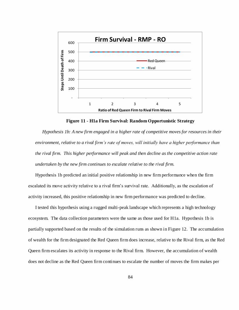
84
Figure 11 - H1a Firm Survival: Random Opportunistic Strategy
Hypothesis 1b: A new firm engaged in a higher rate of competitive moves for resources in their
environment, relative to a rival firm’s rate of moves, will initially have a higher performance than
the rival firm. This higher performance will peak and then decline as the competitive action rate
undertaken by the new firm continues to escalate relative to the rival firm.
Hypothesis 1b predicted an initial positive relationship in new firm performance when the firm
escalated its move activity relative to a rival firm‘s survival rate. Additionally, as the escalation of
activity increased, this positive relationship in new firm performance was predicted to decline.
I tested this hypothesis using a rugged multi-peak landscape which represents a high technology
ecosystem. The data collection parameters were the same as those used for H1a. Hypothesis 1b is
partially supported based on the results of the simulation runs as shown in Figure 12. The accumulation
of wealth for the firm designated the Red Queen firm does increase, relative to the Rival firm, as the Red
Queen firm escalates its activity in response to the Rival firm. However, the accumulation of wealth
does not decline as the Red Queen firm continues to escalate the number of moves the firm makes per
-
100
200
300
400
500
600
1 2 3 4 5
Ste
ps
Un
til D
eat
h o
f Fir
m
Ratio of Red Queen Firm to Rival Firm Moves
Firm Survival - RMP - RO
Red Queen
Rival
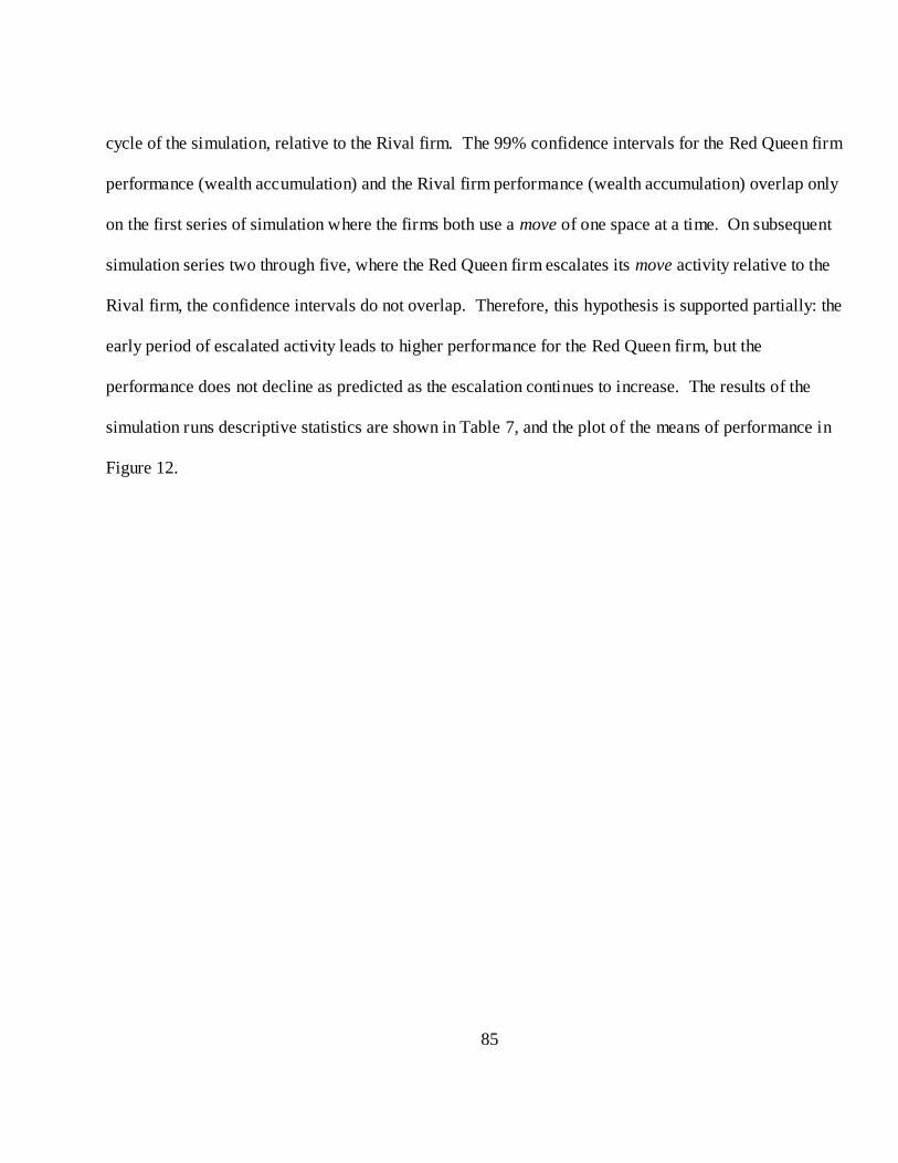
85
cycle of the simulation, relative to the Rival firm. The 99% confidence intervals for the Red Queen firm
performance (wealth accumulation) and the Rival firm performance (wealth accumulation) overlap only
on the first series of simulation where the firms both use a move of one space at a time. On subsequent
simulation series two through five, where the Red Queen firm escalates its move activity relative to the
Rival firm, the confidence intervals do not overlap. Therefore, this hypothesis is supported partially: the
early period of escalated activity leads to higher performance for the Red Queen firm, but the
performance does not decline as predicted as the escalation continues to increase. The results of the
simulation runs descriptive statistics are shown in Table 7, and the plot of the means of performance in
Figure 12.
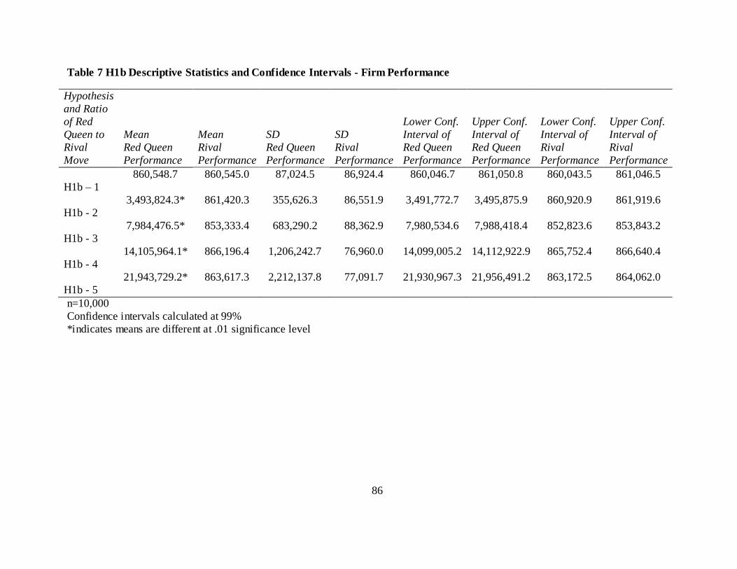
86
Table 7 H1b Descriptive Statistics and Confidence Intervals - Firm Performance
Hypothesis
and Ratio
of Red
Queen to
Rival
Move
Mean
Red Queen
Performance
Mean
Rival
Performance
SD
Red Queen
Performance
SD
Rival
Performance
Lower Conf.
Interval of
Red Queen
Performance
Upper Conf.
Interval of
Red Queen
Performance
Lower Conf.
Interval of
Rival
Performance
Upper Conf.
Interval of
Rival
Performance
H1b – 1
860,548.7 860,545.0 87,024.5 86,924.4 860,046.7 861,050.8 860,043.5 861,046.5
H1b - 2
3,493,824.3* 861,420.3 355,626.3 86,551.9 3,491,772.7 3,495,875.9 860,920.9 861,919.6
H1b - 3
7,984,476.5* 853,333.4 683,290.2 88,362.9 7,980,534.6 7,988,418.4 852,823.6 853,843.2
H1b - 4
14,105,964.1* 866,196.4 1,206,242.7 76,960.0 14,099,005.2 14,112,922.9 865,752.4 866,640.4
H1b - 5
21,943,729.2* 863,617.3 2,212,137.8 77,091.7 21,930,967.3 21,956,491.2 863,172.5 864,062.0
n=10,000
Confidence intervals calculated at 99%
*indicates means are different at .01 significance level

87
Figure 12 – H1b Wealth Accumulation: Random Opportunistic Strategy
Hypothesis 2a: New firms that engage in more distant search actions will exhibit higher failure
rates over time than rival firms that engage in more local search actions.
Hypothesis 2a predicted an initial positive relationship in new firm survival rate when the firm
escalated its search-distance activity relative to a rival firm‘s survival rate. Additionally, as the
escalation of activity increased, this positive relationship in new firm survival rate was predicted to
decline.
Similar to Hypothesis 1a and 1b, I tested this hypothesis using a rugged multi-peak landscape which
represents a high technology ecosystem. The resources values on this landscape range from 0.5 to 10,
with a mean resource value of 5.88 units. Resources were replenished at the end of each time step, or
cycle, of the simulation. A total of two firms were used, one Red Queen firm and one Rival firm.
For each run of the simulation, the action type was search-distance. To achieve the escalation
required in Red Queen competition, successive simulation runs were made and the ratio between the
Red Queen firm search-distance per cycle and the Rival firm search-distance per cycle was increased
from one-to-one, to five-to-one. That is, in the first simulation runs, since the search-distance was one
-
5,000,000
10,000,000
15,000,000
20,000,000
25,000,000
1 2 3 4 5
Firm
Pe
rfo
rman
ce
Ratio of Red Queen Firm to Rival Firm Moves
Wealth Accumulation - Rugged Multi-Peak
Red Queen
Rival
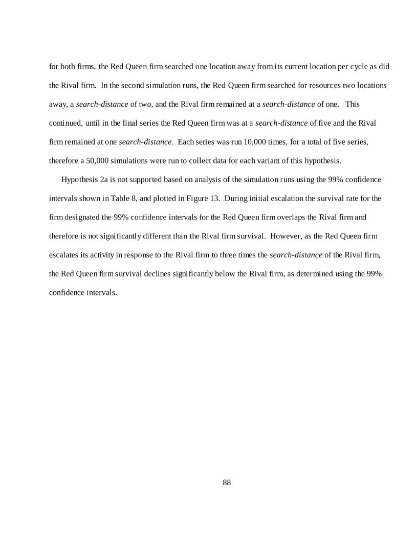
88
for both firms, the Red Queen firm searched one location away from its current location per cycle as did
the Rival firm. In the second simulation runs, the Red Queen firm searched for resources two locations
away, a search-distance of two, and the Rival firm remained at a search-distance of one. This
continued, until in the final series the Red Queen firm was at a search-distance of five and the Rival
firm remained at one search-distance. Each series was run 10,000 times, for a total of five series,
therefore a 50,000 simulations were run to collect data for each variant of this hypothesis.
Hypothesis 2a is not supported based on analysis of the simulation runs using the 99% confidence
intervals shown in Table 8, and plotted in Figure 13. During initial escalation the survival rate for the
firm designated the 99% confidence intervals for the Red Queen firm overlaps the Rival firm and
therefore is not significantly different than the Rival firm survival. However, as the Red Queen firm
escalates its activity in response to the Rival firm to three times the search-distance of the Rival firm,
the Red Queen firm survival declines significantly below the Rival firm, as determined using the 99%
confidence intervals.
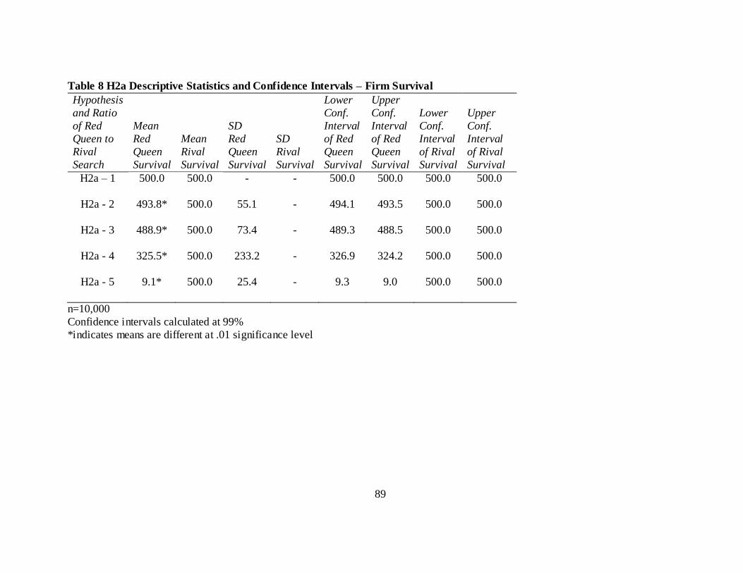
89
Table 8 H2a Descriptive Statistics and Confidence Intervals – Firm Survival
Hypothesis
and Ratio
of Red
Queen to
Rival
Search
Mean
Red
Queen
Survival
Mean
Rival
Survival
SD
Red
Queen
Survival
SD
Rival
Survival
Lower
Conf.
Interval
of Red
Queen
Survival
Upper
Conf.
Interval
of Red
Queen
Survival
Lower
Conf.
Interval
of Rival
Survival
Upper
Conf.
Interval
of Rival
Survival
H2a – 1 500.0 500.0 - - 500.0 500.0 500.0 500.0
H2a - 2 493.8* 500.0 55.1 - 494.1 493.5 500.0 500.0
H2a - 3 488.9* 500.0 73.4 - 489.3 488.5 500.0 500.0
H2a - 4 325.5* 500.0 233.2 - 326.9 324.2 500.0 500.0
H2a - 5 9.1* 500.0 25.4 - 9.3 9.0 500.0 500.0
n=10,000
Confidence intervals calculated at 99%
*indicates means are different at .01 significance level
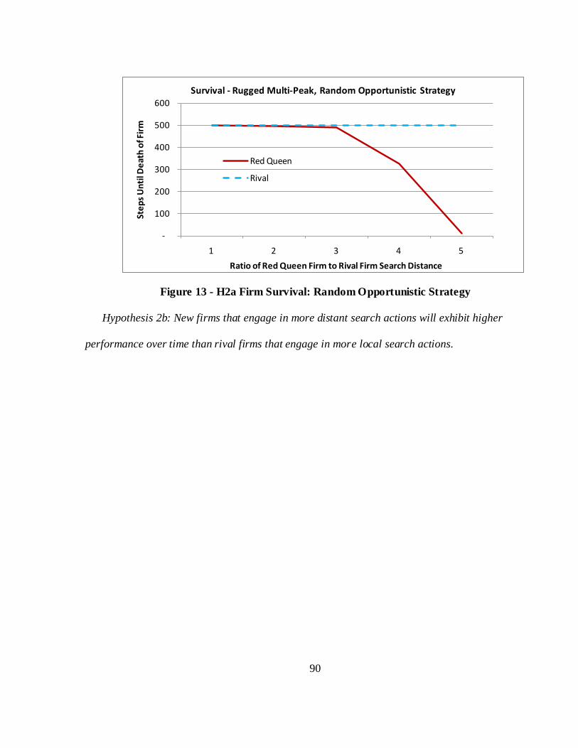
90
Figure 13 - H2a Firm Survival: Random Opportunistic Strategy
Hypothesis 2b: New firms that engage in more distant search actions will exhibit higher
performance over time than rival firms that engage in more local search actions.
-
100
200
300
400
500
600
1 2 3 4 5
Ste
ps
Un
til D
eat
h o
f Fir
m
Ratio of Red Queen Firm to Rival Firm Search Distance
Survival - Rugged Multi-Peak, Random Opportunistic Strategy
Red Queen
Rival
91
Table 9 H2b Descriptive Statistics and Confidence Intervals – Firm Performance
Hypothesis
and Ratio of
Red Queen to
Rival Search
Mean
Red Queen
Performance
Mean
Rival
Performance
SD
Red Queen
Performance
SD
Rival
Performance
Lower Conf.
Interval of
Red Queen
Performance
Upper Conf.
Interval of
Red Queen
Performance
Lower Conf.
Interval of
Rival
Performance
Upper Conf.
Interval of
Rival
Performance
H2b – 1 859,546.2 864,238.2 73,688.4 88,594.4 859,121.0 859,971.3 863,727.1 864,749.3
H2b – 2 591,827.8* 873,075.3 96,336.1 78,473.8 591,272.1 592,383.6 872,622.5 873,528.0
H2b – 3 341,795.7* 862,216.8 87,090.3 75,872.3 341,293.3 342,298.2 861,779.1 862,654.5
H2b – 4 61,875.8* 876,549.7 68,313.8 76,271.7 61,481.7 62,269.9 876,109.7 876,989.8
H2b – 5 180.5* 867,242.5 2,342.3 89,748.6 167.0 194.0 866,724.7 867,760.2
n=10,000
Confidence intervals calculated at 99%
*indicates means are different at .01 significance level
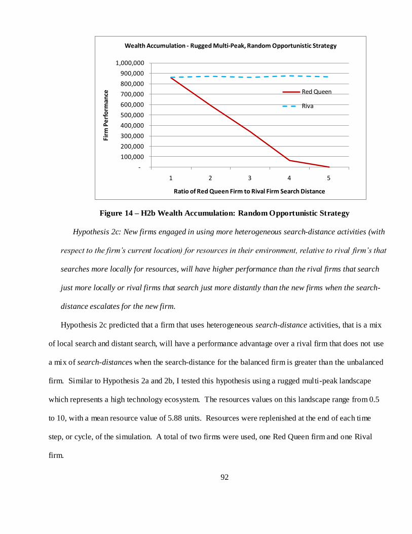
92
Figure 14 – H2b Wealth Accumulation: Random Opportunistic Strategy
Hypothesis 2c: New firms engaged in using more heterogeneous search-distance activities (with
respect to the firm’s current location) for resources in their environment, relative to rival firm’s that
searches more locally for resources, will have higher performance than the rival firms that search
just more locally or rival firms that search just more distantly than the new firms when the search-
distance escalates for the new firm.
Hypothesis 2c predicted that a firm that uses heterogeneous search-distance activities, that is a mix
of local search and distant search, will have a performance advantage over a rival firm that does not use
a mix of search-distances when the search-distance for the balanced firm is greater than the unbalanced
firm. Similar to Hypothesis 2a and 2b, I tested this hypothesis using a rugged multi-peak landscape
which represents a high technology ecosystem. The resources values on this landscape range from 0.5
to 10, with a mean resource value of 5.88 units. Resources were replenished at the end of each time
step, or cycle, of the simulation. A total of two firms were used, one Red Queen firm and one Rival
firm.
-
100,000
200,000
300,000
400,000
500,000
600,000
700,000
800,000
900,000
1,000,000
1 2 3 4 5
Firm
Pe
rfo
rman
ce
Ratio of Red Queen Firm to Rival Firm Search Distance
Wealth Accumulation - Rugged Multi-Peak, Random Opportunistic Strategy
Red Queen
Riva
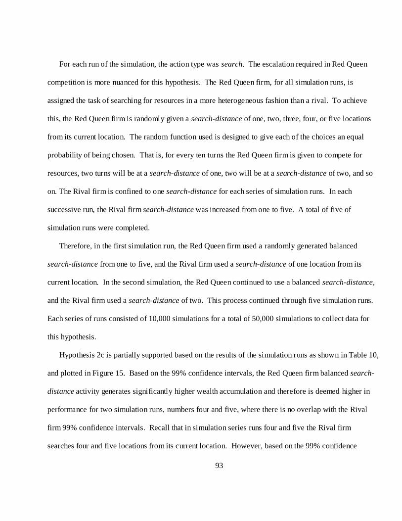
93
For each run of the simulation, the action type was search. The escalation required in Red Queen
competition is more nuanced for this hypothesis. The Red Queen firm, for all simulation runs, is
assigned the task of searching for resources in a more heterogeneous fashion than a rival. To achieve
this, the Red Queen firm is randomly given a search-distance of one, two, three, four, or five locations
from its current location. The random function used is designed to give each of the choices an equal
probability of being chosen. That is, for every ten turns the Red Queen firm is given to compete for
resources, two turns will be at a search-distance of one, two will be at a search-distance of two, and so
on. The Rival firm is confined to one search-distance for each series of simulation runs. In each
successive run, the Rival firm search-distance was increased from one to five. A total of five of
simulation runs were completed.
Therefore, in the first simulation run, the Red Queen firm used a randomly generated balanced
search-distance from one to five, and the Rival firm used a search-distance of one location from its
current location. In the second simulation, the Red Queen continued to use a balanced search-distance,
and the Rival firm used a search-distance of two. This process continued through five simulation runs.
Each series of runs consisted of 10,000 simulations for a total of 50,000 simulations to collect data for
this hypothesis.
Hypothesis 2c is partially supported based on the results of the simulation runs as shown in Table 10,
and plotted in Figure 15. Based on the 99% confidence intervals, the Red Queen firm balanced search-
distance activity generates significantly higher wealth accumulation and therefore is deemed higher in
performance for two simulation runs, numbers four and five, where there is no overlap with the Rival
firm 99% confidence intervals. Recall that in simulation series runs four and five the Rival firm
searches four and five locations from its current location. However, based on the 99% confidence

94
intervals, the Red Queen firm performance, using a balanced search, was found to be significantly lower
than the Rival firm for the first two simulation runs where the Rival firm used a search-distance of only
one or only two spaces respectively. And finally, on the third series the Red Queen firm‘s performance
99% confidence intervals overlapped the Rival firm‘s performance 99% confidence intervals and was
found to be not significantly different.
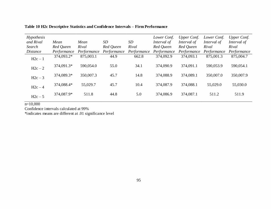
95
Table 10 H2c Descriptive Statistics and Confidence Intervals – Firm Performance
Hypothesis
and Rival
Search
Distance
Mean
Red Queen
Performance
Mean
Rival
Performance
SD
Red Queen
Performance
SD
Rival
Performance
Lower Conf.
Interval of
Red Queen
Performance
Upper Conf.
Interval of
Red Queen
Performance
Lower Conf.
Interval of
Rival
Performance
Upper Conf.
Interval of
Rival
Performance
H2c – 1 374,093.2* 875,003.1 44.9 662.8 374,092.9 374,093.1 875,001.3 875,004.7
H2c – 2 374,091.3* 590,054.0 55.0 34.1 374,090.9 374,091.1 590,053.9 590,054.1
H2c – 3 374,089.3* 350,007.3 45.7 14.8 374,088.9 374,089.1 350,007.0 350,007.9
H2c – 4 374,088.4* 55,029.7 45.7 10.4 374,087.9 374,088.1 55,029.0 55,030.0
H2c – 5 374,087.9* 511.8 44.8 5.0 374,086.9 374,087.1 511.2 511.9
n=10,000
Confidence intervals calculated at 99%
*indicates means are different at .01 significance level
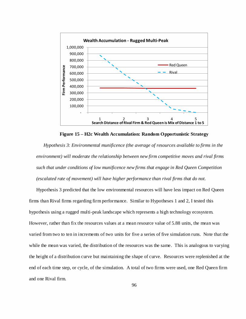
96
Figure 15 – H2c Wealth Accumulation: Random Opportunistic Strategy
Hypothesis 3: Environmental munificence (the average of resources available to firms in the
environment) will moderate the relationship between new firm competitive moves and rival firms
such that under conditions of low munificence new firms that engage in Red Queen Competition
(escalated rate of movement) will have higher performance than rival firms that do not.
Hypothesis 3 predicted that the low environmental resources will have less impact on Red Queen
firms than Rival firms regarding firm performance. Similar to Hypotheses 1 and 2, I tested this
hypothesis using a rugged multi-peak landscape which represents a high technology ecosystem.
However, rather than fix the resources values at a mean resource value of 5.88 units, the mean was
varied from two to ten in increments of two units for five a series of five simulation runs. Note that the
while the mean was varied, the distribution of the resources was the same. This is analogous to varying
the height of a distribution curve but maintaining the shape of curve. Resources were replenished at the
end of each time step, or cycle, of the simulation. A total of two firms were used, one Red Queen firm
and one Rival firm.
-
100,000
200,000
300,000
400,000
500,000
600,000
700,000
800,000
900,000
1,000,000
1 2 3 4 5
Firm
Pe
rfo
rman
ce
Search Distance of Rival Firm & Red Queen is Mix of Distance 1 to 5
Wealth Accumulation - Rugged Multi-Peak
Red Queen
Rival
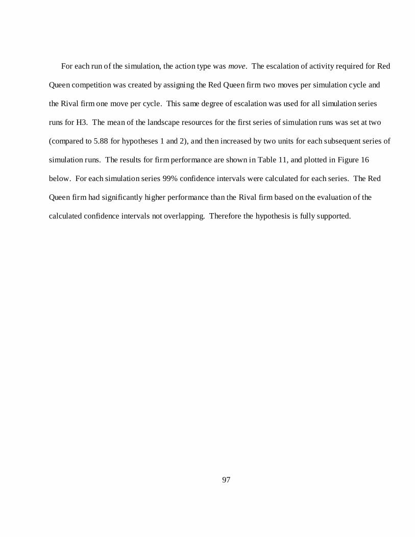
97
For each run of the simulation, the action type was move. The escalation of activity required for Red
Queen competition was created by assigning the Red Queen firm two moves per simulation cycle and
the Rival firm one move per cycle. This same degree of escalation was used for all simulation series
runs for H3. The mean of the landscape resources for the first series of simulation runs was set at two
(compared to 5.88 for hypotheses 1 and 2), and then increased by two units for each subsequent series of
simulation runs. The results for firm performance are shown in Table 11, and plotted in Figure 16
below. For each simulation series 99% confidence intervals were calculated for each series. The Red
Queen firm had significantly higher performance than the Rival firm based on the evaluation of the
calculated confidence intervals not overlapping. Therefore the hypothesis is fully supported.
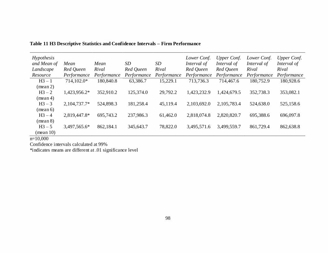
98
Table 11 H3 Descriptive Statistics and Confidence Intervals – Firm Performance
Hypothesis
and Mean of
Landscape
Resource
Mean
Red Queen
Performance
Mean
Rival
Performance
SD
Red Queen
Performance
SD
Rival
Performance
Lower Conf.
Interval of
Red Queen
Performance
Upper Conf.
Interval of
Red Queen
Performance
Lower Conf.
Interval of
Rival
Performance
Upper Conf.
Interval of
Rival
Performance
H3 – 1
(mean 2)
714,102.0* 180,840.8 63,386.7 15,229.1 713,736.3 714,467.6 180,752.9 180,928.6
H3 – 2
(mean 4)
1,423,956.2* 352,910.2 125,374.0 29,792.2 1,423,232.9 1,424,679.5 352,738.3 353,082.1
H3 – 3
(mean 6)
2,104,737.7* 524,898.3 181,258.4 45,119.4 2,103,692.0 2,105,783.4 524,638.0 525,158.6
H3 – 4
(mean 8)
2,819,447.8* 695,743.2 237,986.3 61,462.0 2,818,074.8 2,820,820.7 695,388.6 696,097.8
H3 – 5
(mean 10)
3,497,565.6* 862,184.1 345,643.7 78,822.0 3,495,571.6 3,499,559.7 861,729.4 862,638.8
n=10,000
Confidence intervals calculated at 99%
*indicates means are different at .01 significance level
99
Figure 16 - H3 Wealth Accumulation: Random Opportunistic Strategy
Hypotheses 4: Environmental dynamism (the variance of resources available to firms in the
environment) will moderate the relationship between firm search-distance for resources such that
under conditions of high dynamism (high variability), new firms that engage in Red Queen
Competition (escalated search-distance) will have better performance than new rival firms that do
not.
Hypothesis 4 predicted that the high environmental resource variance will have less impact on a Red
Queen firm‘s performance than on a Rival firm‘s performance. Similar to all the hypotheses tested so
far, I tested this hypothesis using a rugged multi-peak landscape which represents a high technology
ecosystem. For hypothesis 3 I varied the peak of the resource distribution curve and held the form of the
curve constant, but for hypothesis 4 I varied the shape of resource distribution curve and held the
average resource level constant.19 I created three different landscape maps to test hypothesis 4. Version
one, the base version, is the standard landscape map used for all other simulations, the rugged multi-
19 I suggest that this is an important point in the simulation configuration. Simply varying the shape of
the curve accomplished creating the variance in resource availability. However, if the resource average
is not maintained, it is difficult to determine the effect of the change in the distribution.
-
500,000
1,000,000
1,500,000
2,000,000
2,500,000
3,000,000
3,500,000
4,000,000
1 2 3 4 5
Firm
Pe
rfo
rman
ce
Landscape Resource Availability Mean Varies from 2 to 10
Wealth Accumulation on Rugged Multi-Peak Landscape
Red Queen
Rival
100
peak with a normal near linear distribution. Version two was created using a more rapidly declining
resource curve than the standard landscape. Version three was created using a more gradually declining
resource curve than the standard landscape. The resource curve shapes were depicted in chapter 3,
Figure 9. Resources were replenished at the end of each time step, or cycle, of the simulation. A total
of two firms were used, one Red Queen firm and one Rival firm.
For each run of the simulation, the action type was search-distance. The escalation of activity
required for Red Queen competition was created by assigning the Red Queen firm a search-distance of
two spaces and the Rival firm a search-distance of one space per cycle. Three series of simulation runs
were made of 10,000 simulations each, one series for each of the three resource distributions. For each
simulation series, based on the 99% confidence intervals shown in Table 12, the Red Queen firm had
significantly lower performance than the Rival firm. Therefore the hypothesis is not supported. The
means of firm performance are plotted in Figure 17.
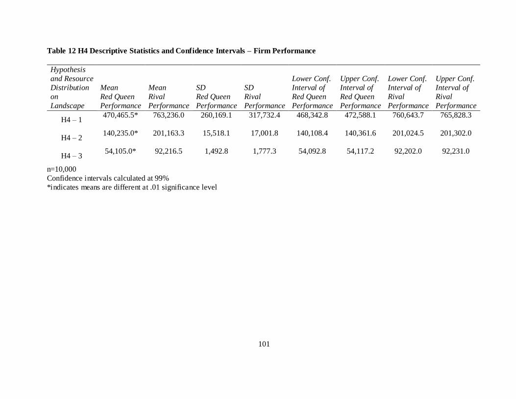
101
Table 12 H4 Descriptive Statistics and Confidence Intervals – Firm Performance
Hypothesis
and Resource
Distribution
on
Landscape
Mean
Red Queen
Performance
Mean
Rival
Performance
SD
Red Queen
Performance
SD
Rival
Performance
Lower Conf.
Interval of
Red Queen
Performance
Upper Conf.
Interval of
Red Queen
Performance
Lower Conf.
Interval of
Rival
Performance
Upper Conf.
Interval of
Rival
Performance
H4 – 1 470,465.5* 763,236.0 260,169.1 317,732.4 468,342.8 472,588.1 760,643.7 765,828.3
H4 – 2 140,235.0* 201,163.3 15,518.1 17,001.8 140,108.4 140,361.6 201,024.5 201,302.0
H4 – 3 54,105.0* 92,216.5 1,492.8 1,777.3 54,092.8 54,117.2 92,202.0 92,231.0
n=10,000
Confidence intervals calculated at 99%
*indicates means are different at .01 significance level
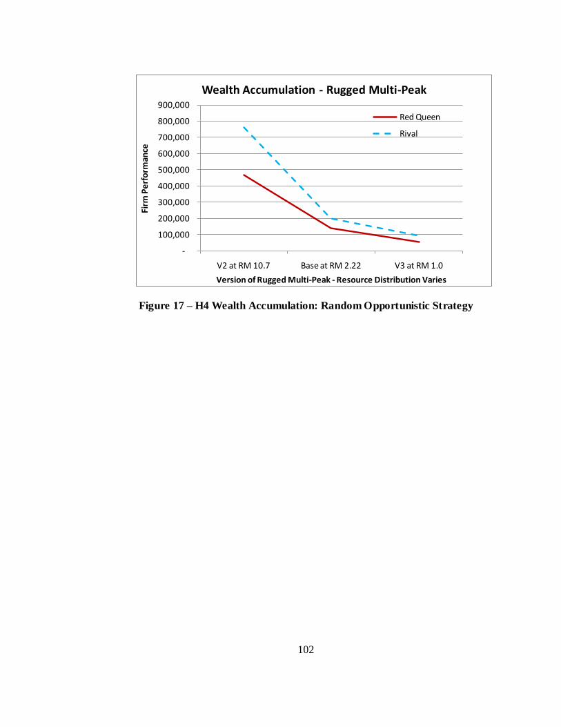
102
Figure 17 – H4 Wealth Accumulation: Random Opportunistic Strategy
-
100,000
200,000
300,000
400,000
500,000
600,000
700,000
800,000
900,000
V2 at RM 10.7 Base at RM 2.22 V3 at RM 1.0
Firm
Pe
rfo
rman
ce
Version of Rugged Multi-Peak - Resource Distribution Varies
Wealth Accumulation - Rugged Multi-Peak
Red Queen
Rival
103
CHAPTER 4: DISCUSSION Summary
The purpose of my dissertation was to develop and test a simulation model of Red Queen
competition that could be used to explore the Red Queen Effect on new firm performance and survival
in a high technology ecosystem. First, I developed a theoretical model of the essential components of
Red Queen competition and used this to explain how the kind of escalating competition leads to the Red
Queen Effect. Research questions were developed from this theoretical model to guide my exploration
of how activity escalation works as to really change the performance and survival of new firms. Using
the essentials from the theoretical model, I developed an agent-based model to create Red Queen
competition between firms. Predictions developed from the theoretical model were tested using data
collected from the simulation.
The results of the data collection provided support for about one half of the predictions and there
were a few revealing findings across the predictions. Overall, the results suggest that the Red Queen
Effect is both positive and negative on new firm performance and survival. Data on different types of
activity were collected and analyzed. The results indicate that the escalation of different types of
activities has different effects. This may shed light on why many empirical studies to-date on the Red
Queen Effect have mixed results. Further, data were collected on the impact on firms when there are
changes in environmental resources needed by the firms to survive. These results reveal the importance
of measuring and controlling for environmental resources to accurately measure the Red Queen Effect.
The remainder of this chapter focuses on a discussion of the results that emerge from the simulation data
collection.
Findings
Table 13 is a summary of the findings from the data collection.

104
Table 13 Summary of Hypotheses Testing
Hypothesis Landscape Action
type
Outcome of Interest Strategy Result
H1a Rugged Multi-
peak
Move Survival Random Opportunistic
Random Direction*
Not supported
Not supported
H1b Rugged Multi-
peak
Move Wealth
Accumulation
Random Opportunistic
Random Direction*
Partially supported
Supported
H2a Rugged Multi-
peak
Search
Distance
Survival Random Opportunistic
Random Direction*
Not Supported
Not supported
H2b Rugged Multi-
peak
Search
Distance
Wealth
Accumulation
Random Opportunistic
Random Direction*
Not supported
Not Supported
H2c Rugged Multi-
peak
Search
Distance
Wealth
Accumulation
Random Opportunistic
Random Direction*
Partially Supported
Partially Supported
H3 Rugged Multi-
peak
Move Wealth
Accumulation
Random Opportunistic
Random Direction*
Supported
Supported
H4 Rugged Multi-
peak
Search
Distance
Wealth
Accumulation
Random Opportunistic
Random Direction*
Not supported
Not Supported
*Not hypothesized as the theorized logic of competition/strategy to be tested, but included for discussion purposes.
105
Escalated Activity Related Findings
The activity-related hypotheses (H1a, H1b, H2a, H2b, and H2c) predicted that the relationship
between a new firm with escalated activity, referred to in my discussion as the Red Queen firm, and a
new rival firm, the Rival firm, would have a higher survival rate and higher performance on the part of
the Red Queen firm. The factor that I thought would enhance the survival and performance of the Red
Queen firm was the escalated activity on the part of the Red Queen firm.
The logic behind the idea that the escalated activity level would positively affect this relationship
was based on assertions put forth in the Red Queen Effect Theory. This theory is based on the work in
field of biology by van Valen (1973), in the field of economics by Baumol (2004), and in the field of
strategic management by Barnett (1989, 1993, 1997, and 2008). There research suggests that firms
engage in competition with each other to learn about the logic of competition of the firms. The firms
also engage in competition to learn about the landscape that they are competing upon. Through this
learning the firm adapts to the advantage of the firm, and this leads to the increased survival and
performance. However, the results of the activity-based hypotheses provide mixed findings with regard
to this expectation.
Hypothesis 1a tested the relationship between escalated move-based activities among competing
firms on firm survival. The firm designated the Red Queen firm moved an escalated number of spaces
on the landscape relative to the firm designated the Rival firm as the firms competed for resources. The
resources were distributed on a landscape that was created to mimic a high technology environment.
The environment was termed a rugged multi-peak landscape, and it was designed to be difficult for
firms to navigate, and difficult for firms to find a pattern of resource allocation on the landscape due to
the seemingly ever changing peaks and valleys on they encountered. The predicted results for this
hypothesis were not supported.
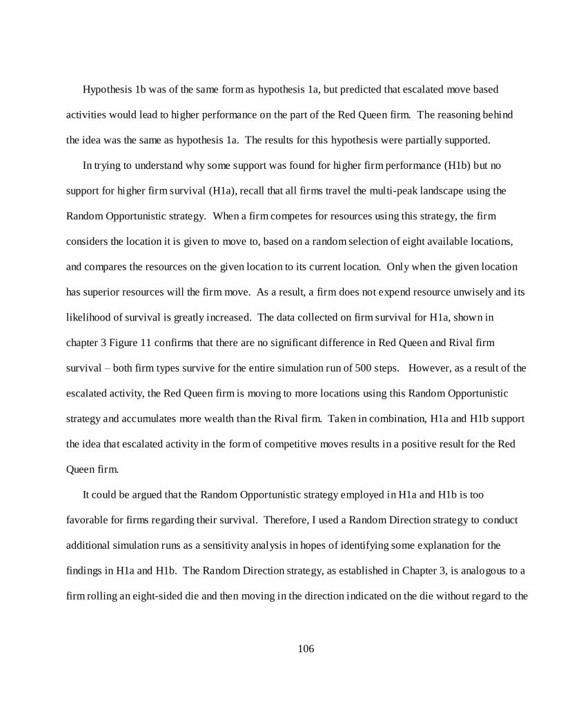
106
Hypothesis 1b was of the same form as hypothesis 1a, but predicted that escalated move based
activities would lead to higher performance on the part of the Red Queen firm. The reasoning behind
the idea was the same as hypothesis 1a. The results for this hypothesis were partially supported.
In trying to understand why some support was found for higher firm performance (H1b) but no
support for higher firm survival (H1a), recall that all firms travel the multi-peak landscape using the
Random Opportunistic strategy. When a firm competes for resources using this strategy, the firm
considers the location it is given to move to, based on a random selection of eight available locations,
and compares the resources on the given location to its current location. Only when the given location
has superior resources will the firm move. As a result, a firm does not expend resource unwisely and its
likelihood of survival is greatly increased. The data collected on firm survival for H1a, shown in
chapter 3 Figure 11 confirms that there are no significant difference in Red Queen and Rival firm
survival – both firm types survive for the entire simulation run of 500 steps. However, as a result of the
escalated activity, the Red Queen firm is moving to more locations using this Random Opportunistic
strategy and accumulates more wealth than the Rival firm. Taken in combination, H1a and H1b support
the idea that escalated activity in the form of competitive moves results in a positive result for the Red
Queen firm.
It could be argued that the Random Opportunistic strategy employed in H1a and H1b is too
favorable for firms regarding their survival. Therefore, I used a Random Direction strategy to conduct
additional simulation runs as a sensitivity analysis in hopes of identifying some explanation for the
findings in H1a and H1b. The Random Direction strategy, as established in Chapter 3, is analogous to a
firm rolling an eight-sided die and then moving in the direction indicated on the die without regard to the
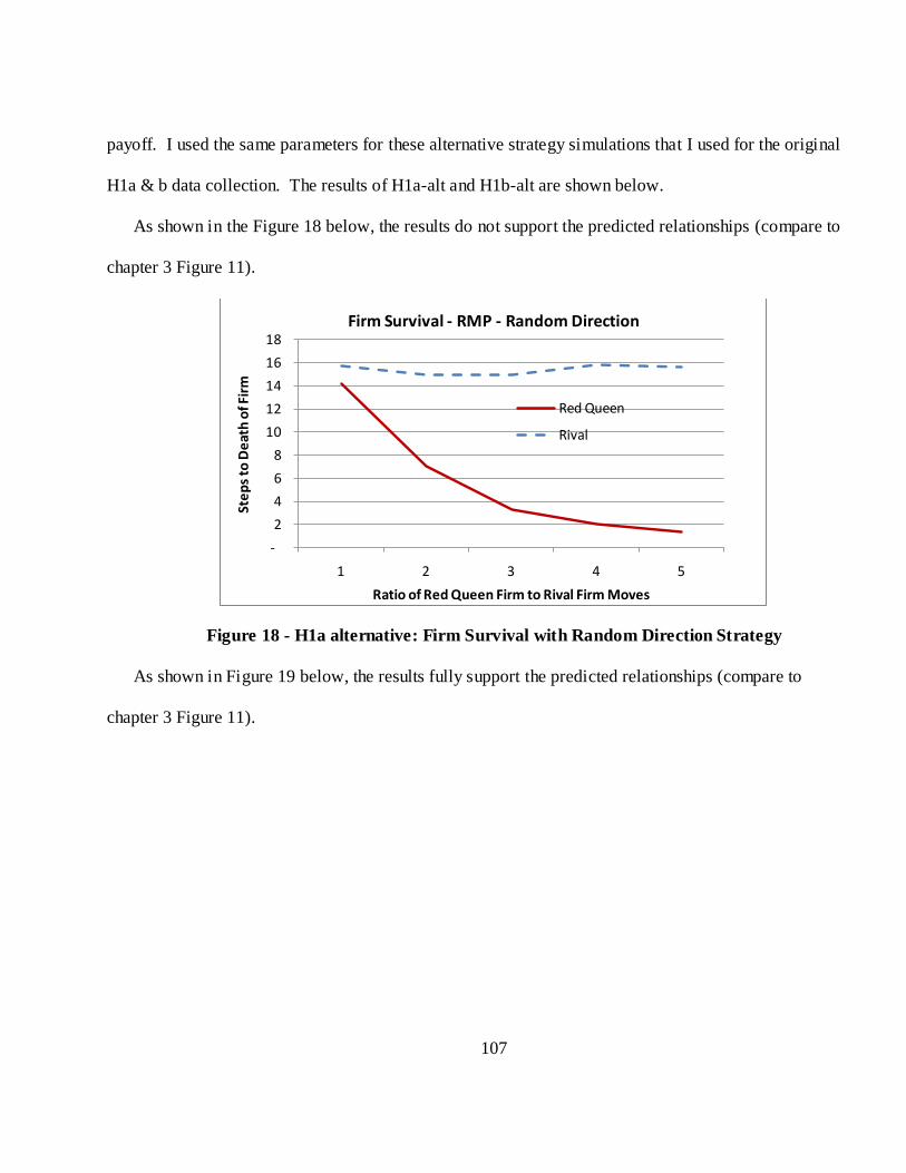
107
payoff. I used the same parameters for these alternative strategy simulations that I used for the original
H1a & b data collection. The results of H1a-alt and H1b-alt are shown below.
As shown in the Figure 18 below, the results do not support the predicted relationships (compare to
chapter 3 Figure 11).
Figure 18 - H1a alternative: Firm Survival with Random Direction Strategy
As shown in Figure 19 below, the results fully support the predicted relationships (compare to
chapter 3 Figure 11).
-
2
4
6
8
10
12
14
16
18
1 2 3 4 5
Ste
ps
to D
eat
h o
f Fir
m
Ratio of Red Queen Firm to Rival Firm Moves
Firm Survival - RMP - Random Direction
Red Queen
Rival
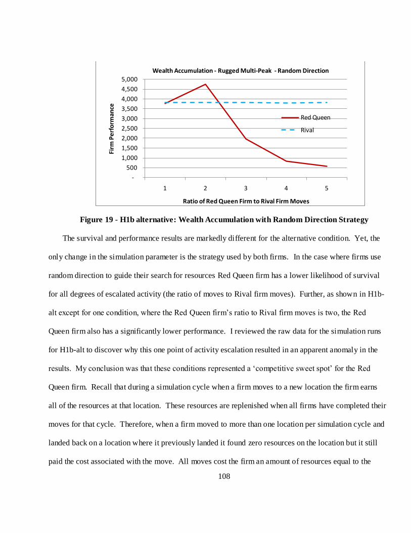
108
Figure 19 - H1b alternative: Wealth Accumulation with Random Direction Strategy
The survival and performance results are markedly different for the alternative condition. Yet, the
only change in the simulation parameter is the strategy used by both firms. In the case where firms use
random direction to guide their search for resources Red Queen firm has a lower likelihood of survival
for all degrees of escalated activity (the ratio of moves to Rival firm moves). Further, as shown in H1b-
alt except for one condition, where the Red Queen firm‘s ratio to Rival firm moves is two, the Red
Queen firm also has a significantly lower performance. I reviewed the raw data for the simulation runs
for H1b-alt to discover why this one point of activity escalation resulted in an apparent anomaly in the
results. My conclusion was that these conditions represented a ‗competitive sweet spot‘ for the Red
Queen firm. Recall that during a simulation cycle when a firm moves to a new location the firm earns
all of the resources at that location. These resources are replenished when all firms have completed their
moves for that cycle. Therefore, when a firm moved to more than one location per simulation cycle and
landed back on a location where it previously landed it found zero resources on the location but it still
paid the cost associated with the move. All moves cost the firm an amount of resources equal to the
-
500
1,000
1,500
2,000
2,500
3,000
3,500
4,000
4,500
5,000
1 2 3 4 5
Firm
Pe
rfo
rman
ce
Ratio of Red Queen Firm to Rival Firm Moves
Wealth Accumulation - Rugged Multi-Peak - Random Direction
Red Queen
Rival
109
average amount of resources on the landscape. The likelihood of a firm landing on a location with zero
resources increased as the firm continued to escalate the number of moves the firm makes per simulation
cycle. A Red Queen firm that moved two locations per cycle was the optimal for the given set of
conditions used in all the simulations20.
I believe this provides some clear insight into why some empirical studies have concluded with
mixed results. Although the conditions for Red Queen competition were met for both the original and
the alternative conditions tested, the competitive strategy used by the firms, random opportunistic or
random direction, had a profound difference on the predicted outcomes. The requirement to explicitly
identify the strategy of the firm is a requirement of Red Queen competition that is rarely if ever upheld
in empirical research. Yet it is part of one of Barnett‘s (2008) conditions noted in chapter 2, referred to
as how the firms compete, specifically their logic of competition.
Hypotheses 2a and 2b examined the impact of escalated search activity on firm survival and
performance using the search activity mode rather than the move activity mode that was used in
hypotheses 1a and 1b. The firm designated the Red Queen firm moved an escalated number of spaces
on the landscape compared to the firm designated the Rival firm as the firms competed for resources.
Where the firms moved on contiguous spaces on the landscape in H1a and H1b, the firms jumped or
leaped a distance from their current location equal to the search-distance they were given for their
simulation run. As with H1a and H1b, the resources were distributed on a landscape that was created to
mimic a high technology environment. The environment was termed a rugged multi-peak landscape,
and it was designed to be difficult for firms to navigate and difficult for firms to find a pattern of
20 I was able to further confirm this by an additional variant of the simulation where I set the cost to
move to zero. In this test case the results for firm survival and firm performance were not significantly
different.
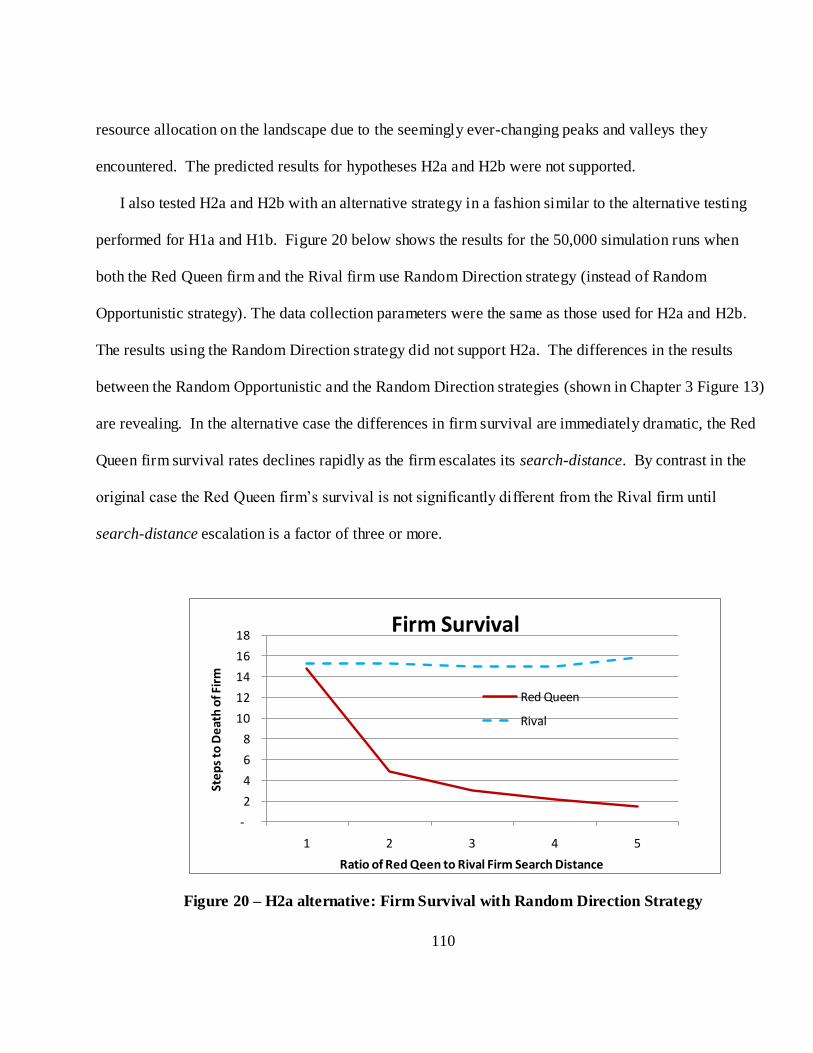
110
resource allocation on the landscape due to the seemingly ever-changing peaks and valleys they
encountered. The predicted results for hypotheses H2a and H2b were not supported.
I also tested H2a and H2b with an alternative strategy in a fashion similar to the alternative testing
performed for H1a and H1b. Figure 20 below shows the results for the 50,000 simulation runs when
both the Red Queen firm and the Rival firm use Random Direction strategy (instead of Random
Opportunistic strategy). The data collection parameters were the same as those used for H2a and H2b.
The results using the Random Direction strategy did not support H2a. The differences in the results
between the Random Opportunistic and the Random Direction strategies (shown in Chapter 3 Figure 13)
are revealing. In the alternative case the differences in firm survival are immediately dramatic, the Red
Queen firm survival rates declines rapidly as the firm escalates its search-distance. By contrast in the
original case the Red Queen firm‘s survival is not significantly different from the Rival firm until
search-distance escalation is a factor of three or more.
Figure 20 – H2a alternative: Firm Survival with Random Direction Strategy
-
2
4
6
8
10
12
14
16
18
1 2 3 4 5
Ste
ps
to D
eat
h o
f Fir
m
Ratio of Red Qeen to Rival Firm Search Distance
Firm Survival
Red Queen
Rival
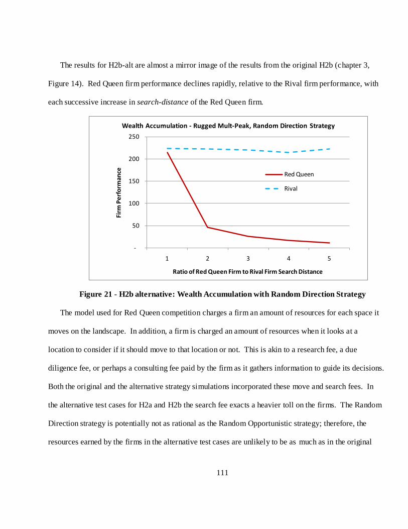
111
The results for H2b-alt are almost a mirror image of the results from the original H2b (chapter 3,
Figure 14). Red Queen firm performance declines rapidly, relative to the Rival firm performance, with
each successive increase in search-distance of the Red Queen firm.
Figure 21 - H2b alternative: Wealth Accumulation with Random Direction Strategy
The model used for Red Queen competition charges a firm an amount of resources for each space it
moves on the landscape. In addition, a firm is charged an amount of resources when it looks at a
location to consider if it should move to that location or not. This is akin to a research fee, a due
diligence fee, or perhaps a consulting fee paid by the firm as it gathers information to guide its decisions.
Both the original and the alternative strategy simulations incorporated these move and search fees. In
the alternative test cases for H2a and H2b the search fee exacts a heavier toll on the firms. The Random
Direction strategy is potentially not as rational as the Random Opportunistic strategy; therefore, the
resources earned by the firms in the alternative test cases are unlikely to be as much as in the original
-
50
100
150
200
250
1 2 3 4 5
Firm
Pe
rfo
rman
ce
Ratio of Red Queen Firm to Rival Firm Search Distance
Wealth Accumulation - Rugged Mult-Peak, Random Direction Strategy
Red Queen
Rival
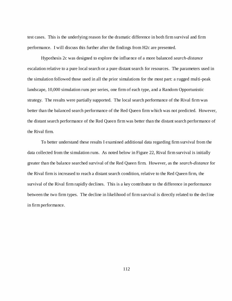
112
test cases. This is the underlying reason for the dramatic difference in both firm survival and firm
performance. I will discuss this further after the findings from H2c are presented.
Hypothesis 2c was designed to explore the influence of a more balanced search-distance
escalation relative to a pure local search or a pure distant search for resources. The parameters used in
the simulation followed those used in all the prior simulations for the most part: a rugged multi-peak
landscape, 10,000 simulation runs per series, one firm of each type, and a Random Opportunistic
strategy. The results were partially supported. The local search performance of the Rival firm was
better than the balanced search performance of the Red Queen firm which was not predicted. However,
the distant search performance of the Red Queen firm was better than the distant search performance of
the Rival firm.
To better understand these results I examined additional data regarding firm survival from the
data collected from the simulation runs. As noted below in Figure 22, Rival firm survival is initially
greater than the balance searched survival of the Red Queen firm. However, as the search-distance for
the Rival firm is increased to reach a distant search condition, relative to the Red Queen firm, the
survival of the Rival firm rapidly declines. This is a key contributor to the difference in performance
between the two firm types. The decline in likelihood of firm survival is directly related to the decl ine
in firm performance.
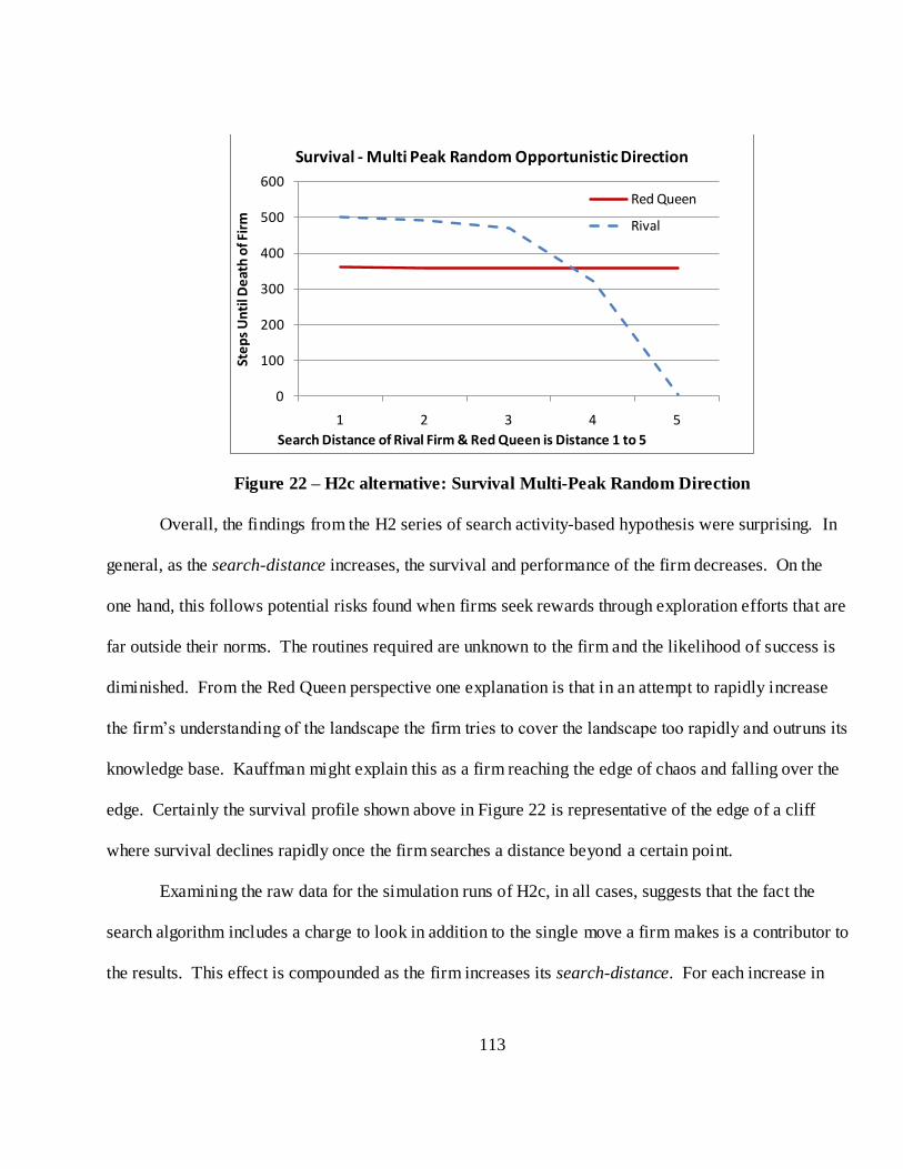
113
Figure 22 – H2c alternative: Survival Multi-Peak Random Direction
Overall, the findings from the H2 series of search activity-based hypothesis were surprising. In
general, as the search-distance increases, the survival and performance of the firm decreases. On the
one hand, this follows potential risks found when firms seek rewards through exploration efforts that are
far outside their norms. The routines required are unknown to the firm and the likelihood of success is
diminished. From the Red Queen perspective one explanation is that in an attempt to rapidly increase
the firm‘s understanding of the landscape the firm tries to cover the landscape too rapidly and outruns its
knowledge base. Kauffman might explain this as a firm reaching the edge of chaos and falling over the
edge. Certainly the survival profile shown above in Figure 22 is representative of the edge of a cliff
where survival declines rapidly once the firm searches a distance beyond a certain point.
Examining the raw data for the simulation runs of H2c, in all cases, suggests that the fact the
search algorithm includes a charge to look in addition to the single move a firm makes is a contributor to
the results. This effect is compounded as the firm increases its search-distance. For each increase in
0
100
200
300
400
500
600
1 2 3 4 5
Ste
ps
Un
til D
eat
h o
f Fir
m
Search Distance of Rival Firm & Red Queen is Distance 1 to 5
Survival - Multi Peak Random Opportunistic Direction
Red Queen
Rival
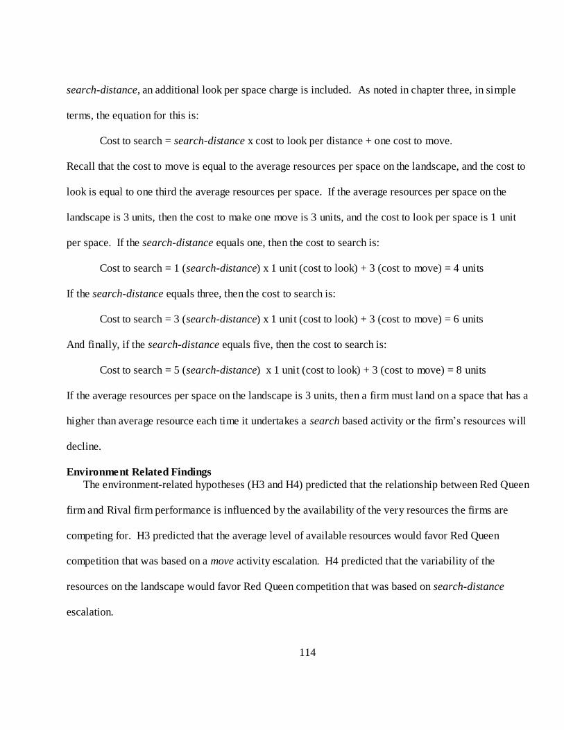
114
search-distance, an additional look per space charge is included. As noted in chapter three, in simple
terms, the equation for this is:
Cost to search = search-distance x cost to look per distance + one cost to move.
Recall that the cost to move is equal to the average resources per space on the landscape, and the cost to
look is equal to one third the average resources per space. If the average resources per space on the
landscape is 3 units, then the cost to make one move is 3 units, and the cost to look per space is 1 unit
per space. If the search-distance equals one, then the cost to search is:
Cost to search = 1 (search-distance) x 1 unit (cost to look) + 3 (cost to move) = 4 units
If the search-distance equals three, then the cost to search is:
Cost to search = 3 (search-distance) x 1 unit (cost to look) + 3 (cost to move) = 6 units
And finally, if the search-distance equals five, then the cost to search is:
Cost to search = 5 (search-distance) x 1 unit (cost to look) + 3 (cost to move) = 8 units
If the average resources per space on the landscape is 3 units, then a firm must land on a space that has a
higher than average resource each time it undertakes a search based activity or the firm‘s resources will
decline.
Environment Related Findings
The environment-related hypotheses (H3 and H4) predicted that the relationship between Red Queen
firm and Rival firm performance is influenced by the availability of the very resources the firms are
competing for. H3 predicted that the average level of available resources would favor Red Queen
competition that was based on a move activity escalation. H4 predicted that the variability of the
resources on the landscape would favor Red Queen competition that was based on search-distance
escalation.

115
As noted earlier, the logic behind the idea that the escalated activity level would positively affect this
relationship was based on assertions put forth in the Red Queen Effect Theory. I model two different
types of activity for my simulations, move and search-distance. Note that I associated move based
activity with H3 and search-distance activity with H4.
H3 tests the effect of Red Queen competition on five different multi-peak environment landscapes
with a uniform distribution of resources on each of the peaks21 on each of the three landscapes. The
average of the resources on the five landscapes was varied by changing the mean of the resource curve
but not the shape of the distribution of resources about this mean. Changing the mean of the resources
while holding the distribution the same translates into a change in the total resources available to firms
as they compete for resources. The results for H3 were that a Red Queen firm that used an escalated
move based activity achieved higher performance results. Therefore, the prediction for H3 was
supported.
Although not hypothesized, I performed additional post-hoc analysis to gain insight into why the
Red Queen firm perspective was supported in H3. I again used an alternate competitive logic strategy
and substituted Random Direction for the originally used Random Opportunistic strategy in a series of
simulation runs. All other parameters of the H3 data collection were kept the same. The results show
the impact – the alternate hypothesis H3-alt is not supported. The escalated move strategy does not
significantly improve the accumulation of wealth for the Red Queen firm. This finding once again sheds
light on why prior research in the Red Queen Effect may have reached mixed conclusions.
21 Per prior discussions, the multi-peak landscape is based on four peaks with each of the four peaks
differs in resource height such that there are four different heights with one of the heights offering the
greatest amount of resources at its peak.
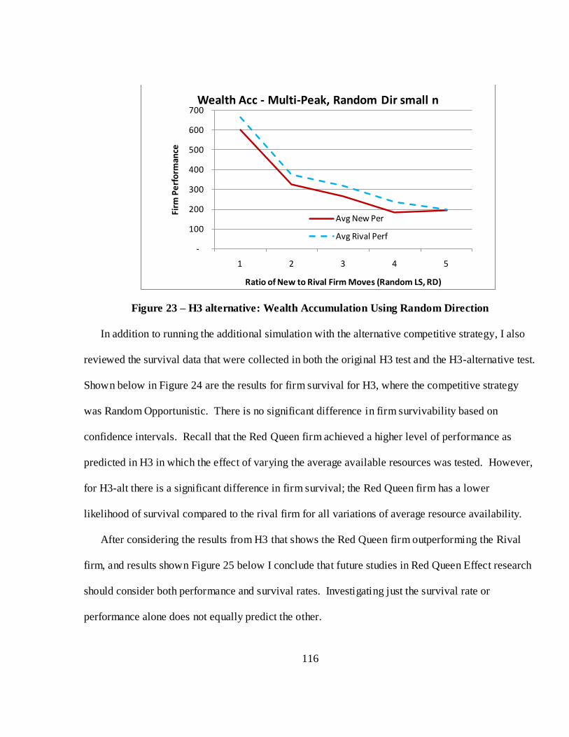
116
Figure 23 – H3 alternative: Wealth Accumulation Using Random Direction
In addition to running the additional simulation with the alternative competitive strategy, I also
reviewed the survival data that were collected in both the original H3 test and the H3-alternative test.
Shown below in Figure 24 are the results for firm survival for H3, where the competitive strategy
was Random Opportunistic. There is no significant difference in firm survivability based on
confidence intervals. Recall that the Red Queen firm achieved a higher level of performance as
predicted in H3 in which the effect of varying the average available resources was tested. However,
for H3-alt there is a significant difference in firm survival; the Red Queen firm has a lower
likelihood of survival compared to the rival firm for all variations of average resource availability.
After considering the results from H3 that shows the Red Queen firm outperforming the Rival
firm, and results shown Figure 25 below I conclude that future studies in Red Queen Effect research
should consider both performance and survival rates. Investigating just the survival rate or
performance alone does not equally predict the other.
-
100
200
300
400
500
600
700
1 2 3 4 5
Firm
Pe
rfo
rman
ce
Ratio of New to Rival Firm Moves (Random LS, RD)
Wealth Acc - Multi-Peak, Random Dir small n
Avg New Per
Avg Rival Perf
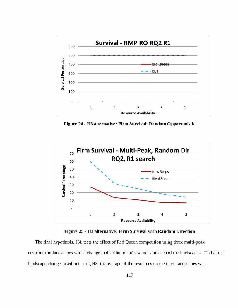
117
Figure 24 - H3 alternative: Firm Survival: Random Opportunistic
Figure 25 - H3 alternative: Firm Survival with Random Direction
The final hypothesis, H4, tests the effect of Red Queen competition using three multi-peak
environment landscapes with a change in distribution of resources on each of the landscapes. Unlike the
landscape changes used in testing H3, the average of the resources on the three landscapes was
-
100
200
300
400
500
600
1 2 3 4 5
Surv
ival
Pe
rce
nta
ge
Resource Availability
Survival - RMP RO RQ2 R1
Red Queen
Rival
-
10
20
30
40
50
60
70
1 2 3 4 5
Surv
ival
Pe
rce
nta
ge
Resource Availability
Firm Survival - Multi-Peak, Random Dir RQ2, R1 search
New Steps
Rival Steps
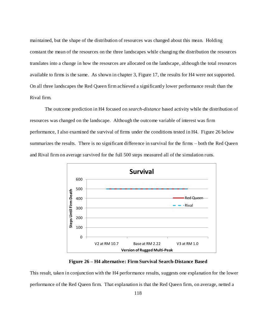
118
maintained, but the shape of the distribution of resources was changed about this mean. Holding
constant the mean of the resources on the three landscapes while changing the distribution the resources
translates into a change in how the resources are allocated on the landscape, although the total resources
available to firms is the same. As shown in chapter 3, Figure 17, the results for H4 were not supported.
On all three landscapes the Red Queen firm achieved a significantly lower performance result than the
Rival firm.
The outcome prediction in H4 focused on search-distance based activity while the distribution of
resources was changed on the landscape. Although the outcome variable of interest was firm
performance, I also examined the survival of firms under the conditions tested in H4. Figure 26 below
summarizes the results. There is no significant difference in survival for the firms – both the Red Queen
and Rival firm on average survived for the full 500 steps measured all of the simulation runs.
Figure 26 – H4 alternative: Firm Survival Search-Distance Based
This result, taken in conjunction with the H4 performance results, suggests one explanation for the lower
performance of the Red Queen firm. That explanation is that the Red Queen firm, on average, netted a
0
100
200
300
400
500
600
V2 at RM 10.7 Base at RM 2.22 V3 at RM 1.0
Ste
ps
Un
til F
irm
De
ath
Version of Rugged Multi-Peak
Survival
Red Queen
Rival
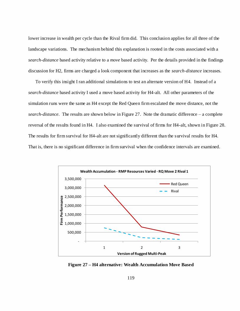
119
lower increase in wealth per cycle than the Rival firm did. This conclusion applies for all three of the
landscape variations. The mechanism behind this explanation is rooted in the costs associated with a
search-distance based activity relative to a move based activity. Per the details provided in the findings
discussion for H2, firms are charged a look component that increases as the search-distance increases.
To verify this insight I ran additional simulations to test an alternate version of H4. Instead of a
search-distance based activity I used a move based activity for H4-alt. All other parameters of the
simulation runs were the same as H4 except the Red Queen firm escalated the move distance, not the
search-distance. The results are shown below in Figure 27. Note the dramatic difference – a complete
reversal of the results found in H4. I also examined the survival of firms for H4-alt, shown in Figure 28.
The results for firm survival for H4-alt are not significantly different than the survival results for H4.
That is, there is no significant difference in firm survival when the confidence intervals are examined.
Figure 27 – H4 alternative: Wealth Accumulation Move Based
-
500,000
1,000,000
1,500,000
2,000,000
2,500,000
3,000,000
3,500,000
1 2 3
Firm
Pe
rfo
rman
ce
Version of Rugged Multi-Peak
Wealth Accumulation - RMP Resources Varied - RQ Move 2 Rival 1
Red Queen
Rival
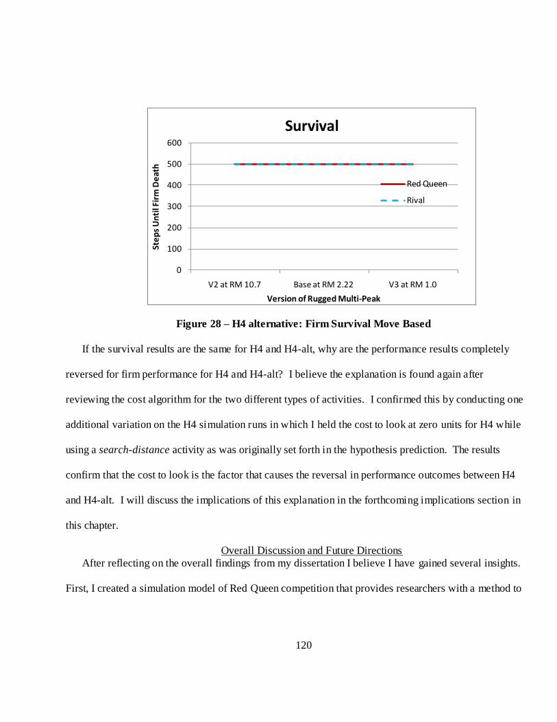
120
Figure 28 – H4 alternative: Firm Survival Move Based
If the survival results are the same for H4 and H4-alt, why are the performance results completely
reversed for firm performance for H4 and H4-alt? I believe the explanation is found again after
reviewing the cost algorithm for the two different types of activities. I confirmed this by conducting one
additional variation on the H4 simulation runs in which I held the cost to look at zero units for H4 while
using a search-distance activity as was originally set forth in the hypothesis prediction. The results
confirm that the cost to look is the factor that causes the reversal in performance outcomes between H4
and H4-alt. I will discuss the implications of this explanation in the forthcoming implications section in
this chapter.
Overall Discussion and Future Directions
After reflecting on the overall findings from my dissertation I believe I have gained several insights.
First, I created a simulation model of Red Queen competition that provides researchers with a method to
0
100
200
300
400
500
600
V2 at RM 10.7 Base at RM 2.22 V3 at RM 1.0
Ste
ps
Un
til F
irm
De
ath
Version of Rugged Multi-Peak
Survival
Red Queen
Rival
121
collect data and examine the Red Queen Effect that in turn improves how we do research on this
phenomenon. I list this point first because overall I believe it is the most significant point.
This point was made salient when I attended a panel discussion on modeling capabilities and the
RBV22 at the August 9, 2010 Academy of Management Conference in Montreal, Canada. The panel was
conducted by leading researchers in our domain: Ron Adner, Michael Jacobides, Dan Levinthal, Jan
Rivkin, and Sid Winter. Each researcher presented his reasons on why modeling should and could be
used to further our understanding of why studies of the RBV has perpetually resulted in mixed findings.
To a person, the panel members made two very bold statements. The first was that formal modeling and
simulation was the only way to untangle the value of the RBV by finding the conditions under which it
actually holds true. The second statement was that formal modeling and simulation have the potential to
be the next big breakthrough in management research. My experience with this dissertation research,
while certainly limited compared to the researchers on this panel, supports the second statement 23. The
key is the benefits of the precision in thought that model preparation forces in regard to the research
question under consideration.
As shown in my results section, the type of activity chosen does matter. Or, put another way, all
activities are not created equal in their impact on firm survival and performance. However, most of the
empirical studies treated all activities without regard to scale or intensity of the various types of
activities. New product introductions were combined with a change in price on existing products.
Further, little regard was given to the cost of activities. The implications seemed to be that all activity
types are uniform in their cost basis. As I discovered, the choice of how costs are charged to a firm
22 The Resource Based View, as commonly attributed to Barney (1991) and Wernerfelt (1984). 23 I cited the reasons given for this statement in Chapter Two (Jacobides and Winter, 2010).
122
relative to activity types can reverse the expected outcome of a predicted relationship. For the future
this suggests that the work put into developing models may hold great reward for management research.
As a note to balance this point, the precision required by quality modeling is time-consuming. It is not a
casual endeavor. In fact, my experience is that developing a precise specification, and then developing
the model, and then collecting data from the simulation runs using the model is more time-consuming
and labor intensive than any survey or secondary data collection with which I have been involved in.
This is due in part to this being my first effort in this area. But I believe it also reflects the difficulty of
the task.
The second main point is that the Red Queen Effect can be either positive or negative on new firm
survival and performance depending on how the research is conducted. The sign of the effect, whether
positive or negative, can change based on some very simple issues that may be missed if the researcher
is too in the formulation of the research question or operationalization of key variables. I believe a clear
example of this was shown in my findings in the alternative hypothesis testing when the firm strategy
was changed from Random Opportunistic to Random Direction. In the simulation this represented using
a different algorithm for the firm when it came time to choose whether or not to move in the direction
the firm was given to take its action. I believe Barnett would classify this as the degree of intended
rationality exhibited by the firm. Random Direction is a more limited rationality than Random
Opportunistic. And yet the impact on the results was dramatic. This suggests that future empirical
research needs to consider the logic of competition that each firm uses and to be explicit about how it is
determined. It also suggests that future models of Red Queen competition should develop finer grained
algorithms regarding their logic of competition.
123
The third point is meaningful Red Queen Effect research requires paying very close attention to the
essentials of Red Queen competition. Van Valen (1973), Baumol (2004) and Barnett (1989, 1993) were
clear enough in their early work to spell out what constitutes Red Queen competition. It is a necessary
condition for the Red Queen Effect to be observed. To be specific about this point, very few of the
empirical studies that I reviewed as part of my background preparation took the time to establish, or
report, that the firms they collected data on were in fact involved in competition that qualified as Red
Queen competition. A future direction for this line of research to be meaningful is that researchers
should take the care to collect variables that can be used to establish that the necessary conditions have
been met before they declare the Effect is present.
A fourth point is that context matters (Donaldson, 2001)24. Hypotheses 3 and 4 demonstrated that in
the case of resource availability and distribution the survival and performance of firms could be
significantly impacted. Some consideration for these environmental conditions has been attempted in
the empirical research to-date. Isolating the effect of environmental conditions might change some of
the mixed results from prior studies. For future research, salient environmental conditions should be
considered as moderators, and at some point controlled for.
Finally, the fundamental model of Red Queen research I created needs to be expanded to explore a
richer set of predictions. The results from the model I constructed provide baseline results. The model,
therefore, provides a way to examine the basic concepts of Red Queen research. That is, it addressed the
question of whether an escalation in competitive activity on the part of one firm, relative to a rival firm,
affects that firm‘s survival and performance. From the results I found, I believe the answer is yes, it
24 One of Dr. Marshall Schminke‘s teaching points in my organization theory seminar. Drawn from the
work of Donaldson (2001), Schminke regularly drew our attention to the contingencies in relationships,
and the importance of understanding the influence of moderators.
124
does. The results also provide insight into the areas of parameter sensitivity when conducting future
modeling or empirical research.
For example, I believe one future direction for Red Queen modeling is to explore the limits of the
Red Queen Effect. Another direction is to investigate the most likely types of interaction with other firm
and environmental conditions that influence the Effect. For instance, March (1991) and Kauffman
(1993) approached several related phenomena from their own different perspectives that may have the
Red Queen Effect at their center. One phenomenon is termed organizational learning by March, and I
suggest this is similar to what Kauffman termed species adaptation. March used a stochastic model to
explore how an individual‘s speed of learning influenced organizational learning. March also suggested
that local optima affect organizational learning. Kauffman used a fitness landscape structured model to
explore how adaptation affects survival and performance. He also suggested that local optima played a
role in limiting adaptation. And he suggested that there is a limit to the speed of adaptation, that if it is
exceeded it results in chaos.
One future modification to the model would be to include an explicit learning mode for each firm. I
envision a fast learning mode that would be implemented by firms being able to access the resource
information from the last five moves on a location by location basis, but they would be limited to this
fixed number of locations that the learn. A slow learning mode would delay the availability of the
information for some number of simulation cycles, say three to five, but once that passed the firm would
have total recall of all prior locations and resources. This would represent what March (1991) referred
to as a slow but deep learning of the organization. The firms would incorporate this knowledge of the
landscape into their competitive logic so that they could choose whether to move forward to new
locations or to return to an area that held more resources.
125
Another untapped area to be explored is the opposite side of Red Queen competition, or what I term
Red Queen cooperation. While Red Queen competition has been called an arms race, Red Queen
competition could be a peace race, or a cooperation race. This concept certainly borrows from the
prisoners‘ dilemma (Axelrod, 1997) but clearly extends it with the notion of escalation, not just
adaptation. Cooperation would open the theoretical model to resource sharing, resource trading, and
alliances.
The positive side of the Red Queen Effect is that if firms face fierce competitive rivalry and survive
it, they should be more fit in the long-run. This is due to what they have learned. It reflects the
adaptation of the firm to rivals and the environment. The negative side is that if firms attempt to adapt
too quickly they may burn unnecessary resources or may become maladaptive and suffer. We don‘t yet
know all of these boundary conditions. We also don‘t know how to effectively guide Red Queen
competition to be negative or positive. And we also don‘t know how to effectively regulate Red Queen
competition. Therefore, as noted in the above discussions, future direction should focus on developing a
more refined and more general Red Queen model to address these potential research areas.
Implications
Theoretical Implications
This dissertation offers contributions to work in entrepreneurship examining escalating competitive
rivalry as well as agent-based simulation model developed for management research. I developed a
theoretical model of Red Queen competition and used it to examine how escalations in activity-based
competition affect the survival and performance of new firms. I compared two different forms of
competitive activity, move based and search-distance based activity. Although the results of some of
the hypotheses were not supported, none of the results were inconclusive. I used post-hoc analysis,
typically based on additional simulation runs, to explore the unsupported hypotheses. This highlights
126
one significant contribution that simulation offers researchers over just empirical data – the ability to
explore the results in an experimental setting to find the causal mechanisms in relationships. In this
way, even if a hypothesis is not supported and explanation can be conclusively deduced.
The results of this study contribute to the stream of literature on the Red Queen Effect. One
contribution is made by confirming that the Red Queen Effect can be precisely modeled, and it can be
confirmed and disconfirmed. Using the model should allow researchers to examine the Red Queen
Effect at the edges25 and thereby improve construct definition and the understanding of boundary
conditions. In this same vein, it allows a parallel comparison with previous empirically based Red
Queen studies as a theoretical checklist to see if the studies met the requirements for Red Queen
competition, or were of the more general competitive dynamics form.
The other contribution is that the essential components of Red Queen competition, and the Red
Queen Effect, are explicitly defined. Further, they are operationalized in clear measurable terms and
defined by specific algorithms that make them repeatable. Using the model created for this study,
subsequent researchers will be able to modify the model to examine a richer set of conditions. Another
example is that although this model was created to focus on a special set of competitive dynamics
conditions, some of the constraints could be purposely relaxed to provide a model for general
competitive dynamics. This more general model could then be used to explore a wider range of
theoretical conditions that progressively develop from competitive dynamics, to Red Queen competition,
to the Red Queen Effect. Further, by including the resource boundary conditions available in the model
a researcher could develop theoretical test conditions to explore the conditions under which a firm
25 Per Kauffman (1993), the edge of chaos, or perhaps more generically considered tipping points or
conditions under which the Red Queen Effect can be found.

127
should engage in various degrees of competitive rivalry. I suggest that in all, these are significant
theoretical contributions.
Methodological Implications
This research also contributes to the methods research area of agent-based modeling in the domain
of management research. Agent-based modeling is relatively new to management research (Davis et al.,
2007; Gilbert, 2008) and very few examples exist to draw upon. As noted earlier, a detailed and
compelling discussion on the benefits of the methodology of simulation occurred at the Academy of
Management 2010 conference in a panel discussion on modeling (Jacobides et al., 2010). The panel
concluded that simulation may be the one method that offers objective insight into the conditions under
which the Resource Based View is valid. One reason is that simulation requires an objective delineation
of all of the critical constructs. The other reason is that the simulation offers complete control over the
interaction of the variables and the constructs.
The model that I created and used to collect data is based on these benefits of simulation. The
methodological implication is that I have implemented the Red Queen competition and therefore it can
be examined objectively. Further, per the guidelines established by Davis et al., (2007) the emerging
theory formed around Red Queen competition can be tested and modified in a controlled fashion. In a
sense, the simulation is a laboratory for Red Queen experimentation. Data can be collected rapidly
once the model is constructed and vetted. The implication here is rapid development of theory,
paralleling the concept of rapid prototype development in technology industries. One long term
implication is that the basic constructs of a theory can be modeled and simulated, and done so rapidly.
With the basic constructs modeled, and data are collected and analyzed, the more nuanced parts of the
theory can be examined by researchers using empirical data. In a sense, simulation will be a form of
automation for researchers.
128
I have included my specification for the entire model in Appendix B. I drew upon my background in
software project management to develop this specification. While it could be made more robust (and
longer believe it or not), I suggest that this specification provides a good framework for those who do
not have a background in software development to use. The specification should satisfy the guidelines
for simulation development from Davis et al., (2007) and Rand and Rust (2010).
In addition the NetLogo 4.1.1 simulation source code that I wrote, in its entirety, is included in
Appendix C. I have copyrighted this code with the usual disclaimers. This code allows a researcher to
jump-start his or her efforts in Red Queen competition research. It can also be used simply as an
example in a classroom environment on the subject of model and simulation development. And finally,
executing the program allows other researchers to verify my findings firsthand and then extend them if
they need to.
Practical Implications
Over the years that I worked on this dissertation I was often asked what I was doing my research on.
It took me some time to be able to explain this ‗as if I was talking to my grandmother,‘ as Dr. Rob
Folger26 would expect me to do. The practical implications are reflected in the answer that I give now
when asked about my research. This answer is along the lines of,
―There‘s an effect that biologists study called the Red Queen Effect. This effect happens
when one species escalates their competitive activities in response to another species in an
attempt to first survive and then to possibly outperform the rival species. They are competing for
the same resources in their environment. I am applying this interesting effect to new firms when
26 I had the privilege of taking several of my Ph.D. seminars from Rob and this was one of his regular
admonishments when we would get tongue tied over explaining theory.

129
these firms escalate their competitive activities with their rival firms. My findings are that the
Red Queen Effect is real, and it does make a difference. New firms need to make wise decisions
about how they compete with their rivals. Escalating their activity does not always work to their
advantage, and often leads to premature death of the firm.‖
Firms have choices regarding the type of action they take when they compete with other firms. In
conjunction with the type of action the firm chooses is the relative rate of the action. As shown in the
results, different types of actions and the associated degrees of activity escalation have widely different
results in firm survival and performance. Using just two types of action in this study, move based and
search-distance based, I demonstrated that not all actions have equal results. A new firm owner, or
manager, would be wise to carefully consider the type of action he or she chooses to either initiate
competition or to react to a rival competitor. The resources earned are directly correlated to the type of
action chosen.
Following the earning of resources, another practical implication is that new firm owners should
think through the costs of the actions they take when they compete with rival firms. As shown in the
different results between H1 and H2, the costs associated with escalating actions may quickly offset any
advantage gained. Red Queen competition is also referred to as an escalation of arms (Baumol, 2000).
The implication is similar to an escalation of commitment. Once a new firm owner starts down a path
he or she will continue regardless of the results. Instead, the findings of H1 and H2 strongly suggest that
the cost of actions be considered before taking the action, and that they be regularly evaluated.
One final practical implication is that the competitive context matters. Resource availability does
affect the results of a firm‘s competitive actions. I tested the effect of changing the average available
resources, and the distribution of resources. Changing the average a resource is akin to a macro level
130
change in the economy or across an entire industry. Changing the distribution is analogous to a change
in the concentration of resources, as occurs in market niches or customer groups. New firm managers,
therefore, need to stay apprised of their general or global environmental conditions, and also their
respect local conditions. This is often the last thing that a manager of a new technology startup takes
time to think about. Their primary goal is getting their new product to market. A corollary to this is that
something that worked in one marketplace with a given set of rival firms may not work in a different
marketplace competing against the same rival firms. Global or local conditions might not be similar
enough to allow the bridge or translation of actions to be as successful as they were in their original
environment.
Limitations
Although this study has a number of benefits, it also suffers from some limitations. Many of these
issues arise due to the implementation of the theoretical model of Red Queen competition as a
simulation model.
Perhaps the most important limitation is how I constructed the logic of competition used by each
firm. Barnett stipulates that firms engaged in Red Queen competition have intended rationality. Their
primary intentions are to take appropriate actions to survive. Beyond that, their intention is to improve
their performance to continue to survive in the future. My implementation is based on my extensive
consultations with a research biologist with first-hand knowledge of ecosystems (Dr. Betsy von Holle), a
computational evolutionist with a rich background in similar studies from a biological perspective (Dr.
Ivan Garibay), a recognized international authority on agent-based modeling with experience in Red
Queen models from the field of biology (Dr. William Rand), and my own experiences starting and
131
running several businesses. As noted in my post-hoc analysis, the choice of Random Direction27 or
Random Opportunistic28 strategy does affect several of the outcomes.
There are several limitations that arise from this implementation. First, I kept the firm strategy the
same for the entire series of simulation runs. My primary reason for doing this was to make the
interpretation of the results as straightforward as possible. However, it could be argued that most firms
would adjust their logic of competition during the battle with another firm. I kept the logic the same,
and used escalation of the number of moves or the search-distance as the part of the adaption required in
Red Queen competition. This limits the generalizability of the findings to firms that invoke just one
form of competitive logic for their entire life.
One consideration to address this limitation would be to vary the firm‘s competitive logic based on
the age of the firm, where the number of steps the firms has survived so far in the simulation is used as a
proxy for firm age. That is, all new firms, at birth, might start with a Random Direction strategy, and 50
cycles into the simulation this would be changed to Random Opportunistic.
Another consideration would be to vary the strategy based the outcomes of recent resource earnings
of the firm relative to rival firms. If all firms started with a Random Direction strategy, but one of the
firms continued to decline in accumulated wealth, that firm would change strategy to Random
Opportunistic. Or, the firm could change from a move based action to a search-distance based action.
This adds another level of complexity to the analysis, but it represents a more robust model.
27 Recall that Random Direction logic is when a firm randomly chooses a direction to move in from 360
degrees of options and moves without regard to the benefit or cost of the move. 28 Recall that Random Opportunistic logic is when a firm randomly chooses a direction to move in from
360 degrees of options, and then compares the resources that the firm will earn if it moves in this
direction relative to the resources it will earn if it stays in its current location for the cycle of the
simulation. The firm only moves when it is opportunistic for it to do so, or the resources are greater on
the location it randomly would move to.

132
Another potential limitation is the decision to charge a firm for each move, and each search-distance
the firm makes. First, the rational is based on the reality that firms do not undertake costless competitive
activities. Second, it is based on the precautions of Davis et al., (2007) regarding models being
unrealistic, particularly in this area of costless transactions. As noted in my post-hoc analysis, the
results in the search-distance based hypotheses are influenced by the imposed cost structure. However,
rather than try to optimize the model to achieve my desired predictions after I collected data, I designed
it to best reflect the real world prior to collecting data and I maintained the theoretical model. Note that
I did use a dynamic cost allocation algorithm in which the cost to move is set equal to the average cost of
resources on each location, and the cost to look in search-distance modes is one third of this, a more
sophisticated algorithm might yield more accurate results.
One consideration is to adjust the cost based on the age of the firm, or the size of the firm where
accumulated wealth is used as a proxy or the size of the firm. That is, as the firm ages, or grows larger
in size, the costs would be adjusted accordingly. A general adjustment would be that the costs are
increased with age and size. However, a more sophisticated adjustment could be made based on the
performance of the firm. A firm that makes efficient decisions might actually be given reduced costs
instead of increased costs. This would represent a form of learning curve benefit.
Another limitation is the use of a static landscape. Although a rugged multi-peak landscape is one
accepted way to model a complex environment, a static landscape is not typical in high technology
environments. Granted, I varied both the resource means and the resource distribution, this was done on
a case by case basis, therefore, it was not done during the simulation cycle itself. This could be
addressed by varying the landscape during the simulation cycle. The landscape could be ‗shocked‘ and
all of the resource values reduced by a significant amount – simulating an economic crises or a terrorist

133
attack. A more sophisticated approach would adjust the resources in a particular area of the landscape,
perhaps where it is most highly populated. Well-adapted firms would adjust and move to areas of the
landscape where the resources were still plentiful. One additional consideration would be to generate a
truly random landscape at the onset of the simulation. This might represent the most turbulent and
complex environment possible.
Model simplicity may be another limitation. I intentionally restricted this first model to the most
basic but still sufficient Red Queen competition model that I and my research committee felt was
plausible. My goal with this study was to create a baseline model for Red Queen research, and not let
design-creep overly complicate the research agenda. We discussed the consideration of using predatory
strategies for firms. We also considered using an aspiration-based rationale for the firms. Several
methods were evaluated for modifying the basic environment to create the moderating conditions of
munificence and dynamism. Simplicity limits the potential exploration of some of the more nuanced
elements of the Red Queen Effect. It may have also deprived the model of some elements of realism.
One final limitation is that this is simulation based research, and it does not use empirical data. A
follow-up study is planned, using the theoretical model presented in chapter two, to collect and analyze
relevant empirical data. This is also in keeping with Davis et al., (2007) as a parallel study after the
simulation.
Conclusion
Research studying the Red Queen Effect has emerged as a growing stream of work. Previous
work has focused on established firms in a variety of industries. The goal with my dissertation was to
contribute theoretically to this literature, specifically in the area of theory development as it applied to
new firms.
134
I chose new firms due to the importance of understanding how the choice of initial competitive
logic and related competitive actions affect the firm during its formative years. I chose innovation
ecosystems as the experimental and empirical setting due to the complex adaptive requirements of this
environment. This environment provided the opportunity to observe sufficient variance in firm actions
as the firms adapt to their rival‘s actions and the environment so variance in performance was found and
examined.
To evaluate the research questions I posed, I used an agent-based simulation. To my knowledge,
no simulation model has been developed to test Red Queen competition between new firms. Simulation
allows for precise definitions of the agents, agent behavior, and environmental conditions.
Managerial, methodological, and practical implications were derived from developing the model
and interpreting the results from the data collected from the simulations. New firms face difficult
choices regarding how they should initiate action and respond to rival actions. The results provided
guidance about how the rate of competitive action and the type of action relative to other rival firms
impacts firm survival and performance.

135
APPENDIX A USER INTERFACE PANEL FROM SIMULATION

136
Screen Shot of Simulation User Interface (with sample output at the start of a simulation run)
137
APPENDIX B SIMULATION SPECIFICATIONS FOR RED QUEEN EFFECT
138
Overview
This appendix to my dissertation proposal defines the specifications for the development of an agent-
based model that will be used in a simulation designed to examine the Red Queen Effect (Red Queen
Effect) of new firms in high technology industries. Simulation agents will be used to represent firms,
and the actions of one agent relative to other agents will be observed during the simulation. Red Queen
Effect refers to the potential for firms to escalate their actions with other firms as they attempt to adapt
to each other and their environment as they co-evolve. The particular focus of this simulation is on the
effects of the actions of new firms on existing firms. During the simulation various aspects of firm
actions will be modeled.
Agents that exist at the start of the simulation are existing firms. Agents that are introduced
during the process of the simulation are new or new agents. Agents move across the landscape in search
of resources that the agent gathers and keeps. Agents typically compete with each other for resources.
Agent moves are not costless, each move consumes resources. Agents will follow a variety of rules that
direct movement, interaction with other agents, and engagement with other agents. Taken together ,
these rules form rulesets. Various hypotheses taken from my dissertation proposal (please see the end of
this document) will be examined using rulesets to create data, or results, that hopefully reflect the
variables and relationships described in the hypotheses.
The primary results of interests are how firms perform as a result of their actions relative to the
actions of other firms as the agent searches for resources. Performance will typically be measured as the
aggregation of critical resources during the simulation. Two primary attributes of actions will be varied.
The first attribute is the rate of an agent‘s movement relative to other agents as they search for resources.
Second, the distance an agent moves, from the agent‘s current location, in search of resources.
139
In addition to varying these actions of the firms, the simulated environment will also be varied in
two key ways to represent the environmental variations of interest found in the typical environment of
high technology firms. One environmental condition is the availability of resources, termed
munificence. Another environmental variable is dynamism, in the form of uncertainty of resource
availability. The interaction effect of these environmental variables and the variation and agent actions
will be modeled. See Figure 1 near the end of the specification for a model of these relationships.
Details
The outcome of interest is the variance of the performance of the agents, where performance is based
on resource accumulation by the agents. The primary causal mechanism to be explored is the actions of
the agents as the actions vary relative to other agent‘s actions. The secondary causal mechanism of
interest is the effect of the environment on the performance of the agents as their actions vary by type of
action relative to each other. Therefore, there are two parts to this model: the creation and manipulation
of the environment, and the agents that traverse this landscape and the actions of the agents. Although
the effect of the landscape, or environment, is secondary to the simulation it is logical to discuss
landscape generation and manipulation first, and then the generation and behavior of the agents is
discussed next.
The specification is presented in two phases. Phase 1 gives the details the components to be
implemented first. Phase 2 is designed as enhancements to Phase 1, and can be implemented upon the
completion of Phase 1 data collection. The details of Phase 2 are included as an aid to simulation
development.
A. Phase 1
1. Landscape:
140
a. Shape and size: the simulation environment is the domain that the agents exist and act
within as the simulation runs. This environment is a landscape that the agents explore in
search of resources as the simulation progresses. Resources can be thought of as the
ultimate reward, wealth, fuel, etc. The landscape is built on a grid network that is
typically configured as a rectangle. The grid is made up of rows and columns. Each
intersection of a row and column represents a unique location on the grid that can be
identified by a row and column designation or similar identification method. In a
physical sense, the grid, or landscape, represents the market that the agents compete in
with other agents as the agents act to acquire resources to survive, flourish, and gain a
superior position.
The agents ‗travel‘ the landscape as they learn and adapt to the landscape and other
agents in the simulation. The size of the landscape will vary from five to 100 rows, by
five to 100 columns. This provides a range in the number of unique locations from 25 to
10,000.
b. Landscape Resources: This landscape has ‗peaks‘ and ‗valleys‘ of resource availability.
Simulated landscapes will range in shape from a simple landscape with one peak of
resources, to a complex or rugged landscape with multiple peaks of resources of various
quantities that may be equal or close to the same quantity.
The goal of the agents is to accumulate resources. The primary way that the agents
accumulate resources is by traveling across this landscape, moving from one location on
the grid to another. Agent movement depends on the individual agent behavior, and the
behavior of other agents - these behaviors are defined later in this document.
141
The initial configuration of resources available at each location on the grid of the
landscape is determined at the start of the simulation. Although the shape of the
landscape typically remains constant throughout the simulation it can be modified during
the simulation. A modifiable landscape is one of the design criteria for this simulation.
In addition to the shape of the landscape, the resource allocation is initially set at the start
of the simulation. Resource levels at each location on the landscape change based on the
activity of agents at each resource. That is, the landscape is impacted by the agents. As
agents take or consume resources at a location, the resources are reduced to zero.
c. Resource allocation: As noted, all of the initial resource values are determined as the
simulation begins. The simulation should accommodate distributions of values that
range from a normal distribution, to other defined distributions. For instance, when a
normal distribution is used, the total number of locations on the landscape is determined,
and then a percentage of the total resource allocation (usually 100 points) is allocated to
each location point based on a normal distribution curve. The allocation is typically done
randomly unless specified otherwise. For a landscape with 10 rows and 10 columns, or
100 locations, a random distribution curve would be divided into 100 segments and the
height of each segment of the distribution curve, taken as a value from 0.0 to 1.0, would
be multiplied times the total resources (again, 100 typically). The resulting resource
points would be randomly distributed to each of the 100 locations until all locations had
been given a value.
d. Resource replacement: resources are replaced based on the munificence function.
Munificence refers to the availability of resources for the agents as they traverse the
142
landscape. One way to designate munificence is simply to use the resource value of each
location as an indicator of the value or wealth or performance conveyed to an agent when
the agent locates or stops on a location. Assigning resources could follow several forms:
i. Uniform normal distribution for the locations as noted above
ii. Fixed distribution – a fixed value is assigned to each location. For rich
environments the value will be 0.5 to 0.99. For lean environments the value will
be 0.0 to 0.49.
e. Variations in resource distribution: The simulation should be designed to inject ‗shocks‘
to the environment that allow for modifications to the landscape. Shocks can take several
forms.
i. Munificence forms will include:
1. Resource inversion – all values for landscape resource value are subtracted
from initial maximum value allocated (max value), and repopulated.
Agents remain in their current position. For instance, if the max value 60,
then all locations‘ resource values are subtracted from 60 and then
allocated back to the location.
2. Resource split – all resource values above 50% of the maximum value
(max value) are increased from their current value by adding 90% of the
difference of (max value – current value) to the current value, or new
value = current value + (max value – current value)*0.90. All values
below 50% of the max value are decreased from their current value by

143
adding 90% of the current value to 0.0, or new value = 0.0 + (current
value * 0.90). Agents remain in their current position.
3. Resource depression – all resource values in the landscape are reduced to
10% of their current value. Agents remain in their current position.
ii. Dynamism, or uncertainty forms will include the following:
1. Weak dynamism – all resource values in the landscape are uniformly
changed by a randomly chosen percentage that ranges from 1 to 10 percent
every 10 ticks of the simulation. The direction of the change, reduction or
increase, is also randomly chosen.
2. Strong dynamism - all resource values in the landscape are uniformly
changed by a randomly chosen percentage that ranges from 60 to 90
percent every 10 ticks of the simulation. The direction of the change,
reduction or increase, is also randomly chosen.
2. Agents:
Agents represent companies or firms in the environment. Agents are individual entities that exist
and act within the simulation environment described above.
a. Classification: Agents will either be in a group termed focal agents, or responding agents,
in accordance with the concept of the Red Queen Effect. That is, one party takes action,
and another party may or may not in turn react to the initial action. Within these groups,
the following sub-classes of agents will be created:
144
i. Existing agents – agents that exist at the start of the simulation and throughout
the simulation.
ii. New entrant agents – agents that are introduced into the simulation after the
simulation has started, or who remain dormant until activated.
b. Agent Behavior / Basic Strategies: Agents are independent entities and behave according
to a set of predetermined rules. The following controls should be available at the
beginning of the simulation, and during the simulation:
i. Goals – agents are motivated to collect resources from the landscape.
ii. Movement – agents move on the landscape based on the cycles / ticks of the
simulation:
1. Rate of movement - number of moves per simulation cycles. This control
is used to designate the rate of agent movement. A fast moving agent
moves more than one location with every simulation cycle. A slow agent
moves only one location per cycle (or may even require more than one
cycle to elapse before it moves).
2. Distance searched – distance moved on the landscape by an agent per
simulation cycle. This control is used to determine how exploratory an
agent is regarding search for optimal or better performing locations. One
way to view this is agents that move in smaller number of positions are
exploitive agents, and agents that move larger number of steps are
exploratory agents.

145
a. Local search – this will typically be a movement of one position on
the landscape away from the agent‘s current location on the
landscape.
b. Distant search - up to 5 positions should be supported in
increments of one, as in 2, 3, 4, and 5.
ii. Cost to move – in many simulations the cost to move is ignored or assumed to be
zero. In biological evolution, and business, there is a cost to just about everything
and certainly taking competitive action. At a minimum, the basic metabolism of
an organism should be accounted for. This is a variable that should be included
with the ability to set cost from 0.0 per action, to some amount that is deducted
from the resources of the agent. An initial resource value will be assigned at the
beginning of the simulation, and will be decreased and increased by agent moves
throughout the simulation.
c. Wealth (could be viewed as health) – agents are assigned an initial resource value –
this is similar to starting capital for a firm. Each agent move requires the expenditure
of resources – this depletes the agent resource level. Agents collect resources as they
move to locations on the landscape, and this replenishes the agent‘s resources.
Agents die if their resource level drops below a given level. That level will typically
be zero. Therefore, agents are surviving during the simulation if their resource level
is greater than zero, and they fail if the level is equal to or lower than zero.
d. Agent Goals and Performance: Performance will be determined by the final wealth of
the agent. This will be in cumulative and relative terms.
146
i. Cumulative terms – the current performance of each agent is calculated
according to:
Resource wealth = initial resource of the agent + sum (resources
gathered at each location where the agent stops) – sum (resources used
during moves by the agent).
Therefore, this is a cumulative amount retained as the total wealth retained
(think of this as total revenue, earnings, or sales over the life of the agent less
the cost to achieve these results).
ii. Relative terms – the results obtained for the cumulative performance will be
compared to all other agents of the same type, and to all agents overall. A
ranking will be determined for both results, using a scale of 0 to 100 where 0
is used to denote agents that did not survive, and 100 denotes the highest
wealth value obtained at the end of the simulation.
e. Identification – agents should have a unique identifier that remains constant
throughout the simulation – integer number. Note that this is a ‗tag‘ in the sense of
agent-based modeling, and may be made visible to other agents.
Phase 2
1. Environment – no changes for Phase 2 at this time.
2. Agents:
a. Shared location – each agent should be configurable to designate if more than one agent
can occupy the same position on the landscape. If an agent is designated as non-sharing,
then no other agent can occupy the landscape position currently occupied by this agent if

147
the non-sharing agent arrives on the location first. If the first agent to arrive at a location
is designated as location sharing, then other agents, no limit on number, can share this
agent‘s current position on the landscape as long as that agent remains on the location. If
the location sharing agent moves off the location, then the agent that arrived next in the
sequence determines if the location can be shared or not. If the next agent was non-
sharing then other agents must move from this location as soon as possible.
b. Learning/adaptation – the goal of the agent is to increase its accumulated resources
gathered from the landscape, which is the same as increasing its performance. Agents
that learn might adapt to the opportunities faster than agents that do not learn. The
following learning behaviors are desired:
i. Agent does learn – the agent‘s goal is to move in a direction that attempts to
improve the agent‘s resource accumulation, and therefore the agent
learns/remembers from its own experiences. (need to consider learning from other
agents and the environment as well.)
1. Fast learner – the agent remembers all of the agent‘s last 5 moves, and
does not remember any move prior to these 5 moves. The point of this
behavior is to emphasize the immediacy of learning, but the potential lack
of depth. (note, the number of moves remember should be set initially at
5, but should be adjustable from 0 to 100.)
2. Slow learner – the agent remembers all of the moves it made since the
beginning of the simulation, but the last three moves are hidden from the
agent. If the agent has moved 27 times in the simulation, moves 1 through
148
24 are remembered by the agent, but moves 25, 26, and 27 are not
available. After the agent makes the 28th move, then move 25 is added to
the agent‘s memory, and so forth as each additional move occurs. The
point of this behavior is to emphasize that long term memory takes time to
sink in. (note, the number of moves hidden should be set initially at 3, but
should be adjustable from 0 to 100.)
3. Awareness/vision – the agent can examine the landscape up to X positions
on the landscape away from its current location. The agent can be
programmed to learn information about the nearby positions and the
agents occupying those positions, and then chooses which direction to
move in.
a. Location vision- when the agent is in this mode, the agent can see
the resource value of locations within X positions from the agent‘s
current position. X varies from 0 to 9 locations.
b. Agent vision- when the agent is in this mode, the agent can be
made aware of the location of other agent‘s positions on the
landscape within Y positions from the agent‘s current position. The
focal agent learns the type of agent. Y varies from 0 to 9.
c. Both – location and agent awareness are available.
ii. Agent does not learn.
c. Strategies - actions regarding other agent‘s moves that agents can initiate, react to other
agent‘s moves, or ignore their moves. The primary focus of this simulation is on the
149
actions that focal agents take, and the effect of these actions on the performance of the
focal agent and on other agents in the environment.
i. Predator – the focal agent moves as many moves as allowed to find an optimal
location (maximum resources) given the locations that the agent can reach on
the landscape within the agent‘s maximum number of moves. The agent is non-
sharing in terms of sharing locations with other agents. For instance, if an agent
can make eight moves, then it can will pick a path that allows the agent to stop
at the location that will provide the greatest resource at the final location. (A
variant on this would be to pick a path that allows the agent to pick up resources
at each location on the path, and at the final location).
ii. Prey – the focal agent does not learn, shares its location, and makes minimal
moves per simulation cycle.
iii. Neutral – the focal agent avoids other agents in the area to the degree possible.
It is aware of other agents in its area and moves away from other agents to the
degree possible. If it cannot move away from agents, it will simply not move at
all rather than move closer to an agent.
iv. Tit for tat – the focal agent mimics the action of the adjoining other agents. The
agent is aware of agents in its area. It is a fast learner, and keeps track of all
agents in its area. This focal agent averages the number of moves agents in its
awareness area are programmed to make. That is, if other agents in the area are
programmed to make 3 moves (one is programmed to make 5, another 3, and
another 1, therefore the average is 3), this focal agent will make 3 moves.
150
v. Escalator - The agent is aware of agents in its area. It is a fast learner, and
keeps track of all agents in its area. This focal agent averages the number of
moves agents in its awareness area are programmed to make, and it makes that
number of moves plus one. That is, if other agents in the area are programmed
to make 3 moves (one is programmed to make 5, another 3, and another 1,
therefore the average is 3), this focal agent will make 4 moves.
i. Mergers and acquisitions: a scheme for agents to acquire other agents, for either
their resources, or their knowledge of the landscape, will be incorporated.
d. Aggregation and spillover effects: coevolution suggests that resources in the environment
may become more plentiful based on positive returns from the actions of the agents in the
area. Therefore, a concentration of agents that cooperate, or that are of a similar nature,
might shift the allocation of resources for replenishment to concentrate in their area, or,
they might simply stimulate the replacement of resources within their area.
B. Initial states: Landscape and Agents (note some are Phase 1, some are Phase 2)
1. Landscape:
i. Distribution used to define the variables in the landscape table to establish the
height of each location:
1. Standard normal distribution with randomly assigned heights.
2. Other distributions as defined.
2. Agents:
i. The following variables will be assigned to an agent:

151
1. Assign an identification number – the agent will be tracked throughout the
simulation.
2. Assign a role:
a. Focal
b. Responding agent
3. Assign birth time:
a. Existing = start at clock cycle 0
b. New = start at % of total simulation length, varies from 1 to 99)
4. Assign movement / search type:
a. Rate - number of simulation cycles per move
i. Fast – one move per cycles
ii. Slow – more than one cycle per move
b. Distance – number of locations on the landscape per turn
i. Local search (exploit) – typically 1.
ii. Distant search (explore) – typically from 2 to 5.
5. Assign learning type:
a. Learns
i. Fast – remember only the last 5 moves (make this
adjustable from 0 to 9)
ii. Slow – hide the last 3 moves from the agent (make this
adjustable from 0 to 9)
152
iii. Aware – variable X is the number of locations adjacent to
the current position of the agent that the agent can become
aware of to aid the agent in choosing the direction and
number of positions to move next (make this adjustable
from 0 to 9).
b. Does not learn
6. Assign sharing type
a. Shares location
b. Does not share location
7. Assign action type
a. Predator
b. Prey
c. Neutral
d. Tit-for-tat
e. Escalator
8. Initial resource – randomly assigned, 0.0 to 1.0 – this represents starting
funding or resources for the agent.
ii. Existing agents – random location on the landscape
iii. New or new firms – these agents are ‗created‘ and introduced to the landscape at
the point they are ‗born‘ which is determined by their assigned birth time.
C. Adjustable variables:
1. Landscape:

153
i. Number of simulation cycles – 0 to 1,000. Note that convergence, or optimization
of the agents may be reached in fewer cycles, sometimes as few as 100. Under
some conditions it may take up to 20,000 cycles – therefore programming for a
higher number of cycles should be kept in mind and not excluded.
ii. Resource munificence
iii. Resource dynamism
2. Agents: the following variables should be adjustable during the simulation cycle.
i. Assign movement / search type:
1. Rate - number of simulation cycles per move
a. Fast – one move per cycles
b. Slow – more than one cycle per move
2. Distance – number of locations on the landscape per turn
a. Local search (exploit) – typically 1.
b. Distant search (explore) – typically from 2 to 5.
ii. Assign learning type:
1. Learns
a. Fast – remember only the last 5 moves (make this adjustable from
0 to 9)
b. Slow – hide the last 3 moves from the agent (make this adjustable
from 0 to 9)
c. Aware – variable X is the number of locations adjacent to the
current position of the agent that the agent can become aware of to
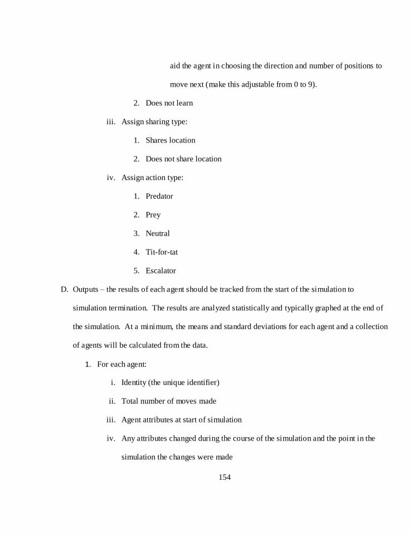
154
aid the agent in choosing the direction and number of positions to
move next (make this adjustable from 0 to 9).
2. Does not learn
iii. Assign sharing type:
1. Shares location
2. Does not share location
iv. Assign action type:
1. Predator
2. Prey
3. Neutral
4. Tit-for-tat
5. Escalator
D. Outputs – the results of each agent should be tracked from the start of the simulation to
simulation termination. The results are analyzed statistically and typically graphed at the end of
the simulation. At a minimum, the means and standard deviations for each agent and a collection
of agents will be calculated from the data.
1. For each agent:
i. Identity (the unique identifier)
ii. Total number of moves made
iii. Agent attributes at start of simulation
iv. Any attributes changed during the course of the simulation and the point in the
simulation the changes were made
155
v. Wealth of the agent at each simulation cycle – simulation cycle is chosen over
move due to allowing a variable number of simulation cycles before an agent
moves (or the equivalent terms should be used if ‗tick‘ or ‗cycle‘ is the unit of
control in the simulation. If this is changed to a variable number of moves per
simulation cycle, then agent data should be tracked per move).
2. For the landscape:
i. Distribution curve used to populate the landscape
ii. Total number of agents at start – by type
iii. Resources at each location on the landscape
Rulesets mapped to Hypotheses: The following combinations of rules will be used to evaluate
hypotheses using the simulation to generate data:
For instance, H1a (see list of hypotheses at the end of the specification) is based on rate
of movement for both the focal agent, and the responding agent – no environmental
conditions are changed (environment is neutral), and firm survival is the outcome of interest.
Therefore, the rules/agent behaviors that are used to generate data for Hypothesis 1a are
noted with H1a in the corresponding box in the table.
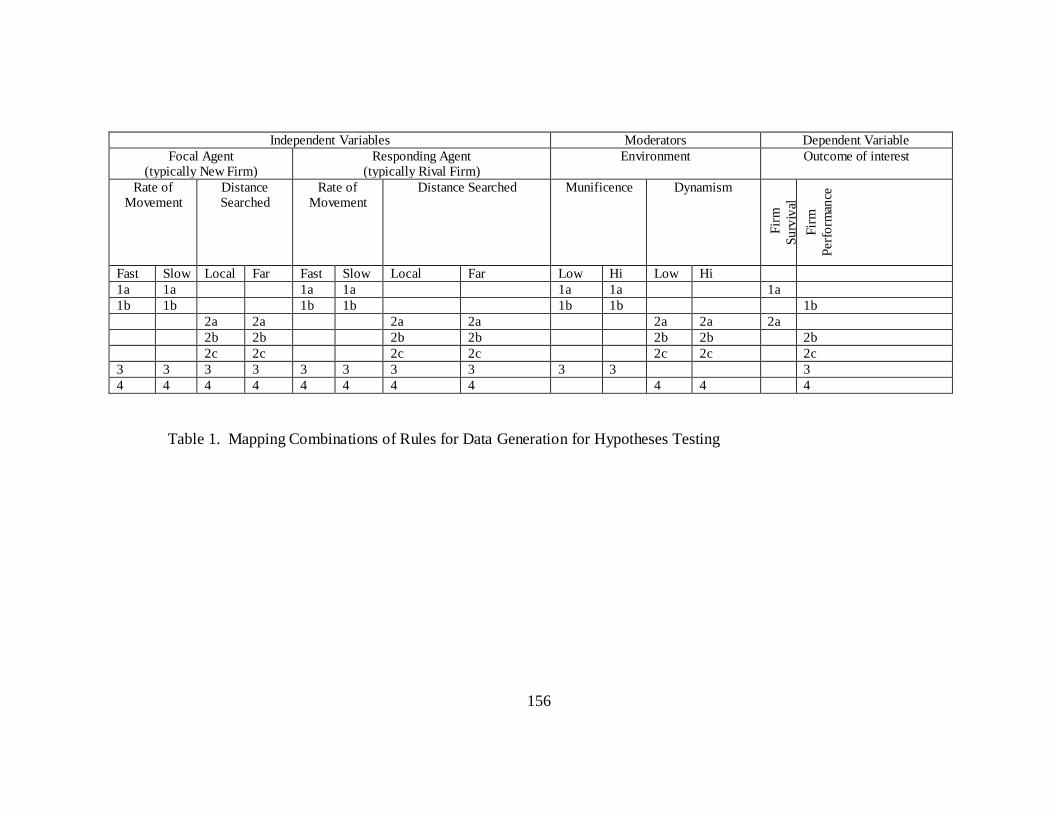
156
Independent Variables Moderators Dependent Variable
Focal Agent (typically New Firm)
Responding Agent (typically Rival Firm)
Environment Outcome of interest
Rate of Movement
Distance Searched
Rate of Movement
Distance Searched Munificence Dynamism
Fir
m
Su
rviv
al
Fir
m
Perf
orm
ance
Fast Slow Local Far Fast Slow Local Far Low Hi Low Hi
1a 1a 1a 1a 1a 1a 1a
1b 1b 1b 1b 1b 1b 1b
2a 2a 2a 2a 2a 2a 2a
2b 2b 2b 2b 2b 2b 2b
2c 2c 2c 2c 2c 2c 2c
3 3 3 3 3 3 3 3 3 3 3
4 4 4 4 4 4 4 4 4 4 4
Table 1. Mapping Combinations of Rules for Data Generation for Hypotheses Testing
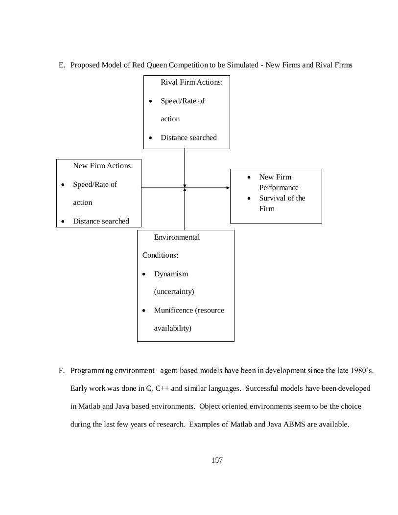
157
E. Proposed Model of Red Queen Competition to be Simulated - New Firms and Rival Firms
F. Programming environment –agent-based models have been in development since the late 1980‘s.
Early work was done in C, C++ and similar languages. Successful models have been developed
in Matlab and Java based environments. Object oriented environments seem to be the choice
during the last few years of research. Examples of Matlab and Java ABMS are available.
New Firm Actions:
Speed/Rate of
action
Distance searched
New Firm
Performance
Survival of the
Firm
Rival Firm Actions:
Speed/Rate of
action
Distance searched
Environmental
Conditions:
Dynamism
(uncertainty)
Munificence (resource
availability)

158
Further, several simulation environments are available and should be explored that are
extendable. One environment that should be considered is Repast S.

159
APPENDIX C SIMULATION PROGRAM USED TO GENERATE/COLLECT
DATA
160
NetLogo 4.1.1 was used to create the simulation model. Two types of agents were created, Red
Queen Firms and Rival Firms. Two specific actions were modeled, Moves and Searches. Environments
were generated as landscape maps with variable resources on a 20 x 20 grid. Each location‘s resource
could be varied as a function of the mean and standard deviation of the overall resources al located. Four
environment landscape maps were developed: single-peak, two-peak, multi-peak, and random. The
multi-peak was used as the primary landscape for hypothesis testing. Agents were assigned one of
several strategies for each simulation run: random direction, random direction with opportunistic
decision, pure opportunistic decision, and random direction with escalation/de-escalation. All
hypotheses were evaluated with one Red Queen Firm and one Rival Firm per simulation run.
Data collection was facilitated using the Behavior Space option in NetLogo. All input parameters
are defined for a batch of simulation runs. Output data are generated for each cycle, or tick, of the
simulation. The output can be configured as a comma separated file or an output table. 50,000
simulations were run for data collection for each hypothesis with each simulation allowed to run for 500
cycles. This generated approximately eight gigabytes of data.
The complete NetLogo code is shown below.
;; Red Queen Model - Bob Porter Version adaptive model 10 13 2010 Version 11
;; Full Copyright Robert L. Porter – all rights reserved – do not use without permission of the author
;; Version 10 includes the following features:
;; firm action controls - moves, distance, cost per move
;; munificence controls - replenishment y/n, mean of the resources distributed
;; dynamism controls - variance of resources distributed, type of resource distribution curve
;; adaptive behavior for escalation and de-escalation
;; firm search that includes opportunistic behavior = looking at options and choosing to move or not
move
;; turtles-own [new-wealth rival-wealth]
globals [
rival-move-base ; global variable used to pass rival base move count to new firm

161
rival-search-base ; global variable used to pass rival base search to new firm
new-move-base
new-search-base
how-far ;; used to determine how far a firm looks ahead when deciding to move or not in
opportunistic strategies
average-patch-resources ;; can be used when dynamic resource charges are selected - this is total
resources in the environment divided by the number of patches
cost-to-move
cost-to-look
this-new-search-distance
]
turtles-own
[
;; move tracking variables
rival-move-counter-base ;; used to pass the average of rival firm moves for new firms to check if
they need to escalate
new-move-counter-base ;; used to pass the average of new firm moves for rival firms to check if
they need to escalate
rival-move-counter ;; used to track how many moves per tick a rival firm is supposed to move
new-move-counter ;; used to track how many moves per tick a new firm is supposed to move
rival-move-counter-this-series ; used to track the moves of rival firms for the current tick series
during while loops to count down
new-move-counter-this-series ; used to track the moves of new firms for the current tick series
durring while loops to count down
avg-rival-move ; used to keep track of the rival population's average moves
avg-new-move ; used to keep track of the rival population's average moves
rival-move-display-counter ;; count of rival firm moves for the user display
new-move-display-counter ;; count of new frim moves for the user display
rival-no-move-counter ;; counts the times a rival firm can move but chooses not to
new-no-move-counter ;; counts the times a new firm can move but chooses not to
rival-no-move-display-counter ;; count of rival firm no-moves for the user display
new-no-move-display-counter ;; count of new firm no-moves for the user display
;; search tracking variables
rival-search-distance-counter

162
new-search-distance-counter
rival-search-distance-counter-this-series ; used to track the search-distance of rival firms for the
current tick series
new-search-distance-counter-this-series ; used to track the search-distance of new firms for the
current tick series
rival-search-distance-display-counter
new-search-distance-display-counter
;; escalation has been triggered
rival-move-escalated ; indicates rival firm moves have been escalated
new-move-escalated ; indicates new firm moves have been escalated
;; running total (cumulative) of firm wealth
rival-firm-cum-wealth ; the running total, or cumulative wealth earned by firms for the simulation
run
new-firm-cum-wealth ; the running total, or cumulative wealth earned by firms for the simulation
run
]
patches-own
[
resource-here ; the current amount of resource on this patch
max-resource-here ; the maximum amount of resource this patch can hold
]
breed [new-firms new-firm]
breed [rival-firms rival-firm]
new-firms-own [
new-firm-wealth ; a performance variable for new firms - the current value of new firm wealth
; new-firm-cum-wealth ; the running total, or cumulative wealth earned by firms for the simulation
run
]
rival-firms-own [
rival-firm-wealth ; a performance variable for rival firms - the current value of new firm wealth
; rival-firm-cum-wealth ; the running total, or cumulative wealth earned by firms for the simulation
run
]
163
to setup
clear-all
setup-patches
setup-firms
end
to setup-patches
if Resource-Landscape = "Random"
[
ask patches [
; to setup initial amount of resource on a patch
if Dynamism-mode = "Exponential-resource-curve"
[set resource-here random-exponential resource-mean] ;; set initial resources randomly between 0
to max-resource-value
if Dynamism-mode = "Normal-resource-curve"
[set resource-here random-normal resource-mean resource-standard-deviation] ;; set initial
resources randomly between 0 to max-resource-value
if cap-location-resource = true ; to set the initial amount of resource as the maximum amount of
resources ever on this patch
[ set max-resource-here resource-here]
if cap-location-resource = false ; if no cap on resources, then just use the input from the user to set
the max
[ set max-resource-here max-resource-value]
set average-patch-resources mean [resource-here] of patches ;; this is used when dynamic cost per
move & look is selected by the user
set pcolor (60 - ((resource-here / max-resource-value) * 7)) ; set up the initial patch color to reflect
the resources on the patch - light green/white = low, dark green = high
]
]
if Resource-Landscape = "No Peak"
[
file-open "no-peak.txt"
foreach sort patches
[
ask ?
[
set resource-here file-read * (resource-mean / 10 )
164
if cap-location-resource = true ; to set the initial amount of resource as the maximum amount of
resources ever on this patch
[ set max-resource-here resource-here]
if cap-location-resource = false ; if no cap on resources, then just use the input from the user to
set the max
[ set max-resource-here max-resource-value]
set pcolor (60 - ((resource-here / max-resource-value) * 7)) ; set up the initial patch color to
reflect the resources on the patch - light green/white = low, dark green = hig
]
]
set average-patch-resources mean [resource-here] of patches
file-close
]
if Resource-Landscape = "Simple One Peak"
[
file-open "simple-one-peak.txt"
foreach sort patches
[
ask ?
[
set resource-here file-read * (resource-mean / 10 )
if cap-location-resource = true ; to set the initial amount of resource as the maximum amount of
resources ever on this patch
[ set max-resource-here resource-here]
if cap-location-resource = false ; if no cap on resources, then just use the input from the user to
set the max
[ set max-resource-here max-resource-value]
set pcolor (60 - ((resource-here / max-resource-value) * 7)) ; set up the initial patch color to
reflect the resources on the patch - light green/white = low, dark green = hig
]
]
set average-patch-resources mean [resource-here] of patches
file-close
]
if Resource-Landscape = "Simple One Peak V2"
[
file-open "simple-one-peak v2.txt"
foreach sort patches
[
ask ?
[
set resource-here file-read * (resource-mean / 10 )

165
if cap-location-resource = true ; to set the initial amount of resource as the maximum amount of
resources ever on this patch
[ set max-resource-here resource-here]
if cap-location-resource = false ; if no cap on resources, then just use the input from the user to
set the max
[ set max-resource-here max-resource-value]
set pcolor (60 - ((resource-here / max-resource-value) * 7)) ; set up the initial patch color to
reflect the resources on the patch - light green/white = low, dark green = hig
]
]
set average-patch-resources mean [resource-here] of patches
file-close
]
if Resource-Landscape = "Simple One Peak V3"
[
file-open "simple-one-peak v3.txt"
foreach sort patches
[
ask ?
[
set resource-here file-read * (resource-mean / 10 )
if cap-location-resource = true ; to set the initial amount of resource as the maximum amount of
resources ever on this patch
[ set max-resource-here resource-here]
if cap-location-resource = false ; if no cap on resources, then just use the input from the user to
set the max
[ set max-resource-here max-resource-value]
set pcolor (60 - ((resource-here / max-resource-value) * 7)) ; set up the initial patch color to
reflect the resources on the patch - light green/white = low, dark green = hig
]
]
set average-patch-resources mean [resource-here] of patches
file-close
]
if Resource-Landscape = "Two Peaks"
[
file-open "Two-peak.txt"
foreach sort patches
[
ask ?
[
set resource-here file-read * (resource-mean / 10 )
166
if cap-location-resource = true ; to set the initial amount of resource as the maximum amount of
resources ever on this patch
[ set max-resource-here resource-here]
if cap-location-resource = false ; if no cap on resources, then just use the input from the user to
set the max
[ set max-resource-here max-resource-value]
set pcolor (60 - ((resource-here / max-resource-value) * 7)) ; set up the initial patch color to
reflect the resources on the patch - light green/white = low, dark green = hig
]
]
set average-patch-resources mean [resource-here] of patches
file-close
]
if Resource-Landscape = "Rugged Multi-Peak"
[
file-open "multi-peak.txt"
foreach sort patches
[
ask ?
[
set resource-here file-read * (resource-mean / 10 )
if cap-location-resource = true ; to set the initial amount of resource as the maximum amount of
resources ever on this patch
[ set max-resource-here resource-here]
if cap-location-resource = false ; if no cap on resources, then just use the input from the user to
set the max
[ set max-resource-here max-resource-value]
set pcolor (60 - ((resource-here / max-resource-value) * 7)) ; set up the initial patch color to
reflect the resources on the patch - light green/white = low, dark green = hig
]
]
set average-patch-resources mean [resource-here] of patches
file-close
]
end
to setup-firms ;; both new and rival firms
set-default-shape new-firms "new-firms" ;; each firm has a distinct shape - new is a cap F
set-default-shape rival-firms "rival-firm" ;; each firm has a distinct shape - rival is a cap R
;; set no-move-counter 0
create-new-firms (percent-new-firms * number-of-initial-firms) ;; determine number of firms to
be new from input from user
[
setxy random-pxcor random-pycor ; new firm setup
167
set breed new-firms
set color red
set size 1.5
set heading random 360
while [any? other new-firms-here or any? other rival-firms-here] [fd 1] ; move to a patch with no
new firm on it
set new-firm-wealth initial-wealth ;;
]
create-rival-firms ((1.0 - percent-new-firms) * number-of-initial-firms) ;; determine number of
firms to be rival
[
setxy random-pxcor random-pycor ; rival firm setup
set breed rival-firms
set color cyan
set size 1.5
set heading random 360
while [any? other rival-firms-here or any? other new-firms-here] [fd 1]
set rival-firm-wealth initial-wealth ;; set initial wealth level of firms using input panel number
]
end
to go
if stop-when-no-firms = true ; see if we should stop if all firms are gone
[
if not any? rival-firms and not any? new-firms ; check both firm types
[
stop ; stop if no firms alive
]
]
ask turtles ; must be some firms, so do the firm actions
[
choose-strategy ;; based on user choice from chooser input
; choose-move ;; move all firms on the landscape based on move routines
; choose-search ;; move all firms on the landscape based on search routines
]
ask patches ; must be some firms, so do the environment actions
[
recolor-resource ;; color the landscape
replenish-resource ;; replenish the landscape = munificence
]
tick
end
;;;;;;;;;;;;; Choose Strategy ;;;;;;;;;;;;;;;;
168
to choose-strategy ;; first determine which type of firm is selecting a strategy, new or rival firms
set new-move-escalated 0
ifelse breed = rival-firms ;; check breed - rival or new firm
[ rival-strategies ]
[ new-strategies ]
end
to rival-strategies ;; see what the user has selected for the rival strategy and go there
;;;;----- Move strategies ------;;;;
if rival-firm-strategy-type = "Random Direction Moves"
[ rival-move-strategy-random-direction-moves ]
;if rival-firm-strategy-type = "Random Move w Escalation"
; [ rival-move-strategy-random-Esc ]
if rival-firm-strategy-type = "Random Direction & Number Moves" ;; this is escalation and de-
escalation
[ rival-move-strategy-random-direction-and-number-moves ]
;if rival-firm-strategy-type = "Random Move w Trig Esc"
; [rival-move-strategy-random-Trig-Esc]
if rival-firm-strategy-type = "Random Opportunistic Move"
[ rival-move-strategy-random-Opportunistic ]
if rival-firm-strategy-type = "Random Opp Move w Esc/De-Esc due to no moves"
[ rival-move-strategy-random-Opportunistic-Esc/De-Esc ]
if rival-firm-strategy-type = "Random Opp Move w trig Esc"
[ rival-move-strategy-random-Opportunistic-Trig-Esc ]
if rival-firm-strategy-type = "Pure Opportunistic Move"
[ rival-move-strategy-pure-Opportunistic ]
;if rival-firm-strategy-type = "Pure Opp Move w Trip Esc/De-Esc"
; [ rival-move-strategy-pure-Opportunistic-Trig-Esc-DeEsc]
;;;;----- Search strategies ------;;;;
if rival-firm-strategy-type = "Random Search"
[ rival-search-strategy-random ]
stop
end
to new-strategies ;; see what the user has selected for the new firm strategy and go there
;;;;----- Move strategies ------;;;;
if new-firm-strategy-type = "Random Direction Moves"
[ new-move-strategy-random-direction-moves ]
; if new-firm-strategy-type = "Random Move w Escalation"
; [new-move-strategy-random-Esc]
if new-firm-strategy-type = "Random Direction & Number Moves" ;; this is escalation and de-
escalation
[ new-move-strategy-random-direction-and-number-moves ]
169
if new-firm-strategy-type = "Random Direction & Random Distance Moved"
[ new-move-strategy-random-direction-and-random-distance ]
;if new-firm-strategy-type = "Random Move w Trig Esc"
; [ ]
if new-firm-strategy-type = "Random Opportunistic Move"
[ new-move-strategy-random-Opportunistic ]
if new-firm-strategy-type = "Random Opp Move w Esc/De-Esc due to no moves"
[ new-move-strategy-random-Opportunistic-Esc/De-Esc ]
if new-firm-strategy-type = "Random Opp Move w trig Esc"
[ new-move-strategy-random-Opportunistic-Trig-Esc ]
;if new-firm-strategy-type = "Random Opp Move w Trip Esc/De-Esc"
; [ new-move-strategy-Opportunistic-Trig-Esc-DeEsc]
if new-firm-strategy-type = "Pure Opportunistic Move"
[ new-move-strategy-pure-Opportunistic ]
if new-firm-strategy-type = "Pure Opp Move w Trip Esc/De-Esc"
[ new-move-strategy-pure-Opportunistic-Trig-Esc-DeEsc]
;;;;----- Search strategies ------;;;;
if new-firm-strategy-type ="Random Balanced Search"
[ new-search-strategy-random-balanced ]
if new-firm-strategy-type ="Opp Balanced Search"
[ new-search-strategy-opportunistic-balanced ]
stop
end
to choose-cost-of-actions
if Fixed-or-dynamic-resources-used = "Fixed based on user input"
[ set cost-to-move units-of-resource-used-per-action
set cost-to-look units-of-resource-used-per-look
]
if Fixed-or-dynamic-resources-used = "Dyanmic based on Environment"
[ set cost-to-move average-patch-resources ;; use the average of the resources places on the patches
set cost-to-look (average-patch-resources * .33 ) ;; use 1/3 of the average of the resources
]
end
;;;;; Rival move firm strategies ;;;; These are all 'move' based strategies (not search distance unless
the search distance is > 1) ;;;;;
to rival-move-strategy-random-direction-moves ;; basic strategy - the firm moves in random
directions a fixed number of moves to find resources
choose-cost-of-actions
set rival-move-counter rival-moves-per-tick ;; initialize the rival move counter to what the user
requests

170
set rival-search-distance-counter rival-search-distance-per-tick ;; initialize the rival search counter
to what the user requests
while [ rival-move-counter > 0 ] ;; do this next command set while more than one move if move is
set to more than one by user
[
set rival-move-display-counter rival-move-display-counter + 1 ;; the display counter is used to
give feedback on the control panel
set rival-search-distance-display-counter rival-search-distance-display-counter + rival-search-
distance-per-tick ;; the display counter is used to give feedback on the control panel
set rival-move-counter rival-move-counter - 1.0 ;; down count the move counter
set heading random 360 ;; pick a random direction
fd rival-search-distance-per-tick;; move the search distance specified from the input panel- so this
can be used for search routines as well
set rival-firm-wealth ( rival-firm-wealth + resource-here - cost-to-move - cost-to-look * rival-
search-distance-per-tick );; increment wealth but charge for the move
set rival-firm-cum-wealth rival-firm-cum-wealth + rival-firm-wealth
set resource-here 0 ;; set resource on this patch to zero
rival-firm-data-output ;; standard output procedure for plots and user monitors on user interface
and for behavior space data collection
]
if rival-firm-wealth < 0 [ die ] ;; kill the firm if wealth is too low
end
to rival-move-strategy-random-Esc
choose-cost-of-actions
; set rival-move-counter-this-series random max-rival-move ; initialize the number of moves for the
rival agents as a random number from 0 to max rival move
set rival-move-counter rival-move-counter-this-series ; initialize the counter used in the commands
below
set rival-move-base rival-move-counter-this-series ; initialize the global variable to be passed to
new firms
set rival-search-distance-counter rival-search-distance-per-tick ;; initialize the rival search counter
to what the user requests
;; not developed yet
end
to rival-move-strategy-random-direction-and-number-moves ;; basic strategy moving in random
direction with random escalation and de-escalation
choose-cost-of-actions
set rival-move-counter-this-series random max-rival-move ; initialize the number of moves for the
rival agents as a random number from 0 to max rival move
171
set rival-move-counter rival-move-counter-this-series ; initialize the counter used in the commands
below
set rival-move-base rival-move-counter-this-series ; initialize the global variable to be passed to
new firms
set rival-search-distance-counter rival-search-distance-per-tick ;; initialize the rival search counter
to what the user requests
while [ rival-move-counter > 0 ] ;; more than one move if move is set to more than one by user
[
set rival-move-display-counter rival-move-display-counter + 1 ;; increment the move counter on
the user panel
set rival-move-counter rival-move-counter - 1.0 ; decrement the move-counter
set heading random 360 ; move in a random direction
fd rival-search-distance-per-tick;; move the search distance specified from the input panel
set rival-search-distance-display-counter rival-search-distance-display-counter + rival-search-
distance-per-tick ;; the display counter is used to give feedback on the control panel
set rival-firm-wealth ( rival-firm-wealth + resource-here - cost-to-move - cost-to-look ) ;;
increment the agent's wealth by the amount of resource on the
;; and decrease it by the amount it costs to move
set rival-firm-cum-wealth rival-firm-cum-wealth + rival-firm-wealth
set resource-here 0 ;; set resource on this patch to zero
rival-firm-data-output ;; standard output procedure for plots and user monitors on user interface
and for behavior space data collection
]
if rival-firm-wealth < 0 [ die ]
end
to rival-move-strategy-random-Trig-Esc
choose-cost-of-actions
set rival-search-distance-counter rival-search-distance-per-tick ;; initialize the rival search counter to
what the user requests
end
to rival-move-strategy-random-Opportunistic ;; one move checking opportunistic strategy - check to
see if the patch you would move to has higher resources
choose-cost-of-actions
set rival-move-counter rival-moves-per-tick ;; initialize the rival move counter
set rival-search-distance-counter rival-search-distance-per-tick ;; initialize the rival search counter
to what the user requests
while [ rival-move-counter > 0 ] ;; do this next command set while more than one move if move is
set to more than one by user
[
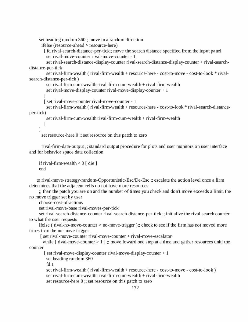
172
set heading random 360 ; move in a random direction
ifelse (resource-ahead > resource-here)
[ fd rival-search-distance-per-tick;; move the search distance specified from the input panel
set rival-move-counter rival-move-counter - 1
set rival-search-distance-display-counter rival-search-distance-display-counter + rival-search-
distance-per-tick
set rival-firm-wealth ( rival-firm-wealth + resource-here - cost-to-move - cost-to-look * rival-
search-distance-per-tick )
set rival-firm-cum-wealth rival-firm-cum-wealth + rival-firm-wealth
set rival-move-display-counter rival-move-display-counter + 1
]
[ set rival-move-counter rival-move-counter - 1
set rival-firm-wealth ( rival-firm-wealth + resource-here - cost-to-look * rival-search-distance-
per-tick)
set rival-firm-cum-wealth rival-firm-cum-wealth + rival-firm-wealth
]
]
set resource-here 0 ;; set resource on this patch to zero
rival-firm-data-output ;; standard output procedure for plots and user monitors on user interface
and for behavior space data collection
if rival-firm-wealth < 0 [ die ]
end
to rival-move-strategy-random-Opportunistic-Esc/De-Esc ;; escalate the action level once a firm
determines that the adjacent cells do not have more resources
;; than the patch you are on and the number of times you check and don't move exceeds a limit, the
no move trigger set by user
choose-cost-of-actions
set rival-move-base rival-moves-per-tick
set rival-search-distance-counter rival-search-distance-per-tick ;; initialize the rival search counter
to what the user requests
ifelse ( rival-no-move-counter > no-move-trigger );; check to see if the firm has not moved more
times than the no-move trigger
[ set rival-move-counter rival-move-counter + rival-move-escalator
while [ rival-move-counter > 1 ] ;; move foward one step at a time and gather resources unitl the
counter
[ set rival-move-display-counter rival-move-display-counter + 1
set heading random 360
fd 1
set rival-firm-wealth ( rival-firm-wealth + resource-here - cost-to-move - cost-to-look )
set rival-firm-cum-wealth rival-firm-cum-wealth + rival-firm-wealth
set resource-here 0 ;; set resource on this patch to zero
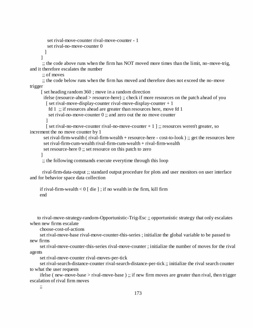
173
set rival-move-counter rival-move-counter - 1
set rival-no-move-counter 0
]
]
;; the code above runs when the firm has NOT moved more times than the limit, no-move-trig,
and it therefore escalates the number
;; of moves
;; the code below runs when the firm has moved and therefore does not exceed the no-move
trigger
[ set heading random 360 ; move in a random direction
ifelse (resource-ahead > resource-here) ;; check if more resources on the patch ahead of you
[ set rival-move-display-counter rival-move-display-counter + 1
fd 1 ;; if resources ahead are greater than resources here, move fd 1
set rival-no-move-counter 0 ;; and zero out the no move counter
]
[ set rival-no-move-counter rival-no-move-counter + 1 ] ;; resources weren't greater, so
increment the no move counter by 1
set rival-firm-wealth ( rival-firm-wealth + resource-here - cost-to-look ) ;; get the resources here
set rival-firm-cum-wealth rival-firm-cum-wealth + rival-firm-wealth
set resource-here 0 ;; set resource on this patch to zero
]
;; the following commands execute everytime through this loop
rival-firm-data-output ;; standard output procedure for plots and user monitors on user interface
and for behavior space data collection
if rival-firm-wealth < 0 [ die ] ; if no wealth in the firm, kill firm
end
to rival-move-strategy-random-Opportunistic-Trig-Esc ;; opportunistic strategy that only escalates
when new firms escalate
choose-cost-of-actions
set rival-move-base rival-move-counter-this-series ; initialize the global variable to be passed to
new firms
set rival-move-counter-this-series rival-move-counter ; initialize the number of moves for the rival
agents
set rival-move-counter rival-moves-per-tick
set rival-search-distance-counter rival-search-distance-per-tick ;; initialize the rival search counter
to what the user requests
ifelse ( new-move-base > rival-move-base ) ;; if new firm moves are greater than rival, then trigger
escalation of rival firm moves
;;
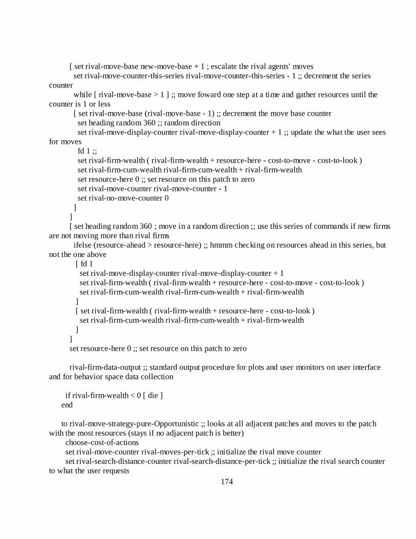
174
[ set rival-move-base new-move-base + 1 ; escalate the rival agents' moves
set rival-move-counter-this-series rival-move-counter-this-series - 1 ;; decrement the series
counter
while [ rival-move-base > 1 ] ;; move foward one step at a time and gather resources until the
counter is 1 or less
[ set rival-move-base (rival-move-base - 1) ;; decrement the move base counter
set heading random 360 ;; random direction
set rival-move-display-counter rival-move-display-counter + 1 ;; update the what the user sees
for moves
fd 1 ;;
set rival-firm-wealth ( rival-firm-wealth + resource-here - cost-to-move - cost-to-look )
set rival-firm-cum-wealth rival-firm-cum-wealth + rival-firm-wealth
set resource-here 0 ;; set resource on this patch to zero
set rival-move-counter rival-move-counter - 1
set rival-no-move-counter 0
]
]
[ set heading random 360 ; move in a random direction ;; use this series of commands if new firms
are not moving more than rival firms
ifelse (resource-ahead > resource-here) ;; hmmm checking on resources ahead in this series, but
not the one above
[ fd 1
set rival-move-display-counter rival-move-display-counter + 1
set rival-firm-wealth ( rival-firm-wealth + resource-here - cost-to-move - cost-to-look )
set rival-firm-cum-wealth rival-firm-cum-wealth + rival-firm-wealth
]
[ set rival-firm-wealth ( rival-firm-wealth + resource-here - cost-to-look )
set rival-firm-cum-wealth rival-firm-cum-wealth + rival-firm-wealth
]
]
set resource-here 0 ;; set resource on this patch to zero
rival-firm-data-output ;; standard output procedure for plots and user monitors on user interface
and for behavior space data collection
if rival-firm-wealth < 0 [ die ]
end
to rival-move-strategy-pure-Opportunistic ;; looks at all adjacent patches and moves to the patch
with the most resources (stays if no adjacent patch is better)
choose-cost-of-actions
set rival-move-counter rival-moves-per-tick ;; initialize the rival move counter
set rival-search-distance-counter rival-search-distance-per-tick ;; initialize the rival search counter
to what the user requests
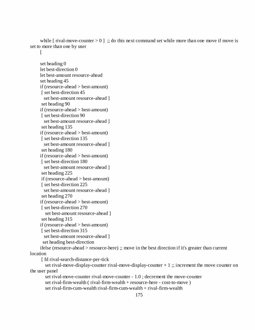
175
while [ rival-move-counter > 0 ] ;; do this next command set while more than one move if move is
set to more than one by user
[
set heading 0
let best-direction 0
let best-amount resource-ahead
set heading 45
if (resource-ahead > best-amount)
[ set best-direction 45
set best-amount resource-ahead ]
set heading 90
if (resource-ahead > best-amount)
[ set best-direction 90
set best-amount resource-ahead ]
set heading 135
if (resource-ahead > best-amount)
[ set best-direction 135
set best-amount resource-ahead ]
set heading 180
if (resource-ahead > best-amount)
[ set best-direction 180
set best-amount resource-ahead ]
set heading 225
if (resource-ahead > best-amount)
[ set best-direction 225
set best-amount resource-ahead ]
set heading 270
if (resource-ahead > best-amount)
[ set best-direction 270
set best-amount resource-ahead ]
set heading 315
if (resource-ahead > best-amount)
[ set best-direction 315
set best-amount resource-ahead ]
set heading best-direction
ifelse (resource-ahead > resource-here) ;; move in the best direction if it's greater than current
location
[ fd rival-search-distance-per-tick
set rival-move-display-counter rival-move-display-counter + 1 ;; increment the move counter on
the user panel
set rival-move-counter rival-move-counter - 1.0 ; decrement the move-counter
set rival-firm-wealth ( rival-firm-wealth + resource-here - cost-to-move )
set rival-firm-cum-wealth rival-firm-cum-wealth + rival-firm-wealth
176
]
[ set rival-move-counter rival-move-counter - 1.0 ; decrement the move-counter
set rival-firm-wealth ( rival-firm-wealth + resource-here - ( cost-to-look * rival-search-distance-
per-tick ))
set rival-firm-cum-wealth rival-firm-cum-wealth + rival-firm-wealth
]
]
set resource-here 0 ;; set resource on this patch to zero
rival-firm-data-output ;; standard output procedure for plots and user monitors on user interface
and for behavior space data collection
if rival-firm-wealth < 0 [ die ]
end
to rival-move-strategy-Opportunistic-Trig-Esc-DeEsc
choose-cost-of-actions
set rival-search-distance-counter rival-search-distance-per-tick ;; initialize the rival search counter
to what the user requests
end
;;;;; Rival firm Search strategies ;;;; These are all 'search' based strategies (not just move distance)
;;;;;
to rival-search-strategy-random ;; basic search strategy - the firm moves in random directions a
fixed number of moves
choose-cost-of-actions
set rival-search-distance-counter rival-search-distance-per-tick ;; initialize the new search counter
to what the user requests
set heading random 360
fd rival-search-distance-per-tick;; move the search distance specified from the input panel
set rival-search-distance-display-counter rival-search-distance-display-counter + rival-search-
distance-per-tick
set rival-firm-wealth ( rival-firm-wealth + resource-here - cost-to-move - ( cost-to-look * rival-
search-distance-per-tick ) )
set new-firm-cum-wealth new-firm-cum-wealth + new-firm-wealth
set resource-here 0 ;; set resource on this patch to zero
rival-firm-data-output ;; standard output procedure for plots and user monitors on user interface
and for behavior space data collection
if rival-firm-wealth < 0 [ die ]
end
177
;;;;; Key procedure used by firms to look ahead to check resources compared to the current location
to-report resource-ahead ;; firm procedure to determine what resources on on the patch ahead
ifelse breed = rival-firms ;; check breed - rival or new firm
[ set how-far rival-search-distance-per-tick + .5 ]
[ set how-far new-search-distance-per-tick + .5 ]
let total 0 ;; set total as a temporary value to zero
; let how-far 1.5 ;; this determines how far ahead to look - use a number greater than one to insure
you are looking one patch ahead
set total total + [resource-here] of patch-ahead how-far ;; total is incremented to value of resources
on the next patch ahead
report total ;; new total value is reported as resource-ahead value
end
;;;;; New firm strategies ;;;; These are all 'move' based strategies (not search distance) ;;;;;
to new-move-strategy-random-direction-moves ;; basic strategy - the firm moves in random
directions a fixed number of moves
choose-cost-of-actions
set new-move-counter new-moves-per-tick ;; more than one move if move is set to more than one
by user
set new-search-distance-counter new-search-distance-per-tick ;; initialize the new search counter to
what the user requests
while [ new-move-counter > 0 ]
[
set new-move-counter new-move-counter - 1.0
set heading random 360
set new-move-display-counter new-move-display-counter + 1
set new-search-distance-display-counter new-search-distance-display-counter + new-search-
distance-per-tick ;; the display counter is used to give feedback on the control panel
fd new-search-distance-per-tick ;; move the distance set by user, so this works for search and
move actions
set new-firm-wealth ( new-firm-wealth + resource-here - cost-to-move - cost-to-look * new-
search-distance-per-tick )
set new-firm-cum-wealth new-firm-cum-wealth + new-firm-wealth
set resource-here 0 ;; set resource on this patch to zero
new-firm-data-output ;; standard output procedure for plots and user monitors on user interface
and for behavior space data collection
]
if new-firm-wealth < 0 [ die ]
end

178
to new-move-strategy-random-direction-and-number-moves ;; basic strategy moving in random
direction with random escalation and de-escalation
choose-cost-of-actions
set new-move-counter-this-series random max-new-move ; initialize the number of moves for the
new agents as a random number from 0 to new rival move
set new-move-counter new-move-counter-this-series ; initialize the counter used in the commands
below
set new-move-base new-move-counter-this-series ; initialize the global variable to be passed to new
firms
set new-search-distance-counter new-search-distance-per-tick ;; initialize the rival search counter to
what the user requests
while [ new-move-counter > 0 ]
[
set new-move-counter new-move-counter - 1.0
set heading random 360
set new-move-display-counter new-move-display-counter + 1
fd new-search-distance-per-tick ;; move the distance set by user, so this works for search and move
actions
set new-search-distance-display-counter new-search-distance-display-counter + new-search-
distance-per-tick ;; the display counter is used to give feedback on the control panel
set new-firm-wealth ( new-firm-wealth + resource-here - cost-to-move - cost-to-look )
set new-firm-cum-wealth new-firm-cum-wealth + new-firm-wealth
set resource-here 0 ;; set resource on this patch to zero
new-firm-data-output ;; standard output procedure for plots and user monitors on user interface and
for behavior space data collection
]
if new-firm-wealth < 0 [ die ]
end
to new-move-strategy-random-direction-and-random-distance ;; basic strategy moving in random
direction with random escalation and de-escalation
choose-cost-of-actions
set new-search-distance-counter-this-series random max-new-search ; initialize the distance
searched for the new agents as a random number from 0 to max new distance search
set new-search-distance-counter new-search-distance-counter-this-series ; initialize the counter
used in the commands below
set new-search-base new-search-distance-counter-this-series ; initialize the global variable to be
passed to rival firms for escalation procedures
while [ new-search-distance-counter > 0 ]
179
[
set heading random 360
fd new-search-distance-counter ;; jump the distance set by random selection made above
set new-search-distance-display-counter new-search-distance-display-counter + new-search-
distance-counter ;; the display counter is used to give feedback on the control panel
set new-firm-wealth ( new-firm-wealth + resource-here - cost-to-move - ( cost-to-look * new-
search-distance-counter ))
set new-firm-cum-wealth new-firm-cum-wealth + new-firm-wealth
set resource-here 0 ;; set resource on this patch to zero
set new-search-distance-counter new-search-distance-counter - 1.0 ;; down count the random
selection made above by 1
new-firm-data-output ;; standard output procedure for plots and user monitors on user interface and
for behavior space data collection
]
if new-firm-wealth < 0 [ die ]
set new-search-distance-counter-this-series new-search-distance-per-tick ;; reset the series counter
in case it's used somewhere else
end
to new-move-strategy-random-Opportunistic ;; opportunistic strategy - find the patch with the most
resources
choose-cost-of-actions
set new-move-counter new-moves-per-tick ;; more than one move if move is set to more than one
by user
set new-search-distance-display-counter new-search-distance-per-tick ;; initialize the new search
counter to what the user requests
while [ new-move-counter > 0 ]
[
set heading random 360 ; move in a random direction
ifelse (resource-ahead > resource-here)
[ fd new-search-distance-per-tick ;; move the distance set by user, so this works for search and
move actions
set new-move-counter new-move-counter - 1
set new-search-distance-display-counter new-search-distance-display-counter + new-search-
distance-per-tick
set new-firm-wealth ( new-firm-wealth + resource-here - cost-to-move - cost-to-look * new-
search-distance-per-tick )
set new-firm-cum-wealth new-firm-cum-wealth + new-firm-wealth
set new-move-display-counter new-move-display-counter + 1
]
[ set new-move-counter new-move-counter - 1
180
set new-firm-wealth ( new-firm-wealth + resource-here - cost-to-look * new-search-distance-
per-tick)
set new-firm-cum-wealth new-firm-cum-wealth + new-firm-wealth
]
]
set resource-here 0 ;; set resource on this patch to zero
new-firm-data-output ;; standard output procedure for plots and user monitors on user interface and
for behavior space data collection
if new-firm-wealth < 0 [ die ]
end
to new-move-strategy-random-Opportunistic-Esc/De-Esc ;; escalate the action level once a firm
determines that the adjacent cells do not have more resources
;; than the patch you are on and you have 'not moved' a sufficient number of times to exceed the no-
move trigger
choose-cost-of-actions
set new-move-base new-moves-per-tick
set new-search-distance-counter new-search-distance-per-tick ;; initialize the new search counter to
what the user requests
ifelse ( new-no-move-counter > no-move-trigger );; check to see if the firm has not moved more
times than the no-move limit trigger
[ set new-move-escalated 1 ;; indicate that an escalation has been triggered
set new-move-counter new-move-counter + new-move-escalator ;; escalate the number of moves
the new firm makes
while [ new-move-counter > 1 ] ;; move foward one step at a time and gather resources until the
counter is back to 1
[ set heading random 360
set new-move-display-counter new-move-display-counter + 1 ;; increment the display tracking
the number of moves
fd 1 ;; move forward
set new-firm-wealth ( new-firm-wealth + resource-here - cost-to-move - cost-to-look )
set new-firm-cum-wealth new-firm-cum-wealth + new-firm-wealth
set resource-here 0 ;; set resource on this patch to zero
set new-move-counter new-move-counter - 1 ;; decrement the new move counter
]
set new-no-move-counter 0
]
;; the code above runs when the firm has NOT moved more times than the limit, no-move-trig,
and it therefore escalates the number
;; of moves
181
;; the code below runs when the firm has moved and therefore does not exceed the no-move
trigger
[ set heading random 360 ; move in a random direction
ifelse (resource-ahead > resource-here) ;; check if more resources on the patch ahead of you
[ set new-move-display-counter new-move-display-counter + 1
fd 1 ;; if resources ahead are greater than resources here, move fd 1
set new-no-move-counter 0 ;; and zero out the no move counter
]
[ set new-no-move-counter new-no-move-counter + 1
] ;; adjacent resources weren't greater, so increment the no move counter by 1
set new-firm-wealth ( new-firm-wealth + resource-here - cost-to-look );; get the resources here
set new-firm-cum-wealth new-firm-cum-wealth + new-firm-wealth
set resource-here 0 ;; set resource on this patch to zero
]
;; the following commands execute everytime through this loop
new-firm-data-output ;; standard output procedure for plots and user monitors on user interface
and for behavior space data collection
if new-firm-wealth < 0 [ die ] ; if no wealth in the firm, kill firm
end
to new-move-strategy-random-Opportunistic-Trig-Esc ;; opportunistic strategy that only escalates
when rival firms escalate
choose-cost-of-actions
set new-move-counter new-moves-per-tick
set new-move-counter-this-series new-move-counter ; initialize the number of moves for the new
agents
;; set new-move-counter new-move-counter-this-series ; initialize the counter used in the
commands below
set new-move-base new-move-counter-this-series ; initialize the global variable to be passed to new
firms
set new-search-distance-counter new-search-distance-per-tick ;; initialize the new search counter to
what the user requests
ifelse ( rival-move-base > new-move-base ) ;; if rival greater, then trigger escalation of new firms
;;
[ set new-move-base new-move-base + 1 ;; this is the escalation
while [ new-move-base > 1 ] ;; move foward one step at a time and gather resources unitl the
counter
[ set new-move-base (new-move-base - 1) ;; decrement the escalation factor
set heading random 360
set new-move-display-counter new-move-display-counter + 1
fd 1
set new-firm-wealth ( new-firm-wealth + resource-here - cost-to-move - cost-to-look )
182
set new-firm-cum-wealth new-firm-cum-wealth + new-firm-wealth
set resource-here 0 ;; set resource on this patch to zero
set new-move-counter new-move-counter - 1
set new-no-move-counter 0
]
]
[ set heading random 360 ; move in a random direction
ifelse (resource-ahead > resource-here)
[ set new-move-display-counter new-move-display-counter + 1
fd 1
set new-firm-wealth ( new-firm-wealth + resource-here - cost-to-move - cost-to-look )
set new-firm-cum-wealth new-firm-cum-wealth + new-firm-wealth
]
[ set new-firm-wealth ( new-firm-wealth + resource-here - cost-to-look )
set new-firm-cum-wealth new-firm-cum-wealth + new-firm-wealth
]
]
set resource-here 0 ;; set resource on this patch to zero
new-firm-data-output ;; standard output procedure for plots and user monitors on user interface
and for behavior space data collection
if new-firm-wealth < 0 [ die ]
end
to new-move-strategy-pure-Opportunistic ;; opportunistic strategy - find the adjacent patch with the
most resources and moves there and
;; stop moving when you find the patch
;; check all adjacent patches with the following commands and determine the optimum heading
choose-cost-of-actions
set new-move-counter new-moves-per-tick ;; more than one move if move is set to more than one
by user
set new-search-distance-counter new-search-distance-per-tick ;; initialize the new search counter to
what the user requests
while [ new-move-counter > 0 ]
[
set heading 0
let best-direction 0
let best-amount resource-ahead
set heading 45
if (resource-ahead > best-amount)
[ set best-direction 45

183
set best-amount resource-ahead ]
set heading 90
if (resource-ahead > best-amount)
[ set best-direction 90
set best-amount resource-ahead ]
set heading 135
if (resource-ahead > best-amount)
[ set best-direction 135
set best-amount resource-ahead ]
set heading 180
if (resource-ahead > best-amount)
[ set best-direction 180
set best-amount resource-ahead ]
set heading 225
if (resource-ahead > best-amount)
[ set best-direction 225
set best-amount resource-ahead ]
set heading 270
if (resource-ahead > best-amount)
[ set best-direction 270
set best-amount resource-ahead ]
set heading 315
if (resource-ahead > best-amount)
[ set best-direction 315
set best-amount resource-ahead ]
set heading best-direction
;;
;; the above determines the best direction, now to move in that direction - note the heading will stay
the same if the firm is
;; already on the patch with the greatest resources relative to the adjacent patches
;;
ifelse (resource-ahead > resource-here) ;; move in the best direction if it's greater than current
location
[ fd new-search-distance-per-tick
set new-move-counter new-move-counter - 1.0
set new-move-display-counter new-move-display-counter + 1
set new-firm-wealth ( new-firm-wealth + resource-here - cost-to-move )
set new-firm-cum-wealth new-firm-cum-wealth + new-firm-wealth
]
[ set new-move-counter new-move-counter - 1.0 ;; even though no move in this section of code,
still need to decrement the move counter
set new-no-move-display-counter new-no-move-display-counter + 1
set new-firm-wealth new-firm-wealth + resource-here - ( cost-to-look * new-search-distance-per-
tick )

184
set new-firm-cum-wealth new-firm-cum-wealth + new-firm-wealth
]
]
set resource-here 0 ;; set resource on this patch to zero
new-firm-data-output ;; standard output procedure for plots and user monitors on user interface and
for behavior space data collection
if new-firm-wealth < 0 [ die ]
end
to new-move-strategy-pure-Opportunistic-Trig-Esc-DeEsc
end
;;;;; New firm Search strategies ;;;; These are all 'search' based strategies (not just move distance) ;;;;;
to new-search-strategy-random-balanced
choose-cost-of-actions
set new-search-distance-display-counter new-search-distance-display-counter + new-search-
distance-per-tick
set heading random 360 ;; random direction
set this-new-search-distance random-in-range min-new-search max-new-search ;; for this firm's
turn, let the search distance be a randomly chosen distance between 0 and the max search distance
fd this-new-search-distance
set new-firm-wealth ( new-firm-wealth + resource-here - cost-to-move - ( cost-to-look * this-new-
search-distance ) )
set new-firm-cum-wealth new-firm-cum-wealth + new-firm-wealth
set resource-here 0 ;; set resource on this patch to zero
new-firm-data-output ;; standard output procedure for plots and user monitors on user interface
and for behavior space data collection
if new-firm-wealth < 0 [ die ]
end
to new-search-strategy-opportunistic-balanced
choose-cost-of-actions
end
;;;
185
to rival-firm-data-output ;; standard output procedure for plots and user monitors on user interface
and for behavior space data collection
set-current-plot "wealth over time"
set-current-plot-pen "rival-firm-wealth"
plot sum [rival-firm-wealth] of rival-firms
set-current-plot "Number of Firms"
set-current-plot-pen "rival-firm-count"
plot count rival-firms
set-current-plot "Firm moves per tick"
set-current-plot-pen "rival-moves-per-tick"
plot mean [rival-moves-per-tick] of rival-firms
set-current-plot "Firm Search"
set-current-plot-pen "rival-search-distance-display-counter"
set-current-plot-pen "rival-searchs-per-tick"
plot mean [rival-search-distance-display-counter] of rival-firms
end
to new-firm-data-output ;; standard output procedure for plots and user monitors on user interface
and for behavior space data collection
set-current-plot "wealth over time"
set-current-plot-pen "new-firm-wealth"
plot sum [new-firm-wealth] of new-firms
set-current-plot "Number of Firms"
set-current-plot-pen "new-firm-count"
plot count new-firms
set-current-plot "Firm moves per tick"
set-current-plot-pen "new-moves-per-tick"
plot mean [new-moves-per-tick] of new-firms
set-current-plot "Firm Search"
set-current-plot-pen "new-search-distance-display-counter"
set-current-plot-pen "new-searchs-per-tick"
plot mean [new-search-distance-display-counter] of new-firms
end
to recolor-resource ;; patch procedure to reset color based on resources remaining on the patch
set pcolor (60 - ((resource-here / max-resource-value) * 8))
end
186
to replenish-resource ;; patch procedure to replenish the resources used by firms
if replenish-resources = true
[
set resource-here resource-here + resource-replenishment-per-tick
if resource-here > max-resource-here
[set resource-here max-resource-here]
]
if resource-here = 0 ; if resource on this patch is nothing, color the patch white, otherwise color it
based on the resource remaining
[ set pcolor 9.9 ]
end
to-report random-in-range [low high]
report low + random (high - low + 1)
end
; Copyright 2010 Robert L. Porter. All rights reserved.
; The full copyright notice is in the Information tab.

187
REFERENCES Ahuja, G. 2000. Collaboration networks, structural holes, and innovation: A longitudinal study.
Administrative Science Quarterly, 45: 425-455.
Adner, R., & Kapoor, R. Forthcoming, Value creation in innovation ecosystems: How the structure of
technological interdependence affects firm performance in new technology generations,
Strategic Management Journal.
Amburgey, T. L., Dacin, T., & Singh, J., V. 1996. Learning races, patent races, and capital races:
Strategic interaction and embeddedness within organizational fields. In J. Dutton & J. A. C.
Baum (Eds.), Advances in Strategic Management: 303-322. Greenwich: JAI Press.
Amit, R., Glosten, L, and Muller, E. 1990. Entrepreneurial ability, venture investments, and risk
sharing. Management Science, 38 (10): 1232-1245.
Argote, L. Ingram, P. 2000. Knowledge transfer: A basis for competitive advantage in firms.
Organizational Behavior and Human Decision Processes, 82(1): 150-169.
Axelrod, R. 1997. The complexity of cooperation. Princeton University Press, Princeton, NJ
Barnet, W. P. 2008. The Red Queen Among Organizations: How Competitiveness Evolves, Princeton
University Press, Princeton, New Jersey.
Barnett, W. P., & Hansen, H. T. 1996. The red queen in organizational evolution, Strategic
Management Journal, 17: 139-157.
Barnett, W. P., & Pontikes, E. G., 2005. The Red Queen: History-dependent competition among
organizations. Research in Organizational Behavior, 26: 351-371.
Barnett, W. P., & Sorenson, O. 2002. The red queen in organizational creation and development.
Industrial and Corporate Change, 11 (2): 289-325.
188
Barney, J. B., 1986. Types of competition and the theory of strategy: Toward an integrative Framework.
Academy of Management Review, 11 (4) 791:800.
Barney, J. B., 1991. Firm resources and sustained competitive advantage. Journal of Management, 17:
99-120.
Basedo, D. K., Smith, K. G., Grimm, C. M., Rindova, V. P., & Derfus, P. J. 2006. The impact of market
actions on firm reputation. Strategic Management Journal. 27: 1205-1219.
Baum, J. A. C, 1999. Whole-part coevolutionary competition in organizations. In (Baum & McKelvey,
Eds) Variations in Organization Science: In honor of Donald T. Campbell. Sage Publications,
Inc. Thousand Oaks, California.
Baum, J. A. C., & Korn, H. 1996. Competitive dynamics of interfirm rivalry. Academy of Management
Journal. 392: 255-291.
Baumol, W. J., 2004. Red-queen games: Arm races, rule of law and market economies. Journal of
Evolutionary Economics, 14: 237-247.
Begley, T., & Boyd, D. 1987. A comparison of entrepreneurs and managers of small business firms.
The Journal of Management, 13: 99-108.
Borman, F.H. & Likens, G.E. 1970. The nutrient cycles of an ecosystem. Scientific American, October
1970, pp 92-101.
Bruderl, J. & Schussler, R. 1990. Organizational mortality: The liabilities of newness and adolescence.
Administrative Science Quarterly, 35: 530-547.
Chen, M., Smith, K., and Grimm, C. 1992. Action characteristics of competitive responses.
Management Science, 38: 439-455.
189
Coase, R. H., 1937, The nature of the firm. Reprinted in Williamson, O. E., and Winter, S. G. eds, 1991
The nature of the firm: Origins, evolution, and development.
Cohen, J., Cohen, P., West, S, and Aiken, L. S. 2003. Applied multiple regression/correlation analysis
for the behavioral sciences, 3rd edition, Lawrence Erlbaum Associates, Publishers, Mahway, NJ
Cooper, A. C., Gimeno-Gascon, F. J., & Woo, C. Y., 1994. Initial human and financial capital as
predictors of new venture performance. Journal of Business Venturing. 9 (5): 371-395.
Covin, J. G., & Slevin, D. P., 1989. Strategic management of small firms in hostile and benign
environments. Strategic Management Journal, 10: 75-87.
Davis, M. A. 2009. Invasion Biology. Oxford University Press, Oxford, New York.
Davis, J. P., Eisenhardt, K. M., & Bingham, C. B. 2007. Developing theory through simulation methods.
Academy of Management Review, 32 (2): 480-499.
Derfus, P. J., Maggitti, P. G., Grimm, C. M., & Smith, K. G., 2008, The Red Queen effect: Competitive
actions and firm performance. Academy of Management Journal. 51 (1): 61-80.
Dess, G. G. & Beard, D. W. 1984. Dimensions of organizational task environments. Administrative
Science Quarterly, 29: 52-73.
Elliott, E. & Kiel, L. D., 2002. Exploring cooperation and competition using agent-based modeling.
Proceedings of the National Academy of Science of the United States of America, 99(10):
7193-7194.
Eisenhardt, K. M., & Schoonhove, C. B., 1990. Organizational growth: Linking founding team,
strategy, environment, and growth among U. S. semiconductor ventures, 1978-1988.
Administrative Science Quarterly, 35(3): 504-529.
190
Erez, A., Bloom, M. C., & Wells, M. T. 1996. Using random rather than fixed effects models in meta-
analysis: Implications for situational specificity and validity generalization. Personnel
Psychology, 49: 275.
Fath, B.D., Scharler, U.M., Ulanowicz, R.E., and Hannon, B. 2007. Ecological network analysis:
Network construction. Ecological Modeling, 208: 49 – 55.
Fichman, M. 1999. Variance explained: Why size doesn‘t (always) matter. Research in Organizational
Behavior. 21: 295-331.
Ganco, M., Y Agarwal, R. 2009. Performance differentials between diversifying entrants and
entrepreneurial start-ups: A complexity approach. Academy of Management Review, 34(2): 228-
252.
Gartner, W. B., & Nancy, C. M. 2003 Entrepreneurial behavior and firm organizing processes. Acs, Z. J.
& Audretsch, D. B. (Eds.) Handbook of Entrepreneurship Research. Boston: Kluwer
Academic Publishers, pp. 195-221.
Gavetti, G. 2005. Cognition and hierarchy: Rethinking the microfoundations of capabilities‘
development. Organization Science, 16:599-617.
Gilbert, N. 2008. Agent-based models. Sage Publications, Los Angeles, CA.
Gilbert, N., Abbott, A. (Eds.) 2005. Social science computation. American Journal of Sociology. 110
(4). (Special Edition).
Gimeno, J., & Woo, C. 1996. Do similar firms really compete less? Strategic distance and multimarket
contact as predictors of rivalry among heterogeneous firms. Organizational Science, 73: 322-
344.
191
Hannan, M. T. 1998. Rethinking age dependence in organizational mortality: Logical formalizations.
American Journal of Sociology. 104 (1): 126-164.
Hannan, M. T., & Freeman, J. 1977. The population ecology of organizations. American Journal of
Sociology, 82: 929-964.
Hansen, M., T. 1999. The search-transfer problem: The role of weak ties in sharing knowledge across
organizations subunits. Administrative Science Quarterly, 44(1): 82-112.
Henderson, A. D. 1999. Firm strategy and age dependence: A contingent view of the liabilities of
newness, adolescence and obsolescence. Administrative Science Quarterly. 44 (2): 281-314.
Iansiti, M. & Levien, R. 2004. The keystone advantage: what the new dynamic of business ecosystem
mean for strategy, innovation, and sustainability, Harvard Business School Press: Boston, MA.
Iansiti, M. & Levien, R., 2004. Strategy as ecology. Harvard Business Review, 82(3): 69 – 78.
Jacobides, M., & Winter, S., Adner, R., Lenox, M., Levinthal, D., Rivkin, J., and Ryall, M. 2010.
Modeling Capabilities and the RBV: Formal Tools and advances in the theory of competitive
advantage. Academy of Management Conference, Montreal Canada., submission #13097.
Jauch, L. R., Osborn, R. N., & Martin, T. N. 1980. Structured content analyses of cases: A
complimentary method for organizational research. Academy of Management Journal, 5: 517-
526.
Katila, R., & Ahuja, G. 2002. Something old, something new: A longitudinal study of search behavior
and new product introduction. Academy of Management Journal, 45: 1183-1195.
Kauffman, S. A. 1993. The origins of order: Self-organization and selection in evolution. Oxford:
Oxford University Press.
Kauffman, S. A. 1995. At home in the universe. Oxford: Oxford University Press.
192
Kirzner, I. 1973. Competition and entrepreneurship, Chicago, IL. University of Chicago Press.
Knight, F. 1921. Risk, uncertainty, and profit. New York, Augustus Kelly.
Kogut, B., & Zander, U. 1992. Knowledge of the firm, combinative capabilities, and replication of
technology. Organization Science, 3: 383-397.
Lave, C.A., and March, J.G., 1993. An introduction to models in the social sciences. University Press
of America, Lanham, MD; London, England.
Levinthal, D. A. 1997. Adaptation on rugged landscapes. Management Science. 43: 319-340.
Li, Y. R. 2009. The technological roadmap of Cisco's business ecosystem. Technovation 29: 379-386.
Libralato, S., Christense, V. and Pauly, D. 2006. A method for identifying keystone species in food web
models, Ecological Modelling, 195: 153 – 171.
Luo, Y. 2006. A coopetition perspective of global competition. Journal of World Business, 42: 129-
144.
Lumpkin, G. T., & Dess, G. G. 2001. Linking two dimensions of entrepreneurial orientation to firm
performance: The moderating role of environment and industry life cycle. Journal of Business
Venturing, 16: 429-451.
March, J. G. 1991. Exploration and exploitation in organizational learning. Organization Science, 2: 71-
87.
March, J. G., & Simon, H. A. 1958. Organizations. New-York: Wiley.
McEvily, S. K. & Chakravarthy, B. 2002. The Persistence of Knowledge-Based Advantage: An
Empirical Test for Product Performance and Technological Knowledge. Strategic Management
Journal, 23(4): 285.
Maynard Smith, J., & Price, G. R. 1973. The logic of animal conflict. Nature 246: 15.
193
McMullen, J. S., & Shepherd, D.A. 2006. Entrepreneurial action and the role of uncertainty in the theory
of the entrepreneur. Academy of Management Review, 31: 132-152.
Molles, M. C., 2008. Ecology: Concepts and applications (4th ed). McGraw Hill, New York, NY
Moore, J. F. (1993). Predators and prey: a new ecology of competition. Harvard Business Review 71:
75--86.
Moore, J. 1996. The Death of Competition: Leadership and Strategy in the Age of Business
Ecosystems, HarperBusiness
Moore, J. F., 2006. Business ecosystems and the view from the firm. The Antitrust Bulletin, 51: 31-75.
Nelson, R., and Winter, S. 1982. An evolutionary theory of economic change, Cambridge, MA.
Belknap Press.
Nerkar, A., & Paruchuri, S. 2005. Evolution of R&D capabilities: The role of knowledge networks
within a firm. Management Science, 51(5): 771-785.
Neubaum, D. O., Mitchell, M. S., & Schminke, M. 2004. Firm newness, entrepreneurial orientation, and
ethical climate. Journal of Business Ethics. 52: 335-347.
Omerzel, D. G., & Antoncic, B. 2008. Critical entrepreneur knowledge dimensions for the SME
performance. Industrial Management and Data Systems 108(9): 1182-1199
Park, S. H., Russo, M. V., 1996. When competition eclispses cooperation: An event history analysis of
joint venture failure. Management Science, 42: 875-890.
Patten, B.C., 1995. Network integration of ecological extremal principles: Exergy, emergy, power,
ascendency, and indirect effects. Ecological Modelling. 79, 75–84.
Peteraf, M. 1993. The cornerstone of competitive advantage: A resource-based view. Strategic
Management Journal. 14 (3): 179-191.
194
Pierce, L. 2009. Big losses in ecosystem niches: How core firm decisions drive complementary product
shakeouts, Strategic Management Journal, 30: 323-347.
Prahalad, C. K., and Bettis, R. A., 1986. The dominant logic: A new linkage between diversity and
performance, Strategic Management Journal, 7: 485-501.
Rand, W., and Rust, R. T., 2010. Agent-based modeling in marketing: Guidelines for rigor.
Forthcoming.
Rivkin, J. W., 2000. Imitation of complex strategies, Management Science, 46(6): 824-844.
Robson, A. J., 2005. Complex evolutionary systems and the red queen. The Economic Journal. 115:
221-224.
Romanelli, E. 1989. Environments and strategies of organization start-up: Effects on early survival.
Administrative Science Quarterly, 34: 389-387.
Rosenkopf, L., & Nerkar, A. 2001. Beyond local search: Boundary spanning, exploration and impact in
optical disc industry. Strategic Management Journal, 22: 287-306.
Rotschild, M. 1990. Bionomics: economy as ecosystem. New York, Henry Holt and Company: 423.
Schumpeter, J. 1934. The theory of economic development: An inquiry into profits, capital credit,
interest, and the business cycle. Cambridge, MA. Harvard University Press.
Shan, W., Walker, G., & Kogut, B. 1994. Interfirm cooperation and startup innovation in the
biotechnology industry. Strategic Management Journal, 15: 387-394.
Shane, S. & Sarasvathy, S. 2000. The promise of entrepreneurship as field of research. Academy of
Management Review, 26: 13-17.
Shane, S. 2000. Prior knowledge and the discovery of entrepreneurial opportunities, Organizational
Science, 11: 448-469.

195
Shane, S. 2003. A general theory of entrepreneurship. Edward Elgar Publishing.
Shane, S., Venkataraman, S., 2000. The promise of entrepreneurship as a field of research, Academy of
Management Review, 25: 217-226.
Shaver, K. G., & Scott, L. R. 1991. Person, process, choice: The psychology of new venture creation.
Entrepreneurship Theory and Practice, 16(2), 23-45
Sheffer, M., Beets, J. 1994. Ecological models and the pitfalls of causality, Hydrobiologia, 275: 115-
124.
Silverman, B. S., & Baum, J. A. C. 2002. Alliance-based competitive dynamics. Academy of
Management Journal, 45(4): 791-806.
Simon, H. A. 1956. Rational choice and the structure of the environment. Psychological Review, Vol. 63
No. 2, 129-138.
Simon, H. A., 1962. The architecture of complexity, Proceedings of the American Philosophical
Society, 106(6): 467-482.
Smith, K. G., Grimm, C., Chen, M., & Gannon, M. 1989. Predictors of response time to competitive
strategic actions: Preliminary theory and evidence. Journal of Business Research, 183: 245-
259.
Smith, K. G., Grimm, & Gannon, M. 1992. Dynamics of Competitive Strategy. London: Sage
Publications.
Smith, K. G., Grimm, Gannon, M., & C., Chen. 1991. Organizational information processing,
competitive responses and performance in the U.S. domestic airline industry. Academy of
Management Journal, 34: 60-85.
196
Stangler, D. 2010. High-growth firms and the future of the American economy. Ewing Marion
Kauffman Foundation
Stuart, T. E., & Podolny, J. M. 1996. Local search and the evolution of technological capabilities.
Strategic Management Journal, 17: 21-38.
Tansley, A. G., 1935. The use and abuse of vegetational terms and concepts. Ecology 16, 284-307.
Teece, D. J., 2007. Explicating dynamic capabilities: The nature and microfoundations of (sustainable)
enterprise performance. Strategic Management Journal 28(13): 1319-1350.
Ulanowicz, R. 1997. Ecology, the Ascendant Perspective. Columbia University Press.
Ulanowicz, R.E. 2004. Quantitative methods for ecological network analysis. Computational Biology
and Chemistry, 28: 321-339.
Van Valen, L. 1973. A new evolutionary law. Evolutionary Theory, 1: 1-30.
Vasasa, V. Jordan, F. 2006. Topological keystone species in ecological interaction networks:
Considering link quality and non-trophic effects. Ecological Modelling 196: 365–378.
Witte, R. S., and Witte, J. S. 2004. Statistics, 7th ed. John Wiley & Sons, Inc. Hoboken, NJ.
Young, G., Smith, K. G., Grimm, C., & Simon, D. 2001. Multimarket contact, resource heterogeneity,
and rivalrous firm behavior. The Journal of Management.