MQP-JW1-0609

COMPETING MERCURY AND OZONE REACTIONS IN THE

STRATOSPHERE

A MAJOR QUALIFYING PROJECT REPORT:

SUBMITTED TO THE FACULTY

OF

WORCESTER POLYTECHNIC INSTITUTE

IN PARTIAL FULFILLMENT OF THE REQUIREMENTS FOR THE

DEGREE OF BACHELOR OF SCIENCE

SUBMITTED BY: THOMAS HILFER JASON HUTCHINS KYLE WESSLING APPROVED:

PROFESSOR JENNIFER WILCOX, PH.D. MAJOR ADVISOR

DATE: FEBRUARY 29, 2008

TABLE OF CONTENTS ABSTRACT ................................................................................................................................................................. 1 CHAPTER 1: INTRODUCTION............................................................................................................................... 2 CHAPTER 2: BACKGROUND ................................................................................................................................. 4

2.1 MERCURY IN THE ATMOSPHERE, ANTHROPOGENIC CAUSES .......................................................................... 4 2.1.1 Mercury in Coal Combustion ...................................................................................................................... 5 2.1.2 Mercury in High Emission Countries .......................................................................................................... 5

2.2 MERCURY IN THE ATMOSPHERE, NATURAL CAUSES ....................................................................................... 7 2.2.1 Forest Fires ................................................................................................................................................. 7 2.2.2 Volcanoes .................................................................................................................................................... 8

2.3 CYCLING IN THE MARINE BOUNDARY LAYER .................................................................................................. 8 2.4 ARCTIC SNOW AND FROST FLOWERS ................................................................................................................ 9 2.5 AEROSOL CHEMISTRY ..................................................................................................................................... 10 2.6 THE OZONE HOLE ............................................................................................................................................ 11

CHAPTER 3: COMPUTATIONAL METHODOLOGY ...................................................................................... 13 3.1 BASIS SET JUSTIFICATION ............................................................................................................................... 13 3.2 KINETIC ASSESSMENT ...................................................................................................................................... 13

CHAPTER 4: RESULTS AND DISCUSSION ....................................................................................................... 14 4.1 RATE CONSTANT COMPARISON ....................................................................................................................... 14 4.2 THERMODYNAMIC STABILITY ......................................................................................................................... 14

CHAPTER 5: CONCLUSION ................................................................................................................................. 16 APPENDIX A: TABLES ........................................................................................................................................... 17 APPENDIX B: FIGURES ......................................................................................................................................... 22 REFERENCES .......................................................................................................................................................... 30

ii

TABLE OF TABLES TABLE 1: CALCULATED ENTHALPY DATA .................................................................................................................... 17 TABLE 2: CALCULATED ENTROPY DATA ...................................................................................................................... 17 TABLE 3: CALCULATED AND EXPERIMENTAL DATA8 ................................................................................................... 18 TABLE 4: SPECIES BOND LENGTH, ANGLE AND VIBRATIONAL FREQUENCIES .............................................................. 19 TABLE 5: THERMODYNAMIC DATA .............................................................................................................................. 20 TABLE 6: THERMODYNAMIC DATA CONT. ................................................................................................................... 21

iii

iv

TABLE OF FIGURES

FIGURE 1: ALL REACTION RATE CONSTANTS ............................................................................................................... 22 FIGURE 2: FAST REACTION RATE CONSTANTS ............................................................................................................. 23 FIGURE 3: MEDIUM REACTION RATE CONSTANTS ....................................................................................................... 24 FIGURE 4: SLOW REACTION RATE CONSTANTS ............................................................................................................ 25 FIGURE 5: EQUILIBRIUM CONSTANT PLOT, FAST REACTIONS ...................................................................................... 26 FIGURE 6: EQUILIBRIUM CONSTANT PLOT, MEDIUM REACTIONS ................................................................................. 27 FIGURE 7: TOTAL COLUMN OZONE6 ............................................................................................................................. 28 FIGURE 8: OZONE MERCURY CORRELATION2 ............................................................................................................... 29

ABSTRACT The depletion of the ozone layer has been a topic of study and concern since the 1980’s.

Halogen free radicals caused by chlorofluorocarbons (CFC’s) in the stratosphere are the main

contributors to ozone depletion. It was recently discovered that mercury is stable enough and has

a long enough residence time to accumulate in the lower stratosphere. It has also been found that

mercury reacts with halogen free radicals in the atmosphere in much of the same manner as

ozone, oxidizing in the presence of various species involved in cyclic chemistries that deplete

ozone and create mercury salts that precipitate. The purpose of this study is to determine if it is

possible for mercury to effect ozone depletion in the lower stratosphere. By comparing rate

constants and thermochemical properties of several mercury-halogen, and ozone-halogen

reactions it will be possible to establish if competition with the halogen free radicals is possible

between the two species. In-depth studies of ozone chemistry and mercury reactions will be

necessary to determine how mercury can effect ozone depletion.

1

CHAPTER 1: INTRODUCTION The depletion of the ozone layer has been a topic of concern since the 1980’s when a visible hole

in the ozone layer was discovered above the arctic regions of the earth. The main cause of this

depletion was determined to be due to the chlorofluorocarbon accumulation occurring in the

stratosphere since the 1930’s. It is well-accepted that catalytic reactions of species such as HFCs

and CFCs with polar stratospheric clouds release reactive halogen radicals that then react with

ozone. Through investigations of ozone depletion it has been discovered that at certain times of

the year ozone diminishes, and at other times ozone regenerates. This process was originally

explained by the fact that ozone and halogen free radical reactions are photochemically-

activated; however, a recent study shows that the breakdown of chlorine radicals in the

stratosphere is an order of magnitude lower than originally thought23. This means that some

other type of mechanism must be occurring to affect the depletion and regeneration. This

investigation proposes that mercury reactions with halogen free radicals may affect ozone

depletion.

Understanding mercury’s role in the atmosphere requires an understanding of its origin.

Although elemental mercury can be released through natural sources such as forest fires, ocean

vents and volcanoes, it can also be released from anthropogenic sources such as coal combustion,

waste incineration, and crematoria. The combustion of coal generates flue gases and coal

combustion residues (CCRs) such as fly ash, bottom ash, slag, and wet flue gas desulphurization

(FGD) scrubber sludge. As combustion occurs, elemental mercury and a limited number of

mercury compounds such as mercuric chloride are emitted into the atmosphere through these

flue gases. Many mercury control devices have been established to reduce the amount of

mercury that is able to enter the atmosphere and redirect the mercury deposits into the CCRs. In

direct correlation to coal combustion, forest fires can be a large contributor of mercury emission

into the atmosphere. When the elemental mercury is released into the atmosphere through coal

combustion and is in the presence of vegetation it attaches to the foliage. When the foliage dies

and decomposes the mercury creates a strong bond to the organic molecules within the soil

preventing it from settling below the earth’s surface. In a situation where a forest fire occurs, the

mercury is vaporized into its elemental form and then reemitted into the atmosphere and through

convection the mercury is able to enter the upper levels of the atmosphere.

2

3

Elemental mercury is a highly volatile and relatively inert gas with the potential for long range

transport; however, it oxidizes into Hg2+ when exposed to radical species in the upper

atmosphere. These radical species are produced both by natural and anthropogenic sources such

as the release of aerosol salt particles in the Marine Boundary Layer (MBL), chlorofluorocarbons

(CFCs), their successors hydrofluorocarbons (HFCs), and Halons. These sources provide

relatively stable means of transport for the halogens into the upper atmosphere where several

forms of heterogeneous chemistries release them as their radical species. Research suggests that

stratospheric halogen oxidation is driven mostly by chlorine chemistry, and that tropospheric

halogen oxidation is driven mostly by bromine chemistry19. These radical species are extremely

short-lived due to their high reactivity, and there is thus the possibility of competition between

reactions with elemental mercury and ozone in the stratosphere. While elemental mercury is

highly volatile, its oxidized form Hg2+ precipitates rapidly by adsorbing on to nearby surfaces,

thereby allowing it to reenter the biosphere.

It is known that mercury and ozone are both present in the stratosphere and both species react

with halogen free radicals in much the same manner12. This investigation intends to use

modeling data from the Wilcox research group, and other available data from the literature, to

investigate the rate constants of mercury-halogen reactions, and compare them to ozone-halogen

reactions. This will determine if it is possible for mercury and ozone to be in competition to

consume halogen free radicals. A thermochemical analysis of these reactions will also be

conducted to determine which reactions are thermodynamically stable enough to occur, and

whether or not they are able to occur under atmospheric conditions.

CHAPTER 2: BACKGROUND

Understanding the causes of ozone depletion requires the knowledge of the origins of

atmospheric mercury, halogen free radicals and the atmospheric chemistry that is occurring. Due

mainly to coal combustion and various natural causes, such as forest fires and volcanoes,

elemental mercury is released into the atmosphere. It was recently discovered that elemental

mercury is stable and has a long enough residence time to accumulate in the lower stratosphere.

Halogen radicals in the stratosphere originate from cycling in the marine boundary layer and

from anthropogenic emissions. Sea-salt aerosols caused by breaking waves on the ocean surface

can be rich in salts which can transform into gaseous diatomic halogens and further photolyze

into radical form and can then be transported by wind-propagated advection. The elemental

mercury reacts with halogen free radicals in the marine boundary layer in much of the same

manner as ozone reacts with halogen free radicals in the stratosphere. By understanding these

processes the comparison between these reactions and ozone depletion can be made. This

section will investigate the sources of mercury in the atmosphere as well as the chemistry that is

taking place in the stratosphere and troposphere.

2.1 Mercury in the Atmosphere, Anthropogenic Causes

Mercury is one of the most important contaminants emitted to the atmosphere due to its toxic

effects on the environment and human health, persistence in the environment, and global

atmospheric transport with air masses31. Coal combustion contributes a significant amount of the

mercury emissions released into the atmosphere. Approximately 75 tons of mercury is used in

power plants in the United States per year. Currently the U.S. emits 50 tons of mercury into the

atmosphere annually through coal combustion while 25 tons of mercury is captured through

emission controls such as wet scrubbers27. As the United States is trying to reduce the quantity of

mercury emitted, countries such as China still use coal to heat their homes.

4

2.1.1 Mercury in Coal Combustion

The mercury in coal is a significant source of the world’s mercury emissions. The U.S. has made

continuous efforts to limit mercury emissions from the coal-fired utilities through the use of

selective chemical leaching, laser-absorption ICP-MS, and other approaches. The U.S.

Geological Survey (USGS) investigated the primary host of mercury in different sources of coal.

Their results show that in bituminous coals, pyrite is the primary host of mercury whereas the

proportion of mercury present in organic parts of coal is generally in lignite and sub-bituminous

coal13. The bituminous coals are typically cleaned prior to use in the coal-fired utilities to reduce

the sulfur contents and emissions. This process removes a portion of the pyrite thus removing

about thirty-five percent of the mercury along with the other emission control devices13. These

coals can have a large mercury concentration range; however, the world’s average is 0.1 parts

per million34.

2.1.2 Mercury in High Emission Countries

It is evident that coal combustion releases massive quantities of mercury into the atmosphere;

however, all over the world people depend on coal differently. In the United States the primary

use of coal is for energy generation for machinery33. In China, only one third of the coal burned

is used for electric power generation while the rest is used for household energy. In fact, it has

recently been cited that more than 400 million people rely on coal for their domestic energy

needs such as heating and daily cooking33. By relying on coal as a major source of energy, the

total amount of mercury emitted into the atmosphere is not likely to decrease in the near future.

CHINA The largest consumer and producer of coal in the world is the Peoples’ Republic of China and

67% of the primary energy source is from coal combustion33. In 2003 about 1.7 billion tons of

coal was produced and in 2006 that figure increased to 2.3 billion tons. The USGS estimates the

coal consumption for China in year 2020 will be around 3.3 billion tons per year. As the leader

in coal consumption and production, China is presumed to be the world’s leader in mercury

emissions. A study performed by the USGS of China estimated that 536 tons of mercury in the

year 1999 was released through coal combustion which accounts for thirty-eight percent of the

world’s mercury emissions, compared to the U.S.’s 158 tons of mercury1. Although estimates of

5

mercury emissions vary, China produces three times more mercury per ton of coal than the U.S.

due to the lack of emission controls20.

A possible reason for China’s high emission of mercury is the elevated mercury content of the

coal it consumes. Most Chinese coals have mercury content between 0.1 and 0.3 ppm but can be

as high as 45 ppm, which is significantly higher than the world average content of 0.1 ppm. A

possible explanation for the elevated content is that the coal formation might have been affected

by low-temperature hydrothermal fluids preventing the release of elemental mercury due to its

low solubility in the liquid phase33. The rapid increase in combustion of coal for industry

applications around the world has caused the mercury deposition rate to increase to

approximately 3 times higher than in pre-industrial times33.

INDIA India, a quickly industrializing country, is another large-scale consumer of coal for power. In

1998 India was the world’s third largest producer of coal, with 292 million tons of coal

produced, and rising. This number is expected to increase since approximately 75-80% of

India’s thermal energy is being generated from coal-fired utility and power plants. India is

experiencing a rapid increase in coal production and a rapid decrease in coal quality (mainly due

to increased ash content). Indian coal contains 0.26-0.49 mgHg/kg (dry) compared to a world

average of 0.12 mgHg/kg (dry), which is a cause for concern for a country whose coal

production is rising at a rate of 4.8% per year. Another serious cause for concern is that

approximately 40% of the mercury contained in Indian coal is released in the flue gasses due to a

lack of wet scrubbers in energy production processes33.

KOREA Korea is one of the leading countries in mercury emissions from coal combustion. Until a study

was carried out by S. Jun Lee et al. in 2004, there were no accurate measurements of mercury

emissions recorded for Korea. The Korean Ministry of the Environment is in the process of

modifying the existing Korean standard method for mercury speciation in the combustion flue

gas18. S. Jun Lee et al. carried out a study on the mercury emissions using the U.S. EPA method

101A to obtain accurate data.

6

The study performed by Lee et al., was carried out at 12 different facilities measuring the

mercury emissions from the stacks being observed. The industrial oil-fired boilers averaged 0.18

µg/m3 of mercury and the oil-fired power plants averaged 0.21 µg/m3 of mercury. Coal-fired

power plants, on the other hand, had a much higher level of mercury per unit area than both the

industrial oil-fired boilers and the oil-fired power plants combined. Coal-fired power plants

averaged 6.373 µg/m3 of mercury which is 16 times the amount of mercury released per unit area

into the atmosphere as the oil-fired utilities combined.

2.2 Mercury in the Atmosphere, Natural Causes The natural sources of mercury are a critical part of the total mercury emissions that are released

into the atmosphere. The origin of most natural emitted mercury comes from volcanoes and

forest fires. Since natural occurrences can not be controlled in the same manner as industrial

sources, it is much harder to quantify the actual mercury that is emitted into the atmosphere.

Despite this challenge, scientists have found ways to accurately measure the amount of mercury

released from volcanoes and forest fires with minimal sources of error.

2.2.1 Forest Fires As gaseous elemental mercury (GEM) is released from coal combustion it travels significantly

through the troposphere until it settles in the biogeosphere on vegetation, and litterfall15. The

mercury becomes intertwined with sulfur-reduced compounds that are on the earth’s surface

where carbonaceous materials are decomposed. The most common vegetations for mercury to

interact with are needles, broadleaves, small branches, grasses, bark and mosses. All these

materials are susceptible to combustion during intense heating30.

Even though these materials are readily combustible they do not exist in all areas of the United

States. Mercury emissions from forest fires are highly dependent upon location and seasonal

conditions due to temporal variations and vegetation growth. The eastern states for example

have relatively low emissions of mercury from forest fires due to the frequent occurrence of rain

in the spring and summer months and the snow which almost prevents the occurrence forest fires

in the winter months. The southeastern part of the United States on the other hand has a high

potential for forest fires during the spring and fall months due to the dry weather and drought

conditions.

7

2.2.2 Volcanoes Most volcanoes go through several stages, such as pre-eruptive degassing and post-eruption.

The pre-eruptive degassing, which can last anywhere from a day to weeks, is associated with the

intensification of the explosive eruption. The post-eruption is characterized by fuming and

increased fumarolic activity. After the post-eruption phase the extra eruption activity with

fumarolic and solfataric activity can go on for hundreds of years. The emission of mercury is

categorized through these different phases into two groups. The first group is the quiescent

phase which involves pre and post explosive eruptions whereas the explosive phase deals with

the main eruption.

Research carried out by Nriagu and Becker, has produced data for nearly 100 volcanoes with

significant activity. The data is compiled from results gathered from 1980 through 2000. Over

this twenty-year span some of the volcanoes have had multiple eruptions contributing to the

approximately 1140 metric tons of mercury released overall with an annual flux of 57 tons.

Non-eruptive volcanoes also emit significant amounts of mercury due to the quiescent phase of

mercury emission. The volcanoes are constantly emitting sulfur oxide and mercury through the

degassing plumes until the volcano becomes inactive. During the twenty-year period 752 tons of

mercury was released, which includes 66% of the active volcanoes21.

Combining the data from both the eruptive volcanoes and the non-eruptive volcanoes estimates

the worldwide emission of mercury from volcanoes to be approximately 94.6 tons per year21

which only includes volcanoes measured for economic and political reasoning.

2.3 Cycling in the Marine Boundary Layer The marine boundary layer (MBL) plays a large role in influencing the atmospheric chemistry of

the entire planet. This portion of the ocean, located along the world’s shorelines and on the

ocean surface, is a major source of both mercury and sea-salt aerosol particles10. Crashing waves

coupled with photolytic interactions provide sufficient energy to release salt particles which can

react with nearby aerosols and form both Hg0 and diatomic halogen species (via heterogeneous

chemistry)8.

8

For the purposes of this paper the most important section of the MBL involved in stratospheric

chemistry is the area directly surrounding the polar regions. Since tropospheric scavenging

phenomena largely prevents aerosols released from reaching the higher altitudes of the

stratosphere, the large ice leads (long wide crevasses in the snowpack) that provide advection

from the polar MBL are critical components in the chemistry of the polar vortices. The Polar

MBL is a critical source of acid aerosols that contribute to the radical reaction cycles. As

sulfates and nitrates are released they oxidize and become sulfuric and nitric acid, which

precipitate as the water droplets containing them freeze and sublimate, later becoming aerosol

particles at the low temperatures present in the polar atmosphere, providing surfaces for the

production of radical species2. Concurrently mercury salts are liberated from the MBL and via

heterogeneous chemical interactions are converted into elemental mercury (Hg0) which

contributes to the overall flux of mercury locally present in the atmosphere10. Sea-ice and

surface interactions in the polar regions coupled with the formation of new ice and frost flowers

are major contributors to Ozone Depletion Events (ODE’s).

2.4 Arctic Snow and Frost Flowers Arctic snow plays an important role in the autocatalytic release of bromine oxide and elemental

halogen sources. The large surface area of the snow pack provides a location for brine to

photolytically release diatomacious halogen species as well as provides a catalytic surface for the

recycling of radical species. Arctic snow causes polar atmospheric transport that allows for the

long-range transfer of reactive species. Arctic ice Leads provide a means for convective

atmospheric transport large enough for reactive particles to reach high altitudes where they can

react during polar sunrise.8

At the base of most Leads there exists a boundary layer between the Lead and the open ocean

where new ice is formed3. Frost flowers are surface ice formations that form from water vapor

deposition onto frozen surfaces which adsorb concentrated brines of young sea ice28. Ongoing

research indicates that sulfate-depleted brine, “probably derived from frost flowers is the most

common source of sea-salt in the polar atmosphere during winter/springtime”6. As new ice is

formed some of the concentrated brine is pushed towards the surface where it experiences colder

temperatures and wind-propagated advection. Water vapor and sea-salt then sublimate from the

9

surface of frost flowers in the presence of cold air, to become sea-salt aerosols23. The increased

surface area, greater potential for exposure to sunlight, and decreased temperature provides

conditions favorable for sea-salt aerosols to photolyze and form gaseous halogen sources, such as

BrO, and BrCl, that are subject to polar atmospheric transport phenomena and various

heterogeneous chemistries.

2.5 Aerosol Chemistry Aerosols are a particulate form of matter that float in the air, similar to a colloidal suspension in

a liquid. Aerosols play an important role in the heterogeneous chemistry of the atmosphere. They

can absorb and reflect various wavelengths of light, act as both reactants and catalytic surfaces in

the atmosphere, partake in interfacial mass transport occurring on the surfaces of liquid and solid

water and can be factors in the interactions between gaseous and particulate species.

Halogen radicals in the stratosphere originate by cycling in the marine boundary layer and

through anthropogenic emissions. Sea-salt aerosols caused by breaking waves on the ocean

surface can be rich in salts which, if not scavenged by tropospheric transport phenomena, can

transform into gaseous diatomic halogens and further photolyze into radical form23. These

radical species can be recycled on the surfaces of Polar Ice Clouds that consist mostly of cold

particulate acid species such as nitric and sulfuric acids and through reactions with other radical

generating aerosols7. Fluorine is relatively scarce in the atmosphere due to the relatively large

stability of fluoric acid and the fast reaction rate of fluorine radicals. Most of the bromine in the

stratosphere is produced from Halons used for fire extinguishing, interactions on polar ice

surfaces, and from photolysis of methyl bromide which is an agricultural fumigant19. It has been

known since as early as the 1980’s that chlorofluorocarbons (CFC’s) actively photolyze during

the day thereby releasing chlorine radicals into the atmosphere, and have subsequently been

phased out over time by EPA and the IPPC (the European Union’s Integrated Pollution

Prevention and Control bureau). The long life-spans of these chemicals (30-50 years) allow

them to be transported into the stratosphere where they can photolyze and/or react on polar

stratospheric clouds and release their radicals19.

Research indicates that tropospheric chemistry is dominated by bromine chemistry, which is

reliant upon sea-salt aerosols released from the MBL and from snow and ice formations. The

10

sea-salt particles adhere to airborne surfaces such as ice and through heterogeneous chemistry,

these aerosol particles release radical species such as BrO*, Br*, Cl*, ClO*, etc. and diatomic

halogens. The radicals then react with ozone and mercury in the atmosphere through

heterogeneous reaction cycles which can reduce O3 to O2 and can recycle radicals until local

reactant species are exhausted sufficiently. This occurs primarily during the polar springtime

during the first few days of sunlight, where light-induced interactions with molecules start what

is known as an Ozone Depletion Event (O.D.E.). During these periods ozone and mercury

levels are known to drop beneath measurable values due to their oxidation (and for mercury,

subsequent precipitation), Figure 819,28. These events occur over a period ranging from 7 hours

to 9 days and frequently involve chemical pathways for other reactive species, such as mercury,

to terminate radical chain reactions28.

2.6 The Ozone Hole In 1974 Mario Molina and Frank Rowland published a paper in Nature describing the

interactions of CFC’s with the ozone layer predicting its eventual depletion due to a combination

of natural and anthropogenic pollutants, and since then the scientific community has taken a

much greater interest in the global impacts of atmospheric chemistry. International interest in

preserving the protective layer between the surface of the earth and the suns radiation as well as

concern over global warming has spurred several treaties setting standards for emissions, such as

the 1989 Montreal Protocol on Substances That Deplete the Ozone Layer.

The heterogeneous chemistry of the polar atmosphere take part in annual cycles that are

dependant upon the rarer conditions such as long periods of light and dark as well as low

temperatures. During the polar winter, a vortex forms that is isolated from the rest of the

atmosphere which acts like a chemical reactor7. Recent studies have detected rapid ozone

depletion events (O.D.E) following polar sunrise, which may be due to the photo-catalytic

production of radical species over polar snow and ice28. During O.D.E.’s ozone (and mercury)

levels have been noted to drop beneath measureable levels, and upon completion slowly return to

normal levels during the summer and springtime. These O.D.E.’s coincide with the period of

time when the ozone hole is at its largest, i.e., during late winter and austral springtime. Figure

77 shows the concentration of ozone in the stratosphere as a function of time.

11

The National Oceanic and Atmospheric Association Ozone and Water Vapor Group compiles

historical data on ozone for monitoring the ozone hole and “conducts research on the nature and

causes of depletion of the stratospheric ozone layer and water vapor in forcing climate

change…” and provides a veritable chronology of these events.

As industrialization activities continue to produce more long-range pollutants, the ozone hole

will continue to grow unless steps are taken to reduce the emissions associated with these

activities. With the cooperation of the governments of rapidly-industrializing nations, emissions

could be cut and overall pollution and release of ozone and mercury-oxidizing chemicals can be

reduced to pre-industrial levels.

12

CHAPTER 3: COMPUTATIONAL METHODOLOGY 3.1 Basis Set Justification Calculations were carried out using the Gaussian 03 suite of programs10. Several different basis

sets were used for the calculations. An extended Pople basis set, 6-311G*, including both diffuse

and polarization functions was used for all atoms other than mercury. Two pseudopotentials

were considered for mercury. The first basis set employs the ECP28MWB pseudopotential of

the Stuttgart group5. For mercury, energy-optimized (4s,2p)/[3s,2p] Gaussian-type orbital

(GTO) valence bases optimized using multiconfiguration Dirac-Fock (MCDF) calculations were

used. The second mercury pseudopotential employs a relativistic compact effective potential,

RCEP28VDZ of the Stevens et al. group25, which replaces 60 of mercury’s atomic core

electrons, derived from numerical Dirac-Fock wave functions using an optimizing process based

upon the energy-overlap functional. Density-functional calculations were carried out with the

exchange energy functional described by Becke in part three of his series of papers6 and the

correlation functional produced by Lee, Yang, and Parr17.

3.2 Kinetic Assessment It is known that reactions between halogens and ozone in the stratosphere are one of the main

causes of ozone depletion. It is also know that in the MBL, mercury reacts with halogen radicals

in much the same way as ozone. The objective of this project is to determine whether or not it is

possible for mercury to affect ozone depletion. By comparing the chemical kinetics of mercury-

halogen reactions with ozone-halogen reactions reveals if this is possible. The rate constants of

these reactions will describe the time scales on which these reactions occur. In order for

competition to take place the rate constants for mercury-halogen and ozone-halogen reactions

must be similar. If the ozone reactions have a significantly higher rate constant than the mercury

reactions, then it is possible that they will consume all halogen radicals before mercury can react

with the halogens. However, even if the rates are similar or if mercury’s reactions are faster,

there is a relatively low concentration of mercury in the atmosphere compared to ozone.

13

CHAPTER 4: RESULTS AND DISCUSSION

4.1 Rate Constant Comparison After conducting an in-depth literature review, we were able to acquire kinetic data for several

different ozone depletion reactions. Kinetic data was found for paralleled reactions with mercury

replacing ozone. Using the pre-exponential factors and activation energies rate constants were

calculated for each reaction using the Arrhenius expression:

RTEa

AeK−

= (1)

The results of our kinetic assessment show that it is possible for competition to exist between

mercury and ozone via reactions with halogen species in the presence of sufficient mercury

concentrations. From Figure 1 it can be seen that the ozone and mercury reaction rate constants

are cluttered in close proximity to one another. This implies that many of the ozone reactions

occur at the same rate as the paralleled mercury reactions. The results were then grouped into

three categories, i.e., fast, medium, and slow reactions. The fast reactions, as shown in Figure 2,

are most likely to occur since they will consume all reactants before the slower reactions. The

medium reactions in Figure 3 are probable; however, the slow reactions in Figure 4 may not be

highly viable because the rate constants are so low in comparison to the faster reactions. The

lifetimes of the reactants may not be long enough for the slow reactions to occur, allowing the

quicker reactions to consume all of the halogens, assuming the presence of faster reacting

species.

4.2 Thermodynamic Stability Table 5 and 6 show the reaction enthalpies, entropies, Gibb’s free energies, and equilibrium

constants for all reactions that mirror existing experimental data. The Gibb’s free energies were

calculated according to the equation

1000STHG Δ

⋅−Δ=Δ (2)

All values with negative Gibb’s free energies are not spontaneous and were not considered in our

final results. Equilibrium constants were calculated according to the equation

14

RT

GKeqΔ−

=/1000exp (3)

The following reactions were found to be thermodynamically stable due to their large

equilibrium constants:

Br2 + OH → HOBr + Br (4)

Cl2 + OH → HOCl + Cl (5)

Hg + Cl → HgCl (6)

O + HOBr → HO + BrO (7)

HgBr + Br2 → HgBr2 + Br (8)

HgCl + Cl2 → HgCl2 + Cl (9)

Hg + O3 → HgO + O2 (10)

Hg + OH → HgOH (11)

O + HOCl → HO + ClO (12)

Figures 5 and 6 show the trends in relative stability for fast and medium reactions respectively

with respect to change in temperature. It should be noted that for reaction 1 the plot is

discontinuous because the reaction became non-spontaneous above approximately 425K. The

fast reactions generally tended to have parabolic equilibrium constants as plotted against

temperature, which may be due to approaching non-spontaneity above certain temperatures not

considered since they are outside the range of atmospheric conditions. Figure 6 indicates that the

medium reactions tended to become less stable with an increase in temperature. All of the

reactions with calculated equilibrium constants greater than one are expected to continue until

exhaustion of the reactant species, indicating relatively stable thermodynamic product species.

However, the reactions with calculated equilibrium constants between zero and one would not be

as thermodynamically stable and may have a maximum concentration of the product amongst the

reactants.

15

CHAPTER 5: CONCLUSION The kinetics of the reactions examined in this investigation shows that mercury reacts with

halogen species at approximately the same rate as ozone. The thermodynamic investigation

proved that the calculations for the mercury reactions match experimental data by providing

comparable heats of reaction for equations 4 through 12 as shown in the results and discussion.

These reactions are thermodynamically favored by their equilibrium constants. This indicates

that it would be possible for mercury to affect ozone depletion. However due to the relatively

low concentration of mercury present in respect to the amount of ozone, the local mercury

reserves would run out before the ozone depletion event was finished. Future work could include

performing calculations at various higher levels of theory to acquire more accurate and reliable

results. Also this investigation focuses entirely on gas phase homogeneous reactions and does not

take into account heterogeneous, aqueous, or surface chemistries and further work could be done

to expand upon our results.

16

17

APPENDIX A: TABLES

Enthalpy Level of Theory

Spe

cies

Mul

tiplic

ity

Ent

halp

y (H

artre

es)

B3L

YP

6-3

11G

*

PW

91 6

-311

G*

Br 2 -2574.103 --- Br2 1 -5148.280 --- BrO 2 -2649.270 --- Cl 2 -460.164 --- Cl2 1 -920.401 --- ClO 2 -535.334 --- Hg 1 -153.083 -153.141 HgBr 2 -2727.225 -2727.440 HgBr2 1 -5301.441 --- HgCl 2 -613.293 -613.3506 HgCl2 1 -1073.578 -1073.634 HgO 1 -228.169 --- HgOH 2 -228.793 --- HOBr 1 -2649.914 --- HOCl 1 -535.976 --- O 3 -75.083 --- O2 3 -150.358 --- O3 3 -225.389 --- OBrO 4 -2724.359 --- OClO 2 -610.383 --- OH 2 -75.736 ---

Table 1: Calculated Enthalpy Data

Entropy Level of Theory

Spe

cies

Mul

tiplic

ity

Ent

ropy

(cal

/mol

)

B3L

YP

6-3

11G

*

PW91

6-3

11G

*

Br 2 40.390 --- Br2 1 58.706 --- BrO 2 55.644 --- Cl 2 37.964 --- Cl2 1 53.438 --- ClO 2 52.965 --- Hg 1 41.813 41.813 HgBr 2 65.467 65.435 HgBr2 1 75.395 --- HgCl 2 62.696 62.684 HgCl2 1 70.227 70.276 HgO 1 57.633 --- HgOH 2 60.599 --- HOBr 1 59.267 --- HOCl 1 56.612 --- O 3 36.438 --- O2 3 48.981 --- O3 3 58.513 --- OBrO 4 60.951 --- OClO 2 57.598 --- OH 2 42.588 ---

Table 2: Calculated Entropy Data

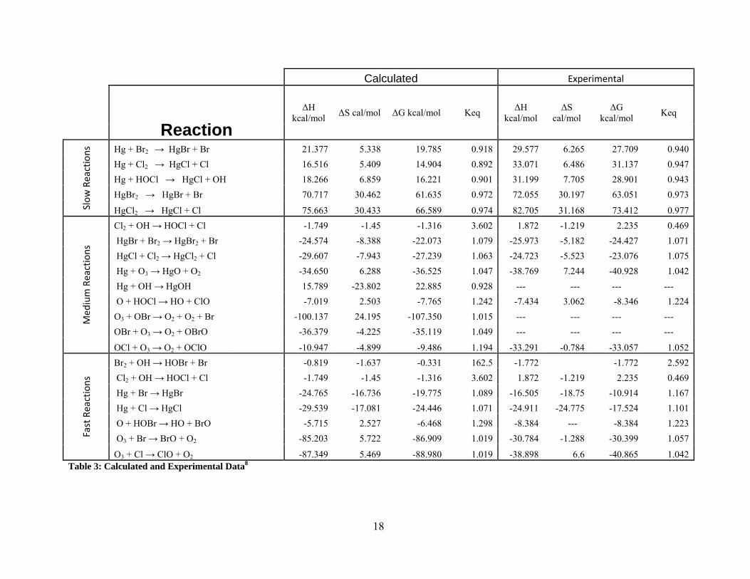
      Calculated Experimental 

 

Reaction ΔH

kcal/mol ΔS cal/mol ΔG kcal/mol Keq ΔH kcal/mol

ΔS cal/mol

ΔG kcal/mol Keq

 

Slow

 Reactions  Hg + Br2 → HgBr + Br    21.377 5.338 19.785 0.918 29.577 6.265 27.709 0.940

Hg + Cl2 → HgCl + Cl    16.516 5.409 14.904 0.892 33.071 6.486 31.137 0.947Hg + HOCl → HgCl + OH    18.266 6.859 16.221 0.901 31.199 7.705 28.901 0.943HgBr2 → HgBr + Br    70.717 30.462 61.635 0.972 72.055 30.197 63.051 0.973

HgCl2 → HgCl + Cl    75.663 30.433 66.589 0.974 82.705 31.168 73.412 0.977

Med

ium Reactions 

Cl2 + OH → HOCl + Cl    -1.749 -1.45 -1.316 3.602 1.872 -1.219 2.235 0.469 HgBr + Br2 → HgBr2 + Br    -24.574 -8.388 -22.073 1.079 -25.973 -5.182 -24.427 1.071 HgCl + Cl2 → HgCl2 + Cl    -29.607 -7.943 -27.239 1.063 -24.723 -5.523 -23.076 1.075 Hg + O3 → HgO + O2    -34.650 6.288 -36.525 1.047 -38.769 7.244 -40.928 1.042 Hg + OH → HgOH    15.789 -23.802 22.885 0.928 --- --- --- --- O + HOCl → HO + ClO    -7.019 2.503 -7.765 1.242 -7.434 3.062 -8.346 1.224O3 + OBr → O2 + O2 + Br    -100.137 24.195 -107.350 1.015 --- --- --- --- OBr + O3 → O2 + OBrO    -36.379 -4.225 -35.119 1.049 --- --- --- ---

OCl + O3 → O2 + OClO    -10.947 -4.899 -9.486 1.194 -33.291 -0.784 -33.057 1.052

Fast Reactions 

Br2 + OH → HOBr + Br    -0.819 -1.637 -0.331 162.5 -1.772 -1.772 2.592 Cl2 + OH → HOCl + Cl    -1.749 -1.45 -1.316 3.602 1.872 -1.219 2.235 0.469 Hg + Br → HgBr    -24.765 -16.736 -19.775 1.089 -16.505 -18.75 -10.914 1.167 Hg + Cl → HgCl    -29.539 -17.081 -24.446 1.071 -24.911 -24.775 -17.524 1.101 O + HOBr → HO + BrO    -5.715 2.527 -6.468 1.298 -8.384 --- -8.384 1.223 O3 + Br → BrO + O2    -85.203 5.722 -86.909 1.019 -30.784 -1.288 -30.399 1.057

O3 + Cl → ClO + O2    -87.349 5.469 -88.980 1.019 -38.898 6.6 -40.865 1.042Table 3: Calculated and Experimental Data8

18

Species Bond Length 

Bond Angle 

Vibrational Frequencies 

Br2 2.333 180 310.34

BrO 1.763 180 677.36

Cl2 2.056 180 508.10

ClO 1.626 180 792.97

HgBr 2.614 180 166.53

HgBr2 2.464 180 59.94 2.464 --- 59.94

--- --- 201.58

HgCl 2.487 180 256.09

HgCl2 2.338 180 81.90 2.338 --- 81.90

--- --- 312.98

HgO 1.964 180 534.11

HgOH 1.656 180 508.61 2.058 --- 509.35

--- --- 527.17

HOBr 0.968 103.7367 604.73 1.872 --- 1207.93

--- --- 3736.41

HOCl 0.969 103.6662 693.47 1.736 --- 1296.60

--- --- 3727.56

O2 1.205 --- 1641.19

O3 1.341 167.9463 -390.72 1.340 --- 585.70

--- --- 763.71

OBrO 1.925 180 506.76 1.925 180 ---

OClO 1.817 180 491.38 1.817 180 ---

OH 0.976 180 3650.17 Table 4: Species Bond Length, Angle and Vibrational Frequencies

19

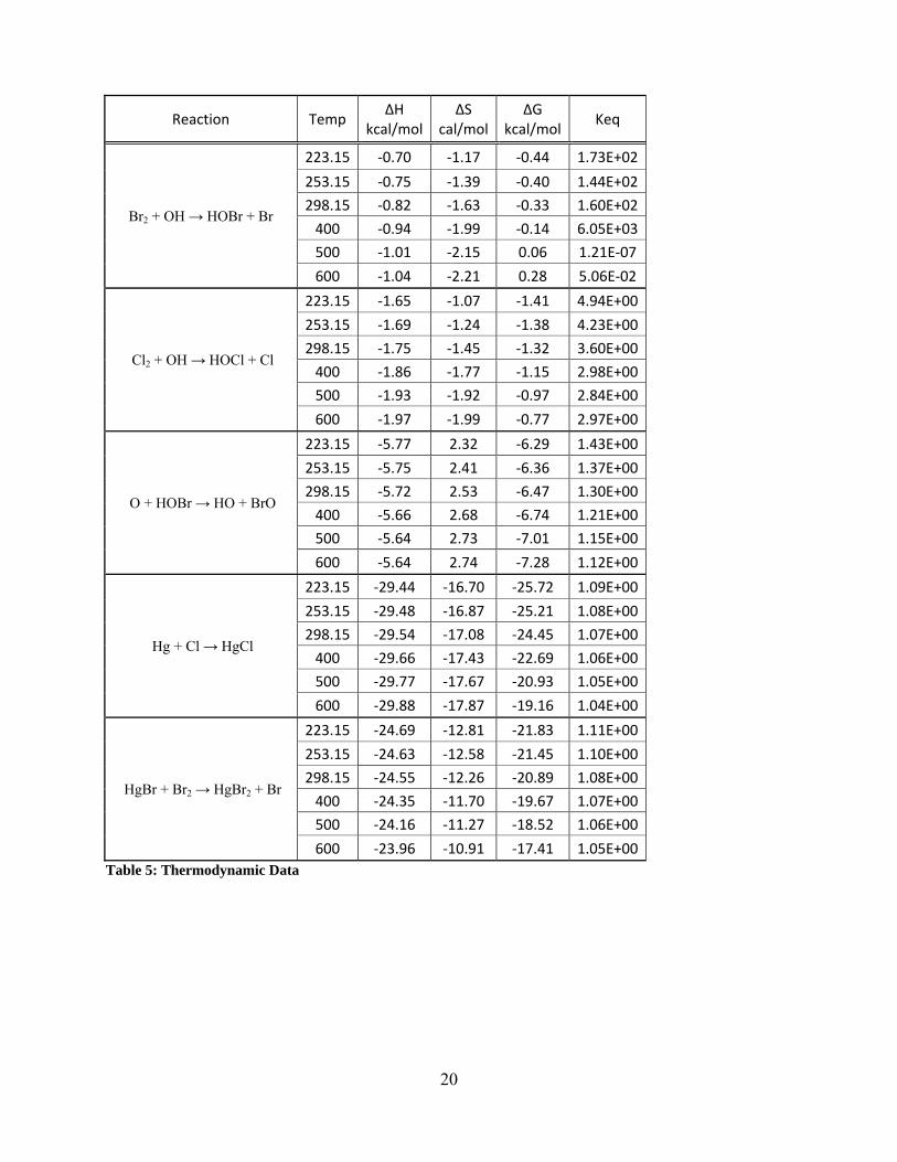
Reaction  Temp ΔH 

kcal/molΔS 

cal/molΔG 

kcal/mol Keq 

Br2 + OH → HOBr + Br

223.15  ‐0.70  ‐1.17  ‐0.44  1.73E+02 

253.15  ‐0.75  ‐1.39  ‐0.40  1.44E+02 

298.15  ‐0.82  ‐1.63  ‐0.33  1.60E+02 

400  ‐0.94  ‐1.99  ‐0.14  6.05E+03 

500  ‐1.01  ‐2.15  0.06  1.21E‐07 

600  ‐1.04  ‐2.21  0.28  5.06E‐02 

Cl2 + OH → HOCl + Cl

223.15  ‐1.65  ‐1.07  ‐1.41  4.94E+00 

253.15  ‐1.69  ‐1.24  ‐1.38  4.23E+00 

298.15  ‐1.75  ‐1.45  ‐1.32  3.60E+00 

400  ‐1.86  ‐1.77  ‐1.15  2.98E+00 

500  ‐1.93  ‐1.92  ‐0.97  2.84E+00 

600  ‐1.97  ‐1.99  ‐0.77  2.97E+00 

O + HOBr → HO + BrO

223.15  ‐5.77  2.32  ‐6.29  1.43E+00 

253.15  ‐5.75  2.41  ‐6.36  1.37E+00 

298.15  ‐5.72  2.53  ‐6.47  1.30E+00 

400  ‐5.66  2.68  ‐6.74  1.21E+00 

500  ‐5.64  2.73  ‐7.01  1.15E+00 

600  ‐5.64  2.74  ‐7.28  1.12E+00 

Hg + Cl → HgCl

223.15  ‐29.44  ‐16.70  ‐25.72  1.09E+00 

253.15  ‐29.48  ‐16.87  ‐25.21  1.08E+00 

298.15  ‐29.54  ‐17.08  ‐24.45  1.07E+00 

400  ‐29.66  ‐17.43  ‐22.69  1.06E+00 

500  ‐29.77  ‐17.67  ‐20.93  1.05E+00 

600  ‐29.88  ‐17.87  ‐19.16  1.04E+00 

HgBr + Br2 → HgBr2 + Br

223.15  ‐24.69  ‐12.81  ‐21.83  1.11E+00 

253.15  ‐24.63  ‐12.58  ‐21.45  1.10E+00 

298.15  ‐24.55  ‐12.26  ‐20.89  1.08E+00 

400  ‐24.35  ‐11.70  ‐19.67  1.07E+00 

500  ‐24.16  ‐11.27  ‐18.52  1.06E+00 

600  ‐23.96  ‐10.91  ‐17.41  1.05E+00 Table 5: Thermodynamic Data

20

21

Reaction  Temp ΔH 

kcal/molΔS 

cal/molΔG 

kcal/mol Keq 

HgCl + Cl2 → HgCl2 + Cl

223.15  ‐29.77  ‐8.56  ‐27.86  1.08E+00 

253.15  ‐29.70  ‐8.29  ‐27.60  1.07E+00 

298.15  ‐29.61  ‐7.94  ‐27.24  1.06E+00 

400  ‐29.39  ‐7.32  ‐26.46  1.05E+00 

500  ‐29.18  ‐6.86  ‐25.75  1.04E+00 

600  ‐28.98  ‐6.48  ‐25.09  1.03E+00 

Hg + O3 → HgO + O2

223.15  ‐34.70  6.11  ‐36.06  1.06E+00 

253.15  ‐34.68  6.20  ‐36.24  1.06E+00 

298.15  ‐34.65  6.29  ‐36.53  1.05E+00 

400  ‐34.62  6.37  ‐37.17  1.03E+00 

500  ‐34.61  6.40  ‐37.81  1.03E+00 

600  ‐34.60  6.42  ‐38.45  1.02E+00 

Hg + OH → HgOH

223.15  15.92  ‐23.27  21.12  8.99E‐01 

253.15  15.86  ‐23.54  21.82  9.13E‐01 

298.15  15.79  ‐23.80  22.89  9.29E‐01 

400  15.71  ‐24.04  25.32  9.52E‐01 

500  15.70  ‐24.06  27.73  9.64E‐01 

600  15.74  ‐23.98  30.13  9.73E‐01 

O + HOCl → HO + ClO

223.15  ‐7.07  2.29  ‐7.59  1.35E+00 

253.15  ‐7.05  2.39  ‐7.66  1.30E+00 

298.15  ‐7.02  2.50  ‐7.77  1.24E+00 

400  ‐6.96  2.66  ‐8.03  1.17E+00 

500  ‐6.94  2.73  ‐8.30  1.13E+00 

600  ‐6.93  2.74  ‐8.57  1.10E+00 

HgBr2 → HgBr + Br

223.15  70.73  34.47  63.03  9.65E‐01 

253.15  70.71  34.42  62.00  9.68E‐01 

298.15  70.69  34.34  60.45  9.72E‐01 

400  70.62  34.14  56.97  9.78E‐01 

500  70.54  33.97  53.56  9.81E‐01 

600  70.46  33.81  50.17  9.83E‐01 Table 6: Thermodynamic Data Cont.

APPENDIX B: FIGURES

-250

-200

-150

-100

-50

0

0 0.001 0.002 0.003 0.004 0.005 0.006 0.007

1/T

Ln (K)

Hg + Cl ‐‐> HgCl Hg + Br ‐‐> HgBr

HgCl2 ‐‐> HgCl + Cl HgBr2 ‐‐> HgBr + Br

O3 + Cl ‐‐> ClO + O2 O3 + Br ‐‐> BrO + O2

Hg + Br2 ‐‐> HgBr + Br Hg + Cl2 ‐‐> HgCl  + Cl

HgBr + Br2 ‐‐> HgBr2 + Br HgCl + Cl2 ‐‐> HgCl2 + Cl

Hg + OH ‐‐> HgOH Hg + HOCl ‐‐> HgCl + OH

Cl2 + OH ‐‐> HOCl + Cl Br2 + OH ‐‐> HOBr + Br

O + HOBr ‐‐> HO + BrO O + HOCl ‐‐> HO + ClO

Hg + O3 ‐‐> HO2 + O2 OCl + O3 ‐‐> O2 + OClO

OBr + O3 ‐‐> O2 + OBrO O3 + Br ‐‐> O2 + O2 + Br

Figure 1: All Reaction Rate Constants

22

Figure 2: Fast Reaction Rate Constants

23

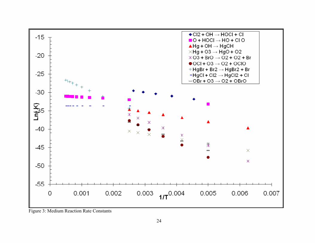
Figure 3: Medium Reaction Rate Constants

24

Figure 4: Slow Reaction Rate Constants

25

Figure 5: Equilibrium Constant Plot, Fast Reactions

26

Figure 6: Equilibrium Constant Plot, Medium Reactions

27

Figure 7: Total Column Ozone26

28

29

Figure 8: Ozone Mercury Correlation12

REFERENCES

1Abbott, M. L. (2007). Atmospheric and surface science research laboratory: Mercury in the environment. Retrieved December 6, 2007, from http://www.inl.gov/appliedgeosciences/mercury.shtml

2Adams, J.W., Cox, R.A.. Halogen chemistry of the marine boundary layer. J. Phys. IV France. Volume: 12 Issue: Pr10 Pages PR10-105 – PR10-124. 2002.

3A.M. Rankin,V. Auld and E.W. Wolff.: Frost Flowers as a Source of Fractionated Sea Salt Aerosol in

the Polar Regions.. Geophysical Research Letters. Volume 27, Number 21. Pages 3469-3472. 2000.

4Balabanov, N. B.; Peterson, K. A. A Systematic Ab Initio Study of the Structure and Vibrational

Spectroscopy of HgCl2, HgBr2, and HgBrCl. J. Chem. Phys. 2003, 119, 12271-12278. 5Becke, A.D. Density-functional thermochemistry. III. The role of exact exchange. J. Chem Phys. 1993.

98, 5648-5652

6Bernath, Peter F.. Atmospheric Chemistry Experiment (ACE): Analytical Chemistry from Orbit. Trends in Analytical Chemistry. Volume: 25, Number: 7. Pages 647-654. 2006.

7Chase, 1998Chase, M.W., Jr.,NIST-JANAF Themochemical Tables, Fourth Edition,J. Phys. Chem. Ref. Data, Monograph 9, 1998, 1-1951.

8C.T. McElroy, C.A. McLinden, and J.C. McConnell.: Evidence for bromine monoxide in the Free Troposphere during the Arctic polar sunrise.. Nature, Volume 397, 1999.

9Gaussian 03, Revision C.02, Frisch, M. J.; Trucks, G. W.; Schlegel, H. B.; Scuseria, G. E.; Robb, M. A.; Cheeseman, J. R.; Montgomery, Jr., J. A.; Vreven, T.; Kudin, K. N.; Burant, J. C.; Millam, J. M.; Iyengar, S. S.; Tomasi, J.; Barone, V.; Mennucci, B.; Cossi, M.; Scalmani, G.; Rega, N.; Petersson, G. A.; Nakatsuji, H.; Hada, M.; Ehara, M.; Toyota, K.; Fukuda, R.; Hasegawa, J.; Ishida, M.; Nakajima, T.; Honda, Y.; Kitao, O.; Nakai, H.; Klene, M.; Li, X.; Knox, J. E.; Hratchian, H. P.; Cross, J. B.; Bakken, V.; Adamo, C.; Jaramillo, J.; Gomperts, R.; Stratmann, R. E.; Yazyev, O.; Austin, A. J.; Cammi, R.; Pomelli, C.; Ochterski, J. W.; Ayala, P. Y.; Morokuma, K.; Voth, G. A.; Salvador, P.; Dannenberg, J. J.; Zakrzewski, V. G.; Dapprich, S.; Daniels, A. D.; Strain, M. C.; Farkas, O.; Malick, D. K.; Rabuck, A. D.; Raghavachari, K.; Foresman, J. B.; Ortiz, J. V.; Cui, Q.; Baboul, A. G.; Clifford, S.; Cioslowski, J.; Stefanov, B. B.; Liu, G.; Liashenko, A.; Piskorz, P.; Komaromi, I.; Martin, R. L.; Fox, D. J.; Keith, T.; Al-Laham, M. A.; Peng, C. Y.; Nanayakkara, A.; Challacombe, M.; Gill, P. M. W.; Johnson, B.; Chen, W.; Wong, M. W.; Gonzalez, C.; and Pople, J. A.; Gaussian, Inc., Wallingford CT, 2004.

10Hedgecock, Ian M., Pirrone, Nicola, and Gensini, Mario. The Interaction Between Sea Salt Aerosol, Halogen Species in the MBL and Mercury. CNR-Istituto sull'Inquinamento Atmosferico. http://ies.jrc.cec.eu.int/Units/cc/events/torino2001/torinocd/Documents/Marine/MP19.htm Accessed: January

11Hov, Oystein; Shepson, Paul; Wolff, Eric. The Chemical Composition of the Polar Atmosphere-The IPY Contribution. WMO Bulletin Volume: 56 Number: 4. Pages 263-269. October 2007.

30

12J. Sommar, I.Wangberg T. Berg, K. Gardfeldt, J. Munthe, A. Richter, A. Urba, F. Wittrock, and W. H. Schroeder. Circumpolar transport and air-surface exchange of atmospheric mercury at Ny-A° lesund (79_ N), Svalbard, spring 2002. Atmos. Chem. Phys. Volume: 7, Pages: 151-166. 2007.

13Kolker, A., & Engle, M. (2007). Mercury in coal. Retrieved December 6, 2007, from http://energy.er.usgs.gov/health_environment/mercury/mercury_coal.htm

tml

14Kolker, A., & Engle, M. (2007). Investigating atmospheric mercury with the U.S. geological survey mobile mercury laboratory

15Kolker, A., & Engle, M. (2007). Atmospheric Mercury Speciation,Retrieved December 6, 2007, from http://energy.er.usgs.gov/health_environment/mercury/mercury_atmospheric.h

16Kolker, A., Engle, M. & Belkin, H. (2007). Mercury emissions from china. Retrieved December/06, 2006, from http://energy.er.usgs.gov/health_environment/mercury/mercury_china_emissions.html

17Lee, C.; Yang, W.; Parr, R. G. Development of the Colle-Salvetti correlation-energy formula into a functional of the electron density. Phys. Rev. B. 1998, 37, 785-789

18Lee, S. J., Seo, Y., Jurng, J., Hong, J., Park, J., Hyun, J. E., et al. (2004). Mercury emissions from selected stationary combustion sources in Korea. Science Direct, 325, 155-161.

19Molina, M., Molina L., Kolb, C. E.. Gas-Phase and Heterogeneous Chemical Kinetics of the Troposphere and Stratosphere. Annu. Rev. Phys. Chem.. 1996. 47:327-67

20Mukherjee, A.B., Zevenhoven, R.. Mercury in coal ash and its fate in the Indian subcontinent: A synoptic review. Science of the Total Environment. Volume: 368, Pages: 384-392. 2006.

21Nriagu, J., & Becker, C. (2003). Volcanic emissions of mercury to the atmospher: Global and regional inventories. The Science of the Total Environment, 304, 3-12.

22Pirrone, N., Costa, P., Pacyna, J. M., & Ferrara, R. (2001). Mercury emissions to the atmosphere from natural and anthropogenic sources in the Mediterranean region. Atmospheric Environment, 35, 2997-3006.

23Sander, R., Keene, W. C., Pszenny, A. A. P., Arimoto, R., Ayers, G. P., Baboukas, E., Cainey, J. M., Crutzen, P. J., Duce, R. A., Hönninger, G., Huebert, B. J., Maenhaut, W., Mihalopoulos, N., Turekian, V. C., and Van Dingenen, R.: Inorganic bromine in the marine boundary layer: a critical review, Atmos. Chem. Phys., 3, 1301-1336, 2003.

24Schiermeier, Q. (2007). Chemists poke holes in ozone theory. Retrieved December, 2007, from http://www.ncas.ac.uk/news/stories/chemists_poke_holes_in_ozone_hole.html

25Stevens, W. J.; Krauss, M. Relativistic Compact Effective Core Potentials and Efficient, Shared-Exponent Basis Sets for the Third-, Fourth-, and Fifth-Row Atoms. Can. J. Chem. 1992, 70, 612-630

31

32

26U.S. Department of Commerce-National Oceanic and Atmospheric Administration-Earth System Research Laboratory-Global Monitoring Division. (2007). South pole total column ozone. Retrieved January 05, 2008, from http://www.esrl.noaa.gov/gmd/dv/spo_oz/spototal.html

27U. S. EPA (2007). Controlling Power Plant Emissions: Overview. Retrieved February 25, 2008. from:

http://www.epa.gov/hg/control_emissions/index.htm 28W. R. Simpson, R. von Glasow, K. Riedel, P. Anderson, P. Ariya, J. Bottenheim, J. Burrows, L. J.

Carpenter, U. Frieß, M. E. Goodsite, D. Heard, M. Hutterli, H.-W. Jacobi, L. Kaleschke, B. Neff, J. Plane, U. Platt, A. Richter, H. Roscoe, R. Sander, P. Shepson, J. Sodeau, A. Steffen, T. Wagner, and E.Wolff.: Halogens and their role in the polar boundary-layer ozone depletion. Atmos. Chem. Phys., 7, 4375-4418, 2007.

29Wang, D., He, L., Wei, S., & Feng, X. (2006). Estimation of mercury emission from different sources to atmosphere in chongqing, china. Science Direct, (366), 722-728.

30Wiedinmyer, C., & Friedli, H. (2007). Mercury emissions estimates from fires: An initial inventory for the United States. Environment Science Technology, 41(23), 8092-8098.

31Yudovich, Y. E., & Ketris, M. P. (2005). Mercury in coal: A review part 2. coal use and environmental problems. Science Direct, 62, 135.

32Yung, Y. L., Pinto, J. P., Watson, R. T., and Sander, P.: Atmospheric bromine and ozone perturbations in the lower stratosphere. J. Atmos. Sci., 37, 339-353, 1980.

33Zheng, Liugen, Guijian, Liu, Chou, Chen-Lin. The distribution, occurrence and environmental effect of

mercury in Chinese coals. Science of the Total Environment. Volume: 384, Pages 374-383. 2007. 34Zheng, L., Lui, G., & Chou, C. (2007). The distribution, occurrence and environmental effect

of mercury in Chinese coals. Science Direct, 384, 374.