Embed Size (px)
Citation preview

Comparison of Two Planning Methods for Heterogeneity Correction in Planning Total Body Irradiation
Emily Elizabeth Flower
BAppSci (Medical Biophysics and Instrumentation)
School of Applied Sciences
RMIT University
December 2005
I

Statement Except where due acknowledgement or reference has been made, the work in this
thesis is original. To the best of my knowledge no other person’s work has been used
without due acknowledgement. This work has not been previously submitted in whole
or part to qualify for any other degree. The experimentation and analysis of data are
largely my own work, with the support and constructive assistance of my supervisors.
This thesis is the result of work completed after the official commencement of this
degree.
Emily Flower
December 2005
II

Acknowledgements
I would firstly like to acknowledge my supervisors, Prof Peter Johnston and Mr
Romuald Gajewski. Their support and direction have been beneficial in this project.
My fellow Medical Physicists from Westmead Hospital, particularly the Director of
Medical Physics, Mr Gary Arthur, for allowing time and resources to work on this
project and for helping with more constructive criticism. Also Miss Alison Gray who
proofread my thesis.
Mr Dennis Payne, from the Biomedical Engineering Department at Westmead
Hospital, for obtaining and machining the PerspexTM and cork inserts required for my
phantom.
I also acknowledge the working program for TLD dosimetry and TBI treatments that
already exists at Westmead Hospital, including the design of the current 2D planning
protocol, treatment protocol and TBI cradle design.
I thank my family and friends for their unfailing support and encouragement
throughout my studies and particularly during the preparation of this thesis.
Finally, as a spirit filled Christian I acknowledge the work of God in my life. As a child
I was diagnosed as having learning difficulties and my parents were told not to
expect me to finish school. I started school with an integration aid, and my early
reports followed the predicted pattern. However, my God healed me, to the extent
that I have prepared this thesis for my Masters Degree. Having the Holy Spirit in my
life also is a great source of strength and comfort in my life. I thank God for my life
and the opportunity to complete this degree.
III

Summary Total body irradiation (TBI) is often used as part of the conditioning process prior to
bone marrow transplants for diseases such as leukemia. By delivering radiation to
the entire body, together with chemotherapy, tumour cells are killed and the patient is
also immunosupressed. This reduces the risk of disease relapse and increases the
chances of a successful implant respectively.
TBI requires a large flat field of radiation to cover the entire body with a uniform dose.
However, dose uniformity is a major challenge in TBI. (AAPM Report 17) The ICRU
report 50 recommends that the dose range within the target volume remain in the
range of –5% to +7%. Whilst it is generally accepted that this is not possible for TBI,
it is normally clinically acceptable that ±10% of the prescribed dose to the whole body
is sufficiently uniform, unless critical structures are being shielded.
TBI involves complex dosimetry due to the large source to treatment axis distance
(SAD), dose uniformity and flatness over the large field, bolus requirements, extra
scatter from the bunker walls and floor and large field overshoot. There is also a lack
of specialised treatment planning systems for TBI planning at extended SAD.
TBI doses at Westmead Hospital are prescribed to midline. Corrections are made for
variations in body contour and tissue density heterogeneity in the lungs using bolus
material to increase dose uniformity along midline.
Computed tomography (CT) data is imported into a treatment planning system. The
CT gives information regarding tissue heterogeneity and patient contour. The
treatment planning system uses this information to determine the dose distribution.
Using the dose ratio between plans with and without heterogeneity correction the
effective chest width can be calculated. The effective chest width is then used for
calculating the treatment monitor units and bolus requirements.
In this project the tissue heterogeneity corrections from two different treatment
planning systems are compared for calculating the effective chest width. The
treatment planning systems used were PinnacleTM, a 3D system that uses a
convolution method to correct for tissue heterogeneity and calculate dose. The other
IV

system, RadplanTM, is a 2D algorithm that corrects for tissue heterogeneity using a
modified Batho method and calculates dose using the Bentley – Milan Algorithm.
Other possible differences between the treatment planning systems are also
discussed.
An anthropomorphic phantom was modified during this project. The chest slices were
replaced with PerspexTM slices that had different sized cork and PerspexTM inserts to
simulate different lung sizes. This allowed the effects of different lung size on the
heterogeneity correction to be analysed. The phantom was CT scanned and the
information used for the treatment plans.
For each treatment planning system and each phantom plans were made with and
without heterogeneity corrections. For each phantom the ratio between the plans
from each system was used to calculate the effective chest width. The effective chest
width was then used to calculate the number of monitor units to be delivered.
The calculated dose per monitor unit at the extended TBI distance for the effective
chest width from each planning system is then verified using thermoluminescent
dosimeters (TLDs) in the unmodified phantom. The original phantom was used for
the verification measurements as it had special slots for TLDs.
The isodose distributions produced by each planning system are then verified using
measurements from Kodak EDR2 radiographic film in the anthropomorphic phantom
at isocentre. Further film measurements are made at the extended TBI treatment
SAD.
It was found that only the width of the lungs made any significant difference to the
heterogeneity correction for each treatment planning system. The height and depth of
the lungs will affect the dose at the calculation point from changes to the scattered
radiation within the volume. However, since the dose from scattered radiation is only
a fraction of that from the primary beam, the change in dose was not found to be
significant.
This is because the calculation point was positioned in the middle of the lungs, so the
height and depth of the lungs didn’t affect the dose at the calculation point.
V

The dose per monitor unit calculated using the heterogeneity correction for each
treatment planning system varied less than the accuracy of the TLD measurements.
The isodose distributions measured by film showed reasonable agreement with those
calculated by both treatment planning systems at isocentre and a more uniform
distribution at the extended TBI treatment distance.
The verification measurements showed that either treatment planning system could
be used to calculate the heterogeneity correction and hence effective chest width for
TBI treatment planning.
VI

TABLE OF CONTENTS
CHAPTER ONE – INTRODUCTION …………………………………………………….11
CHAPTER ONE – INTRODUCTION...........................................................................1
CHAPTER ONE – INTRODUCTION...........................................................................1
CHAPTER TWO – LITERATURE REVIEW................................................................6
CLINICAL ASPECTS......................................................................................................................6 TBI DELIVERY TECHNIQUES .......................................................................................................8 TISSUE COMPENSATION.............................................................................................................11 BEAM DATA ..............................................................................................................................11 TREATMENT PLANNING .............................................................................................................16 DOSE DISTRIBUTIONS ................................................................................................................25 LUNG DOSES .............................................................................................................................26 DOSE VERIFICATION - PHANTOM MEASUREMENTS ..................................................................27 DOSE VERIFICATION – INVIVO DOSIMETRY...............................................................................28 THERMOLUMNISCIENT DOSIMETRY...........................................................................................29 FILM DOSIMETRY ......................................................................................................................30
CHAPTER THREE – METHODS ..............................................................................32
PHANTOM DESIGN ....................................................................................................................32 MEASUREMENTS OF PHANTOM ...............................................................................................33 PRESCRIPTION..........................................................................................................................34 PLANNING.................................................................................................................................34 BEAM PARAMETERS ..................................................................................................................35 POINT OF INTEREST AND PRESCRIPTION ....................................................................................35 REPEAT TRIAL FOR HOMOGENEOUS DENSITY CORRECTION......................................................36 ISODOSE MAPS ..........................................................................................................................36 EFFECTIVE CHEST WIDTH AND TREATMENT MONITOR UNIT CALCULATION .....................37 PHANTOM VERIFICATION – TLDS ..........................................................................................39 PHANTOM VERIFICATION – FILM ...........................................................................................42
CHAPTER FOUR – RESULTS .................................................................................44
CT TO DENSITY CALIBRATION ...................................................................................................44 RATIO DIFFERENCES: RADPLANTM AND PINNACLETM ...............................................................44 FILM DOSE RESPONSE ...............................................................................................................46 ISODOSE DISTRIBUTIONS ...........................................................................................................47
VII

CHAPTER FIVE – DISCUSSION..............................................................................52
CHAPTER SIX – CONCLUSION ..............................................................................57
REFERENCES..........................................................................................................59
VIII

LIST OF DIAGRAMS
DIAGRAM 2.1 – SHOWS SOME OF THE DELIVERY TECHNIQUES AVAILABLE FOR TBI. (SOURCED FROM AAPM REPORT 17)....................................................................................................9
DIAGRAM 2.2 – SETUP ARRANGEMENT FOR MEASUREMENT OF TPR AND TMR, WHERE D IS ANY GIVEN DEPTH AND DREF IS A FIXED REFERENCE DEPTH FOR TPR MEASUREMENTS AND DMAX
FOR TMR MEASUREMENTS................................................................................................13 DIAGRAM 2.3 – SETUP FOR BATHO DENSITY CORRECTION. .......................................................18 DIAGRAM 2.4 – ENERGY DEPOSITION KERNELS.........................................................................22 DIAGRAM 2.5 – SHOWS THE GEOMETRY FOR CONVOLUTION CALCULATION METHODS. (SOURCED
FROM METCALFE, KRON AND HOBAN, 1997)....................................................................22 DIAGRAM 3.1 – SHOWS THE RANDOTM PHANTOM, BOTH COMPLETE AND IN SECTIONS,
INCLUDING THE SLOTS FOR TLD PLACEMENT....................................................................32 DIAGRAM 3.2 – A SLICE OF THE LUNG INSERT PART OF THE ANTHROPOMORPHIC PHANTOM
MODIFICATION SHOWING THE ARRANGEMENT OF THE SMALLEST LUNG ON THE LEFT, WITH A CORK INSERT SURROUNDED BY PERSPEX INSERTS AND THE LARGEST LUNG, WITH THE CORK INSERT FROM THE SMALLER LUNG ARRANGEMENT SURROUNDED WITH CORK INSERTS, AS ALSO SEEN LOOSE ON THE SIDE. .....................................................................33
AS THE AREA OF INTEREST FOR THE PHANTOM VERIFICATION TESTING WAS NOT NEAR THE SURFACE, FOR EASE OF SETUP A BEAM SPOILER WAS NOT USED DURING EITHER PLANNING OR TREATMENT..................................................................................................................33
DIAGRAM 3.3 – PLACEMENT OF THE TLDS AT THE RED CROSSES. ............................................41 DIAGRAM 4.1 – THE HOUNSFIELD CALIBRATION FOR DENSITY USED BY THE PLANNING SYSTEMS.
THE PINNACLETM SYSTEM USES CT NUMBERS SO THESE HAVE BEEN CONVERTED TO HOUNSFIELD NUMBER FOR DISPLAY. .................................................................................44
DIAGRAM 4.2 – THE CALIBRATION FILM USED TO CONVERT OPTICAL DENSITY TO DOSE. ..........46 DIAGRAM 4.3 – THE CALIBRATION CURVE USED TO CONVERT OPTICAL DENSITY TO DOSE. .......47 DIAGRAM 4.4 – ISODOSE DISTRIBUTION IN THE TRANSVERSE PLANE AT 100 CM SAD
CALCULATED BY PINNACLETM. ..........................................................................................48 DIAGRAM 4.5 – ISODOSE DISTRIBUTION IN THE TRANSVERSE PLANE AT 100 CM SAD
CALCULATED BY RADPLANTM............................................................................................48 DIAGRAM 4.6 – MEASURED ISODOSE DISTRIBUTION FROM FILM AT AND SAD OF 100 CM IN
RANDOTM. .......................................................................................................................49 DIAGRAM 4.7 – MEASURED ISODOSE DISTRIBUTION FROM FILM AT EXTENDED SAD OF 400 CM
IN RANDOTM....................................................................................................................49 DIAGRAM 4.8 – RANDOTM PINNACLETM ISODOSE DISTRIBUTION WITH HETEROGENEITY
CORRECTION AT 400 CM SAD. ..........................................................................................50 DIAGRAM 4.9 – RANDOTM PINNACLETM ISODOSE DISTRIBUTION WITHOUT HETEROGENEITY
CORRECTION AT 100 CM SAD. ..........................................................................................50 DIAGRAM 4.10 – RANDOTM RADPLANTM ISODOSE DISTRIBUTION WITHOUT HETEROGENEITY
CORRECTION AT 100 CM SAD. ..........................................................................................51
IX

LIST OF TABLES
TABLE 4.1 – THE EFFECTIVE CHEST WIDTHS CALCULATED USING THE RATIOS BETWEEN
HETEROGENEITY AND HOMOGENEITY CALCULATIONS FROM PINNACLETM AND
RADPLANTM FOR DIFFERENT PHANTOMS. .........................................................................45
TABLE 4.2 – DOSE (GY) PER MONITOR UNIT AT THE EXTENDED TBI SAD OF 400 CM AS
CALCULATED USING THE RATIOS FROM RADPLANTM AND PINNACLETM AND MEASURED
USING TLDS. ....................................................................................................................45
X

Chapter One – Introduction Radiation Oncology is a branch of medicine dedicated to the use of ionising radiation
to destroy cancer cells. For most cases, the cancer is a solid tumour and the
radiation dose is delivered to the tumour and any likely sites of spread such as lymph
nodes, as a localised treatment. Systemic treatments such as chemotherapy are also
available. For systemic diseases such as leukaemia, localised treatment is not an
option, as the entire body requires treatment.
Part of the treatment available for diseases such as leukaemia is a bone marrow
transplant (BMT). Total body irradiation (TBI) is a part of the treatment given prior to
a bone marrow transplant. TBI involves the use of megavoltage photon beams to
deliver radiation to the entire body. Historically gamma ray beams from a Cobalt – 60
source were used but now linear accelerators are used for TBI throughout Australia.
The radiation destroys the tumour cells and suppresses the immune system,
reducing the risk of disease relapse and increasing the chance that the transplant will
be successful.
BMT success rates are such that “patients with acute myeloid leukemia transplanted
in first remission can now expect an approximately 50 to 60% likelihood of long-term
disease-free survival. Similar probabilities are also achievable after transplantation of
adults with acute lymphoblastic leukemia in first remissions. Probability of relapse
correlates with remission status at the time of the transplant, ranging from 20% in first
remission to 60% with more advanced disease. Long-term survival for patients with
chronic myelocytic leukemia who receive BMT in the phase of remission is 60 to
70%”. (Merck Manual 2005)
As with all radiation therapy the treatment process begins with collection of general
linear accelerator data during commissioning, which is used for treatment planning.
Then the patient data required for dose calculation is collected. This can involve
physical measurements of patient size and contour, radiographic imaging and/or
computed tomography (CT) scanning. How the patient will be positioned during
treatment is also determined at this time, as well as the position of any accessories
used during treatment, such as the beam spoiler. This process is known as patient
simulation.
1

The next stage for all radiation therapy treatments is known as treatment planning.
During planning the beam arrangement and fluence is determined and the number of
monitor units to be delivered so the prescribed dose to be given is calculated.
Evaluation tools such as isodose map and dose volume histograms can be used to
verify the target is receiving the correct dose and that organs at risk are receiving an
acceptable dose, i.e. the dose to critical structures is as low as possible.
Different methods can be used to calculate dose for radiation treatment. This thesis
investigates whether there are any differences between two planning methods for
TBI at extended distances. The two methods are a 2D planning Bentley – Milan
algorithm with modified Batho heterogeneity correction method and 3D planning
convolution method. This included testing any differences due to different lung sizes.
The results were verified with thermoluminescent dosimeters (TLD) and film
measurements in an anthropomorphic phantom.
Anthropomorphic phantoms can be used to verify the dose distribution and absolute
doses at points predicted by treatment planning systems. These measurements are
made using ionising radiation detectors such as radiographic film and TLDs. This
verification process evaluates the different methods of calculating dose for radiation
treatment.
Only after the accuracy of a dose calculation method has been verified with such
measured data can this method be used to calculate the number of monitor units for
each beam of a patient treatment.
During treatment the patient is setup the same way as they were positioned during
the patient simulation process and the treatment is delivered as planned. Invivo
dosimetry, where measurements are made with detectors on or inside the patient
during treatment, is another verification method. Invivo dosimetry can be used to
determine the accuracy of the entire treatment chain from simulation to treatment as
described above.
2

In chapter two a literature review is completed, to give a background to this research
project. This begins by covering the clinical aspects of TBI, including the short term
and long term side effects of TBI.
Some of the methods used for delivering TBI are discussed in chapter two, including
the requirements of the delivery systems. The various methods for tissue
compensation such as bolus material or metal compensators are also discussed.
These can either compensate for variations in patient shape or for low density
regions, to ensure the same effective pathlength to the patient’s midline.
For radiation therapy treatment planning to occur, parameters about the treatment
beam, such as its profile and percentage depth dose curve, as well various factors
related to beam scatter need to be determined. The beam data required for TBI
treatment planning is discussed.
Methods for planning TBI treatment are discussed, including tissue density
heterogeneity corrections. The algorithms used by both treatment planning systems
for calculating radiation dose are also described. Factors that influence the overall
dose distribution and more specifically lung dosimetry during TBI are also discussed.
The lung is of particular interest because lung tissue has a lower density than muscle
tissue so offers less attenuation to radiation, affecting the dosimetry. Lung tissue is
also radiation sensitive as demonstrated by one of most serious morbidities from TBI,
radiation pneumonitis.
Methods for verifying the calculated dose are also described. Some of the
characteristics of TLDs and films, two of the most commonly used dosimeters for
verification measurements, are also discussed.
In chapter three the project methodology is discussed. A phantom was designed by
modifying an anthropomorphic phantom with a specially developed chest insert to
replace the original phantom chest slices. This enabled different lung sizes to be
simulated. This phantom was then scanned with its different lung sizes.
The CT datasets were then used to create plans for the various different lung sizes.
RadplanTM calculates dose using the Bentley – Milan algorithm and corrects for
3

heterogeneities using a modified Batho technique. PinnacleTM (ADAC laboratories,
Milpitas, CA) uses a convolution method to calculate dose distributions.
For each treatment planning system the plans were repeated without tissue
heterogeneity corrections. The ratio between the plan with heterogeneity correction
and without for each system was then used to calculate the effective chest width. The
effective chest width was then used to calculate the number of monitor unitFs.
To verify the planning processes worked as expected, plans were made using the
unmodified RANDOTM phantom with TLD slots. The planned point doses were
verified by placing TLDs within the phantom and delivering a treatment at the
extended TBI SAD of 400 cm to the phantom as planned. Comparisons were made
between the measured dose and the planned dose.
Kodak EDR2 radiographic film was also placed into the phantom to measure the
delivered dose distribution. This measured dose distribution was then compared to
the planned dose distributions from each planning system. This process was
repeated at 100 cm SAD (isocentre) and the extended TBI treatment distance of 400
cm.
Chapter four presents the results calculated using data from the treatment planning
systems. The effective chest width is calculated using the ratio between the monitor
units from the treatment planning systems with and without heterogeneity correction.
The dose per monitor unit verification measurements with TLDs and dose distribution
verification measurements with radiographic film are also presented.
Chapter five discusses the results of the planning studies and the phantom
verification measurements. It also discusses the errors and uncertainties pertaining
to this study and clinical TBI treatments. Suggestions are made for future work.
Chapter six offers the conclusions of the study. Whilst a difference was calculated,
this difference was smaller than the accuracy of the TLD measurements. Hence no
significant difference could be detected between the two planning methods. The film
measurements showed reasonable agreement with both planning systems at 100 cm
4

SAD and significant differences at 400 cm SAD. Either method could be used
clinically.
5
Chapter Two – Literature Review
Clinical Aspects
TBI with megavoltage photon beams is a radiotherapeutic procedure that is used for
the treatment of haematological disorders and disseminated malignancies such as
acute leukaemia, lymphomas or aplastic anaemia. It is part of the cytoreductive
conditioning program prior to a bone marrow or stem cell transplants, along with
chemotherapy. (AAPM report 17; Harden, 2001)
TBI helps remove tumour cells from the body and also results in adequate
immunosuppression for a successful graft. (Galvin, 1980; Kim, 1980) This is due to
the ablation of normal hemopoietic and lymphoid cells, which helps facilitate
engraftment of the new cells. With TBI treatments there are no sanctuary sites (due
to radiation penetration throughout entire body) or evolution of clonal resistance. It is
also likely that chemoresistant leukemic cells will remain radiosensitive (Doughty,
1987).
As with all treatment modalities, it is desirable to have the maximum possible
therapeutic ratio, ie, high disease control with minimal normal tissue toxicity,
especially to critical tissues. (Obcemea, 1992)
Short-term side effects of TBI include mucositis, alopecia, dysphagia, diarrhoea,
parotitis, erythema, pneumonitis, veno-occlusive disease and all the attendant risks
of prolonged pancytopaenia. The long-term risks include ophthalmological sequelae
(cataracts), endocrinological sequelae (reduced pituitary function), neurological
sequelae, infertility and increased risk of secondary malignancies. (Harden, 2001;
Quast, 1987) Following the BMT there is also a risk of graft versus host disease.
(Yuille, 1983) The dose tolerance of various different normal tissues for non-
stochastic radiation effects is discussed in the ICRP report 44.
TBI was originally given as a single fraction (Harden, 2001) but side effects can be
reduced with fractionated treatments, based on radiobiology principles of preferential
6

normal tissue repair. Studies have found that fractionated TBI can reduce side effects
whilst still producing good anti-leukemic outcomes. (Cosset, 1994; Shank, 1983)
Dose uniformity is a major challenge in TBI. (AAPM Report 17) Under-dosages will
increase the risk of relapse whilst overdose, especially to critical organs (lungs, eye
lens etc), will increase toxicity. According to the ICRU report 50 the dose range within
the target volume should remain in the range of –5% to +7%. So for TBI the ideal
situation is that the whole body including the skin receives a dose within –5% and
+7% of the prescribed dose. Whilst it is generally accepted that this is not possible
for TBI , the effect on the clinical outcome is not known. (Galvin, 1980; Vollans, 2000)
Typically ±10% of the prescribed dose to the whole body provides clinically
acceptable dose uniformity, with the possible exception of the extremities and other
non-critical structures. (Khan, 2003)
Prescriptions tend to be in the range of 5 to 14 Gy, in up to 8 fractions, often treated
twice daily. TBI reduces the number of malignant stem cells by a factor of 10 for each
1.5 to 2 Gy. (Quast, 1987) ICRU 29 recommends a prescription point as being
central and at a depth of half the patient’s thickness. The prescription point when
used will typically be in the abdominal or pelvis region (Sanchez-Doblano, 1995),
such as the midpoint at the umbilicus level (Syh, 1992). Sometimes the prescription
will be to the entire midline or midplane. (Kim, 1980) Sometimes a lower dose rate of
5 – 10 cGy per minute at the prescription point is used. (AAPM report 17)
Radiation dose rate and fractionation schedule can affect the incidence of radiation
pneumonitis and need to be considered in the prescription. (Yuille, 1983) Dose limits
are sometimes prescribed to critical organs such as the lungs, for example, 9.6 Gy to
the lungs when the whole body doseprescription was 12 Gy. (Sanchez-Doblano,
1995, Svahn-Tapper, 1990))
Most data for radiation syndromes come from nuclear incidents and are therefore
from a single exposure. For TBI the patient will suffer from bone marrow (or
hemopoietic) syndrome. The dose should however be low enough to not cause any
concern regarding gastrointestinal or central nervous system syndromes. Following a
TBI treatment, patients can survive only if they receive a BMT.
7

TBI Delivery Techniques
There is no generally accepted technique for delivering TBI. Factors that may
influence the way in which TBI patients are treated include the size of the treatment
room, energy of the linear accelerator and availability of another linear accelerator as
a back up machine. Some centres have dedicated large field TBI irradiators in
specially designed treatment rooms but most use standard radiotherapy accelerators
for TBI. (Curran, 1989; Podgorsak, 1985; AAPM report 17) Some use single sources
of radiation, others dual (Obcemea, 1992) or multiple sources from different
directions (Sanchez-Doblano, 1995, AAPM report 17).
If using a single radiation source, such as one accelerator in a bunker, either 2 field
or 4 field techniques have been used to deliver TBI (Vollans, 2000). For the two field
techniques, they can be either opposed bilateral or anterior/posterior.
Anterior/posterior treatments are delivered with the patient in a sitting or standing
position (Harden, 2001) or lying on their side. For bilateral techniques the patient is
usually supine either lying flat or semi-reclined, often with legs flexed to reduce the
patient’s length to fit in the field. Four field techniques involve anterior, posterior and
bilateral fields. Diagram 2.1 shows some of the delivery techniques used for TBI.
TBI requires the use of a very large, uniform high-energy photon beam so the entire
body receives a uniform dose. To get such a large field size, the principle of
geometric beam divergence from the source is applied. In order to get a treatment
field large enough to treat the entire body, source to axis distances (SADs) of 3 – 5 m
are used. (Thomas, 1990)
8

Diagram 2.1 – Shows some of the delivery techniques available for TBI. (Sourced from AAPM report 17)
Various different photon energies are used for TBI, from gamma rays from a cobalt-
60 teletherapy units (1.25 MeV) through to linear accelerator beams from 4 MV to 25
MV. (Sanchez-Doblano, 1995) Cobalt-60 Teletherapy units are no longer used for
radiotherapy treatment delivery in Australia. For lateral treatments higher energies (ie
10 MV or higher) are preferred for delivering a more uniform dose distribution as the
beam needs to travel through the pelvis and shoulder regions. However, for AP/PA
treatments, 6 MV beams provide less undesirable high dose regions in the lungs.
(Ekstrand, 1997)
Linear accelerators use high frequency electromagnetic waves to accelerate
electrons through a linear accelerating tube. To produce an x-ray photon beam these
electrons hit a target made of a high Z material such as tungsten, producing
bremsstrahlung x-rays. Following the target, the beam intensity is modified by a
flattening filter. The target is thick enough to absorb most of the electrons. The beam
9

then passes through two independent ion chambers, which monitor beam output and
symmetry. Finally the beam is collimated.
There are also other techniques that use multiple parallel and adjacent beams or
moving beams or patient translation. (Sanchez-Doblano, 1995) These are often
applied if a smaller treatment distance is available. Adjacent beams from a single
accelerator, such as in diagram 2.1j, create concerns regarding complex dosimetry at
field junctions and circulating cells potentially receiving a reduced dose. Using field
junctions can also cause concern of hot spots if the beam overlap at the junction or
cold spots if there is a gap at the junction. (Rider, 1983)
To achieve a treatment field 2 m long an SAD of 5 m is required. To ensure the
patient remains in the field the collimator is rotated through 45° with the jaws opened
to the maximum aperture (usually 40 x 40 cm at 100 cm SAD). (Harden, 2001) The
TBI treatment SAD can be marked with a laser line which can be aligned to patient
midline to aid setup to treatment SAD. (Svahn-Tapper, 1990)
A low atomic number absorber (such as a PerspexTM screen) is often placed in front
of the patient, acting as a beam spoiler. This reduces the dose build up region. This
improves the dose distribution to the skin, making it more similar to the prescribed
dose. For a 10 mm spoiler placed 15 cm in front of the patient with a beam spoiler
correction factor applied at a depth of 5 cm, the depth dose increased by only 1% at
2 cm depth. At larger depths the spoiler was found not to influence the depth dose
values. (Svahn-Tapper, 1990) The surface dose also increases as beam energy
decreases, the distance between the spoiler and the patient decreases and with
increasing spoiler thickness (towards depth dose max). A 1 cm thick PerspexTM beam
spoiler for a 10 MV photon beam will increase the skin dose up to 97% of dmax.
(Sanchez-Nieto, 1997) The required thickness of the beam spoiler is dependent upon
the energy of the beam, as the position of the dmax changes with beam energy.
However the clinical effects of skin dose is not known as no systematic study has
been completed analysing this. (Kim, 1980)
10

Tissue Compensation
Some centres do not use any compensation for irregularities in patient shape.
(Vollans, 2000) If missing tissue due to contour variations of the patient is to be
accounted for, this can be achieved using either missing tissue compensators or
tissue-equivalent bolus. These compensators provide greater dose uniformity along
the body by reducing the irregularity of the body thickness. (Khan, 2003; Galvin,
1980; Khan, 1980. The compensators are placed between the source and the
patient, either in the accessory mount or are mounted onto the beam spoiler.
Bolus material placed around the patient for TBI needs to be malleable and be able
to hold a shape at room temperature, as well having a density that is soft tissue
equivalent. Strictly this refers to electron density, but physical density can be used
satisfactorily as an approximate measure of electron density for low Z materials.
Materials such as rice or bicarbonate soda are not quite as dense as tissue (AAPM
report 17) but in small bags make suitable bolus materials, although it can be hard to
control the thickness. One group designed bolus by making a compound of soft
paraffin and acrylic granules, sealed in thin elastic polyurethane bags. This then has
a putty type consistency. (Doughty, 1987) Various commercial tissue equivalent
bolus materials are also available. Bolus material can also be added under the legs
where it not only provides extra scatter but also provides support for the patient.
(Yuille, 1983) Missing tissue compensators of lead or copper can also be designed.
(Galvin, 1980) The position of the compensators can be verified with film. (Quast,
1987)
Beam Data
Treatment planning systems require beam data to be measured and inputted in order
to calculate the dose distributions for treatments. Consideration needs to be given to
the different geometry and scatter conditions for TBI when the beam data
measurements are being made. It may not be acceptable to simply extrapolate small
field data or data measured at isocentre. When using an ion chamber for beam data
measurements, care should be taken regarding cable and stem irradiation effects, as
the radiation field can cause extra current to be induced in the cable, changing the
measured current. This is of particular concern in TBI due to the large field sizes
11

used which can mean larger lengths of cable being irradiated during measurements.
(Fiorino, 2000).
Most linear accelerator monitor unit ion chambers are absolutely calibrated to provide
a machine output of 1.0 cGy/monitor unit at machine isocentre under reference
conditions. Absolute calibration is done following certain protocols such as the IAEA
TRS 398, traceable back to primary standards. For the IAEA TRS 398 protocol, the
reference conditions for 6 MV photon beams are to use water as the phantom
material, a cylindrical ionization chamber with the reference point on the central axis
of the chamber, a measurement depth of 10 g cm-1, a source to chamber distance of
100 cm and a field size of 10 cm x 10 cm. However, some centres use the dose rate
or an output factor at the extended SAD for treatment planning for TBI (Abraham,
2000). Dose is defined as “the energy absorbed from ionizing radiation per unit
mass” and has the unit of Gray (Gy). (Johns, 1983)
Output factors can be measured to determine the monitor units for extended
distances. This would require variations based on patient size and could be used to
calculate Tissue Phantom Ratios (TPR) and/or Tissue Maximum Ratios (TMRs).
However, as discussed below TMR values vary less than 1.5% for the extended SSD
compared to isocentric treatments so dose rate calibrations can also be transferred
to extended TBI SSDs. (Khan, 1994)
A TPR is defined as the ratio of absorbed dose at any given depth to the dose at the
same point at a fixed reference depth, achieved by changing the source to surface
distance. A TMR is defined the same way as TPR except the reference depth is the
depth of maximum dose. The setup arrangement for measurements of TMR and TPR
are shown in diagram 2.2.
12

ddref
Diagram 2.2 – Setup arrangement for measurement of TPR and TMR, where d is any given depth and dref is a fixed reference depth for TPR measurements and dmax for TMR measurements.
Output factors at extended distance have been measured and the largest difference
between the smallest phantom (20 x 20 cm) and largest “infinite” phantom (50 x 140
cm) was found to be 2.4% for a 6 MV beam, implying the phantom size within the
large radiation field has a minimum effect on dose rate at the reference point.
(Podgorsak, 1985)
TBI requires a beam that covers the entire patient with an adequately flat, uniform
beam. As the collimator is often rotated to 45° for TBI the profile is that of a diagonal,
which may also affect beam flatness. The TBI beam profile in the gun-target direction
should be measured in air, as it is the primary radiation component that is to be
measured, not scattered radiation. The beam uniformity decreases as SAD
increases. The useful treatment field is that which is within the 94% isodose curve
(Sanchez-Nieto, 1997). The dose profile may also include backscattered radiation
from the wall.
Varian Linear Accelerators come with flattening filter, which is a cone shaped
attenuator. This filter is designed to produce optimal flatness at 10 cm depth for 100
cm SSD. For shallower depths and along the beam diagonals, there will be an
overflattening affect, seen as “horns” on a beam profile. For TBI, these horns will be
over the body extremities, (head and feet) which may results in some dose
enhancements in these areas. This problem was reduced at one institution by the
addition of an extra TBI flattening filter. (Doughty, 1987)
Dose ratio data such as Percentage Depth Dose (PDD), TPR or TMR data should be
measured at the centre axis and at various off axis points, such as at the level of the
13

lungs. PDD data varies with patient thickness due to changes in backscatter
(Abraham, 2000, Sanchez-Nieto, 1993, Podgorsak, 1985). The PDD can be
corrected using a Backscatter Correction Factor (BCF) and Lateral Scatter Correction
Factor (LCF). The BCF corrects for lack of backscatter by applying a ratio of the PDD
with limited backscatter versus the PDD at the same point if there was infinite
backscatter. Hence as backscatter thickness increases towards an infinite thickness,
the exponential increase in backscatter tends to 1, due its definition. However, the
BCF is linear for depth as the probability of backscatter increases with the depth of
the point of measurement.
For TBI treatments close to the bunker wall, back scattered radiation from the wall as
well the patient can be seen. For smaller phantoms midline dose will be influenced
more by backscattered radiation from the wall than for larger phantoms, which should
be considered when choosing a phantom. (Svahn-Tapper, 1990)
Similarly the LCF is the ratio between a PDD at a certain point for a given cross
section versus the PDD at the point for an infinite cross section giving full lateral
scatter. As with the BCF, the LCF has linear variation with depth and exponential
variation with distance to lateral surfaces, which tends to 1 as the thickness tends
towards full lateral scatter conditions (ie almost infinite distances to the lateral
surface, providing almost infinite lateral scatter).
As the SAD increases, the PDD shifts due to the inverse square law (Metcalfe,
1997). Not considering the deviation from the Inverse Square Law (ISL) due to
changed scatter conditions, the PDD at extended distances can be approximated
using the Mayneord Factor. (AAPM report 17, Mayneord 1994) Data calculated from
100 cm SSD data using the Mayneord factor has been compared to SSD data
measured at TBI treatment SSD (in this case 455 cm) with TBI scatter conditions.
The measured and calculated data agreed to within 2.5% for several depths from 5
cm to 30 cm. (Sanchez-Nieto, 1993) This error can be as large as 6%. (AAPM report
17) Therefore measurements should be made to confirm any conversions if needed
in large beam geometry at treatment SSD.
Off axis TMR measurements can be normalised to central axis TMR measurements.
It has been found that for TMR 35 cm and 70 cm off axis the difference between
14

central axis and off axis TMRs are 1% and 4-5% respectively for large depths.
(Svahn-Tapper, 1990) This is due to changes in the energy spectrum across the
beam. For TBI this means that central axis TMR measurements are not valid in the
distal head and feet regions.
Collimator scatter factors (CSF) correct for the difference between the field size at
calibration (typically 10 cm x 10 cm) with the treatment field size, due to changes in
scatter within the linear accelerator head. The collimator scatter factor at TBI SSD
should not vary much compared to the data measured at isocentre. The data at the
two distances for field sizes larger than 25 cm x 25 cm has been found to be within
0.3% with up to 1% variation for field sizes of 10 cm x 10 cm. (Smith, 1996, Curran,
1989) Because the jaws are always set to 40 cm x 40 cm for TBI, this will not vary
significantly between the two distances. CSF can be measured with an ion chamber
in air with a cylindrical build up cap providing a build-up depth for the photon energy
being used.
The peak scatter factor (PSF) corrects for changes in the phantom for the treatment
field size as compared to the 10 cm x 10 cm field used for calibration. For
conventional radiotherapy, the phantoms used to measure the data are normally
larger than the radiation field. However, for TBI this is not the case, but rather the
phantom is significantly smaller then the radiation field. This may affect the TMR and
PSF values for TBI. The changes for PSF depend on energy but will vary less then
1%. The TMRs have been found to vary by less 1.5%. (Curran, 1989, Khan, 1980)
Due to scattered radiation from the bunker walls, floor and linear accelerator head,
discrepancies may be seen if the ISL is used to calculate the dose rate at the TBI
treatment SAD. (AAPM report 17, Rider, 1983, Van Dyk, 1987) The deviation
between the inverse square law and measured data increases with distance from the
reference. This deviation from the ISL can be fitted as a four-order polynomial, with
an error between measured and calculated data of less than 0.08%. (Sanchez-Nieto,
1997) This must also be considered in terms of the different source to point distances
within the body (Sanchez-Doblano, 1995). Other investigations have shown no
systematic deviation from the inverse square law when it is measured on the central
axis at various depths in a 30 cm3 phantom at SSD of 430 cm. (Svahn-Tapper, 1990)
Other investigations found that the inverse square predicted the measured dose to
15

within 1.5% for a variety of energies and distances. (Curran, 1989) However
deviations of up to 6% have been reported (Quast, 1987).
For TBI treatments, the equivalent square of the frontal side of the patient (from the
beam’s eye view) should be used for the field size when calculating the TMR and
PSF values as opposed to the jaw opening size. (Curran, 1989) This is because the
field size is larger then the scattering volume. This is particularly important for TMR.
The area over perimeter method is an adequate method for calculating the equivalent
square for TBI. (Podgorsak, 1985) Ideally when beam data measurements are being
made the phantom should be of similar equivalent square size to the patient so that
errors can be minimised. (Kirby, 1988)
Treatment Planning
Currently there is no commercially available treatment planning system for TBI.
Planning for TBI typically entails calculating at least one point dose. The total dose at
any point is the sum of the primary beam plus scattered radiation.
For manual calculations, the thickness of the body in the beam direction needs to be
determined at each reference point. This data is available from CT measurements
but mechanical measurements are an alternative. (Quast, 1987) An effective depth
that corrects for tissue density heterogeneities can also be used in manual
calculations. This is especially important for points near the lungs.
Some centres have also developed in house TBI treatment planning systems, using
x-ray computed tomography (CT) data. (Sanchez-Nieto, 1997) CT scans provide
anatomical information as well as density heterogeneity information. Considering the
patient’s physical parameters and anatomy can optimise the dose distribution in the
patient. (De Sapio, 1990, Quast, 1986).
To use the density heterogeneity information from a CT scan, the CT numbers need
to be calibrated to physical electron densities using an electron density calibration
phantom. Radiotherapy treatment planning systems use data tables to assign an
electron density to each pixel’s CT number or Hounsfield Unit, which is based on the
gray scale. (Khan 2003)
16

However, since at the megavoltage energies used for radiotherapy the Compton
effect is the dominant photon interaction, it is the electron density (number of
electrons per cm3 multiplied by mass density) of a material that has the most effect on
beam attenuation. However, since the number of electrons per gram of material is
very similar for many materials, (Khan, 1994) the mass density of a material may
also be used for calculating the heterogeneity corrections.
There are different methods for correcting for tissue density heterogeneities. These
methods vary from simple corrections that only correct for changes in the fluence of
the primary photon beam through to convolution methods, which also account for
scattered radiation and electron transport. Monte Carlo simulations are the most
accurate method but require long computational periods that are currently
impractical.
The effective depth can be calculated by multiplying assumed heterogeneity
correction factors for lungs by the patient’s measurements for planning purposes.
(Vollans, 2000)
deff = d – (ρrel lung x dlung) (1)
Where deff is the effective depth
d is the physical depth
ρrel lung is the relative density of the lung tissue
dlung is the physical depth taken by lung tissue
Lung density can vary between 0.15 g/cc to 0.4 g/cc as compared to water at 1.0
g/cc so heterogeneity corrections are important. By studying layered lung geometry
another investigator has found that for lung density 0.31 g/cc, a lung correction factor
of about 1.5% per centimetre of lung tissue has been found to be necessary, and that
this holds for both calculations and measurements. (Obcemea, 1992)
17

Another method uses a ratio of TARs for the physical and effective depths. (Metcalfe,
1997) This method does not take into account the relative position of the
inhomogeneity, the lateral extent of the structure or electron transport. (El-Khatib,
1986)
The Batho power law method uses TARs raised to an exponent, which depends on
tissue density. Batho originally introduced this method for calculating doses beyond a
single inhomogeneity. (Batho, 1964) This method was then extended to include
doses within the inhomogeneity (Sontag, 1991) and to calculate for a number of
inhomogeneities (Webb, 1979). This algorithm implicitly considers scattered
radiation. (Metcalfe, 1997) This method considers the relative position of the
structure. (El-Khatib, 1986) It can account for the lateral extent of the inhomogeneity
if scatter summation is also applied. (El-Khatib, 1986, Lulu, 1982) It does not
consider secondary electron transport. (El-Khatib, 1986)
Diagram 2.3 – Setup for Batho density correction.
d1
d2
ρe
ρ = 1
( )( )
1
,,
2
21
−
⎥⎦
⎤⎢⎣
⎡ +=
e
fdTARfddTAR
CFρ
(2)
Where CF is the correction factor
d1 and d2 are the depths are shown in diagram 2.3
f is the field size
18

ρe is the density of the lung tissue
For a single layered heterogeneity with a less than unit density, the dose is
underestimated within the low density region, with the largest errors near the top of
the heterogeneity. However the method shows good experimental agreement below
the heterogeneity. This method generally works well for smaller fields but the larger
the field the larger the error, due to the increase in scatter affecting the percentage
depth dose curve. (Metcalfe, 1997)
The equivalent TAR method uses multi slice CT information to account for scattered
radiation. It uses ratios of TARs depending on effective beam radius (to account for
scattered radiation) and effective depth (correcting for primary beam). (Metcalfe,
1997) This method considers the relative position of the inhomogeneity and the
lateral extent of the inhomogeneity but does not consider secondary electron
transport. (El-Khatib, 1986) In comparison with measured data (when the field is
large enough for electronic equilibrium) this method gives accurate results, which
implies that it adequately models scatter dose. (Metcalfe, 1997)
The differential Scatter-Air Ratio method takes the primary dose and then adds
scatter radiation. The scatter can be calculated either assuming homogeneity or
correcting for heterogeneity by considering the attenuation of the primary beam for
each scatter element or including the attenuation of scattered photons in their path to
the calculation site. (Metcalfe, 1997) This method considers the relative position of
the inhomogeneity and the lateral extent of the inhomogeneity but does not consider
secondary electron transport. (El-Khatib, 1986) A similar method is the delta volume
method. (Metcalfe, 1997)
Although these methods can calculate the effect of inhomogeneities on photon
fluence they cannot predict changes to secondary electron transport. However, when
electronic equilibrium exists, electron transport can be ignored. Therefore, when
electronic equilibrium exists these methods are more accurate as the change in dose
is proportional to primary photon fluence. (Metcalfe, 1997)
Computerised planning systems used for non-TBI radiotherapy planning can assist in
TBI treatment planning, including calculating lung inhomogeneity corrections. The
19

two types of computer system used in this project are based on the 2D Bentley –
Milan algorithm (Milan, 1974) with modified Batho inhomogeneity corrections
(RadplanTM) and 3D convolution model (PinnacleTM, ADAC Laboratories, Milpitas
CA).
The Bentley – Milan algorithm for dose calculation accounts for patient contour
variations and different SSDs. (Milan, 1974; Storchi, 1996; Metcalfe, 1997) The
algorithm makes use of measured central axis PDD and beam profiles. The beam
data is measured for different square field sizes and profiles are measured at
different depths.
The beam data is entered into the computer as 47 fanlines. The central fanline, on
central axis, contains 17 PDD points. There are then 23 fanlines off axis on each side
of the central fanline. The profiles are normalised to 1.0 on the central axis and then
multiplied by the PDD value at the depth of the profile. Thus the fanline grid gives
information regarding the increasing geometrical penumbra with depth and changes
to the scatter dose. The algorithm interpolates within the fanline grid for dose
calculation.
The general Bentley – Milan algorithm is:
( ) ( )2
2
max11
2
max1
12 ,',,, ⎟⎟
⎠
⎞⎜⎜⎝
⎛+
+⎟⎟⎠
⎞⎜⎜⎝
⎛++
=dSSD
dSSDfydR
dSSDdSSD
PDDfydD (3)
Where D is the dose
d is the depth
R is the off axis ratio
y is the off-axis distance
f is the field size
20

y’ is the projected off axis distance at the reference SSD for patient contour
variations.
Investigations have been completed to evaluate using the ADAC PinnacleTM
treatment planning system for TBI planning. (Abraham, 2000) This paper first
investigated the heterogeneity corrections calculated by PinnacleTM at the isocentre
level (100 cm SAD). This was completed by comparing film dosimetry with calculated
data. They then placed the RANDOTM anthropomorphic phantom at the extended
SSD for TBI set-ups and exposed two films and compared these films to the
calculations from PinnacleTM.
Diagram 2.5 shows the basic geometry used for a convolution method. Convolution
methods involve two components: TERMA, which represents the total energy
imparted into the medium by interactions of primary photons and a kernel, which
represents energy deposited around a primary interaction site at vectorial
displacements, as a fraction of TERMA. (Metcalfe, 1997)
TERMA is an acronym for total energy released per unit mass by an ionising particle.
It includes the energy from both secondary charged particles and scattered photon
energy, which is the same as the energy of the incident photon. Thus TERMA is the
energy lost from the primary beam per unit mass.
Kernels can be obtained from Monte Carlo simulations and show the pattern of
energy deposition within an array of voxels. Kernels are comprised of either two or
three components. Firstly there is the primary component for the primary dose and
then either a scatter component (for first and multiple scatters) or a first scatter
component and then a multiple scatter component. Because kernels vary in
inhomogeneous media this is not strictly convolution but superposition. Kernels also
account for the change in the transport of scattered radiation due to inhomogeneities.
Diagram 2.4 shows an energy deposition kernel.
21

Diagram 2.4 – Energy deposition kernels The collapsed cone convolution method uses an analytical kernel represented by a
set of cones. The energy deposited from each of these cones is collapsed onto the
central ray line of each cone, hence it is the collapsed cone convolution method.
(Butson, 2000)
Diagram 2.5 – Shows the geometry for convolution calculation methods. (sourced
from Metcalfe, Kron and Hoban, 1997)
If the energy fluence of primary photons at point r’ is Ψ(r’) then TERMA T(r’) is given
by:
( ') ( ') ( ')T r r rμρ
= Ψ (4)
where μρ
is the mass attenuation coefficient.
22

For polyenergetic beams the equation needs to be modified to include each energy
component in the beam spectrum:
1
( ') ( ')N
nn n
T r r μρ=
⎛ ⎞= Ψ ⎜ ⎟
⎝ ⎠∑ (5)
Where n is a component of the energy spectrum.
For each point in a unit of mass the attenuation due to the change in depth from the
surface will be different. :
0
2
'00
1( ') ( )
'n
Nr r
nn n
rT r r e
rμ μ
ρ− −
=
⎛ ⎞ ⎛ ⎞= Ψ⎜ ⎟ ⎜ ⎟⎜ ⎟ ⎝ ⎠⎝ ⎠
∑ (6)
Where ⏐r’-r0⏐ is the geometric depth to point r’.
For an inhomogeneous medium the effective depth needs to be used rather then the
geometric depth. For divergent beams the inverse square law falloff must also be
considered.
In the convolution/superposition process, each kernel is modulated by the TERMA to
obtain the dose at each point. For a homogeneous medium:
3
'( ) ( ') ( ') ( ')p sr
D r T r H r r H r r d r⎡ ⎤= − + −⎣ ⎦∫ (7)
For an inhomogeneous medium:
3
'
1( ) ( ') ( ') ( ', ') ( ', ')( ) p sr
D r T r r H r r r H r r r d rr
ρρ
⎡ ⎤= − +⎣ ⎦∫ − (8)
NB: For homogeneous media, ρ(r) = ρ(r’) and therefore these terms cancel out.
23

For calculation between two points, an average density along the path length can be
found, creating an effective path length. This can then be used for calculation of the
energy loss of secondary electrons travelling from r to r’.
'
1 ( '') '''
r
ave rr dr
r rρ ρ=
− ∫ (9)
This is not strictly correct because electron scattering depends not only on average
density but also the density distribution but the average density works as an
approximation.
3
'
( ')( ) ( ') ( , ') ( , ')p ave s averave
rD r T r H r r H r r d rρ ρ ρρ
⎡ ⎤= − + −⎣ ⎦∫ (10)
In order to save calculation time where the kernels are spatially invariant, the
convolution/superposition process can be performed in Fourier space.
D = T ⊗ K (11)
Where: D is the dose
T is the TERMA
K is the kernel.
ℑ(D) = ℑ(T) x ℑ(K) (12)
The dose is therefore obtained from the inverse Fourier transform of the
convolution/superposition performed in Fourier space.
In PinnacleTM both the collapsed cone convolution and adaptive convolution dose
calculation engines use the same algorithm. For adaptive convolution varying the
resolution of the dose grid based on a dose gradient difference method, thus
decreasing the calculation time.
The ADAC PinnacleTM treatment planning system uses a three-dimensional
collapsed cone convolution algorithm to calculate dose. It can calculate the effects of
24

patient heterogeneity for both primary and scattered radiation, even in areas of
perturbed electronic equilibrium, such as tissue air interfaces. This is important for
lung dose modelling.
For a slab phantom (solid water/lung/solid water) it has been found that data
calculated from the PinnacleTM TPS and measured data agree within 2% for a field
size of 5 x 5 cm, at 6 and 10 MV. The method overestimates the dose just beyond
the lung tissue interface due to charged particles being more laterally deflected than
predicted by the kernel density scaling method. (Butson, 2000)
Dose Distributions
For megavoltage beams used for TBI there is a predominance of Compton
interactions (Khan, 1994), which are almost independent of effective atomic number,
but vary with effective electron density. Hence it can be assumed that the presence
of an inhomogeneity modifies the photon fluence but not the absorption processes.
(Sanchez-Nieto, 1997)
For bilateral treatments, the dose uniformity across the patient will be higher for
higher energy beams as they will penetrate further. Also, increasing the SAD causes
less dose variation across the patient. For AP/PA treatments with patient separation
between 18 and 26 cm most megavoltage treatments will provide dose uniformity
across the patient within 15%. There will be high non-uniformity for bilateral
treatments. (AAPM report 17)
The dose distribution may be less uniform for bilateral techniques than the AP/PA
techniques, especially for larger patients and lower energies, (Syh, 1992) but it can
be more comfortable for the patient to be able to lie flat for bilateral techniques.
For a four field technique, it has been found that a more homogeneous dose
distribution will be achieved if approximately two-thirds of the dose is delivered from
the anterior/posterior fields with the remaining third coming from the lateral fields
(Cosset, 1994).
25

Lung Doses
Within the lungs (compared to soft tissue) there is decreased attenuation of photons
and a loss of scatter (increased ratio of primary to scattered radiation) and, as
scattered radiation has an increased range, electronic disequilibrium, which results in
a loss of dose. This effect increases for smaller field sizes and higher energies. Due
to the higher proportion of primary radiation leaving the lungs, there is an increased
dose build-up on the exit side of the lungs. (Khan, 2003)
Lung tissue is both radiation sensitive and responsible for many of the potential fatal
side effects from TBI, this includes radiation pneumonitis. Hence the lung is the main
critical organ at risk in TBI. The probability of radiation pneumonitis depends on the
volume of lung irradiated and total dose. A 5% change in lung dose could result in a
20% change to the probability of a patient developing radiation pneumonitis. (AAPM
report 17)
Thus the lung dose is important, and lungs are often shielded during TBI treatments,
especially if the prescribed dose is above lung tolerance. During most lateral TBI
treatments, the patients will lie with their arms beside them, partially shielding the
lungs.
Many parameters influence the dose received to the lungs. These factors include
anatomical factors such as lung size, density and position in the body, position of the
calculation point and beam quality. (Quast, 1987)
To reduce lung doses, customised lead, cerrobend (bismuth 50%, lead 26%, tin 13%
and cadmium 11%) or rose metal (bismuth 50%, tin 25% and lead 25%)
compensators can be used as filters (Harden, 2001, Sanchez-Nieto, 1997, Svahn-
Tapper, 1990). These compensators can be supported on PerspexTM beam spoiler
screens and can be designed from thoracic radiographs taken with the patient in
treatment position. Portal films can be taken to confirm location of the compensators.
If blocks are mounted on the accessory mount rather then on the PerspexTM beam
spoiler the principle of geometric divergence means that blocks can be made much
smaller then the organs they are required to protect. However, care should be taken
26

regarding the penumbra around such blocks if they are mounted too far from the
patient. The compensators can be either present for the entire treatment or just part
of the treatment.
Compensators can also be designed by calculating the monitor units and dose to
several different points in the body and then adding layers of lead to make these
more uniform (Quast, 1986).
If a bilateral technique is used and lung shielding is employed, it should be noted that
this would reduce the dose to the mediastinum, as this will also be shielded.
Partial transmission shields may also be used to reduce the lung dose without
completely shielding them, thus also giving dose to the mediastinum. A similar
technique involves using shielding blocks for only part of the treatment time. (Khan,
1994)
Dose Verification - Phantom Measurements
Dose distribution data can be measured using a phantom. A phantom is a term that
refers to a material that simulates the radiation absorption and scattering properties
of the tissue of interest. Simple phantoms are composed of water, which has similar
radiation absorption properties to muscle and other soft tissues. Other solid materials
have also been developed with the similar electron density for water for use as
phantoms in the megavoltage range. (Khan, 2003)
Treatment planning techniques can be evaluated using an anthropomorphic
phantom. The phantom simulates the patient and can be CT scanned for accurate
treatment planning. A commercially available anthropomorphic phantom is the
RANDOTM phantom produced by the Alderson Research Laboratories, Inc. in
Stamford, Connecticut. This phantom incorporates materials to simulate tissues such
as muscle, bone, air cavities and lungs, with a similar contour to a typical head, neck
and torso. (Khan, 2003)
These phantoms allow for close positioning of TLDs and also allow slots for films.
This allows for dose distributions to be obtained and compared to plans, without
27

distortions from changes in anatomy, but with anatomy that is representative of a real
patient. Effective organ doses can also be calculated from this data. (Syh, 1992)
For cases where a “standard” patient size is not representative, another humanoid
phantom technique has been posed where water containers are laid out and filled
with water to different heights to represent patient thickness at each site (Obcemea,
1992).
Dose Verification – Invivo Dosimetry
Due to the complex calculations required to obtain dose distributions and their
inherent difficulties, combined with clinical issues such as patient movement, invivo
dosimetry is the optimal way to check the actual dose delivered to the patient (ICRU
report 24, 1976). It is also important to know the dose delivered to a patient
accurately for treatment records for comparisons of treatment results, patient
statistics and to assess side effects.
Commonly used are semiconductor diodes and MOSFETs, ion chambers and
Lithium Fluoride (LiF) TLDs. These are used to measure exit and entrance doses.
Depending on the type of dosimeter, the temperature of the dosimeter may need to
be considered (ie closer to body temperature than room temperature and time for the
dosimeter to reach thermal equilibrium).
The electrical safety of high voltage dosemeters such as ion chambers also needs to
be considered during TBI treatments. It is also preferable to have real time results,
also provided by diodes and mosfets.
The detectors used for invivo dosimetry need to be correctly calibrated and
commissioned prior to use to ensure optimised reproducibility and accuracy is
achieved.
Dosimetry data from invivo dosimetry can then be used to modify the number of
monitor units given per fraction. At some centres (Harden, 2001) the number of
28

monitor units given for the first fraction is standard and the number of monitor units
for each other fractions is determined only from the results of the invivo dosimetry.
The dosimetry data can also be used to vary lung compensator lead thickness if
required to ensure lung is adequately shielded.
For patients smaller then about 20 cm thickness, an average of the entrance and exit
doses will give a midline dose with an accuracy of about 1 – 2%. However, for thicker
patients, the shape of the depth dose curves must be considered to obtain an
estimate of the midline dose to the patient. (AAPM report 17)
The dosimeters may measure entrance and exit doses. Dosimeters can also be
placed along the midline of the patient, eg, between the legs, to determine midline
dose. Doses to areas where body thickness varies, such as the feet, head and neck
can be assessed with invivo dosimetry. Dosimeters around the axillae can assess the
lateral dose uniformity and aid in assessing lung dose. (AAPM report 17)
Thermolumniscient Dosimetry
Certain crystalline materials such as lithium fluoride absorb x-ray energy by lifting
electrons from the valence band to the conduction band and by adding impurities into
the crystal these electrons then fall into impurity traps in the forbidden zone between
the valence band and the conduction band. The electrons in the impurity traps are
storing energy. This energy is then released when sufficient heat is added to lift these
trapped electrons back into the conduction band where they can then fall back into
the valence band, emitting their excess energy as a visible light photon. This process
is known as thermoluminescence. The light emitted is proportional to the x-ray
energy absorbed and thus provides a way of measuring absorbed dose. (Bomford
and Kunkler, 2003) TLDs are dose rate independent. (ICRU 21)
Preparation for TLD measurements should also include a standard pre-irradiation
anneal of 400°C for 1 hour followed by 100°C for 2 hours. The heating cycle for
reading the chips should be the same as was used for calibration. Both the reader
and each individual chip should be calibrated. (Amor Duch, 1998) The detectors
should be surrounded by build up materials to ensure electronic equilibrium.
After being exposed to radiation the TLDs are read in a specialized “reader”. The
TLDs are heated to 300°C. The light output is measured using a photomultiplier tube,
29

which converts visible light into an electrical current which can be amplified and
recorded. The thermoluminescence of a material plotted against temperature is
called a glow curve. (Bomford and Kunkler, 2003; Kahn, 2003)
TLDs are a relative dosimeter and require calibration by comparison with other TLDs
exposed to known doses of radiation of the same quality. (Bomford and Kunkler,
2003)
Lithium Fluoride has an effective atomic number of 8.2, which is similar to that of soft
tissue which has an effective atomic number of 7.4. Lithium Fluoride is almost
independent of energy in the range typically used in a radiotherapy department.
(Bomford and Kunkler, 2003)
Film Dosimetry
Radiographic film has a cellulose or polyester base coated with an emulsion
containing silver bromide crystals doped with silver sulphide to make the crystal
lattice sensitive to visible light and x-ray photons. (Bomford and Kunkler, 2003)
When exposed to radiation, the crystal emulsion undergoes chemical changes
forming a latent image. The film is developed and the affected crystals become
smalls grains of metallic silver. During the fixing process, the unaffected crystals are
removed, leaving clear film in their place. The metallic granules are not affected by
the fixer so stay in place, darkening the film. (Khan, 2003)
The degree of darkening is thus proportional to how much incident radiation there
was. So dose is proportional to optical density, OD, defined as:
OD = log Io/I (13)
Where: Io is the incident light
I is the transmitted light through the film
With excellent spatial resolution and being capable of dose integration, film is
suitable dosimeter for practical two dimensional dosimetry. Kodak EDR2 film is
30

commonly used for radiotherapy dosimetry verification as it can accurately measure
high doses without saturating as it has smaller grains and fewer high Z silver halide
molecules than other films, reducing its over response to lower energy radiation.
(Childress, 2005) Kodak EDR2 film has a linear dose response to about 5 Gy. For
comparison, Kodak XV2 film for therapy verification saturates at about 1 Gy so has a
very limited linear dose response region. (Dogan 2002) It has been shown to be
insensitive to dose rate. (Buciolini, 2004).
Delays between exposing and processing EDR2 film can affect its optical density
response by as much as 4 - 6%. The optical density response has stabilised to 99%
of its value by one hour. (Childress, 2004).
31

Chapter Three – Methods
In this chapter I describe how I modified an anthropomorphic phantom. This allowed
multiple lung sizes to be simulated and the effect that this would have had on the
effective chest width calculation required for TBI planning. The planning process is
described, as are the verification techniques.
Phantom design
An anthropomorphic tissue equivalent phantom (RANDO, Alderson labs) was
modified for this project so that any effects of lung size could be ascertained. The
phantom is comprised of 2.5 cm thick slices as seen in diagram 3.1. The material
simulating muscle has a density and effective atomic number similar to muscle so
radiation interacts with the material in a similar way to muscle. The lung tissue has a
lower density and closely simulates lungs in the median respiratory state. Higher
density material is used to simulate the bones.
Diagram 3.1 – Shows the RANDOTM phantom, both complete and in sections, including the slots for TLD placement.
The unmodified RANDOTM phantom was CT scanned allowing visualisation of which
slices contained low density lung material. All slices containing low density lung
material were then replaced with PerspexTM slices of the same size with removable
inserts for lungs (cork) of different sizes. This allowed lung lateral dimensions to be
varied for the purposes of this study. PerspexTM was used as it simulates muscle
tissue. Cork was used as it has a low density similar to lung tissue. (ICRU 44 )
32

In the modified phantom, hereafter described as the RANDOTM lung phantom, there
were four sizes of lung. Starting with the largest lung, 1 cm of cork from the lateral
surfaces of the lung could be replaced by a 1 cm insert of PerspexTM, providing a
narrower lung. Similarly, cork could be removed from the anterior and posterior
surfaces of the lung, and replaced with PerspexTM making the lungs shorter. The
length of the lungs in the inferior – superior direction could also be changed. Thus
four lung sizes (largest lung, smallest lung, wide short lung and narrow tall lung) were
made. This can be seen in diagram 3.2.
Diagram 3.2 – a slice of the lung insert part of the anthropomorphic phantom
modification showing the arrangement of the smallest lung on the left, with a cork
insert surrounded by PerspexTM inserts and the largest lung, with the cork insert from
the smaller lung arrangement surrounded with cork inserts, as also seen loose on the
side.
As the area of interest for the phantom verification testing was not near the surface,
for ease of setup a beam spoiler was not used during either planning or treatment.
Measurements of Phantom
The RANDOTM lung phantom was scanned on a clinical GE HiSpeed CT scanner
(General Electric Medical Systems, Milwaukee, Wisconsin) dedicated to radiotherapy
simulation. The physical chest of the width was determined from the CT scan data
and the width of the hip of the RANDOTM lung phantom was measured physically with
33

callipers. This data is required in the TBI planning process for Monitor Unit
calculation.
Scout scans were completed first and the lung area was then selected for the helical
scans. The scans were performed using a chest reconstruction algorithm. They were
full helical scans, with a pitch of 1, 1 s rotation time and the exposure parameters
were 120 kV and 130 mA. The slices were each 2 mm thick.
Prescription
The most common prescription at Westmead is 12 Gy in 6 fractions (2 Gy/fraction)
treated bi-daily with at least 6 hours between each fraction. For some paediatric
patients the dose rate may also be limited to be below 10 cGy/min at the midplane.
Together with a smaller dose per fraction this reduces the risk of radiation
pneumonitis, which is a higher risk in paediatric patients. Dose rate control on a
linear accelerator can be achieved by varying the continuously variable pulse
repetition frequency control.
Planning
Two planning systems, RadplanTM and PinnacleTM were used to calculate monitor
units with heterogeneity corrections turned on and the plan repeated for
homogeneous conditions, for both primary and scattered radiation.
RadplanTM is a treatment planning system that uses the Bentley – Milan algorithm to
calculate dose and the Batho method to correct for heterogeneities. It uses a sector
integration method.
PinnacleTM (ADAC Laboratories, Milpitas, California) is a commercially available
treatment planning system that uses a convolution method to calculate dose
distributions for radiotherapy. An adaptive convolution algorithm was used with a
dose grid of 0.4cm in all directions. This allows for speed of calculations with no
significant effect on accuracy.
34

Beam Parameters
Two laterally opposed, isocentric and symmetric beams were used. The 6 MV beams
are from a Varian 6Ex Clinac (Varian Medical Systems Inc, Palo Alto, California)
using the IEC scaling system. (IEC, 2002) The linear accelerator monitor unit ion
chamber is absolutely calibrated to provide a machine output of 1.0 cGy/monitor unit
at machine isocentre following the IAEA TRS 398 protocol. Table 3.1 shows the
parameter settings used for the beams. For PinnacleTM the isodose distribution was
also calculated for a 400 cm SAD.
Parameter Settings
Field size 40 x 40 cm
Collimator angle 45°
Gantry angle 90° and 270°
Couch angle 0°
Table 3.1 – Beam parameters
In the treatment planning systems the treatment was planned at a SAD of 100 cm, as
beam data was not available at the extended SAD for TBI. The extended SAD is
accounted for in the treatment monitor units by the inverse square law factor.
Point of Interest and Prescription
A point of interest is added and positioned so that is in the middle of lungs and gives
an even depth for each beam. The two beams were added with a 50% beam
weighting. The plan is then calculated, giving the number of monitor units required to
be delivered for each beam so the prescribed dose is delivered.
In PinnacleTM, the prescription was made to the calculation point and in RadplanTM
the prescription was made to the isodose line that that passed through the calculation
point.
35

Repeat Trial for Homogeneous Density Correction
The plan was then repeated but the heterogeneity correction was changed to
homogeneous for both primary and scattered radiation. The monitor units and
isodoses were recalculated. This simulates a CT dataset with the same external
patient contour but with a density of 1 g/cm3, measuring the effects of the
heterogeneity of the lungs.
Isodose Maps Isodose maps were produced to provide a method for visual evaluation of the dose
distribution. The isodose maps are displayed in absolute dose. See diagrams 4.4 –
4.10.
36

Effective Chest Width and Treatment Monitor Unit Calculation
The monitor units for heterogenous and homogeneous plans from both RadplanTM
and PinnacleTM were then used in conjunction with physical measurements of the
chest width and hip width to calculate the treatment monitor units and bolus
requirements from data used for standard planning data.
The ratio between monitor units of corresponding heterogeneous and homogeneous
plans was used to calculate the effective chest width, by correcting for the
heterogeneity caused by the lungs. This is achieved by multiplying the ratio by the
TMR for the equivalent square and depth (based on half the measured distance from
the left to right axilla). The equivalent square was calculated using the area over
perimeter method.
Equivalent Square = 2 H TH T× ×+
(14)
Where H = patient height and
T = patient thickness at hips.
Ratio = homogeneous monitor units/heterogeneous monitor units
TMR(S, eff) = TMR(S, m) x ratio (15)
Where TMR(S, eff) = the TMR for the equivalent field size S and the
effective depth
TMR(S, m) = the TMR for the equivalent field size S and half the
measured distance between the left and right axilla.
The effective depth can be found from the TMR tables. Because the point is at
midline, doubling his value gives the effective axilla to axilla distance.
The patients lay with their arms beside their chest within the TBI cradle, so the
PerspexTM sides of the cradle and the patient’s arms need to be included in the
37
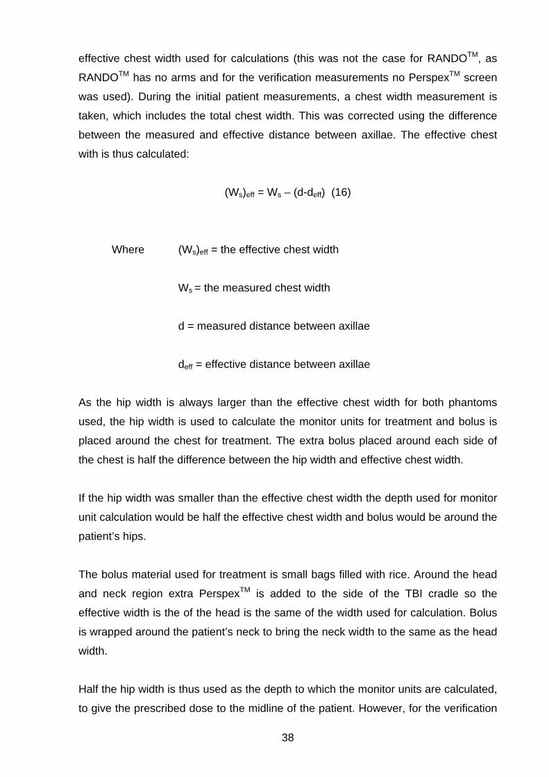
effective chest width used for calculations (this was not the case for RANDOTM, as
RANDOTM has no arms and for the verification measurements no PerspexTM screen
was used). During the initial patient measurements, a chest width measurement is
taken, which includes the total chest width. This was corrected using the difference
between the measured and effective distance between axillae. The effective chest
with is thus calculated:
(Ws)eff = Ws – (d-deff) (16)
Where (Ws)eff = the effective chest width
Ws = the measured chest width
d = measured distance between axillae
deff = effective distance between axillae
As the hip width is always larger than the effective chest width for both phantoms
used, the hip width is used to calculate the monitor units for treatment and bolus is
placed around the chest for treatment. The extra bolus placed around each side of
the chest is half the difference between the hip width and effective chest width.
If the hip width was smaller than the effective chest width the depth used for monitor
unit calculation would be half the effective chest width and bolus would be around the
patient’s hips.
The bolus material used for treatment is small bags filled with rice. Around the head
and neck region extra PerspexTM is added to the side of the TBI cradle so the
effective width is the of the head is the same of the width used for calculation. Bolus
is wrapped around the patient’s neck to bring the neck width to the same as the head
width.
Half the hip width is thus used as the depth to which the monitor units are calculated,
to give the prescribed dose to the midline of the patient. However, for the verification
38

measurements, the effective chest width was used and no bolus was added as the
measurement were taken around the chest region.
The monitor units are calculated using the following formula:
100 (10)( / 2, ) ( , ) ( )
D PSFMUTMR P S AAF x y PSF S ISL
× ×=
× × × (17)
Where D = prescribed dose per fraction multiplied by the beam weighting for
each field
PSF(10) = phantom scatter factor for a 10 x 10 cm field size
TMR(P/2,S) = tissue maximum ratio for the depth (half hip width) and
equivalent square size S
AAF(x,y) = air area factor for collimator jaw setting (a collimator scatter
factor).
PSF(S) = phantom scatter factor for equivalent field size S
ISL – inverse square law correction for the extended SAD of 400 cm
The inverse square law is:
ISL = 22
400100100
⎟⎠⎞
⎜⎝⎛=⎟
⎠⎞
⎜⎝⎛
SAD (18)
Phantom Verification – TLDs
Using calculations completed on the unmodified RANDOTM phantom, a plan was
developed using RadplanTM to treat the phantom with TLDs so the dose per monitor
unit could be measured.
39

There were many reasons why TLDs were chosen as the detector for this
application. These included their small size, which enabled them to fit into slots within
the RANDOTM phantom. TLDs have no cables attached, reusable and cost effective
and have good long-term stability and negligible environmental (temperature,
pressure, humidity) factors.
For the TLD measurements, the number of monitor units to be delivered was based
on the effective chest width using the ratio from the homogeneous and
inhomogeneous monitor units from the RadplanTM planning system and rather than
using the hip width for calculating the monitor units and then adding bolus as would
be done for treatment, as the aim was to assess the effective chest width calculation.
The TLDs used were Harshaw TLD-100 chips, which are lithium fluoride chips doped
with impurities of magnesium and titanium. The chips have a physical size of 3.2 x
3.2 x 0.89 mm and a density of 2.64 g/cm3 and a Zeff of 8.2. The TLDs are always
handled with vacuum tweezers.
Prior to use, the TLD system was calibrated according to the Westmead Hospital
clinical protocol. A reader calibration factor (RCF) was generated using a special
calibration set of TLDs. The RCF factor is the ratio of response of the instrument in
nanocoloumbs to the actual radiation to which the calibration dosimeters were
exposed, i.e. converting the readings from nC to cGy.
The set of TLDs used was a set of clinical TBI TLDs, calibrated for 2 Gy exposures.
Each TLD set in the chip was given an individual element correction coefficient
(ECC). The ECC for each dosimeter corrects its response to produce a response
equal to the average of all the dosimeters, as not all chips can be manufactured with
the same TL efficiency.
The TLD chips were calibrated in a PerspexTM phantom with holes drilled in it for
TLDs and Farmer style ion chamber placement. Ion chamber readings are corrected
for temperature and pressure. Conditions for calibrations should be as close as
possible to the conditions for TLD measurement, including using beams with the
same beam quality as for measurement and approximately 2 Gy being delivered to
both treatment and calibration chips to reduce supralinearity effects.
40

Before calibration and exposure measurements, TLDs are pre-annealed for one hour
at 400°C and then for two hours at 100°C. This also removes residual TL signals and
establishes TLD sensitivity.
The TLDs are placed into slots within the RANDOTM phantom especially designed for
TLD chips. Chips were placed into three slots on midplane about the calculation point
used in the planning systems. Diagram 3.3 shows red crosses where the TLDs were
positioned. It should be noted that there is some uncertainty introduced as the
calculation point was in the middle of the slice whereas TLDs are to be positioned
towards the edge of the slice.
Diagram 3.3 – Placement of the TLDs at the red crosses.
The phantom was positioned on a special TBI treatment couch at an extended FAD
of 4 metres as planned. The phantom was treated according to the plan, rotating the
phantom after each beam. (The bunker is wider on one side of the gantry than the
other, so rather then rotating the gantry to deliver the bilateral beams, the patient bed
is rotated). The phantom was aligned using a special TBI laser that points down a
line that is 4 metres from the source. This laser line was aligned to the midline of the
phantom. This process was repeated three times for three sets of TLDs and the
results averaged.
41

Some of the set of TLDs were reserved and are now used for scaling purposes for
supralinearity correction. The scaling dose is based on an estimate of what the dose
to the TLDs in the phantom was. The scaling is done in the calibration phantom,
together with an ion chamber to measure absolute dose. The ion chamber reading
was corrected for air density and other factors such as polarity.
After irradiation, fading occurs in TLDs, particularly in peaks not used for dosimetry.
In order to hasten the fading process, TLDs are post annealed for 10 minutes at
100°C prior to being read.
The automatic Harshaw 5500 reader was used. The TLDs are read with an
acquisition set up of a temperature ramp of 15°C/s to a maximum of 300°C with an
acquisition time of 33 1/3 seconds.
The results from the reader are transferred as an ASCII file to a Microsoft Excel
worksheet with a macro developed using Visual Basic for Applications to use the
reading from the scaling TLDs and a supralinearity corrections formula (fitted to
measured supralinearity curve) to correct the measured TLDs.
Phantom Verification – Film
Radiographic film was used as a two dimensional dosimeter to verify the dose
distributions produced by the treatment planning systems and the differences from
changing to the extended SAD used for treatment. Radiochromic film could also have
been used, but radiographic film was more cost effective and available in larger
sheets.
A sheet of ready-packed Kodak EDR2 film (Eastman Kodak Company, Rochester,
New York) from the same batch as the films used for phantom verification was used
for calibration. It was exposed to varying amounts of radiation using a 6 MV beam
from a Varian 6Ex Clinac from 0.25 Gy to 4 Gy, as calculated using measured
treatment planning data. 5 cm of solid water was used for backscatter and 1.5 cm of
solid water was placed on top of the film. Each segment of radiation had a field size
of 5 x 5 cm. The film was positioned at an SAD of 100 cm.
42

One envelope of ready-packed Kodak EDR2 film was positioned between slices of
the anthropomorphic phantom close to the calculation point used by the treatment
planning systems. The phantom slices were clamped together and were positioned at
TBI treatment position (TBI extended SAD of 400 cm) and 1966 monitor units were
delivered bilaterally, as per calculations based on heterogeneity correction for the
RANDOTM phantom produced by PinnacleTM, based a prescription of 2 Gy per
fraction. The film was removed and another film positioned and the phantom
repositioned so that the SAD was 100 cm. 123 monitor units were delivered
bilaterally.
Pin pricks were made in one corner of each film to mark the orientation of the film
and to allow for air pockets to be squeezed out of the pre packaged film envelopes to
prevent hot spots developing.
The films were left overnight to stabilise its optical density response. The film
envelopes were opened in the darkroom and each film was processed in an AGFA
classic E.O.S. automatic film processor, dedicated to use for radiotherapy films. All
the films were processed sequentially in the same batch to reduce processor
variation.
Following being processed the films were digitised using a VXR-16 Dosimetry Pro 16
bit CCD film scanner (VIDAR Systems Corporation, Herndon Virginia) and the
images were saved in TIFF image format.
These tiff image files were then loaded into the DoseLab 3.05 software (Childress,
2003) for analysis. The software calculates the dose at a point as being proportional
to the optical density of the film.
The calibration film was used to convert optical density to dose. The films from the
100 cm and 400 cm SAD phantom verification measurements were then converted to
dose and isodoses were calculated for comparison with the isodose distributions
produced by the treatment planning systems.
43

Chapter Four – Results
CT to density calibration
Diagram 4.1 shows the calibration of Hounsfield unit (HU) to density used by
PinnacleTM and RadplanTM.
HU
0
0.5
1
1.5
2
-1500 -1000 -500 0 500 1000 1500
HU
Mas
s D
ensi
ty
PinnacleRadplan
Diagram 4.1 – the Hounsfield calibration for density used by the planning systems.
The PinnacleTM system uses CT numbers so these have been converted to
Hounsfield number for display.
Ratio Differences: RadplanTM and PinnacleTM
Table 4.1 shows the effective chest widths calculated using the ratio between
heterogeneous and homogenous monitor units from PinnacleTM and RadplanTM and
the difference between the two models. The systematic difference arises because
PinnacleTM includes the effects of changes to scatter due to the heterogeneity. If the
effective chest width is larger than the hip width, bolus is added around the hips so
the effective chest width and the hip width are the same.
44

PinnacleTM effective chest
width (cm)
RadplanTM effective chest
width (cm)
Difference
Wide Short 20.8 20.1 3.4%Narrow Tall 22.8 21.9 3.9%Largest Lung 20.7 20.1 2.9%Smallest Lung 22.7 21.9 3.5%RANDOTM 22.6 21.9 3.1%
Table 4.1 – The effective chest widths calculated using the ratios between
heterogeneity and homogeneity calculations from PinnacleTM and RadplanTM for
different phantoms.
Table 4.2 shows the dose per monitor unit calculated using the effective chest width
based on the ratio of homogeneous and inhomogeneous monitor units calculations
produced by the treatment planning system together with the average dose per
monitor unit as measured by TLDs. The standard deviation for the TLD
measurements was ±4%, so both the PinnacleTM and RadplanTM dose delivered per
monitor unit agree within one standard deviation with the measured dose per monitor
unit.
Calculation/measurement technique Dose (Gy) per monitor unit at 400 cm
SAD
RadplanTM 0.105
PinnacleTM 0.102
TLD 0.106
Table 4.2 – Dose (Gy) per monitor unit at the extended TBI SAD of 400 cm as
calculated using the ratios from RadplanTM and PinnacleTM and measured using
TLDs.
45

Film Dose Response
Diagram 4.2 shows the exposed film used to determine the dose response curve and
diagram 4.3 shows the dose response curve obtained from the film and used for film
to dose calibration.
Diagram 4.2 – the calibration film used to convert optical density to dose.
46

Optical Density to Dose Calibration
0
1
2
3
4
0 1 2 3 4 5
Dose (Gy)
Opt
ical
Den
sity
Diagram 4.3 – the calibration curve used to convert optical density to dose. Isodose Distributions
All diagrams are normalised so that 100% of the prescribed dose is at the calculation
point on central axis midline.
Diagram 4.4 shows the isodose distribution produced by PinnacleTM for the
RANDOTM phantom in the transverse plane containing the calculation point, marked
by the orange cross on the isodose map. Diagram 4.5 shows the same thing for
RadplanTM. Diagram 4.6 shows the measured isodose distribution from the Kodak
EDR2 film at an SAD of 100 cm in RANDOTM, showing at least a reasonable
qualitative agreement with diagrams 4.4 and 4.5. It can be seen that the measured
dose as in diagram 4.6 receives a slightly higher dose in the centre of the chest than
either system calculated and shows better agreement with the distribution calculated
by PinnacleTM.
Diagram 4.7 shows the measured isodose distribution from Kodak EDR2 film at an
SAD of 400 cm in RANDOTM and diagram 4.8 shows the calculated isodose
distribution at 400 cm SAD from PinnacleTM.
47

Diagram 4.4 – isodose distribution in the transverse plane at 100 cm SAD calculated
by PinnacleTM.
Diagram 4.5 – isodose distribution in the transverse plane at 100 cm SAD calculated
by RadplanTM
48

Diagram 4.6 – measured isodose distribution from film at and SAD of 100 cm in
RANDOTM.
3.1 cm
3.1 cm
Diagram 4.7 – measured isodose distribution from film at extended SAD of 400 cm
in RANDOTM.
49

Diagram 4.8 – RANDOTM PinnacleTM isodose distribution with heterogeneity
correction at 400 cm SAD.
Diagram 4.9 – RANDOTM PinnacleTM isodose distribution without heterogeneity
correction at 100 cm SAD.
50

Diagram 4.10 – RANDOTM RadPlanTM isodose distribution without heterogeneity
correction at 100 cm SAD.
51

Chapter five – Discussion TBI involves complex dosimetry but the dosimetry due to the large SAD, dose
uniformity and flatness over the large field, bolus requirements, extra scatter from the
bunker walls and floor and large field overshoot. There is also a lack of specialised
treatment planning systems for TBI planning at extended SAD.
TBI involves complex dosimetry due to the large SAD. This changes the angular
distribution and electron contamination of the beam, changing the dose uniformity
and flatness over the large field. TBI dosimetry is also complex due to bolus
requirements, extra scatter from the bunker walls and floor and large field overshoot.
There is also a lack of specialised treatment planning systems for TBI planning at
extended SAD.
In this project the effective chest width for treatment monitor unit calculations and
bolus requirements was calculated. This value varies between the 2D Bentley –
Milan algorithm with modified Batho heterogeneity corrections and the 3D
convolution method by less than 4%. The width of the lungs caused the greatest
variation. Changing the height and depth of the lungs produced less than 1%
variation.
Having determined the difference between RadplanTM and PinnacleTM does not
change significantly due to lung size, the phantom verification work was completed
using RANDOTM, as TLD slots were available to position the TLDs. One
disadvantage with the RANDOTM phantom is it doesn’t have arms, which would affect
the dose distributions delivered in a real patient, as the arms would provide additional
shielding to the lungs. Hence TLDs were placed in RANDOTM and the measurements
showed that the dose per monitor unit using an effective chest width for monitor unit
calculations using the ratio between heterogeneity and homogeneity calculations
from RadplanTM and PinnacleTM varied less than 4%. According to the AAPM TG53
report, the recommended accuracy required in calculations from a treatment planning
system for a 3D calculation with heterogeneities present should be within 5%. This
shows that either method of calculating the effective chest width could be used for
calculating the number of monitor units for TBI treatments.
52

Each method also provides some isodose display information, although PinnacleTM
can display this information on all transverse slices as well as sagittal and coronal
views.
The sagittal and coronal views show the small air gaps between phantom slices that
would not be present in a patient and that RadplanTM would not have included in its
calculations. These gaps would not have been perfectly reproduced during each TLD
verification measurement, but it is unlikely this would have much effect on the results,
especially since the results were averaged over three simulated treatments.
In order to compare the two treatment planning systems the CT calibration curves
had to be compared. For densities lower than water/tissue equivalent, RadplanTM and
PinnacleTM calibration of density to Hounsfield number was almost the same.
However, some discrepancies can be seen with higher density materials which may
create some small changes between the two treatment planning systems for
RANDOTM due to the presence of bone. However, the ratio results for RANDOTM are
consistent with the RANDO lung phantom. These differences are due to changes in
the CT scanner between commissioning RadplanTM and PinnacleTM, but were not
significant enough to change the calibration curve in RadplanTM.
Another difference between RadplanTM and PinnacleTM is that the beam data for
RadplanTM and PinnacleTM was collected at different times. Also, RadplanTM directly
uses the measured PDD and beam profile data to calculate the dose distribution
whereas PinnacleTM uses a PDD to determine the beam energy spectrum and uses
this to model the dose distribution. The same beam data is used for heterogeneity
and homogeneity plans, so the ratio would cancel some of the differences from
different beam data measurements or models.
For verification TLDs placed in three locations for each simulated treatment so the
results of each three chips for each simulation could be averaged together, as well as
over three simulations. However, as the chips covered a wider area and were not all
surrounded by the 100% isodose, the TLD readings may vary slightly from 100% of
dose/monitor unit. Another uncertainty inherent in the TLD positioning is that the
53

calculation point was in the middle of the slice but the TLDs were placed in slots at
the edge of the slice.
TLDs are not as accurate as ion chambers but have the advantage of being able to
be placed directly into the phantom and without concern over cable and stem
irradiation. An ion chamber was not used in this project for verification, as there was
nowhere to position it.
TLDs are relative dosimeters so the accuracy is determined by reproducibility. In this
work the reproducibility of the TLD absorbed dose measurements had a standard
deviation of 4%. This error included errors due to setup for TBI treatment, such as
phantom positioning and accelerator variation.
The TLDs were scaled with the scaling chips being exposed directly after the
simulated TBI treatments. This should have helped the reproducibility by cancelling
out TLD batch sensitivity changes, reader changes, oven changes and accelerator
output. The calibrations for ECC and RCF were also completed under similar
conditions to increase reproducibility.
Kodak EDR2 film was also used as a planar dosimeter for verification of the isodose
distributions produced by the treatment planning systems. A dose response curve
was generated to ensure the films were exposed to radiation in the linear region of
the dose response curve and to be used for optical density to dose calibration. Film
response to radiation is not the same across the entire film and this could result in up
to a 2% variation in the response of the film. (Williams and Thwaites, 1993) The film
was also slightly smaller than the RANDOTM phantom as can be seen in the phantom
verification films in diagrams 4.6 and 4.7.
Kodak EDR2 film has previously been shown to have variations of less than 2%
compared to ion chambers except for larger field sizes and greater depth (>15 cm)
where errors in the range of 3-5% were reported (Chetty, 2002). Thus, particularly
around the calculation point for TBI treatments, the dose accuracy for the film may be
lower. Film also has some angular dependence and when exposed parallel to the
beam, as in the calibration, rather than perpendicular to the beam, some over
response may be seen. (Suchowerska, 2001)
54

As expected, changing the height of the lungs makes no difference to the monitor
units calculated by RadplanTM for the midplane as RadplanTM is a 2D system. There
was also no significant difference in the ratios when changing the height of the lungs
in PinnacleTM. This is because the calculation point is out the range of the main
scattered radiation from the edges of the lungs. The width of the lung made a
difference for the heterogeneous calculations for both the 2D and 3D system.
Because no significant variation in the ratios was observed, all further work focussed
only the smallest lungs and largest lungs.
When the ratios are used to manually calculate the doses required to treat a patient
with the RANDOTM lung phantom dimensions, because the effective chest width
always remains smaller than the width of the hip, the monitor units for treatment
remain the same. However, the plate separation would be different and hence
different amounts of bolus material would be added to build up the chest to the plate
separation width. This means that for cases where the effective chest width is smaller
than the width of the hips for both methods of calculating the ratio for the effective
chest width (RadplanTM and PinnacleTM), the only part of the body that receives a
different dose would be the chest, due to the changes in bolus material added.
Isodose distributions from different planning methods and measurements can be
quantitatively compared. Various methods for quantitative analysis of isodose
distributions include dose differences or distance to agreement analysis, which
combines both dose differences and distance to agreement. However, the software
options available during this project did not allow quantitative analysis of isodose
maps, so the isodose distribution maps were only visually compared.
The isodose distributions on transverse plane around the calculation point are similar
between RadplanTM and PinnacleTM but show some differences, especially anterior
and posterior to the lungs, as the Bentley – Milan algorithm does not calculate
differences in scatter from heterogeneities.
It is observed that there are differences in the isodose distributions between
RadplanTM and PinnacleTM even for homogeneous cases. This shows differences
55

between the two calculation methods, such as RadplanTM not calculating the change
in scatter due to changes in patient contour.
When comparing the results between the smallest lungs and largest lungs in the
RANDOTM lung phantom the doses are higher around the calculation pt in the largest
lungs case. This effect is seen more in PinnacleTM, showing an increase in the scatter
component from the extra lung volume not calculated in RadplanTM. This is also why
it is the midplane dose is higher in heterogeneous cases than homogeneous cases.
During treatment of patients, patient positioning changes, involuntary and voluntary
patient motion (including breathing with changes to lung volume), changes to patient
size and bolus distribution between fractions add to the potential errors of TBI
treatment. Hence invivo dosimetry is critical during TBI treatments.
In the future it is possible that computer improvements, such as treatment planning
computers being able to accept larger CT imaging data sets and having increased
computation speeds, will aid 3D planning for TBI. The difference in measured
isodose distributions between 100 and 400 cm SAD also suggests that using beam
data from an extended SAD would be a future improvement so isodoses and DVHs
can be more accurately used for dose evaluation if required during TBI.
56

Chapter Six – Conclusion
This project compared two planning methods for calculating the heterogeneity
correction required for determining the effective chest width for planning TBI, taking
into account possible effects of different lung sizes. The two planning methods were
the 2D Bentley – Milan algorithm with modified Batho heterogeneity corrections and
3D convolution planning methods. Measurements were made in an anthropomorphic
phantom with films and TLDs to verify the results.
An anthropomorphic phantom was modified with different lung size inserts and four
different lung sizes were calculated on both treatment planning systems. The process
was repeated using the unmodified anthropomorphic phantom, which had slots for
TLD measurements for verification measurements.
For an isocentric treatment, the treatment planning system for each lung size
calculated the monitor units required to deliver the prescribed dose to the midline for
both with and without heterogeneity corrections.
The ratio between the number of monitor units required with and without
heterogeneity corrections was used to calculate the effective chest width of the
patient. This was compared to the measured hip width and the larger value was used
to calculate the monitor units required to deliver the prescribed dose to the midline at
TBI treatment SAD. The effective chest width varied less than 4%.
The effect of different lung sizes was only seen where the width of the lungs
changed. Changes to the height or depth of the lungs had no significant effect on the
calculations of the effective chest width, as was to be expected as changing the
height and depth of the lungs only changes the scatter component.
The isodose distributions in the transverse plane were also measured with Kodak
EDR2 film and showed reasonable agreement between the calculated and measured
isodoses at isocentre. The isodose distribution changed significantly at the extended
TBI treatment SAD of 400 cm. However, the changes showed a more uniform dose
distribution at the extended SAD, as expected.
57

The dose per monitor unit at treatment SSD was then calculated for the TBI
treatment SSD without any bolus or tissue compensation based on the effective
chest width from both planning systems and this was compared to a dose per
monitor unit value measured in RANDOTM using TLDs.
Whilst the heterogeneity corrections were different between the planning systems,
The difference was smaller than one standard deviation of measurements from the
TLDs, so no significant difference could be detected between each planning method
and the TLD measurements, which had an accuracy of 4%. This is within the 5%
accuracy required. The isodose distributions produced by both treatment planning
systems showed reasonable agreement with the isodose measurements taken at
isocentre. This shows that either method of planning TBI would be suitable for clinical
purposes.
58

References
1. Harden SV, Routsis DS, Geater AR et al. Total body irradiation using a
modified standing technique: a single institution 7 year experience. BJR 74:
1041 – 1047, 2001
2. Cosset JM, Socie G, Dubray B et al. Single dose versus fractionated total
body irradiation before bone marrow transplantation: radiobiological and
clinical considerations. Int J Radiat Oncol Biol Phys. Sep;30(2):477-92, 1994
3. Shank B, Chu FC, Dinsmore R et al. Hyperfractionated total body irradiation
for bone marrow transplantation. Results in 70 leukemia patients with
allogenic transplants. Int J Radiat Oncol Biol Phys. Nov;9(11):1607-11, 1983
4. International commission on Radiation Units and Measurements. Prescribing,
recording and reporting photon beam therapy. Report 50. Bethesda, MD:
ICRU, 1993.
5. Sanchez-Doblano F. Quast U, Arrans R et al. Reporting total body irradiation
prior to bone marrow transplantation. ISBN: 84-605-3132-5, EBMT, Sevilla,
1995
6. Vollans SE, Perrin B, Wilkinson JM et al. Investigation of dose homogeneity in
paediatric anthropomorphic phantoms for a simple total body irradiation
technique. BJR Br J Radiol. Mar;73(867):317-21, 2000
7. Sanchez-Nieto B, Sanchez-Doblano F, Terron JA. A CT-aided PC based
physical treatment planning of TBI: A method for dose calculation. Radiother
and Oncol. 42:77-85, 1997
8. Abraham D et al. TBI treatment planning using the ADAC Pinnacle Treatment
planning system. Med Dosim. 25(4):219-224, 2000
9. Smith CL, Chu WK, Goede MR et al. An analysis of the elements essential in
the development of a customised TBI program. Med Dosim. 21(2):49-60, 1996
59

10. Sanchez-Nieto B, Sanchez-Doblano F, Arrans R et al. Backscatter correction
algorithm for TBI treatment conditions. Med Dosim. 18:107-111, 1993
11. Curran WJ, Galvin JM, D’Angio GJ. A simple dose calculation method for total
body photon irradiation. IJROBP 17:219-24, 1989
12. AAPM Report 17. The physical aspects of total and half body photon
irradiation. Editors: Van dyk J, Galvin JM, Glasgow GP, Podgorsak EB. Task
Group 20 of the Radiation Therapy Committee of the American Association of
Physicists in Medicine, 1986.
13. Rider WD, Van Dyk J. Total and partial body irradiation. In: Radiation therapy
Treatment Planning.. Editors: Bleehan NM, Glatstein E, Haybittle JL. Marcel
Dekker, New York, 559-594, 1983.
14. Van Dyk J. Dosimetry for total body irradiation. Radiother Oncol. 9:107-118,
1987.
15. Mayneord WV, Lamerton LF. A survey of depth dose data. BJR 14:255, 1944
16. Doughty D, Lambert GD, Hirst A et al. Improved total-body irradiation
dosimetry. BJR 60;269-78, 1987.
17. Fiorino C, Mangili P, Cattaneo GM et al. Polarity effects of ionisation chambers
used in TBI dosimetry due to cable irradiation.
18. De Sapio E et al. Optimization of a dosimetric procedure in total body
irradiation. Radiol Med Torino Jun;79(6):624-7, 1990.
19. Quast U. Physical problems of total body irradiation. Strahlenther Onkol. 1986
Apr;162(4):233-6.
20. Khan FM. The Physics of Radiation Therapy. 2nd Ed. Baltimore: Williams and
Wilkins; 2003.
60

21. Obcemea CH, Rice RK, Mijnheer BJ et al. Three-dimensional dose distribution
of total body irradiation by a dual source total body irradiator. IJROBP 24:789-
793, 1992
22. Amor Duch M, Ginjaume M, Chakkor H et al. Thermoluminescence dosimetry
applied to in vivo dose measurements for total body irradiation techniques.
Radiother Oncol. 47:319- 324, 1998
23. Khan FM, Williamson JF, Sewchand W et al. Basic data for dosage calculation
and compensation. IJROBP 6:745-751 (1980)
24. Svahn-Tapper G, Nilsson P, Jönsson C et al. Calculation and measurements
of absorbed dose in total body irradiation. Acta Oncol 29 (1990)
25. ICRU 21. Radiation Dosimetry: Electrons with initial energies between 1 and
50MeV. International Commission on Radiation units and Measurements.
Report No 21, Washington DC, USA 1972.
26. Syh HW, Chu WK, Kumar P et al. Estimation of the mean effective organ
doses for total body irradiation from RANDO phantom measurements. Med
Dosim. 17:103-106, 1992.
27. Kirby TH, Hanson WF, Cates DA. Verification of total body photon irradiation
dosimetry techniques. Med Phys. 15(3): 364-369, 1988
28. Podgorsak EB, Pla C, Evans, DC et al. The influence of phantom size on
output, peak scatter factor, and percentage depth dose in large-field photon
irradiation. Med Phys 12(5): 639-645, 1985
29. Yuille PG, Wielinga W, Crestani EA. Fractionated total body irradiation in
bone marrow transplantation – an emphasis on lung dosimetry. Australas
Radiol 27: 186-194, 1983.
61

30. Metcalfe P, Kron T, Hoban P. The physics of radiotherapy x-rays from linear
accelerators. Medical Physics Publishing. 1997
31. Quast U. Dosimetry of Total Body Irradiation – A review. Dosimetry in
Radiotherapy Vol 2, Proceedings of a symposium Vienna, 31 August – 4
September 1987 IAEA
32. International commission on Radiation Units and Measurements. Dose
Specification for Reporting External Beam Therapy with Photons and
Electrons. Report 29. ICRU, 1978.
33. El-Khatib E, Battista JJ. Accuracy of lung dose calculations for large-field
irradiation with 6-MV x rays. Med Phys 13(1): 111-116, 1986
34. Lulu BA, Bjarngard BE. Batho’s correction factor combined with scatter
summation. Med Phys 9(3): 372-7, 1982
35. Butson MJ, Elferink R, Cheung T et al. Verification of lung dose in an
anthropomorphic phantom calculated by the collapsed cone convolution
method. Phys Med Biol 45 (11): N143 –149, 2000
36. Batho HF. Lung corrections in Cobalt 60 beam therapy. J. Can. Assoc. Radiol.
15: 79 – 83, 1964
37. Sontag MR, Cunningham JR. Corrections to absorbed dose calculations for
tissue inhomogeneities. Med Phys 18(4):719 – 723, 1991
38. Webb S, Fox RA. The direct use of CT data for inhomogeneity corrections in
radiotherapy planning. Br. J. Radiol. Suppl 15, 1979
39. International commission on Radiation Units and Measurements. Tissue
substitutes in radiation dosimetry and measurement. Report 44. ICRU, 1989
40. The Merck Manual of Diagnosis and Therapy. 17th Edition. Edited by Beers
MH and Berkow R. 1999-2005, Merck & Co.
62

41. Bomford CK and Kunkler IH. Walter and Miller’s Textbook of Radiotherapy. 6th
Ed. Elsevier Science Limited. 2003
42. Williams JR and Thwaites DI. Radiotherapy physics in practice. Oxford
University Press. 1993
43. IAEA TRS 398. Absorbed dose determination in external beam radiotherapy:
an international code of practice for dosimetry based on standards of
absorbed dose to water. International Atomic Energy Agency. 2000
44. AAPM TG53. Quality assurance for clinical radiotherapy treatment planning.
Editors: Fraass B, Doppke K et al. Task Group 53 of the Radiation Therapy
Committee of the American Association of Physicists in Medicine, 1998.
45. International commission on Radiation Units and Measurements.
Determination of absorbed dose in a patient irradiated with beams of X or
gamma rays in radiotherapy procedures. Report 24. ICRU, 1976
46. Chilress NL, Salehpour M, Dong L et al. Dosimetric accuracy of Kodak EDR2
film for IMRT verifications. Med Phys 32(2): 539-48, 2005
47. Bucciolini M, Buonamici FB, Casati M. Verification of IMRT fields by ilm
dosimetry. Med Phys 31:161-168, 2004
48. Childress NL, Rosen II. Effect of processing time delay on the dose response
of Kodak EDR2 film. Med Phys 31(8):2284-8, 2004
49. Dogan N, Leybovich LB, Sethi A. Comparative evaluation of Kodak EDR2 and
XV2 films for verification of intensity modulated radiation therapy. Phys med
Biol 47(20):3629-3641, 2002
50. Ekstrand K, Greven K, WU K. The influence of x-ray energy on lung dose
uniformity in total-body irradiation. Int J Rad Biol Phys Jul 38(5):1131-6, 1997
63

51. Chetty IJ, Charland PM. Investigation of Kodak extended dose range (EDR)
film for megavoltage photon beam dosimetry. Phys Med Biol 47(22):4121-30,
2002
52. Childress NL, Rosen I. DoseLab 3.05 – An open source dose comparison
software package for medical physicists. Nov 2003
53. Thomas ED. Total body irradiation regimens for marrow grafting. Int J Rad Biol
Phys 19:1285-8, 1990
54. Galvin JM, D’Angio GJ, Walsh G. Use of tissue compensators to improve the
dose uniformity for total body irradiation. Int J Rad Biol Phys 6:767-771, 1980
55. Kim TH, Khan FM, Galvin JM. A report of the work party: comparison of total
body irradiation techniques for bone marrow transplantation. Int J Rad Biol
Phys 6:779-784, 1980
56. ICRP Publication No. 44. Protection of the patient in radiation therapy. Annals
of the ICRP 15(2), 1985
57. Milan J, Bentley RE. The storage and manipulation of radiation dose data in a
small digital computer. Br J Radiol. 47(554):115-21, 1974
58. Storchi P, Woudstra E. Calculation of the absorbed dose distribution due to
irregularly shaped photon beams using pencil beam kernels derived from
basic beam data. Phys Med Biol, 41(4):637-56, 1996
59. Johns HE, Cunningham JR. The Physics of Radiology. 4th Ed. Charles C
Thomas Publisher. 1983
60. IEC 61217 Radiotherapy Equipnment – Coordinates, Movements and Scales
(Consolidated edition), 2002.
61. Suchowerska N, Hoban P, Butson M et al. Directional dependence in film
dosimetry: radiographic and radiochromic film. Phys Med Biol, 46 (5):1391 –
1397, 2001
64

65