Embed Size (px)
Citation preview
This content has been downloaded from IOPscience. Please scroll down to see the full text.
Download details:
IP Address: 218.104.71.166
This content was downloaded on 08/05/2015 at 02:16
Please note that terms and conditions apply.
Comparison of the transport properties of two-temperature argon plasmas calculated using
different methods
View the table of contents for this issue, or go to the journal homepage for more
2015 Plasma Sources Sci. Technol. 24 035011
(http://iopscience.iop.org/0963-0252/24/3/035011)
Home Search Collections Journals About Contact us My IOPscience

1 © 2015 IOP Publishing Ltd Printed in the UK
X N Zhang1, H P Li2, A B Murphy3 and W D Xia1
1 Department of Thermal Science and Energy Engineering, University of Science and Technology of China, Hefei, Anhui Province 230026, People’s Republic of China2 Department of Engineering Physics, Tsinghua University, Beijing 100084, People’s Republic of China3 CSIRO Manufacturing Flagship, PO Box 218, Lindfield NSW 2070, Australia
E-mail: [email protected] and [email protected]
Received 26 February 2015, revised 29 March 2015Accepted for publication 7 April 2015Published 7 May 2015
AbstractTwo main methods have been used to calculate the transport properties of two-temperature (2-T) plasmas in local chemical equilibrium: the method of Devoto (method B), in which coupling between electrons and heavy species is neglected, and the method of Rat et al (method C), in which coupling is included at the cost of a considerable increase in complexity. A new method (method A) has recently been developed, based on the modified Chapman–Enskog solution of the species Boltzmann equations. This method retains coupling between electrons and heavy species by including the electron–heavy-species collision term in the heavy-species Boltzmann equation. In this paper, the properties of 2-T argon plasmas calculated using the three methods are compared. The viscosity, electrical conductivity and translational thermal conductivity obtained using all three methods are very similar. method B does not allow a complete set of species diffusion coefficient to be obtained. It is shown that such a set can be calculated using method A without any significant loss of accuracy. Finally, it is important to note that, by using the physical fact that the mass of heavy particles is much larger than that of electrons (i.e. me << mh), the complexity of calculations using method A is not increased compared with method B; that is to say, the calculation procedure is much simpler than with method C.
Keywords: two-temperature plasma, transport coefficients, Chapman–Enskog method, argon plasma
S Online supplementary data available from stacks.iop.org/PSST/24/035011/mmedia
(Some figures may appear in colour only in the online journal)
1. Introduction
The Chapman–Enskog method [1, 2] has been successfully used for many decades to calculate the transport properties for thermal plasmas in local thermodynamic equilibrium (LTE). The distribution function for different species is assumed to be Maxwellian with a first-order perturbation function, which is expanded in a finite series of Sonine polynomials. This linear-izes the Boltzmann equation and leads to the introduction of a system of linear equations. The final results of the linear equa-tions, i.e. the transport coefficients, are expressed as functions
of bracket integrals, which are dependent upon the interaction potentials characterizing different collision processes. Based on this method, many results for the commonly used pure gas and gas mixture plasmas in LTE have been published (e.g. [3–9] and papers cited therein). However, with the development of plasma diagnostics, it has become increasingly clear that the assump-tion that the LTE exists in thermal plasmas is often invalid. For example, deviations from LTE inevitably occur in the fringes of plasmas under interactions with the surrounding cold gas, in the regions where the plasma interacts with the workpiece, or in the vicinity of cold electrode walls [10–12]. A two-temperature
Plasma Sources Science and Technology
Comparison of the transport properties of two-temperature argon plasmas calculated using different methods
X N Zhang et al
Printed in the UK
035011
Psst
© 2015 IOP Publishing Ltd
2015
24
Plasma sources sci. technol.
Psst
0963-0252
10.1088/0963-0252/24/3/035011
Papers
3
Plasma sources science and technology
IOP
0963-0252/15/035011+17$33.00
doi:10.1088/0963-0252/24/3/035011Plasma Sources Sci. Technol. 24 (2015) 035011 (17pp)

X N Zhang et al
2
(2-T) plasma model is widely used to describe non-LTE plasmas under the assumption of local chemical equilibrium (LCE). In such plasmas, the temperature of electrons (Te) is higher than that of heavy species (Th), while the population densities of dif-ferent excited states of the heavy species satisfy the Boltzmann distribution with the characteristic temperature Tex = Te, where Tex is the excitation temperature.
Accurate evaluation of the transport properties of 2-T plasmas is one of the prerequisites for predicting the char-acteristics of thermal plasmas. To calculate the 2-T plasma transport coefficients, the decoupled method was first intro-duced by Devoto in 1965 [13], and was later modified, with a redefinition of the diffusion driving force, by Bonnefoi [14]. In Devoto’s decoupled method, the Boltzmann equa-tions for electrons and heavy species are solved separately by neglecting the electron–heavy-species collision term and the diffusion process between electrons and heavy species. This method significantly simplifies the calculation, and has been widely and successfully applied to LTE plasmas. However, the diffusion coefficients obtained by this decoupled theory do not satisfy the mass conservation law in the plasma system for the case of a 2-T plasma [15]. In order to solve this problem, Rat et al [16] proposed a fully coupled method, maintaining the coupling between electrons and heavy species without any simplifications. However, due to the complexity of the cal-culation, and the negligible differences between the results obtained for transport coefficients (other than the diffusion coefficients) and those obtained using Devoto’s decoupled method, Rat’s coupled method is rarely adopted to calculate the transport coefficients for 2-T plasmas. More recently, a new simplified method was derived by Zhang et al [17]. The coupling between electrons and heavy species is taken into account, but reasonable assumptions based on the physical fact that me << mh are adopted to allow some simplifications in solving the Boltzmann equations for electrons and heavy species. Zhang et al predicted that, using this new simplified method, it would be possible to obtain a complete and accu-rate set of diffusion coefficients, with a much simpler calcula-tion than that of Rat’s coupled theory.
In this paper, this simplified method is applied for the first time, to the case of an atmospheric-pressure 2-T argon plasma for electron temperatures from 300 to 30 000 K, which corre-sponds to the range of interest for most thermal plasmas [18]. Four species are taken into account in this calculation, i.e. argon atoms (Ar), singly ionized argon ions (Ar+), doubly ion-ized argon ions (Ar2+) and electrons (e). A detailed comparison between the calculated transport coefficients and those obtained using Devoto’s decoupled theory and Rat’s coupled theory is presented. The influence of the electron–heavy-species colli-sion term on the transport coefficients is also discussed.
The methods used to calculate the compositions and colli-sion integrals for 2-T argon plasma are presented in the sec-tion 2. The results obtained using the three different methods (Devoto’s method [13], Rat’s method [16] and the method pro-posed by Zhang et al [17]) are compared in section 3, and the effects of electron–heavy-species collision term on the diffu-sion coefficients are discussed. Major conclusions are presented in section 4. Appendix A gives the detailed differences between
the three methods mentioned above. Finally, the results of trans-port coefficients for 2-T argon plasma calculated by using the new method are tabulated in appendix B.
2. Plasma compositions and collision integrals
The composition of the plasma is one of the prerequisites for the calculation of its transport coefficients. In LTE, the equilibrium composition of the plasma can be determined by using the minimization of Gibbs free energy or the Saha equation. However, the choice of the appropriate method to calculate the composition of multi-temperature plasma is still controversial. Different forms of the multi-temperature Saha equation have been derived by different authors [19–22]. It has been pointed out by Giordano and Capitelli [23, 24] that the different forms of the Saha equation originate from the use of different thermodynamic constraints, i.e. the minimi-zation of internal energy (Gibbs or Helmholtz free energy, depending on the variables used) and the maximization of entropy. Chen and Han [20] argued that the minimization of Gibbs or Helmholtz free energy could not be used without corrections in 2-T plasmas, and the derivations based on the maximization of entropy were correct. In contrast, Andre et al [25] argued that the principle of entropy maximization is invalid in 2-T plasmas, since no conclusions about the time evolutions of the entropy can be drawn from the viewpoint of statistical mechanics.
In this work, for 2-T argon plasmas in LCE, we have used the Saha equations presented by Chen and Han [20], together with Dalton’s law and the charge neutrality conditions, which are given by
⎜ ⎟⎛⎝
⎞⎠
⎛⎝⎜
⎞⎠⎟π= ⋅ ⋅n n
n
m k T
h
Q T
Q T
E
k T2
2 ( )
( )exp ,i
a
i
a
ie e B e2
32 int
eint
e B e
(1)
= ⋅ ⋅⎜ ⎟⎛⎝
⎞⎠
⎛⎝⎜
⎞⎠⎟n n
n
πm k T
h
Q T
Q T
E
k T2
2 ( )
( )exp ,d
i
d
i
de e B e2
32 int
e
inte B e
(2)
∑= +=
p n k T n k T ,j
N
je B e
2
B h (3)
∑ ==
n Z 0,j
N
j j
1
(4)
where nj is the number density of species j, the subscripts ‘a’, ‘i’ and ‘d’ represent atoms, singly ionized ions and doubly ion-ized ions, while Zj is the value of charge number of species j, and kB and h are the Boltzmann constant and Planck constant. Ej is the ionization energy, calculated taking into account the lowering of the ionization potential [26]. The internal partition function, Q T( ),j
inte were evaluated from the energy levels of the
electronic states of species j tabulated by Moore [27], except those above the lowered ionization potential.
The calculated species number densities of the 2-T argon plasmas as the functions of the electron temperature (Te) and
Plasma Sources Sci. Technol. 24 (2015) 035011
X N Zhang et al
3
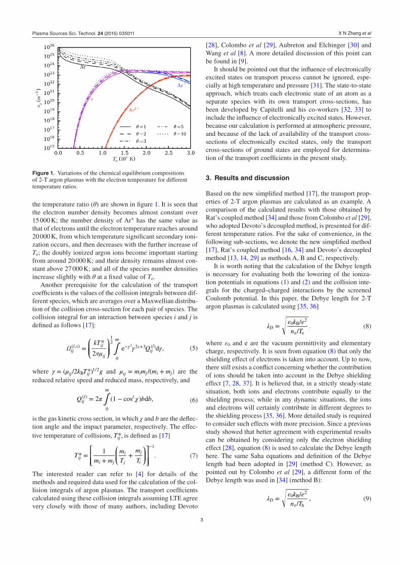
the temperature ratio (θ) are shown in figure 1. It is seen that the electron number density becomes almost constant over 15 000 K; the number density of Ar+ has the same value as that of electrons until the electron temperature reaches around 20 000 K, from which temperature significant secondary ioni-zation occurs, and then decreases with the further increase of Te; the doubly ionized argon ions become important starting from around 20 000 K; and their density remains almost con-stant above 27 000 K; and all of the species number densities increase slightly with θ at a fixed value of Te.
Another prerequisite for the calculation of the transport coefficients is the values of the collision integrals between dif-ferent species, which are averages over a Maxwellian distribu-tion of the collision cross-section for each pair of species. The collision integral for an interaction between species i and j is defined as follows [17]:
∫ γ γ= γ∞
− +⎛
⎝⎜⎜
⎞
⎠⎟⎟Ω
kT
πμQ
*
2e d ,ij
l s ij
ij
sijl( , )
12
0
2 3 ( )2 (5)
where γ μ= k T g( /2 *)ij ijB1/2 and μ = +m m m m/( )ij i j i j are the
reduced relative speed and reduced mass, respectively, and
∫π χ= −∞
Q b b2 (1 cos ) d ,ijl l( )
0
(6)
is the gas kinetic cross section, in which χ and b are the deflec-tion angle and the impact parameter, respectively. The effec-tive temperature of collisions, T*,ij is defined as [17]
⎡
⎣⎢⎢
⎛
⎝⎜
⎞
⎠⎟⎤
⎦⎥⎥
=+
+−
Tm m
m
T
m
T*
1.ij
i j
i
j
j
i
1
(7)
The interested reader can refer to [4] for details of the methods and required data used for the calculation of the col-lision integrals of argon plasmas. The transport coefficients calculated using these collision integrals assuming LTE agree very closely with those of many authors, including Devoto
[28], Colombo et al [29], Aubreton and Elchinger [30] and Wang et al [8]. A more detailed discussion of this point can be found in [9].
It should be pointed out that the influence of electronically excited states on transport process cannot be ignored, espe-cially at high temperature and pressure [31]. The state-to-state approach, which treats each electronic state of an atom as a separate species with its own transport cross-sections, has been developed by Capitelli and his co-workers [32, 33] to include the influence of electronically excited states. However, because our calculation is performed at atmospheric pressure, and because of the lack of availability of the transport cross-sections of electronically excited states, only the transport cross-sections of ground states are employed for determina-tion of the transport coefficients in the present study.
3. Results and discussion
Based on the new simplified method [17], the transport prop-erties of 2-T argon plasmas are calculated as an example. A comparison of the calculated results with those obtained by Rat’s coupled method [34] and those from Colombo et al [29], who adopted Devoto’s decoupled method, is presented for dif-ferent temperature ratios. For the sake of convenience, in the following sub-sections, we denote the new simplified method [17], Rat’s coupled method [16, 34] and Devoto’s decoupled method [13, 14, 29] as methods A, B and C, respectively.
It is worth noting that the calculation of the Debye length is necessary for evaluating both the lowering of the ioniza-tion potentials in equations (1) and (2) and the collision inte-grals for the charged–charged interactions by the screened Coulomb potential. In this paper, the Debye length for 2-T argon plasmas is calculated using [35, 36]
λ ε= k e
n T
/
/.D
0 B2
e e (8)
where ε0 and e are the vacuum permittivity and elementary charge, respectively. It is seen from equation (8) that only the shielding effect of electrons is taken into account. Up to now, there still exists a conflict concerning whether the contribution of ions should be taken into account in the Debye shielding effect [7, 28, 37]. It is believed that, in a strictly steady-state situation, both ions and electrons contribute equally to the shielding process; while in any dynamic situations, the ions and electrons will certainly contribute in different degrees to the shielding process [35, 36]. More detailed study is required to consider such effects with more precision. Since a previous study showed that better agreement with experimental results can be obtained by considering only the electron shielding effect [28], equation (8) is used to calculate the Debye length here. The same Saha equations and definition of the Debye length had been adopted in [29] (method C). However, as pointed out by Colombo et al [29], a different form of the Debye length was used in [34] (method B):
λ ε= k e
n T
/
/,D
0 B2
e h (9)
Figure 1. Variations of the chemical equilibrium compositions of 2-T argon plasmas with the electron temperature for different temperature ratios.
Plasma Sources Sci. Technol. 24 (2015) 035011

X N Zhang et al
4
along with the different forms of the Saha equations:
θ= ⋅ ⋅⎜ ⎟⎛⎝
⎞⎠
⎛⎝⎜
⎞⎠⎟n n
n
πm k T
h
Q T
Q T
E
k T2
2 ( )
( )exp ,i
a
i
a
ie e B e2
32 int
eint
e B e
(10)
θ= ⋅ ⋅⎜ ⎟⎛⎝
⎞⎠
⎛⎝⎜
⎞⎠⎟n n
n
πm k T
h
Q T
Q T
E
k T2
2 ( )
( )exp .d
i
d
i
de e B e2
32 int
e
inte B e
(11)
Through affecting the chemical equilibrium compositions of the 2-T plasmas, the different Saha equations can lead to dif-ferent values of the transport coefficients.
The different sets of Saha equations and different defini-tions of the Debye length that were used by Rat et al [34] and Colombo et al [29] influence the values of the transport coef-ficients that they presented. This makes comparison of the results we calculated using method A with those calculated using methods B and C more difficult. Our approach will be to compare our results with those presented by Rat et al and Colombo et al and to comment on the reasons for the differ-ence. We have also performed our own calculations using the Saha equations and Debye length adopted by Rat et al, so we are able to state whether the differences are due to different sets of Saha equations, different definitions of the Debye length, or fundamental differences between methods A, B and C.
We take the electrical conductivity (σ) as an example to reveal the influence of the different sets of Saha equations and different definitions of the Debye length. The electrical con-ductivity calculated using the different forms of Saha equa-tions and different definitions of Debye length is shown in figure 2. It is seen in figure 2(a) that: (i) under LTE (θ = 1), the results are exactly the same since equations (10) and (11) reduce to their counterparts equations (1) and (2), respectively; (ii) the values of σ calculated with the Saha equations (10) and (11) used in method B are higher than those obtained with the equations (1) and (2) used in this work at low electron tempera-tures; for example, the relative discrepancies between the cal-culated electrical conductivities using these two different sets of Saha equations are about 10.6% for θ = 2 and about 18.5% for θ = 3 for the case of Te = 12 000 K; (iii) in the high elec-tron temperature range (over around 20 000 K), use of the Saha equations (10) and (11) leads to much lower values of σ than those obtained using equations (1) and (2). The results shown in figure 2(b) indicate that the electrical conductivity is very sen-sitive to the definition of the Debye length. Except for the case of LTE plasmas, for which σ is the same due to the consistency of equations (8) and (9) with θ = 1, the electrical conductivi-ties calculated using equation (9) are much higher than those obtained using equation (8). This is because that the different definitions of the Debye length result in different values of the collision integrals for interactions between charged species [37]; the electrical conductivity is, to a good approximation,
proportional to the value of ∑ ≠( )n T n Ω .j j je e e e(1,1) The effect
of both the Saha equations and the Debye length on the calcu-lated electrical conductivity is presented in figure 2(c), which shows an almost linear superposition of the contributions from different Saha equations and different definitions of the Debye length.
3.1 . Comparison of the calculated transport coefficients using the different methods
In this section, the transport coefficients are calculated with θ = 1, 2, 3, 5 and 10, among which the data corresponding to θ = 1, 2 and 3 are used for comparison with the data presented in [34] (method B) and [29] (method C).
Figure 2. Comparisons of the electrical conductivity calculated: (a) using different Saha equations (line: equations (1) and (2); symbols: equations (10) and (11)); (b) using different definitions of the Debye length (line: equation (8); symbols: equation (9)); (c) combined effect of different Saha equations and definitions of the Debye length (line: equations (1), (2) and (8); symbols: equations (9)–(11)).
Plasma Sources Sci. Technol. 24 (2015) 035011

X N Zhang et al
5
Based on the preceding analysis, the calculated electrical conductivities for argon plasmas using methods A, B and C are compared in figure 3. The common features for the elec-trical conductivities calculated using different methods are: (i) for a fixed value of θ, the electrical conductivity increases with electron temperature due to the increase in the electron number density; (ii) there exists a further increase of the elec-trical conductivity above the electron temperature of around 26 000 K arising from the contribution of the secondary ioni-zation process; (iii) the thermal non-equilibrium degree (θ) affects the electrical conductivity through its influence on the electron number density (figure 1). The differences shown in figure 3(a) are as follows: in the high temperature range, above 20 000 K, method C somewhat overestimates the elec-trical conductivity compared with method A both in and out of LTE state, due to the use of different methods. This differ-ence can reach, for example, about 2.8% for θ = 2 at 22 000 K. As discussed in section 3.1, there exists a large difference between the calculated values of σ using method A and B, and this difference results from the usage of different Saha equa-tions and Debye length definitions rather than the different methods for calculating the electrical conductivity itself. This is verified by our further numerical experiment, the results of
which are shown in figure 3(b), where exactly the same results are obtained if the same formulas for calculating the plasma compositions and the Debye length (equations (9)–(11)) are used in method A and B.
The calculated viscosity is shown in figure 4. It is seen that the viscosity increases with temperature up to around 10 000 K, at which a significant level ionization occurs both in and out of LTE. As temperature increases further, the viscosity decreases rapidly as the long range Coulomb force between charged particles becomes important, because the viscosity is, to a good approximation, proportional to a weighted average
of −Ω[ ]ij(2,2) 1 at a given temperature [4]. At a fixed electron tem-
perature, the viscosity decreases with increasing temperature ratio (θ), since the value of Th is reduced with increasing θ at a given value of Te. Because the viscosity is primarily a prop-erty of the heavy species, and is barely influenced by the col-lisions between electrons and heavy species that are neglected in method C, the viscosities calculated using method A and C are consistent with each other. There do exist differences between the calculated results using method A and B for the non-equilibrium cases, especially in the electron temperature range between 10 000 and 20 000 K. Our calculation shows that these differences are mainly due to the different methods used for the calculation of the plasma compositions, since the influence of different choices of the Debye length on the vis-cosity are negligible. If the same method is used to evaluate the chemical compositions of the plasmas, then the discrepan-cies disappear.
In the new simplified theory, the energy flux of electrons caused by heat conduction can be written as [17]
θ= − ∇ − ∇θ q k T k T ln ,e e h e e (12)
where ke is the electron translational thermal conductivity, and θke is the electron non-equilibrium thermal conductivity, which
is introduced based on the assumption of equation (A.10). It can be seen that the electron translational thermal conduc-tivity is defined with respect to the gradient of the heavy-species temperature (Th). In order to be consistent with the traditional definition of the thermal conductivity and to allow
Figure 3. (a) Comparison of the electrical conductivity calculated using methods A, B ([34]) and C ([29]), and (b) verification on the influences of different Saha equations and different definitions of Debye length for methods A and B.
Figure 4. Comparison of the viscosity calculated using methods A, B ([34]) and C ([29]).
Plasma Sources Sci. Technol. 24 (2015) 035011
X N Zhang et al
6
for the comparison with the results obtained using the other two methods, the energy flux of electrons is rewritten as
λ λ θ= − ∇ − ∇θ q T ,e e e e (13)
where
λ θ λ θ= = −θ θk k k T/ and ( / ) .e e e e e h (14)
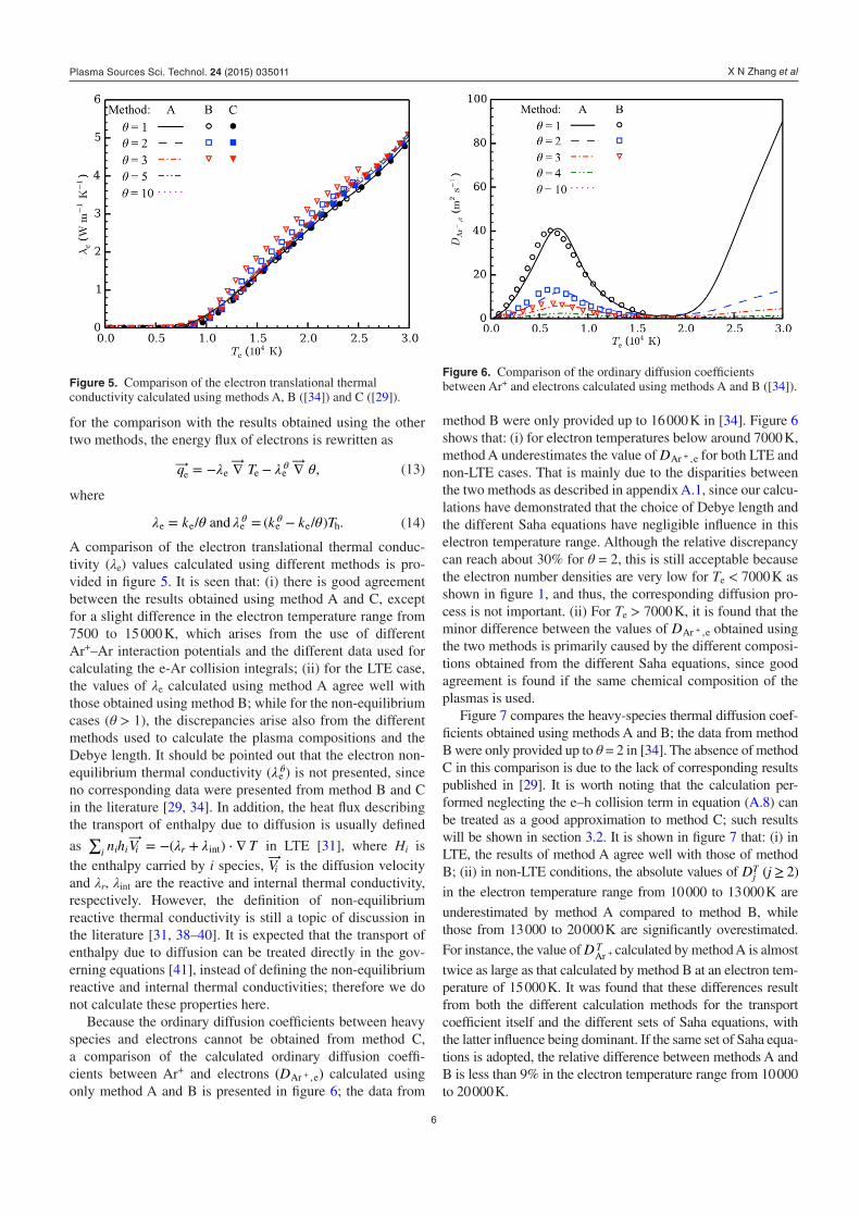
A comparison of the electron translational thermal conduc-tivity (λe) values calculated using different methods is pro-vided in figure 5. It is seen that: (i) there is good agreement between the results obtained using method A and C, except for a slight difference in the electron temperature range from 7500 to 15 000 K, which arises from the use of different Ar+–Ar interaction potentials and the different data used for calculating the e-Ar collision integrals; (ii) for the LTE case, the values of λe calculated using method A agree well with those obtained using method B; while for the non-equilibrium cases (θ > 1), the discrepancies arise also from the different methods used to calculate the plasma compositions and the Debye length. It should be pointed out that the electron non-equilibrium thermal conductivity (λ θ
e ) is not presented, since no corresponding data were presented from method B and C in the literature [29, 34]. In addition, the heat flux describing the transport of enthalpy due to diffusion is usually defined
as λ λ∑ = − + ⋅ ∇n h V T( )i i i i r int in LTE [31], where Hi is the enthalpy carried by i species, Vi is the diffusion velocity and λr, λint are the reactive and internal thermal conductivity, respectively. However, the definition of non-equilibrium reactive thermal conductivity is still a topic of discussion in the literature [31, 38–40]. It is expected that the transport of enthalpy due to diffusion can be treated directly in the gov-erning equations [41], instead of defining the non-equilibrium reactive and internal thermal conductivities; therefore we do not calculate these properties here.
Because the ordinary diffusion coefficients between heavy species and electrons cannot be obtained from method C, a comparison of the calculated ordinary diffusion coeffi-cients between Ar+ and electrons +D( )Ar ,e calculated using only method A and B is presented in figure 6; the data from
method B were only provided up to 16 000 K in [34]. Figure 6 shows that: (i) for electron temperatures below around 7000 K, method A underestimates the value of +DAr ,e for both LTE and non-LTE cases. That is mainly due to the disparities between the two methods as described in appendix A.1, since our calcu-lations have demonstrated that the choice of Debye length and the different Saha equations have negligible influence in this electron temperature range. Although the relative discrepancy can reach about 30% for θ = 2, this is still acceptable because the electron number densities are very low for Te < 7000 K as shown in figure 1, and thus, the corresponding diffusion pro-cess is not important. (ii) For Te > 7000 K, it is found that the minor difference between the values of +DAr ,e obtained using the two methods is primarily caused by the different composi-tions obtained from the different Saha equations, since good agreement is found if the same chemical composition of the plasmas is used.
Figure 7 compares the heavy-species thermal diffusion coef-ficients obtained using methods A and B; the data from method B were only provided up to θ = 2 in [34]. The absence of method C in this comparison is due to the lack of corresponding results published in [29]. It is worth noting that the calculation per-formed neglecting the e–h collision term in equation (A.8) can be treated as a good approximation to method C; such results will be shown in section 3.2. It is shown in figure 7 that: (i) in LTE, the results of method A agree well with those of method B; (ii) in non-LTE conditions, the absolute values of ≥D j( 2)j
T
in the electron temperature range from 10 000 to 13 000 K are
underestimated by method A compared to method B, while those from 13 000 to 20 000 K are significantly overestimated.
For instance, the value of +D TAr calculated by method A is almost
twice as large as that calculated by method B at an electron tem-perature of 15 000 K. It was found that these differences result from both the different calculation methods for the transport coefficient itself and the different sets of Saha equations, with the latter influence being dominant. If the same set of Saha equa-tions is adopted, the relative difference between methods A and B is less than 9% in the electron temperature range from 10 000 to 20 000 K.
Figure 5. Comparison of the electron translational thermal conductivity calculated using methods A, B ([34]) and C ([29]).
Figure 6. Comparison of the ordinary diffusion coefficients between Ar+ and electrons calculated using methods A and B ([34]).
Plasma Sources Sci. Technol. 24 (2015) 035011

X N Zhang et al
7
The mass conservation law requires that the sum of thermal diffusion coefficients of all species must vanish. Since the values of the electron thermal diffusion coefficient are very small, it is expected that the sum of the heavy-species thermal diffusion coefficients is approximately zero. From figure 7, we see that ≅ − ++ +D D D( ),T T T
Ar Ar Ar2 so this is indeed satisfied for both method A and method B.
A comparison of electron thermal diffusion coefficients calculated using methods A and B is presented in figure 8; data obtained by method C were also not published in [29]. In LTE, excellent agreement is observed between methods A and B, except for a slight difference at low temperatures due to the use of different collision integrals. For the non-equilib-rium cases, the discrepancies from method A and B arise (as shown in figure 8) from both the different Saha equations and the different definitions of Debye length, rather than the dif-ferent transport theories, since excellent agreement was found between the calculated values of DT
e from method A and B if the same formulas were used to calculate the chemical com-positions and Debye length of the plasmas.
3.2. Effects of the e–h collision term on the diffusion coefficients
We have argued that the e–h collision term in Boltzmann equa-tion for heavy species [equation (A.8)], which is neglected in method C, should play an important role in the calculation of the diffusion coefficients for heavy species. The influence of this term is considered in this section.
The ordinary diffusion coefficients +DAr ,e calculated with and without the e–h collision term are shown in figure 9(a). The e–h collision term has a large influence for all values of θ. For Te < 12 000 K and Te > 25 000 K the values of +DAr ,e are significantly underestimated when the e–h collision term is neglected, while they are overestimated for intermediate elec-tron temperatures. The relative discrepancy between the two cases reaches about 84% for the LTE case, and is smaller for 2-T plasmas, decreasing to about 60% for θ = 3.
A similar situation is observed for the heavy-species thermal diffusion coefficients D( )j
T as shown in figure 9(b).
A significant discrepancy exists between values calculated with and without the e–h collision term, and this discrep-ancy increases as the non-equilibrium degree increases. For example, the relative discrepancies between the values Dj
T (j = Ar or Ar+) obtained for the two cases at Te = 14 000 K are about 20, 38 and 58% for θ = 1, 2 and 3, respectively.
Since the e–h collision term only appears in the heavy-spe-cies Boltzmann equation [equation (A.8)], it will affect diffusion coefficients associated with heavy species, including the ordi-nary diffusion coefficients for heavy species and electrons and the heavy-species thermal diffusion coefficients, as illustrated in figures 9(a) and (b). There should be no influence on the diffu-sion coefficients of electrons, as is confirmed in figure 9(c).
It should be pointed out that the distribution functions of species appearing in the Boltzmann equation determine the macroscopic quantities of plasmas, such as the mass, momentum and energy fluxes [1, 2], and the e–h collision term in equation (A.8) represents the effects of collisions between electrons and heavy species on these quantities. It is well known that, due to the large mass of heavy species com-pared with that of electrons, neither the momentum nor the energy of a heavy particle is appreciably affected by collisions with electrons. Thus the viscosity and translational thermal conductivity calculated using method C, neglecting this e–h collision term, agree well with the results from method A and B, as shown in section 3.1. In contrast, the diffusion coeffi-cients of heavy species are significantly influenced by the e–h collision term, since the neglect of this term means that the mass exchange process between the sub-systems of electrons and heavy species is ignored, which is not physically correct.
4. Conclusions
Three main methods have been developed to calculate the transport coefficients of 2-T plasmas, namely the decoupled method of Devoto [13] (method C), the coupled method of Rat et al [16] (method B) and the new simplified method of Zhang et al [17] (method A). All are based on the Chapman–Enskog method of solving the Boltzmann equation. In this
Figure 7. Comparison of the thermal diffusion coefficients of heavy species calculated using methods A and B ([34]).
Figure 8. Comparison of the thermal diffusion coefficients of electrons calculated using methods A and B ([34]).
Plasma Sources Sci. Technol. 24 (2015) 035011

X N Zhang et al
8
paper, considerable effort has been devoted to the comparison of the calculated transport properties of 2-T argon plasmas using these three methods.
The main differences between the three methods have been carefully explained. In summary: (i) method C separates the calculation of electron and heavy-species transport coefficients completely by neglecting the interactions between electrons and heavy species, treating them as two isolated sub-systems to achieve a much-simplified calculation procedure; (ii) method
B does not make any simplifications, ensuring that the diffu-sion coefficients obtained are exact (within the assumptions of the Chapman–Enskog approach); while (iii) method A retains the physically reasonable simplifications of method C that are based on the physical fact that me << mh, while taking into account, as does method B, the coupling between the electrons and heavy species, to obtain accurate transport coefficients with a relatively simple calculation procedure.
The viscosity, electrical conductivity, thermal conduc-tivity and diffusion coefficients for argon plasmas have been calculated using method A under thermal equilibrium and non-equilibrium conditions at atmospheric pressure and for the electron temperature range from 300 to 30 000 K. These results have been compared with those obtained from the other two methods. It is found that all three methods give almost the same viscosity, electrical conductivity and trans-lational thermal conductivity for plasmas both in and out of LTE, except that method C slightly overestimates the elec-trical conductivity at high electron temperatures.
Since method A considers coupling between electrons and heavy species, it allows the calculation of ordinary diffu-sion coefficients between heavy species and electrons, unlike method C. The values obtained for ordinary diffusion coeffi-cients between Ar+ and e, and the thermal diffusion coefficients of heavy species, are slightly different from those obtained using method B because of the simplifications adopted in method A.
The electron–heavy-species collision term (e–h collision term) in the Boltzmann equation for heavy species was found to have a significant impact on the calculated values of the dif-fusion coefficients related to heavy species. In particular, the values of +DAr ,e calculated without considering the e–h colli-sion term show an incorrect dependence on electron tempera-ture. Further, without the e–h collision term, the values of the heavy-species thermal diffusion coefficients are significantly overestimated. Therefore, the e–h collision term is necessary to retain completeness of the species diffusion coefficients and to satisfy the mass conservation law in a plasma system.
Accurate diffusion coefficients are essential to a physically-correct treatment of the mass transfer processes in plasmas. We have demonstrated that the new simplified method of Zhang et al (method A) can be used for this purpose. This is an important advance, since it provides a major simplification over the method of Rat et al (method B), and since the method of Devoto (method C) does not allow a physically consistent set of diffusion coefficients to be calculated.
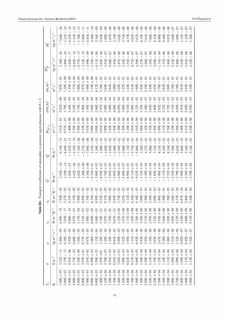
For convenient application of the newly calculated trans-port properties of 2-T argon plasmas, some of the argon plasma transport data are tabulated in the appendix. Please check the supplementary material (stacks.iop.org/PSST/24/035011/mmedia) or contact the corresponding authors for complete argon plasma transport property data in different pressure, temperature and temperature ratio ranges.
Acknowledgments
This work has been supported by the National Natural Sci-ence Foundation of China (Nos. 11035005, 11475174 and 50876101).
Figure 9. (a) Variations of the ordinary diffusion coefficients between Ar + and electrons, (b) thermal diffusion coefficients of heavy species, and (c) that of electrons with the electron temperature for the cases with or without the consideration of the e–h collision term in the heavy-species Boltzmann equation.
Plasma Sources Sci. Technol. 24 (2015) 035011
X N Zhang et al
9
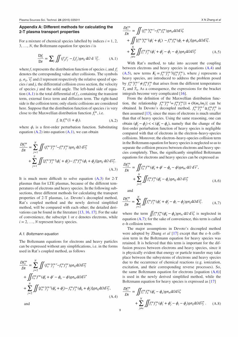
Appendix A: Different methods for calculating the 2-T plasma transport properties
For a mixture of chemical species labelled by indices i = 1, 2, 3, …, N, the Boltzmann equation for species i is
∬∑ σ= −′ ′ f
tf f f f g Ω v
D
D( ) d d ,i
j j j i j ij j (A.1)
where f i represents the distribution function of species i, and ′fi denotes the corresponding value after collisions. The symbols g, σij, vj and Ω represent respectively the relative speed of spe-cies i and j, the differential collision cross section, the velocity of species j and the solid angle. The left-hand side of equa-tion (A.1) is the total differential of f i, containing the transient term, external force term and diffusion term. The right-hand side is the collision term; only elastic collisions are considered here. Suppose that the distribution function of species i is very close to the Maxwellian distribution function f ,i
m i.e.
ϕ≅ +f f (1 ),i im
i (A.2)
where ϕi is a first-order perturbation function. Substituting equation (A.2) into equation (A.1), we can obtain
∬
∬
′ ′
′ ′
∑
∑
σ
ϕ ϕ ϕ ϕ σ
= −
+ + − +′ ′
=
=
Df
Dtf f f f g Ω v
f f f f g Ω v
( ) d d
[ ( ) ( )] d d .
im
j
N
im
jm
im
jm
ij j
j
N
im
jm
i j im
jm
i j ij j
1
1
(A.3)
It is much more difficult to solve equation (A.3) for 2-T plasmas than for LTE plasmas, because of the different tem-peratures of electrons and heavy species. In the following sub-sections, three different methods for calculating the transport properties of 2-T plasmas, i.e. Devoto’s decoupled method, Rat’s coupled method and the newly derived simplified method, will be compared with each other; the detailed deri-vations can be found in the literature [13, 16, 17]. For the sake of convenience, the subscript 1 or e denotes electrons, while i = 2, …, N represent heavy species.
A.1. Boltzmann equation
The Boltzmann equations for electrons and heavy particles can be expressed without any simplifications, i.e. in the forms used in Rat’s coupled method, as follows
∬
∬
∬
′ ′
′ ′
∑
∑
σ
ϕ ϕ ϕ ϕ σ
ϕ ϕ ϕ ϕ σ
= −
+ + − −
+ + − +
′ ′
′ ′
=
=
Df
Dtf f f f g Ω v
f f g Ω v
f f f f g Ω v
( ) d d
( ) d d
[ ( ) ( )] d d ,
m
j
Nm
jm m
jm
j j
m me e
j
Nm
jm
jm
jm
j j j
e
2e e e
e e e
2e e e e e
(A.4)
and
∬∬
∬
′ ′
′ ′
∑
σ
ϕ ϕ ϕ ϕ σ
ϕ ϕ ϕ ϕ σ
= −
+ + − +
+ + − −
′ ′
′ ′≠
Df
Dtf f f f g Ω v
f f f f g Ω v
f f g Ω v
( ) d d
[ ( ) ( )] d d .
( ) d d
im
im m
im m
i
im m
i im m
i i e
j
N
im
jm
i j i j ij j
e e e e
e e e e e
e
(A.5)
With Rat’s method, to take into account the coupling between electrons and heavy species in equations (A.4) and (A.5), new terms ′ ′=K f f f f/( ),j
mjm m
jm
e e where j represents a heavy species, are introduced to address the problem posed by ′ ′≠f f f fm
jm m
jm
e e that arises from the different temperatures Te and Th. As a consequence, the expressions for the bracket integrals become very complicated [16].
From the definition of the Maxwellian distribution func-tion, the relationship ′ ′= +f f f f O m m[1 ( / )]m
jm m
jm
e je e can be obtained. In Devoto’s decoupled method, ′ ′≅f f f fm
jm m
jm
e e is then assumed [13], since the mass of electrons is much smaller than that of heavy species. Using the same reasoning, one can obtain ϕ ϕ ϕ ϕ− < < −′ ′( ) ( ),j j e e namely that the change of the first-order perturbation function of heavy species is negligible compared with that of electrons in the electron–heavy-species collisions. Moreover, the electron–heavy-species collision term in the Boltzmann equation for heavy species is neglected so as to separate the collision process between electrons and heavy spe-cies completely. Thus, the significantly simplified Boltzmann equations for electrons and heavy species can be expressed as
∬
∬∑
ϕ ϕ ϕ ϕ σ
ϕ ϕ σ
= + − −
+ −
′ ′
′=
Df
Dtf f g Ω v
f f g Ω v
( ) d d ,
( ) d d
mm m
j
Nm
jm
e e j j
ee e e ee
2e e
(A.6)
and
∬∑ ϕ ϕ ϕ ϕ σ= + − −′ ′=
Df
Dtf f g Ω v( ) d d ,i
m
j
N
im
jm
i j i j ij j
2
(A.7)
where the term ∬ ϕ ϕ σ−′ f f g Ω v( ) d dim m
ie e e e e is neglected in equation (A.7); for the sake of convenience, this term is called e–h collision term.
The major assumptions in Devoto’s decoupled method were adopted by Zhang et al [17] except that the e–h colli-sion term in the Boltzmann equation for heavy species was retained. It is believed that this term is important for the dif-fusion process between electrons and heavy species, since it is physically evident that energy or particle transfer may take place between the subsystems of electrons and heavy species due to the occurrence of chemical reactions (e.g. ionization, excitation, and their corresponding reverse processes). So, the same Boltzmann equation for electrons [equation (A.6)] is used in the newly derived simplified method, while the Boltzmann equation for heavy species is expressed as [17]
∬
∬∑
ϕ ϕ σ
ϕ ϕ ϕ ϕ σ
= −
+ + − −
′
′ ′≠
Df
Dtf f g Ω v
f f g Ω v
( ) d d
( ) d d .
im
im m
i
j
N
im
jm
i j i j ij j
e e e e e
e
(A.8)
Plasma Sources Sci. Technol. 24 (2015) 035011

X N Zhang et al
10
Such a treatment method does not make the calculations for electron transport properties more complex than Devoto’s method, since the Boltzmann equation for electrons can still be solved separately, and the results of this calculation are then used to solve the Boltzmann equation for heavy species [equation (A.8)], taking into account the energy exchange processes between electrons and heavy species.
A.2. Expressions for the first-order perturbation function
In order to solve the preceding species Boltzmann equations, an appropriate expression for ϕi has to be assumed. In Rat’s coupled method [16] and the new simplified method [17], the following form for the perturbation function is employed
∑
∑
ϕ
ω θ θ
= − ⋅ ∇ −↔
∇ + ⋅ +
+ ⋅ ∇ − ⋅
=
=
A T B v C d D Q
E F
ln :
ln ln ,
i i ij
N
ij
j i
j
N
ij
j i
h 01
e(0)
1
(A.9)
where v0 is the mass-averaged velocity, dj is the diffusion driving force acting on species j, θ is the temperature ratio of electrons and heavy species, i.e. θ = Te / Th, which is treated as a function of the space vector r( ), i.e.
θ∇ = ∇ + ∇ T Tln ln ln ,e h (A.10)
and the physical meanings of other variables can be found in [16, 17].
It is noted that ∑ ⋅= C djN
ij
j1 in equation (A.9) is directly
related to the calculation of the ordinary diffusion coefficients, and the sum of j is from 1 to N to guarantee the completeness of the ordinary diffusion coefficients. However, in Devoto’s decoupled method [13], the diffusion process between elec-trons and heavy species is neglected and the forms of ϕe and ϕi (i = 2, …, N) are given, respectively, by
ϕ = − ⋅ ∇ −↔
∇ + ⋅⎯→
+′ A T B v C d D Qln : ,e e e e 0 e e e e(0) (A.11)
∑ϕ = − ⋅ ∇ −↔
∇ + ⋅ +′=
A T B v C d D Qln : .i i i
j
N
ij
j ih 0
2
e(0)
(A.12)
Here, the definition of the diffusion driving force is dif-ferent from that appearing in equation (A.9) [16, 17], i.e.
≠′d d ;j j and the temperature ratio, θ, is defined as a constant, i.e.
∇ = ∇ T Tln ln .e h (A.13)
A.3. Momentum conservation
In a plasma system, the sum of all momentum fluxes must vanish according to the momentum conservation law. Thus, the following condition must be employed in the derivation of the plasma transport properties:
∫∑ ϕ ==
m v f vd 0.i
N
i i im
i i
1
(A.14)
It is seen clearly from the derivations presented in [16, 17] that equation (A.14) has been used; while in the derivation of Devoto’s decoupled method, the momentum flux of electrons is omitted, namely,
∫∑ ϕ ==
m v f vd 0,i
N
i i im
i i
2
(A.15)
which means that the physical constraint [equation (A.14)] is not satisfied in the calculation of the species diffusion coef-ficients based on the decoupled method.
A.4. Formulas for transport coefficients
Here, for the completeness of this paper, the formulas of some transport coefficients based on the new method proposed by Zhang et al are presented.
Electrical conductivity:
∑σ ==
e n
mn Z
Q Q
Q Q
Q
3
2,
j
N
j j mn
2e
e 2
111
112
121
122
1
(A.16)
and
=Q
Q Q Q
Q Q Q
Q Q Q
,mn1
111
112
113
121
122
123
131
132
133
(A.17)
Viscosity:
=
−
− −− −
μ k n T
b k T
Q Q n Q b Q b
Q Q n Q b Q b
n
Q Q
Q Q
1
2
1
2
5 * *
5 * *
0 0,
ij ij i i i
ij ij i i i
j
ij ij
ij ij
B e e
10 B h
00 01100
10 101
11
10 11110
10 111
11
00 01
10 11
(A.18)
where
=⋯
⋮ ⋯ ⋮⋯
QQ Q
Q Q,ij
mn
mnN
mn
Nmn
NNmn
22 2
2
(A.19)
=−
=−
bn Q
Q Q Q Qb
n Q
Q Q Q Q
5and
5.10
e 111
100
111
110
101 11
e 110
110
101
100
111
(A.20)
The elements of the determinants, Q Q,mnijmn
1 and Q ,mn1
* can be calculated as presented in [2, 13]. Since all the expressions of transport coefficients have been described in [17], it is not necessary to reproduce all of them here. The interested reader can refer to [17].
Plasma Sources Sci. Technol. 24 (2015) 035011
X N Zhang et al
11
Ap
pen
dix
B: T
ran
spo
rt p
rop
erti
es o
f at
mo
sph
eric
arg
on
pla
smas
wit
h d
iffer
ent
tem
per
atu
re r
atio
s
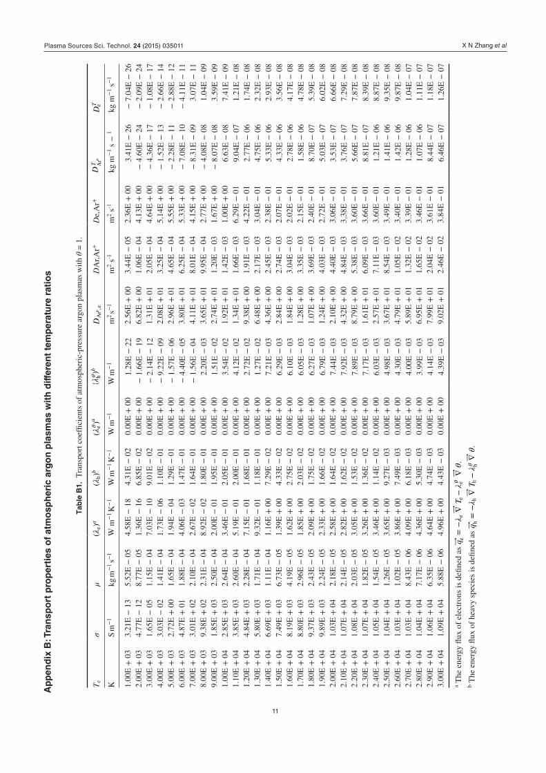
Tab
le B
1. T
rans
port
coe
ffici
ents
of
atm
osph
eric
-pre
ssur
e ar
gon
plas
mas
with
θ =
1.
Te
σμ
λ()a
eλ(
)bh
λθ(
)ae
λθ(
)bh
+D
Ar
,eD
Ar,A
r+D
e,A
r++
DT A
rD
T e
KS
m−
1kg
m−
1 s−1
W m
−1 K
−1
W m
−1 K
−1
W m
−1
W m
−1
m2 s−
1m
2 s-1
m2 s
-1kg
m−
1 s −
1kg
m−
1 s−
1
1.00
E +
03
3.21
E −
13
5.52
E −
05
4.58
E −
18
4.31
E −
02
0.00
E +
00
1.28
E −
22
2.56
E +
00
3.44
E −
05
2.36
E +
00
3.41
E −
26
− 7
.04E
− 2
62.
00E
+ 0
34.
77E
− 1
28.
77E
− 0
51.
36E
− 1
66.
85E
− 0
20.
00E
+ 0
0−
1.6
6E −
19
6.82
E +
00
1.06
E −
04
4.13
E +
00
− 4
.60E
− 2
4 −
2.0
9E −
24
3.00
E +
03
1.65
E −
05
1.15
E −
04
7.03
E −
10
9.01
E −
02
0.00
E +
00
− 2
.14E
− 1
21.
31E
+ 0
12.
05E
− 0
44.
64E
+ 0
0 −
4.3
6E −
17
− 1
.08E
− 1
74.
00E
+ 0
33.
03E
− 0
21.
41E
− 0
41.
73E
− 0
61.
10E
− 0
10.
00E
+ 0
0−
9.2
2E −
09
2.08
E +
01
3.25
E −
04
5.14
E +
00
− 1
.52E
− 1
3 −
2.6
6E −
14
5.00
E +
03
2.72
E +
00
1.65
E −
04
1.94
E −
04
1.29
E −
01
0.00
E +
00
− 1
.57E
− 0
62.
96E
+ 0
14.
65E
− 0
45.
55E
+ 0
0 −
2.2
8E −
11
− 2
.88E
− 1
26.
00E
+ 0
34.
87E
+ 0
11.
88E
− 0
44.
06E
− 0
31.
47E
− 0
10.
00E
+ 0
0−
4.4
0E −
05
3.80
E +
01
6.25
E −
04
5.33
E +
00
− 7
.08E
− 1
0 −
4.1
1E −
11
7.00
E +
03
3.01
E +
02
2.10
E −
04
2.67
E −
02
1.64
E −
01
0.00
E +
00
− 1
.56E
− 0
44.
11E
+ 0
18.
01E
− 0
44.
15E
+ 0
0 −
8.3
1E −
09
3.07
E −
11
8.00
E +
03
9.38
E +
02
2.31
E −
04
8.92
E −
02
1.80
E −
01
0.00
E +
00
2.20
E −
03
3.65
E +
01
9.95
E −
04
2.77
E +
00
− 4
.08E
− 0
81.
04E
− 0
99.
00E
+ 0
31.
85E
+ 0
32.
50E
− 0
42.
00E
− 0
11.
95E
− 0
10.
00E
+ 0
01.
51E
− 0
22.
74E
+ 0
11.
20E
− 0
31.
67E
+ 0
0 −
8.0
7E −
08
3.59
E −
09
1.00
E +
04
2.85
E +
03
2.64
E −
04
3.46
E −
01
2.05
E −
01
0.00
E +
00
3.54
E −
02
1.92
E +
01
1.42
E −
03
1.00
E +
00
6.63
E −
08
7.41
E −
09
1.10
E +
04
3.85
E +
03
2.60
E −
04
5.19
E −
01
2.00
E −
01
0.00
E +
00
4.12
E −
02
1.34
E +
01
1.66
E −
03
6.29
E −
01
9.04
E −
07
1.21
E −
08
1.20
E +
04
4.84
E +
03
2.28
E −
04
7.15
E −
01
1.68
E −
01
0.00
E +
00
2.72
E −
02
9.38
E +
00
1.91
E −
03
4.22
E −
01
2.77
E −
06
1.74
E −
08
1.30
E +
04
5.80
E +
03
1.71
E −
04
9.32
E −
01
1.18
E −
01
0.00
E +
00
1.27
E −
02
6.48
E +
00
2.17
E −
03
3.04
E −
01
4.75
E −
06
2.32
E −
08
1.40
E +
04
6.69
E +
03
1.11
E −
04
1.16
E +
00
7.29
E −
02
0.00
E +
00
7.21
E −
03
4.36
E +
00
2.45
E −
03
2.38
E −
01
5.33
E −
06
2.93
E −
08
1.50
E +
04
7.49
E +
03
6.73
E −
05
1.39
E +
00
4.33
E −
02
0.00
E +
00
6.29
E −
03
2.84
E +
00
2.74
E −
03
2.07
E −
01
4.33
E −
06
3.56
E −
08
1.60
E +
04
8.19
E +
03
4.19
E −
05
1.62
E +
00
2.75
E −
02
0.00
E +
00
6.10
E −
03
1.84
E +
00
3.04
E −
03
2.02
E −
01
2.78
E −
06
4.17
E −
08
1.70
E +
04
8.80
E +
03
2.96
E −
05
1.85
E +
00
2.03
E −
02
0.00
E +
00
6.05
E −
03
1.28
E +
00
3.35
E −
03
2.15
E −
01
1.58
E −
06
4.78
E −
08
1.80
E +
04
9.37
E +
03
2.43
E −
05
2.09
E +
00
1.75
E −
02
0.00
E +
00
6.27
E −
03
1.07
E +
00
3.69
E −
03
2.40
E −
01
8.70
E −
07
5.39
E −
08
1.90
E +
04
9.89
E +
03
2.24
E −
05
2.33
E +
00
1.66
E −
02
0.00
E +
00
6.79
E −
03
1.24
E +
00
4.03
E −
03
2.72
E −
01
5.03
E −
07
6.02
E −
08
2.00
E +
04
1.03
E +
04
2.18
E −
05
2.58
E +
00
1.64
E −
02
0.00
E +
00
7.44
E −
03
2.10
E +
00
4.40
E −
03
3.06
E −
01
3.53
E −
07
6.66
E −
08
2.10
E +
04
1.07
E +
04
2.14
E −
05
2.82
E +
00
1.62
E −
02
0.00
E +
00
7.92
E −
03
4.32
E +
00
4.84
E −
03
3.38
E −
01
3.76
E −
07
7.29
E −
08
2.20
E +
04
1.08
E +
04
2.03
E −
05
3.05
E +
00
1.53
E −
02
0.00
E +
00
7.89
E −
03
8.79
E +
00
5.38
E −
03
3.60
E −
01
5.66
E −
07
7.87
E −
08
2.30
E +
04
1.07
E +
04
1.82
E −
05
3.26
E +
00
1.36
E −
02
0.00
E +
00
7.17
E −
03
1.61
E +
01
6.09
E −
03
3.66
E −
01
8.81
E −
07
8.39
E −
08
2.40
E +
04
1.05
E +
04
1.54
E −
05
3.46
E +
00
1.14
E −
02
0.00
E +
00
6.03
E −
03
2.57
E +
01
7.11
E −
03
3.60
E −
01
1.21
E −
06
8.87
E −
08
2.50
E +
04
1.04
E +
04
1.26
E −
05
3.65
E +
00
9.27
E −
03
0.00
E +
00
4.98
E −
03
3.67
E +
01
8.54
E −
03
3.49
E −
01
1.41
E −
06
9.35
E −
08
2.60
E +
04
1.03
E +
04
1.02
E −
05
3.86
E +
00
7.49
E −
03
0.00
E +
00
4.30
E −
03
4.79
E +
01
1.05
E −
02
3.40
E −
01
1.42
E −
06
9.87
E −
08
2.70
E +
04
1.03
E +
04
8.43
E −
06
4.09
E +
00
6.18
E −
03
0.00
E +
00
4.00
E −
03
5.89
E +
01
1.32
E −
02
3.39
E −
01
1.28
E −
06
1.04
E −
07
2.80
E +
04
1.04
E +
04
7.17
E −
06
4.36
E +
00
5.30
E −
03
0.00
E +
00
3.99
E −
03
6.95
E +
01
1.65
E −
02
3.46
E −
01
1.07
E −
06
1.11
E −
07
2.90
E +
04
1.06
E +
04
6.35
E −
06
4.64
E +
00
4.74
E −
03
0.00
E +
00
4.14
E −
03
7.99
E +
01
2.04
E −
02
3.61
E −
01
8.44
E −
07
1.18
E −
07
3.00
E +
04
1.09
E +
04
5.88
E −
06
4.96
E +
00
4.43
E −
03
0.00
E +
00
4.39
E −
03
9.02
E +
01
2.46
E −
02
3.84
E −
01
6.46
E −
07
1.26
E −
07
a The
ene
rgy
flux
of e
lect
rons
is d
efine
d as
λ
λθ
=−
∇−
∇θ
q
T.
ee
ee
b The
ene
rgy
flux
of h
eavy
spe
cies
is d
efine
d as
λ
λθ
=−
∇−
∇θ
q
T.
hh
hh
Plasma Sources Sci. Technol. 24 (2015) 035011
X N Zhang et al
12
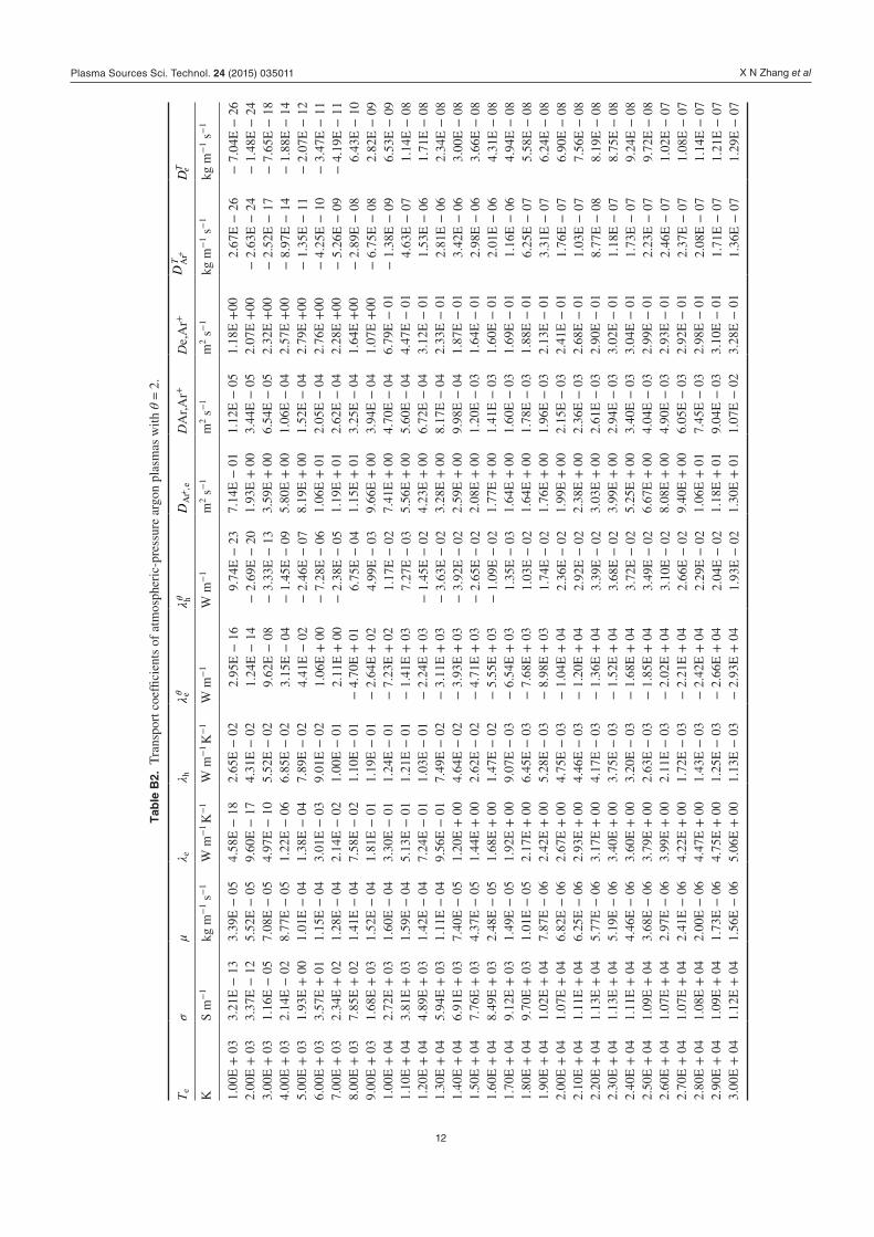
Tab
le B
2. T
rans
port
coe
ffici
ents
of
atm
osph
eric
-pre
ssur
e ar
gon
plas
mas
with
θ =
2.
Te
σμ
λ eλ h
λθ eλθ h
+D
Ar
,eD
Ar,A
r+D
e,A
r++
DT A
rD
eT
KS
m−
1kg
m−
1 s−
1W
m−
1 K−
1W
m−
1 K−
1W
m−
1W
m−
1m
2 s−
1m
2 s−
1m
2 s−
1kg
m−
1 s−
1kg
m−
1 s−
1
1.00
E +
03
3.21
E −
13
3.39
E −
05
4.58
E −
18
2.65
E −
02
2.95
E −
16
9.74
E −
23
7.14
E −
01
1.12
E −
05
1.18
E +
002.
67E
− 2
6 −
7.0
4E −
26
2.00
E +
03
3.37
E −
12
5.52
E −
05
9.60
E −
17
4.31
E −
02
1.24
E −
14
− 2
.69E
− 2
01.
93E
+ 0
03.
44E
− 0
52.
07E
+00
− 2
.63E
− 2
4 −
1.4
8E −
24
3.00
E +
03
1.16
E −
05
7.08
E −
05
4.97
E −
10
5.52
E −
02
9.62
E −
08
− 3
.33E
− 1
33.
59E
+ 0
06.
54E
− 0
52.
32E
+00
− 2
.52E
− 1
7 −
7.6
5E −
18
4.00
E +
03
2.14
E −
02
8.77
E −
05
1.22
E −
06
6.85
E −
02
3.15
E −
04
− 1
.45E
− 0
95.
80E
+ 0
01.
06E
− 0
42.
57E
+00
− 8
.97E
− 1
4 −
1.8
8E −
14
5.00
E +
03
1.93
E +
00
1.01
E −
04
1.38
E −
04
7.89
E −
02
4.41
E −
02
− 2
.46E
− 0
78.
19E
+ 0
01.
52E
− 0
42.
79E
+00
− 1
.35E
− 1
1 −
2.0
7E −
12
6.00
E +
03
3.57
E +
01
1.15
E −
04
3.01
E −
03
9.01
E −
02
1.06
E +
00
− 7
.28E
− 0
61.
06E
+ 0
12.
05E
− 0
42.
76E
+00
− 4
.25E
− 1
0 −
3.4
7E −
11
7.00
E +
03
2.34
E +
02
1.28
E −
04
2.14
E −
02
1.00
E −
01
2.11
E +
00
− 2
.38E
− 0
51.
19E
+ 0
12.
62E
− 0
42.
28E
+00
− 5
.26E
− 0
9 −
4.1
9E −
11
8.00
E +
03
7.85
E +
02
1.41
E −
04
7.58
E −
02
1.10
E −
01
− 4
.70E
+ 0
16.
75E
− 0
41.
15E
+ 0
13.
25E
− 0
41.
64E
+00
− 2
.89E
− 0
86.
43E
− 1
09.
00E
+ 0
31.
68E
+ 0
31.
52E
− 0
41.
81E
− 0
11.
19E
− 0
1 −
2.6
4E +
02
4.99
E −
03
9.66
E +
00
3.94
E −
04
1.07
E +
00 −
6.7
5E −
08
2.82
E −
09
1.00
E +
04
2.72
E +
03
1.60
E −
04
3.30
E −
01
1.24
E −
01
− 7
.23E
+ 0
21.
17E
− 0
27.
41E
+ 0
04.
70E
− 0
46.
79E
− 0
1 −
1.3
8E −
09
6.53
E −
09
1.10
E +
04
3.81
E +
03
1.59
E −
04
5.13
E −
01
1.21
E −
01
− 1
.41E
+ 0
37.
27E
− 0
35.
56E
+ 0
05.
60E
− 0
44.
47E
− 0
14.
63E
− 0
71.
14E
− 0
81.
20E
+ 0
44.
89E
+ 0
31.
42E
− 0
47.
24E
− 0
11.
03E
− 0
1 −
2.2
4E +
03
− 1
.45E
− 0
24.
23E
+ 0
06.
72E
− 0
43.
12E
− 0
11.
53E
− 0
61.
71E
− 0
81.
30E
+ 0
45.
94E
+ 0
31.
11E
− 0
49.
56E
− 0
17.
49E
− 0
2 −
3.1
1E +
03
− 3
.63E
− 0
23.
28E
+ 0
08.
17E
− 0
42.
33E
− 0
12.
81E
− 0
62.
34E
− 0
81.
40E
+ 0
46.
91E
+ 0
37.
40E
− 0
51.
20E
+ 0
04.
64E
− 0
2 −
3.9
3E +
03
− 3
.92E
− 0
22.
59E
+ 0
09.
98E
− 0
41.
87E
− 0
13.
42E
− 0
63.
00E
− 0
81.
50E
+ 0
47.
76E
+ 0
34.
37E
− 0
51.
44E
+ 0
02.
62E
− 0
2 −
4.7
1E +
03
− 2
.65E
− 0
22.
08E
+ 0
01.
20E
− 0
31.
64E
− 0
12.
98E
− 0
63.
66E
− 0
81.
60E
+ 0
48.
49E
+ 0
32.
48E
− 0
51.
68E
+ 0
01.
47E
− 0
2 −
5.5
5E +
03
− 1
.09E
− 0
21.
77E
+ 0
01.
41E
− 0
31.
60E
− 0
12.
01E
− 0
64.
31E
− 0
81.
70E
+ 0
49.
12E
+ 0
31.
49E
− 0
51.
92E
+ 0
09.
07E
− 0
3 −
6.5
4E +
03
1.35
E −
03
1.64
E +
00
1.60
E −
03
1.69
E −
01
1.16
E −
06
4.94
E −
08
1.80
E +
04
9.70
E +
03
1.01
E −
05
2.17
E +
00
6.45
E −
03
− 7
.68E
+ 0
31.
03E
− 0
21.
64E
+ 0
01.
78E
− 0
31.
88E
− 0
16.
25E
− 0
75.
58E
− 0
81.
90E
+ 0
41.
02E
+ 0
47.
87E
− 0
62.
42E
+ 0
05.
28E
− 0
3 −
8.9
8E +
03
1.74
E −
02
1.76
E +
00
1.96
E −
03
2.13
E −
01
3.31
E −
07
6.24
E −
08
2.00
E +
04
1.07
E +
04
6.82
E −
06
2.67
E +
00
4.75
E −
03
− 1
.04E
+ 0
42.
36E
− 0
21.
99E
+ 0
02.
15E
− 0
32.
41E
− 0
11.
76E
− 0
76.
90E
− 0
82.
10E
+ 0
41.
11E
+ 0
46.
25E
− 0
62.
93E
+ 0
04.
46E
− 0
3 −
1.2
0E +
04
2.92
E −
02
2.38
E +
00
2.36
E −
03
2.68
E −
01
1.03
E −
07
7.56
E −
08
2.20
E +
04
1.13
E +
04
5.77
E −
06
3.17
E +
00
4.17
E −
03
− 1
.36E
+ 0
43.
39E
− 0
23.
03E
+ 0
02.
61E
− 0
32.
90E
− 0
18.
77E
− 0
88.
19E
− 0
82.
30E
+ 0
41.
13E
+ 0
45.
19E
− 0
63.
40E
+ 0
03.
75E
− 0
3 −
1.5
2E +
04
3.68
E −
02
3.99
E +
00
2.94
E −
03
3.02
E −
01
1.18
E −
07
8.75
E −
08
2.40
E +
04
1.11
E +
04
4.46
E −
06
3.60
E +
00
3.20
E −
03
− 1
.68E
+ 0
43.
72E
− 0
25.
25E
+ 0
03.
40E
− 0
33.
04E
− 0
11.
73E
− 0
79.
24E
− 0
82.
50E
+ 0
41.
09E
+ 0
43.
68E
− 0
63.
79E
+ 0
02.
63E
− 0
3 −
1.8
5E +
04
3.49
E −
02
6.67
E +
00
4.04
E −
03
2.99
E −
01
2.23
E −
07
9.72
E −
08
2.60
E +
04
1.07
E +
04
2.97
E −
06
3.99
E +
00
2.11
E −
03
− 2
.02E
+ 0
43.
10E
− 0
28.
08E
+ 0
04.
90E
− 0
32.
93E
− 0
12.
46E
− 0
71.
02E
− 0
72.
70E
+ 0
41.
07E
+ 0
42.
41E
− 0
64.
22E
+ 0
01.
72E
− 0
3 −
2.2
1E +
04
2.66
E −
02
9.40
E +
00
6.05
E −
03
2.92
E −
01
2.37
E −
07
1.08
E −
07
2.80
E +
04
1.08
E +
04
2.00
E −
06
4.47
E +
00
1.43
E −
03
− 2
.42E
+ 0
42.
29E
− 0
21.
06E
+ 0
17.
45E
− 0
32.
98E
− 0
12.
08E
− 0
71.
14E
− 0
72.
90E
+ 0
41.
09E
+ 0
41.
73E
− 0
64.
75E
+ 0
01.
25E
− 0
3 −
2.6
6E +
04
2.04
E −
02
1.18
E +
01
9.04
E −
03
3.10
E −
01
1.71
E −
07
1.21
E −
07
3.00
E +
04
1.12
E +
04
1.56
E −
06
5.06
E +
00
1.13
E −
03
− 2
.93E
+ 0
41.
93E
− 0
21.
30E
+ 0
11.
07E
− 0
23.
28E
− 0
11.
36E
− 0
71.
29E
− 0
7
Plasma Sources Sci. Technol. 24 (2015) 035011
X N Zhang et al
13
Tab
le B
3. T
rans
port
coe
ffici
ents
of
atm
osph
er ic
-pre
ssur
e ar
gon
plas
mas
with
θ =
3.
Te
σμ
λ eλ h
λθ eλθ h
+D
Ar
,eD
Ar,A
r+D
e,A
r++
DT A
rD
T e
KS
m−
1kg
m−
1 s−
1W
m−
1 K−
1W
m−
1 K−
1W
m−
1W
m−
1m
2 s−
1m
2 s–1
m2 s
–1kg
m–1
s–1
kg m
–1 s
–1
1.00
E +
03
3.21
E −
13
2.46
E −
05
4.58
E −
18
1.92
E −
02
3.93
E −
16
6.33
E −
23
3.51
E −
01
5.81
E −
06
7.85
E −
01
2.18
E −
26
− 7
.04E
− 2
62.
00E
+ 0
32.
75E
− 1
24.
19E
− 0
57.
84E
− 1
73.
27E
− 0
21.
35E
− 1
4 −
8.4
4E −
21
9.57
E −
01
1.79
E −
05
1.38
E +
00
− 1
.89E
− 2
4 −
1.2
1E −
24
3.00
E +
03
9.51
E −
06
5.52
E −
05
4.06
E −
10
4.31
E −
02
1.05
E −
07
− 1
.07E
− 1
31.
80E
+ 0
03.
44E
− 0
51.
55E
+ 0
0 −
1.8
2E −
17
− 6
.25E
− 1
84.
00E
+ 0
31.
75E
− 0
26.
60E
− 0
59.
97E
− 0
75.
15E
− 0
23.
43E
− 0
4 −
4.3
5E −
10
2.78
E +
00
5.43
E −
05
1.71
E +
00
− 6
.45E
− 1
4 −
1.5
3E −
14
5.00
E +
03
1.58
E +
00
7.56
E −
05
1.13
E −
04
5.90
E −
02
4.82
E −
02
− 7
.24E
− 0
83.
90E
+ 0
07.
74E
− 0
51.
86E
+ 0
0 −
9.7
7E −
12
− 1
.70E
− 1
26.
00E
+ 0
32.
97E
+ 0
18.
77E
− 0
52.
51E
− 0
36.
85E
− 0
21.
20E
+ 0
0 −
2.2
7E −
06
5.19
E +
00
1.06
E −
04
1.87
E +
00
− 3
.12E
− 1
0 −
3.0
6E −
11
7.00
E +
03
2.01
E +
02
9.67
E −
05
1.86
E −
02
7.55
E −
02
4.34
E +
00
− 7
.84E
− 0
65.
93E
+ 0
01.
36E
− 0
41.
60E
+ 0
0 −
3.9
9E −
09
− 6
.81E
− 1
18.
00E
+ 0
36.
99E
+ 0
21.
06E
− 0
46.
84E
− 0
28.
23E
− 0
2 −
4.2
1E +
01
2.47
E −
04
5.86
E +
00
1.69
E −
04
1.19
E +
00
− 2
.33E
− 0
84.
48E
− 1
09.
00E
+ 0
31.
56E
+ 0
31.
15E
− 0
41.
68E
− 0
18.
95E
− 0
2 −
2.8
6E +
02
1.56
E −
03
5.09
E +
00
2.06
E −
04
8.12
E −
01
− 6
.11E
− 0
82.
36E
− 0
91.
00E
+ 0
42.
63E
+03
1.20
E −
04
3.18
E −
01
9.33
E −
02
− 8
.54E
+ 0
21.
89E
− 0
34.
01E
+ 0
02.
47E
− 0
45.
36E
− 0
1 −
3.6
5E −
08
5.93
E −
09
1.10
E +
04
3.76
E +
03
1.20
E −
04
5.07
E −
01
9.13
E −
02
− 1
.74E
+ 0
3 −
4.6
8E −
03
3.09
E +
00
2.98
E −
04
3.64
E −
01
2.51
E −
07
1.08
E −
08
1.20
E +
04
4.91
E +
03
1.10
E −
04
7.25
E −
01
7.98
E −
02
− 2
.83E
+ 0
3 −
1.8
5E −
02
2.42
E +
00
3.68
E −
04
2.61
E −
01
9.68
E −
07
1.67
E −
08
1.30
E +
04
6.01
E +
03
8.81
E −
05
9.67
E −
01
5.93
E −
02
− 3
.95E
+ 0
3 −
2.9
6E −
02
1.94
E +
00
4.68
E −
04
2.00
E −
01
1.91
E −
06
2.33
E −
08
1.40
E +
04
7.02
E +
03
5.99
E −
05
1.22
E +
00
3.73
E −
02
− 4
.96E
+ 0
3 −
2.9
4E −
02
1.58
E +
00
6.05
E −
04
1.65
E −
01
2.47
E −
06
3.03
E −
08
1.50
E +
04
7.89
E +
03
3.53
E −
05
1.47
E +
00
2.07
E −
02
− 5
.89E
+ 0
3 −
2.0
6E −
02
1.29
E +
00
7.68
E −
04
1.47
E −
01
2.24
E −
06
3.71
E −
08
1.60
E +
04
8.62
E +
03
1.95
E −
05
1.71
E +
00
1.12
E −
02
− 6
.90E
+ 0
3 −
1.1
3E −
02
1.10
E +
00
9.32
E −
04
1.44
E −
01
1.53
E −
06
4.37
E −
08
1.70
E +
04
9.27
E +
03
1.11
E −
05
1.95
E +
00
6.42
E −
03
− 8
.11E
+ 0
3 −
4.7
3E −
03
1.01
E +
00
1.08
E −
03
1.53
E −
01
8.77
E −
07
5.02
E −
08
1.80
E +
04
9.86
E +
03
6.93
E −
06
2.20
E +
00
4.16
E −
03
− 9
.52E
+ 0
3 −
5.8
0E −
04
1.01
E +
00
1.22
E −
03
1.69
E −
01
4.59
E −
07
5.67
E −
08
1.90
E +
04
1.04
E +
04
4.93
E −
06
2.45
E +
00
3.09
E −
03
− 1
.11E
+ 0
42.
20E
− 0
31.
06E
+ 0
01.
35E
− 0
31.
92E
− 0
12.
27E
− 0
76.
33E
− 0
82.
00E
+ 0
41.
09E
+ 0
43.
93E
− 0
62.
71E
+ 0
02.
58E
− 0
3 −
1.2
9E +
04
4.27
E −
03
1.16
E +
00
1.48
E −
03
2.18
E −
01
1.00
E −
07
7.01
E −
08
2.10
E +
04
1.13
E +
04
3.39
E −
06
2.97
E +
00
2.29
E −
03
− 1
.48E
+ 0
45.
96E
− 0
31.
32E
+ 0
01.
63E
− 0
32.
44E
− 0
13.
25E
− 0
87.
68E
− 0
82.
20E
+ 0
41.
15E
+ 0
43.
02E
− 0
63.
22E
+ 0
02.
08E
− 0
3 −
1.6
9E +
04
7.32
E −
03
1.56
E +
00
1.80
E −
03
2.65
E −
01
2.03
E −
09
8.32
E −
08
2.30
E +
04
1.15
E +
04
2.67
E −
06
3.45
E +
00
1.86
E −
03
− 1
.90E
+ 0
48.
23E
− 0
31.
89E
+ 0
02.
02E
− 0
32.
79E
− 0
1 −
1.3
1E −
09
8.90
E −
08
2.40
E +
04
1.14
E +
04
2.28
E −
06
3.66
E +
00
1.58
E −
03
− 2
.11E
+ 0
48.
54E
− 0
32.
31E
+ 0
02.
33E
− 0
32.
83E
− 0
11.
37E
− 0
89.
40E
− 0
82.
50E
+ 0
41.
11E
+ 0
41.
88E
− 0
63.
85E
+ 0
01.
30E
− 0
3 −
2.3
2E +
04
8.24
E −
03
2.76
E +
00
2.75
E −
03
2.80
E −
01
3.49
E −
08
9.87
E −
08
2.60
E +
04
1.09
E +
04
1.51
E −
06
4.05
E +
00
1.04
E −
03
− 2
.54E
+ 0
47.
50E
− 0
33.
19E
+ 0
03.
31E
− 0
32.
76E
− 0
15.
12E
− 0
81.
04E
− 0
72.
70E
+ 0
41.
09E
+ 0
41.
22E
− 0
64.
27E
+ 0
08.
37E
− 0
4 −
2.7
9E +
04
6.62
E −
03
3.56
E +
00
4.04
E −
03
2.76
E −
01
5.80
E −
08
1.09
E −
07
2.80
E +
04
1.09
E +
04
9.95
E −
07
4.52
E +
00
6.87
E −
04
− 3
.06E
+ 0
45.
86E
− 0
33.
90E
+ 0
04.
91E
− 0
32.
81E
− 0
15.
63E
− 0
81.
15E
− 0
72.
90E
+ 0
41.
11E
+ 0
48.
45E
− 0
74.
80E
+ 0
05.
86E
− 0
4 −
3.3
6E +
04
5.36
E −
03
4.21
E +
00
5.89
E −
03
2.92
E −
01
5.01
E −
08
1.22
E −
07
3.00
E +
04
1.13
E +
04
7.52
E −
07
5.11
E +
00
5.24
E −
04
− 3
.70E
+ 0
45.
14E
− 0
34.
54E
+ 0
06.
92E
− 0
33.
10E
− 0
14.
22E
− 0
81.
30E
− 0
7
Plasma Sources Sci. Technol. 24 (2015) 035011
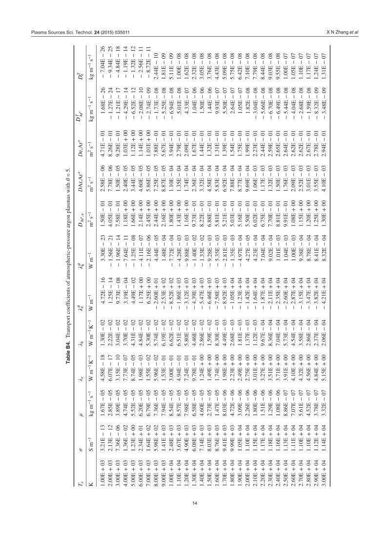
X N Zhang et al
14
Tab
le B
4. T
rans
port
coe
ffici
ents
of
atm
osph
eric
-pre
ssur
e ar
gon
plas
mas
with
θ =
5.
Te
σμ
λ eλ h
λθ eλθ h
+D
Ar
,eD
Ar,A
r+D
e,A
r++
DT A
rD
T e
KS
m−
1kg
m−
1 s−
1W
m−
1 K−
1W
m−
1 K−
1W
m−
1W
m−
1m
2 s−
1m
2 s−
1m
2 s−
1kg
m−
1 s−
1kg
m−
1 s−
1
1.00
E +
03
3.21
E −
13
1.67
E −
05
4.58
E −
18
1.30
E −
02
4.72
E −
16
3.30
E −
23
1.50
E −
01
2.58
E −
06
4.71
E −
01
1.68
E −
26
− 7
.04E
− 2
62.
00E
+ 0
32.
13E
− 1
22.
85E
− 0
56.
07E
− 1
72.
22E
− 0
21.
25E
− 1
4 −
1.5
6E −
21
4.05
E −
01
7.78
E −
06
8.26
E −
01
− 1
.27E
− 2
4 −
9.3
4E −
25
3.00
E +
03
7.36
E −
06
3.89
E −
05
3.15
E −
10
3.04
E −
02
9.73
E −
08
− 1
.96E
− 1
47.
58E
− 0
11.
50E
− 0
59.
28E
− 0
1 −
1.2
1E −
17
− 4
.84E
− 1
84.
00E
+ 0
31.
36E
− 0
24.
74E
− 0
57.
73E
− 0
73.
70E
− 0
23.
19E
− 0
4 −
7.6
4E −
11
1.18
E +
00
2.40
E −
05
1.03
E +
00
− 4
.29E
− 1
4 −
1.1
9E −
14
5.00
E +
03
1.23
E +
00
5.52
E −
05
8.74
E −
05
4.31
E −
02
4.49
E −
02
− 1
.25E
− 0
81.
66E
+ 0
03.
44E
− 0
51.
12E
+ 0
0 −
6.5
2E −
12
− 1
.32E
− 1
26.
00E
+ 0
32.
34E
+ 0
16.
20E
− 0
51.
98E
− 0
34.
84E
− 0
21.
17E
+ 0
0 −
4.1
1E −
07
2.14
E +
00
4.60
E −
05
1.14
E +
00
− 2
.08E
− 1
0 −
2.5
6E −
11
7.00
E +
03
1.64
E +
02
6.79
E −
05
1.55
E −
02
5.30
E −
02
6.25
E +
00
− 2
.16E
− 0
62.
45E
+ 0
05.
86E
− 0
51.
01E
+ 0
0 −
2.7
4E −
09
− 8
.72E
− 1
18.
00E
+ 0
35.
98E
+ 0
27.
36E
− 0
55.
96E
− 0
25.
74E
− 0
2 −
2.6
0E +
01
4.44
E −
05
2.44
E +
00
7.25
E −
05
7.88
E −
01
− 1
.73E
− 0
82.
44E
− 1
09.
00E
+ 0
31.
41E
+ 0
37.
94E
− 0
51.
53E
− 0
16.
19E
− 0
2 −
2.5
3E +
02
1.48
E −
04
2.16
E +
00
8.87
E −
05
5.67
E −
01
− 5
.25E
− 0
81.
81E
− 0
91.
00E
+ 0
42.
48E
+ 0
38.
54E
− 0
53.
00E
− 0
16.
62E
− 0
2 −
8.5
2E +
02
− 7
.72E
− 0
41.
80E
+ 0
01.
10E
− 0
43.
94E
− 0
1 −
6.9
4E −
08
5.11
E −
09
1.10
E +
04
3.67
E +
03
8.57
E −
05
4.94
E −
01
6.51
E −
02
− 1
.86E
+ 0
3 −
4.2
8E −
03
1.43
E +
00
1.35
E −
04
2.79
E −
01
5.01
E −
08
1.00
E −
08
1.20
E +
04
4.90
E +
03
7.98
E −
05
7.24
E −
01
5.80
E −
02
− 3
.12E
+ 0
3 −
9.8
8E −
03
1.16
E +
00
1.74
E −
04
2.09
E −
01
4.33
E −
07
1.62
E −
08
1.30
E +
04
6.08
E +
03
6.58
E −
05
9.78
E −
01
4.46
E −
02
− 4
.39E
+ 0
3 −
1.4
0E −
02
9.73
E −
01
2.36
E −
04
1.67
E −
01
1.04
E −
06
2.32
E −
08
1.40
E +
04
7.14
E +
03
4.60
E −
05
1.24
E +
00
2.86
E −
02
− 5
.47E
+ 0
3 −
1.3
3E −
02
8.22
E −
01
3.32
E −
04
1.44
E −
01
1.50
E −
06
3.05
E −
08
1.50
E +
04
8.03
E +
03
2.73
E −
05
1.49
E +
00
1.59
E −
02
− 6
.46E
+ 0
3 −
9.2
8E −
03
6.88
E −
01
4.58
E −
04
1.32
E −
01
1.44
E −
06
3.76
E −
08
1.60
E +
04
8.76
E +
03
1.47
E −
05
1.74
E +
00
8.30
E −
03
− 7
.58E
+ 0
3 −
5.3
5E −
03
5.81
E −
01
5.83
E −
04
1.31
E −
01
9.93
E −
07
4.43
E −
08
1.70
E +
04
9.41
E +
03
8.03
E −
06
1.98
E +
00
4.49
E −
03
− 8
.92E
+ 0
3 −
2.8
1E −
03
5.21
E −
01
6.92
E −
04
1.39
E −
01
5.50
E −
07
5.09
E −
08
1.80
E +
04
9.99
E +
03
4.72
E −
06
2.23
E +
00
2.68
E −
03
− 1
.05E
+ 0
4 −
1.3
5E −
03
5.03
E −
01
7.88
E −
04
1.54
E −
01
2.64
E −
07
5.75
E −
08
1.90
E +
04
1.05
E +
04
3.09
E −
06
2.49
E +
00
1.81
E −
03
− 1
.23E
+ 0
4 −
4.9
7E −
04
5.16
E −
01
8.77
E −
04
1.75
E −
01
1.05
E −
07
6.42
E −
08
2.00
E +
04
1.10
E +
04
2.26
E −
06
2.75
E +
00
1.37
E −
03
− 1
.42E
+ 0
44.
27E
− 0
55.
50E
− 0
19.
69E
− 0
41.
99E
− 0
11.
82E
− 0
87.
10E
− 0
82.
10E
+ 0
41.
15E
+ 0
41.
80E
− 0
63.
01E
+ 0
01.
12E
− 0
3 −
1.6
4E +
04
4.23
E −
04
6.02
E −
01
1.06
E −
03
2.23
E −
01
− 3
.04E
− 0
87.
79E
− 0
82.
20E
+ 0
41.
17E
+ 0
41.
51E
− 0
63.
27E
+ 0
09.
67E
− 0
4 −
1.8
7E +
04
7.04
E −
04
6.75
E −
01
1.17
E −
03
2.44
E −
01
− 5
.66E
− 0
88.
44E
− 0
82.
30E
+ 0
41.
18E
+ 0
41.
29E
− 0
63.
51E
+ 0
08.
36E
− 0
4 −
2.1
1E +
04
9.02
E −
04
7.70
E −
01
1.32
E −
03
2.59
E −
01
− 6
.70E
− 0
89.
03E
− 0
82.
40E
+ 0
41.
16E
+ 0
41.
08E
− 0
63.
71E
+ 0
07.
04E
− 0
4 −
2.3
5E +
04
1.01
E −
03
8.81
E −
01
1.50
E −
03
2.65
E −
01
− 6
.49E
− 0
89.
55E
− 0
82.
50E
+ 0
41.
13E
+ 0
48.
86E
− 0
73.
91E
+ 0
05.
73E
− 0
4 −
2.6
0E +
04
1.04
E −
03
9.91
E −
01
1.76
E −
03
2.64
E −
01
− 5
.44E
− 0
81.
00E
− 0
72.
60E
+ 0
41.
11E
+ 0
47.
07E
− 0
74.
10E
+ 0
04.
54E
− 0
4 −
2.8
7E +
04
1.00
E −
03
1.08
E +
00
2.09
E −
03
2.62
E −
01
− 4
.04E
− 0
81.
05E
− 0
72.
70E
+ 0
41.
10E
+ 0
45.
61E
− 0
74.
32E
+ 0
03.
58E
− 0
4 −
3.1
5E +
04
9.38
E −
04
1.15
E +
00
2.52
E −
03
2.62
E −
01
− 2
.68E
− 0
81.
10E
− 0
72.
80E
+ 0
41.
10E
+ 0
44.
52E
− 0
74.
56E
+ 0
02.
86E
− 0
4 −
3.4
7E +
04
8.78
E −
04
1.20
E +
00
3.01
E −
03
2.67
E −
01
− 1
.59E
− 0
81.
17E
− 0
72.
90E
+ 0
41.
12E
+ 0
43.
78E
− 0
74.
84E
+ 0
02.
37E
− 0
4 −
3.8
2E +
04
8.41
E −
04
1.25
E +
00
3.55
E −
03
2.78
E −
01
− 8
.32E
− 0
91.
24E
− 0
73.
00E
+ 0
41.
14E
+ 0
43.
32E
− 0
75.
15E
+ 0
02.
06E
− 0
4 −
4.2
1E +
04
8.32
E −
04
1.30
E +
00
4.10
E −
03
2.94
E −
01
− 3
.48E
− 0
91.
31E
− 0
7
Plasma Sources Sci. Technol. 24 (2015) 035011
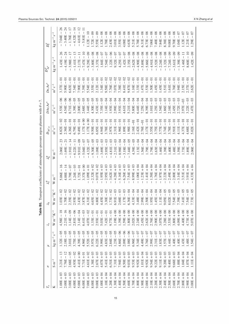
X N Zhang et al
15
Tab
le B
5. T
rans
port
coe
ffici
ents
of
atm
osph
eric
-pre
ssur
e ar
gon
plas
mas
with
θ =
7.
Te
σμ
λ eλ h
λθ eλθ h
+D
Ar
,eD
Ar,A
r+D
e,A
r++
DT A
rD
T e
KS
m−
1kg
m−
1 s−
1W
m−
1 K−
1W
m−
1 K−
1W
m−
1W
m−
1m
2 s−
1m
2 s−
1m
2 s−
1kg
m−
1 s−
1kg
m−
1 s−
1
1.00
E +
03
3.21
E −
13
1.32
E −
05
4.58
E −
18
1.03
E −
02
5.06
E −
16
2.06
E −
23
8.82
E −
02
1.53
E −
06
3.37
E −
01
1.43
E −
26
− 7
.04E
− 2
62.
00E
+ 0
37.
76E
− 1
22.
18E
− 0
52.
21E
− 1
61.
70E
− 0
24.
88E
− 1
4 −
1.6
9E −
21
2.36
E −
01
4.54
E −
06
5.90
E −
01
− 4
.19E
− 2
4 −
3.4
0E −
24
3.00
E +
03
2.68
E −
05
3.01
E −
05
1.14
E −
09
2.35
E −
02
3.79
E −
07
− 1
.91E
− 1
44.
36E
− 0
18.
71E
− 0
66.
63E
− 0
1 −
3.9
8E −
17
− 1
.76E
− 1
74.
00E
+ 0
34.
93E
− 0
23.
75E
− 0
52.
81E
− 0
62.
93E
− 0
21.
24E
− 0
3 −
6.2
2E −
11
6.79
E −
01
1.39
E −
05
7.34
E −
01
− 1
.41E
− 1
3 −
4.3
2E −
14
5.00
E +
03
4.41
E +
00
4.39
E −
05
3.14
E −
04
3.43
E −
02
1.72
E −
01
− 9
.91E
− 0
99.
49E
− 0
12.
00E
− 0
57.
90E
− 0
1 −
2.1
7E −
11
− 4
.61E
− 1
26.
00E
+ 0
37.
71E
+ 0
14.
96E
− 0
56.
41E
− 0
33.
87E
− 0
23.
37E
+ 0
0 −
5.0
4E −
07
1.17
E +
00
2.68
E −
05
7.39
E −
01
− 7
.47E
− 1
0 −
5.8
1E −
11
7.00
E +
03
4.61
E +
02
5.52
E −
05
4.07
E −
02
4.31
E −
02
− 1
.09E
+ 0
1 −
4.3
2E −
07
1.17
E +
00
3.44
E −
05
5.54
E −
01
− 9
.29E
− 0
91.
12E
− 1
08.
00E
+ 0
31.
38E
+ 0
35.
97E
− 0
51.
33E
− 0
14.
65E
− 0
2 −
2.3
2E +
02
− 9
.30E
− 0
59.
50E
− 0
14.
30E
− 0
53.
55E
− 0
1 −
3.8
0E −
08
1.72
E −
09
9.00
E +
03
2.67
E +
03
6.22
E −
05
2.93
E −
01
4.80
E −
02
− 9
.07E
+ 0
2 −
1.0
9E −
03
6.85
E −
01
5.43
E −
05
2.12
E −
01
− 3
.37E
− 0
85.
55E
− 0
91.
00E
+ 0
44.
07E
+ 0
35.
99E
− 0
55.
03E
− 0
14.
45E
− 0
2 −
1.9
5E +
03
− 3
.69E
− 0
34.
94E
− 0
17.
35E
− 0
51.
34E
− 0
11.
84E
− 0
71.
12E
− 0
81.
10E
+ 0
45.
41E
+ 0
34.
83E
− 0
57.
42E
− 0
13.
30E
− 0
2 −
2.9
5E +
03
− 5
.95E
− 0
33.
78E
− 0
11.
14E
− 0
49.
58E
− 0
27.
54E
− 0
71.
78E
− 0
81.
20E
+ 0
46.
51E
+ 0
32.
84E
− 0
59.
77E
− 0
11.
73E
− 0
2 −
3.6
2E +
03
− 4
.81E
− 0
32.
97E
− 0
11.
93E
− 0
47.
76E
− 0
21.
22E
− 0
62.
43E
− 0
81.
30E
+ 0
47.
31E
+ 0
31.
23E
− 0
51.
19E
+ 0
06.
91E
− 0
3 −
4.2
8E +
03
− 2
.31E
− 0
32.
31E
− 0
12.
99E
− 0
47.
07E
− 0
29.
32E
− 0
73.
01E
− 0
81.
40E
+ 0
47.
94E
+ 0
34.
86E
− 0
61.
39E
+ 0
02.
68E
− 0
3 −
5.1
6E +
03
− 8
.98E
− 0
41.
96E
− 0
13.
93E
− 0
47.
38E
− 0
24.
25E
− 0
73.
55E
− 0
81.
50E
+ 0
48.
50E
+ 0
32.
09E
− 0
61.
59E
+ 0
01.
17E
− 0
3 −
6.2
6E +
03
− 3
.18E
− 0
41.
89E
− 0
14.
61E
− 0
48.
41E
− 0
21.
42E
− 0
74.
08E
− 0
81.
60E
+ 0
49.
03E
+ 0
31.
08E
− 0
61.
80E
+ 0
06.
36E
− 0
4 −
7.5
4E +
03
− 7
.44E
− 0
51.
98E
− 0
15.
21E
− 0
49.
87E
− 0
22.
35E
− 0
84.
63E
− 0
81.
70E
+ 0
49.
53E
+ 0
36.
96E
− 0
72.
02E
+ 0
04.
33E
− 0
4 −
8.9
9E +
03
4.39
E −
05
2.16
E −
015.
80E
− 0
41.
16E
− 0
1 −
2.6
2E −
08
5.21
E −
08
1.80
E +
04
9.92
E +
03
5.34
E −
07
2.24
E +
00
3.48
E −
04
− 1
.06E
+ 0
41.
13E
− 0
42.
42E
− 0
16.
44E
− 0
41.
33E
− 0
1 −
4.9
0E −
08
5.78
E −
08
1.90
E +
04
1.01
E +
04
4.49
E −
07
2.45
E +
00
2.99
E −
04
− 1
.23E
+ 0
41.
56E
− 0
42.
76E
−01
7.25
E −
04
1.47
E −
01
− 5
.89E
− 0
86.
31E
− 0
82.
00E
+ 0
49.
92E
+ 0
33.
76E
− 0
72.
62E
+ 0
02.
50E
− 0
4 −
1.4
1E +
04
1.79
E −
04
3.17
E −
01
8.39
E −
04
1.53
E −
01
− 5
.86E
− 0
86.
73E
− 0
82.
10E
+ 0
49.
54E
+ 0
32.
99E
− 0
72.
76E
+ 0
01.
95E
− 0
4 −
1.5
8E +
04
1.79
E −
04
3.55
E −
01
1.01
E −
03
1.50
E −
01
− 4
.91E
− 0
87.
06E
− 0
82.
20E
+ 0
49.
22E
+ 0
32.
31E
− 0
72.
90E
+ 0
01.
45E
− 0
4 −
1.7
6E +
04
1.63
E −
04
3.75
E −
01
1.25
E −
03
1.45
E −
01
− 3
.52E
− 0
87.
40E
− 0
82.
30E
+ 0
49.
11E
+ 0
31.
83E
− 0
73.
07E
+ 0
01.
11E
− 0
4 −
1.9
7E +
04
1.46
E −
04
3.77
E −
01
1.54
E −
03
1.45
E −
01
− 2
.24E
− 0
87.
84E
− 0
82.
40E
+ 0
49.
20E
+ 0
31.
57E
− 0
73.
28E
+ 0
09.
05E
− 0
5 −
2.2
2E +
04
1.39
E −
04
3.74
E −
01
1.86
E −
03
1.51
E −
01
− 1
.32E
− 0
88.
38E
− 0
82.
50E
+ 0
49.
40E
+ 0
31.
44E
− 0
73.
53E
+ 0
08.
02E
− 0
5 −
2.4
9E +
04
1.40
E −
04
3.78
E −
01
2.16
E −
03
1.61
E −
01
− 7
.24E
− 0
99.
00E
− 0
82.
60E
+ 0
49.
68E
+ 0
31.
40E
− 0
73.
80E
+ 0
07.
54E
− 0
5 −
2.8
0E +
04
1.48
E −
04
3.91
E −
01
2.45
E −
03
1.76
E −
01
− 3
.61E
− 0
99.
70E
− 0
82.
70E
+ 0
41.
00E
+ 0
41.
40E
− 0
74.
09E
+ 0
07.
39E
− 0
5 −
3.1
4E +
04
1.59
E −
04
4.11
E −
01
2.72
E −
03
1.94
E −
01
− 1
.39E
− 0
91.
04E
− 0
72.
80E
+ 0
41.
04E
+ 0
41.
43E
− 0
74.
40E
+ 0
07.
41E
− 0
5 −
3.5
1E +
04
1.73
E −
04
4.37
E −
01
2.97
E −
032.
15E
− 0
1 −
1.4
6E −
11
1.12
E −
07
2.90
E +
04
1.07
E +
04
1.48
E −
07
4.73
E +
00
7.54
E −
05
− 3
.91E
+ 0
41.
89E
− 0
44.
68E
− 0
13.
22E
− 0
32.
37E
− 0
18.
60E
− 1
01.
21E
− 0
73.
00E
+ 0
41.
11E
+ 0
41.
54E
− 0
75.
07E
+ 0
07.
73E
− 0
5 −
4.3
3E +
04
2.06
E −
04
5.02
E −
01
3.47
E −
03
2.62
E −
01
1.42
E −
09
1.29
E −
07
Plasma Sources Sci. Technol. 24 (2015) 035011

X N Zhang et al
16
Tab
le B
6. T
rans
port
coe
ffici
ents
of
atm
osph
eric
-pre
ssur
e ar
gon
plas
mas
with
θ =
10.
Te
σμ
λ eλ h
λθ eλθ h
+D
Ar
,eD
Ar,A
r+D
e,A
r++
DT A
rD
T e
KS
m−
1kg
m−
1 s−
1W
m−
1 K−
1W
m-1
K-1
W m
−1
W m
−1
m2 s
-1m
2 s-1
m2 s
-1kg
m-1
s-1
kg m
-1 s
-1
1.00
E +
03
3.21
E −
13
1.05
E −
05
4.58
E −
18
8.16
E −
03
5.31
E −
16
1.22
E −
23
5.10
E −
02
8.80
E −
07
2.36
E −
01
1.21
E −
26
− 7
.04E
− 2
62.
00E
+ 0
31.
51E
− 1
21.
67E
− 0
54.
29E
− 1
71.
30E
− 0
29.
96E
− 1
5 −
3.0
7E −
23
1.35
E −
01
2.58
E −
06
4.13
E −
01
− 7
.35E
− 2
5 −
6.6
0E −
25
3.00
E +
03
5.20
E −
06
2.27
E −
05
2.22
E −
10
1.77
E −
02
7.73
E −
08
1.32
E −
16
2.47
E −
01
4.90
E −
06
4.64
E −
01
− 6
.98E
− 1
8 −
3.4
2E −
18
4.00
E +
03
9.59
E −
03
2.85
E −
05
5.46
E −
07
2.22
E −
02
2.53
E −
04
3.65
E −
12
3.81
E −
01
7.79
E −
06
5.14
E −
01
− 2
.46E
− 1
4 −
8.4
0E −
15
5.00
E +
03
8.70
E −
01
3.39
E −
05
6.19
E −
05
2.65
E −
02
3.59
E −
02
9.36
E −
10
5.34
E −
01
1.12
E −
05
5.61
E −
01
− 3
.74E
− 1
2 −
9.4
3E −
13
6.00
E +
03
1.69
E +
01
3.89
E −
05
1.43
E −
03
3.04
E −
02
9.67
E −
01
1.55
E −
08
6.88
E −
01
1.50
E −
05
5.83
E −
01
− 1
.21E
− 1
0 −
1.9
5E −
11
7.00
E +
03
1.24
E +
02
4.33
E −
05
1.19
E −
02
3.38
E −
02
7.02
E +
00
− 3
.20E
− 0
77.
87E
− 0
11.
93E
− 0
55.
39E
− 0
1 −
1.6
7E −
09
− 9
.47E
− 1
18.
00E
+ 0
34.
75E
+ 0
24.
73E
− 0
54.
87E
− 0
23.
69E
− 0
2 −
4.2
0E +
00
− 3
.53E
− 0
67.
79E
− 0
12.
40E
− 0
54.
43E
− 0
1 −
1.1
7E −
08
3.79
E −
11
9.00
E +
03
1.19
E +
03
5.09
E −
05
1.31
E −
01
3.97
E −
02
− 1
.68E
+ 0
2 −
6.5
5E −
05
6.94
E −
01
2.95
E −
05
3.40
E −
01
− 4
.27E
− 0
81.
15E
− 0
91.
00E
+ 0
42.
24E
+ 0
35.
40E
− 0
52.
72E
− 0
14.
19E
− 0
2 −
6.9
7E +
02
− 4
.34E
− 0
45.
87E
− 0
13.
63E
− 0
52.
54E
− 0
1 −
8.8
9E −
08
3.95
E −
09
1.10
E +
04
3.50
E +
03
5.49
E −
05
4.70
E −
01
4.19
E −
02
− 1
.69E
+ 0
3 −
1.3
9E −
03
4.93
E −
01
4.63
E −
05
1.92
E −
01
− 1
.02E
− 0
78.
67E
− 0
91.
20E
+ 0
44.
83E
+ 0
35.
23E
− 0
57.
14E
− 0
13.
84E
− 0
2 −
3.0
1E +
03
− 2
.81E
− 0
34.
26E
− 0
16.
38E
− 0
51.
54E
− 0
13.
79E
− 0
91.
51E
− 0
81.
30E
+ 0
46.
13E
+ 0
34.
43E
− 0
59.
86E
− 0
13.
04E
− 0
2 −
4.3
0E +
03
− 3
.82E
− 0
33.
80E
− 0
19.
66E
− 0
51.
33E
− 0
12.
79E
− 0
72.
27E
− 0
81.
40E
+ 0
47.
25E
+ 0
33.
14E
− 0
51.
26E
+ 0
01.
97E
− 0
2 −
5.3
9E +
03
− 3
.51E
− 0
33.
39E
− 0
11.
55E
− 0
41.
23E
− 0
15.
73E
− 0
73.
06E
− 0
81.
50E
+ 0
48.
16E
+ 0
31.
85E
− 0
51.
52E
+ 0
01.
08E
− 0
2 −
6.4
5E +
03
− 2
.35E
− 0
32.
90E
− 0
12.
37E
− 0
41.
18E
− 0
16.
09E
− 0
73.
80E
− 0
81.
60E
+ 0
48.
89E
+ 0
39.
82E
− 0
61.
77E
+ 0
05.
48E
− 0
3 −
7.6
7E +
03
− 1
.34E
− 0
32.
42E
− 0
13.
22E
− 0
41.
19E
− 0
14.
05E
− 0
74.
49E
− 0
81.
70E
+ 0
49.
53E
+ 0
35.
22E
− 0
62.
01E
+ 0
02.
86E
− 0
3 −
9.1
1E +
03
− 7
.28E
− 0
42.
10E
− 0
13.
95E
− 0
41.
28E
− 0
11.
86E
− 0
75.
15E
− 0
81.
80E
+ 0
41.
01E
+ 0
42.
96E
− 0
62.
26E
+ 0
01.
62E
− 0
3 −
1.0
8E +
04
− 4
.03E
− 0
41.
96E
− 0
14.
57E
− 0
41.
43E
− 0
14.
66E
− 0
85.
81E
− 0
81.
90E
+ 0
41.
07E
+ 0
41.
85E
− 0
62.
52E
+ 0
01.
02E
− 0
3 −
1.2
6E +
04
− 2
.28E
− 0
41.
94E
− 0
15.
16E
− 0
41.
62E
− 0
1 −
2.9
3E −
08
6.49
E −
08
2.00
E +
04
1.12
E +
04
1.27
E −
06
2.78
E +
00
7.07
E −
04
− 1
.47E
+ 0
4 −
1.2
9E −
04
2.01
E −
01
5.77
E −
04
1.84
E −
01
− 7
.03E
− 0
87.
18E
− 0
82.
10E
+ 0
41.
16E
+ 0
49.
38E
− 0
73.
05E
+ 0
05.
30E
− 0
4 −
1.7
0E +
04
− 6
.80E
− 0
52.
13E
− 0
16.
34E
− 0
42.
08E
− 0
1 −
9.2
1E −
08
7.88
E −
08
2.20
E +
04
1.19
E +
04
7.38
E −
07
3.31
E +
00
4.21
E −
04
− 1
.94E
+ 0
4 −
2.7
5E −
05
2.29
E −
01
6.98
E −
04
2.28
E −
01
− 1
.04E
− 0
78.
54E
− 0
82.
30E
+ 0
41.
19E
+ 0
45.
98E
− 0
73.
55E
+ 0
03.
43E
− 0
4 −
2.2
0E +
04
1.03
E −
06
2.47
E −
01
7.77
E −
04
2.44
E −
01
− 1
.07E
− 0
79.
14E
− 0
82.
40E
+ 0
41.
18E
+ 0
44.
87E
− 0
73.
76E
+ 0
02.
78E
− 0
4 −
2.4
6E +
04
2.15
E −
05
2.67
E −
01
8.78
E −
04
2.51
E −
01
− 1
.03E
− 0
79.
67E
− 0
82.
50E
+ 0
41.
15E
+ 0
43.
90E
− 0
73.
95E
+ 0
02.
20E
− 0
4 −
2.7
4E +
04
3.62
E −
05
2.82
E −
01
1.01
E −
03
2.52
E −
01
− 9
.19E
− 0
81.
01E
− 0
72.
60E
+ 0
41.
13E
+ 0
43.
07E
− 0
74.
15E
+ 0
01.
69E
− 0
4 −
3.0
3E +
04
4.69
E −
05
2.89
E −
01
1.18
E −
03
2.51
E −
01
− 7
.61E
− 0
81.
06E
− 0
72.
70E
+ 0
41.
11E
+ 0
42.
41E
− 0
74.
36E
+ 0
01.
28E
− 0
4 −
3.3
5E +
04
5.45
E −
05
2.88
E −
01
1.38
E −
03
2.52
E −
01
− 5
.88E
− 0
81.
11E
− 0
72.
80E
+ 0
41.
11E
+ 0
41.
93E
− 0
74.
60E
+ 0
09.
76E
− 0
5 −
3.7
0E +
04
5.96
E −
05
2.82
E −
01
1.61
E −
03
2.57
E −
01
− 4
.31E
− 0
81.
17E
− 0
72.
90E
+ 0
41.
13E
+ 0
41.
61E
− 0
74.
87E
+ 0
07.
67E
− 0
5 −
4.0
9E +
04
6.31
E −
05
2.76
E −
01
1.85
E −
03
2.67
E −
01
− 3
.05E
− 0
81.
24E
− 0
73.
00E
+ 0
41.
15E
+ 0
41.
43E
− 0
75.
18E
+ 0
06.
36E
− 0
5 −
4.5
1E +
04
6.61
E −
05
2.71
E −
01
2.09
E −
03
2.82
E −
01
− 2
.11E
− 0
81.
32E
− 0
7
Plasma Sources Sci. Technol. 24 (2015) 035011

X N Zhang et al
17
References
[1] Chapman S and Cowling T G 1970 The Mathematical Theory of Non-Uniform Gases 3rd edn (Cambridge: Cambridge University Press)
[2] Hirschfelder J O, Curtis C F and Bird R B 1964 Molecular Theory of Gases and Liquids 2nd edn (New York: Wiley)
[3] Devoto R S 1968 J. Plasma Phys. 2 617 [4] Murphy A B and Arundell C J 1994 Plasma Chem. Plasma
Process. 14 451 [5] Murphy A B 1995 Plasma Chem. Plasma Process. 15 279 [6] Capitelli M, Celiberto R, Gorse C and Giordano D 1995
Plasma Chem. Plasma Process. 16 267 [7] Murphy A B 2000 Plasma Chem. Plasma Process. 20 279 [8] Wang W, Rong M, Murphy A B, Wu Y, Spencer J W, Yan L D
and Fang M T 2011 J. Phys. D: Appl. Phys. 44 355207 [9] Murphy A B and Tam E 2014 J. Phys. D: Appl. Phys. 47 295202 [10] Yang G and Heberlein J V 2007 J. Phys. D: Appl. Phys. 40 5649 [11] Li H P, Heberlein J and Pfender E 2005 IEEE Trans. Plasma
Sci. 33 402 [12] Yang G and Heberlein J V 2007 Plasma Sources Sci. Technol.
16 529 [13] Devoto R S 1965 The transport properties of a partially
ionized monoatomic gas PhD Thesis Stanford University [14] Bonnefoi C 1983 Contribution to the study of methods to
solve the Boltzmann’s equation in a two-temperature plasma: example Ar–H2 mixture (in French) State Thesis University of Limoges, France
[15] Rat V, Aubreton J, Elchinger M F and Fauchais P 2001 Plasma Chem. Plasma Process. 21 355
[16] Rat V, Andre P, Aubreton J, Elchinger M F, Fauchais P and Lefort A 2001 Phys. Rev. E 64 026409
[17] Zhang X N, Li H P, Murphy A B and Xia W D 2013 Phys. Plasmas 20 033508
[18] Boulos M I, Fauchais P and Pfender E 1994 Thermal Plasmas: Fundamentals and Applications (New York: Springer)
[19] van de Sanden M C M, Schram P P J M, Peeters A G, van der Mullen J A M and Kroesen G M W 1989 Phys. Rev. A 40 5273
[20] Chen X and Han P 1999 J. Phys. D: Appl. Phys. 32 1711 [21] Prigogine I 1940 Bull. Cl. Sci. Acad. R. Belg. 26 53 [22] Potapov A V 1966 High Temp. 4 48 [23] Giordano D and Capitelli M 2001 Phys. Rev. E 65 16401 [24] Capitelli M, Colonna G and D’Angola A 2012 Fundamental
Aspects of Plasma Chemical Physics: Thermodynamics vol 66 (New York: Springer)
[25] Andre P, Aubreton J, Elchinger M F, Rat V, Fauchais P, Lefort A and Murphy A B 2004 Plasma Chem. Plasma Process. 24 435
[26] Griem H R 1962 Phys. Rev. 128 997 [27] Moore C E 1949 Atomic Energy Levels as Derived from the
Analyses of Optical Spectra vol 1 (Washington, DC: US National Bureau of Standards)
[28] Devoto R S 1973 Phys. Fluids 16 616 [29] Colombo V, Ghedini E and Sanibondi P 2008 Prog. Nucl.
Energy 50 921 [30] Aubreton A and Elchinger M F 2003 J. Phys. D: Appl. Phys.
36 1798 [31] Capitelli M, Bruno D and Laricchiuta A 2013 Fundamental
Aspects of Plasma Chemical Physics: Transport vol 74 (New York: Springer)
[32] Capitelli M, Celiberto R, Gorse C, Laricchiuta A, Minelli P and Pagano D 2002 Phys. Rev. E 66 016403
[33] Capitelli M et al 2012 Plasma Chem. Plasma Process. 32 427
[34] Rat V, Andre P, Aubreton J, Elchinger M F, Fauchais P and Vacher D 2002 J. Phys. D: Appl. Phys. 35 981
[35] Chen F F 2006 Introduction to Plasma Physics and Controlled Fusion vol 1 2nd edn (New Delhi: Springer) p 10
[36] Mitchner M and Kruger C H 1973 Partially Ionized Gases vol 8 (New York: Wiley) p 136
[37] Wang W Z, Rong M Z, Yan J D, Murphy A B and Spencer J W 2011 Phys. Plasmas 18 113502
[38] Rat V, Andre P, Aubreton J, Elchinger M F, Fauchais P and Lefort A 2002 Plasma Chem. Plasma Process. 22 475
[39] Chen X and Li H P 2003 Int. J. Heat Mass Transfer 46 1443 [40] Nemchinsky V 2005 J. Phys. D: Appl. Phys. 38 3825 [41] Li H P, Zhang X N and Xia W D 2013 Phys. Plasmas
20 033509
Plasma Sources Sci. Technol. 24 (2015) 035011