Embed Size (px)
Citation preview

at SciVerse ScienceDirect
Journal of Environmental Management 116 (2013) 36e49
Contents lists available
Journal of Environmental Management
journal homepage: www.elsevier .com/locate/ jenvman
Comparison of groundwater transit velocity estimates from flux theoryand water table recession based approaches for solute transport
Velu Rasiah*, John David Armour 1
Department of Environment and Resource Management, PO Box 156, Mareeba, QLD 4880, Australia
a r t i c l e i n f o
Article history:Received 19 May 2011Received in revised form14 November 2012Accepted 23 November 2012Available online 2 January 2013
Keywords:GroundwaterTransit velocityTransit timeWater table rise/recession ratesFlux theoryNitrate
* Corresponding author. Present address: School onology & Engineering, University of Ballarat, PO BAustralia. Tel.: þ61 7 4222 5449; fax: þ61 7 4222 549
E-mail addresses: [email protected] (derm.qld.gov.au (J.D. Armour).
1 Tel.: þ61 7 4048 4705; fax: þ61 7 4048 4759.
0301-4797/$ e see front matter � 2012 Elsevier Ltd.http://dx.doi.org/10.1016/j.jenvman.2012.11.025
a b s t r a c t
Reliable information in transit time (TT) derived from transit velocity (TV) for rain or irrigation water tomix with groundwater (GW) and the subsequent discharge to surface water bodies (SWB) is essential toaddress the issues associated with the transport of nutrients, particularly nitrate, from GW to SWB. Theobjectives of this study are to (i) compare the TV estimates obtained using flux theory-based (FT)approach with the water table rise/recession (WT) rate approach and (ii) explore the impact of thedifferences on solute transport from GW to SWB. The results from a study conducted during two rainyseasons in the northeast humid tropics of Queensland, Australia, showed the TV varied in space andover time and the variations depended on the estimation procedures. The lateral TV computed usingthe WT approach ranged from 1.00 � 10�3 to 2.82 � 10�1 m/d with a mean of 6.18 � 10�2 m/dcompared with 2.90 � 10�4 to 5.15 � 10�2 m/d for FT with a mean of 2.63 � 10�2 m/d. The vertical TVranged from 2.00 � 10�3 to 6.02 � 10�1 m/d with a mean of 1.28 � 10�1 m/d for the WT compared with6.76 � 10�3e1.78 m/d for the FT with a mean of 2.73 � 10�1 m/d. These differences are attributed to therole played by different flow pathways. The bypass flow pathway played a role only in WT but not in FT.Approximately 86e95% of the variability in lateral solute transport was accounted for by the lateral TVand the total recession between two consecutive major rainfall events. A comparison of TT from FT andWT approaches indicated the laterally transported nitrate from the GW to the nearby creek was rela-tively ‘new’, implying the opportunity for accumulation and to undergo biochemical reactions in GWwas low. The results indicated the WT approach produced more reliable TT estimates than FT in thepresence of bypass flow pathways.
� 2012 Elsevier Ltd. All rights reserved.
1. Introduction
Reliable information in transit time (TT), derived from transitvelocity (TV), for groundwater (GW) to travel to surface waterbodies (SWB) is essential to address the environmental healthissues associated with the transport of solutes, particularly nutri-ents, from GW to SWB. The TV/TT is the single fundamentaldescriptor that reveals information in GW storage, residence time,flow pathways, and the sources of water (McGuire and McDonnell,2006). These workers have also indicated the distribution of TTs inspace over time is equally important in situations where therewere‘loosing and gaining’ river situations and/or flip-flops occurred
f Science, Information Tech-ox 663, Ballarat, Vic 3350,3.V. Rasiah), john.armour@
All rights reserved.
simultaneously. Others have shown the TT for GW to travel fromaquifers to SWB will determine the opportunity for anthropogenicnutrients to undergo biogeochemical degradation (Burns et al.,2003; Scanlon et al., 2001) and consequently the loading in SWB.In summarising and discussing the merits and demerits of the TTestimates obtained using different approaches and models form 34published papers, McGuire and McDonnel (2006) reported thatthere were several unresolved issues that need attention.
The major issues cited by them are, how to account for thevariable flow in space over time, spatially varying transmissivity,discriminating vertical vs. lateral flows when they are coupled,immobile zones, and bypass flow at catchment scale. Acknowl-edging the aforementioned unresolved issues, the approaches thathave been used in past were based primarily on tracer/isotopecharacterisation along travel pathways (e.g. Maloszewski andZuber, 1982, 1993; Maloszewski et al., 1983; McGlynn et al., 2003;Uhlenbrook et al., 2003). Hoehn and Cirpka (2006) used watertemperature and tracers to assess the residence time of water inhypoheric GW in alluvial plains. Schneider et al. (2011) reported
V. Rasiah, J.D. Armour / Journal of Environmental Management 116 (2013) 36e49 37
that appropriate instrumentation techniques are also necessary toimprove the accuracies. Vogt et al. (2010) showed that electricalconductivity (EC), as a natural passive tracer, can be used for theestimation of TT for bank infiltration from a loosing stream atcatchment scale. In situations where catchment scale TTs arescarce, the logical step would be to gather experimental data for thecomputation of TT at least at transect scale that represent a land-scape unit.
In addressing the reliability of the transect scale TT estimatesobtained from flux theory-based (FT) equations Rasiah et al. (2011)reported the estimates ranged from6 yr to 69 yr to travel 650m andthe range depended on the subsurface saturated conductivity (Ks)used in the estimation equations which could spatially vary by anorder of magnitude, 0.72e8.64 m/d, over short distance (AustralianSoil Resource Information, 2001). Furthermore, the FT approachaccounts only for flow through soil matrix pathway (piston-flow)and disregards the flow through bypass flow pathways. In situa-tions where bypass flow pathways play a role the flow directionand velocity may vary temporally and these changes may have animpact on the TT estimates (De Vries and Simmers, 2002; Scanlonet al., 2001). These workers have also reported that if bypass flowpathways play any role in the recharge/discharge processes, theneven tracer results are questionable for recharge/discharge esti-mations. It seems there is a need to assess the TT estimates from FTagainst other approaches.
Healy and Cook (2002) had used the temporal changes in watertable levels for the estimation of TT for GW recharge anddischarges. This approach requires information only on specificyield and the changes in water table levels over time. The advan-tage of this approach includes not only its simplicity, but itsinsensitivity to the flow mechanisms and pathways. It seems this
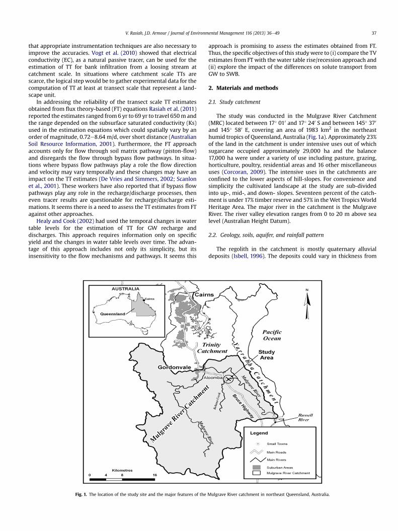
Fig. 1. The location of the study site and the major features of the
approach is promising to assess the estimates obtained from FT.Thus, the specific objectives of this studywere to (i) compare the TVestimates from FT with the water table rise/recession approach and(ii) explore the impact of the differences on solute transport fromGW to SWB.
2. Materials and methods
2.1. Study catchment
The study was conducted in the Mulgrave River Catchment(MRC) located between 17� 010 and 17� 240 S and between 145� 370
and 145� 580 E, covering an area of 1983 km2 in the northeasthumid tropics of Queensland, Australia (Fig.1a). Approximately 23%of the land in the catchment is under intensive uses out of whichsugarcane occupied approximately 29,000 ha and the balance17,000 ha were under a variety of use including pasture, grazing,horticulture, poultry, residential areas and 16 other miscellaneoususes (Corcoran, 2009). The intensive uses in the catchments areconfined to the lower aspects of hill-slopes. For convenience andsimplicity the cultivated landscape at the study are sub-dividedinto up-, mid-, and down- slopes. Seventeen percent of the catch-ment is under 17% timber reserve and 57% in theWet TropicsWorldHeritage Area. The major river in the catchment is the MulgraveRiver. The river valley elevation ranges from 0 to 20 m above sealevel (Australian Height Datum).
2.2. Geology, soils, aquifer, and rainfall pattern
The regolith in the catchment is mostly quaternary alluvialdeposits (Isbell, 1996). The deposits could vary in thickness from
Mulgrave River catchment in northeast Queensland, Australia.

V. Rasiah, J.D. Armour / Journal of Environmental Management 116 (2013) 36e4938
45 m to 100 m with coarse sands generally located between 15 mand 45 m below the surface. The regolith stratigraphy at 1 m depthincrements at the upslope location indicated that it ranged fromclay loam to fine sandy clay in the top 5 m and mottled claybetween 5 and 12 m depth (Fig. 2b and c). The latter suggestsprolonged saturation at depths greater than 5 m. The stratigraphyin the top 3 m at the midslope ranged from clay loam to silt, andgravelly sand, interbedded silty and clayey between 4 and10 m. Atdownslope the top 4 m was silty loam and underneath this layerwas a mix of gravel and sand. The lateral stratification from up- todown- slope, ranged from clay, silt, and sandmix to gravel and sandmix. It seems the alluvial depositions varied both laterally andvertically in the regolith. The majority of soils under sugarcane inMRC, including that at the experimental site, are alluvial acidicdrystrophic brown Dermosols (Orthic Tenosols) characterised by43e44% clay, 30e32% silt, and 23e24% sand in the top 0.20 m(Isbell, 1996; Murtha et al., 1996).
Fig. 2. The location of the wells along the transect (a), elevation and well depth (b
The aquifers in the humid tropics are recharged primarily by therainfall received during the summer rainy season, January to May(Hair, 1990; Rasiah et al., 2005, 2011). The depth to groundwater(GW) at the upslope ranged from 1 to 5 m from ground surfaceduring the rainy season and between>5m and<9mduring the dryseason, July toDecember (Rasiah et al., 2011). At downslope itwas atdepths less than 3m belowground surface throughout the year andthere may be positive heads during the rainy season (Rasiah et al.,2011). Published information in subsurface soil hydraulic proper-ties is scarce except that of Hair (1990). The long-term averagerainfall during the rainy season was 1600 mm with an annualaverage of 2200 mm (Rasiah et al., 2011). Rainfall during the inves-tigation period was recorded in an automated weather stationlocated at the study site and reported in Table 1. The average annualrunoff, deep drainage, and evapotranspiration, computed usingthree years of data, for the same catchment has been reported as610mm, 605mm, and 1117mm, respectively (Thorburn et al., 2010).
), and the regolith stratigraphy (c). The scale for Fig. 2a is w 0.01 m for 80 m.

Table 1Monthly rainfall distribution during the rainy seasons of 2007, 2008, and 2009 at the study site.
January(mm/month)
February(mm/month)
March(mm/month)
April(mm/month)
May(mm/month)
June(mm/month)
Total(mm)
Experimental site2007 279 1084 306 180 181 60 20962008 486 669 1076 38 74 37 23862009 933 883 218 187 107 14 2342Average 566 879 533 135 121 37 2271Coefficient of variation (%) 59 24 89 62 45 62
V. Rasiah, J.D. Armour / Journal of Environmental Management 116 (2013) 36e49 39
2.3. Piezometer installation and groundwater monitoring
Water table measurements and water sample collections werecarried out from six piezometers, hereafter referred to as wells,installed along a 650 m long transect that traversed througha typical undulating landscape in the catchment. For convenienceand simplicity the undulating topography of the landscape at thestudy site was sub-divided into up- mid- and down- slopes. Thetransect ran perpendicular to one of the Mulgrave River’s majortributaries, the Behana Creek. The location of the wells along thetransect, the elevation of the wells in Australian height datum(AHD), and the regolith profile characteristics are shown in Fig. 2aand b. Two wells were installed at a given slope position, up- ormid- or down- slope, along the transect and these two wells areconsidered as nested. At a given slope position, the 10 m or 12 mwell is referred to as the deep well and the 6 mwell as shallow andthey were w1.5 m apart. The deep wells 1b, 2a, and 3a were at up-mid- and down- slope positions, respectively, and 1c, 2b, and 3b,respectively, were the corresponding shallow wells (Fig. 2a). Theup- and mid- slope positions wells were z370 m apart and themid- and down- slope wells z 280 m apart. The AHD of the up-mid- and down- slope was 12.5 m, 9.0, and 6.5 m, respectively.
At each slope position two boreholes (96 mm diameter) thatwere 6 m and 10 or 12 m deep were drilled using a rotary mud rig.After drilling, PVC pipes (43 mm internal diameter) with tightlysealed base were inserted into the boreholes. Prior to insertion thebottom 3 m segments of pipes were slotted which were <1 mm by4e5 mm. The slotted segments were wrapped with 250 mmseamless polyester filter socks to prevent coarse sand entry into thewells but allowed water inflow. The space between the slottedsegments and the regolith wall was back-filled with coarse sandand a bentonite collar was placed just above the slotted segment ofthe pipe to prevent water entry from above. The space between thepipe and the profile above the collar was tightly back-filled withgrout and soil material up to the ground surface.
Water table measurements and sampling from the 6 wells wereconducted during the 2007 and 2009 rainy seasons at irregularintervals ranging from 7 to 12 days. During the 2008 season thewells were used for another other study. Groundwater monitoringand sampling were scheduled to occur 1e2 days after major rainfallevents and after dry-spells that lasted for at least 5e10 days. Theformer was used to infer information on water table risecharacteristics and the latter on recession. The water table wasmeasured using a tape with a noise device trigger attached to itand the samples for the chemical analysis were collected, afterwater table measurements, following the procedures describedby Alexander (2000). The samples were kept at approximately4 �C until arrival in the laboratory where they were frozen andanalysed for electrical conductivity (EC), nitrateeN, and chloride(Cl) following the procedures described by Rayment and Higginson(1992) in a laboratory accredited by the National Association ofTesting Authorities (Australia). The EC determination was con-ducted on all the collected samples but chloride and nitrate
determinations were carried out only on the samples collectedfrom wells-1b and 3b due to financial constraints.
2.4. Cropping and fertilizer history at the site
The experimental sitewas under native rainforest before clearedin early 1940’s and has been under sugarcane cultivation until now.Before the mid 1980’s the trash after was burned in situ and thischanged to a green-blanket system (all trash left on in situ beforeand after harvest) in 1990. Fertiliser-N input at the site during thestudy period ranged from 136 to 148 kg N/ha yr as urea and/ordiammonium phosphate. Fertiliser-N was split applied, once atplanting or for the ratoon crop (the crop that establishes itself fromrhizomes after harvest) in JuneeAugust and the second dressing inDecember, before the onset of the rainy season.
2.5. Transit velocity (TV), transit time (TT) and solute mass fluxes
In this study, matrix flow is defined as the flow through bulk soilinvolving piston-flow mechanism. The flow is slow, the velocitysame at any cross-section, the flow may occur under saturated orunsaturated condition, and the flow pathways is called matrix flowpathway. The bypass flow on the other hand is defined as unevenflow with varying velocities within and at different cross-sections,the flow is relatively fast and it occurs through cracks and crevices,root and worm channels, and soil-pipes (These definitions aresummarised from Google search).
The flux theory (FT) is applicable to only to piston-flow processand in this approach the TV through a unit cross-sectional area ofsoil matrix was computed using the following equation (Fetter,1999);
TV ¼ ðKs=hÞ*HG (1)
In Eq. (1) HG was the hydraulic gradient between 2 wells whichwas defined as;
HG ¼ ðH1 � H2Þ=l (2)
In Eq. (2), H1 and H2 were hydraulic heads in two wells, whereH1 > H2, and lwas the shortest distance between the wells. The HHare relative to the Australian height datum. The Ks in Eq. (1) wassaturated hydraulic conductivity and hwas effective porosity whichwe assumed as 0.15 (Rasiah et al., 2003) and the Ks as 0.6 m/d (unpublished pump test data from this study). The pump test wasconducted during the dry season (2008 JulyeDecember) at theexperimental site in the deep wells (10 m or 12 m).
In the computation of vertical TV the H1 and H2 in Eq. (2) werehydraulic heads in the shallow and deep wells at a given slopeposition, respectively, on a given day and l was difference betweenthe well depths. The l in Eq. (2) for the lateral TV computation wasthe distance between the two slope positions (370m or 280m) and

V. Rasiah, J.D. Armour / Journal of Environmental Management 116 (2013) 36e4940
H1 and H2 were the hydraulic heads in the wells at the two slopepositions on a given day. The vertical and lateral TVs werecomputed using all the recorded water table levels in the 6 wells.
The solute mass flux (Fl) in one dimensionwas defined by Fetter(1999) as a function of its concentration (C in g/m3) and TV (TV inm/d);
Fl ¼ TVhC (3)
The h in Eq. (3) has already been defined and Fl is in g/m2 d.The temporally changed nitrate, Cl, and EC mass fluxes, both
vertical and lateral, were computed on limited number of samplesanalysed for the first two analytes and the EC in almost all thecollected samples. Thus for consistency the major emphasis onsolute mass fluxes is placed on EC which is based on the findings ofVogt et al. (2010).
In the water table rise/recession (WT) approach the rate ofwater table rise (V(rr)) in a given well was computed using theheight, measured from the bottom of the well, of water tablesmeasured 1e2 days before (h1) and 1e2 days after (h2) a significantrainfall event (usually > 10e15 mm/d) as follows;
VðrrÞ ¼ ðh1 � h2Þ=tx (4)
In Eq. (4) the h1 and h2 are in meters and tx in days between theh1 and h2 measurements.
The water table recession rates (V(rc)) from a given well wascomputed using the height (z1) of the water table measured aftera significant rainfall event and that measured 7e12 days after thesame rainfall event (z2) as follows;
V�rc� ¼ ðz1 � z2Þ=ty (5)
where z1 and z2 are in meters and ty in days between z1 and z2measurements.
For consistency and to avoid confusion, the vertical TVcomputed using the FT approach is abbreviated as V(fv) and thelateral TV as V(fl). The water table rise rate in the WT approach isabbreviated as V(rr) and the recession rate as V(rc). The V(rr) andV(rc) from the WT approach in this study are considered asequivalent to the V(fv) and V(fl), respectively, of the FT approach.The equivalency assumption is invoked on the fact that both V(rr)and V(fv) represent recharges and the V(rc) and V(fl) the base-flowdischarges.
The aforementioned assumption has not been justified yet.Before we attempt to seek justifications we explore the reason(s)for the unusual observations reported by Rasiah et al. (2011), for thesame data as that is in this paper, with regards to the simultaneouswater table rises/recessions that occurred in the nested wells aswell as and along the transect, respectively. It should be noted theauthors didn’t provide any reason(s) for that unusual observationsin that paper. However, intuitively and logically it is usually ex-pected that when the water table recedes in the shallow nestedwell at a given slope position that the deep well will rise. Similarlywhen the water table recede, with limited or no vertical recharge,at the upslope position that the lower aspects to rise. Thus, for thesimultaneous rises/recessions that occurred and reported in theprevious paper, now we hypothesise in this study the followingscenarios. The simultaneous rises in water tables in the nestedshallow well after rainfall (RF) mostly to RF and that in the deepwell to subsurface lateral flow from hill-slopes above the croppedarea. In situations where the recharge is mostly by subsurfacelateral flow from hill-slope then the rate of rise may increase ordecrease with decreasing elevation. Furthermore, the rechargealong the transect could also be attributed to infiltration of surface
runoff from hill-slope and to creek intrusion, i.e. ‘loosing creek’situation, particularly at lower slope aspect (see introductionsection). The simultaneous recession along the transect could beattributed to drop in elevation (w12 m drop in elevation) associ-ated subsurface gravity flow, decreasing lateral gradients, anda ‘gaining creek’ situation (see the introduction). For the watertables not to rise at lower aspects while that at upslope recedescould be attributed to an increase in subsurface flow rate at loweraspects and/or a ‘gaining creek’ situation. Such conditions couldmash water table rises at lower aspects while the upslope looseswater. Thus, we will employ the aforementioned scenarios toprovide justification for the equivalency assumption and determinewhich TV estimation procedure provides the most appropriatejustification.
2.6. Statistical analysis
The temporal variations in depth to water tables, hydraulicheads, solute concentrations, V(fv), V(fl), V(rr), V(rc), and verticaland lateral solute fluxes are characterised using the descriptivestatistical parameters the mean, minimum, maximum, and thecoefficient of variation (CV). The characterisation approach is basedon that of von Asmuth and Knotters (2004) findings. Simple linearcorrelations were performed to determine the positive or negativeimpact of a given variable on the other. The SAS (1991) softwarepackage was used for the statistical analysis of data.
3. Results
3.1. Water table levels and hydraulic heads
The data shown in Fig. 3 for the shallow (6 m) and deep (10e12 m) wells along the transect indicate the depth to water table(DWT) and hydraulic head (HH) varied spatiotemporally. The DWTbegan to rise early in January with the onset of rains, fluctuatedduring mid January through April, and rapidly receded duringMayeJune to pre-January levels. The DWT variations at the upslopeshallow well ranged from 0.28 m to 5.53 m during rainy seasonscompared with 0.15 me5.11 m, and 0.34 me2.89 m, respectively,for the shallow well at mid- and down- slope positions andsimilar trends were observed for the deep wells. The high CVs,ranging from 27% to 45%, statistically support the large variations(Table 2). A comparison of the means across the 3 shallow wellsindicates they are significantly different from each other anda similar trend was observed across the deep wells. The mean DWTin the shallow well at a given slope position was less than thecorresponding deep well.
The functional relationship between DWT and rainfall (RF)indicates that only 20e61% of the temporal changes werecontrolled by RF (Table 2). The R2 indicate the RF influenceincreased with increasing distance away from upslope towards thecreek (Fig. 2a and Table 2). The influence of RF on hydraulic head(HH) was identical to that obtained for DWT (Table 2). Even thoughthe HH was computed using well elevation as an input variablealong with DWT the identical response suggest that elevationdifferences had insignificant impact on the temporal changes inDWTor HH. The increasing influencewith increasing distance awayfrom upslope towards the creek might have been due to theimpacts of static and other dynamic variables. First, we havealready shown the decreasing elevation, a static variable, withincreasing distance away from upslope towards the creek hadinsignificant influence on DWT. Secondly, the thick clay layer,a static variable, at z5.5 m depth at upslope might have retardedthe rainwater percolation at depths >5.5 m and this led to lowresponse at this slope position than at other slope positions.

(f)
1/1
/2
00
7
1/5
/2
00
7
29
/8
/2
00
7
27
/1
2/2
00
7
25
/4
/2
00
8
23
/8
/2
00
8
21
/1
2/2
00
8
20
/4
/2
00
9
18
/8
/2
00
9
16
/1
2/2
00
9
0
100
200
300
400
500
600
700
Ra
in
fa
ll (m
m)
(a)
0.0
1.5
3.0
4.5
6.0
7.5
9.0D
ep
th
to
w
ater tab
le (m
)
Rainfall
Upslope deep well
Upslope shallow well
(b)
Rainfall
Midslope deep well
Midslope shallow well
(c)
0
100
200
300
400
500
600
700
Ra
in
fa
ll (m
m)
Rainfall
Downslope deep well
Downslope shallow well
(d)
0.0
2.0
4.0
6.0
8.0
10.0
12.0
14.0
1/1
/2
00
7
1/5
/2
00
7
29
/8
/2
00
7
27
/1
2/2
00
7
25
/4
/2
00
8
23
/8
/2
00
8
21
/1
2/2
00
8
20
/4
/2
00
9
18
/8
/2
00
9
16
/1
2/2
00
9
H
yd
rau
lic h
ead
(m
)
(e)
1/1
/2
00
7
1/5
/2
00
7
29
/8
/2
00
7
27
/1
2/2
00
7
25
/4
/2
00
8
23
/8
/2
00
8
21
/1
2/2
00
8
20
/4
/2
00
9
18
/8
/2
00
9
16
/1
2/2
00
9
Fig. 3. The impact of rainfall (the cumulative received between two consecutive monitoring dates) on water table levels (a, b and c) and hydraulic head (d, e and f) along thetransect.
V. Rasiah, J.D. Armour / Journal of Environmental Management 116 (2013) 36e49 41
However, if clay layer was a retardation variable then the responseat midslope should be less than at upslope because the clay layer atmidslope was at z1.5 m depth. Thirdly, the increasing subsurfacelateral flow, a dynamic variable, from hill- and up- slopes towardsthe creek might have interacted with the groundwater (GW), theinteraction influence increased with increasing distance away fromupslope towards the creek and indirectly led to increasing responseof DWT to RF. Fourthly, a ‘loosing creek’, the second dynamicvariable, interacting with GW might have indirectly influenced theresponse which increased with increasing distance away fromupslope towards the creek. Fifth, runoff, the third dynamic variable,from hill- and up- slopes might have slowed down between mid-and down- slope positions thereby increasing the infiltration andresponses of DWT to RF. Another dynamic variable, the RF distri-bution and/or evapotranspiration might have varied along the650 m transect and had an impact on DWT, but we believe thisimpact over 650 m distance was small to negligible. It seems theother 3 dynamic variables might have indirectly affected theresponses of DWT to RF. The CVs indicate the influence of RF onwater table fluctuations was higher in the shallow than deep well.The slopes of equations indicate that at least 20 mm of rainfall wasneeded to produce any significant change in DWT at the upslope.
The HH can be used as a guide to gather information in GW flowdirections and flow rates. The HH in the upslope shallow wellvaried temporally from 7.32 m to 12.57 m compared with 4.20 me
8.52 m, and 3.68 me6.23 m, for the mid- and down- slope shallow
wells, respectively, and similar trends were observed for the deepwells. The CVs for HH are generally less than the correspondingCVs for DWT, suggesting the temporal changes in water tablefluctuations can be characterised better by DWT than HH(Table 2). A comparison of the average HH across the 3 shallowwells indicates they are significantly different from each other anda similar trend was observed across the deep wells. The mean HHfor the shallow well at a given slope position was higher than thecorresponding deep well, except at the downslope, suggestingvertical discharge from the shallow to deep well (Table 2). Themeans for HH decreased with increasing distance away fromupslope towards the creek, suggesting the potential for HH inducedlateral flow from upslope towards the creek. The decreasingelevation from upslope towards the creek also suggests thepotential for gravity induced flow towards the creek.
3.2. Water table rise and recession rates
The temporal changes in net water table rise after a given RFevent and the net recession between two consecutive RF eventsshown in Fig. 4 indicate that there were 4e8 recharge events perrainy season and 11e14 discharge events. The rate of rise definedas V(rr), computed using Eq. (4) indicates that it varied spatio-temporally and depended on well depth (Table 3). Temporally theV(rr) for the upslope wells varied by w2 orders of magnitude withamean of 0.123m/d for the shallowwell and 0.154m/d for the deep

Table 2A summary of selected descriptive statistics for the depth to water table (DWT) andhydraulic head (HH).
Selected descriptive statistics
Wells Mean Minimumemaximum CV (%)
Depth to water table (m)Upslope deep 4.08 � 0.24 0.48e8.40 37 (46)Upslope shallow 3.65 � 0.18 0.28e5.53 37 (60)Midslope deep 3.36 � 0.13 0.61e5.93 27 (47)Midslope shallow 2.84 � 0.16 0.15e5.11 45 (63)Downslope deep 2.20 � 0.10 0.33e3.60 31 (46)Downslope shallow 1.73 � 0.08 0.34e2.89 34 (58)
Hydraulic head (m)Upslope deep 8.70 � 0.23 4.45e12.3 18 (46)Upslope shallow 9.15 � 0.17 7.32e12.57 14 (60)Midslope deep 6.59 � 0.13 4.20e8.52 13 (46)Midslope shallow 7.18 � 0.16 4.50e9.98 17 (63)Downslope deep 4.84 � 0.09 3.99e6.21 12 (45)Downslope shallow 4.82 � 0.16 3.68e6.23 12 (58)
Linear relationship between depth to water table and rainfall (RF) receivedbetween two consecutive monitoring dates
Wells Intercept (m) Slope (m/mm) R2
Upslope deep nsUpslope shallow 4.14 �3.34 � 10�3 (8.74 � 10�4) RF 0.20Midslope deep 3.70 �2.75 � 10�3 (5.99 � 10�4) RF 0.33Midslope shallow 3.58 �5.28 � 10�3 (5.82 � 10�4) RF 0.58Downslope deep 2.57 �2.59 � 10�3 (4.55 � 10�4) RF 0.44Downslope shallow 2.09 �3.05 � 10�3 (3.29 � 10�4) RF 0.61
Linear relationship between hydraulic head and rainfall (RF)Upslope shallow 8.67 3.25 � 10�3 (8.58 � 10�4) RF 0.20
The numbers following the means and slopes are standard errors and those withinparenthesis following the coefficient of variation (CV) are number of observations.The regression equations are significant at P< 0.05, R2 is coefficient of determinationand ‘ns’ denotes not significant at P < 0.05.
V. Rasiah, J.D. Armour / Journal of Environmental Management 116 (2013) 36e4942
well (Table 3). Similar large variations were observed at mid- anddown- slope positions and the variations are supported by CVs thatranged from 71 to124% (Table 3). The mean V(rr) for the shallowwell was usually less than the corresponding deep well, except atmidslope, but this trend is physically impossible as the transit time(TT) for rainwater to percolate to depths >6 m should be longerthan that for <6 m depth. Higher V(rr) for deep wells than shallowmight have been due to flow through bypass pathways while shortcutting or reducing the normal matrix mixing at depths <6 m.
Regardless of the well depths, the average V(rr) generallyincreased with increasing elevation or with increasing distanceaway from the creek towards upslope, except for a discrepancy atthe midslope. The increasing V(rr) with increasing elevationsuggests percolation increased in the same direction. If we acceptthis claim, then the influence of RF on HH or DWT should alsoincrease in that direction but it was not (Table 2). The increasingV(rr) with increasing distance away from the creekmight have beendue to a ‘loosing creek’ and/or the subsurface flow from hill- andup- slopes reducing the percolation and these flows led to increasesin V(rr) with increasing distance away from the creek.
The recession rate defined as V(rc), computed using Eq. (5)varied spatiotemporally and depended on well depth (Table 3).Even though both V(rc) and V(rr) varied temporally by 2 orders ofmagnitude, the means indicate the V(rr) was generally an ordermagnitude higher than the corresponding V(rc). The means forV(rc) indicate it was generally higher for shallow than deep well,except at downslope. The V(rc) for the shallowwells increased withincreasing elevation from down- to mid- slope, suggesting thatelevation induced discharges might have led to a ‘gaining creek’situation between RF events. Alternately, the decreasing V(rc) withincreasing elevation, for the deep wells, suggests ‘loosing creek’
situation. It seems the ‘gaining and loosing creek’ situations playedroles in GW flow rates and directions during the recession phaseand both situations existed simultaneously during the recessionphase.
The increasing V(rc) of shallow wells with increasing elevationcould also be attributed to vertical discharge into the correspondingnested deep well. However, there is no evidence to suggest thatthere was vertical discharge from shallow to deep well during therecession phase at the study site as the water table level in deepwells didn’t rise when that in the shallow receded at any givenpoint in time or along the transect. Instead thewater tables recededsimultaneously both in the shallow and deep wells at any givenpoint in time at a given slope position or along the transect. Thelatter situation is possible if and only there was continuous flowthrough a pathway without any break in pathway connectivity,indirectly suggesting bypass flow while short cutting the normalmixing process along the pathway. Such continuous connectivity ispossible only through subsurface channels or soil-pipes.
3.3. Flux theory-based velocities
The vertical hydraulic gradients (VHG), particularly the means,indicate vertical discharge from shallow to deep well but it variedalong the transect and over time (Table 4). The vertical flow velocity(V(fv)) computed using the VHG indicate that it varied spatiotem-porally by five fold to 2 orders of magnitude along the transect andthe large variations are supported by CVs that ranged from 39% to83% (Table 4). Temporally, the V(fv) at downslope varied byw5 foldcompared withz2 orders of magnitude each at mid- and up- slopepositions. The mean V(fv) generally increased with increasingelevation or the distance away from the creek, except at midslope,and this trend is similar to that observed for V(rr), however theV(fv) is generally and order of magnitude less than the corre-sponding V(rr).
The lateral hydraulic gradients (LHG) indicate the GW flowedfrom upslope towards the creek (Table 5). The LHG varied spatio-temporally and the mean gradient from mid- to down- slopeaquifer segment at depth <6 m was higher than that for >6 msegment. This suggests the aquifer segment at depth <6 mcontributed more towards the flow to the creek than from >6 msegment. The opposite tend observed for the LHG from up- to mid-slope suggests the flow towards midslope from upslope was higherfrom aquifer segments at depth>6m than from<6m segment. Thelateral flow velocities, V(fl), varied spatiotemporally by one to twoorders of magnitude (Table 5). The means indicate the GW flowedfaster from mid- to down- slope aquifer segment at depth <6 mthan from >6 m segment. An opposite trend was observed for theflow from up- to mid- slope. The means also indicate the GWflowed faster from mid- to down- slope than from up- to mid-slope.
Using the mean V(rc) we suggested that there was a ‘gainingcreek’ situation from shallow wells and a ‘loosing creek’ for deepwells, but the LHG and V(fl) generally indicate there as a ‘gainingcreek’ situation regardless of well depth from mid- to down- slope.In thematerials andmethods section, Section 2.5, we proposed thatV(rc) and V(fl) represent discharge/recession phase lateral flowrates. The V(fl) from the mid- to down- slope was approximatelyone-half of the V(rc) at midslope, suggesting the two approachesproduced different flow rates. The differences are attributed todifferences in flow pathways and flow mechanisms. The V(rc)estimates are independent of flowmechanism and accounts for theflow through matrix and bypass flow pathways (Healy and Cook,2002). The V(fl) on the other hand is based on piston-flow mech-anism and flow pathway is through the matrix and does notaccount for the flow through bypass pathways (Fetter, 1999).

(a)
-3.0
-2.0
-1.0
0.0
1.0
2.0
3.0
4.0
5.0
1/01
/200
7
1/04
/200
7
1/07
/200
7
1/10
/200
7
1/01
/200
8
1/04
/200
8
1/07
/200
8
1/10
/200
8
1/01
/200
9
1/04
/200
9
1/07
/200
9
Water table rise and recession depths at upslopeshallow well
(b)
1/01
/200
7
1/04
/200
7
1/07
/200
7
1/10
/200
7
1/01
/200
8
1/04
/200
8
1/07
/200
8
1/10
/200
8
1/01
/200
9
1/04
/200
9
1/07
/200
9
Water table rise and recession depths at upslopedeep well
(c)
-3.0
-2.0
-1.0
0.0
1.0
2.0
3.0
4.0
5.0
1/01
/200
7
1/04
/200
7
1/07
/200
7
1/10
/200
7
1/01
/200
8
1/04
/200
8
1/07
/200
8
1/10
/200
8
1/01
/200
9
1/04
/200
9
1/07
/200
9
Re
ch
arg
e o
r d
isc
ha
rg
e (
m)
Water table rise and recession depths at midslopeshallow well
(d)
1/01
/200
7
1/04
/200
7
1/07
/200
7
1/10
/200
7
1/01
/200
8
1/04
/200
8
1/07
/200
8
1/10
/200
8
1/01
/200
9
1/04
/200
9
1/07
/200
9
Water table rise and recession depths at midslopedeep well
(e)
-3.0
-2.0
-1.0
0.0
1.0
2.0
3.0
4.0
5.0
1/01
/200
7
1/04
/200
7
1/07
/200
7
1/10
/200
7
1/01
/200
8
1/04
/200
8
1/07
/200
8
1/10
/200
8
1/01
/200
9
1/04
/200
9
1/07
/200
9
Water table rise and recession depths at downslopeshallow well
(f)
1/01
/200
7
1/04
/200
7
1/07
/200
7
1/10
/200
7
1/01
/200
8
1/04
/200
8
1/07
/200
8
1/10
/200
8
1/01
/200
9
1/04
/200
9
1/07
/200
9
Water table rise and recession depths atdownslope deep well
Fig. 4. The temporal changes in net water table rise and net recessions during the rainy seasons along the transect.
Table 3A summary of selected descriptive statistics for water table rise (V(rr)) and recessionrates (V(rc)).
Selected descriptive statistics
Wells Mean Minimumemaximum CV (%)
Rate of rise (m/d)Upslope deep 0.154 � 0.044 0.008e0.511 110 (15)Upslope shallow 0.123 � 0.025 0.002e0.325 84 (17)Midslope deep 0.102 � 0.030 0.004e0.494 124 (18)Midslope shallow 0.185 � 0.042 0.006e0.602 96 (18)Downslope deep 0.113 � 0.027 0.004e0.376 95 (16)Downslope shallow 0.093 � 0.018 0.002e0.224 71 (14)
Recession rate (m/d)Upslope deep 0.049 � 0.011 0.003e0.264 118 (28)Upslope shallow 0.052 � 0.009 0.004e0.254 106 (39)Midslope deep 0.064 � 0.010 0.013e0.170 77 (25)Midslope shallow 0.076 � 0.013 0.005e0.282 105 (39)Downslope deep 0.081 � 0.015 0.003e0.280 87 (24)Downslope shallow 0.049 � 0.009 0.001e0.159 105 (34)
The numbers following the means are standard errors and those within parenthesisfollowing the coefficient of variation (CV) are number of observations.
V. Rasiah, J.D. Armour / Journal of Environmental Management 116 (2013) 36e49 43
Furthermore, the V(fl) through any cross-section in a column orflow pathway should be same if not identical, but this condition isnot met at the study site, implying the flow, particularly was not100% matrix flow.
3.4. Solute concentrations and mass fluxes
Out of the six wells, the solute concentration data from themidslope deep well was disregarded due to a contamination issueduring well installation (Table 6). The CV, the maximum andminimum indicate that nitrate, EC, and Cl varied spatiotemporallyduring the rainy seasons and the variations are similar to DWTfluctuations (Table 6). For example the EC in the upslope deep wellranged from 3.20 � 10�2 dS/m to 1.34 � 10�1 dS/m, nitrate from23 mg/L to 1700 mg/L, and chloride from 3.66 � 103 mg/L to2.00 � 104 mg/L and similar trends were observed in the other 5wells (Table 5). The means indicate the EC in the deep well wasgenerally higher than the corresponding shallow well and a similartrend was observed for nitrate. The positive association between EC

Table 4A summary of selected descriptive statistics for vertical hydraulic gradient (VHG), vertical flow velocity, vertical solute fluxes and simple linear relationship between solutefluxes and VHG.
Selected descriptive statistics
Wells Mean Minimumemaximum CV (%)
Vertical hydraulic gradient (m/m)Upslope shallow to deep 1.85 � 10�2 � 3.13 � 10�3 1.67 � 10�3e8.33 � 10�2 83 (24)Midslope shallow to deep 1.76 � 10�1 � 2.47 � 10�2 2.50 � 10�2e4.38 � 10�1 67 (23)Downslope shallow to deep 7.22 � 10�3 � 6.67 � 10�4 2.50 � 10�3e1.50 � 10�2 39 (18)
Vertical flow velocity (m/d)Upslope shallow to deep 7.50 � 10�2 � 1.27 � 10�2 6.76 � 10�3e3.34 � 10�1 83Midslope shallow to deep 7.14 � 10�1 � 1.00 � 10�1 1.20 � 10�1e1.78 � 10�0 67Downslope shallow to deep 2.93 � 10�2 � 2.71 � 10�3 1.01 � 10�2e6.09 � 10�2 39
Ion fluxes (g/m2 d)Upslope shallow to deep 3.54 � 10�1 � 6.17 � 10�2 2.79 � 10�2e1.56 � 10�0 83 (24)Midslope shallow to deep 5.16 � 10�0 � 8.01 � 10�1 6.33 � 10�1e1.28 � 10þ1 72 (23)Downslope shallow to deep 1.06 � 10�0 � 3.16 � 10�1 4.68 � 10�2e5.56 � 10�0 165 (18)
NitrateeN flux (g/m2 d)Downslope shallow to deep 1.25 � 10�2 � 4.52 � 10�3 3.04 � 10�5e4.93 � 10�2 140 (15)
Chloride flux (g/m2 d)Downslope shallow to deep 4.32 � 10�1 � 1.26 � 10�2 1.15 � 10�2e1.14 � 10�0 97 (15)
Linear relationship between solute fluxes and VHG
Slope R2
Ion fluxUpslope shallow to deep 21.54 (0.86) VHG 1c_1b 0.94Midslope shallow to deep 32.50 (0.87) VHG 2b_2a 0.96Downslope shallow to deep 24.63 (0.15) VHG 3b_3a 0.99
Nitrate fluxDownslope deep to shallow 0.127(0.026) VHG 3b_3a 0.58
Chloride fluxDownslope shallow to deep 4.45 (0.21) VHG 3b_3a 0.97
The numbers following the means and slopes are standard errors and those within parenthesis following the coefficient of variation (CV) are number of observations. Theregression equations are significant at P< 0.05, R2 is coefficient of determination and ‘ns’ denotes not significant at P< 0.05. VHG 1c_1b refers to the vertical gradient from theshallow well 1c to the deep well 1b at the upslope position and similarly for the others.
Table 5A summary of selected descriptive statistics for lateral hydraulic gradient (LHG), lateral velocity, lateral solute fluxes and simple linear relationship between lateral ion fluxesand water table recession rates or LHG.
Selected descriptive statistics
Flux direction Mean Minimumemaximum CV (%)
Lateral hydraulic gradient (m/)Upslope deep to midslope deep 5.94 � 10�3 � 3.45 � 10�4 6.79 � 10�4e1.04 � 10�2 40 (45)Upslope shallow to midslope shallow 5.56 � 10�3 � 2.59 � 10�4 4.62 � 10�4e8.32 � 10�3 34 (54)Midslope deep to downslope deep 6.29 � 10�3 � 3.57 � 10�4 7.14 � 10�5e9.54 � 10�3 37 (43)Midslope shallow to downslope shallow 8.13 � 10�3 � 3.22 � 10�4 8.21 � 10�4e1.27 � 10�2 30 (56)
Lateral flow velocity (m/d)Upslope deep to midslope deep 2.41 � 10�2 � 1.40 � 10�3 2.70 � 10�3e4.25 � 10�2 39 (45)Upslope shallow to midslope shallow 2.26 � 10�2 � 1.05 � 10�3 1.88 � 10�3e3.38 � 10�2 34 (54)Midslope deep to downslope deep 2.56 � 10�2 � 1.45 � 10�3 2.90 � 10�4e3.87 � 10�2 37 (43)Midslope shallow to downslope shallow 3.30 � 10�2 � 1.31 � 10�3 3.33 � 10�3e5.15 � 10�2 30 (56)
Ion fluxes from Slope R2
Simple linear relationship between lateral ion fluxes and lateral gradient (LHG) or recession rate (V(rc)) or total recession (TR)Midslope deep to downslope deep 58.83 (2.59) LHG_10 0.88Midslope shallow to downslope shallow 28.72 (1.29) LHG_6 0.78Midslope deep to downslope deep 4.28 (0.62) V(rc)_10 0.71Midslope shallow to downslope shallow 1.92 (0.34) V(rc)_6 0.48Midslope deep to downslope deep 0.316 (0.044) TR_10 0.68Midslope shallow to downslope shallow 0.296 (0.047) TR_6 0.53
Ion fluxes as a function of LHG, TR, RR, and the interactions involving these variables.Midslope deep to downslope deep 48.11 LHG_10 þ 7.80 � 10�2 TR_10 0.95Midslope shallow to downslope shallow 28.71 LHG_6 þ 1.66 � 10�2 TR_6 0.86Nitrate flux from upslope deep to midslope 0.319 (0.054) LHG_10 0.60
The numbers following the means and slopes are standard error of estimates and those within parenthesis following the coefficient of variation (CV) are number of obser-vations. The correlations were significant at P< 0.05, and R2 is coefficient of determination. The LHG_10 refer to lateral gradient from the 10mwell and similarly for the others.TR_6 and TR_10 refer to total recession from the 6 m and 10 m wells, respectively.
V. Rasiah, J.D. Armour / Journal of Environmental Management 116 (2013) 36e4944
Table 6A summary of selected descriptive statistics for the selected solutes in groundwater.
Selected descriptive statistics
Wells Mean Minimumemaximum CV (%)
NitrateeN (m/L)Upslope deep 1012 � 81 23e1700 50 (40)Upslope shallow 945 � 85 800e1130 18 (4)Midslope shallow 1100 � 370 2e2200 75 (5)Downslope deep 892 � 290 70e1680 73 (5)Downslope shallow 364 � 52 2e1160 89 (39)
Electrical conductivity (dS/m)Upslope deep 8.08 � 10�2 � 2.90 � 10�3 3.20 � 10�2e1.34 � 10�1 23 (45)Upslope shallow 5.63 � 10�2 � 2.12 � 10�3 3.00 � 10�2e1.38 � 10�1 29 (60)Midslope shallow 7.40 � 10�2 � 2.34 � 10�3 4.40 � 10�2e1.61 � 10�1 25 (62)Downslope deep 6.20 � 10�2 � 1.25 � 10�3 4.80 � 10�2e9.00 � 10�2 14 (45)Downslope shallow 5.90 � 10�2 � 2.24 � 10�3 4.00 � 10�2e1.78 � 10�1 30 (60)
Chloride (m/L)Upslope deep 8.80 � 103 � 4.73 � 102 3.66 � 103e2.00 � 104 31 (32)Downslope shallow 7.17 � 103 � 2.56 � 102 2.04 � 103e8.52 � 103 20 (32)
r
Linear correlation between electrical conductivity (EC) and hydraulic head (HH) or nitrate or chlorideEC ¼ 8.86 � 10�3 HH (midslope shallow well) 0.85EC ¼ 1.10 � 10�2 HH (downslope shallow well) 0.97Nitrate ¼ 7013 � EC (Upslope deep well) 0.72Chloride ¼ 105,534 � EC (Upslope deep well) 0.93Nitrate ¼ 5320 � EC (Downslope shallow well) 0.76Chloride ¼ 105,534 � EC (Downslope shallow well) 0.95
The numbers following the means are standard errors and those within parenthesis following the coefficient of variations (CV) are number of observations. The correlationsare significant at P < 0.01 and r is correlation coefficient.
V. Rasiah, J.D. Armour / Journal of Environmental Management 116 (2013) 36e49 45
and nitrate or chloride suggest the constituents in total dissolvedsolutes (EC) changed with the changes in EC, implying that EC canbe used as a passive tracer to identify the transport directions of theconstituents, particularly nitrate, in the GW at the study site also(Vogt et al., 2010; Rein et al., 2009; Uchida et al., 2002).
Due to limited data for nitrate and chloride, we place theemphasis on ion fluxes (EC), both vertical and lateral (Tables 4 and5), based on the findings of Vogt et al. (2010). These workers haveused the temporal changes in EC to characterise solute flowdirection and pathways. As solute flux direction depends ongradients, we defined the temporal changes in vertical ion fluxes(EC) as a function of vertical hydraulic gradient (VHG), the lateralfluxes as a function of lateral hydraulic gradient (LHG), and theresults are summarised in Figs. 5 and 6, respectively. The regressionmodels for vertical ion fluxes indicate that 94%e99% of thetemporal changes are accounted for by VHG and the lateral fluxesby 78%e88% of the LHG (Table 4). Fifty eight percent of thevertical nitrate fluxes by VHG and 60% of the lateral fluxes by LHG.The regression models indicate the solutes were transportedvertically down and laterally towards the creek simultaneously. Themean TV indicated the vertical transport occurred faster thanlateral at least by 50% (Tables 4 and 5).
4. Discussion
4.1. Rainfall, water table level, and hydraulic head
We have shown that only 20%e61% of the temporal changes indepth towater table (DWT) or hydraulic head (HH) were controlledby rainfall, RF (Table 2). Visual inspection of the hydrograph shapesshown in Fig. 3 indicates the impact of RF on DWTor HH decreasedfrom up- to down- slope while the regression equations indicatejust an opposite trend. We proposed 6 suggestions in the Resultssection, 2 static and 4 dynamic variables, for the aforementioneddiscrepancy and showed only 3 dynamic variables might have hadindirect impact on the responses of DWT to RF. However, other
researchers (McGrath et al., 2010; Gu and Riley, 2009; Rein et al.,2009) have shown the temporal changes were controlled notonly by dynamic variables, but system variables such as elevation,well depth, and geology. Several other workers (Schneider et al.,2011; Vogt et al., 2010; Hoehn and Cirpka, 2006; Weiler et al.,2006; Uchida et al., 2002; Maloszewski and Zuber, 1993) haveshown the interaction between GW and creek/river flow hadsignificant impact on the temporal changes in DWT, GW flowdirection, flow volume in streams, and solute transport from GW tostreams.
Out of the aforementioned studies the results from Vogt et al.(2010) are more appropriate to our site than the others, as theprimary solute (EC) used in their study is also available for studysite. According to these workers the GW and river interaction attheir site was characterised by ‘loosing and gaining river’ situationsthat depended on RF events and the dry-spells that followed RFevents, respectively. They have also reported a flip-flop from‘loosing to gaining river’ situation led to significant temporalchanges in HH and EC in GW. The ‘gaining river’ was characterisedby pronounced diurnal variations in EC in GWand the ‘loosing river’by a high overall changes in EC after heavy RF events. We are not inpossession of the diurnal changes in EC but the overall changes inEC were high as indicated by CVs (Table 6). This indirectly suggeststhat there was an interaction between GW-creek water at our studysite. The correlations were significant only up to midslope from thecreek, implying the influence of the interaction extended only up tow280 m away from the creek (Table 6). Therefore, we suggest thehigher responses of DWTor HH up tow280 m away from the creekwere indirectly induced by the interaction between GW and thecreek. The overall higher responses of DWT or HH to RF plus theinteraction represents a ‘loosing creek’ situation and the low flow inthe creek during dry seasons (July to December) and between dry-spells between RF represent ‘gaining creek’ situation.
Another dynamic variable that we proposed was the subsurfaceand/or surface runoff flow from hill- or up- slopes interacting withthe GW at mid- down- slope positions. Other workers (Hencher,

Fig. 5. The impact of temporal changes in vertical hydraulic gradient on vertical ion fluxes along the transect.
V. Rasiah, J.D. Armour / Journal of Environmental Management 116 (2013) 36e4946
2010; Uchida et al., 2002) have shown the temporal changes wereimpacted by lateral bypass flow through soil-pipes, fissures andcrack, and root and worm channels. Uchida et al. (2002) have re-ported that lateral bypass flow through soil-pipes from hill-slope toa nearby river occurred after significant RF events (>70 mm), whileshort cutting the normal mixing processes in the soil matrix. Wesuggest a similar lateral bypass flow from upslope, while reducingthe normal mixing processes at the upslope, might have increasedthe response of DWT or HH with increasing distance away fromthe creek.
(a)
0.00
0.10
0.20
0.30
0.40
Ion
flu
x (
g/m
2
. d
)
Ion flux- upslope shallow well to midslope shallow
Lateral gradient- upslope shallow well to midslope shallow
(c)
0.00
0.20
0.40
0.60
0.80
1.00
25
/01
/07
25
/03
/07
25
/05
/07
25
/07
/07
25
/09
/07
25
/11
/07
25
/01
/08
25
/03
/08
25
/05
/08
25
/07
/08
25
/09
/08
25
/11
/08
25
/01
/09
25
/03
/09
25
/05
/09
Ion
flu
x (
g/m
2
. d
)
Ion flux- midslope shallow well to downslope shallow
Lateral gradient- midslope shallow well to downslope shallow
Fig. 6. The impact of temporal changes in lateral hyd
Namdar Ghanbari and Bravo (2011) indicated the temporalchanges in GW levels to significant RF events depended on themonitoring schedules followed suggesting the importance of thetiming of mentoring. According to these workers the temporalchanges were significant during the first 5 days after a significantRF event. The monitoring schedule followed, 1e2 days, aftera significant RF event at our study site probably captured the RFinduced maximum rise in GW levels. On the other hand the watertable levels recorded 7e12 days after a given RF event captured themaximum impact of dry spell between RF events on receding GW
(b)
0.000
0.003
0.006
0.009
0.012
Lateral h
yd
rau
lic g
rad
ien
t (
m/m
)
Ion flux- upslope deep well to midslope deep
Lateral gradient- upslope deep well to midslope deep
(d)
25
/01
/20
07
25
/03
/20
07
25
/05
/20
07
25
/07
/20
07
25
/09
/20
07
25
/11
/20
07
25
/01
/20
08
25
/03
/20
08
25
/05
/20
08
25
/07
/20
08
25
/09
/20
08
25
/11
/20
08
25
/01
/20
09
25
/03
/20
09
25
/05
/20
09
0.000
0.003
0.006
0.009
0.012
Lateral h
yd
rau
lic g
rad
ien
t (
m/m
)
Ion flux- midslope shallow well to downslope deep
Lateral gradient- midslope deep well to downslope deep
raulic gradient on ion fluxes along the transect.

V. Rasiah, J.D. Armour / Journal of Environmental Management 116 (2013) 36e49 47
levels. Thus, we suggest the monitoring schedule followed at ourstudy site was satisfactory to characterise the impact of RF on thetemporal changes in DWT or HH.
4.2. Transit velocity and transit time
The flux theory-based (FT) average vertical transit velocity(V(fv)), indicated the transit time (TT) for rainwater to recharge 1 mof the aquifer at the upslope position was w13 days (Table 4). Theaverage water table rise rate (V(rr)), from the water table (WT)approach, indicates the TT was w7 days (Table 3). The discrepancywas probably due to the differences in flow pathways as indicatedby De Vries and Simmers (2002). As indicated in the results section,the shorter TT from WT is attributed to the flow through bypasspathways compared with FT which doesn’t account for the bypassflow. The TT estimates from the WT approach are usually equal tothe observed water table rises; therefore we suggest the WTapproach is better than FT to produce reliable recharge TTestimatesin the presence of bypass flow pathways.
The FT based average lateral flow velocity (V(fl)) indicate the TTfor 1 m from the upslope shallow well towards the midslope wasw44 days compared with w19 days obtained using the averagerecession rate (V(rc)) of the WT approach (Table 3). The shorter TTfrom the WT approach was probably due to the role played by thelateral bypass flow pathways similar to that reported by Utchidaet al. (2002). These workers have reported that soil pipe-flowcontributed substantially towards the stream flow after the RFevents that were >70 mm. In our catchment RF events exceeding70 mm/d (Fig. 3) is a norm rather than an exception, suggesting thepotential for pipe-flow.
The TT estimates from the FT approach depends on theassumptions invoked in the computation of V(fl). In Eq. (2) the LHGwas considered to vary spatiotemporally whereas Ks and h wereassumed to be spatially invariant, but this assumption may not bevalid as they could also vary in space. The Ks in the north-easternhumid tropics had been shown to vary by an order of magnitude(0.61 m/d to 7.2 m/d, see the materials and methods section),suggesting the space invariant assumption invoked for the studysite may not be appropriate. Elsewhere in the text we indicatedthere was a general trend for V(fl) increase with increasing distanceaway from the creek. Hencher (2010) reported that even in uniformalluvial sand profiles the flow characteristics can be heterogeneousand may be space variant. Others (Gu and Riley, 2009; McGrathet al., 2010; Rein et al., 2009) have reported the characterisationof V(fl) and pollutant fluxes are “the most difficult, complex, anduncertain hydrological property to quantify”. Thus in the absence ofreliable information in spatially varying Ks and h, the V(fl) estimatesfrom the FT approach seem to be less reliable than that fromWT asthere is no need for the information in Ks and h in the latterapproach.
4.3. Transit time and solute transport to the creek
In situations where pollutant transport from GW to surfacewater bodies (SWB) is a major concern, reliable information in TTestimates is required to assess the hazard/risk associated withnutrient loading fromGW into sensitive aquatic ecosystems (Rasiahet al., 2005, 2010; Baker, 2003). The TT estimates obtained using themaximum V(fl) from the FT approach and the maximum the V(rc)from the WT approach indicated the TTs were w15 years and 2.7years, respectively, for the GW to travel w280 m from midslope tothe creek. Shorter TT implies insufficient opportunity for thenutrients to undergo biogeochemical and/or degradation/mineral-ization reactions under anaerobic conditions thereby increasing thepotentials for nutrient loading in SWB that receives GW discharges.
Weiler et al. (2006) indicated that in humid environment and withconducive soils, the subsurface stormwas an important contributortowards the flow volume in streams and solute transport.
We have shown that V(rc) played a substantial role in the TTestimates compared with V(fl). In order to clarify the relativeimportance of V(rc) vs V(fl) in relation to solute transport wedefined the lateral ion fluxes as a function of V(fl) or V(rc) and foundthat 48%e71% of the fluxes were controlled by the V(rc) comparedwith 78%e88% by V(fl) (Table 5). The regression models indirectlyindicate that lateral solute transport occurred through both matrixand bypass flow pathways and the influence of the former waslarger than the latter. However, if V(rc) had accounted for the flowthrough both matrix and bypass flow pathways (Healy and Cook,2002), then the R2 for ion fluxes defined by V(rc) should begreater than that defined by V(fl). Even though we are unable toprovide any reason as to why the control exerted by V(rc) is lessthan V(fl) we show the combined influence of matrix and bypassflow pathways was higher, R2 ¼ 86%e95%, than the individualinfluences. The latter statistically confirms that solute transport atthe study site occurred both through both matrix and bypass flowpathways.
Gu and Riley (2009) had reported that extrapolations from pointmeasurement of solute transport to catchment scale should takeinto consideration the issues of sorption and half-life of hydro-chemicals. Those with moderate sorption and long half-life aremost susceptible to transport within a year of application. They alsoreported that those with high potential for rapid transport showedlarge annual variability. The high CVs (Table 6) obtained in ourstudy show the solutes were transported relatively fast at the studysite and in this regard the role played by bypass flow pathways wassubstantial. Rein et al. (2009) reported, based entirely onmodelling,the extrapolation of point measurement of solute concentration forthe estimation for solute mass flux can only be undertakenprovided spatiotemporal variations in GW flow direction andvelocities are known. The results from this study while supportingtheir claim show how best to address the issue.
4.4. Assessment of the water table (WT) vs. flux theory-based (FT)transit velocity (TV) estimates
Based on the results from our study site we suggest the TVestimates from WT approach is more reliable than FT in situationswhere the bypass flow pathways play a major role in GW flow,particularly in laterally. However, Uchida et al. (2002) have re-ported that FT was satisfactory for their climatic condition. Thediscrepancy is therefore attributed to the heavy RF amounts andintensities, and thewell defined rainy vs. dry season encountered atour study compared with Uchida et al. (2002) study site. In climatessimilar to our study site and the bypass pathways playing a role inGW flow the impacts of ‘gaining or loosing’ river situations on TVestimates are better accounted by the WT than FT approach. Theapplicability of WT approach to account for the impact of head-water and large river on TV estimates are not known from ourstudy but the impacts are well documented for the FT approach(e.g. McGuire and Mc Donnell, 2006). Upscaling of TV from FTapproach to catchment scale has beenwell documented but that forWT is very limited (e.g. Healy and Cook, 2002). It seems 3e5measurement locations along a transect are satisfactory for theestimation of TV employing either approaches. Nested wells arenecessary for the estimation of both vertical and lateral TV alongsloping landscapes and our study shows 6e12 m deep wells aresufficient. The nested wells are needed to discriminate whichaquifer segment is receiving hill-slope flow and responding to RFand to identify which segment is ‘gaining or loosing’ water fromcreeks/rivers. Our study shows at least 2 seasons of data are needed

V. Rasiah, J.D. Armour / Journal of Environmental Management 116 (2013) 36e4948
to obtain reliable TV estimates provided the seasonal RF pattern issimilar to the long-term averages. Both approaches seem to besatisfactory to characterise the TVs of both post- and pre- RF events.The TV from FT depends largely on Ks which may vary spatially andfor such situations the WT approach seems to be more appropriatethan FT as WT is independent of Ks.
4.5. Hazard/risk of the nitrate in groundwater
We indicated the importance of the need for further knowledgeto address the hazard/risk issues associated with nutrient loadingfrom GW to surface waters, particularly to the Great Barrier Reef(GBR) lagoon (Baker, 2003). There are several unresolved issueswith regard to the fate of the nitrate in GW and its transport tosurface water bodies (SWB), particularly to the GBR. Of particularimportance with regard to the unresolved issues are thebiochemical reactions that may occur in soil and GW, the TT fromGW to SWB and the extent of dilution in SWB (Rasiah et al., 2011).Nevertheless, we propose to assess the hazard by comparing themedian nitrate against the ANZECC (2000) trigger values. Weconsider the median value as the most appropriate because theyrepresents 50% of the recorded observations. The trigger range forthe sustainable health of the GBR is 1e8 mg/L. The median nitrate inthe upslope deep well was 767 mg/L and that in the downslopeshallow well it was 248 mg/L. These values are 1e2 orders ofmagnitude higher than the trigger values proposed for thesustainable health of the GBR and for most of the other aquaticecosystems listed in ANZECC (2000) report for this region. Thus itseems the hazard associated with the nitrate in GW was high butthe risk depends on the unresolved issues listed above.
The rainfall total and the distribution pattern (Table 1) duringrainy seasons, high fertiliser-N input (50e60% out of 120 kg N/hatotal annual input) before the onset of rainy season, the green-blanket and the no-till systems of cultivation adopted for sugar-cane production, provide conditions favourable for the rapid trans-port of unused nitrate into shallow GW in this region (Rasiah et al.,2005; 2010). The high recession rates (Table 3) and lateral flowvelocities, V(fl), (Table 5) on the other hand suggest the GW andnitrate were transported to the creek were relatively fast, implyingthey are relatively ‘young’. Furthermore, the nitrate in GW undercropping in this region did not increase over the past 30e40 years(Armour et al., 2004) and the concentrations decreasing to the levels,after several spikes during rainy seasons, that existed before theonset of rainy season (Rasiah et al., 2005, 2010) indirectly suggeststhat there was little or no net accumulation in GW. This implies thenitrate in the GW was transported relatively fast to streams.
5. Conclusions
Using shallow groundwater (GW) fluctuation data in an alluvialaquifer in a humid tropical environment, transit velocities (TVs),particularly the lateral, were computed using flux theory-based(FT) and water table recession (WT) approaches to compare thetransit time ((TT) for water and solute transport fromGW to a creek.The mean lateral TV from the WT was approximately one-half ofthat from FT indicating the dependence of TV on estimationprocedures used. The differences are attributed to the additionalrole played by bypass flow pathways which are accounted for is inthe WT approach but not in FT. This indirectly suggests that WTapproach can be used to verify the presence or absence bypass flowpathways in regoliths and the role played by them in GW flow andTV. Furthermore, the WT approach is simple, doesn’t involvesophisticated chemical tracer use and analysis, implying the watertable rise/recession approach for TT estimates is cost effective. Theregression models indicated that lateral solute fluxes was
a function of the velocities from both approaches, indicating thetotal flow and the solute loads transported to streams from GW tosurface waters are characterised better collectively by bothapproaches rather than individually. The WT approach is appro-priate for high rainfall (RF) and high intensity climates charac-terised by well defined rainy and dry dry-spells between RF eventsand where bypass pathways play a role in GW flow and for ‘gainingand loosing’ river situations to produce more reliable TV than FT.The TV estimates from FT depends largely on Ks which may varyspatially and for such situations the WT approach is more appro-priate than FT as WT which is independent of Ks. A minimum of 3measurement locations along a landscape unit are necessary tocharacterise the variations in TV along landscape units and toidentify the hill-slope inflow and GW-creekwater interaction zoneswhich may have an impact on RF induced temporal changes in GWdynamics. For the aforementioned purposes at least 2 nested wellsinstalled at 6e10 m depths at a given location along the landscapeare needed to identify the aquifer segment receiving hill-slopeinflow, the responses of different aquifer segments to RF influ-ence, and to discriminate the impact of ‘gaining and loosing creeks/river’ situations on the dynamics of different aquifer segments.Minimum of 2 rainy seasons data are necessary to produce morereliable TV estimates than a single season which may differsubstantially from long-term RF pattern. The results indicate thereliability of TV estimates depend on the estimation procedureused, the incorporation of bypass flow, RF total and distribution,and the Ks values used.
Acknowledgements
The authors gratefully acknowledge the financial supportprovided by the Australian Research Council (Project numberLP06694390), the field and laboratory support provided byMr. D.H.Heiner, Ms. T. Whiteing, Mr. M. Dwyer, and Ms. D.E. Rowan, and theinternal review and editorial comments provided by Dr. C. Carrolland Ms. Glynis Orr.
References
Alexander, D.G., 2000. Hydrographic Procedure for Water Quality Sampling. WaterMonitoring Group, Water Resource Information & Systems Management.Department of Natural Resources, Brisbane, Australia.
ANZECC, ARMCANZ, 2000. Australian and New Zealand Guidelines for Fresh andMarine Water Quality 2000, No.4. National Water Quality ManagementStrategy. Australian and New Zealand Environment and Conservation Counciland Agriculture and Resource Management Council of Australia and NewZealand, Canberra.
Armour, J., Cogle, L., Rasiah, V., Russell, J., 2004. Sustaining the wet tropics:a regional plan for natural resource management. In: Condition Report:Sustainable Use, vol. 2B. Rainforest CRC and FNQ NRM Ltd, Cairns. Australia.
Australian Soil Resource Information, 2001. http://www.anra.gov.au/topics/soils/pubs/national/agriculture_asris_shc.html.
Baker, J., 2003. A Report on the Study of Land-sourced Pollutants and Their Impactson Water Quality in and Adjacent to the Great Barrier Reef. Department ofPrimary Industries, Brisbane, QLD, Australia.
Burns, D.A., Plummer, L.N., McDonnell, J.J., Busenberg, E., Casile, G.C., Kendall, C.,Hooper, R.P., Freer, J.E., Peter, N.E., Beven, K.J., Schlosser, P., 2003. Thegeochemical evolution of riparian groundwater in a forested piedmont catch-ment. Ground Water 41 (7), 913e925.
Corcoran, B., 2009. Mulgrave River Catchment. Terrain Natural Resource Manage-ment. http://www.terrain.org.au/our-region/areas/cairns/mulgrave.html.
De Vries, J.J., Simmers, I., 2002. Groundwater recharge: an overview of processesand challenges. Hydrogeology Journal 10 (1), 5e17.
Fetter, C.W., 1999. Contaminant Hydrogeology, second ed. Prentice Hall, ISBN0137512155.
Gu, C., Riley, R.J., 2009. Combined effects of short term rainfall patterns and soiltexture on soil nitrogen cycling e a modelling analysis. Journal of ContaminantHydrology 112, 141e154.
Hair, I.D., 1990. Hydrogeology of the Russell and Johnstone Rivers Alluvial Valleys,North Queensland. Department of Resource Industries, Brisbane, Australia.ISBN: 1034 7399.
Healy, R.W., Cook, P.G., 2002. Using groundwater levels to estimate recharge.Journal of Hydrology 10, 99e109.

V. Rasiah, J.D. Armour / Journal of Environmental Management 116 (2013) 36e49 49
Hencher, S.R., 2010. Preferential flow paths through soil and rock and their asso-ciation with landslides. Hydrological Processes 24, 1610e1630.
Hoehn, E., Cirpka, O.A., 2006. Assessing the residence times of hyporheic ground-water in two alluvial flood plains of the Southern Alps using water temperatureand tracers. Hydrology and Earth System Sciences 10, 553e563.
Isbell, R.F., 1996. The Australian Soil Classification. CSIRO, Melbourne, Australia.Maloszewski, P., Zuber, A., 1982. Determining the turn over time groundwater
systems with the aid of environmental tracers. 1. Models and their applicability.Journal of Hydrology 57, 207e231.
Maloszewski, P., Zuber, A., 1993. Principles and practice of calibration and validationof mathematical models for the interpretation of environmental tracer data.Advances in Water Resources 16, 173e190.
Maloszewski, P., Rauert, W., Stichler, W., Herrmann, A., 1983. Application of flowmodels in an alpine catchment area using tritium and deuterium data. Journalof Hydrology 66, 319e330.
McGlynn, B., McDonnell, J., Stewart, M., Seibert, J., 2003. On the relationshipbetween catchment scale and streamwater mean residence time. HydrologicalProcesses 17 (1), 175e181.
McGrath, G., Hinz, C., Sivapalan, M., 2010. Assessing the impact of regional rainfallvariability on rapid pesticide leaching potential. Journal of ContaminantHydrology 113 (1e4), 56e65.
McGuire, J.K., McDonnell, J.J., 2006. A review and evaluation of catchment transittime modelling. Journal of Hydrology 330, 543e563.
Murtha, G.G., Cannon, M.G., Smith, C.D., 1996. Soils of the Babinda-cairns Area,North Queensland. CSIRO Division of Soils, Divisional Report No. 123. CSIRO,Melbourne, Australia.
Namdar Ghanbari, R., Bravo, H.R., 2011. Evaluation of correlations betweenprecipitation, groundwater fluctuations, and lake level fluctuations usingspectral methods (Wisconsin, USA). Hydrogeology Journal 19 (4), 801e810.http://dx.doi.org/10.1007/s10040-011-0718-1.
Rasiah, V., Armour, J.D., Yamamoto, T., Mahendrarajah, S., Heiner, D.H., 2003. Nitratedynamics in shallow groundwater and the potential for transport to off-sitewater bodies. Water Air and Soil Pollution 147, 183e202.
Rasiah, V., Armour, J.D., Cogle, A.L., 2005. Assessment of the variables controllingnitrate dynamics in groundwater: Is it a threat to surface aquatic ecosystems?Marine Pollution Bulletin 51, 60e69.
Rasiah, V., Armour, J.D., Cogle, A.L., Florentine, S.K., 2010. Nitrate importeexportdynamics in groundwater interacting with surface-water in a wet-tropicalenvironment. Australian Journal of Soil Research 48, 361e370.
Rasiah, V., Armour, J.D., Nelson, P.N., 2011. Identifying the major variables control-ling the transport of water and analytes from an alluvial aquifer to streams.Journal of Environmental Hydrology 19. Paper 10.
Rayment, G.R., Higginson, F.R., 1992. Australian Laboratory Handbook of Soil andWater Chemical Method. Inkata Press, Sydney, Australia.
Rein, A., Bauer, S., Dietrich, P., Beyer, C., 2009. Influence of temporally variablegroundwater flow conditions on point measurements and contaminant massflux estimations. Journal of Contaminant Hydrology 108, 118e133.
SAS, 1991. SAS/STAT procedure guide for Personal Computers, Version 5. StatisticalAnalysis Systems Institute Inc., Cary, NC.
Scanlon, T.M., Raffensperger, J.P., Hornberger, G.M., 2001. Modelling transport ofdissolved silica in a forested headwater catchment: Implication for defining thehydrochemical response of observed flow pathways. Water Resources Research32 (12), 26e274.
Schneider, P., Vogt, T., Schimer, M., Doetsch, J., Linde, N., Pasquale, N., Perona, P.,Cirpka, O.A., 2011. Towards improved instrumentation for assessing river-groundwater interactions in a restored river corridor. Hydrological EarthSystem Sciences 15, 2531e2549.
Thorburn, P., Attard, S., Anderson, T., Davis, M., Kemei, J., Shanon, E., Milla, R.,Greiken, M.V., Davis, A, Brodie, J., 2010. Adopting Systems Approaches to Waterand Nutrient Management for Future Cane Production in the Burdekin. SRDCResearch Project CSE020, Final Report, ACFTR, Townsville, Australia.
Uchida, T.K., Kosugi, I., Mizuyama, T., 2002. Effects of pipe flow and bedrockgroundwater on runoff generation in a steep headwater catchment in Ashiu,central Japan. Water Resources Research 38 (7). http://dx.doi.org/10.1029/2001WR000261.
Uhlenbrook, S., Scissek, F., 2003. How to Estimate Mean Residence Time of Water ina Catchment? Results from a Model Comparison and Significance of IsotopeRecords. The General Assembly of the International Union of Geodesy andGeophysics (IUGG2003), Sapporo, Japan.
Vogt, T., Hoehn, E., Schneider, P., Freund, A., Schirmeer, M., Cirpka, O.A., 2010.Fluctuations of electrical conductivity as natural tracer for bank filtration ina losing stream. Advances in Water Resources 33, 1296e1308.
Von Asmuth, J.R., Knotters, M., 2004. Characterising groundwater dynamicsbased on a system identification approach. Journal of Hydrology 296,118e134.
Weiler, M., McDonnell, J.J., Tromp-van Meerveld, I., Uchida, T., 2006. Subsurfacestormflow. Encyclopedia of Hydrological Sciences. http://dx.doi.org/10.1002/0470848944.hsa.119.


![m b r a nce M e Journal of e o c l h a n r u ygol Membrane ... · [13]. At steady state the solute flux through the membrane is constant and equal to the solute flux throughout the](https://img.pdfslide.us/doc/110x75/5ebe30b0db125473e1434928/m-b-r-a-nce-m-e-journal-of-e-o-c-l-h-a-n-r-u-ygol-membrane-13-at-steady-state.jpg)