Comparison of Fracture Methodologies for Flaw Stability Analysis of Storage Tanks

This document was prepared in conjunction with work accomplished under Contract No.DE-AC09-96SR18500 with the U. S. Department of Energy.

DISCLAIMER

This report was prepared as an account of work sponsored by an agency of the United StatesGovernment. Neither the United States Government nor any agency thereof, nor any of theiremployees, makes any warranty, express or implied, or assumes any legal liability or responsibilityfor the accuracy, completeness, or usefulness of any information, apparatus, product or processdisclosed, or represents that its use would not infringe privately owned rights. Reference herein toany specific commercial product, process or service by trade name, trademark, manufacturer, orotherwise does not necessarily constitute or imply its endorsement, recommendation, or favoring bythe United States Government or any agency thereof. The views and opinions of authors expressedherein do not necessarily state or reflect those of the United States Government or any agencythereof.

This report has been reproduced directly from the best available copy.

Available for sale to the public, in paper, from: U.S. Department of Commerce, National TechnicalInformation Service, 5285 Port Royal Road, Springfield, VA 22161,phone: (800) 553-6847,fax: (703) 605-6900email: [email protected] ordering: http://www.ntis.gov/help/index.asp

Available electronically at http://www.osti.gov/bridgeAvailable for a processing fee to U.S. Department of Energy and its contractors, in paper, from: U.S.Department of Energy, Office of Scientific and Technical Information, P.O. Box 62, Oak Ridge, TN37831-0062,phone: (865)576-8401,fax: (865)576-5728email: [email protected]

http://www.ntis.gov/help/index.asp

http://www.osti.gov/bridge

mailto:[email protected]

mailto:[email protected]

WSRC-MS-2004-00209

1

COMPARISON OF FRACTURE METHODOLOGIES FOR FLAW STABILITY ANALYSIS OF STORAGE TANKS

P.-S. Lam and R. L. Sindelar Westinghouse Savannah River Company

Savannah River Technology Center Aiken, South Carolina

ABSTRACT Fracture mechanics methodologies for flaw stability

analysis of a storage tank were compared in terms of the maximum stable through-wall flaw sizes or “instability lengths.” The comparison was made at a full range of stress levels at a specific set of mechanical properties of A285 carbon steel and with a specific tank configuration. The two general methodologies, the J-integral-tearing modulus (J-T) and the failure assessment diagram (FAD), and several specific estimation schemes were evaluated. A finite element analysis of a flawed tank was also performed for validating the J estimation scheme with a curvature correction and for constructing the finite element-based FAD. The calculated instability crack lengths show that the J-T methodology based on a center-cracked panel solution with a curvature correction, and the material-specific FAD, most closely approximate the result calculated with finite element analysis for the stresses at the highest fill levels in the storage tanks (less than 124 MPa or 18 ksi). The results from the other FAD methods show instability lengths less than the J-T results over this range. INTRODUCTION

A comprehensive review of fracture mechanics methods that are appropriate for the carbon steel storage tanks at the Savannah River Site (SRS) is provided. A comparison of these methods at a range of stress conditions at a specific set of mechanical properties for A285 steel is made in order to identify those fracture methodologies that provide for the maximum flaw stability lengths.

The SRS tanks are operated at temperatures above 21 °C (70°F) to avoid the potential for brittle fracture. Fill limits for these tanks were previously developed based on a limit load methodology to avoid crack instability leading to a large rupture. This paper applies the J-integral and FAD fracture methodologies to evaluate flaw stability for a postulated

through-wall axial crack in the Type I tanks, a specific type of storage tank.

A comparison of the J-integral-tearing modulus and several FAD methodologies recommended in the API-579 (American Petroleum Institute Fitness-for-Service, first edition, January 2000) [1] Level 3 analysis has been performed. The API assessments include (1) Method A: General FAD based on the CEGB (Central Electric Generating Board, U.K.) R6 (Assessment of the Integrity of Structures Containing Defects [2]) Option 1; (2) Method B: Material-specific FAD which is the CEGB R-6 Option 2 using the actual stress-strain curve of the material [3]; (3) Method C: J-based FAD utilizing the finite element fracture mechanics calculations (CEGB R-6 Option 3); and (4) Method D: Ductile tearing FAD with assessment points evaluated with an actual fracture resistance (J-R) curve [4]. The geometry of a through-wall axial flaw in the storage tank is used as a benchmark to illustrate the various fracture methodologies. Only a hoop stress loading is considered and no factors of safety are applied.

Using the finite element analysis to calculate J is the “best-estimate” method to determine the instability flaw size. However, it is labor-intensive to build finite element models for each flaw configuration in a structure. Therefore, estimation schemes are typically developed. The finite element analysis described in this paper was performed to validate the J estimation method that is based on a center-cracked panel (CCP) solution [5] with a curvature correction for the tank geometry [6,7]. The finite element result was also used to construct a failure assessment diagram following API 579 Level 3 Method C [1]. The instability crack lengths derived from these approaches were compared. The comparison is made within a range of fracture energies (e.g., JIC and J3mm) and applied stresses to ensure equivalency and to justify use of the FAD approach for flaw stability analysis.

WSRC-MS-2004-00209

2

MATERIAL PROPERTIES The E400 heat of A285 steel was chosen for the material

input to the analyses. The tensile tests in Reference 3 followed the American Society for Testing and Materials (ASTM) E8-99 “Standard Test Methods for Tension Testing of Metallic Materials.” The fracture testing [4] was based on ASTM E1820-99 “Standard Test Method for Measurement of Fracture Toughness.” The true stress-true strain curve along with the Ramberg-Osgood idealization is shown in Figure 1. The data are from tensile test specimen E400-31 [3] which was tested at 27 °C (80 °F) with tensile axis parallel to the plate rolling direction. The J-R curve in Figure 2 was obtained with a compact tension specimen E400-L1 [4] tested at 21 °C (70 °F). The notch was perpendicular to the rolling direction of the plate. The power law fit of the J-R curve can also be found in Figure 2. The Young’s modulus of the material is 207 GPa (30,000 ksi), the 0.2% yield stress is 249 MPa (36.1 ksi), and the Poisson’s ratio is 0.3. The J-R curve in Figure 2 provides JIC= 191 kJ/m2 (1093 in-lb/in2) and J3mm= 625 kJ/m2 (3567 in-lb/in2), where JIC is the J value at crack initiation and J3mm is the J value evaluated at 3 mm crack extension in the fracture testing.

J-INTEGRAL METHODOLOGY An overview of the J-integral methodology is described

below. An estimation method for evaluating J-integral in a curved structure is discussed. The residual stress (or other secondary stresses) can be included in a general estimation procedure. Flaw Stability

The fracture properties and J-R curves are normally determined by the testing methods described in the ASTM standards. The J-R curve represents the material resistance of ductile crack growth and the test data are typically fit with a power law expression: J = C(∆a)m (1) where C and m are curve fitting parameters (Fig. 2).

The tearing stability of the material is characterized by the tearing modulus (T) which is proportional to the slope of the J-R curve (dJ/da) and is defined as

dadJET 2

oσ=

where J is the value of J-integral, σo is the 0.2% yield stress, and E is the Young’s modulus. Instability flaw lengths are evaluated based on the loading conditions of the structural component and are determined by an elastic-plastic J-integral or J-T analysis. The crack growth (J ≥ JIC) is stable if T < TR, where TR is the tearing modulus of the material. The intersection point of the applied J-T curve and the material J-T curve will define the stable crack growth limit [8-10].

0

10,000

20,000

30,000

40,000

50,000

60,000

70,000

0 0.01 0.02 0.03 0.04 0.05 0.06 0.07 0.08

True Strain

True

Str

ess

(psi

)

Test data from extensometerRamberg-Osgood fit with typical Data points chosen for FEA input

Ramberg-Osgood:

α=3.2 n=5.0

εεo

= σσo

+ α σσo

n

E = 3x107 psi

Figure 1. True Stress-True Strain Curve of A285 E400

Steel

E400 L1

0

1000

2000

3000

4000

5000

6000

0 0.01 0.02 0.03 0.04 0.05 0.06 0.07 0.08 0.09 0.1 0.11 0.12 0.13 0.14 0.15 0.16 0.17 0.18

∆a (inch)

J DEF

(in-

lb/in

2 )

Jdef = 16534(∆a)0.7177

JIC = 1093 in-lb/in2

J3mm = 3567 in-lb/in2

∆a = 3 mm

Figure 2. J-R Curve of A285 E400 Steel

Cut-off for J-controlled Crack Growth

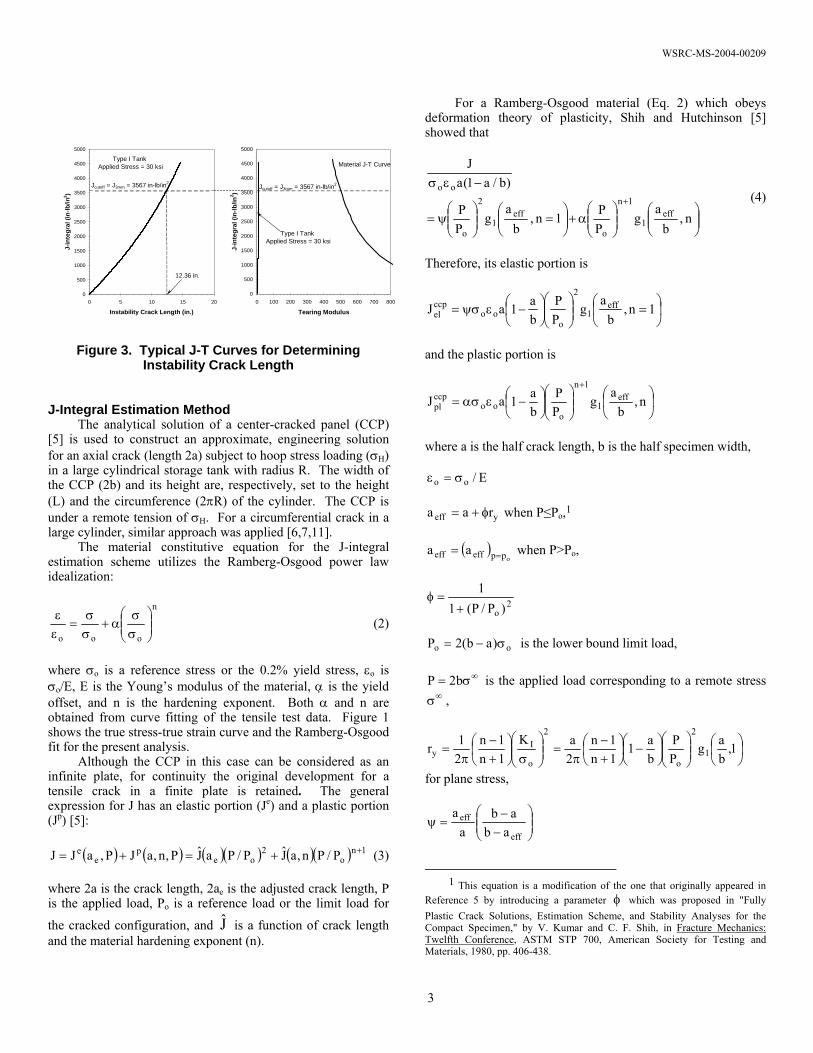
The designs of specimens for J-R fracture property testing ensure that a certain amount of stable crack growth can be obtained. Typically, the specimens do not generate data to the point where unstable crack growth begins. Therefore, extrapolation of the data could be made to determine the flaw instability. However, a conservative approach is to “cut-off” the material toughness data and to apply that cut-off value in the flaw stability analyses as shown in Figure 3 for a typical case of the storage tank. Under these circumstances, a cut-off J value at 3 mm crack extension [4] may be conservatively used (rather than extrapolating to a much higher J value) to determine the instability crack length. The design of the fracture testing specimen has allowed valid data up to approximately 3 mm extension in crack length [4]. The JIC (J at crack initiation) was also used as a very conservative cut-off value to estimate the instability crack length. In this case no credit was taken for the stable crack growth expected in ductile materials.

WSRC-MS-2004-00209

0

500

1000

1500

2000

2500

3000

3500

4000

4500

5000

0 100 200 300 400 500 600 700 800

Tearing Modulus

J-in

tegr

al (i

n-lb

/in2 )

Jcutoff = J3mm = 3567 in-lb/in2

Type I Tank Applied Stress = 30 ksi

Material J-T Curve

0

500

1000

1500

2000

2500

3000

3500

4000

4500

5000

0 5 10 15 20

Instability Crack Length (in.)

J-in

tegr

al (i

n-lb

/in2 )

Type I Tank Applied Stress = 30 ksi

Jcutoff = J3mm = 3567 in-lb/in2

12.36 in.

Figure 3. Typical J-T Curves for Determining

Instability Crack Length J-Integral Estimation Method

The analytical solution of a center-cracked panel (CCP) [5] is used to construct an approximate, engineering solution for an axial crack (length 2a) subject to hoop stress loading (σH) in a large cylindrical storage tank with radius R. The width of the CCP (2b) and its height are, respectively, set to the height (L) and the circumference (2πR) of the cylinder. The CCP is under a remote tension of σH. For a circumferential crack in a large cylinder, similar approach was applied [6,7,11].

The material constitutive equation for the J-integral estimation scheme utilizes the Ramberg-Osgood power law idealization:

n

ooo⎟⎟⎠

⎞⎜⎜⎝

⎛σσ

α+σσ

=εε (2)

where σo is a reference stress or the 0.2% yield stress, εo is σo/E, E is the Young’s modulus of the material, α is the yield offset, and n is the hardening exponent. Both α and n are obtained from curve fitting of the tensile test data. Figure 1 shows the true stress-true strain curve and the Ramberg-Osgood fit for the present analysis.

Although the CCP in this case can be considered as an infinite plate, for continuity the original development for a tensile crack in a finite plate is retained. The general expression for J has an elastic portion (Je) and a plastic portion (Jp) [5]:

( ) ( ) ( )( ) ( )( ) 1n

o2

oep

ee P/Pn,aJP/PaJP,n,aJP,aJJ ++=+= (3)

where 2a is the crack length, 2ae is the adjusted crack length, P is the applied load, Po is a reference load or the limit load for

the cracked configuration, and is a function of crack length and the material hardening exponent (n).

J

For a Ramberg-Osgood material (Eq. 2) which obeys deformation theory of plasticity, Shih and Hutchinson [5] showed that

⎟⎟⎠

⎞⎜⎜⎝

⎛⎟⎟⎠

⎞⎜⎜⎝

⎛α+⎟⎟

⎠

⎞⎜⎜⎝

⎛=⎟⎟

⎠

⎞⎜⎜⎝

⎛ψ=

−εσ+

n,b

ag

PP1n,

ba

gPP

)b/a1(aJ

eff1

1n

o

eff1

2

o

oo (4)

Therefore, its elastic portion is

⎟⎠

⎞⎜⎝

⎛ =⎟⎟⎠

⎞⎜⎜⎝

⎛⎟⎠⎞

⎜⎝⎛ −εψσ= 1n,

ba

gPP

ba1aJ eff

1

2

ooo

ccpel

and the plastic portion is

⎟⎠

⎞⎜⎝

⎛⎟⎟⎠

⎞⎜⎜⎝

⎛⎟⎠⎞

⎜⎝⎛ −εασ=

+

n,b

ag

PP

ba1aJ eff

1

1n

ooo

ccppl

where a is the half crack length, b is the half specimen width,

E/oo σ=ε

yeff raa φ+= when P≤Po,1

( )

oppeffeff aa == when P>Po,

2o )P/P(1

1+

=φ

oo )ab(2P σ−= is the lower bound limit load,

∞σ= b2P is the applied load corresponding to a remote stress

, ∞σ

⎟⎠⎞

⎜⎝⎛

⎟⎟⎠

⎞⎜⎜⎝

⎛⎟⎠⎞

⎜⎝⎛ −⎟

⎠⎞

⎜⎝⎛

+−

π=⎟⎟

⎠

⎞⎜⎜⎝

⎛σ

⎟⎠⎞

⎜⎝⎛

+−

π= 1,

bag

PP

ba1

1n1n

2aK

1n1n

21r 1

2

o

2

o

Iy

for plane stress,

⎟⎟⎠

⎞⎜⎜⎝

⎛−

−=ψ

eff

eff

abab

aa

1 This equation is a modification of the one that originally appeared in Reference 5 by introducing a parameter which was proposed in "Fully Plastic Crack Solutions, Estimation Scheme, and Stability Analyses for the Compact Specimen," by V. Kumar and C. F. Shih, in

φ

Fracture Mechanics: Twelfth Conference, ASTM STP 700, American Society for Testing and Materials, 1980, pp. 406-438.

3

WSRC-MS-2004-00209

and

232

1 ba044.0

ba37.0

ba5.011,

bag

⎥⎥⎦

⎤

⎢⎢⎣

⎡⎟⎠⎞

⎜⎝⎛−⎟

⎠⎞

⎜⎝⎛−−π=⎟

⎠⎞

⎜⎝⎛

For the A285 Grade B carbon steel, the tensile properties

were obtained from an E-400 heat specimen [3]. The Ramberg-Osgood exponent n is 5 and the yield offset α is 3.2 (Fig. 1). Therefore, the values for g1(a/b, n=5) can be calculated according to the procedure described in Reference 5:

a/b g1(a/b, n=5) 0 7.515

1/8 4.518 1/4 3.195 1/2 1.811 3/4 1.208 1 0.835

Curvature Corrections

A curvature correction is applied to estimate the J-integral values for the through-wall flaws in the sidewall of a tank. In the linear elastic fracture mechanics, the stress intensity factor (K) of a crack is usually expressed in a general form,

K Y a= σ π , where σ is the applied stress and Y is a function of crack size and specimen dimensions. In the linear elastic regime, J ∝ K2. The curvature correction factor, for estimating J-integral of a crack in a curved structure based on a corresponding infinite flat plate solution with the same crack length, is therefore Y2.

The curvature correction factors for a tank or a pipe can be obtained with handbook solutions, such as Reference 12 by Erdogen, and Reference 13 by Rooke and Cartwright. The solutions provided by Tada et al. [14] are simpler to use and the solutions are more representative in some cases. For an axial (longitudinal) crack, the solution in Reference 14 is used. The stress intensity factor of an axial crack with length 2a subjected to a hoop stress σH in a cylinder with mean radius R and thickness t is

)(YaK HI λπσ=

where Rta

=λ

225.11)(Y λ+=λ for 0<λ≤1, and

λ+=λ 9.06.0)(Y for 1≤λ≤5

In this case the curvature correction factor for the J-integral of an axial or a longitudinal crack is Y2, as noted earlier.

General Procedure for Combining J-integral Contributions

The J-integral is typically calculated with only the primary loads acting on the structural component.2 However, a procedure commonly used to readily combine the secondary stress and/or residual stress contributions to the J-integral was developed previously [6-8]. This procedure is summarized in the following: (1) For a given applied stress, calculate the CCP solution of

Shih and Hutchinson [5] for various crack lengths. The J-integral (Jccp) is composed of an elastic portion (Jel

ccp) and a plastic portion ( ), that is, . ccp

plJ ccppl

ccpel

ccp JJJ +=

(2) The plastic zone size correction (or small scale yielding correction) is applied to . ccp

elJ(3) The CCP solution is corrected for the curvature of the shell

or cylindrical structure. The approximated J-integral values for cracks in a tank ( and ) are

and , respectively.

curelJ cur

plJccpel

2curel JYJ = ccp

pl2cur

pl JYJ =

(4) The contributions of the stress intensity factor (K) from the other sources, such as the thermal stress or the residual stress, can be combined in the sense of linear elastic fracture mechanics. The elastic portion of J-integral ( )

in (3) above is first converted to , the Mode I stress intensity factor due to the applied load. Therefore,

curelJ

applIK

curel

applI EJK = under plane stress condition.

(5) Note that (stress intensity factor due to the residual

stress) is saturated to a maximum value ( ) when the crack is extended in length only a fraction of the plate thickness [15,16]. Therefore, the residual stress of this type is not subject to curvature correction. A series of numerical solutions for the stress intensity factors were obtained by simulating the welding process and taking into consideration the effect of residual stress redistribution as a result of crack growth [16-18].

resIK

resmaxK

(6) The total elastic portion of J is calculated as

( )2resmax

applI

e KKE1J +=

(7) The plastic portion of J remains unchanged, that is, curpl

p JJ =(8) Finally, the total J-integral at the crack tip is combined as

pe JJJ +=

It is noted that a similar combination scheme involving the conversion between the J-integral and the stress intensity factor (K) was adopted in API 579 (Section 9.4.3 of [1]). This conversion , such as those used in (4) and (6) above, is strictly 2 To calculate the J-integral accurately, a rigorous finite element analysis would be performed to simultaneously combine all the stresses including the residual stress. This is not done in practice due to the intensive modeling time required.

4

WSRC-MS-2004-00209

valid when the material is linear elastic. This has also been recognized by API 579 Appendix F.4.2.1 [1]: “For most materials and structures covered by this document, it is possible to measure toughness only in terms of J and CTOD; valid KIC data can only be obtained for brittle materials or thick sections.” The stress intensity factor at crack initiation, KIC, is commonly referred to the fracture toughness of the material. Under plane strain small scale yielding conditions, the equivalent fracture parameter converted from the J-R data is denoted by KJC. FINITE ELEMENT VALIDATION

The finite element method was used to assess the degree of validity of the CCP solution with curvature correction. In addition, the numerical results were used to construct failure assessment diagrams based on API 579 recommendation [1] and to establish equivalency between J-T and FAD fracture methodologies. Finite Element Modeling

The Type I storage tank (22.86 meters or 75 feet in diameter, 7.47 meters or 24.5 feet in height, and 12.7 mm or 0.5 inches in wall thickness) at SRS was used as a typical geometry in the analyses. A through-wall axial crack is assumed to exist in the mid-tank location. Due to symmetry, only a quarter of the tank is modeled as shown in the overall finite element mesh in Figure 4. This model contains 1893 eight-noded shell elements (ABAQUS [19] Element Type S8R5) and 5880 nodes. It was optimized to accommodate five crack lengths of 0.25, 0.51, 0.76, 1.02, and 1.27 meters (10, 20, 30, 40, and 50 inches). This allows separate analysis be performed for each crack size with the same finite element mesh; only the boundary conditions were modified for the respective crack length. The finite elements were heavily refined in the cracked region and highly concentrated near the crack tips. Around each crack tip, at least five J-integral contour integrations could be performed (Fig. 4). In general, the J-integral value from the first contour is inaccurate. The J-integrals reported in this report were the average of the rest of the four contour integral values.

For the A285 Grade B tensile response, two material models were used: 1) actual stress-strain test data (Fig.1) with incremental plasticity; and 2) Ramberg-Osgood stress-strain law (also see Fig. 1, n=5.0, α=3.2) with deformation plasticity. The uniform hoop stress was generated by imposing internal pressure to the tank wall. Note that the ABAQUS shell element formulation excludes the pressure loading to the J-integral calculation, but all the in-plane stresses are included. That is, the local bending caused by the bulging of the flawed area resulted from the internal pressure is ignored. However, this is exactly the case in the present analysis, which compares the instability crack lengths for an axial crack under hoop stress only.

Figure 4. Finite Element Mesh for Type I Storage Tank Containing an Axial Crack

Accuracy of the CCP Solution

Linear elastic finite element solutions with E= 207 GPa (30,000 ksi), σo= 249 MPa (36.1 ksi), and ν= 0.3 are shown in Figure 4 for various remote stress levels. The J-integral obtained in this analysis is the elastic portion of the J-integral which is proportion to the square of the applied stress. This quantity can be compared with the curvature-corrected first term of the CCP solution:

⎟⎠

⎞⎜⎝

⎛ =⎟⎟⎠

⎞⎜⎜⎝

⎛⎟⎠⎞

⎜⎝⎛ −εψσ== 1n,

ba

gPP

ba1aYJYJ eff

1

2

ooo

2ccpel

2curel

where the symbols were defined earlier and Y is an appropriate curvature correction factor. It can be seen in Figure 5 that the estimated (labeled with CCP) and the finite element (labeled with FEA) solutions agree very well.

0

1000

2000

3000

4000

5000

6000

7000

8000

9000

10000

11000

12000

13000

14000

15000

16000

17000

18000

0 10 20 30 40 50

Crack Length (inch)

J-in

tegr

al (i

n-lb

/in2 )

60

FEA 6 ksi CCP 6 ksi

FEA 12 ksi CCP 12 ksi



FEA 30 ksi FEA 36 ksi

CCP 30 ksi CCP 36 ksi

Elastic Portion of J-integral

Type I Tank

Figure 5. Comparison of the Elastic Portion of the J-integral Solutions

5

WSRC-MS-2004-00209

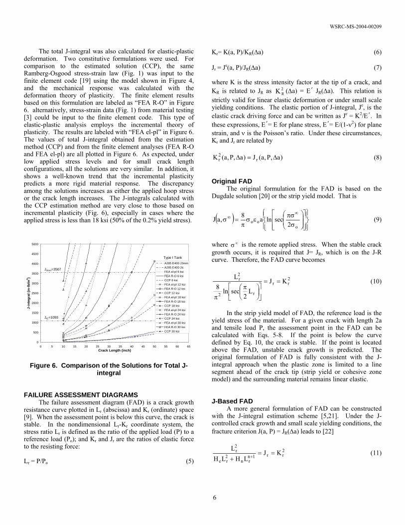
The total J-integral was also calculated for elastic-plastic deformation. Two constitutive formulations were used. For comparison to the estimated solution (CCP), the same Ramberg-Osgood stress-strain law (Fig. 1) was input to the finite element code [19] using the model shown in Figure 4, and the mechanical response was calculated with the deformation theory of plasticity. The finite element results based on this formulation are labeled as “FEA R-O” in Figure 6. alternatively, stress-strain data (Fig. 1) from material testing [3] could be input to the finite element code. This type of elastic-plastic analysis employs the incremental theory of plasticity. The results are labeled with “FEA el-pl” in Figure 6. The values of total J-integral obtained from the estimation method (CCP) and from the finite element analyses (FEA R-O and FEA el-pl) are all plotted in Figure 6. As expected, under low applied stress levels and for small crack length configurations, all the solutions are very similar. In addition, it shows a well-known trend that the incremental plasticity predicts a more rigid material response. The discrepancy among the solutions increases as either the applied hoop stress or the crack length increases. The J-integrals calculated with the CCP estimation method are very close to those based on incremental plasticity (Fig. 6), especially in cases where the applied stress is less than 18 ksi (50% of the 0.2% yield stress).

0

500

1000

1500

2000

2500

3000

3500

4000

4500

5000

0 5 10 15 20 25 30 35 40 45 50 55 60 65Crack Length (inch)

J-in

tegr

al (i

n-lb

/in2 )

A285 E400 J3mmA285 E400 JicFEA el-pl 6 ksiFEA R-O 6 ksiCCP 6 ksiFEA el-pl 12 ksiFEA R-O 12 ksiCCP 12 ksiFEA el-pl 18 ksiFEA R-O 18 ksiCCP 18 ksiFEA el-pl 24 ksiFEA R-O 24 ksiCCP 24 ksiFEA el-pl 30 ksiFEA R-O 30 ksiCCP 30 ksi

JIC=1093

J3mm=3567

Type I Tank

Figure 6. Comparison of the Solutions for Total J-integral

FAILURE ASSESSMENT DIAGRAMS

The failure assessment diagram (FAD) is a crack growth resistance curve plotted in Lr (abscissa) and Kr (ordinate) space [9]. When the assessment point is below this curve, the crack is stable. In the nondimensional Lr-Kr coordinate system, the stress ratio Lr is defined as the ratio of the applied load (P) to a reference load (Po); and Kr and Jr are the ratios of elastic force to the resisting force: Lr = P/Po (5)

Kr= K(a, P)/KR(∆a) (6) Jr = Je(a, P)/JR(∆a) (7) where K is the stress intensity factor at the tip of a crack, and KR is related to JR as (∆a) = E´ J2

RK R(∆a). This relation is strictly valid for linear elastic deformation or under small scale yielding conditions. The elastic portion of J-integral, Je, is the elastic crack driving force and can be written as Je = K2/E´. In these expressions, E´= E for plane stress, E´= E/(1-ν2) for plane strain, and ν is the Poisson’s ratio. Under these circumstances, Kr and Jr are related by

)a,P,a(J)a,P,a(K r2r ∆=∆ (8)

Original FAD

The original formulation for the FAD is based on the Dugdale solution [20] or the strip yield model. That is

( )⎪⎭

⎪⎬⎫

⎪⎩

⎪⎨⎧

⎥⎥⎦

⎤

⎢⎢⎣

⎡⎟⎟⎠

⎞⎜⎜⎝

⎛

σπσ

εσπ

=σ∞

∞

ooo 2

seclna8,aJ (9)

where is the remote applied stress. When the stable crack growth occurs, it is required that J= J

∞σR, which is on the J-R

curve. Therefore, the FAD curve becomes

2rr

r2

2r KJ

L2

secln8L

==

⎥⎦

⎤⎢⎣

⎡⎟⎠⎞

⎜⎝⎛ π

π

(10)

In the strip yield model of FAD, the reference load is the

yield stress of the material. For a given crack with length 2a and tensile load P, the assessment point in the FAD can be calculated with Eqs. 5-8. If the point is below the curve defined by Eq. 10, the crack is stable. If the point is located above the FAD, unstable crack growth is predicted. The original formulation of FAD is fully consistent with the J-integral approach when the plastic zone is limited to a line segment ahead of the crack tip (strip yield or cohesive zone model) and the surrounding material remains linear elastic. J-Based FAD

A more general formulation of FAD can be constructed with the J-integral estimation scheme [5,21]. Under the J-controlled crack growth and small scale yielding conditions, the fracture criterion J(a, P) = JR(∆a) leads to [22]

2rr1n

rn2re

2r KJ

LHLHL

==+ +

(11)

6

WSRC-MS-2004-00209

where and . The function

has been defined in Eq. 3. In this case, the reference load used to define L

( ) ( )aJ/aJH ee = ( ) (aJ/n,aJHn = )J

r should be consistent with that used in the J estimation scheme, and it may depend on the crack length.

This example shows that, in general, the J-based FAD is a function of crack size. It is no longer a single curve as defined by Eq. (10). More specifically, the FAD based on the J estimation scheme depends on the crack length (2a), material hardening exponent (n), type of loading (Eq. 3), and the type of deformation (plane stress or plane strain). As the flaw propagates, a new FAD should be constructed, unless it is judged that the crack increment is small enough not to cause a significant change in the shape of the FAD. Therefore, a family of failure assessment diagrams must be constructed with respect to each crack length. However, the family of failure assessment curves may be shown to collapse to a single curve by selecting a particular reference load [1]. This will be demonstrated in later.

It appears that the FAD approach based on the elastic-plastic J-integral (e.g., Eq. 11) may become more complex and cumbersome when the material-specific curves are to be used [22]. Similar information on flaw stability can be obtained in straightforward approaches such as the J-integral-tearing modulus (J-T) methodology described previously in this paper. API Recommended FAD Approaches

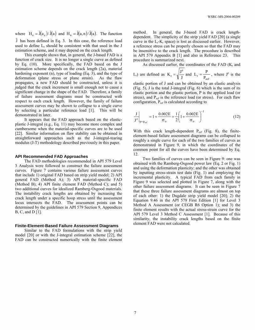
The FAD methodologies recommended in API 579 Level 3 Analysis were followed to construct the failure assessment curves. Figure 7 contains various failure assessment curves that include 1) original FAD based on strip yield model; 2) API general FAD (Method A); 3) API material-specific FAD (Method B); 4) API finite element FAD (Method C); and 5) two additional curves for idealized Ramberg-Osgood materials. The instability crack lengths are obtained by increasing the crack length under a specific hoop stress until the assessment locus intersects the FAD. The assessment points can be determined by the guidelines in API 579 Section 9, Appendices B, C, and D [1]. Finite-Element-Based Failure Assessment Diagrams

Similar to the FAD formulations with the strip yield model [20] or with the J-integral estimation scheme [22], the FAD can be constructed numerically with the finite element

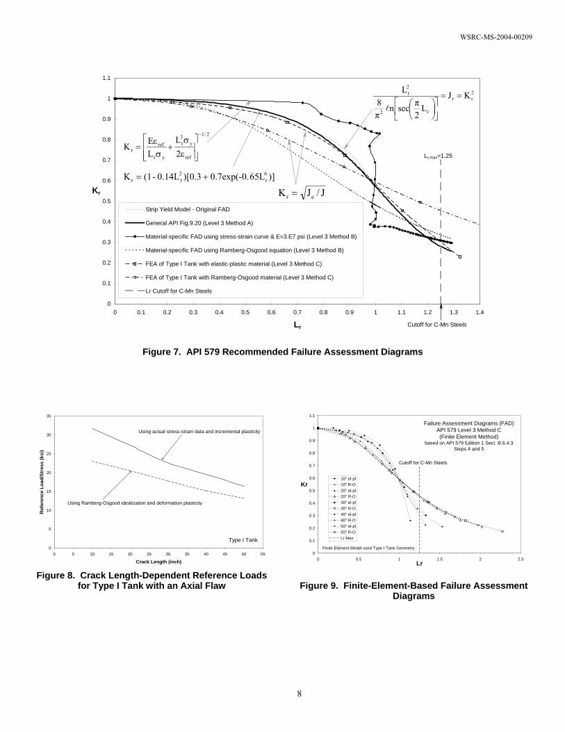
method. In general, the J-based FAD is crack length-dependent. The simplicity of the strip yield FAD [20] (a single curve in the Lr-Kr space) is lost as discussed earlier. However, a reference stress can be properly chosen so that the FAD may be insensitive to the crack length. The procedure is described in API 579 Appendix B [1] and also in Reference 23. This procedure is summarized next.

As discussed earlier, the coordinates of the FAD (Kr and

Lr) are defined as JJK

e

r = and ref

r PPL = , where Je is the

elastic portion of J and can be obtained by an elastic analysis (Fig. 5), J is the total J-integral (Fig. 6) which is the sum of its elastic portion and the plastic portion, P is the applied load (or stress), and Pref is the reference load (or stress). For each flaw configuration, Pref is calculated according to

1

ooppe

E002.0121E002.01

JJ

ref

−

=⎟⎟⎠

⎞⎜⎜⎝

⎛σ

++σ

+= (12)

With this crack length-dependent Pref (Fig. 8), the finite-element-based failure assessment diagrams can be collapsed to roughly a single curve for each of the two families of curves as demonstrated in Figure 9, in which the coordinates of the common point for all the curves have been determined by Eq. 12.

Two families of curves can be seen in Figure 9: one was obtained with the Ramberg-Osgood power law (Eq. 2 or Fig. 1) and using the deformation plasticity; and the other was obtained by inputting stress-strain test data (Fig. 1) and employing the incremental plasticity. A typical FAD from each family in Figure 9 was selected and plotted in Figure 7, along with the other failure assessment diagrams. It can be seen in Figure 7 that these three failure assessment diagrams are almost on top of each other: 1) the Dugdale strip yield model [20]; 2) the Equation 9.46 in the API 579 First Edition [1] for Level 3 Method A Assessment (or CEGB R6 Option 1); and 3) the finite element results with the actual stress-strain curve for the API 579 Level 3 Method C Assessment [1]. Because of this similarity, the instability crack lengths based on the finite element FAD were not calculated.

7

WSRC-MS-2004-00209

0

0.1

0.2

0.3

0.4

0.5

0.6

0.7

0.8

0.9

1

1.1

0 0.1 0.2 0.3 0.4 0.5 0.6 0.7 0.8 0.9 1 1.1 1.2 1.3 1.4

Lr

Kr

Strip Yield Model - Original FAD

General API Fig.9.20 (Level 3 Method A)

Material-specific FAD using stress-strain curve & E=3.E7 psi (Level 3 Method B)

Material-specific FAD using Ramberg-Osgood equation (Level 3 Method B)

FEA of Type I Tank with elastic-plastic material (Level 3 Method C)

FEA of Type I Tank with Ramberg-Osgood material (Level 3 Method C)

Lr Cutoff for C-Mn Steels

Cutoff for C-Mn Steels

Lr,max=1.25

2rr

r2

2r KJ

L2πsecn

π8

L==

⎥⎦

⎤⎢⎣

⎡⎟⎠⎞

⎜⎝⎛

l

)]65L0.7exp(-0. )[0.30.14L-(1K 6r

2rr +=

2/1

ref

y3r

yr

refr 2

LLEK

−

⎥⎥⎦

⎤

⎢⎢⎣

⎡

ε

σ+

σε

=

J/JK er =

Figure 7. API 579 Recommended Failure Assessment Diagrams

0

5

10

15

20

25

30

35

0 5 10 15 20 25 30 35 40 45 50 55

Crack Length (inch)

Ref

eren

ce L

oad/

Stre

ss (k

si)

Using actual stress-strain data and incremental plasticity

Using Ramberg-Osgood idealization and deformation plasticity

Type I Tank

Figure 8. Crack Length-Dependent Reference Loads

for Type I Tank with an Axial Flaw

0

0.1

0.2

0.3

0.4

0.5

0.6

0.7

0.8

0.9

1

1.1

0 0.5 1 1.5 2 2.5Lr

Kr10" el-pl10" R-O20" el-pl20" R-O30" el-pl30" R-O40" el-pl40" R-O50" el-pl50" R-OLr Max


Failure Assessment Diagrams (FAD)API 579 Level 3 Method C(Finite Element Method)

based on API 579 Edition 1 Sect. B.6.4.3Steps 4 and 5

Finite Element Model used Type I Tank Geometry

Figure 9. Finite-Element-Based Failure Assessment

Diagrams

8

WSRC-MS-2004-00209

Determination of Instability Crack Length Based on Failure Assessment Diagram

Figure 10 is used to illustrate the process of obtaining an instability crack length for a given load (or hoop stress in this paper). Two load cases are used for demonstration: 41 MPa (6 ksi) and 124 MPa (18 ksi). The crack length is increased incrementally until the assessment locus intersects the FAD. The calculation procedure for the (Lr, Kr) coordinates of the assessment point can be found in API 579 [1]. The crack length corresponding to the intersection point is the instability crack length under that applied load (or stress). Figure 10 shows the JIC-based instability crack lengths (1.69 and 0.51 meters or 66.4 and 20.2 inches, respectively) determined by the general FAD (API 579 Level 3 Method A Assessment) [1]. Similarly, if a material-specific FAD is used (also see Figure 10), the instability crack length is then obtained by API 579 Level 3 Method B Assessment [1]. It is clear that at these two loading levels, the instability crack lengths determined with the material-specific FAD using the actual tensile test data in Figure 1 are longer than those obtained by the general FAD. However, if the Ramberg-Osgood curve-fit equation is used (α=3.2 and n=5), the resulting instability crack lengths appear to be too conservative (for the two stress levels considered in Figure 10). This may be caused by the Ramberg-Osgood power law performs better in the high stress region but is incapable of following the linear response below the yield stress (see Fig. 1). This observation is also evident in Figure 10, from which it can be seen that the two material-specific curves (based on the actual tensile test data and on the Ramberg-Osgood approximation) agree well when Lr is less than 0.2 or greater than 1.1.

0.0

0.1

0.2

0.3

0.4

0.5

0.6

0.7

0.8

0.9

1.0

1.1

1.2

1.3

0.0 0.1 0.2 0.3 0.4 0.5 0.6 0.7 0.8 0.9 1.0 1.1 1.2 1.3 1.4

Lr

Kr


Lr,max=1.25Instability Crack Length: 66.4 in.

(per API 579 Fig. 9.20)

Instability Crack Length: 20.2 in.(per API 579 Fig. 9.20)

Tensile Test DataMaterial-specific FAD

General API Fig.9.20(Level 3 Method A)

Ramberg-Osgood Material-specific FAD

Locus for σappl = 6 ksi and Jcrit=JIc

Locus for σappl = 18 ksi and Jcrit=JIc

Figure 10. Determination of Instability Crack Length

using FAD Approach

Another FAD approach for determining the instability crack length is suggested by API 579 Level 3 Method D Assessment [1]. It is appropriate for materials which exhibit ductile tearing and the experimental J-R curves are available. The assessment locus uses the J values on the J-R curve

(depending on the amount of crack extension) that produces a fishhook shape as seen in the inset of Figure 11. However, if the J-R curve is cut off for practical reasons, as the J3mm in the present J-T analysis, this type of FAD analysis is identical to the standard procedure with criter J/JK = , in which Jcrit is a constant and is set to the value of J3mm. This is demonstrated in Figure 11. The end points of the “fishhooks” lie on the assessment locus defined by Jcrit = J3mm and the instability crack length is where the end point (tangent) lies on the FAD. This is equivalent to the result for the intersection of the assessment locus and the FAD (see Figure 10).

00.10.20.30.40.50.60.70.80.9

11.11.21.31.41.51.61.71.81.9

22.12.22.3

0 0.1 0.2 0.3 0.4 0.5 0.6 0.7 0.8 0.9 1 1.1 1.2 1.3 1.4

Lr

Kr


Lr,max=1.25

Initial Crack Length = 10 in.

20 in.

29.4 in.

35 in.

Locus for applied stress = 18 ksi and Jcrit = Jcutoff = 3567 in-lb/in2

Instability Crack Length = 29.4 in.

API 579 Fig. 9.20 FAD

FAD Assessment Points based on J-R Curve

0.50.60.70.80.9

11.11.21.31.41.51.61.71.81.9

0.93 0.931 0.932 0.933 0.934 0.935Lr

Kr

Initial Crack Length = 29.4 in.

API 579 Fig. 9.20 FAD

Figure 11. FAD Approach Utilizing J-R Curve Data

COMPARISON OF INSTABILITY CRACK LENGTHS

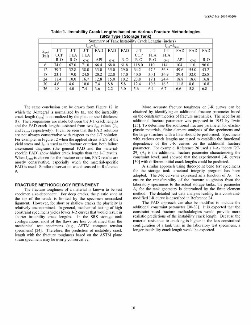
The instability crack lengths determined from all the fracture methodologies including J-T and FAD are listed in Table 1. Figure 6 was used to obtain the finite-element-based instability crack lengths. Extrapolation was used to determine certain instability crack lengths because the finite element mesh (Fig. 4) was designed for cracks from 0.25 to 1.27 meters long (10 to 50 inches).

The finite element method provides the most accurate J-integral results. However, the instability crack lengths based on CCP solution or other estimation schemes are typically used because it is an industrial practice to use approximate solution for the J-integral. Typical J-integral estimation schemes can be found in Electric Power Research Institute (EPRI) publications [e.g., 21], with which the CCP solution [5] shares the same technical basis.

When the applied stress is low, Table 1 shows that the crack instability lengths based on J-T are greater than those determined by FAD, as expected, since the FAD approach generally provides a conservative assessment of flaw stability. However, when the loading is near the yield stress of the material, the results of FAD may overestimate the instability crack length predicted by the J-T method.

9

WSRC-MS-2004-00209

Table 1. Instability Crack Lengths based on Various Fracture Methodologies (SRS Type I Storage Tank)

Summary of Tank Instability Crack Lengths (inches) Jcrit=JIC Jcrit=J3mm

σappl (ksi)

J-T CCP R-O

J-T FEA R-O

J-T FEA σ-ε

FAD

API

FAD

σ-ε

FAD

R-O

J-T CCP R-O

J-T FEA R-O

J-T FEA σ-ε

FAD

API

FAD

σ-ε

FAD

R-O 6 74.0 67.0 71.0 66.4 68.0 61.8 118.0 110. 114. 104. 110. 96.0

12 39.7 32.8 38.0 33.0 35.0 29.0 64.2 47.5 56.8 49.6 55.0 43.2 18 23.1 19.0 24.8 20.2 22.0 17.0 40.0 30.1 36.9 29.4 32.0 25.8 24 11.4 10.0 16.7 12.8 15.0 10.2 23.8 19.1 24.4 18.8 18.6 16.8 30 4.6 4.6 10.0 7.4 8.8 5.8 12.4 10.8 16.3 11.8 8.6 10.8 36 1.8 4.0 7.4 3.6 2.2 3.0 5.6 6.4 6.7 6.6 5.8 6.8

The same conclusion can be drawn from Figure 12, in which the J-integral is normalized by tσo and the instability crack length (acrit) is normalized by the plate or shell thickness (t). The comparisons are made between the J-T crack lengths and the FAD crack lengths assessed from two Jcrit values (JIC and J3mm, respectively). It can be seen that the FAD solutions are not always conservative with respect to the J-T solution. For example, in Figure 12 when the applied stress is 2/3 of the yield stress and JIC is used as the fracture criterion, both failure assessment diagrams (the general FAD and the material-specific FAD) show higher crack lengths than the J-T results. When J3mm is chosen for the fracture criterion, FAD results are mostly conservative, especially when the material-specific FAD is used. Similar observation was discussed in Reference 9. FRACTURE METHODOLOGY REFINEMENT

The fracture toughness of a material is known to be test specimen size-dependent. For deep cracks, the plastic zone at the tip of the crack is limited by the specimen uncracked ligament. However, for short or shallow cracks the plasticity is relatively unconstrained. In general, mechanical testing of high constraint specimens yields lower J-R curves that would result in shorter instability crack lengths. In the SRS storage tank configurations, most of the flaws are less constrained than the mechanical test specimens (e.g., ASTM compact tension specimens) [24]. Therefore, the prediction of instability crack length with the fracture toughness based on the ASTM plane strain specimens may be overly conservative.

More accurate fracture toughness or J-R curves can be obtained by identifying an additional fracture parameter based on the constraint theories of fracture mechanics. The need for an additional fracture parameter was proposed in 1957 by Irwin [25]. To determine the additional fracture parameter for elastic-plastic materials, finite element analyses of the specimens and the large structure with a flaw should be performed. Specimens with various crack lengths are tested to establish the functional dependence of the J-R curves on the additional fracture parameter. For example, Reference 26 used a J-A2 theory [27-29] (A2 is the additional fracture parameter characterizing the constraint level) and showed that the experimental J-R curves [30] with different initial crack lengths could be predicted.

A similar approach using three-point bend test specimens for the storage tank structural integrity program has been adopted. The J-R curve is expressed as a function of A2. To ensure the transferability of the fracture toughness from the laboratory specimens to the actual storage tanks, the parameter A2 for the tank geometry is determined by the finite element method. The detailed test data analysis leading to a constraint-modified J-R curve is described in Reference 24.

The FAD approach can also be modified to include the additional constraint parameter [30-33]. It is expected that the constraint-based fracture methodologies would provide more realistic predictions of the instability crack length. Because the material resistance to cracking is higher in the less constrained configuration of a tank than in the laboratory test specimens, a longer instability crack length would be expected.

10

WSRC-MS-2004-00209

Type I TankApplied Stress = 1/6 σo

0

50

100

150

200

250

300

0.00 0.05 0.10 0.15 0.20 0.25Jcrit/tσo

acrit

/t

J-TJIC

J3mm

• API General FADX Material Specific FAD


0

20

40

60

80

100

120

140

160

0.00 0.05 0.10 0.15 0.20 0.25Jcrit/tσo

acrit

/t

J-T

JIC

J3mm



0102030405060708090

100

0.00 0.05 0.10 0.15 0.20 0.25Jcrit/tσo

acrit

/t

J-TJIC

J3mm



0

10

20

30

40

50

60

0.00 0.05 0.10 0.15 0.20 0.25Jcrit/tσo

acrit

/t

J-T

JIC

J3mm



0

5

10

15

20

25

30

35

0.00 0.05 0.10 0.15 0.20 0.25Jcrit/tσo

acrit

/t

J-TJIC

J3mm


Type I TankApplied Stress ≈ σo

0

2

4

6

8

10

12

14

16

18

0.00 0.05 0.10 0.15 0.20 0.25Jcrit/tσo

acrit

/t

J-TJIC

J3mm


Figure 12. Comparison of Predicted Instability Crack Lengths from J-T and FAD for Given Jcrit in Type I Tanks DISCUSSION AND CONCLUDING REMARKS • The finite element method provides the most accurate J-

integral solution for the structural components containing flaws under service loads.

• Comparing the J-integral solution from the finite element analysis with the actual tensile property input, the CCP approximation with a curvature correction was shown to be accurate for crack length less than 7.62 meters (30 in.) and under hoop stress loading up to about ½ of the yield stress (124 MPa or 18 ksi) of the material (A285 carbon steel).

• The predicted instability crack lengths depend on the specific FAD methods.

• The FAD constructed from the finite element results (API

579 Method C Assessment) is consistent with the original FAD based on the strip yield model and the general FAD formulation in the API 579 Method A Assessment (or CEGB R6 Option 1).

• The ductile tearing FAD (API 579 Method D Assessment) is equivalent to a standard FAD approach with a constant Jcrit.

• Instability crack lengths based on the FAD analysis are not always conservative with respect to the J-T analysis using estimation methods such as the CCP approximation.

• Applying a factor of safety to the actual loads with the FAD approach might lead to a non-conservative estimate (with respect to the J-integral estimation methods) of the instability flaw size. This is implied by the results in

11

WSRC-MS-2004-00209

Figure 12. • The FAD-based instability crack lengths are bounded by

the results of the J-T method (specified in the API 579 Method E Assessments) with accurate finite element J-integral solutions.

• The J-T method with an accurate finite element J-integral solution will maximize the stable crack length predicted for the storage tanks. As a result, the tank fill limit may be increased.

• The instability crack lengths would be longer and the safety margin would be increased if the constraint-modified J-R curve is used, especially for large structures such as the SRS storage tanks.

ACKNOWLEDGMENTS This research was supported by the Savannah River

Technology Center and the Savannah River Site High Level Waste Division. The work was funded by the United States Department of Energy under Contract Number DE-AC09-96SR18500. Additional support from DOE Office of Science Environmental Management Science Program (EMSP) is acknowledged.

REFERENCES [1] “Fitness-for-Service API Recommended Practice 579

First Edition,” American Petroleum Institute, API Publishing Services, Washington, D. C., January 2000.

[2] Milne, I, Ainsworth, R. A., Dowling, A. R., and Stewart, A. T., “Assessment of the Integrity of Structures Containing Defects,” Central Electricity Generating Board Report R/H/R6-Rev. 3, May 1986; Also in International Journal of Pressure Vessel & Piping, Vol. 32, pp. 3-104, 1988.

[3] Subramanian, K. H. and Duncan, A. J., “Tensile Properties for Application to Type I and Type II Waste Tank Flaw Stability Analysis (U),” WSRC-TR-2000-00232, Westinghouse Savannah River Company, Aiken, SC, July 2000.

[4] Subramanian, K. H. Duncan, A. J. and Sindelar, R. L., “Mechanical Properties for Application to Type I and Type II Waste Tank Flaw Stability Analysis (U),” WSRC-TR-99-00416 Rev. 1, Westinghouse Savannah River Company, Aiken, SC, October 2000.

[5] Shih, C.F. and Hutchinson, J.W., "Fully Plastic Solutions and Large Scale Yielding Estimates for Plane Stress Crack Problems," Trans. American Society of Mechanical Engineers, Journal of Engineering Materials and Technology, Series H, Vol. 98, pp. 289-295, 1976.

[6] Lam, P. S. and Sindelar, R. L., “J-Integral Based Flaw Stability Analysis of Mild Steel Storage Tanks,” in Fracture, Fatigue and Weld Residual Stress, J. Pan, Ed., American Society of Mechanical Engineers, PVP-Vol. 393, pp. 139-143, 1999.

[7] Lam, P. S. and Sindelar R. L., “Flaw Stability in Mild Steel Tanks in the Upper-Shelf Ductile Range – Part II: J-Integral Based Fracture Analysis,” ASME Journal of

Pressure Vessel Technology, Vol. 122, pp. 169-173, May 2000.

[8] Mehta, H.S., "Fracture Mechanics Evaluation of Potential Flaw Indications in the Savannah River L, P and K Tanks," SASR#86-64 (DRF137-0010), General Electric Nuclear Energy, San Jose, CA, October 1989.

[9] Anderson, T. L., Fracture Mechanics: Fundamentals and Applications, 2nd Edition, CRC Press, Boca Raton, Florida, 1995.

[10] Kanninen, M. F. and Popelar, C. H., Advanced Fracture mechanics, Oxford University Press, New York, New York, 1985.

[11] Lam, P. S., Sindelar, R. L., and Awadalla, N.G., "Acceptance Criteria for In-service Inspection of Heat Exchanger Head and Shell Components,” in Fatigue and Fracture of Aerospace Structural Materials, A. Nagar and A.-Y. Kuo, Eds., American Society of Mechanical Engineers, AD-Vol. 36, pp. 43-57, 1993.

[12] Erdogan, F., "Theoretical and Experimental Study of Fracture in Pipelines Containing Circumferential Flaws," DOT-RSPA-DMA-50/83/3, Department of Mechanical Engineering and Mechanics, Lehigh University, Bethlehem, PA, prepared for US Department of Transportation, August 1982.

[13] Rooke, D. P., and Cartwright, D. J., Compendium of Stress Intensity Factors, Her Majesty’s Stationery Office, London, 1976.

[14] Tada, H., Paris, P.C. and Irwin, G.R., The Stress Analysis of Cracks Handbook, Second Edition, Pages 33.3, 33.4, 33.6 and 34.1, Paris Productions Incorporated (and Del Research Corporation), Saint Louis, MO, 1985.

[15] Green, D. and Knowles, J., "The Treatment of Residual Stress in Fracture Assessment of Pressure Vessels," Journal of Pressure Vessels Technology, Vol. 116, pp. 345-352, 1994.

[16] Dong, P., Zhang, J., Hong, J. K., and Brust, F. W., “Task 1: Residual Stresses and Stress Intensity Factors for Single Butt Welds,” Final Report No. G003824-01, Battelle Memorial Institute, Columbus, OH 43201, September 1999.

[17] Dong, P., Zhang, J., Hong, J. K., and Brust, F. W., “Task 2: Residual Stresses and Stress Intensity Factors for Intersecting Horizontal and Vertical Welds,” Final Report No. G003824-02, Battelle Memorial Institute, Columbus, OH 43201, November 1999.

[18] Dong, P., Zhang, J., Hong, J. K., and Brust, F. W., “Task 3: Residual Stresses and Stress Intensity Factors for Weld Repairs and Attachments,” Final Report No. G003824-03, Battelle Memorial Institute, Columbus, OH 43201, February 29, 2000.

[19] ABAQUS/Standard, Version 5.8, Hibbitt, Karlsson & Sorensen, Inc., Pawtucket, Rhode Island, 1998.

[20] Dugdale, D. S., “Yielding of Steels Containing Slits,” Journal of Mechanics and Physics of Solids, Vol. 8, pp. 100-108, 1960.

[21] Kumar, V., German, M. D., and Shih, C. F., “An Engineering Approach for Elastic-Plastic Fracture

12

WSRC-MS-2004-00209

Analysis,” EPRI Topical report NP-1931, Electric Power Research Institute, Palo Alto, California, July 1981

[22] Shih, C. F., Kumar, V., and German, M. D., “Studies on the Failure Assessment Diagram Using the Estimation Method and J-Controlled Crack Growth Approach,” in Elastic-Plastic Fracture, Second Symposium, Vol. II, ASTM STP 803, C. F. Shih and J. P. Gudas, Eds., American Society for Testing and Materials, pp. II-239-II-261, 1983.

[23] Scott, P. M., Anderson, T. L., Osage, D. A., and Wilkowski, G. M., “Review of Existing Fitness-for-Service Criteria for Crack-Like Flaws,” WRC Bulletin 430, Welding Research Council, Inc., New York, April 1988.

[24] Lam, P. S, Chao, Y. J., Zhu, X.-K., Kim, Y., Sindelar, R. L., “Determination of Constraint-modified J-R Curves for Carbon Steel Storage Tanks,” ASME Journal of Pressure Vessel Technology, pp. 136-143, 2003.

[25] Irwin, G. R., “Analysis of Stress and Strain Near the End of a Crack Traversing a Plate,” Journal of Applied mechanics, Vol. 24, pp. 361-364, 1957.

[26] Chao, Y. J., Zhu, X. K., Lam, P.-S., Louthan, M. R., and Iyer, N. C., “Application of the Two-Parameter J-A2 Description to Ductile Crack Growth,” in Fatigue and Fracture Mechanics: 31st Volume, ASTM STP 1389, G. R. Halford and J. P. Gallagher, Eds., American Society for Testing and Materials, West Conshohocken, PA, pp. 165-182, 2000.

[27] Yang, S., Chao, Y. J. and Sutton, M. A., “Higher order asymptotic crack tip fields in a power-law hardening

material,” Engineering Fracture Mechanics, Vol. 45, pp. 1-20, 1993.

[28] Yang, S., Chao, Y. J. and Sutton, M. A., “Complete Theoretical Analysis for Higher Order Asymptotic Terms and the HRR Zone at a Crack Tip for Mode I and Mode II Loading of a Hardening Material,” Acta Mechanica, Vol. 98, pp. 79-98, 1993.

[29] Chao, Y. J., Yang, S. and Sutton, M. A., “On The Fracture of Solids Characterized by One or Two Parameters: Theory and Practice,” Journal of the Mechanics and Physics of Solids, Vol. 42, pp. 629-647, 1994.

[30] Joyce, J. A. and Link, R. E., “Application of two parameter elastic-plastic fracture mechanics to analysis of structures,” Engineering Fracture Mechanics, Vol. 57, pp. 431-446, 1997.

[31] MacLennan, I. J. and Hancock, J. W., “Constraint-based Failure Assessment Diagrams,” Proceedings Royal Society of London, Series A, Vol. 451, pp. 757-777, 1995.

[32] Hancock, J. W. and Kekal, A., “The Application of Constraint Based Fracture Mechanics to Engineering Structures,” Nuclear Engineering and Design, Vol. 184, pp. 77-88, 1998.

[33] Ainsworth, R. A. and O’Dowd, N. P., “A Framework for Including Constraint Effects in the Failure Assessment Diagram Approach for Fracture Assessment,” in Fracture Mechanics Applications, H. S. Mehta, Ed., American Society of Mechanical Engineers, PVP-Vol. 287/MD-Vol. 47, pp. 137-145, 1994.

13

Documents

Comparison of Fracture Methodologies for Flaw Stability Analysis of Storage Tanks