Embed Size (px)
Citation preview
LEOPOLD FRANZENS UNIVERSITY OF INNSBRUCK
MASTER THESIS
Comparison of Embedding Strategies forthe Quantum Approximate Optimization
Algorithm
Author:Michael FELLNER, BSc
Supervisor:Priv.-Doz. Dr. Wolfgang
LECHNER
A thesis submitted in fulfillment of the requirementsfor the degree of Master of Science
in the
Quantum Optimization GroupInstitute for Theoretical Physics
August 11, 2020


iii
Declaration of AuthorshipI, Michael FELLNER, declare that this thesis titled “Comparison of Embedding Strate-gies for the Quantum Approximate Optimization Algorithm” and the work pre-sented in it are my own. I confirm that:
• This work was done wholly or mainly while in candidature for a research de-gree at this university.
• Where any part of this thesis has previously been submitted for a degree orany other qualification at this university or any other institution, this has beenclearly stated.
• Where I have consulted the published work of others, this is always clearlyattributed.
• Where I have quoted from the work of others, the source is always given. Withthe exception of such quotations, this thesis is entirely my own work.
• I have acknowledged all main sources of help.
• Where the thesis is based on work done by myself jointly with others, I havemade clear exactly what was done by others and what I have contributed my-self.
Signed:
Date:

v
LEOPOLD FRANZENS UNIVERSITY OF INNSBRUCK
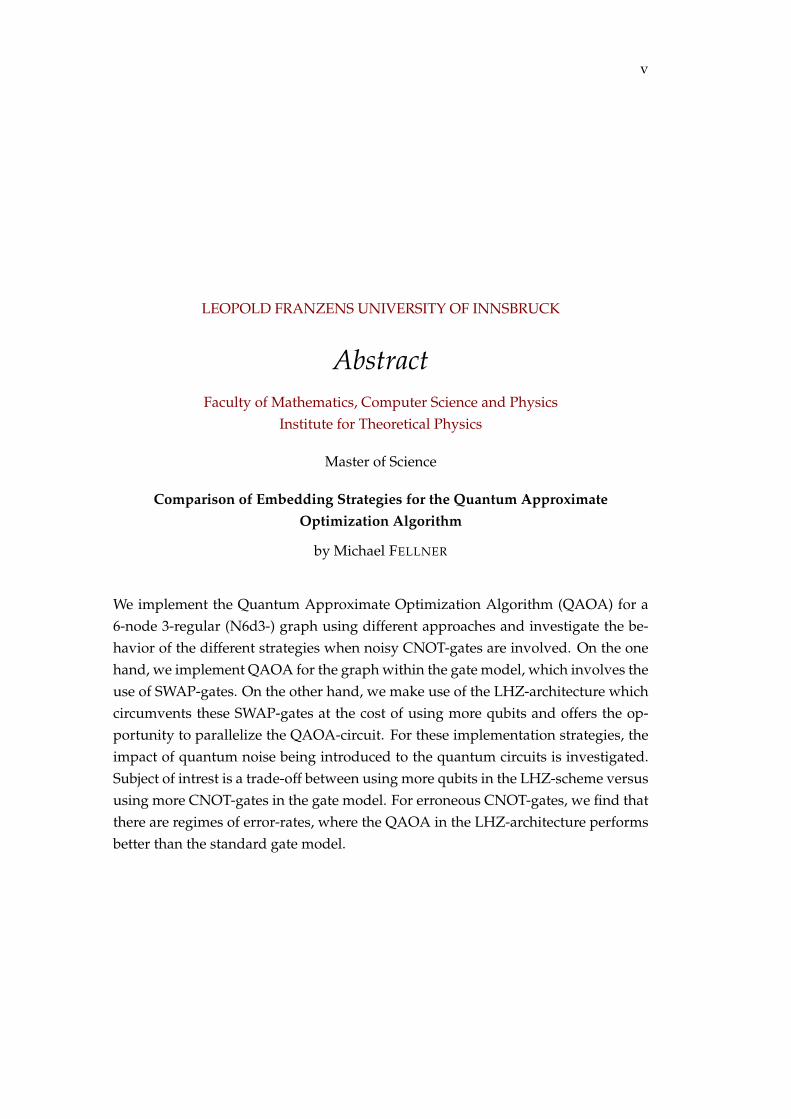
AbstractFaculty of Mathematics, Computer Science and Physics
Institute for Theoretical Physics
Master of Science
Comparison of Embedding Strategies for the Quantum ApproximateOptimization Algorithm
by Michael FELLNER
We implement the Quantum Approximate Optimization Algorithm (QAOA) for a6-node 3-regular (N6d3-) graph using different approaches and investigate the be-havior of the different strategies when noisy CNOT-gates are involved. On the onehand, we implement QAOA for the graph within the gate model, which involves theuse of SWAP-gates. On the other hand, we make use of the LHZ-architecture whichcircumvents these SWAP-gates at the cost of using more qubits and offers the op-portunity to parallelize the QAOA-circuit. For these implementation strategies, theimpact of quantum noise being introduced to the quantum circuits is investigated.Subject of intrest is a trade-off between using more qubits in the LHZ-scheme versususing more CNOT-gates in the gate model. For erroneous CNOT-gates, we find thatthere are regimes of error-rates, where the QAOA in the LHZ-architecture performsbetter than the standard gate model.


vii
AcknowledgementsForemost, I would like to express my appreciation to my research supervisor Wolf-gang Lechner, for arousing my interest in the field of quantum optimization, givingme the opportunity to do my Master thesis in his research group and his continuoussupport throughout the work progress. My thanks also go to all members of theQuantum Optimization Group in Innsbruck for the enjoyable work environment,the excellent collaboration and many fruitful discussions.
Furthermore, great thanks go to my friends and colleagues who supported andencouraged me throughout my studies. I particularly want to mention AndreasKlingler, who accompanied me from the very beginning of our studies until gradu-ation.
I do not want to miss to thank my physics teacher in high school, ChristianPronegg, for making me aware of the beauty of physical concepts, supporting mein his courses and (maybe unconsciously) prompting me to choose physics as myfield of studies.
Finally, I would like to express my profound gratitude to my family, for theirmental and financial support, their encouragement and their never-ending kindnessand love.

ix
Contents
Declaration of Authorship iii
Abstract v
Acknowledgements vii
1 Introduction 11.1 Motivation . . . . . . . . . . . . . . . . . . . . . . . . . . . . . . . . . . . 11.2 Thesis Outline . . . . . . . . . . . . . . . . . . . . . . . . . . . . . . . . . 21.3 Mentions . . . . . . . . . . . . . . . . . . . . . . . . . . . . . . . . . . . . 2
2 Theoretical Background 32.1 Basic Concepts of Quantum Mechanics . . . . . . . . . . . . . . . . . . 3
2.1.1 Quantum States and Density Matrices . . . . . . . . . . . . . . . 32.1.2 Quantum Operators and Gates . . . . . . . . . . . . . . . . . . . 42.1.3 Quantum Fidelity . . . . . . . . . . . . . . . . . . . . . . . . . . . 62.1.4 Quantum Noise . . . . . . . . . . . . . . . . . . . . . . . . . . . . 7
2.2 The Quantum Approximate Optimization Algorithm . . . . . . . . . . 82.2.1 Basics and Definitions . . . . . . . . . . . . . . . . . . . . . . . . 82.2.2 The Algorithm . . . . . . . . . . . . . . . . . . . . . . . . . . . . 102.2.3 Remarks on QAOA . . . . . . . . . . . . . . . . . . . . . . . . . . 10
2.3 The Ising-Model and NP-hard Problems . . . . . . . . . . . . . . . . . . 112.3.1 Complexity of Computational Problems . . . . . . . . . . . . . . 112.3.2 Ising Spin Glasses . . . . . . . . . . . . . . . . . . . . . . . . . . . 122.3.3 Example: Graph Partitioning . . . . . . . . . . . . . . . . . . . . 13
2.4 The LHZ-architecture . . . . . . . . . . . . . . . . . . . . . . . . . . . . . 152.4.1 Translating the Spin-Glass Hamiltonian . . . . . . . . . . . . . . 152.4.2 Constraints on Closed Loops . . . . . . . . . . . . . . . . . . . . 162.4.3 External Magnetic Fields . . . . . . . . . . . . . . . . . . . . . . . 18
3 Embedding Strategies for the QAOA 193.1 The Problem to be implemented . . . . . . . . . . . . . . . . . . . . . . 19
3.1.1 Our Example: A 3-regular Graph . . . . . . . . . . . . . . . . . . 193.1.2 QAOA-Operators for our Problem . . . . . . . . . . . . . . . . . 20
3.2 Implementation of Interactions . . . . . . . . . . . . . . . . . . . . . . . 213.3 The Gate Model . . . . . . . . . . . . . . . . . . . . . . . . . . . . . . . . 23
x
3.4 LHZ-Proposal . . . . . . . . . . . . . . . . . . . . . . . . . . . . . . . . . 253.4.1 Finding Constraints and compiling the LHZ-scheme . . . . . . 253.4.2 Implementation of the Circuit on a Square Lattice . . . . . . . . 273.4.3 Parallelization of the LHZ-ansatz for QAOA . . . . . . . . . . . 27
4 Simulations and Results 314.1 Simulation Methods . . . . . . . . . . . . . . . . . . . . . . . . . . . . . 31
4.1.1 Metropolis Algorithm . . . . . . . . . . . . . . . . . . . . . . . . 314.1.2 Nelder-Mead Algorithm . . . . . . . . . . . . . . . . . . . . . . . 32
4.2 General Framework . . . . . . . . . . . . . . . . . . . . . . . . . . . . . . 344.2.1 The cirq-Package . . . . . . . . . . . . . . . . . . . . . . . . . . . 344.2.2 Noise-model for the Simulations . . . . . . . . . . . . . . . . . . 344.2.3 Simulation Parameters . . . . . . . . . . . . . . . . . . . . . . . . 354.2.4 Initial Fidelity . . . . . . . . . . . . . . . . . . . . . . . . . . . . . 354.2.5 Calculation of Errorbars . . . . . . . . . . . . . . . . . . . . . . . 37
4.3 QAOA with perfect CNOT-gates . . . . . . . . . . . . . . . . . . . . . . 374.4 QAOA with imperfect (noisy) CNOT-gates . . . . . . . . . . . . . . . . 38
4.4.1 Fidelity vs. QAOA depth . . . . . . . . . . . . . . . . . . . . . . 394.4.2 Fidelity vs. Error-rate . . . . . . . . . . . . . . . . . . . . . . . . 404.4.3 Performance of the parallelized LHZ-scheme . . . . . . . . . . . 41
4.5 Discussion and Summary of the Results . . . . . . . . . . . . . . . . . . 42
5 Outlook and conclusion 45
A Graph Instances for the Simulations 47
Bibliography 49
1
Chapter 1
Introduction
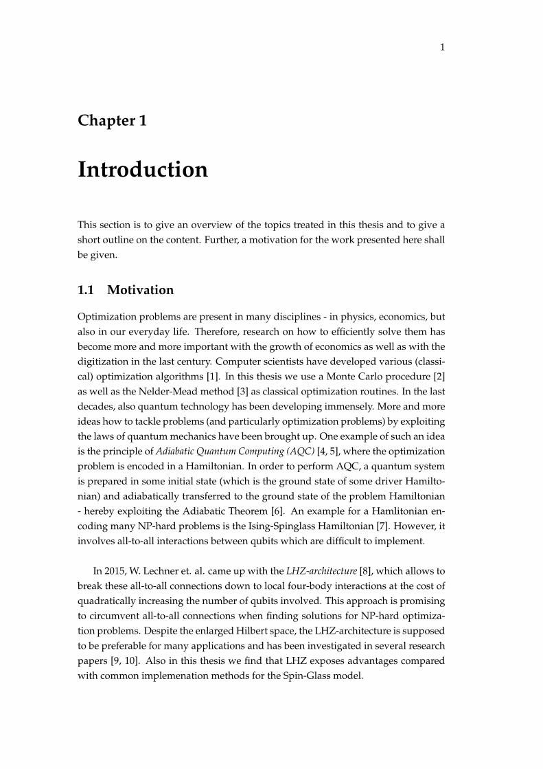
This section is to give an overview of the topics treated in this thesis and to give ashort outline on the content. Further, a motivation for the work presented here shallbe given.
1.1 Motivation
Optimization problems are present in many disciplines - in physics, economics, butalso in our everyday life. Therefore, research on how to efficiently solve them hasbecome more and more important with the growth of economics as well as with thedigitization in the last century. Computer scientists have developed various (classi-cal) optimization algorithms [1]. In this thesis we use a Monte Carlo procedure [2]as well as the Nelder-Mead method [3] as classical optimization routines. In the lastdecades, also quantum technology has been developing immensely. More and moreideas how to tackle problems (and particularly optimization problems) by exploitingthe laws of quantum mechanics have been brought up. One example of such an ideais the principle of Adiabatic Quantum Computing (AQC) [4, 5], where the optimizationproblem is encoded in a Hamiltonian. In order to perform AQC, a quantum systemis prepared in some initial state (which is the ground state of some driver Hamilto-nian) and adiabatically transferred to the ground state of the problem Hamiltonian- hereby exploiting the Adiabatic Theorem [6]. An example for a Hamlitonian en-coding many NP-hard problems is the Ising-Spinglass Hamiltonian [7]. However, itinvolves all-to-all interactions between qubits which are difficult to implement.
In 2015, W. Lechner et. al. came up with the LHZ-architecture [8], which allows tobreak these all-to-all connections down to local four-body interactions at the cost ofquadratically increasing the number of qubits involved. This approach is promisingto circumvent all-to-all connections when finding solutions for NP-hard optimiza-tion problems. Despite the enlarged Hilbert space, the LHZ-architecture is supposedto be preferable for many applications and has been investigated in several researchpapers [9, 10]. Also in this thesis we find that LHZ exposes advantages comparedwith common implemenation methods for the Spin-Glass model.
2 Chapter 1. Introduction
A relatively new approach for tackling combinatorial optimization problems dueto E. Farhi et. al. aims at finding an approximate solution to an optimization problemand is therefore called the Quantum Approximate Optimization Algorithm (QAOA). Itwas presented in 2014 [11] and has become more and more obvious to be a promisingapproach to tackle classically hard optimization problems. It can be understood asa generalization of a trotterized version of AQC [12]. As a hybrid quantum-classicalapproach, it is one of the strategies that are most likely to prove quantum advantageon near-term devices [13].
In this thesis, we implement a 3-regular graph with 6 nodes (N6d3-graph) fordifferent approaches and simulate QAOA on that problem. We seek for its groundstate (by viewing the graph’s nodes as interacting spins). Using QAOA for solvingthis problem, we investigate the performance of QAOA with different implementa-tion strategies for the Spin-Glass model. On the one hand, we directly implement theinteractions given by the edges of the graph (gate model), tackling non-local interac-tions by using SWAP-gates. On the other hand, we use LHZ to circumvent non-localinteractions by introducing three more qubits. We are interested in which approachQAOA performs better when noisy CNOT-gates are used, depending on the extentof the quantum noise on the gates.
1.2 Thesis Outline
The rest of the thesis is organized as follows. In chapter 2, we will review some basicsof quantum mechanics and introduce the QAOA as well as the LHZ-architecture. Inchapter 3, the problem considered in this thesis is introduced. Furthermore, thedifferent approaches to implement QAOA are discussed. We discuss the simulationframework and the results in chapter 4. Finally, we summarize the most importantinsights in chapter 5 and give an outlook on possible future research on the topictreated in this thesis.
1.3 Mentions
The figures in this thesis presenting graphs and simulation results were created withMatplotlib for Python [14]. The schematic figures were created with the TikZ-Package [15]. For the ones involving quantum circuits the Quantikz package forLatex [16] was used in addition. For the simulation of quantum circuits, we used thefreely available Python package cirq [17].
3
Chapter 2
Theoretical Background
In this chapter, we want to give an introduction to the theory of the basic physicalconcepts used in this thesis. That is, first of all, giving an outline of some concepts ofquantum mechanics and quantum information used in this thesis. Moreover, we willexplain the basics of the Quantum Approximate Optimization Algorithm (QAOA)[11], which is the essential ingredient of this thesis. Also, we introduce the notion ofcomplexity classes very briefly. Furthermore, the encoding of NP-hard problems inan Ising model [7] plays an important role, which in turn leads to the introductionof the LHZ-architecture [8]. The LHZ-architecture is the second main idea used inthis work. These concepts will also be introduced in this section.
2.1 Basic Concepts of Quantum Mechanics
Here, we want to sketch some conventions and definitions from quantum informa-tion that play an important role in this thesis. This involves quantum states anddensity matrices as well as quantum operators and -gates. In addition, we introducemethods and notations for the description of quantum noise. An important mea-sure for the quality of approximate solutions is the quantum fidelity. The quantumfidelity can be defined in various ways (cf. [18], [19], [20]). Therefore its definitionused here shall also be clearified in this section. For a more basic introduction toquantum information, the reader is referred to the standard literature such as [21]or [22]. More advanced topics on Quantum Information in particular are covered in[20].
2.1.1 Quantum States and Density Matrices
A quantum state lives in a Hilbert spaceH and describes a physical system quantummechanically. In particular, it provides a probability distribution for the outcome onany possible measurement on the physical system described by the state. For a qubit|ψ〉, which can be written as
|ψ〉 = α |0〉+ β |1〉 (2.1)
with α, β ∈ C and |α|2 + |β|2 = 1, we have dim(H) = 2 and H ∼= C2, and moregenreally for n qubits, dim(H) = 2n and H ∼= C2n, respectively. A quantum state
4 Chapter 2. Theoretical Background
like the qubit |ψ〉 that can be described by a single ket, is called a pure state, andcontains only quantum correlation [20]. However, there exist states that consist ofa classical mixture of pure states, which are called mixed states. Mixed states arerepresented by a density matrix ρ with the following properties:
ρ† = ρ (hermiticity) (2.2a)
ρ ≥ 0 (positivity) (2.2b)
ρ2 = ρ (projector) (2.2c)
Tr(ρ) = 1 (normalization) (2.2d)
In particular, a density matrix can be decomposed in the pure states by
ρ = ∑i
pi |ψi〉 〈ψi| , (2.3)
where pi with 0 ≤ pi ≤ 1 and ∑i pi = 1 can be viewed as probabilities and |ψi〉denote the possible pure states of the system. The density matrix of a pure state isnothing but the projector on the corresponding ket:
ρ = |ψ〉 〈ψ| . (2.4)
Mixed states are used to describe quantum noise such as bit flips, dephasing etc.(cf. sec. 2.1.4) because quantum noise involves a classical mixture of states. Theexpectation value when measuring some observable O on a density matrix ρ is givenby
〈O〉ψ = Tr(ρO) = ∑i
pi 〈ψi|O|ψi〉 . (2.5)
For a pure state, this simplifies to
〈O〉ψ = 〈ψ|O|ψ〉 . (2.6)
2.1.2 Quantum Operators and Gates
A linear quantum operator A is a linear map
A : H −→ H : |ψ〉 7→ A |ψ〉 (2.7)
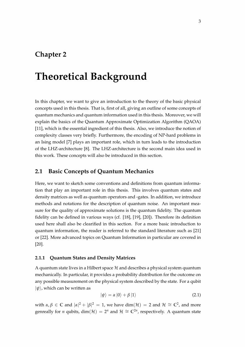
and can (as any linear map) also be written in matrix representation. The set ofeigenvalues of this matrix is called the spectrum σ of the operator. If A is hermitian, i.e. it has real eigenvalues, it is called an observable. If an observable is measured withoutcome λi ∈ σ, the state is projected into the corresponding eigenstate, accordingto the postulates of quantum mechanics [21].Quantum gates correspond to unitary operators that act on one or more qubit(s). Theyrepresent the basic operations which a quantum computer can perform on qubits.
2.1. Basic Concepts of Quantum Mechanics 5
Gate label Matrix representation Circuit symbol
Rx(θ) = e−i2 θσx
(cos θ
2 −i sin θ2
−i sin θ2 cos θ
2
)Rx(θ)
Rz(θ) = e−i2 θσz
(e−i θ
2 00 ei θ
2
)
Rz(θ)
CNOTc,t
1 0 0 00 1 0 00 0 0 10 0 1 0
c
t
SWAPi,j
1 0 0 00 0 1 00 1 0 00 0 0 1
i
j
=i
j
TABLE 2.1: A list of quantum gate operators.
Examples for quantum gates are the Pauli-operators
σx =
(0 11 0
), σy =
(0 −ii 0
)and σz =
(1 00 −1
). (2.8)
They can, due to their hermiticity, also be viewed as observables. The paulimatricesfulfill the relation
σiσj = δij1+ ∑k=x,y,z
εijkσk, (2.9)
where εijk denotes the Levi-Civita-symbol. This relation can be easily proven byplugging the matrices into the relation.
The eigenstates of σz will be denoted by |0〉 and |1〉, while the eigenstates of σx
read |−〉 and |+〉 throughout this thesis. The pauli matrices themselves representquantum gates and are also a ingredient for rotation gates.
We distinguish between single-qubit gates and multiple-gubit gates. They arecharacterized by the number of qubits they act on. In table 2.1, some importantexamples for quantum gates used in this thesis are listed. The Rx and the Rz gatecorrespond to a rotation of a state on the Bloch sphere (cf. [20]) around the x- andz-axis, respectively. The CNOT-gate, acting on two qubits, causes a flip on the target(t) qubit iff the control qubit (c) is set. The SWAP gate, also acting on two qubits,swaps the state of two qubits. Note that SWAPi,j = SWAPj,i.
6 Chapter 2. Theoretical Background
2.1.3 Quantum Fidelity
When approximating a quantum state (which we are going to do within this thesis),we need some measure to quantify the quality of an approximation. Therefore, wehave to introduce a measure of distance between two quantum states in the Hilbertspace H. Here, we use the quantum fidelity as a distance measure. Consider two(generally mixed) states represented by the density matrices ρ and σ. Then the fi-delity F of these states is defined to be
F(σ, ρ) := Tr√√
ρσ√
ρ, (2.10)
where we stick to the convention used in [20]. Here, the square root of a positivesemidefinite and hermitian (these properties are fulfilled for density matrices) ma-trix A is defined such that
A =√
A√
A. (2.11)
Let further U be the unitary matrix that diagonalizes A, i. e. A = UDU† where D isa diagonal matrix. Then, the square root of A is given by
√A = U
√DU†, (2.12)
where√
D is obtained by taking the square root elementwise. Due to normalization,the fidelity is bounded, i. e.
0 ≤ F ≤ 1. (2.13)
If one of the states is considered to be pure, i. e. σ = |ψ〉 〈ψ| for some state |ψ〉,expression (2.10) simplifies to
F(|ψ〉 , ρ) = Tr
√√|ψ〉 〈ψ|ρ
√|ψ〉 〈ψ| =
√〈ψ|ρ|ψ〉Tr
√|ψ〉 〈ψ| =
=√〈ψ|ρ|ψ〉.
(2.14)
If also the second state is a pure state, i. e. ρ = |φ〉 〈φ|, we further simplify andobtain
F(|ψ〉 , |ϕ〉) =√〈ϕ|ψ〉 〈ψ|ϕ〉 = |〈ϕ|ψ〉 |, (2.15)
which is the absolute value of the overlap between the two states. The above defini-tions measure the distance of a state to a single other state. For our purposes, we alsowant to see how close a state is to a span of other states, i. e. a more dimensionalsubspace. This is necessary, if we want to measure how far some state is from a de-generate ground state of a Hamiltonian. Let Φ = |φi〉n
i=1 with n < N be a set ofstates that span a subspace of the H and SΦ = span(Φ). For simplicity, we assumethem to be orthonormal, such that for n = N, the states in Φ form an orthonormal
2.1. Basic Concepts of Quantum Mechanics 7
basis of the HilbertspaceH. We define
F(SΦ, ρ) :=
√n
∑i=1〈φi|ρ|φi〉 (2.16)
as the overlap of the span with a general state ρ. It is easy to see that also thisexpression is bounded from above by 1:
F2(SΦ, ρ) =n
∑i=1〈φi|ρ|φi〉 ≤
N
∑i=1〈φi|ρ|φi〉 =
N
∑i,j=1
pj 〈φi|φj〉 〈φj|φi〉 =
=N
∑i,j=1
pjδij =N
∑i=1
pi = 1.
Here, δij denotes the Kronecker-Delta. We have made use of the the fact that Φ is aset of orthonormal vectors (i. e. 〈φi|φj〉 = δij). As ρ is positive semidefinite, it is alsoclear that F ≥ 0. For a pure state ρ = |ψ〉 〈ψ|, eq. (2.16) simplifies to
F(SΦ, |ψ〉) =√
n
∑i=1|〈φi|ψ〉 |2. (2.17)
These generalized definitions of the quantum fidelity allow us, for example, tocheck how close a state is to a degenerate ground state. This will be necessary forthe Ising-model, whose ground state is twice degenerate. As a last point, note thatthe square of the fidelity represents the probability to find the system in the desiredstate. For example, if we compare a state |ψ〉 with the ground state |φ0〉 of someHamiltonian, the quantity F2(|ψ〉 , |φ0〉) corresponds to the probability to obtain theground state when measuring the energy of the system. This, of course, is also truefor the more general case involving density matrices.
2.1.4 Quantum Noise
If one does not deal with closed quantum systems but let them interact with theenvironment (which always happens in experimental realizations), the systems maysuffer from unwanted interactions with the environment. These unwanted processesappear under the name of quantum noise. In order to describe the (in)coherent evo-lution of quantum states, we introduce the concept of quantum channels. A quantumchannel E is a completely positive and trace-preserving map (CPTP-map) that mapsdensity matrices to density matrices
ρ 7→ E(ρ) (2.18)
for some density matrix ρ. A quantum channel can be seen as a description of themost general form of a quantum system. Due to Choi’s theorem on CPTP-maps [23],
8 Chapter 2. Theoretical Background
the quantum channel E must take the form
E(ρ) =m
∑k=1
AkρA†k , (2.19)
where the operators Ki are called Kraus operators and fulfill the relation
m
∑k=1
A†k Ak = 1. (2.20)
Condition (2.20) ensures that E is trace preserving, i. e. that E maps a density matrixto another valid density matrix. The integer number m is called the Kraus-rank of thechannel E .
One example for a quantum channel is the quantum channel Elp describing a bit-flip with probability p on a qubit described by the density matrix ρ. It is definedby
Elp (ρ) = p · σxρσx + (1− p) · ρ. (2.21)
This channel can be expressed in the form (2.19) with the Kraus-operators
A1 =√
p σx and (2.22)
A2 =√
1− p1. (2.23)
We can check that relation (2.20) is fulfilled:
2
∑k=1
A†k Ak = A†
1 A1 + A†2 A2 = p1+ (1− p)1 = 1.
Here, we have made use of relation (2.9). Note that for p 6= 0, the quantum channelE maps to a mixed state even if the input state is pure.
2.2 The Quantum Approximate Optimization Algorithm
The main topic of this thesis is about implementing the QAOA using different ap-proaches. The goal of this section is to familiarize the reader with the basics of theQAOA.
2.2.1 Basics and Definitions
The Quantum Approximate Optimization Algorithm was introduced by E. Farhi etal. in 2014 as „a quantum algorithm that producdes approximate solutions for combinatorialoptimization problems“ [11]. In order to introduce the QAOA here, let us assume we
2.2. The Quantum Approximate Optimization Algorithm 9
are given an optimization problem with n bits and m constraints. Let
C(z) =m
∑α=1
Cα(z) (2.24)
be the costfunction of the optimization problem, where z = z1z2 . . . zn represents abit string. Furthermore,
Cα(z) =
1 if z satisfies clause α
0 otherwise.(2.25)
With this definition it is clear that we are seeking for the maximum of C(z) in or-der to obtain the solution for the optimization problem. For QAOA, we encode theoptimization problem in a quantum operator - this is usually a Hamiltonian (costHamiltonian). In order to do so, we now view the bits zi as qubits and the costfunc-tion C as a quantum operator with eigenvalues corresponding to the values whichthe classical definition (2.25) of C can take. Let us define two unitary operators, oneoperator according to the cost Hamiltonian,
UC(γ) = exp(−iγC) =m
∏α=1
e−iγCα (2.26)
and one according to a so-called driver Hamiltonian B,
Ux(β) = exp(−iβB) =n
∏j=1
e−iβσ(j)x , (2.27)
where σ(j)x denotes the Pauli-x-matrix as defined in sec. 2.1.2 acting on the j-th qubit
and B = ∑nj=1 σ
(j)x . In [24], the unitary Ux is also called mixing operator, as it gen-
erates transition between the eigenstates of the costfunction-operator C, while UC,applying phases to the computational basis states depending on the costfunction, isnamed phase separating operator. As an initial state, we use
|s〉 = 1√2n ∑
z|z〉 =
n⊗
i=1
|+〉i , (2.28)
which corresponds to the equal superposition of all basis states in the computa-tional basis. We now introduce an integer p (which we will later call the numberof QAOA-cycles or the depth of the QAOA instance) and 2p angles (γ1 . . . γp) ≡ γ
and (β1 . . . βp) ≡ β and define the state
|γ, β〉 =p
∏i=1
Ux(βi)UC(γi) |s〉 = Ux(βp)UC(γp) . . . Ux(β1)UC(γ1) |s〉 (2.29)
depending on these angles. Here, the product running over the angle index i mustbe performed in the reversed order. Furthermore, we define Fp as the expectation
10 Chapter 2. Theoretical Background
value of C with respect to the state |γ, β〉, i. e.
Fp = 〈γ, β|C|γ, β〉 . (2.30)
In [11], it is shown that the maximum of Fp over all angles, maxγ,β Fp(γ, β), increasesmonotonously with increasing p. Furthermore, it is proven that
limp→∞
(max
γ,βFp(γ, β)
)= max
zC(z). (2.31)
In words, in the limit p → ∞, the QAOA will yield the correct solution for the op-timization problem. For larger numbers p, the optimization will (at least for non-erroneous implementations) yield a better result. More precisely, maxγ,β
[Fp(γ, β)
]
increases monotonously with increasing p. The task for our algorithm is to maxi-mize Fp for a fixed p. The procedure for that is shown in the following. In practice,one often seeks the minimum of a costfunction instead of the maximum as we oftenencode problems in a Hamiltonian whose ground state (which corresponds to theminimum energy) encodes the optimal solution. In that case, the procedure below isexactly the same up to a sign, as maxima can be easily turned into minima and viceversa by multiplying the costfunction by a factor of -1.
2.2.2 The Algorithm
In order to find an approximate solution for this optimization problem, let us fornow fix the number p of QAOA-cycles. We prepare the initial state |s〉 according toeq. (2.28) which is the eigenstate of B as in eq. (2.27) with the highest possible energyand follow the procedure below:
1. Use a quantum computer to prepare the state |γ, β〉. For the first iteration, usea set of random angles (γ, β).
2. Measure the outcome in the computational basis in order to obtain z and C(z)by using eq. (2.25). Repeat this sufficiently often to get a good estimate ofFp(γ, β).
3. Feed the result for Fp(γ, β) to a classical optimizer. This optimizer shall out-put a new (optimized) set of angles (γ, β) and feed it back to the quantumcomputer.
4. Repeat this procedure with the new angles until a terminating condition (e. g.a certain number of iterations) is reached.
Some remarks on this algorithm are made below.
2.2.3 Remarks on QAOA
As discussed above, QAOA makes use of a classical feedback loop. Thus, the op-timization itself is a purely classical procedure and the quantum computer is only
2.3. The Ising-Model and NP-hard Problems 11
used to prepare the state |γ, β〉. Therefore, QAOA is considered a hybrid quantum-classical approach to tackle optimization problems. Note that a solution obtained bythe QAOA is only an approximate solution for the optimization problem in C, as, ofcourse, p is a finite number and the correct result is only obtained for p → ∞. How-ever, for the optimization problem MaxCut on 3-regular graphs, QAOA is proven toalways yield a cut that is at least 0.69 times the size of the optimal cut even for p = 1[11].The critical point is now to find good values for the parameters (γ, β). Finding aglobal optimum in the parameter space is NP-hard (cf. sec. 2.3.1) in general [24].However, it is not necessary to find a global optimum in order to demonstrate quan-tum advantage (not to be confused with quantum supremacy) for QAOA [12].
2.3 The Ising-Model and NP-hard Problems
The main goal of the later introduced LHZ-architecture is to move a step closer totackle NP-hard optimization problems by exploiting quantum mechanics. In thisthesis, we use QAOA in addition. In order to understand what NP-hard and NP-complete problems are, these classes of problems will shortly be introduced here.The LHZ-architecture is based on the reformulation of problems that are encoded inthe Ising-model, which will also be outlined in this section.
2.3.1 Complexity of Computational Problems
In this section, some important basic definitions and terms of complexity theory arerolled out in order to familiarize the reader with frequently used terms within thisthesis, such as “NP-hard” or “NP-complete”. As complexity theory is a large fieldthat cannot be covered here and only plays a minor role for understanding the con-cepts discussed in this thesis, only a short outline to the relevant definitions is givenhere. The underlying concept of complexity theory and models of computation isthe Turing machine, which will not be discussed here. For a detailed introductionon that, the reader is referred to further literature, for example the textbook by A.Nielsen and I. Chuang. [20]. The following definitions of complexity theory arerelevant within the scope of this thesis:
• Complexity Class PThe class P contains all problems that can be solved by a deterministic Tur-ing machine in polynomial time. That is, for a problem p ∈ P, there exists apolynomial f (n) such that the Turing machine does not need more than f (n)steps of calculation for any instance of the problem p. Here, n characterizesthe problem size. Examples for problems in P are algorithms for addition ormultiplication as well as sorting algorithms and many more.
• Complexity Class NPThere are, however, many problems that cannot be solved in polynomial time
12 Chapter 2. Theoretical Background
P
NP
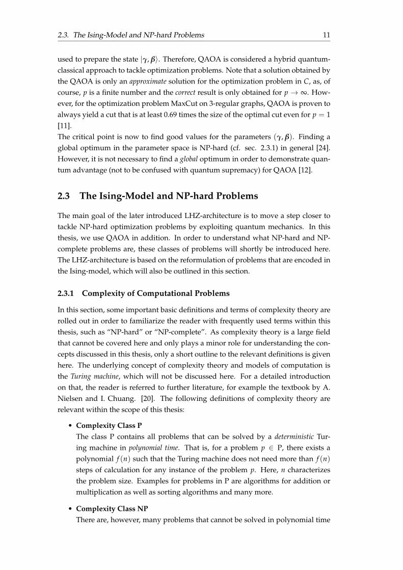
NP-hardNPC
FIGURE 2.1: The complexity classes in a Venn-Diagram.
by a deterministic Turing machine. Some of them can be solved in polynomialtime by a non-deterministic Turing machine. Non-deterministic in this contextimplies that the path of calculation is not uniquely determined. This suggeststhe definition of the complexity class NP which contains all problems that canbe solved in polynomial time by a non-deterministic Turing machine. Equiv-alently, NP can be defined as the set of all problems for which a deterministicTuring machine can decide if a solution candidate is indeed a solution, in poly-nomial time. This implies that P is a subset of NP, i. e. P ⊆ NP.
• A problem p is called NP-hard, if any problem in NP can be reduced to p inpolynomial time.
• A problem p is called NP-complete (NPC), if p is NP-hard and p ∈ NP. Exam-ples for NP-complete problems are Graph Partitioning, which will be discussedin detail in section 2.3.3, or the Traveling Salesman Problem.
An overview over these classes of problems is given in fig. 2.1, assuming thatP 6= NP. One of the most prominent unsolved problems in computer science isthe “P vs. NP problem” and asks whether or not P = NP. This is also one of the Mil-lennium Prize Problems [25].
There are many further complexity classes and relations between them, also con-cerning quantum computation in particular [20]. The interested reader might alsowant to refer to [26].
2.3.2 Ising Spin Glasses
The Ising model describing ferromagnetism in solid state physics was introduced byE. Ising in 1924 [27]. The Ising spin glass model for N spins is represented by theHamiltonian
H =N
∑i=1
∑j<i
Jijσ(i)z σ
(j)z +
N
∑i=1
hiσ(i)z . (2.32)
2.3. The Ising-Model and NP-hard Problems 13
G
(a) Initial situation for the optimizationproblem “Graph Partitioning”.
−→σi σi
σi σi
σi
σi
σiσi
G1 G2
(b) Solution for “Graph Partitioning”.
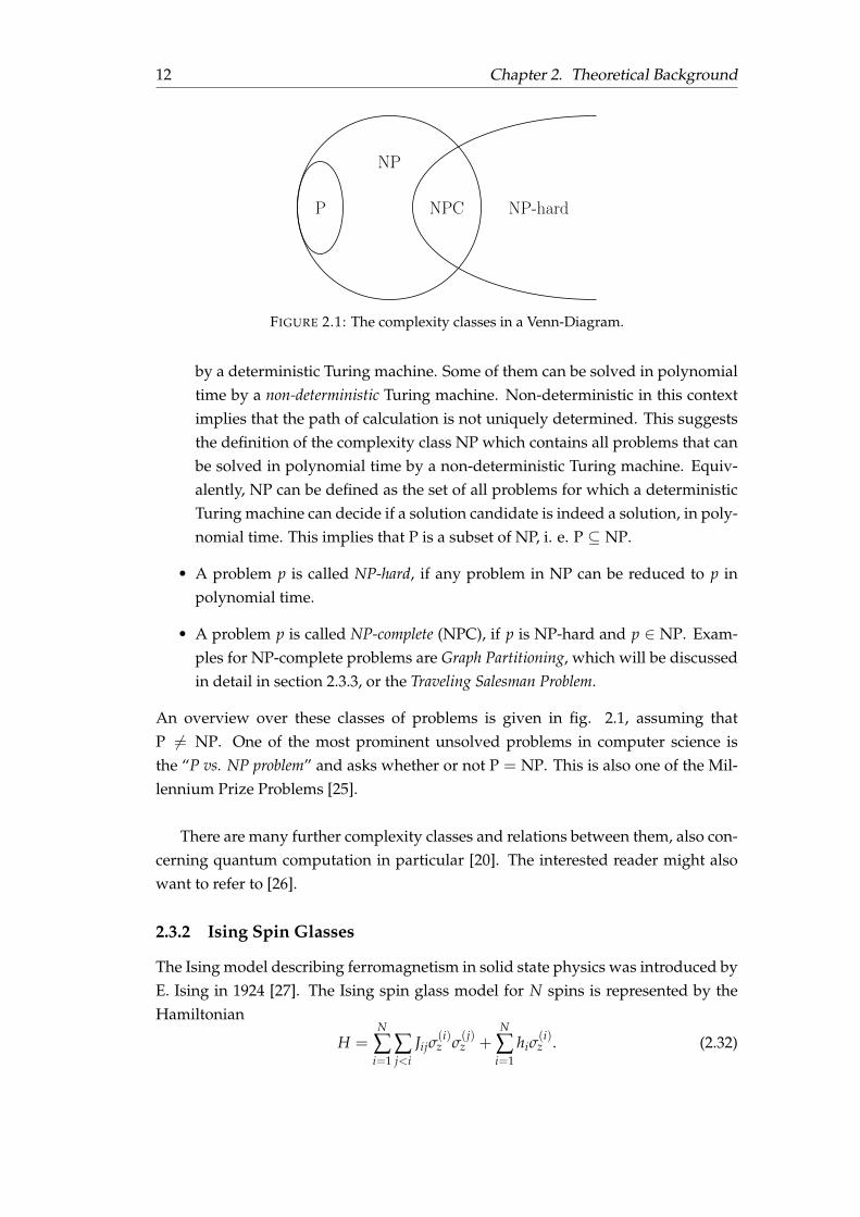
FIGURE 2.2: Illustrating the solution of “Graph Partitioning”. Thegraph is separated into two subgraphs G1 and G2 with equal size.In (b), green and red vertices correspond to σi = 1 and σi = −1,
respectively.
Here, σ(i)z denotes the z-Paulimatrix associated with the i-th spin. Formally, this
means thatσ(i)z = 1⊗ · · · ⊗ 1︸ ︷︷ ︸
(i−1) times
⊗σz ⊗ 1⊗ · · · ⊗ 1︸ ︷︷ ︸(N−i) times
. (2.33)
The matrix elements Jij of the interaction matrix J describe the interaction strengthbetween spin i and spin j. The interaction matrix is symmetric, i. e. Jij = Jji. Inaddition, the second term takes local magnetic fields hi into account. In general, thevalues Jij and hi can be positive or negative. This implies that, in contrast to a(n)(anti-)ferromagnetic structure, there is no magnetic ordering. A crucial point in thismodel is that there is an all-to-all interaction between the spins, i. e. there are not onlynext-neighbor interactions but each spin interacts with all other spins. Ising spinglasses are NP-hard problems [28]; so a relation of this model to other NP problemsis obvious. Indeed, due to the definitions of complexity classes discussed above,NP-complete optimization problems can be encoded within Ising spin glasses withpolynomial resources. A. Lucas gave a list of such problems in [7]. After encoding anoptimization problem in the spin glass formalism, finding its solution is equivalentto finding the ground state of the corresponding Spin-Glass Hamiltonian. One ex-ample for an NP-complete problem that can be formulated within an Ising model isthe problem of Graph Partitioning, which shall be discussed in the following section.
2.3.3 Example: Graph Partitioning
As an example of casting an optimization problem into a spin glass Hamiltonian, letus consider the problem of Graph Partitioning, which is also listed in [7]. Graph Par-titioning is known to be NP-complete and is the original example of a map betweenIsing spin glasses and NP-complete problems [29]. Consider a graph G consisting ofN vertices V connected by edges E (see fig. 2.2a). The goal is to split the graph intotwo subgraphs G1 and G2 with G = G1 ∪ G2, each containing N/2 vertices, such that
14 Chapter 2. Theoretical Background
the number of edges connecting the two subsets is minimized. Thus, a solution ofthe problem has to fulfill the two following conditions:
(i) The two subsets have the same size.
(ii) The number of vertices connecting them is minimal.
Now, we identify every vertex with a qubit σi = ±1, and declare
σi = +1⇐⇒ σi ∈ G1 and
σi = −1⇐⇒ σi ∈ G2,
as depicted in fig 2.2b. The values assigned to σi correspond to the possible mea-surement outcome when measuring σz defined in eq. (2.8). Having these relationsin mind, we can now define the Hamiltonians
HA = CA
(N
∑i=1
σi
)2
and HB = CB ∑i,j∈E
1− σiσj
2, (2.34)
in which CA,B define the weights of the conditions. In the following, we show thatminimizing HA and HB is equivalent to fulfilling condition (i) and (ii), respectively.Let us have a look at HA, initially. If the two subsets are of equal size, the sum ∑i σi iszero. Squaring it ensures that all other arrangements of σi lead to a higher value forthis term, no matter which subset contains more elements. Thus, finding the mini-mum of HA is equivalent to fulfilling the condition (i).
In order to understand that HB corresponds with condition (ii), consider theproduct σiσj. On the one hand, if σi and σj belong to the same subset, σiσj = +1holds and the corresponding term does not contribute to the total sum. On the otherhand, if they belong to different subsets, σiσj = −1 holds and the term contributesto the sum. Therefore, HB is minimal iff condition (ii) is fulfilled. The total ProblemHamiltonian is then
Hp = HA + HB = CA
(N
∑i=1
σi
)2
+ CB ∑i,j∈E
1− σiσj
2. (2.35)
From this definition it is obvious that the minimum energy of Hp is equivalentwith a solution of Graph Partitioning. By tuning the coefficients CA and CB, it canbe selected whether condition (i) or (ii) shall have higher priority. This form of theHamiltonian, as predicted, corresponds to the form of the Hamiltonian of the spinglass model (2.32). A more detailed description of the Ising formulation of this prob-lem and of many other optimization problems such as the Travelling Salesman prob-lem can be found in [7].
2.4. The LHZ-architecture 15
2.4 The LHZ-architecture
Although an important step has been made by encoding NP problems in the Isingmodel, one still encounters the problem of all-to-all connectivity in the Hamiltonian(2.32). To achieve a universal device to solve an arbitrary problem in the spin glassformalism, every single element of the interaction matrix Jij needs to be controllable.This makes it difficult to achieve universality by using the spin glass paradigm.
A promising approach that overcomes these difficulties, is the LHZ-architecturepresented by W. Lechner et. al. in 2015, which uses local interactions only by us-ing four-body interactions [8], originally developed for the purpose of quantum an-nealing. Although initially intended for quantum annealing, the LHZ-scheme alsoexhibits advantages for the implementation of QAOA [30] as will be shown in thefollowing chapters. The idea of this architecture will be outlined in this section. Fur-thermore, we will discuss how to translate NP-hard problems into the LHZ-schemeand exploit its advantages.
2.4.1 Translating the Spin-Glass Hamiltonian
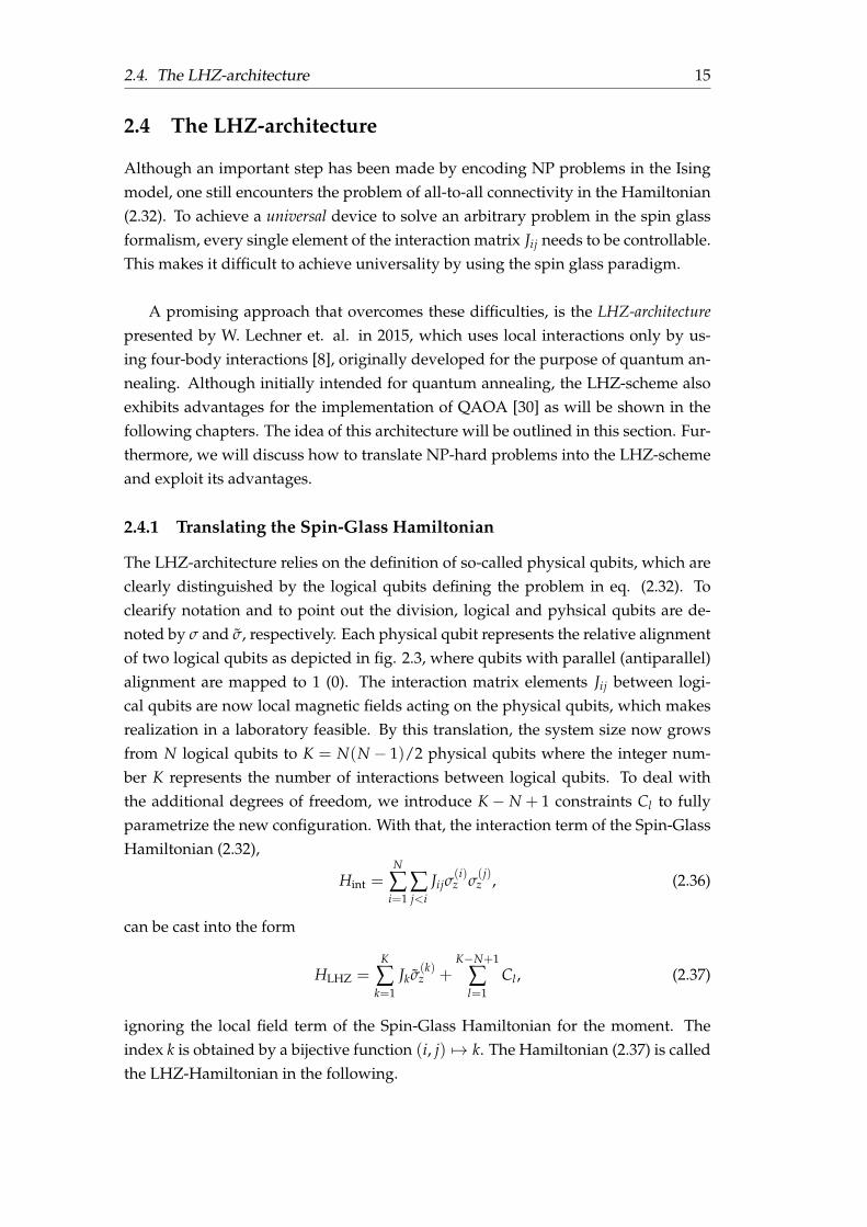
The LHZ-architecture relies on the definition of so-called physical qubits, which areclearly distinguished by the logical qubits defining the problem in eq. (2.32). Toclearify notation and to point out the division, logical and pyhsical qubits are de-noted by σ and σ, respectively. Each physical qubit represents the relative alignmentof two logical qubits as depicted in fig. 2.3, where qubits with parallel (antiparallel)alignment are mapped to 1 (0). The interaction matrix elements Jij between logi-cal qubits are now local magnetic fields acting on the physical qubits, which makesrealization in a laboratory feasible. By this translation, the system size now growsfrom N logical qubits to K = N(N − 1)/2 physical qubits where the integer num-ber K represents the number of interactions between logical qubits. To deal withthe additional degrees of freedom, we introduce K− N + 1 constraints Cl to fullyparametrize the new configuration. With that, the interaction term of the Spin-GlassHamiltonian (2.32),
Hint =N
∑i=1
∑j<i
Jijσ(i)z σ
(j)z , (2.36)
can be cast into the form
HLHZ =K
∑k=1
Jkσ(k)z +
K−N+1
∑l=1
Cl , (2.37)
ignoring the local field term of the Spin-Glass Hamiltonian for the moment. Theindex k is obtained by a bijective function (i, j) 7→ k. The Hamiltonian (2.37) is calledthe LHZ-Hamiltonian in the following.
16 Chapter 2. Theoretical Background
↑ ↑ 1= ↑ ↓ 0= ↓ ↑ 0= ↓ ↓ 1=
FIGURE 2.3: Conversion from logical qubits (blue) to physical qubits(green). The physical qubits represent the relative alignment of the
logical qubits.
↑1 ↓2 ↑3 ↑4 ↓5 ↑6
12
13
14
1516
23
24
25
26
34
35
36
45
46
56
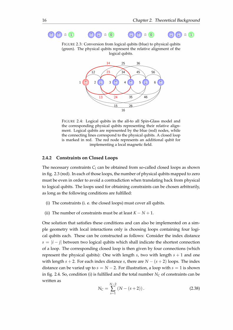
FIGURE 2.4: Logical qubits in the all-to all Spin-Glass model andthe corresponding physical qubits representing their relative align-ment. Logical qubits are represented by the blue (red) nodes, whilethe connecting lines correspond to the physical qubits. A closed loopis marked in red. The red node represents an additional qubit for
implementing a local magnetic field.
2.4.2 Constraints on Closed Loops
The necessary constraints Cl can be obtained from so-called closed loops as shownin fig. 2.3 (red). In each of those loops, the number of physical qubits mapped to zeromust be even in order to avoid a contradiction when translating back from physicalto logical qubits. The loops used for obtaining constraints can be chosen arbitrarily,as long as the following conditions are fulfilled:
(i) The constraints (i. e. the closed loops) must cover all qubits.
(ii) The number of constraints must be at least K− N + 1.
One solution that satisfies these conditions and can also be implemented on a sim-ple geometry with local interactions only is choosing loops containing four logi-cal qubits each. These can be constructed as follows: Consider the index distances = |i − j| between two logical qubits which shall indicate the shortest connectionof a loop. The corresponding closed loop is then given by four connections (whichrepresent the physical qubits): One with length s, two with length s + 1 and onewith length s + 2. For each index distance s, there are N − (s + 2) loops. The indexdistance can be varied up to s = N − 2. For illustration, a loop with s = 1 is shownin fig. 2.4. So, condition (i) is fulfilled and the total number NC of constraints can bewritten as
NC =N−2
∑s=1
(N − (s + 2)) . (2.38)
2.4. The LHZ-architecture 17
0
12
0
23
1
34
0
45
0
56
1
13
0
24
0
35
1
46
1
14
1
25
1
36
0
15
0
26
1
16
1 1 1 1
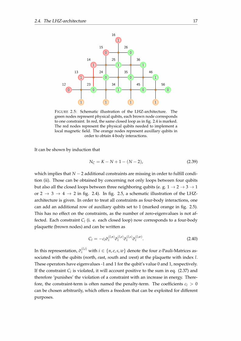
FIGURE 2.5: Schematic illustration of the LHZ-architecture. Thegreen nodes represent physical qubits, each brown node correspondsto one constraint. In red, the same closed loop as in fig. 2.4 is marked.The red nodes represent the physical qubits needed to implement alocal magnetic field. The orange nodes represent auxillary qubits in
order to obtain 4-body interactions.
It can be shown by induction that
NC = K− N + 1− (N − 2), (2.39)
which implies that N − 2 additional constraints are missing in order to fulfill condi-tion (ii). Those can be obtained by concerning not only loops between four qubitsbut also all the closed loops between three neighboring qubits (e. g. 1→ 2→ 3→ 1or 2 → 3 → 4 → 2 in fig. 2.4). In fig. 2.5, a schematic illustration of the LHZ-architecture is given. In order to treat all constraints as four-body interactions, onecan add an additional row of auxiliary qubits set to 1 (marked orange in fig. 2.5).This has no effect on the constraints, as the number of zero-eigenvalues is not af-fected. Each constraint Cl (i. e. each closed loop) now corresponds to a four-bodyplaquette (brown nodes) and can be written as
Cl = −cl σ(l,n)z σ
(l,e)z σ
(l,s)z σ
(l,w)z . (2.40)
In this representation, σ(l,i)z with i ∈ n, e, s, w denote the four z-Pauli-Matrices as-
sociated with the qubits (north, east, south and west) at the plaquette with index l.These operators have eigenvalues -1 and 1 for the qubit’s value 0 and 1, respectively.If the constraint Cl is violated, it will account positive to the sum in eq. (2.37) andtherefore ’punishes’ the violation of a constraint with an increase in energy. There-fore, the constraint-term is often named the penalty-term. The coefficients cl > 0can be chosen arbitrarily, which offers a freedom that can be exploited for differentpurposes.
18 Chapter 2. Theoretical Background
↑1 ↓2 ↑3 ↑4 ↓5 ↑6
1213
1415
16
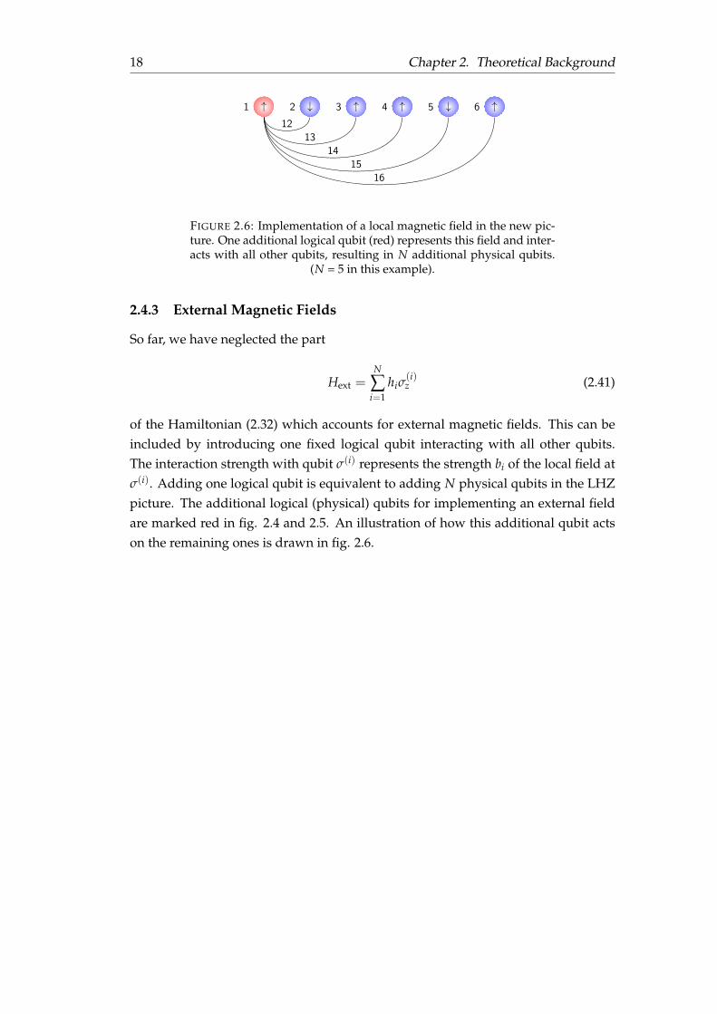
FIGURE 2.6: Implementation of a local magnetic field in the new pic-ture. One additional logical qubit (red) represents this field and inter-acts with all other qubits, resulting in N additional physical qubits.
(N = 5 in this example).
2.4.3 External Magnetic Fields
So far, we have neglected the part
Hext =N
∑i=1
hiσ(i)z (2.41)
of the Hamiltonian (2.32) which accounts for external magnetic fields. This can beincluded by introducing one fixed logical qubit interacting with all other qubits.The interaction strength with qubit σ(i) represents the strength bi of the local field atσ(i). Adding one logical qubit is equivalent to adding N physical qubits in the LHZpicture. The additional logical (physical) qubits for implementing an external fieldare marked red in fig. 2.4 and 2.5. An illustration of how this additional qubit actson the remaining ones is drawn in fig. 2.6.
19
Chapter 3
Embedding Strategies for theQAOA
Having now reviewed the important theoretical aspects, let us now have a look ondifferent strategies to solve an optimization problem encoded in an Ising spin glassby using QAOA. In this chapter, we will outline the problem we are considering andthen describe some possibilities to implement it.
3.1 The Problem to be implemented
3.1.1 Our Example: A 3-regular Graph
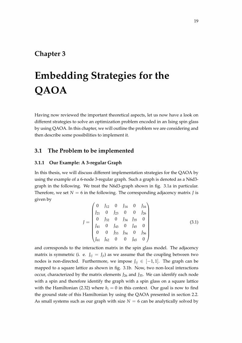
In this thesis, we will discuss different implementation strategies for the QAOA byusing the example of a 6-node 3-regular graph. Such a graph is denoted as a N6d3-graph in the following. We treat the N6d3-graph shown in fig. 3.1a in particular.Therefore, we set N = 6 in the following. The corresponding adjacency matrix J isgiven by
J =
0 J12 0 J14 0 J16
J21 0 J23 0 0 J26
0 J32 0 J34 J35 0J41 0 J43 0 J45 00 0 J53 J54 0 J56
J61 J62 0 0 J65 0
(3.1)
and corresponds to the interaction matrix in the spin glass model. The adjacencymatrix is symmetric (i. e. Jij = Jji) as we assume that the coupling between twonodes is non-directed. Furthermore, we impose Jij ∈ [−1, 1]. The graph can bemapped to a square lattice as shown in fig. 3.1b. Now, two non-local interactionsoccur, characterized by the matrix elements J26 and J35. We can idenfify each nodewith a spin and therefore identify the graph with a spin glass on a square latticewith the Hamiltonian (2.32) where hi = 0 in this context. Our goal is now to findthe ground state of this Hamiltonian by using the QAOA presented in section 2.2.As small systems such as our graph with size N = 6 can be analytically solved by
20 Chapter 3. Embedding Strategies for the QAOA
1
2
3
4
5
6
(a)
−→1 2
345
6
(b)
FIGURE 3.1: The 3-regular graph in fig. (a) is used as an example inthis thesis. Fig. (b) shows the mapping to a square lattice.
diagonalizing the Hamiltonian, we can quantify the quality of the solution by QAOAby comparing to the exact solution.
3.1.2 QAOA-Operators for our Problem
We will implement the QAOA algorithm for the interaction part of the spin glassHamiltonian (2.36) as well as for the LHZ-Hamiltonian (2.37). For the spin glass-Hamiltonian, the corresponding unitary operation is
Uint(γ) = e−iγHint =N
∏i=1
∏j<i
e−iγJijσ(i)z σ
(j)z , (3.2)
according to the definition of the QAOA-operator in eq. (2.26). Here, Jij denotes theadjacency matrix of the implemented graph as defined in eq. (3.1). Note that all theexponential terms commute. So, in a circuit, they can be arranged in an arbitraryorder. The mixing operator Ux is, in accordance with eq. (2.27),
Ux =N
∏j=1
e−iβσ(j)x . (3.3)
For implementing the LHZ-Hamiltonian in the spirit of QAOA, we need to set upthe unitary
ULHZ(γ) = e−iγHLHZ =K
∏k=1
e−iγJkσ(k)z ·
K−N+1
∏l=1
e−iγCl , (3.4)
where the interaction strengths Jk are obtained by a bijective map from Jij as de-scribed in section 2.4. Here, Cl denote the different constraints and correspondingLHZ-plaquettes, respectively. Note that the Cl operators contain four-body interac-tion terms. Eq. (3.4) is obtained by inserting HLHZ into eq. (2.26). In order to do theoptimization in the QAOA procedure more efficiently, we can split the ULHZ in twoparts [30], such that
ULHZ(γ, Ω) = Uz(γ)Uc(Ω) (3.5)
3.2. Implementation of Interactions 21
with
Uz(γ) =K
∏k=1
e−iγJkσ(k)z and (3.6)
Uc(Ω) =K−N+1
∏l=1
e−iΩclσ(l,n)z σ
(l,e)z σ
(l,s)z σ
(l,w)z . (3.7)
After splitting the phase-separating operator, we obtain p additional parameters Ωi
and can introduce another array Ω of angles with Ω = (Ω1, . . . , Ωn). This enlargesthe parameter space of the optimization problem from 2p to 3p parameters and en-ables us to extend the standard QAOA-optimization in order to obtain better resultsat lower QAOA-depths. The mixing operator Ux(β) for the LHZ-scheme is definedanalog to eq. (3.3) with the summation index running from 1 to K instead of N. Asdiscussed in section 2.4, the constraint coefficients cl can be arbitrarily chosen as longas they conserve the ground state. This makes it possible to treat them as QAOA-parameters as well and optimize them within the QAOA-scheme [30]. In order topreserve simplicity, this last step has not been done within this thesis.
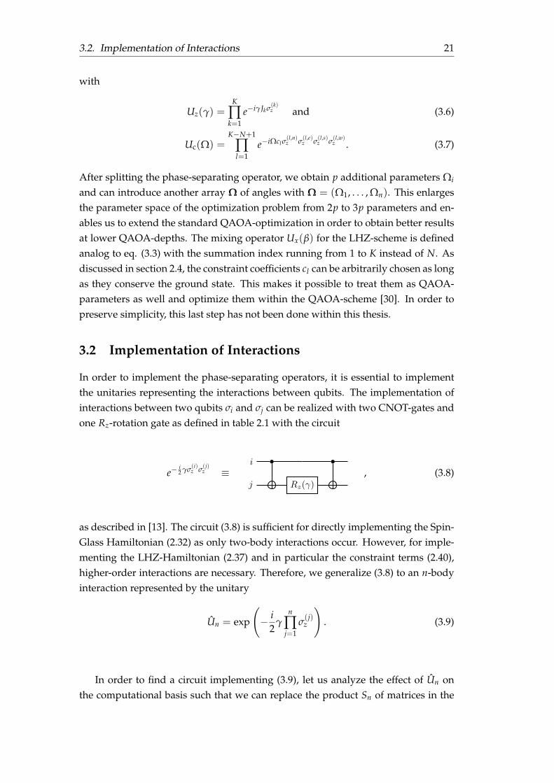
3.2 Implementation of Interactions
In order to implement the phase-separating operators, it is essential to implementthe unitaries representing the interactions between qubits. The implementation ofinteractions between two qubits σi and σj can be realized with two CNOT-gates andone Rz-rotation gate as defined in table 2.1 with the circuit
e−i2 γσ
(i)z σ
(j)z ≡
i
j Rz(γ), (3.8)
as described in [13]. The circuit (3.8) is sufficient for directly implementing the Spin-Glass Hamiltonian (2.32) as only two-body interactions occur. However, for imple-menting the LHZ-Hamiltonian (2.37) and in particular the constraint terms (2.40),higher-order interactions are necessary. Therefore, we generalize (3.8) to an n-bodyinteraction represented by the unitary
Un = exp
(− i
2γ
n
∏j=1
σ(j)z
). (3.9)
In order to find a circuit implementing (3.9), let us analyze the effect of Un onthe computational basis such that we can replace the product Sn of matrices in the
22 Chapter 3. Embedding Strategies for the QAOA
exponent by a product of eigenvalues si of σz with Sn = ∏nj=1 sj. Consider an ar-
bitrary basis state |k〉 = |k1k2 . . . kn〉. Here, ki ∈ 0, 1 denote the qubits involved inthe interaction. If there is an even number of qubits in state |0〉, we have Sn = 1,otherwise Sn = −1, as σz |0〉 = − |0〉 and σz |1〉 = |1〉. This means that
Sn =n
∏j=1
sj = (−1)⊕n
j=1 k j , (3.10)
where ⊕ denotes the addition modulo 2. Now, we have
Un = e−i2 γSn , (3.11)
yielding a phase of e±i2 γ, depending on the value of Sn. Note that CNOTc,z represents
the mapCNOTc,t : |kc, kt〉 7→ |kc, kc ⊕ kt〉 , (3.12)
where c and t denote the index of the control and target qubit, respectively. Further-more, Rz has the effect
R(j)z (γ) : |k1 . . . k j . . . kn〉 7→ e−(−1)kj i
2 γ |k1 . . . k j . . . kn〉 (3.13)
in the computational basis. The idea is now to set the value of the last qubit kn to thesum modulo 2 of all values ki by using CNOT-gates,
kn :=n⊕
j=1
k j, (3.14)
then apply an Rz-rotation on kn and finally undo the changes performed when im-plementing (3.14) by again applying CNOT-gates. That is, we collect the parity infor-mation of all qubits at one qubits, do an Rz rotation there and leave all other qubitsinvariant. In an informal way, the circuit implementing Un can be written as
Un =
[n−1
∏i=1
CNOTi,i+1
]R(n)
z (γ)
[n−1
∏i=1
CNOTn−i,n−i+1
]. (3.15)
This makes it obvious that for implementing an interaction between n qubits, 2(n− 1)CNOT-gates and one Rz-rotation are necessary. Eq. (3.8) implements U2 in this fash-ion. Note that the order of the qubits is irrelevant, as the Pauli matrices acting ondifferent qubits commute. This implies a freedom of choice on which qubit the Rz-rotation is performed. The case n = 4, which we will need in order to implement the
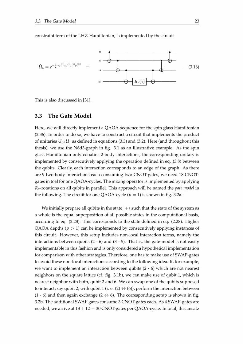
3.3. The Gate Model 23
constraint term of the LHZ-Hamiltonian, is implemented by the circuit
U4 = e−i2 γσ
(n)z σ
(e)z σ
(s)z σ
(w)z ≡
n
e
s
w Rz(γ)
. (3.16)
This is also discussed in [31].
3.3 The Gate Model
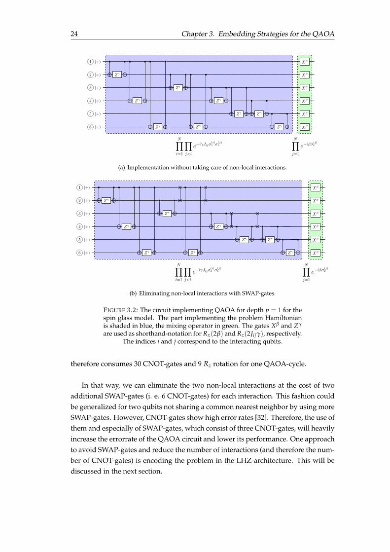
Here, we will directly implement a QAOA-sequence for the spin glass Hamiltonian(2.36). In order to do so, we have to construct a circuit that implements the productof unitaries UintUx as defined in equations (3.3) and (3.2). Here (and throughout thisthesis), we use the N6d3-graph in fig. 3.1 as an illustrative example. As the spinglass Hamiltonian only conatins 2-body interactions, the corresponding unitary isimplemented by consecutively applying the operation defined in eq. (3.8) betweenthe qubits. Clearly, each interaction corresponds to an edge of the graph. As thereare 9 two-body interactions each consuming two CNOT-gates, we need 18 CNOT-gates in toal for one QAOA-cycles. The mixing operator is implemented by applyingRx-rotations on all qubits in parallel. This approach will be named the gate model inthe following. The circuit for one QAOA-cycle (p = 1) is shown in fig. 3.2a.
We initially prepare all qubits in the state |+〉 such that the state of the system asa whole is the equal superposition of all possible states in the computational basis,according to eq. (2.28). This corresponds to the state defined in eq. (2.28). HigherQAOA depths (p > 1) can be implemented by consecutively applying instances ofthis circuit. However, this setup includes non-local interaction terms, namely theinteractions between qubits (2 - 6) and (3 - 5). That is, the gate model is not easilyimplementable in this fashion and is only considered a hypothetical implementationfor comparison with other strategies. Therefore, one has to make use of SWAP-gatesto avoid these non-local interactions according to the following idea. If, for example,we want to implement an interaction between qubits (2 - 6) which are not nearestneighbors on the square lattice (cf. fig. 3.1b), we can make use of qubit 1, which isnearest neighbor with both, qubit 2 and 6. We can swap one of the qubits supposedto interact, say qubit 2, with qubit 1 (i. e. (2)↔ (6)), perform the interaction between(1 - 6) and then again exchange (2 ↔ 6). The corresponding setup is shown in fig.3.2b. The additional SWAP gates consume 3 CNOT-gates each. As 4 SWAP-gates areneeded, we arrive at 18 + 12 = 30 CNOT-gates per QAOA-cycle. In total, this ansatz
24 Chapter 3. Embedding Strategies for the QAOA
N∏
i=1
∏
j<i
e−iγJijσ(i)z σ
(j)z
N∏
j=1
e−iβσ(j)x
1 |+〉 Xβ
2 |+〉 Zγ Xβ
3 |+〉 Zγ Xβ
4 |+〉 Zγ Zγ Xβ
5 |+〉 Zγ Zγ Xβ
6 |+〉 Zγ Zγ Zγ Xβ
(a) Implementation without taking care of non-local interactions.
N∏
i=1
∏
j<i
e−iγJijσ(i)z σ
(j)z
N∏
j=1
e−iβσ(j)x
1 |+〉 Xβ
2 |+〉 Zγ Xβ
3 |+〉 Zγ Xβ
4 |+〉 Zγ Zγ Xβ
5 |+〉 Zγ Zγ Xβ
6 |+〉 Zγ Zγ Zγ Xβ
(b) Eliminating non-local interactions with SWAP-gates.
FIGURE 3.2: The circuit implementing QAOA for depth p = 1 for thespin glass model. The part implementing the problem Hamiltonianis shaded in blue, the mixing operator in green. The gates Xβ and Zγ
are used as shorthand-notation for Rx(2β) and Rz(2Jijγ), respectively.The indices i and j correspond to the interacting qubits.
therefore consumes 30 CNOT-gates and 9 Rz rotation for one QAOA-cycle.
In that way, we can eliminate the two non-local interactions at the cost of twoadditional SWAP-gates (i. e. 6 CNOT-gates) for each interaction. This fashion couldbe generalized for two qubits not sharing a common nearest neighbor by using moreSWAP-gates. However, CNOT-gates show high error rates [32]. Therefore, the use ofthem and especially of SWAP-gates, which consist of three CNOT-gates, will heavilyincrease the errorrate of the QAOA circuit and lower its performance. One approachto avoid SWAP-gates and reduce the number of interactions (and therefore the num-ber of CNOT-gates) is encoding the problem in the LHZ-architecture. This will bediscussed in the next section.
3.4. LHZ-Proposal 25
3.4 LHZ-Proposal
In order to implement the graph in fig. 3.1 in the LHZ-scheme, we have to identifyphysical qubits and find constraints to compensate the enlargement of the Hilbert-space as described in sec. 2.4. We will see that the LHZ-scheme makes it possibleto save CNOT-gates. Furthermore, it enables us to implement QAOA on a squaredlattice, which is (when using K = N(N − 1)/2)) fully parallelizable [30]. These ad-vantages of LHZ and its implementation will be discussed in this section.
3.4.1 Finding Constraints and compiling the LHZ-scheme
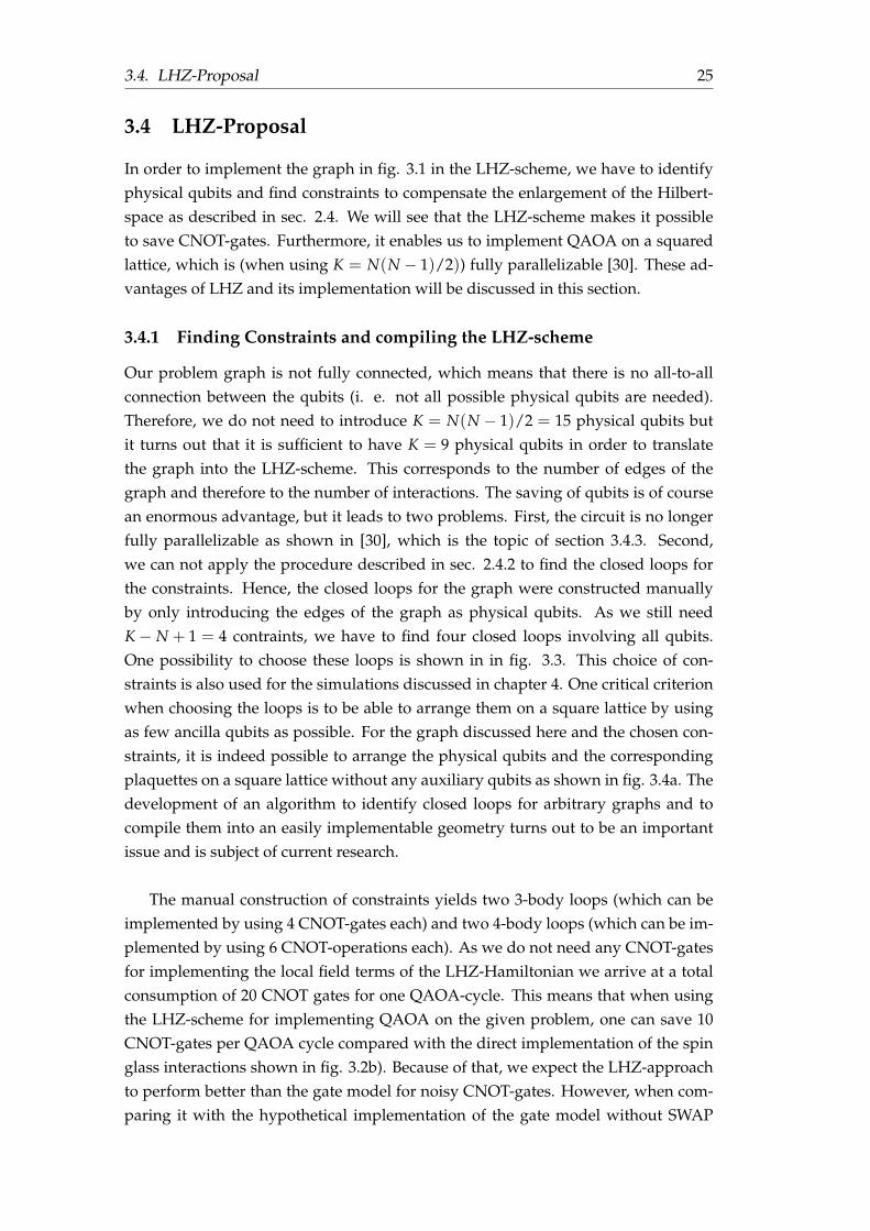
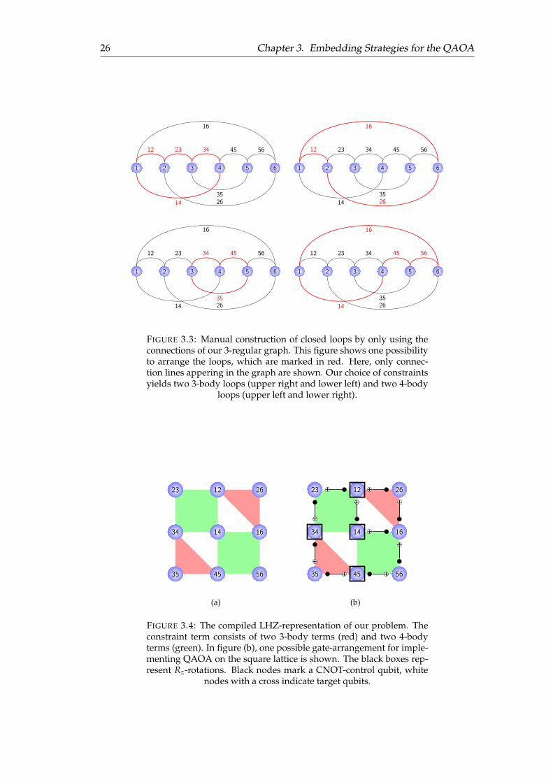
Our problem graph is not fully connected, which means that there is no all-to-allconnection between the qubits (i. e. not all possible physical qubits are needed).Therefore, we do not need to introduce K = N(N − 1)/2 = 15 physical qubits butit turns out that it is sufficient to have K = 9 physical qubits in order to translatethe graph into the LHZ-scheme. This corresponds to the number of edges of thegraph and therefore to the number of interactions. The saving of qubits is of coursean enormous advantage, but it leads to two problems. First, the circuit is no longerfully parallelizable as shown in [30], which is the topic of section 3.4.3. Second,we can not apply the procedure described in sec. 2.4.2 to find the closed loops forthe constraints. Hence, the closed loops for the graph were constructed manuallyby only introducing the edges of the graph as physical qubits. As we still needK− N + 1 = 4 contraints, we have to find four closed loops involving all qubits.One possibility to choose these loops is shown in in fig. 3.3. This choice of con-straints is also used for the simulations discussed in chapter 4. One critical criterionwhen choosing the loops is to be able to arrange them on a square lattice by usingas few ancilla qubits as possible. For the graph discussed here and the chosen con-straints, it is indeed possible to arrange the physical qubits and the correspondingplaquettes on a square lattice without any auxiliary qubits as shown in fig. 3.4a. Thedevelopment of an algorithm to identify closed loops for arbitrary graphs and tocompile them into an easily implementable geometry turns out to be an importantissue and is subject of current research.
The manual construction of constraints yields two 3-body loops (which can beimplemented by using 4 CNOT-gates each) and two 4-body loops (which can be im-plemented by using 6 CNOT-operations each). As we do not need any CNOT-gatesfor implementing the local field terms of the LHZ-Hamiltonian we arrive at a totalconsumption of 20 CNOT gates for one QAOA-cycle. This means that when usingthe LHZ-scheme for implementing QAOA on the given problem, one can save 10CNOT-gates per QAOA cycle compared with the direct implementation of the spinglass interactions shown in fig. 3.2b). Because of that, we expect the LHZ-approachto perform better than the gate model for noisy CNOT-gates. However, when com-paring it with the hypothetical implementation of the gate model without SWAP
26 Chapter 3. Embedding Strategies for the QAOA
1 2 3 4 5 6
12
14
16
23
26
34
35
45 56
1 2 3 4 5 6
12
14
16
23
26
34
35
45 56
1 2 3 4 5 6
12
14
16
23
26
34
35
45 56
1 2 3 4 5 6
12
14
16
23
26
34
35
45 56
FIGURE 3.3: Manual construction of closed loops by only using theconnections of our 3-regular graph. This figure shows one possibilityto arrange the loops, which are marked in red. Here, only connec-tion lines appering in the graph are shown. Our choice of constraintsyields two 3-body loops (upper right and lower left) and two 4-body
loops (upper left and lower right).
12 26
161434
23
35 45 56
(a)
12 26
161434
23
35 45 56
(b)
FIGURE 3.4: The compiled LHZ-representation of our problem. Theconstraint term consists of two 3-body terms (red) and two 4-bodyterms (green). In figure (b), one possible gate-arrangement for imple-menting QAOA on the square lattice is shown. The black boxes rep-resent Rz-rotations. Black nodes mark a CNOT-control qubit, white
nodes with a cross indicate target qubits.

3.4. LHZ-Proposal 27
gates (cf. fig. 3.2a), the LHZ-proposal consumes even two more CNOT gates despitethe fact that it is using more qubits. The advantage of LHZ, which will be shownin the next section, therefore originates from the non-local interactions that have tobe implemented when not translating the spin glass model to the LHZ scheme. Theimplementation of the local field term of the LHZ-Hamiltonian involves 9 parallelRz-rotations. Consequently, the number of Rz-gates per QAOA-cycle remains con-stant in comparison with the gate model.
3.4.2 Implementation of the Circuit on a Square Lattice
As discussed in the previous section, the closed constraint-loops for the problemwere cleverly chosen in a way such that the corresponding LHZ-plaquettes can bearranged on a square lattice as shown in fig. 3.4a. The interactions are now localizedon the plaquettes and can be implemented in the fashion shown in eq. (3.16). Thisis schematically depicted in fig. 3.4b, where the black squares around qubits respre-sent Rz-rotations. Also here, there are several possibilities to choose the location ofRz-rotations and CNOT-gates. This freedom of choice can be exploited to minimizethe number of „overlaps“ between different plaquettes arising when parallelizingthe circuit (cf. sec. 3.4.3). Here, the position of the Rz gates was chosen in a waysuch that there is only one rotation gate on a qubit (in the part implementing theconstraint part Uc of ULHZ), which can be seen in fig. 3.5, where the circuit imple-menting one QAOA-cycle is depicted. This has the advantage that the Rz-operationscan in principle be executed in parallel. These aspects will be examined in more de-tail in the next section. Another advantage of this setup on a square lattice is thereusability of CNOT-gates. When considering, for instance, the circuit in eq. (3.16),one needs only three physical CNOT-gates to implement it, because they can bereused in reversed order back after performing the Rz-operation [30].
As disussed in sec. 3.1.2, when implementing the QAOA in the LHZ-scheme,the sequence of unitary operations separates into three parts. Of course, we havethe mixing operator Ux, while the operator implementing the costfunction ULHZ canbe written as UzUc. This separation is also obvious in fig. 3.5, where Uz is shadedblue, Uc red and Ux is marked green. The operator Uz only involves Rz-rotations,while Uc is more complex and involves CNOT-gates. Therefore, Uc is the critical partwhen it comes to introducing noisy CNOT gates.
3.4.3 Parallelization of the LHZ-ansatz for QAOA
The idea of parallelizing the QAOA-procedure on the LHZ-architecture was givenby W. Lechner in 2018 [30] and makes use of the fact that the interactions on four-body plaquettes can be implemented by the circuits in eq. (3.16). The circuits (3.16)can all be implemented in parallel, such that all Rz-rotations take place at the same
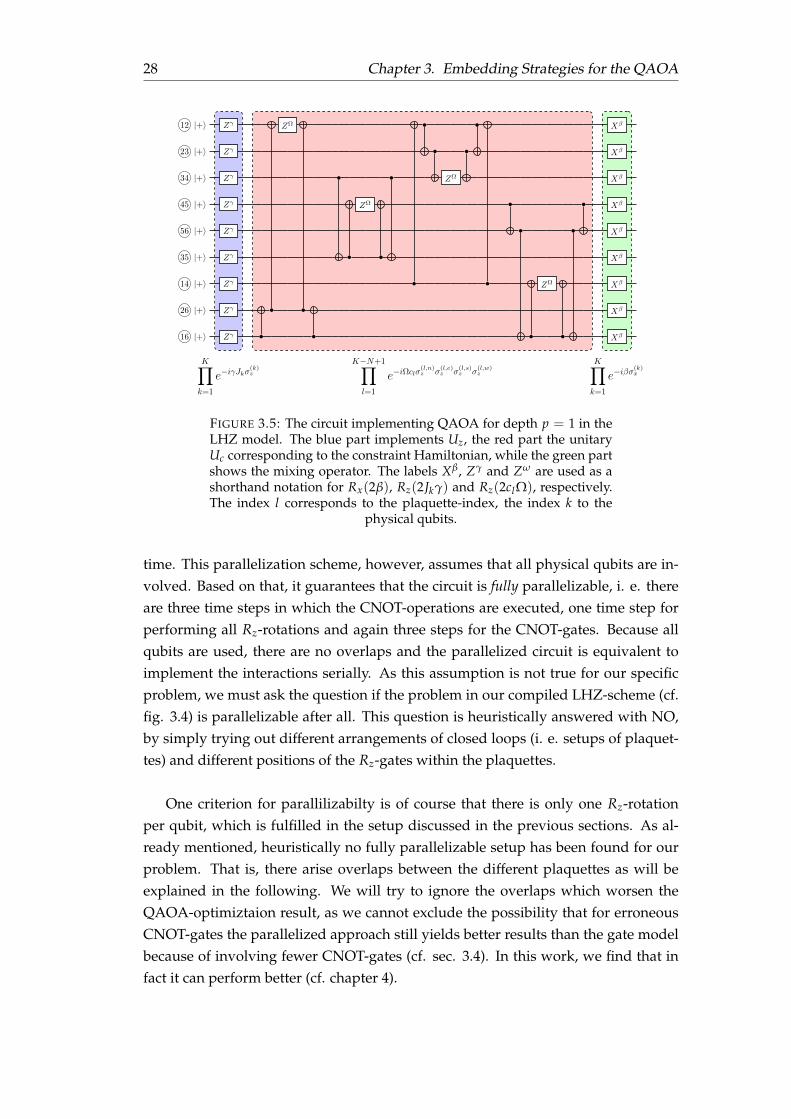
28 Chapter 3. Embedding Strategies for the QAOA
K∏
k=1
e−iγJkσ(k)z
K−N+1∏
l=1
e−iΩclσ(l,n)z σ
(l,e)z σ
(l,s)z σ
(l,w)z
K∏
k=1
e−iβσ(k)x
12 |+〉 Zγ ZΩ Xβ
23 |+〉 Zγ Xβ
34 |+〉 Zγ ZΩ Xβ
45 |+〉 Zγ ZΩ Xβ
56 |+〉 Zγ Xβ
35 |+〉 Zγ Xβ
14 |+〉 Zγ ZΩ Xβ
26 |+〉 Zγ Xβ
16 |+〉 Zγ Xβ
FIGURE 3.5: The circuit implementing QAOA for depth p = 1 in theLHZ model. The blue part implements Uz, the red part the unitaryUc corresponding to the constraint Hamiltonian, while the green partshows the mixing operator. The labels Xβ, Zγ and Zω are used as ashorthand notation for Rx(2β), Rz(2Jkγ) and Rz(2clΩ), respectively.The index l corresponds to the plaquette-index, the index k to the
physical qubits.
time. This parallelization scheme, however, assumes that all physical qubits are in-volved. Based on that, it guarantees that the circuit is fully parallelizable, i. e. thereare three time steps in which the CNOT-operations are executed, one time step forperforming all Rz-rotations and again three steps for the CNOT-gates. Because allqubits are used, there are no overlaps and the parallelized circuit is equivalent toimplement the interactions serially. As this assumption is not true for our specificproblem, we must ask the question if the problem in our compiled LHZ-scheme (cf.fig. 3.4) is parallelizable after all. This question is heuristically answered with NO,by simply trying out different arrangements of closed loops (i. e. setups of plaquet-tes) and different positions of the Rz-gates within the plaquettes.
One criterion for parallilizabilty is of course that there is only one Rz-rotationper qubit, which is fulfilled in the setup discussed in the previous sections. As al-ready mentioned, heuristically no fully parallelizable setup has been found for ourproblem. That is, there arise overlaps between the different plaquettes as will beexplained in the following. We will try to ignore the overlaps which worsen theQAOA-optimiztaion result, as we cannot exclude the possibility that for erroneousCNOT-gates the parallelized approach still yields better results than the gate modelbecause of involving fewer CNOT-gates (cf. sec. 3.4). In this work, we find that infact it can perform better (cf. chapter 4).
3.4. LHZ-Proposal 29
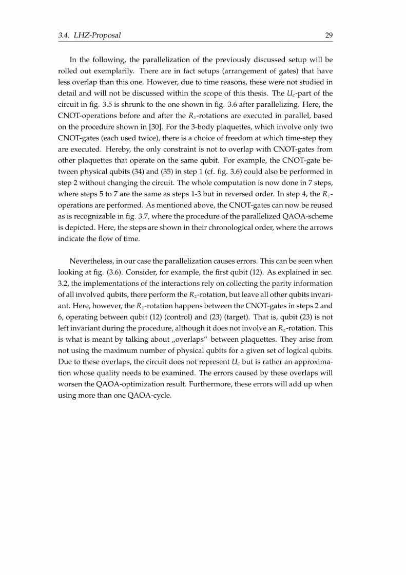
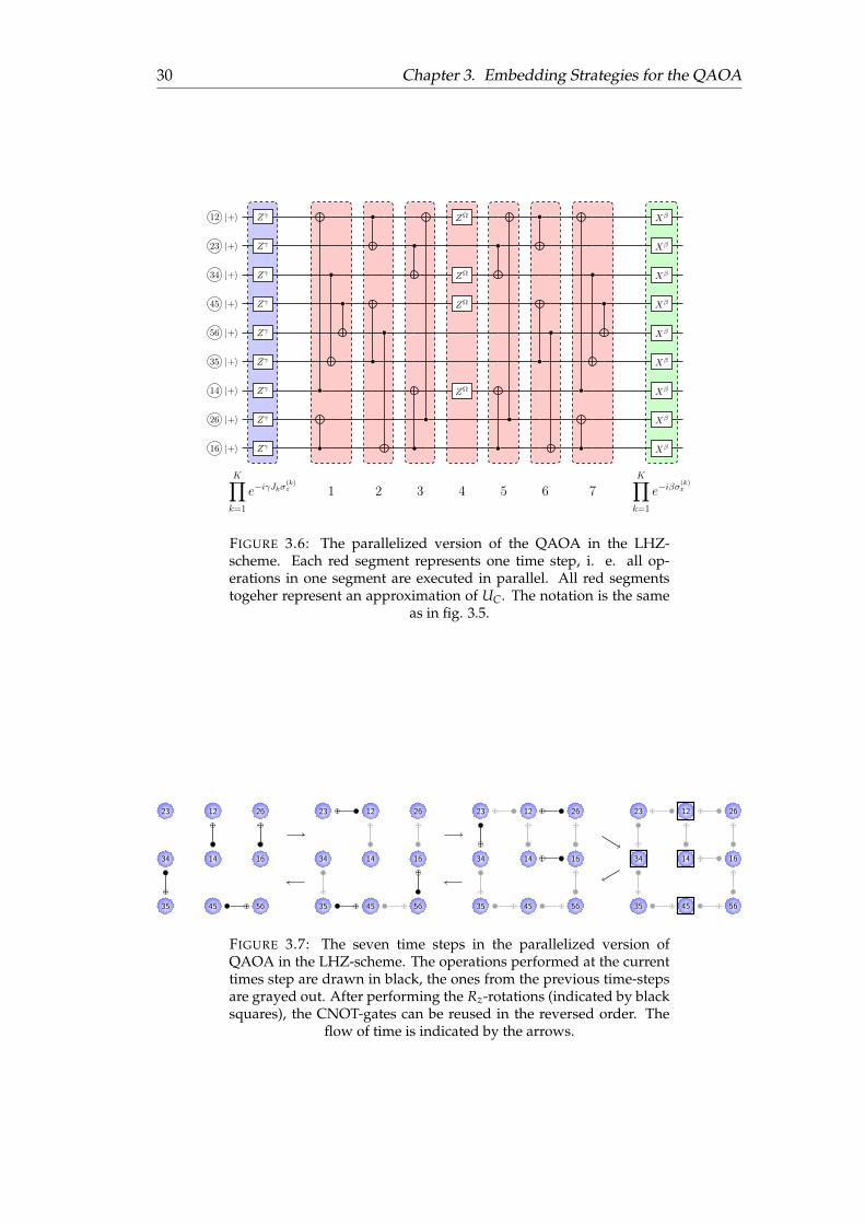
In the following, the parallelization of the previously discussed setup will berolled out exemplarily. There are in fact setups (arrangement of gates) that haveless overlap than this one. However, due to time reasons, these were not studied indetail and will not be discussed within the scope of this thesis. The Uc-part of thecircuit in fig. 3.5 is shrunk to the one shown in fig. 3.6 after parallelizing. Here, theCNOT-operations before and after the Rz-rotations are executed in parallel, basedon the procedure shown in [30]. For the 3-body plaquettes, which involve only twoCNOT-gates (each used twice), there is a choice of freedom at which time-step theyare executed. Hereby, the only constraint is not to overlap with CNOT-gates fromother plaquettes that operate on the same qubit. For example, the CNOT-gate be-tween physical qubits (34) and (35) in step 1 (cf. fig. 3.6) could also be performed instep 2 without changing the circuit. The whole computation is now done in 7 steps,where steps 5 to 7 are the same as steps 1-3 but in reversed order. In step 4, the Rz-operations are performed. As mentioned above, the CNOT-gates can now be reusedas is recognizable in fig. 3.7, where the procedure of the parallelized QAOA-schemeis depicted. Here, the steps are shown in their chronological order, where the arrowsindicate the flow of time.
Nevertheless, in our case the parallelization causes errors. This can be seen whenlooking at fig. (3.6). Consider, for example, the first qubit (12). As explained in sec.3.2, the implementations of the interactions rely on collecting the parity informationof all involved qubits, there perform the Rz-rotation, but leave all other qubits invari-ant. Here, however, the Rz-rotation happens between the CNOT-gates in steps 2 and6, operating between qubit (12) (control) and (23) (target). That is, qubit (23) is notleft invariant during the procedure, although it does not involve an Rz-rotation. Thisis what is meant by talking about „overlaps“ between plaquettes. They arise fromnot using the maximum number of physical qubits for a given set of logical qubits.Due to these overlaps, the circuit does not represent Uc but is rather an approxima-tion whose quality needs to be examined. The errors caused by these overlaps willworsen the QAOA-optimization result. Furthermore, these errors will add up whenusing more than one QAOA-cycle.
30 Chapter 3. Embedding Strategies for the QAOA
K∏
k=1
e−iγJkσ(k)z 1 2 3 4 5 6 7
K∏
k=1
e−iβσ(k)x
12 |+〉 Zγ ZΩ Xβ
23 |+〉 Zγ Xβ
34 |+〉 Zγ ZΩ Xβ
45 |+〉 Zγ ZΩ Xβ
56 |+〉 Zγ Xβ
35 |+〉 Zγ Xβ
14 |+〉 Zγ ZΩ Xβ
26 |+〉 Zγ Xβ
16 |+〉 Zγ Xβ
FIGURE 3.6: The parallelized version of the QAOA in the LHZ-scheme. Each red segment represents one time step, i. e. all op-erations in one segment are executed in parallel. All red segmentstogeher represent an approximation of UC. The notation is the same
as in fig. 3.5.
12 26
161434
23
35 45 56
12 26
161434
23
35 45 56
12 26
161434
23
35 45 56
12 26
161434
23
35 45 56
FIGURE 3.7: The seven time steps in the parallelized version ofQAOA in the LHZ-scheme. The operations performed at the currenttimes step are drawn in black, the ones from the previous time-stepsare grayed out. After performing the Rz-rotations (indicated by blacksquares), the CNOT-gates can be reused in the reversed order. The
flow of time is indicated by the arrows.
31
Chapter 4
Simulations and Results
In this work, the strategies for implementation of QAOA discussed in the previoussection are simulated by using the Python package cirq [17]. The details of theimplementation and the simulation results shall be discussed in this section. Weinvestigate the behavior of the different implementation schemes for different error-rates ε of CNOT-Gates and for different numbers p of QAOA-cycles. Furthermore,two different classical optimization routines are applied, which are also introducedin this section. We always do the optimization of the QAOA-parameters with respectto the ground state fidelity of the state ρ returned by the QAOA-routine, i. e. wefeed F(ρ, |φ0〉) to the classical optimizer. Here, |φ0〉 represents the ground state ofthe problem Hamiltonian. Note that the ground state can also be given by a set ofvectors due to degeneracy of the ground state energy as discussed in sec. 2.1.3.
4.1 Simulation Methods
For implementing the classical optimizer in QAOA as discussed in sec. 2.2, we usetwo different optimization algorithms in order to have a redundant validation ofour results. On the one hand, we apply the Nelder-Mead method (also called down-hill simplex method) [3] which is available in Python’s scipy.optimize package asa standard feature. On the other hand, we use the a stochastic, Metropolis-basedprocedure [2] relying on a Monte Carlo simulation which is implemented by hand.These two algorithms are briefly discussed in the following.
4.1.1 Metropolis Algorithm
The Metropolis algorithm was originally proposed by Nicholas Metropolis et. alin 1953 [2]. Its global parameter is the temperature T which is set at the beginning.Here, we use a variant for finding the minimum of a real function with N parameters
f :([0, 2π)
)N→ R : x = (x1 . . . xn) 7→ f (x). (4.1)
Here, the boundary of 2π has been chosen arbitrarily in view of the use for QAOA.The procedure is the following:
1. Initialize all parameters xi = 1 for all i with 1 ≤ i ≤ N.
32 Chapter 4. Simulations and Results
2. Introduce xopt which shall contain the point that minimizes f at the end of theoptimization routine. Set xopt := x.
3. Set y = (y1, . . . , yn) := x. Choose a random index i and update yi := yi, whereyi is randomly chosen from [0, 2π).
4. Evaluate f (x) and consider the following two cases:
(a) If f (y) ≤ f (x), accept the new configuration by setting x := y.
(b) Otherwise, if f (y) > f (x), follow the procedure below:
i. Calculate the probability pacc for accepting the new configuration al-though it yields a worse result according to
pacc = exp(− f (y)− f (x)
kBT
), (4.2)
where kB denotes the Boltzmann constant and is set to 1 here.
ii. Choose a random number 0 ≤ r ≤ 1. If r < pacc accept the configu-ration and set x = y. Otherwise, reject the new configuration and donothing.
5. Update the yet best solution, i. e. if f (x) < f (xopt), set xopt := x.
6. If some termination condition is fulfilled, return xopt. Otherwise, continue thealgorithm by returning to step 3.
For our purposes, we chose to terminate the optimization when a certain numberof iterations is reached. It is also possible to introduce convergence conditions andterminate when the result has not improved for a certain number of steps. In addi-tion, the procedure can be improved by reducing the temperature T monotonouslyduring the optimization. In that case, the procedure is called Simulated annealing [33].
When using the algorithm in the context of QAOA, the function f (x) corre-sponds to the costfunction of the optimization problem. The parameters x are identi-fied with the QAOA-parameters β and γ as defined in sec. 2.2. For the LHZ-scheme,also the parameters Ω (cf. sec. 3.1.2) are added, such that x = (β, γ, Ω). That is, ineach iteration, the update of one random QAOA-parameter is tried, similar to theoptimization procedure used in [30].
4.1.2 Nelder-Mead Algorithm
The Nelder-Mead method (or downhill-simplex method) is an algorithm for solvingnonlinear optimization problems with multiple parameters. It was presented by J.A. Nelder and R. Mead in 1965 [3]. Here, only the main idea of the algorithm shall bediscussed. The goal is to minimize a function f : RN → R, where N is the numberof parameters. The following steps summarize the procedure given in [3] and arebased on [34] and simplified.
4.1. Simulation Methods 33
1. Initialization. Start by randomly choosing N + 1 points xi ∈ RN , 1 ≤ i ≤ N,which span an N-dimensional simplex. In two dimensions, this correspondsto a triangle, in three dimensions to a tetrahedron. As discussed in sec. 4.1.1,in the context of QAOA, the points xi correspond to the QAOA-parameters.
2. Ordering. Sort these points by their function value such that
f (x1) ≤ · · · ≤ f (xN) ≤ f (xN+1). (4.3)
3. Check Termination Condition. Check whether the terminating condition is ful-filled. If so, stop the iteration and return the result x1.
4. Average the points xi apart from the worst point xN+1. The result correspondsto the centroid x of the simplex spanned by these points.
5. Reflection. Reflect xN+1 at the centroid x. The newly obtained point shall be
xr = x + α · (x− xN+1) (4.4)
with α > 0.
6. Expansion. If xr is better than xN+1 (which means that f (xr) < f (xN+1)), calcu-late
xe = x + β · (xr − x) (4.5)
with β > 1. If xe is better than xr, set xN+1 := xe, else set xN+1 := xr.
7. Outside contraction. If xN is better than xr and xr is better than xN+1, calculate
xoc = x + γ · (xr − x) (4.6)
with γ ∈ (0, 0.5]. If xoc is better than xr, set xN+1 := xc. Otherwise go to step 9.
8. Inside contraction. If xr is better than xN+1, compute
xic = x− γ · (xr − x) (4.7)
with γ ∈ (0, 1). If xic is better than xN+1, set xN+1 = xic.
9. Shrinking. Replace all points apart from the best one (which is x1) by setting
xi := x1 + δ · (xi − x1) for 1 < i ≤ N + 1, (4.8)
where δ ∈ (0, 1) and go to step 2.
Still, some criteria for the termination of the procedure must be found. Thiscan be done by setting a limit for the number of iterations or setting a „minimumsize“ for the simplex, which is not deceeded [34]. The Nelder-Mead method works
34 Chapter 4. Simulations and Results
very well for low-dimensional problems. However, it may become more and moreineffective with increasing dimension, as discussed, for example, in [35]. There areimproved algorithms that are able to tackle these problems (for instance [36]), butthese will not be used within this thesis. For further reading on the Nelder-Meadalgorithm, also see [37].
4.2 General Framework
Here, we discuss the setup for our simulation. We introduce the cirq-package andexplain the noise model used in the simulations. Also, the parameters used for thesimulations can be found in this section.
4.2.1 The cirq-Package
The cirq package is a Pythion library for „writing, manipulating an optimizing quan-tum ciruits and running them against quantum computers and simulators“ [17] and waspresented at the International Workshop on Quantum Software and Quantum Ma-chine Learning in 2018. It enables the user to setup arbitrary quantum circuits andsimulate them. An advantage we made use of is that cirq is capable of tracking thequantum state |ψ〉 of the system throughout the circuit until the end. That is, we cansave resources as we do not need to do the sampling of measurement results in step2 in chapter 2.2 in order to obtain a good estimate of an expectation value. Instead,we obtain the desired expectation value of an observable by evaluating eq. (2.6).Even if quantum noise is involved, we can do the same simulation using densitymatrices, i. e. we can do exact simulations even for noisy circuits. In that case weevolve a density matrix ρ through the circuit and calculate e. g. the energy expecta-tion according to eq. (2.5). The same holds for calculating the ground state fidelityof the state obtained by the QAOA, which will be our quantity of interest.
It might seem more efficient to calculate with pure sates instead of density ma-trices and sample a sufficiently large number of trials. However, that turned out tobe more time-consuming than doing the evolution through the circuit for the wholedensity matrix. Therefore, we used density matrices instead of sampling multipleruns.
4.2.2 Noise-model for the Simulations
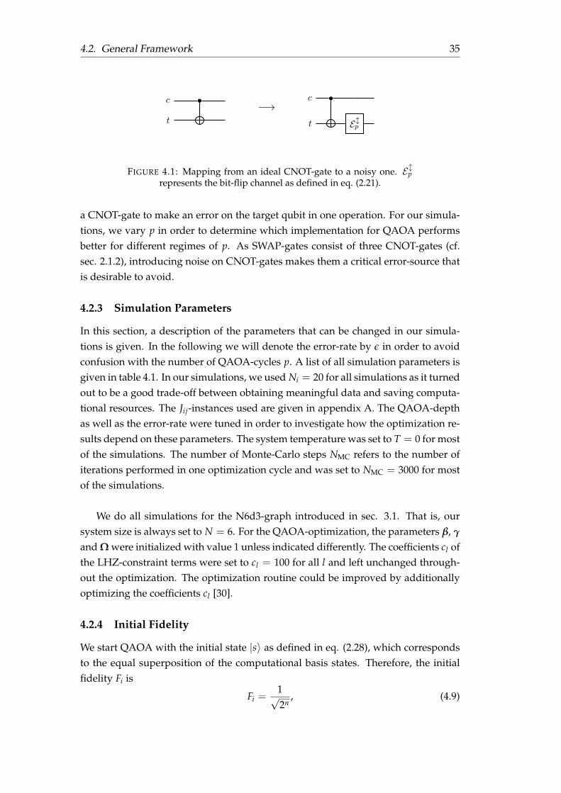
Concerning the types of quantum noise, we restrict ourselves to bit-flip noise onCNOT-gates in this thesis. Within this model, we assume CNOT-gates to be erro-neous and model that by performing a bit-flip on the gate’s target qubit with proba-bility p after the CNOT-operation has been performed. In order to do so, we use thebit-flip channel as defined in eq. (2.21). The mapping from an ideal CNOT-gate to anerroneous one is depicted in fig. 4.1. The errorrate p represents the probability for
4.2. General Framework 35
c
t
−→c
t Elp
FIGURE 4.1: Mapping from an ideal CNOT-gate to a noisy one. Elprepresents the bit-flip channel as defined in eq. (2.21).
a CNOT-gate to make an error on the target qubit in one operation. For our simula-tions, we vary p in order to determine which implementation for QAOA performsbetter for different regimes of p. As SWAP-gates consist of three CNOT-gates (cf.sec. 2.1.2), introducing noise on CNOT-gates makes them a critical error-source thatis desirable to avoid.
4.2.3 Simulation Parameters
In this section, a description of the parameters that can be changed in our simula-tions is given. In the following we will denote the error-rate by ε in order to avoidconfusion with the number of QAOA-cycles p. A list of all simulation parameters isgiven in table 4.1. In our simulations, we used Ni = 20 for all simulations as it turnedout to be a good trade-off between obtaining meaningful data and saving computa-tional resources. The Jij-instances used are given in appendix A. The QAOA-depthas well as the error-rate were tuned in order to investigate how the optimization re-sults depend on these parameters. The system temperature was set to T = 0 for mostof the simulations. The number of Monte-Carlo steps NMC refers to the number ofiterations performed in one optimization cycle and was set to NMC = 3000 for mostof the simulations.
We do all simulations for the N6d3-graph introduced in sec. 3.1. That is, oursystem size is always set to N = 6. For the QAOA-optimization, the parameters β, γ
and Ω were initialized with value 1 unless indicated differently. The coefficients cl ofthe LHZ-constraint terms were set to cl = 100 for all l and left unchanged through-out the optimization. The optimization routine could be improved by additionallyoptimizing the coefficients cl [30].
4.2.4 Initial Fidelity
We start QAOA with the initial state |s〉 as defined in eq. (2.28), which correspondsto the equal superposition of the computational basis states. Therefore, the initialfidelity Fi is
Fi =1√2n
, (4.9)
36 Chapter 4. Simulations and Results
Parameter Symbol Remarks
System size N Corresponds to the number of logical qubits in-volved in the optimization problem
Circuit depth p Corresponds to the number of QAOA-cycles
Error-rate ε The probability for a CNOT-gate to produce anerroneous result in one operation
Number of instances Ni The number of instances averaged over
Number of MC-steps NMC only for the Metropolis-optimization
System temperature T only for the Metropolis-optimization
Constraint strength cl Strength of the LHZ-constraints as defined ineq. (2.40)
TABLE 4.1: List of simulation parameters.
where n denotes the number of qubits used. In the gate model, we use 6 qubits forthe N6d3-graph, which would lead to
Fi =1√26
=1√64
=18
. (4.10)
However, the ground state of the Ising spin glass Hamiltonian (which is used in thegate model) is twice degenerate. Due to that degeneracy, the initial fidelity must becalculated according to formula (2.17) or (2.16) for a pure or mixed state, respectively,and increases to
F(g)i =
1√2n−1
=1√32≈ 0.177. (4.11)
Here F(g)i denotes the initial fidelity in the gate model. In the LHZ-scheme, we use 9
qubits and the degeneracy is lifted. Therefore, the initial fidelity for the N6d3-graphin the LHZ-scheme F(LHZ)
i is
F(LHZ)i =
1√29
=1√512≈ 0.044. (4.12)
The initial fidelities will play an important role when comparing the different ap-proaches for QAOA implementation. As they are the starting point for the opti-mization procedure, they act a lower bound for the final fidelity result. Furthermore,the fact that the fidelity of the equal-superposition state is much lower for the LHZ-model implies that a state with fidelity F in the LHZ-scheme might contain moreinformation about the true ground state than a state with the same fidelity in thegate model. For example, if F = F(g)
i for both models, we cannot extract any infor-mation about the true ground state from the output state in the gate model (as thefidelity it is not more than for the superposition state). However, in the LHZ-scheme,one can tell the output state is closer to the true ground state than the input state.
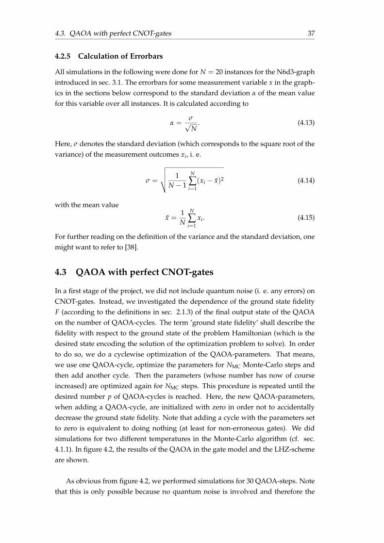
4.3. QAOA with perfect CNOT-gates 37
4.2.5 Calculation of Errorbars
All simulations in the following were done for N = 20 instances for the N6d3-graphintroduced in sec. 3.1. The errorbars for some measurement variable x in the graph-ics in the sections below correspond to the standard deviation α of the mean valuefor this variable over all instances. It is calculated according to
α =σ√N
. (4.13)
Here, σ denotes the standard deviation (which corresponds to the square root of thevariance) of the measurement outcomes xi, i. e.
σ =
√√√√ 1N − 1
N
∑i=1
(xi − x)2 (4.14)
with the mean value
x =1N
N
∑i=1
xi. (4.15)
For further reading on the definition of the variance and the standard deviation, onemight want to refer to [38].
4.3 QAOA with perfect CNOT-gates
In a first stage of the project, we did not include quantum noise (i. e. any errors) onCNOT-gates. Instead, we investigated the dependence of the ground state fidelityF (according to the definitions in sec. 2.1.3) of the final output state of the QAOAon the number of QAOA-cycles. The term ’ground state fidelity’ shall describe thefidelity with respect to the ground state of the problem Hamiltonian (which is thedesired state encoding the solution of the optimization problem to solve). In orderto do so, we do a cyclewise optimization of the QAOA-parameters. That means,we use one QAOA-cycle, optimize the parameters for NMC Monte-Carlo steps andthen add another cycle. Then the parameters (whose number has now of courseincreased) are optimized again for NMC steps. This procedure is repeated until thedesired number p of QAOA-cycles is reached. Here, the new QAOA-parameters,when adding a QAOA-cycle, are initialized with zero in order not to accidentallydecrease the ground state fidelity. Note that adding a cycle with the parameters setto zero is equivalent to doing nothing (at least for non-erroneous gates). We didsimulations for two different temperatures in the Monte-Carlo algorithm (cf. sec.4.1.1). In figure 4.2, the results of the QAOA in the gate model and the LHZ-schemeare shown.
As obvious from figure 4.2, we performed simulations for 30 QAOA-steps. Notethat this is only possible because no quantum noise is involved and therefore the
38 Chapter 4. Simulations and Results
0 5 10 15 20 25 30p
0.2
0.3
0.4
0.5
0.6
0.7
0.8
0.9
1.0
F
Gate ModelLHZ
(a) T = 0.00.
0 5 10 15 20 25 30p
0.2
0.3
0.4
0.5
0.6
0.7
0.8
0.9
1.0
F
Gate ModelLHZ
(b) T = 0.02.
FIGURE 4.2: Depencence of the ground state fidelity F on the num-ber of QAOA-cycles for perfect CNOT-gates. For each QAOA-cycle,5000 Monte-Carlo steps were performed. In fig. (a) a temperature ofT = 0.00 was used for the Metropolis algorithm while we set T = 0.02
in fig. (b). The results were averaged over 20 instances.
use of density matrices is not necessary. For noisy gates, only up to 10 QAOA-cycles were used (cf. sec 4.4). As expected, the ground state fidelity increasesmonotonously with the number of QAOA cycles.
However, we can make an interesting observation when comparing the resultsfor the different Monte-Carlo temperatures. For low-depth QAOA (i. e. low p),the algorithm performs better at zero temperature for both implementation strate-gies. Nevertheless, as p increases, the algorithm yields better results for T = 0.02.One possible explanation for this behaviour is that for more QAOA-cycles also thenumber of the parameters to optimize (i. e. the search space) increases. We as-sume that the Monte-Carlo routine gets stuck more easily in local minima in a largersearch space for zero tepmerature. We also find that for non-erroneous CNOT-gates,the gate model performs better than the LHZ-scheme. This can be attributed to thelarger search space for the LHZ-model (as the number of parameters here is 3p in-stead of 2p) and the larger number of qubits.
4.4 QAOA with imperfect (noisy) CNOT-gates
Having obtained a feeling of how the number of QAOA-cycles changes the perfor-mance of the optimization for an ideal circuit, we now introduce quantum noise. Wewill see that the behaviour will significantly change. That indicates that it is impor-tant to take effects of quantum noise into account when implementing QAOA.

4.4. QAOA with imperfect (noisy) CNOT-gates 39
2 4 6 8 10p
0.3
0.4
0.5
0.6
0.7F
Gate ModelLHZ
(a) ε = 0.001.
2 4 6 8 10p
0.25
0.30
0.35
0.40
0.45
0.50
F
Gate ModelLHZ
(b) ε = 0.005.
2 4 6 8 10p
0.20
0.25
0.30
0.35
0.40
0.45
F
Gate ModelLHZ
(c) ε = 0.010.
2 4 6 8 10p
0.10
0.15
0.20
0.25
0.30
0.35
FGate ModelLHZ
(d) ε = 0.030.
FIGURE 4.3: Depencence of the ground state fidelity F on the numberof QAOA-cycles p for noisy CNOT-gates for different error-rates ε.For each QAOA-cycle, 1000 Monte-Carlo steps were performed. Thesystem temperature was set T = 0.02. If the LHZ-scheme performsbetter than the gate model or not depends on ε and p. Note thatthe scales are set individually for each image for better visibility and
therefore not comparable.
4.4.1 Fidelity vs. QAOA depth
When we introduce erroneous CNOT-gates as discussed in section 4.2.2, the behav-ior of the fidelity F under changing the number p of the QAOA cycles is no longermonotonous, as discussed in the previous section. In order to account for the quan-tum noise, we now have to involve density matrices in the simulation, which isresource-intensive. Therefore, we performed simulations only up to 10 QAOA cy-cles and only with 1000 Monte-Carlo-steps per QAOA-cycle. For the system tem-perature, we used T = 0.02. The results for T = 0.00 qualitatively coincide with thedata presented here. We chose to discuss the case T = 0.02 here as it seemed to bemore illustrative. Apart from that, we performed the same procedure as describedin sec. 4.3. In fig. 4.3, the dependence of F on p is shown for different error-rates ε.
40 Chapter 4. Simulations and Results
The simulation results show that there are regimes for which the LHZ-schemeyields higher ground state fidelities than the gate model. This behaviour has beenexpected since the LHZ-scheme involves less erroneous CNOT-gates as the gatemodel, as discussed in chapter 2. At first appearance, however, it seems counter-intuitive that the performance of QAOA can decrease while increasing the numberof QAOA-cycles. This can be explained by the fact that there is a trade-off betweenimproving the procedure by increasing p versus introducing more erroneous CNOT-gates by doing so. As a result, an optimal number popt(ε) depending on the error-rate ε and the implementation scheme can be extracted from the simulation resultsdepicted in fig. 4.3. It is obvious from the simulation results and intuitive (but notproven) that popt decreases for increasing ε. For increasing p, the difference betweenthe number of CNOT-gates in the gate model and in the LHZ-scheme also increases,which yields to a threshold in p for the LHZ-scheme to perform better. For ε = 0.005,this threshold is at p = 8 (cf. fig. 4.3b), for ε = 0.01, it is at p = 6 (cf. fig. 4.3c).
It seems plausible that for larger ε, the threshold for the LHZ-scheme to performbetter decreases as well as popt, as a change of ε has a larger impact on the gate modeldue to the larger number of CNOT-gates. What is not obvious, however, is that forlarger error-rates (e. g. ε = 0.03), there is no crossing-point of the fidelity-curves andthe gate model always performs better. We conjecture that this behavior is due to thefact that the fidelity is already close to F(g)
i , i. e. the ground-state fidelity for the gatemodel does not decrease as fast as it does for regimes where the fidelity is higher. AsF(LHZ)
i is significantly smaller, according to our assumption, this effect does not havesuch a massive impact on the LHZ-model.
4.4.2 Fidelity vs. Error-rate
In fig. 4.4, results of the same simulation as in sec. 4.4.1 are shown. Here, the fi-delity is depicted in dependence of the error-rate at fixed p. For p = 10 (cf. fig. 4.4b),the performance in the LHZ-scheme can exceed the performance in the gate model,while for p = 6 (cf. fig. 4.4a), it cannot. This also illustrates that there is a thresholdin p for the LHZ-model to be able to exceed the gate model.
The feature that the performance of the LHZ-implementation exceeds the gatemodel for a certain regime of error-rates is even more prominent if we do not opti-mize the QAOA-parameters in the cyclewise fashion as we did above but take intoaccount all parameters ab initio. The results depicted in fig. 4.5a were obtainedby optimizing the parameters for p = 10 and NMC = 3000. Furthermore, we setT = 0.00. In fig. 4.5b, the same simulation was performed by using the Nelder-Mead method instead of the Metropolis algorithm. As the results presented in fig.4.5 are considered to be the main result of this work, this additional simulation wasdone to verify the simulation outcome, and especially that the LHZ-scheme really
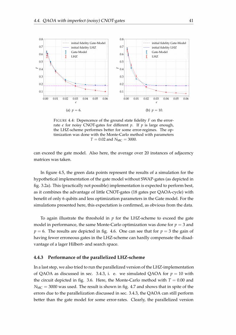
4.4. QAOA with imperfect (noisy) CNOT-gates 41
0.00 0.01 0.02 0.03 0.04 0.05 0.06ε
0.1
0.2
0.3
0.4
0.5
0.6
0.7
0.8F
initial fidelity Gate-Modelinitial fidelity LHZGate-ModelLHZ
(a) p = 6.
0.00 0.01 0.02 0.03 0.04 0.05 0.06ε
0.1
0.2
0.3
0.4
0.5
0.6
0.7
0.8
F
initial fidelity Gate-Modelinitial fidelity LHZGate-ModelLHZ
(b) p = 10.
FIGURE 4.4: Depencence of the ground state fidelity F on the error-rate ε for noisy CNOT-gates for different p. If p is large enough,the LHZ-scheme performes better for some error-regimes. The op-timization was done with the Monte-Carlo method with parameters
T = 0.02 and NMC = 3000.
can exceed the gate model. Also here, the average over 20 instances of adjacencymatrices was taken.
In figure 4.5, the green data points represent the results of a simulation for thehypothetical implementation of the gate model without SWAP-gates (as depicted infig. 3.2a). This (practically not possible) implementation is expected to perform best,as it combines the advantage of little CNOT-gates (18 gates per QAOA-cycle) withbenefit of only 6 qubits and less optimization parameters in the Gate model. For thesimulations presented here, this expectation is confirmed, as obvious from the data.
To again illustrate the threshold in p for the LHZ-scheme to exceed the gatemodel in performance, the same Monte-Carlo optimization was done for p = 3 andp = 6. The results are depicted in fig. 4.6. One can see that for p = 3 the gain ofhaving fewer erroneous gates in the LHZ-scheme can hardly compensate the disad-vantage of a lager Hilbert- and search space.
4.4.3 Performance of the parallelized LHZ-scheme
In a last step, we also tried to run the parallelized version of the LHZ-implementationof QAOA as discussed in sec. 3.4.3, i. e. we simulated QAOA for p = 10 withthe circuit depicted in fig. 3.6. Here, the Monte-Carlo method with T = 0.00 andNMC = 3000 was used. The result is shown in fig. 4.7 and shows that in spite of theerrors due to the parallelization discussed in sec. 3.4.3, the QAOA can still performbetter than the gate model for some error-rates. Clearly, the parallelized version
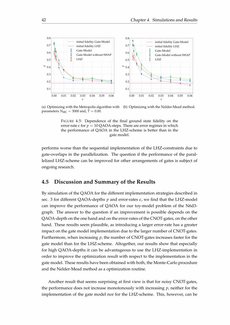
42 Chapter 4. Simulations and Results
0.00 0.01 0.02 0.03 0.04 0.05 0.06ε
0.1
0.2
0.3
0.4
0.5
0.6
0.7
0.8
Finitial fidelity Gate-Modelinitial fidelity LHZGate-ModelGate-Model without SWAPLHZ
(a) Optimizing with the Metropolis algorithm withparameters NMC = 3000 and, T = 0.00.
0.00 0.01 0.02 0.03 0.04 0.05 0.06ε
0.1
0.2
0.3
0.4
0.5
0.6
0.7
0.8
F
initial fidelity Gate-Modelinitial fidelity LHZGate-ModelGate-Model without SWAPLHZ
(b) Optimizing with the Nelder-Mead method.
FIGURE 4.5: Dependence of the final ground state fidelity on theerror-rate ε for p = 10 QAOA-steps. There are error regimes in whichthe performance of QAOA in the LHZ-scheme is better than in the
gate model.
performs worse than the sequential implementation of the LHZ-constraints due togate-overlaps in the parallelization. The question if the performance of the paral-lelized LHZ-scheme can be improved for other arrangements of gates is subject ofongoing research.
4.5 Discussion and Summary of the Results
By simulation of the QAOA for the different implementation strategies described insec. 3 for different QAOA-depths p and error-rates ε, we find that the LHZ-modelcan improve the performance of QAOA for our toy-model problem of the N6d3-graph. The answer to the question if an improvement is possible depends on theQAOA-depth on the one hand and on the error-rates of the CNOT-gates, on the otherhand. These results seem plausible, as introducing a larger error-rate has a greaterimpact on the gate model implementation due to the larger number of CNOT-gates.Furthermore, when increasing p, the number of CNOT-gates increases faster for thegate model than for the LHZ-scheme. Altogether, our results show that especiallyfor high QAOA-depths it can be advantageous to use the LHZ-implementation inorder to improve the optimization result with respect to the implementation in thegate model. These results have been obtained with both, the Monte-Carlo procedureand the Nelder-Mead method as a optimization routine.
Another result that seems surprising at first view is that for noisy CNOT-gates,the performance does not increase monotonously with increasing p, neither for theimplementation of the gate model nor for the LHZ-scheme. This, however, can be
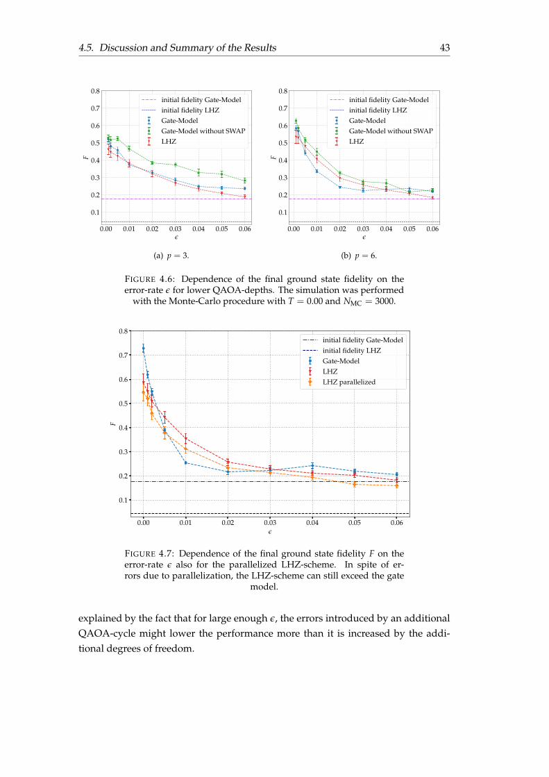
4.5. Discussion and Summary of the Results 43
0.00 0.01 0.02 0.03 0.04 0.05 0.06ε
0.1
0.2
0.3
0.4
0.5
0.6
0.7
0.8F
initial fidelity Gate-Modelinitial fidelity LHZGate-ModelGate-Model without SWAPLHZ
(a) p = 3.
0.00 0.01 0.02 0.03 0.04 0.05 0.06ε
0.1
0.2
0.3
0.4
0.5
0.6
0.7
0.8
F
initial fidelity Gate-Modelinitial fidelity LHZGate-ModelGate-Model without SWAPLHZ
(b) p = 6.
FIGURE 4.6: Dependence of the final ground state fidelity on theerror-rate ε for lower QAOA-depths. The simulation was performed
with the Monte-Carlo procedure with T = 0.00 and NMC = 3000.
0.00 0.01 0.02 0.03 0.04 0.05 0.06ε
0.1
0.2
0.3
0.4
0.5
0.6
0.7
0.8
F
initial fidelity Gate-Modelinitial fidelity LHZGate-ModelLHZLHZ parallelized
FIGURE 4.7: Dependence of the final ground state fidelity F on theerror-rate ε also for the parallelized LHZ-scheme. In spite of er-rors due to parallelization, the LHZ-scheme can still exceed the gate
model.
explained by the fact that for large enough ε, the errors introduced by an additionalQAOA-cycle might lower the performance more than it is increased by the addi-tional degrees of freedom.
44 Chapter 4. Simulations and Results
The results of the simulation for perfect CNOT-gates presented in sec. 4.3 indi-cate that for the Monte-Carlo method as a classical optimization routine, the perfor-mance of QAOA can be improved by choosing the system temperature accordingto the QAOA-depth. The question if there is a deeper relation between p and theoptimal system temperature has not been examined within the scope of this thesis.
The performance of QAOA in the parallelized version of the LHZ-scheme hasonly been examined marginally in this work. Nevertheless, the results suggest thata performance enhancement with respect to the gate model can also be achievedwith the parallelized LHZ-scheme. This seems to hold although the parallelizationintroduces additional faults in the quantum circuit as discussed in sec. 3.4.3.
45
Chapter 5
Outlook and Conclusion
To sum up, we have shown that for noisy CNOT-gates, the implementation of QAOAin the LHZ-scheme can be advantageous, especially for high QAOA-depths. Ourresults suggest that also the parallelization of the circuit in the LHZ-scheme canperform better than the standard gate model. That is, there is a trade-off betweenusing more qubits in the LHZ-scheme versus using more CNOT-gates in the gatemodel as soon as quantum noise is introduced. As the parallelization has only beenmarginally investigated within this thesis, it remains an open question whether theparallel setup can be optimized (e. g. by rearranging gates) in order to obtain evenbetter results.
Furthermore, it remains an open question how the suggested implementationstrategies perform for other instances of N6d3-graphs (i. e. for other connections be-tween the graph nodes). For the answer to that question, we presume results similarto the findings presented here. However, a question for further research is how theembedding strategies scale for larger graphs.
In addition, it is known that the initial values of the QAOA-parameters for theoptimization can have an impact on the quality of the solution of the optimizationproblem. Therefore, we suppose that the performance of the techniques presentedcan be improved by cleverly choosing the initial values. In order to do so, one coulde. g. try to find patterns in the space of QAOA-parameters. For that, also ideasof machine learning might be exploited. It is already a known fact that there areanalogies to Quantum Annealing when considering the optimal initial values forthe parameters [12].
Another possibility to improve the performance in the LHZ-scheme is to viewthe coefficients of the constraint-Hamiltonian as another set of QAOA-parametersand also optimize them in the QAOA procedure. This has already been suggested in[30]. For the Monte-Carlo optimization, one could apply more advanced techniquessuch as Simulated Annealing [33]. As discussed in sec. 4.5, one could investigateif the optimal system temperature for the Monte-Carlo procedure changes with theQAOA-depth.
46 Chapter 5. Outlook and Conclusion
Moreover, we have only considered quantum noise on CNOT-gates. It remainsan open question that may be treated in future research what impact errors on Rz-rotations would have on the performance of the different embedding schemes. Aswell as that, one could apply other noise models such as dephasing- or depolarizingchannels. Another point is that the circuits presented in sec. 3 are not unique. There-fore, rearrangement of gates might lead to an improvement (or also a degradiation)of the optimization result. The examination of these effects might also be a futureresearch topic.
Finally, in our simulations, we have only optimized the QAOA-parameters withrespect to the ground state fidelity. In practice, of course, this is not possible asthe desired ground state (which is necessary to calculate the fidelity) is not known.Therefore, one would always do an optimization with respect to the energy of theoutput state. How the different embedding strategies perform for these more prac-tical conditions has also not been examined here and is an important question forfurther research.
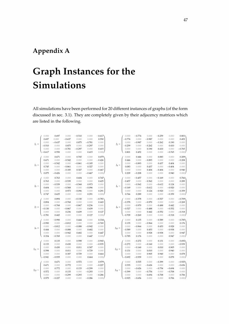
47
Appendix A
Graph Instances for theSimulations
All simulations have been performed for 20 different instances of graphs (of the formdiscussed in sec. 3.1). They are completely given by their adjacency matrices whichare listed in the following.
J1 =
0.000 0.697 0.000 −0.510 0.000 −0.6170.697 0.000 −0.637 0.000 0.000 0.5500.000 −0.637 0.000 0.875 −0.781 0.000−0.510 0.000 0.875 0.000 −0.297 0.000
0.000 0.000 −0.781 −0.297 0.000 0.415−0.617 0.550 0.000 0.000 0.415 0.000
J2 =
0.000 −0.774 0.000 −0.259 0.000 0.801−0.774 0.000 −0.987 0.000 0.000 0.452
0.000 −0.987 0.000 −0.262 0.190 0.000−0.259 0.000 −0.262 0.000 0.410 0.000
0.000 0.000 0.190 0.410 0.000 −0.7650.801 0.452 0.000 0.000 −0.765 0.000
J3 =
0.000 0.671 0.000 0.745 0.000 0.0750.671 0.000 −0.542 0.000 0.000 −0.4260.000 −0.542 0.000 −0.861 −0.185 0.0000.745 0.000 −0.861 0.000 0.327 0.0000.000 0.000 −0.185 0.327 0.000 −0.4670.075 −0.426 0.000 0.000 −0.467 0.000
J4 =
0.000 0.446 0.000 0.083 0.000 0.2090.446 0.000 −0.893 0.000 0.000 −0.2080.000 −0.893 0.000 0.437 0.404 0.0000.083 0.000 0.437 0.000 −0.404 0.0000.000 0.000 0.404 −0.404 0.000 0.9400.209 −0.208 0.000 0.000 0.940 0.000
J5 =
0.000 0.763 0.000 0.604 0.000 0.7470.763 0.000 −0.539 0.000 0.000 0.6250.000 −0.539 0.000 −0.568 0.973 0.0000.604 0.000 −0.568 0.000 −0.096 0.0000.000 0.000 0.973 −0.096 0.000 0.2910.747 0.625 0.000 0.000 0.291 0.000
J6 =
0.000 −0.457 0.000 −0.169 0.000 0.766−0.457 0.000 −0.562 0.000 0.000 0.289
0.000 −0.562 0.000 −0.612 0.124 0.000−0.169 0.000 −0.612 0.000 −0.920 0.000
0.000 0.000 0.124 −0.920 0.000 −0.3590.766 0.289 0.000 0.000 −0.359 0.000
J7 =
0.000 0.894 0.000 −0.130 0.000 −0.7810.894 0.000 −0.768 0.000 0.000 0.4430.000 −0.768 0.000 −0.867 0.236 0.000−0.130 0.000 −0.867 0.000 0.439 0.000
0.000 0.000 0.236 0.439 0.000 0.127−0.781 0.443 0.000 0.000 0.127 0.000
J8 =
0.000 −0.378 0.000 −0.527 0.000 −0.709−0.378 0.000 −0.970 0.000 0.000 −0.269
0.000 −0.970 0.000 −0.488 0.442 0.000−0.527 0.000 −0.488 0.000 −0.552 0.000
0.000 0.000 0.442 −0.552 0.000 −0.318−0.709 −0.269 0.000 0.000 −0.318 0.000
J9 =
0.000 −0.990 0.000 0.444 0.000 0.334−0.990 0.000 −0.812 0.000 0.000 −0.769
0.000 −0.812 0.000 −0.088 −0.942 0.0000.444 0.000 −0.088 0.000 0.682 0.0000.000 0.000 −0.942 0.682 0.000 0.4470.334 −0.769 0.000 0.000 0.447 0.000
J10 =
0.000 0.135 0.000 −0.589 0.000 −0.7850.135 0.000 −0.964 0.000 0.000 0.1760.000 −0.964 0.000 0.453 0.928 0.000−0.589 0.000 0.453 0.000 −0.938 0.000
0.000 0.000 0.928 −0.938 0.000 0.947−0.785 0.176 0.000 0.000 0.947 0.000
J11 =
0.000 0.133 0.000 0.598 0.000 −0.9410.133 0.000 0.430 0.000 0.000 −0.9350.000 0.430 0.000 0.011 0.307 0.0000.598 0.000 0.011 0.000 0.729 0.0000.000 0.000 0.307 0.729 0.000 0.664−0.941 −0.935 0.000 0.000 0.664 0.000
J12 =
0.000 −0.272 0.000 0.131 0.000 −0.692−0.272 0.000 −0.160 0.000 0.000 −0.939
0.000 −0.160 0.000 0.010 0.905 0.0000.131 0.000 0.010 0.000 0.940 0.0000.000 0.000 0.905 0.940 0.000 0.078−0.692 −0.939 0.000 0.000 0.078 0.000
J13 =
0.000 0.671 0.000 0.572 0.000 0.9790.671 0.000 0.772 0.000 0.000 −0.2270.000 0.772 0.000 0.133 −0.299 0.0000.572 0.000 0.133 0.000 −0.293 0.0000.000 0.000 −0.299 −0.293 0.000 −0.2860.979 −0.227 0.000 0.000 −0.286 0.000
J14 =
0.000 0.535 0.000 −0.399 0.000 −0.9250.535 0.000 −0.626 0.000 0.000 −0.6560.000 −0.626 0.000 −0.754 −0.694 0.000−0.399 0.000 −0.754 0.000 −0.708 0.000
0.000 0.000 −0.694 −0.708 0.000 0.706−0.925 −0.656 0.000 0.000 0.706 0.000
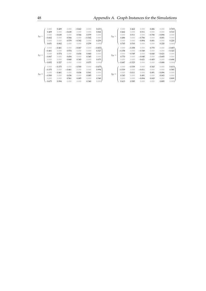
48 Appendix A. Graph Instances for the Simulations
J15 =
0.000 0.409 0.000 −0.662 0.000 0.6310.409 0.000 −0.630 0.000 0.000 0.0620.000 −0.630 0.000 0.544 0.579 0.000−0.662 0.000 0.544 0.000 −0.302 0.000
0.000 0.000 0.579 −0.302 0.000 0.2590.631 0.062 0.000 0.000 0.259 0.000
J16 =
0.000 0.462 0.000 0.486 0.000 0.7650.462 0.000 0.511 0.000 0.000 0.5100.000 0.511 0.000 −0.706 −0.894 0.0000.486 0.000 −0.706 0.000 0.001 0.0000.000 0.000 −0.894 0.001 0.000 0.2200.765 0.510 0.000 0.000 0.220 0.000
J17 =
0.000 −0.461 0.000 −0.067 0.000 −0.832−0.461 0.000 0.574 0.000 0.000 0.327
0.000 0.574 0.000 0.454 0.840 0.000−0.067 0.000 0.454 0.000 0.345 0.000
0.000 0.000 0.840 0.345 0.000 0.075−0.832 0.327 0.000 0.000 0.075 0.000
J18 =
0.000 −0.358 0.000 0.770 0.000 −0.687−0.358 0.000 −0.549 0.000 0.000 −0.323
0.000 −0.549 0.000 −0.040 −0.621 0.0000.770 0.000 −0.040 0.000 −0.405 0.0000.000 0.000 −0.621 −0.405 0.000 −0.684−0.687 −0.323 0.000 0.000 −0.684 0.000
J19 =
0.000 −0.375 0.000 −0.500 0.000 −0.675−0.375 0.000 −0.461 0.000 0.000 0.994
0.000 −0.461 0.000 0.036 0.561 0.000−0.500 0.000 0.036 0.000 0.085 0.000
0.000 0.000 0.561 0.085 0.000 0.340−0.675 0.994 0.000 0.000 0.340 0.000
J20 =
0.000 −0.539 0.000 0.343 0.000 0.413−0.539 0.000 −0.011 0.000 0.000 0.585
0.000 −0.011 0.000 0.491 −0.094 0.0000.343 0.000 0.491 0.000 0.043 0.0000.000 0.000 −0.094 0.043 0.000 0.8090.413 0.585 0.000 0.000 0.809 0.000
49
Bibliography
[1] S. Behera, S. Sahoo, and B. B. Pati. “A review on optimization algorithms andapplication to wind energy integration to grid”. In: Renewable and SustainableEnergy Reviews 48 (2015), pp. 214 –227. ISSN: 1364-0321. DOI: https://doi.org/10.1016/j.rser.2015.03.066. URL: http://www.sciencedirect.com/science/article/pii/S1364032115002191.
[2] N. Metropolis et al. “Equation of State Calculations by Fast Computing Ma-chines”. In: The Journal of Chemical Physics 21.6 (1953), pp. 1087–1092. DOI:10.1063/1.1699114. eprint: https://doi.org/10.1063/1.1699114. URL:https://doi.org/10.1063/1.1699114.
[3] J. A. Nelder and R. Mead. “A Simplex Method for Function Minimization”. In:The Computer Journal 7.4 (1965), pp. 308–313. DOI: 10.1093/comjnl/7.4.308.eprint: /oup/backfile/content_public/journal/comjnl/7/4/10.1093/comjnl/7.4.308/2/7- 4- 308.pdf. URL: http://dx.doi.org/10.1093/comjnl/7.4.308.
[4] T. Kadowaki and H. Nishimori. “Quantum Annealing in the Transverse IsingModel”. In: 58 (Apr. 1998).
[5] E. Farhi et al. “Quantum Computation by Adiabatic Evolution”. In: eprintarXiv:quant-ph/0001106 (Jan. 2000). eprint: quant-ph/0001106.
[6] M. Born and V. Fock. “Beweis des Adiabatensatzes”. In: Zeitschrift für Physik51.3 (Mar. 1928), pp. 165–180. ISSN: 0044-3328. DOI: 10.1007/BF01343193. URL:https://doi.org/10.1007/BF01343193.
[7] A. Lucas. “Ising formulations of many NP problems”. In: Frontiers in Physics2 (2014), p. 5. ISSN: 2296-424X. DOI: 10.3389/fphy.2014.00005. URL: https://www.frontiersin.org/article/10.3389/fphy.2014.00005.
[8] W. Lechner, P. Hauke, and P. Zoller. “A quantum annealing architecture withall-to-all connectivity from local interactions”. In: Science Advances 1.9 (2015).DOI: 10.1126/sciadv.1500838. eprint: http://advances.sciencemag.org/content/1/9/e1500838.full.pdf. URL: http://advances.sciencemag.org/content/1/9/e1500838.
[9] T. Albash, W. Vinci, and D. A. Lidar. “Simulated-quantum-annealing compari-son between all-to-all connectivity schemes”. In: Phys. Rev. A 94 (2 Aug. 2016),p. 022327. DOI: 10.1103/PhysRevA.94.022327. URL: https://link.aps.org/doi/10.1103/PhysRevA.94.022327.
50 Bibliography
[10] Y. Susa and H. Nishimori. “Performance Enhancement of Quantum Annealingunder the Lechner–Hauke–Zoller Scheme by Non-linear Driving of the Con-straint Term”. In: Journal of the Physical Society of Japan 89.4 (2020), p. 044006.DOI: 10.7566/JPSJ.89.044006. eprint: https://doi.org/10.7566/JPSJ.89.044006. URL: https://doi.org/10.7566/JPSJ.89.044006.
[11] E. Farhi, J. Goldstone, and S. Gutmann. A Quantum Approximate OptimizationAlgorithm. 2014. arXiv: 1411.4028 [quant-ph].
[12] L. Zhou et al. “Quantum Approximate Optimization Algorithm: Performance,Mechanism, and Implementation on Near-Term Devices.” In: arXiv: QuantumPhysics (2018).
[13] G. E. Crooks. Performance of the Quantum Approximate Optimization Algorithmon the Maximum Cut Problem. 2018. arXiv: 1811.08419 [quant-ph].
[14] J. D. Hunter. “Matplotlib: A 2D graphics environment”. In: Computing in Sci-ence & Engineering 9.3 (2007), pp. 90–95. DOI: 10.1109/MCSE.2007.55.
[15] T. Tantau. The TikZ and PGF Packages. Manual for version 3.0.0. Dec. 20, 2013.URL: http://sourceforge.net/projects/pgf/.
[16] A. Kay. Tutorial on the Quantikz Package. Sept. 2018.
[17] The Cirq Contributors. Cirq, a python framework for creating, editing, and invokingNoisy Intermediate Scale Quantum (NISQ) circuits. URL: https://github.com/quantumlib/Cirq.
[18] R. Jozsa. “Fidelity for Mixed Quantum States”. In: Journal of Modern Optics41.12 (1994), pp. 2315–2323. DOI: 10.1080/09500349414552171. eprint: https://doi.org/10.1080/09500349414552171. URL: https://doi.org/10.1080/09500349414552171.
[19] Y.-C. Liang et al. “Quantum fidelity measures for mixed states”. In: Reports onProgress in Physics 82.7 (June 2019), p. 076001. ISSN: 1361-6633. DOI: 10.1088/1361-6633/ab1ca4. URL: http://dx.doi.org/10.1088/1361-6633/ab1ca4.
[20] M. A. Nielsen and I. L. Chuang. Quantum Computation and Quantum Informa-tion: 10th Anniversary Edition. 10th. New York, NY, USA: Cambridge UniversityPress, 2011. ISBN: 1107002176, 9781107002173.
[21] C. Cohen-Tannoudji. Quantum mechanics : 1. eng. 2. rev. and enl. ed.. 1993. ISBN:2705658335.
[22] F. Schwabl. Quantum mechanics. eng. 1992. ISBN: 3540542175.
[23] M.-D. Choi. “Completely positive linear maps on complex matrices”. In: Lin-ear Algebra and its Applications 10.3 (1975), pp. 285 –290. ISSN: 0024-3795. DOI:https://doi.org/10.1016/0024- 3795(75)90075- 0. URL: http://www.sciencedirect.com/science/article/pii/0024379575900750.
[24] E. G. Rieffel et al. From Ansätze to Z-gates: a NASA View of Quantum Computing.2019. arXiv: 1905.02860 [quant-ph].
Bibliography 51
[25] K. J. Devlin. The Millennium Problems: The Seven Greatest Unsolved MathematicalPuzzles of Our Time. New York: Basic Books, 2003. ISBN: 0-465-01729-0.
[26] E. Allender, M. C. Loui, and K. W. Regan. “Complexity Classes”. In: Algorithmsand Theory of Computation Handbook: General Concepts and Techniques. 2nd ed.Chapman & Hall/CRC, 2010, p. 22. ISBN: 9781584888222.
[27] E. Ising. “Beitrag zur Theorie des Ferromagnetismus”. In: Zeitschrift für Physik31 (), pp. 253–258.
[28] F. Barahona. “On the computational complexity of Ising spin glass models”.In: Journal of Physics A: Mathematical and General 15 (1982), p. 3241. DOI: 10.1088/0305-4470/15/10/028.
[29] Y. Fu and P. W. Anderson. “Application of statistical mechanics to NP-completeproblems in combinatorial optimisation”. In: Journal of Physics A: Mathematicaland General 19.9 (June 1986), pp. 1605–1620. DOI: 10.1088/0305-4470/19/9/033. URL: https://doi.org/10.1088%2F0305-4470%2F19%2F9%2F033.
[30] W. Lechner. Quantum Approximate Optimization with Parallelizable Gates. 2018.arXiv: 1802.01157 [quant-ph].
[31] J. T. Seeley, M. J. Richard, and P. J. Love. “The Bravyi-Kitaev transformationfor quantum computation of electronic structure”. In: The Journal of Chemi-cal Physics 137.22 (Dec. 2012), p. 224109. ISSN: 1089-7690. DOI: 10.1063/1.4768229. URL: http://dx.doi.org/10.1063/1.4768229.
[32] G. Li, Y. Ding, and Y. Xie. “Tackling the Qubit Mapping Problem for NISQ-EraQuantum Devices”. In: CoRR abs/1809.02573 (2018). arXiv: 1809.02573. URL:http://arxiv.org/abs/1809.02573.
[33] M. Pincus. “Letter to the Editor—A Monte Carlo Method for the ApproximateSolution of Certain Types of Constrained Optimization Problems”. In: Oper-ations Research 18.6 (1970), pp. 1225–1228. DOI: 10.1287/opre.18.6.1225.eprint: https://doi.org/10.1287/opre.18.6.1225. URL: https://doi.org/10.1287/opre.18.6.1225.
[34] F. Gao and L. Han. “Implementing the Nelder-Mead simplex algorithm withadaptive parameters”. In: Computational Optimization and Applications 51 (May2012), pp. 259–277.
[35] L. Han and M. Neumann. “Effect of dimensionality on the Nelder–Mead sim-plex method”. In: Optimization Methods & Software - OPTIM METHOD SOFTW21 (Feb. 2006), pp. 1–16. DOI: 10.1080/10556780512331318290.
[36] I. Fajfar, Á. Burmen, and J. Puhan. “The Nelder–Mead simplex algorithm withperturbed centroid for high-dimensional function optimization”. In: Optimiza-tion Letters 13 (July 2018). DOI: 10.1007/s11590-018-1306-2.
[37] W. H. Press et al. Numerical Recipes - The Art of Scientific Computing. 3rd ed.Cambridge University Press, 2007.

52 Bibliography
[38] I. Hughes. Measurements And Their Uncertainties: A practical guide to modern er-ror analysis. eng. Reprint. 2011. ISBN: 9780199566334.