Comparison of Different Classical, Semiclassical, and QuantumTreatments of Light−Matter Interactions: Understanding EnergyConservationTao E. Li,* Hsing-Ta Chen, and Joseph E. Subotnik*

Department of Chemistry, University of Pennsylvania, Philadelphia, Pennsylvania 19104, United States

ABSTRACT: The optical response of an electronic two-level system (TLS)coupled to an incident continuous wave (cw) electromagnetic (EM) field issimulated explicitly in one dimension by the following five approaches: (i) thecoupled Maxwell−Bloch equations, (ii) the optical Bloch equation (OBE),(iii) Ehrenfest dynamics, (iv) the Ehrenfest+R approach, and (v) classicaldielectric theory (CDT). Our findings are as follows: (i) standard Ehrenfestdynamics predict the correct optical signals only in the linear response regimewhere vacuum fluctuations are not important; (ii) both the coupled Maxwell−Bloch equations and CDT predict incorrect features for the optical signals inthe linear response regime due to a double-counting of self-interaction; (iii) byexactly balancing the effects of self-interaction versus the effects of quantum fluctuations (and insisting on energy conservation),the Ehrenfest+R approach generates the correct optical signals in the linear regime and slightly beyond, yielding, e.g., the correctratio between the coherent and incoherent scattering EM fields. As such, Ehrenfest+R dynamics agree with dynamics from thequantum OBE, but whereas the latter is easily applicable only for a single TLS in vacuum, the former should be applicable tolarge systems in environments with arbitrary dielectrics. Thus, this benchmark study suggests that the Ehrenfest+R approachmay be very advantageous for simulating light−matter interactions semiclassically.

1. INTRODUCTION

The nature of light−matter interactions is a never-ending sourceof stimulation in both experimental and theoretical science. Totheoretically study light−matter interactions at the atomic andmolecular level, nonrelativistic quantum electrodynamics(QED)1 is the ultimate theory: the matter side obeys theSchrodinger equation (or the quantum Liouville equation) andthe radiation field is quantized as photons. And for weak light−matter interactions, perturbative approximations of QED areboth practical and adequate for describing most experimentalfindings. However, to understand recent experiments thatinvolve strong light−matter interactions,2−7 one must gobeyond the perturbative limit of QED. Furthermore, if wecannot use linear response theory, then bothmatter and photonsmust be simulated explicitly and on the same footing. Moreover,because photons are described in a vast infinite-dimensionalHilbert space, a rigorous QED treatment becomes a computa-tional nightmare for calculations applicable to most modernwork in nanoscience.To reduce the computational cost of QED, one plausible

simplification is to work in a truncated space of photons, i.e., toconsider a subspace with either only a few photon modes or afew photon quanta per mode. In the framework of thissimplification, one approach is to invoke Floquet theory;8,9

another approach is to construct a dressed state representa-tion.10 Both techniques can accurately describe strong light−matter interactions. Unfortunately, however, these techniquesare usually applicable only when modeling either systems

exposed to cw light or systems encapsulated in model three-dimensional (3D) cavities.For large scale simulations of material systems in arbitrary EM

fields and not necessarily in a full-3D cavity, a more promisingansatz would appear to be semiclassical electrodynamics,11−13

according to which the matter side is described quantum-mechanically and the radiative electromagnetic (EM) fields aretreated classically. More precisely, one replaces the EM fieldoperators (acting in an infinite-dimensional Hilbert space) by c-numbers and propagates the dynamics of the EM field using theclassicalMaxwell’s equations. Compared withQED calculations,semiclassical approaches are computationally much moreaffordable, and one can still preserve more of the quantumnature of light−matter interactions than standard classicalelectrodynamics (where the matter side is described as adielectric constant14). Thus, semiclassical electrodynamicswould appear to be a natural compromise between speed andaccuracy.Now, although semiclassical approaches have many appealing

qualities, one inevitable question arises: can one actually captureany true quantum effects of the EM field using such techniques?For example, because of the nature of the quantum radiationfield, an electron in an excited state can automatically decay to itsground state even when no external field is applied, aphenomenon known as spontaneous emission. As has beenargued by many (including Cohen-Tannoudji),15−18 this

Received: December 7, 2018

Article

pubs.acs.org/JCTCCite This: J. Chem. Theory Comput. XXXX, XXX, XXX−XXX

© XXXX American Chemical Society A DOI: 10.1021/acs.jctc.8b01232J. Chem. Theory Comput. XXXX, XXX, XXX−XXX

Dow

nloa

ded

via

Jose

ph S

ubot

nik

on F

ebru

ary

13, 2

019

at 0

3:39

:39

(UT

C).

Se

e ht

tps:

//pub

s.ac

s.or

g/sh

arin

ggui

delin

es f

or o

ptio

ns o

n ho

w to

legi

timat

ely

shar

e pu

blis

hed

artic

les.

spontaneous process can in fact be dissected into two well-defined subprocesses: (i) first, vacuum fluctuations that arisefrom the zero-point energy of the EM field; (ii) second, emissioncarried by electronic self-interaction as the scattered EM fieldinduced by the electron reacts back on the electron itself. Whilethe latter has a classical analog (e.g., the Abraham−Lorentzequation19,20), the former is a purely quantum effect. Canspontaneous emission be captured by semiclassical approaches(i.e., Ehrenfest dynamics21−23)? In fact, it is well-known that,according to Ehrenfest dynamics (or neoclassical electro-dynamics24), only self-interaction is taken into account in theequation of motion for the electron: vacuum fluctuations are notincluded. As a result, an electron is stabilized in the excited stateaccording to Ehrenfest dynamics, thus violating manyexperimental observations of florescence. A lack of spontaneousemission is one failure of semiclassical electrodynamics theory,and one would like to go beyond Ehrenfest when simulatinglarge systems where spontaneous emission cannot be ignored.1.1. Beyond Ehrenfest Dynamics. Perhaps the most

straightforward way to correct Ehrenfest dynamics so as toinclude spontaneous emission is to add a linear, “hard”dissipative term on top of the Liouville equation for the matterside and thus force the electron to decay without concern for thedynamics of the EM fields. This approach makes sense since theoverall spontaneous decay in vacuum (as carried by self-interaction plus vacuum fluctuations) is always exponential witha rate constant determined by Fermi’s golden rule (FGR). Byfurther assuming that the external field influences the electron ina classical way and does not alter the spontaneous decay rate ofthe electron, one arrives at the coupled Maxwell−Blochequations25,26 for modeling light−matter interactions. Accord-ing to a naive implementation of the coupled Maxwell−Blochequations, the EM field that one molecule feels is composed ofboth the incident externally imposed EM field plus the scatteredfield generated by the molecule itself. Given that Ehrenfestdynamics already incorporates self-interaction (as just dis-cussed; see refs 22 and 27), it is then perhaps not surprising thatone can show that a naive Maxwell−Bloch scheme actuallydouble-counts the electronic self-interaction.28

To avoid such nonphysical double-counting, many additionalefforts have been made to exclude the self-interactioncomponent of the EM field so that one need not modify thelinear dissipative term within the Maxwell−Bloch scheme. Aseparation of the EM field into incident plus self-interactingcomponents is possible because of the linearity of Maxwell’sequation so that in principle we can insist that the moleculeexplicitly experiences only the incident field.28−30 Nevertheless,for a number of reasons, such an approach becomes difficult formodeling a network of molecules. The first problem oneencounters when trying to quarantine self-interaction is anincreasing memory cost, as needed to store the incident andscattered fields for eachmolecule. To reduce this memory cost, afield-partitioning technique31 was recently developed, wherebyone divides the computational volume of the EM field into thetotal field and the scattered field (TF-SF). If each quantumemitter is allowed only one optical transition pathway, (e.g., aTLS), this technique can drastically reduce the memory cost of asimulation. However, the second problem one encounters is thepossibility of one atomic or molecular site hosting more thantwo electronic states. In practice, if each quantum emitter is amultilevel system and more than one optical transition pathwayis allowed, it can become very difficult to model one specificoptical transition pathway: now one must avoid the self-

interaction from this pathway but include the self-interactionfrom other pathways coming from the same quantum emitter(which is effectively a one-site multiple scattering event32).Thus, one must distinguish between the scattered fields arisingfrom different pathways at the same spatial position (where theemitter lies), which violates the entire premise of the field-partitioning technique (which requires that only one type of fieldis defined at one point in space). Thus, implementing an efficientMaxwell−Bloch scheme is difficult with field partitioning.Alternatively, another option is the symmetry-adapted averagingtechnique31 for canceling self-interaction; however, thistechnique is computationally less stable than the field-partitioning technique. Recently, a photon Green functions(GFs) formulation was proposed, according to which self-interaction can be excluded by carefully evaluating the real-partof GFs; however, this method is currently limited to weakexcitations.33

To sum up, the advantage of the Maxwell−Bloch approach isthat the added dissipative term is linear, so that a linear andstable Liouville equation can be simulated. The disadvantage ofthe Maxwell−Bloch approach is that, in practice, one needs toexclude the self-interaction from the EM field operating on eachmolecule, and when a network of molecules is considered(especially for multilevel systems), exclusion of self-interactionis nontrivial.

1.2. Ehrenfest+R Dynamics. When encountering thesedifficulties as far as excluding self-interaction while keeping alinear dissipative term, one is tempted to change strategy: whynot first evaluate the nonlinear dissipative effect of self-interaction, and then second add another nonlinear dissipativeterm to the Liouville equation to mimic solely the effect ofvacuum fluctuations? This approach should also allow one torecover the correct uniform FGR rate of spontaneous emissionand is the philosophy behind Ehrenfest+R dynamics.Let us now be more precise mathematically. For spontaneous

emission with a TLS (state |1⟩ and |2⟩), the semiclassical self-interaction in Ehrenfest dynamics leads to a decay rate (kEh)proportional to the ground-state population22,27,34 (ρ11):

k kEh 11 FGRρ= (1)

where kFGR denotes the FGR decay rate. By virtue of eq 1, weknow that the rate of decay as arising from vacuum fluctuations(kR

vac) must be of the form

k k(1 )Rvac

11 FGRρ= − (2)

According to Ehrenfest+R, we will add another dissipative term(analogous to eq 2) to the Liouville equation while also takingcare of energy conservation. Already, we have shown that suchan Ehrenfest+R approach correctly captures spontaneousemission27 and Raman scattering.35 Moreover, by enforcingenergy conservation, Ehrenfest+R can distinguish betweencoherent and incoherent scattering as produced duringspontaneous emission from an arbitrary initial state.27

Furthermore, compared with previous approaches for excludingself-interaction, Ehrenfest+R should be easy to apply to anetwork of multilevel molecules with minimummemory cost forthe field variables; after all, only one total E-field and B-field arenecessary. Thus, in the near future, one of our goals is to useEhrenfest+R to study a model of electrodynamics with multiplesites and multiple electronic states per site. Nevertheless, for themoment, among the benchmarking tests of Ehrenfest+R above,there is one clear omission. Namely, using FGR to modelspontaneous emission assumes spontaneous emission is

Journal of Chemical Theory and Computation Article

DOI: 10.1021/acs.jctc.8b01232J. Chem. Theory Comput. XXXX, XXX, XXX−XXX

B

decoupled from all other dynamical processes. Thus, it isunknown whether Ehrenfest+R can quantitatively recovercoherent and incoherent scattering in the limit of reasonablystrong cw fields where electronic populations are oscillatingrapidly on the time scale of spontaneous emission. Our first goalin this paper is to provide benchmarks for answering thisquestion: howwill Ehrenfest+R perform for a TLS subject to notweak EM fields?36

In the context of this question, we expect that the key issue ofenergy conservation must arise within classical and semiclassicalapproaches. Standard classical EM theory as well as the coupledMaxwell−Bloch equations do not satisfy energy conservation;and though these ansatzes make sense in the linear regime withlow incoming intensities and small excited state populations, onemust wonder if/how a lack of energy conservation shows its facewhen modeling optical signals beyond the linear regime. Thus,our second and more general goal for this paper is to comparethe performance of quantum, classical and especially semi-classical methods for modeling stimulated emission, payingspecial attention to energy conservation (which is not standardin most EM treatments).1.3. Outline and Notation. This paper is organized as

follows. In section 2, we introduce the simple model TLS we willstudy. In section 3, we introduce five methods for simulatinglight−matter interactions. In section 4, we give all the simulationdetails; see also the Appendix. In section 5, we carefully examineour simulation results, and compare and contrast differentapproaches. In section 6, we discuss the accuracy of energyconservation and highlight why enforcing energy conservation iscrucial for all semiclassical algorithms. We conclude in section 7.For notation, we use the following conventions: ℏω0

represents the energy difference between the excited state |e⟩and ground state |g⟩, μ12 denotes the electric transition dipolemoment, σ denotes the width of molecule, Us, UEM, and Utotrepresent the energy of the quantum subsystem, the EM fieldand the total system, respectively.We work below in SI units, butwill present all simulation results in dimensionless quantities tofacilitate conceptual understanding.

2. MODEL

To compare different methods clearly, we are interested in thefollowing model problem: an electronic two-level system (TLS)is coupled to an incident cw EM field propagating in onedimension (say, along the x-axis).37 Without loss of generality,we suppose the TLS is fixed at the origin.We further suppose theincident E-field is directed along the z-axis:

x t E kx tE e( , ) cos( ) zin 0 ω= − (3)

Here, E0 and ω are the amplitude and frequency of the cw EMfield, ez is the unit vector along z-axis, and k = ω/c, where cdenotes the speed of light in vacuum.The Hamiltonian for the TLS reads

H0 00s

0ω =

ℏikjjjjj

y{zzzzz (4)

in the basis of ground state |g⟩ and excited state |e⟩. ℏω0 is theenergy difference between two states. We further suppose thatthe TLS has no permanent electric dipole moment and iscoupled to the E-field by the transition dipole moment. Ingeneral, the coupling between the incident E-field and the TLScan be written as

V tr r E rd ( ) ( , )in∫ = − ·(5)

Here, Ein is expressed in eq 3 and the polarization densityoperator r( ) is defined as

r r( ) ( )0 11 0

ξ =ikjjj

y{zzz

(6)

where

q xr r e( )2

exp( /2 )g e z12 2 2ξ ψ ψ

μπ σ

σ= * = −(7)

denotes the polarization density of the TLS in 1D. In eq 7, weassume |g⟩ is an s-orbital, |e⟩ is a pz orbital, σ denotes the width ofthe electronic wave functions, μ12 = |⟨g|qr|e⟩| is the magnitude ofthe transition dipole moment, and q is the effective charge of theTLS. For convenience, we assume that the orientation of thetransient dipole is parallel with the incident E-field (both alongthe z-axis).In realistic calculations, one frequently makes the point-dipole

approximation, assuming that the length scale of the TLS ismuch less than the wavelength of the incident wave, i.e.,

r r( ) ( )μδ → , where we define δ(r) = δ(x)ez. In terms of thetransition dipole operator μ, the coupling in eq 5 can be writtenas

V tE 0( , )inμ = − · (8)

where

e0 11 0z12μ μ =

ikjjj

y{zzz

(9)

In order to quantify the magnitude of this coupling, adimensionless quantity Ω/kFGR is frequently used,32,38 where

E12 0μΩ =

ℏ (10)

is called the Rabi frequency39 and

kcFGR

0

012

2ωμ=

ℏϵ| |

(11)

is the FGR decay rate for the TLS in one dimension.22,40

Ω/kFGR ≪ 1 represents the weak coupling regime and Ω/kFGR≫ 1 represents the strong coupling regime.Throughout this work, we will make the point−dipole

approximation, and we limit ourselves to discussion of a singleTLS, so that using r( ) or μ will not change the results.However, for historical reasons (i.e., so that we may becompatible with most references), below we will use μ whendiscussing the coupled Maxwell−Bloch equations and theoptical Bloch equation (OBE), while we will use r( ) whendiscussing Ehrenfest dynamics and the Ehrenfest+R approach.Note that if we use the more general notation r( ) (instead ofμ), one can generalize the problem of light−matter interactionsfrom one TLS to multiple TLSs at different positions r withoutchanging the form of the equations of motion.

3. METHODSAs discussed in the introduction, many methods have beenproposed to model light−matter interactions. Here, we areinterested in the following five methods, each of which treatsself-interaction and vacuum fluctuations differently: (i) the

Journal of Chemical Theory and Computation Article

DOI: 10.1021/acs.jctc.8b01232J. Chem. Theory Comput. XXXX, XXX, XXX−XXX

C

coupledMaxwell−Bloch equations, (ii) the OBE, (iii) Ehrenfestdynamics, (iv) the Ehrenfest+R approach, and (v) classicaldielectric theory (CDT). Apart from the newly developedEhrenfest+R approach, all other methods are widely applied indifferent areas of chemistry, physics, and engineering. Forinstance, the OBE is widely applied in quantum optics andquantum information, the coupled Maxwell−Bloch equationsand Ehrenfest dynamics are used to simulate laser experiments,and CDT is routinely applied in engineering and optics.3.1. Coupled Maxwell−Bloch Equations: a Double-

Counting of Self-Interaction.One of themost widely appliedmethods to model light−matter interactions is the coupledMaxwell−Bloch equations.25,26 For the dynamics, the matterside is described by the density operator ρ, which is propagatedquantum-mechanically:

ti

H tE 0dd

( , ),s SEμρ ρ ρ = −

ℏ[ − · ] + [ ]

(12)

Here, the phenomenological dissipative term SE ρ[ ] reads

k

12

12

SE FGR

22 12

21 22

ρρ ρ

ρ ρ[ ] ≡

−

− −

i

k

jjjjjjjjjjjjj

y

{

zzzzzzzzzzzzz(13)

SE ρ[ ] describes the overall effects of the quantum field (self-interaction + vacuum fluctuations), which can be derived fromquantum calculations, i.e., from a Lindblad term32,41 for an openquantum system. Note that in eq 13, the diagonal decay rate iscalled the population relaxation rate (kFGR) and the off-diagonaldecay rate is called the dipole dephasing rate (kFGR/2). Forspontaneous emission in a secular approximation, the dipoledephasing rate is half of population relaxation rate. However, forrealistic systems, these two rates do not necessarily satisfy thisrelation and can be adjusted empirically.42

As far as the EM field, all dynamics obey Maxwell’s equations.The E-field is composed of the incident field plus scattered fieldgenerated by the TLS itself,

E E Ein scatt= + (14)

From eq 14, to propagate E, since the explicit form of Ein atdifferent times is given in eq 3, we need only to propagate Escatt:

tt tB r E r( , ) ( , )scatt scatt∇∂

∂= − ×

(15a)

tt c t

tE r B r

J r( , ) ( , )

( , )scatt

2scatt

0∇∂

∂= × −

ϵ (15b)

where ϵ0 denotes the vacuum permittivity and the currentdensity J is calculated by the mean-field approximation

tt t

J rP

r r( , )dd

( )dd

Tr( ) ( )δ μ δρ= = (16)

Note that, according to Maxwell−Bloch, the E-field influencesthe electronic dynamics through the commutator[Hs − μ · E(0, t), ρ], where the E-field is expressed in eq 14.Because this commutator obviously includes the effect of self-interaction, and yet the spontaneous emission rate kFGR accountsfor both self-interaction and vacuum fluctuations in the SE ρ[ ]term on the right-hand side (RHS) of eq 12, Maxwell−Blochevidently double-counts self-interaction.

3.1.1. Advantages and Disadvantages. Because thescattered field is explicitly propagated, the advantage of thecoupled Maxwell−Bloch equations is that one can model notonly a single site, but also many quantum emitters as found inthe condensed phase. That being said, however, this methoddouble-counts self-interaction, leading to nonphysical results inboth the electronic decay rate and the optical signals, which willbe shown in this paper. More generally, stable and fasttechniques are needed to separate self-interacting fields fromotherwise incident fields in order to avoid double-counting.

3.2. The Classical Optical Bloch Equation: Exclusion ofSelf-Interaction in the EM-Field. To exclude the self-interaction in eq 12, one needs to replace E by Ein in thecommutator on the RHS of eq 12, resulting in the followingLiouville equation

ti

H tE 0dd

( , ),s in SEμρ ρ ρ = −

ℏ[ − · ] + [ ]

(17)

For the present paper, Ein is defined in eq 3; one propagates eqs15 and 17 to obtain the dynamics of Escatt. When multiple sitesare considered, one would need to distinguish between theincident and scattered fields for each site, which increases thecomplexity of the EM propagation scheme dramatically, just asfor the coupledMaxwell−Bloch equations. However, for a singleTLS, eqs 15−17 form an efficient approximation known as theclassical OBE.43

3.2.1. Advantages and Disadvantages. The advantage ofthe OBE is its accuracy and solvability. This technique canprovide useful analytical results, including, for example, thesteady state solution of ρ and the susceptibility of molecule whenexposed to a cw field. As mentioned above, the disadvantage ofthe OBE is the implementational difficulty distinguishing theincident and scattered fields for each site when a large system(with multiple sites) are considered; this inefficiency is exactlythe same problem as for the coupled Maxwell−Bloch equations.Before concluding this subsection, we must re-emphasize the

obvious: eqs 15a and 15b are the classical equations of motion(i.e., Maxwell’s equations) for a classical EM field, which is whyeqs 15 and 17 constitute the classicalOBE. Within the quantumoptics community, when field strength is large, one usually doesnot consider a classical EM field, so that one never propagateseqs 15a and 15b, and instead uses the quantumOBE. Accordingto such the quantum OBE, one first propagates the matterquantum-mechanically with eq 17, and second one calculates theintensity of the E-field at point r quantum-mechanically byevaluating the correlation function for the matter degree offreedom.43 For example, for the TLS in our model, the intensityat point r at time t becomes

I t t t S tc

S tc

E r E rr r

( ) ( , ) ( , )( ) ( )⟨ ⟩ = ⟨ ⟩ ∝ − −− ++ −ikjjj

y{zzz

ikjjj

y{zzz(18)

where E(+) and E(−) represent the positive and negativefrequency components of operator E ≡ E(+) eiωt + E(−)e−iωt,S+ ≡ e−iωt|e⟩⟨g| and S− ≡ eiωt|g⟩⟨e|. Similar expressions can befound for the B-field.For this paper, we will mostly restrict ourselves to the classical

rather than quantum OBE; we wish to evaluate comparableclassical and semiclassical approaches without quantizedphotons. Nevertheless, in Figure 3 below, we will compareEhrenfest+R dynamics to the quantum OBE in the discussionsection, when we investigate the ratio of coherent to incoherent

Journal of Chemical Theory and Computation Article

DOI: 10.1021/acs.jctc.8b01232J. Chem. Theory Comput. XXXX, XXX, XXX−XXX

D

EM intensity (and it would not be fruitful to consider theclassical OBE). In general, the quantumOBE approach operatestoday as the standard treatment for describing the dynamics of aTLS coupled to the radiation field.44,45

3.3. Ehrenfest Dynamics: Including Self-Interactionand Ignoring Vacuum Fluctuations. Ehrenfest dynamics area semiclassical approach to electrodynamics derived from thefull Power-Zienau-Woolley quantum Hamiltonian after invok-ing the Ehrenfest (mean-field) approximation for both matterand photons.21,46 According to Ehrenfest dynamics, thesemiclassical Hamiltonian reads

H H tr r E rd ( ) ( , )sc s ∫ = − · ⊥ (19)

and the full dynamics are defined by

ti

Hdd

,scρ ρ

= −ℏ

[ ](20a)

tt tB r E r( , ) ( , )∇∂

∂= − × ⊥ (20b)

tt c t

tE r B r

J r( , ) ( , )

( , )2

0∇∂

∂= × −

ϵ⊥⊥

(20c)

Here, is the polarization density operator; see eq 6. Asmentioned above, after invoking the point-dipole approximation(i.e., r r( ) ( )μδ = ), t tr r E r E 0d ( ) ( , ) ( , )∫ μ · = · , so that eq19 is equivalent to the form of coupling in eq 12. E⊥ (J⊥) denotesthe transverse E-field (current density). For a single site, one canusually just neglect the ⊥ nuance in eqs 19 and 20.Note that due to the lack of explicit dissipation, we can

propagate Ehrenfest’s electronic dynamics with a wave functionformalism instead of with a density operator. In other words, wecan replace eq 20a by

ti

HC

Cdd sc= −

ℏ

(21)

For a TLS, C = (c1, c2), where c1 (c2) is the quantum amplitudefor the ground state (excited state). In realistic simulations, it isalways more computationally efficient to propagate C ratherthan ρ.From eq 20a, in capturing the quantum nature of radiation

field, Ehrenfest dynamics consider only the self-interactioninduced by the scattered field; one neglects the effect of vacuumfluctuations on the Liouville equation (i.e., there is no explicitdissipative term), which causes problems when describing

spontaneous emission. In other words, if ( )0 00 1ρ = and E(r) =

B(r) = 0 at time zero, the electronic system will not relaxaccording to eq 20. Let us now investigate spontaneous emissionin more detail.3.3.1. The Analytical Form of Dissipation Induced by Self-

Interaction. To begin our discussion, we rewrite eq 20a as

tdd E Es in scatt

ρ ρ ρ ρ = [ ] + [ ] + [ ](22)

where we denote

iH ,ss ρ ρ[ ] ≡ −

ℏ[ ]

(23a)

itE 0( , ),E inin

μρ ρ[ ] ≡ℏ

[ · ](23b)

itE 0( , ),E scattscatt

μρ ρ[ ] ≡ℏ

[ · ](23c)

Here, s ρ[ ], Einρ[ ] and Escatt

ρ[ ] denote the evolution of ρ dueto Hs, the incident field and the scattered field, respectively.While s ρ[ ] and Ein

ρ[ ] do not cause electronic relaxationexplicitly, in Ehrenfest dynamics, one can prove that Escatt

ρ[ ] iseffectively a dissipative term that is similar to eq 13,

k

kEEh 22 Eh 12

Eh 21 Eh 22scatt

ρρ γ ρ

γ ρ ρ[ ] =

−

− −

i

k

jjjjjjy

{

zzzzzz(24)

See Appendix A for a detailed derivation. Over a coarse-grainedtime scale (τ) satisfying 1/ω0 ≪ τ ≪ 1/kFGR, the nonlinearpopulation relaxation rate reads

k t k( )Eh FGR12

2

22

ρρ

=| |

(25)

Since no non-Hamiltonian term appears in Ehrenfest dynamics(see eq 20a), purity is strictly preserved for each trajectory, i.e.,|ρ12|

2 = ρ11ρ22, and thus eq 25 is equivalent to the expression ineq 1. Similarly, within the same coarse-grained average, theeffective off-diagonal (dipole) dephasing rate reads

tk

( )2

( )EhFGR

11 22γ ρ ρ= −(26)

When a TLS is weakly excited (ρ22 → 0), according to eqs 25and 26, k kEh FGR→ and k /2Eh FGRγ → , and thus Escatt

ρ[ ]defined in eq 24 agrees with SE ρ[ ] defined in eq 13. In otherwords, Ehrenfest dynamics describe almost exactly the samedynamics as the OBE in the weak excitation limit.47

3.3.2. Advantages and Disadvantages. Ehrenfest dynamicsexplicitly propagate the total EM field and are obviouslyequivalent to the coupledMaxwell−Bloch equations without the“hard” dissipative term ( SE ρ[ ] in eq 13): both techniques areapplicable to the condensed phase with many emitters. Near theground state, Ehrenfest dynamics effectively predict the sameresults as the OBE for a single TLS (which the coupledMaxwell−Bloch equations do not achieve because of double-counting). Another advantage of Ehrenfest dynamics is theenforcement of energy conservation (which the coupledMaxwell−Bloch equations do not satisfy); see Appendix D.The disadvantage of Ehrenfest dynamics is obvious: Ehrenfestcannot describe the dynamics correctly when the system isstrongly excited (ρ11→ 0), which is why one introduces the extradissipation in eq 12 in the first place.

3.4. The Ehrenfest+R Approach: Counting Self-Interaction and Vacuum Fluctuation Separately. Wehave recently proposed an ad hoc Ehrenfest+R approach toimprove Ehrenfest dynamics in the limit of a strong excitationout of the ground state (as applicable under strong EM fields).With the Ehrenfest+R approach, we want not only to describethe electronic dynamics correctly, but we want also to describethe EM field correctly. The former is rather easy to implement:we need simply to augment Ehrenfest dynamics by adding thedifference between SE ρ[ ] (eq 13) and Escatt

ρ[ ] (eq 23c) to theEhrenfest equation of motion for the quantum subsystem. Thelatter, however, is difficult to implement: quantum-mechan-ically, the EM fields are operators and are fundamentallydifferent from c-numbers. For example, according to QED, ⟨E2⟩≥ ⟨E⟩2, but this difference cannot be recovered in any classical

Journal of Chemical Theory and Computation Article

DOI: 10.1021/acs.jctc.8b01232J. Chem. Theory Comput. XXXX, XXX, XXX−XXX

E

scheme if only one trajectory is simulated. Now, if one wants todistinguish between ⟨E2⟩ and ⟨E⟩2 in a semiclassical way, thestandard approach is to introduce a swarm of trajectories. Bycalculating ⟨E2⟩ and ⟨E⟩2 with an ensemble average over manytrajectories, one can find different values, especially if there isphase cancellation. Such quasi-classical techniques have longbeen used in semiclassical quantum dynamics.48−56 Within thecontext of coupled nuclear-electronic dynamics, all successfulsemiclassical approaches average dynamics over multipletrajectories (including, e.g., surface hopping,49 the symmetricalquasi-classical (SQC)method,50,51 multiple spawning,52 and thePoisson bracket mapping equation,53,54 etc; see ref 55. for ageneral review).Let us now briefly review the operational procedure for

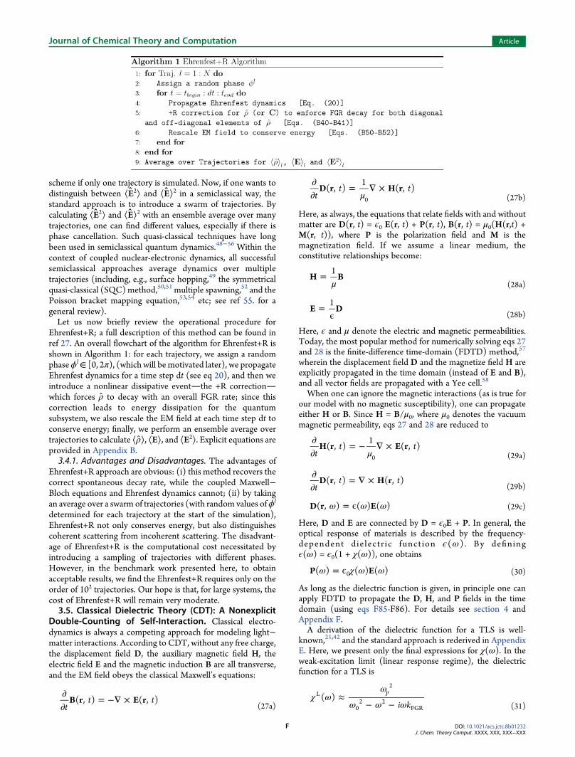
Ehrenfest+R; a full description of this method can be found inref 27. An overall flowchart of the algorithm for Ehrenfest+R isshown in Algorithm 1: for each trajectory, we assign a randomphaseϕl∈ [0, 2π), (which will be motivated later), we propagateEhrenfest dynamics for a time step dt (see eq 20), and then weintroduce a nonlinear dissipative eventthe +R correctionwhich forces ρ to decay with an overall FGR rate; since thiscorrection leads to energy dissipation for the quantumsubsystem, we also rescale the EM field at each time step dt toconserve energy; finally, we perform an ensemble average overtrajectories to calculate ⟨ρ⟩, ⟨E⟩, and ⟨E2⟩. Explicit equations areprovided in Appendix B.3.4.1. Advantages and Disadvantages. The advantages of

Ehrenfest+R approach are obvious: (i) this method recovers thecorrect spontaneous decay rate, while the coupled Maxwell−Bloch equations and Ehrenfest dynamics cannot; (ii) by takingan average over a swarm of trajectories (with random values ofϕl

determined for each trajectory at the start of the simulation),Ehrenfest+R not only conserves energy, but also distinguishescoherent scattering from incoherent scattering. The disadvant-age of Ehrenfest+R is the computational cost necessitated byintroducing a sampling of trajectories with different phases.However, in the benchmark work presented here, to obtainacceptable results, we find the Ehrenfest+R requires only on theorder of 102 trajectories. Our hope is that, for large systems, thecost of Ehrenfest+R will remain very moderate.3.5. Classical Dielectric Theory (CDT): A Nonexplicit

Double-Counting of Self-Interaction. Classical electro-dynamics is always a competing approach for modeling light−matter interactions. According to CDT, without any free charge,the displacement field D, the auxiliary magnetic field H, theelectric field E and the magnetic induction B are all transverse,and the EM field obeys the classical Maxwell’s equations:

tt tB r E r( , ) ( , )∇∂

∂= − ×

(27a)

tt tD r H r( , )

1( , )

0μ∇∂

∂= ×

(27b)

Here, as always, the equations that relate fields with and withoutmatter are D(r, t) = ϵ0 E(r, t) + P(r, t), B(r, t) = μ0(H(r,t) +M(r, t)), where P is the polarization field and M is themagnetization field. If we assume a linear medium, theconstitutive relationships become:

H B1μ

=(28a)

E D1=ϵ (28b)

Here, ϵ and μ denote the electric and magnetic permeabilities.Today, the most popular method for numerically solving eqs 27and 28 is the finite-difference time-domain (FDTD) method,57

wherein the displacement field D and the magnetize field H areexplicitly propagated in the time domain (instead of E and B),and all vector fields are propagated with a Yee cell.58

When one can ignore the magnetic interactions (as is true forour model with no magnetic susceptibility), one can propagateeither H or B. Since H = B/μ0, where μ0 denotes the vacuummagnetic permeability, eqs 27 and 28 are reduced to

tt tH r E r( , )

1( , )

0μ∇∂

∂= − ×

(29a)

tt tD r H r( , ) ( , )∇∂

∂= ×

(29b)

D r E( , ) ( ) ( )ω ω ω= ϵ (29c)

Here, D and E are connected by D = ϵ0E + P. In general, theoptical response of materials is described by the frequency-dependent dielectr ic funct ion ϵ(ω) . By definingϵ(ω) = ϵ0(1 + χ(ω)), one obtains

P E( ) ( ) ( )0ω χ ω ω= ϵ (30)

As long as the dielectric function is given, in principle one canapply FDTD to propagate the D, H, and P fields in the timedomain (using eqs F85-F86). For details see section 4 andAppendix F.A derivation of the dielectric function for a TLS is well-

known,21,42 and the standard approach is rederived in AppendixE. Here, we present only the final expressions for χ(ω). In theweak-excitation limit (linear response regime), the dielectricfunction for a TLS is

i k( ) pL

2

02 2

FGRχ ω

ω

ω ω ω≈

− − (31)

Journal of Chemical Theory and Computation Article

DOI: 10.1021/acs.jctc.8b01232J. Chem. Theory Comput. XXXX, XXX, XXX−XXX

F

which corresponds to a Lorentz medium. Here,

2 /p 122

0 0ω μ ω= ϵ ℏ . Beyond linear response, a nonlineardielectric function can be expressed to the lowest nonlinearorder in the series expansion of the incoming field (see AppendixE):

kEE

( ) ( ) 11

1 4( ) / s

NL L

02

FGR2

02

2χ ω χ ωω ω

≈ −+ −

| || |

Ä

Ç

ÅÅÅÅÅÅÅÅÅÅ

É

Ö

ÑÑÑÑÑÑÑÑÑÑ(32)

In eq 32, E0 is the amplitude of the incident wave defined in eq 3and we define |Es|

2 ≡ ℏ2 kFGR2/2 |μ12|

2. One interesting propertyof the series expansion leading to χNL is that the series convergesonly when |E0|/|Es| ≤ 1. Therefore, this expansion cannot beused to model very strong light−matter interactions.In Appendix E, we show that CDT (eq 29) with eq 31 for the

dielectric function double-counts self-interaction for a TLSbecause of a mismatch between the derivation of χ(ω) (whichassumes P = ϵ0 χEin) and the way the polarization is used withinCDT (P = ϵ0χE, eq 30). In other words, CDT suffers the sameproblem effectively as the coupled Maxwell−Bloch equation.

This double-counting becomes obvious if we evaluate theequation of motion for the optical polarization. See Table 1.

3.5.1. Advantages and Disadvantages. For CDT, onepropagates only Maxwell’s equations (i.e., no Schrodingerequation) in the time domain, and one can perform large-scalecalculations within a parallel architecture. The disadvantage ofCDT is that, by treating the matter side classically, one fails tocapture any quantum features of the light−matter interactions,unlike the case for semiclassical simulations. Furthermore, CDTdouble-counts self-interaction for a TLS in a similar manner tothe coupled Maxwell−Bloch equations.

3.6. Summary of Methods. After introducing the fivemethods above, we now summarize the main features of eachmethod in Table 1, highlighting (i) the ability to recover theFGR rate in spontaneous emission (SE), (ii) the effectiveequations of motion for the optical polarization (P), and (iii)whether or not energy is conserved. See Appendix C for allderivations.Note that in Table 1, we defineP rd Tr( ) Tr( )∫ μρ ρ= = ;

we also define 2 /p 122

0 0ω μ ω≡ ϵ ℏ as the plasmon frequency,

Table 1. Synopsis of the Main Features for the Five Different Approaches Chosen for Modeling Light−Matter Interactions

Approach Recover SE equation of motion for optical polarization energy conservation59

optical Bloch eqs 13 and 17 true P(t) + kFGRP(t) + ω02P(t) = ϵ0ωp

2W12(t) Ein(t) true (QOBE)/false (COBE)Maxwell−Bloch, eqs 12−16 false P(t) + kFGRP(t) + ω0

2P(t) = ϵ0ωp2W12(t)E(t) false

Ehrenfest, eqs 20 and 16 false (true only when ρ11→1) P(t) + ω02P(t) = ϵ0ωp

2 W12(t)E(t) trueEhrenfest+R, Appendix B true P(t) + 2γR(t)P(t) + [ω0

2 + γR(t) + γR2(t)]P(t) = ϵ0ωp

2W12(t)E(t) trueCDT-Lorentz, eqs 29−31 P(t) + kFGRP(t) + ω0

2P(t) = ϵ0ωp2E(t) false

Figure 1. Electronic dynamics of a TLS excited by an incident cw field: (upper) the excited state population (ρ22) versus time, (bottom) the imaginarypart of coherence Im ρ12 versus time. Four different conditions are plotted: (from left to right) weak on-resonant field (Ω/kFGR = 0.03, ω = ω0), weakoff-resonant field (Ω/kFGR = 0.03, (ω−ω0)/kFGR = 0.64), slightly stronger on-resonant field (Ω/kFGR= 0.3,ω =ω0) and slightly stronger off-resonantfield (Ω/kFGR= 0.3, (ω − ω0)/kFGR = 0.64). In each subplot, four methods are compared: (i) Ehrenfest dynamics (cyan solid), (ii) the Ehrenfest+Rapproach (red solid), (iii) the OBE (dashed-dotted green), and (iv) the coupledMaxwell−Bloch equations (dashed blue). Other parameters are listedin section 4. Note that for the weak coupling case, Ehrenfest, Ehrenfest+R, andOBE roughly agree. For the case of the stronger incident field, Ehrenfest+R predicts almost the same results as the OBE; Ehrenfest dynamics overestimate the electronic response at resonance because the method ignores ofvacuum fluctuations. The coupledMaxwell−Bloch equations underestimate the electronic dynamics in all situations because of the double-counting ofself-interaction.

Journal of Chemical Theory and Computation Article

DOI: 10.1021/acs.jctc.8b01232J. Chem. Theory Comput. XXXX, XXX, XXX−XXX

G

W12≡ ρ11− ρ22, Ein(t) and E(t) are short for Ein(0,t) and E(0,t).From the equations of motion of P for each method, we canclearly ascertain whether a method double-counts self-interaction or not. For example, in the coupled Maxwell−Bloch equations as well as CDT, both a dissipative term kFGRPand the total E-field appears, indicating a double-counting ofself-interaction.

4. NUMERICAL DETAILSOur parameters are chosen as follows (listed both in naturalunits c =ℏ= ϵ0 = 1 and [t] = 1× 10−17 s as well as in SI units): theenergy difference of TLS is ℏω0 = 0.25 (16.5 eV), the transientdipole moment is μ12 = 0.025√2 (11282 C·nm/mol), the widthof the TLS is σ = 0.50 (1.5 nm). We propagate Maxwell’sequations on a 1D grid with spatial spacing Δx = 0.10 (0.3 nm),time spacing Δt = 0.05 (5 × 10−4 fs), and our spatial domainranges from xmin = −4 × 104 (−12 μm) to xmax = 4 × 104 (12μm). The propagation time is tmax = 105 (1 ps). We calculate thesteady-state intensity of the EM field by averaging the EM fieldgenerated in the time range [tmax − t0, tmax], where t0 = 104 (100fs).For the CDT simulation, we use FDTDwith the standard Yee

cell.58 For a Lorentz medium (χL(ω)), we propagate eqs 29, 30,and C63 simultaneously as is standard.60 For the nonlinear

dielectric function χNL(ω) in eq 32, since the incident field ism o n o c h r o m a t i c , w e n e e d s i m p l y t o t r e a t

1k

EE

11 4( ) / s0

2FGR

20

2

2−ω ω+ −

| || |

ÄÇÅÅÅÅÅÅÅ

ÉÖÑÑÑÑÑÑÑ as a constant during the simulation

so that the equations of motion are similar to the linear case. Thestandard trick for simulating dynamics with a Lorentzsusceptibility is repeated in Appendix F.For all methods apart from CDT, all time derivatives for fields

and matter are propagated by a Runge−Kutta fourth-ordersolver61 and spatial gradients are evaluated on a real space gridwith a two-stencil. For the Ehrenfest+R approach, we averageover 48 trajectories unless stated otherwise.

5. RESULTS

In this section, we report the electronic dynamics and the steady-state optical signals arising when an incident cw field excites aTLS starting in the ground state.

5.1. Electronic Dynamics. Figure 1 shows the electronicdynamics of a TLS as a function of time for all methods (exceptCDT for which there are no explicit TLS dynamics). Amongthese methods, the OBE (green dashed-dotted line) can beregarded as a “standard” method for all conditions. Our resultsare as follows.

Figure 2. Steady-state intensities (integrated over all frequencies) for the scattered E-field for a TLS as a function of frequency of the incident cw field:(left) weak incident field (Ω/kFGR = 0.03) and (right) slightly stronger incident field (Ω/kFGR = 0.3). Six methods are compared (from top to bottom):(i) Ehrenfest dynamics (cyan), (ii) the Ehrenfest+R approach (red for coherent scattering and gray for total scattering intensity), (iii) the OBE(green), (iv) the coupled Maxwell−Bloch equations (blue), (v) CDT with a Lorentz medium (black, χL(ω) given in eq 31), and (vi) CDT with anonlinear medium (purple, χNL(ω) given in eq 32). Simulation data (dots) are fitted to a Lorentzian function defined in eq 33, and the fittedparameters are also labeled (integral area and fwhm of Lorentzian). Simulation parameters are listed in section 4. Note that in the linear responseregime (left), Ehrenfest and Ehrenfest+R agree with the OBE, whileMaxwell−Bloch and CDT predict different results because of the double-countingof self-interaction. Beyond linear response (right), Ehrenfest dynamics overestimate the intensity and underestimate the fwhm because of the absenceof vacuum fluctuations; Ehrenfest+R and the OBE predict the correct trends: less intense and broader peaks, which are known as saturation effects; forMaxwell−Bloch or CDT, these tendencies are not obvious. Finally, when including only the third-order nonlinear term, the performance of CDT is notenhanced, as the method still does not capture the broadening correctly.

Journal of Chemical Theory and Computation Article

DOI: 10.1021/acs.jctc.8b01232J. Chem. Theory Comput. XXXX, XXX, XXX−XXX

H

1. For a weak on-resonant cw field (Ω/kFGR = 0.03,ω =ω0),both Ehrenfest (cyan solid) and Ehrenfest+R (dashedred) quantitatively agree with the OBE for the evolutionof the excited state population ρ22 (Figure 1a) and theimaginary part of Imρ12 (Figure 1e). Ehrenfest andEhrenfest+R agree in the limit of weak excitation (wherethe +R correction [proportional to ρ22] for Ehrenfest+R isnegligible) and both methods agree with the correct OBE.That being said, the coupled Maxwell−Bloch equations(blue solid) predict different results: both ρ22 and Imρ12are drastically suppressed (see Figures 1a,e) because ofthe double-counting of self-interaction.

2. For a weak off-resonant cw field (Ω/kFGR = 0.03,(ω−ω0)/kFGR = 0.64), not surprisingly, the dynamicsfor ρ22 and Imρ12 are suppressed (Figures 1b,d,respectively) compared with the resonant case. Interest-ingly, both Ehrenfest and Ehrenfest+R predict a slightlyhigher response of ρ22 compared with the OBE. Thisslight difference originates from two factors. (i) Theeffective Ehrenfest dissipative term EScatt

ρ[ ] approachesSE ρ[ ] near the ground state only in a coarse-grained

sense. (ii) More importantly, the off-diagonal Ehrenfestterm EScatt

ρ[ ] is purely imaginary, which leads to slightlyless dephasing compared with the SE ρ[ ] term from theOBE, which has a real part, e.g., kFGRρ12/2. Thus, the OBEand Ehrenfest do not yield the exact same dynamics eventhough the absolute values of the off-diagonal compo-nents of both EScatt

ρ[ ] and SE ρ[ ] are identical. SeeAppendix A for a detailed discussion. Again, Maxwell−Bloch disagrees with all of the other methods because ofdouble-counting.

3. When the cw field is amplified to slightly beyond the weakcoupling limit (Ω/kFGR = 0.3), the new feature that arisesis that Ehrenfest now over-responds both for ρ22 and ρ12compared with the OBE; at the same time, Ehrenfest+Rstill nearly agrees with the OBE, just as in the weakcoupling case. Obviously, the inclusion of vacuumfluctuations becomes more and more important as theamplitude of the incident field and the excited statepopulation increases. For strong fields, Ehrenfest+Rbecomes an important correction to Ehrenfest dynamics.

5.2. Steady-State Optical Signals. In Figure 2, we plot thesteady-state intensity of the scattered field (|Escatt|

2/|E0|2) as a

function of incident cw wave frequency ((ω − ω0)/kFGR) whenthe light−matter coupling (Ω/kFGR) is weak (Ω/kFGR = 0.03,left) and relatively strong (Ω/kFGR = 0.3, right). Note that weplot the overall scattered field intensity, integrated over allfrequencies. While the dots in Figure 2 represent the simulationdata with specific incident frequenciesω, we also fit these data toa Lorentzian in order to better capture the line width and themagnitude of the optical signal; the Lorentzian is defined as

( )f

A( )

( )

12

02 1

2

2ωπ ω ω

=Γ

− + Γ (33)

where A denotes the total integrated area of f(ω) and Γ denotesthe full width at half-maximum (fwhm) of f(ω).For the weak coupling (Ω/kFGR = 0.03; see Figure 2a), just as

for electronic dynamics (see Figure 1), Ehrenfest (cyan) andEhrenfest+R (red) agree with the OBE (green) while bothMaxwell−Bloch (blue) and CDT (black for linear χ and purple

for nonlinear χ) predict different results. When the excitation isweak, Ehrenfest, Ehrenfest+R, and theOBE correctly predict theFGR rate for the electronic relaxation, which now becomes thefwhm for the line shape. Due to the double-counting of self-interaction, however, the coupled Maxwell−Bloch equationsand CDT predict twice the correct fwhm; see the detaileddiscussion in Appendix C. Lastly, we note that, if one wants touse CDT to predict the correct fwhm for a TLS, one can reducethe width of the dielectric function in half (i.e., reduce kFGR tokFGR/2 in eq 31) and efficiently avoid double-counting.However, we emphasize that generalizing this result to largerquantum subsystems (e.g., beyond a TLS) is either tedious orimpossible. For this reason, in this paper, we have used thestandard susceptibility for a TLS, i.e., eqs 31 and 32, as found inrefs 21 and 42.Now let us move to a slightly stronger cw field (Ω/kFGR = 0.3).

See Figure 2b. We do not choose a very large field because thenonlinear FDTD simulation will become unstable whenΩ/kFGR→ 1 due to the convergence issue of χNL(ω) ; see eq E83. Foreven a moderately strong field (Ω/kFGR = 0.3), the OBE predictsa saturation effect, for which the intensity of the scattered field issuppressed and the fwhm is broadened. Similar tendencies canalso be found in Ehrenfest+R.Interestingly, for the coupled Maxwell−Bloch equations, a

saturation effect is not obvious because of the double-countingof self-interaction. Furthermore, because Ehrenfest does notinclude vacuum fluctuations, this method predicts the exactlyincorrect trend: the fwhm decreases for large incident fields.Finally, regarding CDT, it is not surprising at all that the linearLorentz medium results do not change when the incident fieldstrength is increased. More interestingly, even if we include thelowest order of nonlinearity, CDT predicts the incorrect trendfor the absorption fwhm (just like Ehrenfest). Apparently,including only the lowest order of nonlinearity is not enough foran accurate description of optical signals outside of linearresponse.Finally, before concluding, we note that Ehrenfest+R also

makes a prediction of the total scattering intensity (⟨|E|2⟩). Assuch, Ehrenfest+R differs from all the other methods presentedin Figure 2, which predict only the intensity of coherentscattering. The only other method which can make prediction ofcoherent versus incoherent EM dynamics is the quantum OBE(see section 3.2), which is considered the gold standard formodeling a quantum field of photons interacting with a TLS.Although we do not plot the quantum OBE results in Figure 2,we will compare Ehrenfest+R with the quantum OBE below inthe Discussion.

6. DISCUSSION

The above results demonstrate that the Ehrenfest+R approachmay be an advantageous method to model light−matterinteractions: this method not only predicts similar electronicdynamics and the same coherent scattered field as the classicalOBE, but also directly models the total scattered field byenforcing energy conservation so that one can predict ⟨E2⟩ and⟨E⟩2 independently. Thus, in the future, we believe we will beable to use the Ehrenfest+R approach to correctly model light−matter interactions for many emitters (without the requirementof excluding self-interaction, as needed for the coupledMaxwell−Bloch equations). Because so many collective opticalphenomena have been recognizedfor example, resonantenergy transfer,23,62,63 superradiance,64−66 and quantum

Journal of Chemical Theory and Computation Article

DOI: 10.1021/acs.jctc.8b01232J. Chem. Theory Comput. XXXX, XXX, XXX−XXX

I

beats67the Ehrenfest+R approach is a very tempting tool togeneralize and apply.That being said, it remains to demonstrate that the Ehrenfest

+R approach predicts the correct total scattered field ascompared with the quantum OBE. To that end, in Figure 3

we plot the ratio between the coherent and total scattered fields(Icoh/Itot) for a wide range of field intensities (Ω/kFGR) for thecase that the TLS is excited on resonance by an incident cw field(ω = ω0). From Figure 3, results for Ehrenfest+R (open circle)quantitatively match the theoretical prediction calculated byMollow38 (dashed line):

II

k

k

( )

( )coh

tot

02 1

4 FGR2

12

20

2 14 FGR

2

ω ω

ω ω=

− +

Ω + − + (34)

The quantitative agreement between Ehrenfest+R and theanalytical calculation based on the quantumOBE in Figure 3 canbe understood as follows. From the procedure of Ehrenfest+R(see section 3.4), we are guaranteed both that the excited statewill relax with the FGR rate and that energy will be conserved.On the one hand, because of the correct electronic relaxation,Ehrenfest+R must predict nearly the same electronic dynamicsas the OBE, so that the coherent scattered field predicted byEhrenfest should be accurate. On the other hand, becauseenergy is conserved at each time step, the total intensity of thescattered field has to be correct. By combination of these twosides, it is not surprising that Ehrenfest+R predicts Icoh/Itotquantitatively. However, for very strong incident fields, beyondthe correct prediction of intensities, one can wonder: willEhrenfest+R also quantitatively capture the f requency dependenceof the scattered fields (which is not required in an algorithm ofEhrenfest+R)? For example, can Ehrenfest+R recover theMollow triplet38 correctly? Preliminary results are encour-aging.68

7. CONCLUSIONIn this paper, we have benchmarked the performance of fivemethods (the coupled Maxwell−Bloch equations, the classicalOBE, Ehrenfest, Ehrenfest+R, and CDT) for modeling light−matter interactions. When studying a TLS excited by an incident

cw field, we find the following: (i) Because Ehrenfest dynamicsinclude only self-interaction for electronic relaxation, thismethod fails to correctly describe the electronic dynamics andoptical signals beyond the linear response regime. (ii) Thecoupled Maxwell−Bloch equations and CDT fail to predict thecorrect optical signals even in the linear response regime,because both methods effectively double-count self-interaction:the self-interaction is accounted for through the spontaneousemission with both the scattered field and an explicit dissipativeterm; see eq 12. As a consequence, these methods predictspectra with twice the correct fwhm in Figure 2. (iii) Becauseboth the classical OBE and the Ehrenfest+R approach carefullycount self-interaction only once (but in different ways), thesetwo methods describe both the electronic dynamics and theoptical signals correctly in both the linear response regime andslightly beyond linear response. Moreover, because Ehrenfest+Rpreserves the self-interaction due to the scattered field and alsoenforces electronic relaxation due to vacuum fluctuations, thisapproach should be applicable for modeling light−matterinteractions for a network of molecules, whereas for the OBE,one would need to carefully exclude the self-interaction due tothe scattered field. Finally, by conserving energy, Ehrenfest+Rcan correctly distinguish between coherent and incoherentscattering over a wide range of light−matter couplings and allresults are in agreement with the quantum OBE.The role of the total scattered field is essential for many

collective phenomena, including, for example, resonant energytransfer and superradiance, and our laboratory is very excited tolearn what new physics can be predicted with a powerful, newsemiclassical approach to electrodynamics.

■ APPENDIX A: ELECTRONIC RELAXATION WITHINEHRENFEST DYNAMICS

One significant difference between Ehrenfest dynamics and theother methods studied in this paper is that the equation ofmotion for Ehrenfest dynamics has no explicit dissipative term;see eq 20a. One may ask, do Ehrenfest dynamics still recoverelectronic relaxation? Here, for completeness, we summarize themain points in ref 27.To understand electronic relaxation for Ehrenfest dynamics,

we can split the total E-field into the incident field plus thescattered field: E(r, t) = Ein(r,t) + Escatt(r, t). While the incidentfield obeys Ein(r, t) = Ein(r− ct, 0), we must explicitly propagateEscatt(r, t) and solve Maxwell’s equations. In 1D, if we initializethe TLS such that Imρ12(0) = 0 at time zero, the solution forEscatt is

22

x tc

t t x xE ( , ) d Im ( ) d ( )t

x c t t

x c t t

scatt0

0 0 12 ( )

( )∫ ∫ ξ

ωρ=

ϵ′ ′

′

′ ′ ′− −

+ −

(A35)

where ξ(x) = μ12 δ(x) if we assume a point-dipole, and ρ12 is thet ime der i va t i ve o f ρ 1 2 , so tha t μ ·E s c a t t (0 , t) =

∫ dx ξ(x)·Escatt(x, t) σx = ℏkFGR Imρ12σx, where ( )0 11 0xσ = .

By substituting eq A35 into eq 20a, one finally obtains

tdd E

E E

s

s in scatt

ρ ρ ρ

ρ ρ ρ

= [ ] + [ ]

= [ ] + [ ] + [ ] (A36)

where s ρ[ ] and Einρ[ ] are defined in eq 23 and

Figure 3. Ratio between the steady-state intensities of coherent andtotal scattered fields (Icoh/Itot) as a function of light−matter coupling(Ω/kFGR) when a TLS is excited by an incident cw field at resonance (ω= ω0). Ehrenfest+R result (open circle) is compared with thetheoretical prediction (dashed line) in eq 34. A total of 480 trajectoriesare averaged for Ehrenfest+R. All other parameters are the same as inFigure 2.

Journal of Chemical Theory and Computation Article

DOI: 10.1021/acs.jctc.8b01232J. Chem. Theory Comput. XXXX, XXX, XXX−XXX

J

i t

ki

i

E 0( , ),

2 Im Im ( )

Im ( ) 2 Im

E scatt

FGR12

212 11 22

21 11 22 122

scattμρ ρ

ρ ρ ρ ρ

ρ ρ ρ ρ

[ ] =ℏ

[ · ]

=[ ] − −

− − − [ ]

i

k

jjjjjjjj

y

{

zzzzzzzz(A37)

Equation A37 defines kEh and γEh in eq 24, which clearly showsthat the scattered field contributes to the electronic relaxation ifImρ12≠ 0. Furthermore, though not proven here, eq A37 is validin 3D (as well as 1D).27 We will now analyze eq A37 in the weakcoupling limit.Population Relaxation RateIn the weak coupling limit, ω0 ≫ kFGR, and we can define a timescale (τ) 1/ω0 ≪ τ ≪ 1/kFGR. With this time scale, one canassume ρ12 ≈ |ρ12|e

iω0t so that [Imρ12]2 ≈ |ρ12|

2 sin2(ω0t). Wemay then define an instantaneous decay rate kEh(t) for ρ22,satisfying ρ22 = −kEh(t) ρ22, where

k t k t( ) 2 sin ( )Eh FGR12

2

22

20

ρρ

ω=| |

[ ](A38)

We call eq A38 the Ehrenfest decay rate. If we average this rateover all relevant τ, we find tsin ( )2

012

ω = , and one obtains eq 25.

For Ehrenfest dynamics, because no non-Hamiltonian termappears in the Liouville equation, purity is strictly conserved, sothat |ρ12|

2 = ρ11ρ22, and eq 25 reduces to eq 1.Off-Diagonal (Dipole) Dephasing RateWhen comparing the Ehrenfest effective dissipative term( Escatt ρ[ ] in eq A37) against the OBE ( SE ρ[ ] in eq 13), wefind one interesting disagreement: for Ehrenfest dynamics, theoff-diagonal dissipation is purely imaginary, but for the OBE,there is a real component. When averaged over a time τ, theabsolute values of these off-diagonal terms remain the same.However, as shown in Figs. 1b,d, this difference causes theelectronic dynamics for Ehrenfest dynamics to differ slightly ascompared with the OBE when an off-resonant cw field excitesthe TLS. This difference can be explained as follows. On the onehand, for the classical OBE, if we consider only the effect of the

dipole-dephasing for ρ12, i.e., tdd 12 12ρ γρ= − , the off-diagonal

density matrix element clearly satisfies ρ12(t) = e−γtρ12(0).On the other hand, for Ehrenfest dynamics, even though we

still findt

dd 12 12ρ γρ= − , γ is now purely imaginary (see eq A37).

Hence, it is natural to consider the absolute value of ρ12, which

satisfiest

dd 12ρ| | = −γEh(t) |ρ12|,

t k t( ) ( ) sin ( )Eh FGR 11 222

0γ ρ ρ ω= − (A39)

In a coarse-grained picture, γEh(t) reduces to eq 26. When ρ11→1, γEh agrees with the OBE (γBloch = kFGR/2) and Ehrenfest+R isnot needed. Thus, the major difference between Ehrenfest+Rand the OBE is just the phase of dipole dephasing rate γ, whichcan lead to a slight difference in ρ12 at later times.

■ APPENDIX B: DETAILS OF THE EHRENFEST+RAPPROACH

B.1. +R Correction for the Electronic DynamicsAccording to Ehrenfest dynamics, including self-interactionleads to incorporating some fraction of the true FGR rate ofelectronic relaxation ( Escatt

ρ[ ] in eq 24; see also eqs 25 and 26).

In order to correctly recover the full FGR decay rate, Ehrenfestdynamics include an additional dissipative (“+R”) term ( R ρ[ ])on top of the normal Liouville equation in eq 20a. At every timestep, we write

t dt t t t t t( ) ( d ) ( d ) dEh R Eh R Ehρ ρ ρ + = + + [ + ]+(B40)

Here, ρEh refers to the electronic density operator that ispropagated with Ehrenfest dynamics for one time step; R ρ[ ] isdefined as

k t t

t k t

( ) ( )

( ) ( )R

R 22 R 12

R 21 R 22

ρρ γ ρ

γ ρ ρ[ ] =

−

− −

i

k

jjjjjjjy

{

zzzzzzz (B41)

where we define kR and γR to be the +R population relaxationand dipole dephasing rates, respectively:

k t k( ) 2 1 Im eiR FGR

122

22

12

12

2lρ

ρρρ

≡ −| |

| |ϕ

Ä

Ç

ÅÅÅÅÅÅÅÅÅÅÅ

É

Ö

ÑÑÑÑÑÑÑÑÑÑÑ

Ä

Ç

ÅÅÅÅÅÅÅÅÅÅ

É

Ö

ÑÑÑÑÑÑÑÑÑÑ (B42a)

tk

( )2

(1 )RFGR

11 22γ ρ ρ≡ − +(B42b)

According to eq B42a, each trajectory l experiences its own kR(t)with an arbitrary phase ϕl ∈ [0, 2π). Note that this phase doesnot change during the simulation. From our point of view,introducing this stochastic element on top of Ehrenfestdynamics is entirely reasonable; and similar approaches havealready been proposed in the context of nuclear-electronicdynamics.69−72

In a coarse-grained picture, averaging over the random phase

ϕl, one finds Im ei2

12

l12

12=ρ

ρϕ

| |

ÄÇÅÅÅÅÅÅÅ

ÉÖÑÑÑÑÑÑÑ , so that

k t k( ) 1R FGR12

2

22

ρρ

= −| |i

kjjjjjj

y

{zzzzzz (B43)

Thus, the total emission (including the self-interaction of thescattered field in Ehrenfest dynamics ( Escatt

ρ[ ] in eq 24) plusthe +R quantum vacuum fluctuations pathway ( R ρ[ ] in eqB41)) is identical to the total dissipation found in the OBE( SE ρ[ ] in eq 13):

k t k t k( ) ( )Eh R FGR+ = (B44a)

t tk

( ) ( )2Eh R

FGRγ γ+ =(B44b)

+R Correction in the Wave Function PictureOne appealing quality of Ehrenfest dynamics is that the purity ofthe electronic subsystem does not change within a singletrajectory, and one can propagate Ehrenfest dynamics with adensity operator ρ or a wave function C. The Ehrenfest+Rapproach is consistent with this structure, and can beimplemented in the wave function picture as well:

t t k t tC C( d ) e ( d )iEh R 1 2 R Eh

R+ = [ ] +γ+

Φ[ ]← (B45)

Here, CEh is the quantum amplitude after one time steppropagated according to Ehrenfest dynamics, and CEh+R is thecorresponding quantum amplitude after the +R event. Thequantum transition operator k1 2 R

[ ]← in eq B45 is responsible

Journal of Chemical Theory and Computation Article

DOI: 10.1021/acs.jctc.8b01232J. Chem. Theory Comput. XXXX, XXX, XXX−XXX

K

for enforcing additional population relaxation, and changes C toC′:

kcc

c

c1 2 R1

2

1

2

[ ] =′

′←ikjjjj

y{zzzz

i

kjjjjjj

y

{zzzzzz (B46)

For a TLS, the relationship between C′ and C is

ccc

c k t c t( ) d11

11

2R 2

2′ =| |

| | + | |(B47a)

ccc

c k t c t( ) d22

22

2R 2

2′ =| |

| | − | |(B47b)

where kR is defined in eq B42a. When c1 = 0 (and the electronicsubsystem is in the excited state), kR = kFGR, and

cc

1

1| |and c

c2

2| |are

not well-defined. For a practical implementation, when c1 = 0, weforce 1c

c1

1=

| | and we fix ecc

i2

2= θ

| | , where θ ∈[0, 2π) is a randomnumber. Note that θ and ϕl have no correlation.In eq B45, after invoking the quantum transition operator

k1 2 R [ ]← , we next multiply by a stochastic random phase

operator eiΦ[γR] to enforce the additional dipole dephasing:

te

e 00 1

, if RN d

1, otherwise

i

i

RR

0

γ=

<

γΦ[ ]

Φl

moooooo

noooooo

ikjjjj

y{zzzz

(B48)

where 1 is the identity operator. Φ0 and RN are independentrandom numbers with range Φ0 ∈ [0, 2π) and RN ∈ [0, 1).During the time interval dt, eq B48 efficiently reduces theensemble average coherence ⟨c1c2*⟩ by an amount γR dt⟨c1c2*⟩.Note that, for Figures 1−3, we have confirmed numerically

that propagating the +R correction in the wave function picture(eqs B45−B48) yields the same results compared with thedensity matrix picture (eqs B40−B42). However, for strongerincoming fields, the two methods will not always agree. Forinstance, the wave function picture that uses stochasticdephasing (eq B48) can sucessfully predict a Mollow triplet,while the density matrix picture fails to do so; see ref 68 for moredetails. Hence, we recommend always implementing Ehrenfest+R with the wave function picture.B.2. Rescaling the EM FieldAfter enforcing the +R correction for the electronic subsystem,in order to conserve energy, one needs to rescale the classicalEM field at each time step dt by giving energyURto the EM field:

tU k t

dd

( )R 0 R 22ω ρ= ℏ(B49)

In practice, we rescale the EM field after every time step dt by

E E El l lEh R Eh Rα δ= ++ (B50a)

B B Bl l lEh R Eh Rβ δ= ++ (B50b)

where EEhl denotes the E-field for trajectory l with no field

rescaling and EEh+Rl denotes the E-field after field rescaling; the

rescaling functions δER and δBR are chosen according topolarization density and these fields should not self-interferewith the TLS or otherwise influence the propagation of ρ(because the addtion of R ρ[ ] already leads to the correctspontaneous decay rate). In 1D, for the polarization profiledefined in eq 7, these rescaling functions are defined as

x xE e( )2

e xzR

125

2 /22 2δ

μπ σ

= − σ−

(B51a)

x xB e( )3 2

e xyR

125

3 /22 2δ

μπ σ

= σ−

(B51b)

Mo r e g e n e r a l l y , i n 3D , ERδ ∇= × × a n dBRδ ∇= × .21,73 The parameters αl and βl are defined to

conserve the total energy:

c Uv

tE

sgn(Im e )d

dl i12

R

0 R2

l

∫α ρ

δ= [ ]

Λ

ϵ | |ϕ

(B52a)

ec U

vt

Bsgn(Im )

ddl i

120 R

R2

l

∫β ρ

μ

δ= [ ]

Λ

| |ϕ

(B52b)

Here, UR is short for Ut

dd R , and URis defined in eq B49; Λ is the

self-interference length, which is defined as

E

r E

B

r B

2 (0)

d

2 (0)

d

2R

2

R2

2R

2

R2∫ ∫

π δδ

π δδ

Λ =| |

| |+

| || | (B53)

δER and δBR are the Fourier components of the rescaling fieldsδER and δBR:

E r k E k( ) d ( )eik rR R∫δ δ= ·

(B54a)

B r k B k( ) d ( )eik rR R∫δ δ= ·

(B54b)

For the po l a r i z a t ion profi l e in eq 7 , we find

2.36343

σ σΛ = =π .

■ APPENDIX C: OPTICAL POLARIZATION FOR EACHMETHOD

C.1. The Optical Bloch EquationFor the OBE, one calculates the effective optical polarization,P(t), according to the mean-field approximation:

t tP( ) Tr( ( ) )μρ= (C55)

Here, one needs to be careful about notation. P denotes the totaloptical polarization, which is the integral over the polarizationdensity operator, r( ) in eq 6: P r rd Tr( ( ))∫ ρ= .By taking the second-order time derivative of eq C55, using

P = 2 Re ρ12μ12ez, calculating Ret

dd 12ρ and Im

tdd 12ρ and further

applying eqs 9 and 17, the equation of motion for P(t) can beexpressed as

t k t t W t tP P P E( ) ( ) ( ) ( ) ( )pFGR 02

02

12 inω ω + + = ϵ (C56)

Here, we define 2 /p 122

0 0ω μ ω≡ ϵ ℏ to be the plasmonfrequency, W12 ≡ ρ11 − ρ22, Ein(t) is short for Ein(0, t).Equation C56 is an anharmonic oscillator picture for optical

polarization.21 Given an initial condition for P, according theclassical OBE, one evolves eq C56 coupled with Maxwell’sequations in eq 15 to obtain the optical signals for a TLS.C.2. The Coupled Maxwell−Bloch EquationsFollowing the procedure for the OBE, one obtains a very similarequation of motion for optical polarization P in the case of thecoupled Maxwell−Bloch equations:

Journal of Chemical Theory and Computation Article

DOI: 10.1021/acs.jctc.8b01232J. Chem. Theory Comput. XXXX, XXX, XXX−XXX

L

t k t t W t tP P P E( ) ( ) ( ) ( ) ( )pFGR 02

02

12ω ω + + = ϵ (C57)

Here,ωp andW12 are defined the same as in eq C56. Comparingeq C57 to eq C56, because E = Ein + Escatt, we see that the opticalpolarization can be significantly different if the scattered field isnot negligible.C.3. Ehrenfest DynamicsFor Ehrenfest dynamics, from eq 20, the equation of motion forthe optical polarization is easy to derive:

t t W t tP P E( ) ( ) ( ) ( )p02

02

12ω ω + = ϵ (C58)

Compared to the other equations of motion for P in eqs C56 andC57, the major difference is that eq C58 has no explicitrelaxation term (kFGRP). However, the lack of such a relaxationterm does not imply that the anharmonic oscillator will not bedamped to zero at long times. In fact, since P = Tr(ρμ), and ρ isrelaxed by the scattered field Escatt (see the discussion in section3.3.1), P will eventually be damped to zero as long as the TLS isnot initiated exactly in the excited state. More explicitly, if weseparate the electric field as E = Escatt + Ein, and use the fact that

kE Im ktscatt FGR 12

d Re

dFGR

0

12μ ρ· = ℏ = −ω

ρℏ [ ], where we denote μ =

μ12ez, eq C58 can be rewritten as

t W t k t W t tP P P E( ) ( ) ( ) ( ) ( )p12 FGR 02

02

12 inω ω + + = ϵ(C59)

Here, the effective relaxation term W12(t) kFGRP causes apopulation-dependent damping for P.C.4. The Ehrenfest+R approachFor Ehrenfest+R, the equation of motion for optical polarizationreads

t t t t t t

W t t

P P P

E

( ) 2 ( ) ( ) ( ) ( ) ( )

( ) ( )p

R 02

R R2

02

12

γ ω γ γ

ω

+ + [ + + ]

= ϵ (C60)

where γR is defined in eq B42. To derive eq C60, we simply take

advantage of H ,t

idd sc Rρ ρ ρ = − [ ] − [ ]

ℏ, where Hsc and R ρ[ ]

are defined in eqs 19 and B41, and we find

dt

tRe

dIm ( ) Re12

0 12 R 12

ρω ρ γ ρ

[ ]= − −

(C61a)

tW tE

d Im

dRe ( ) Im12

0 12 12 R 12μρ

ω ρ γ ρ[ ]

= − · −

(C61b)

By taking the time derivative of eq C61a and applying eq C61b,we obtain

tW t

t

tt

t

Ed Re

dRe ( ) Im

d ( )

dRe ( )

d Re

d

212

2 0 0 12 12 R 12

R12 R

12

μρ

ω ω ρ γ ρ

γρ γ

ρ

[ ]= − [ − · − ]

− −[ ]

(C62)

Note that, if we set γR(t) = 0, we recover eq C58. Nevertheless, ifγR(t) ≠ 0, note also that eq C62 still contains Imρ12. Toeliminate this term, we can rewrite eq C61a as

tIm ( ) Ret12

1R 12

d Re

d0

12ρ γ ρ= −ω

ρ[ ]ÄÇÅÅÅÅÅÅ

ÉÖÑÑÑÑÑÑ. By substituting this iden-

tity into eq C62, we finally derive eq C60.In eq C60, by introducing the relaxation term 2γR(t) P(t)

where γR(t) depends on the electronic state, one recovers the

FGR rate correctly as compared with Ehrenfest dynamics. Oneinteresting feature of eq C60 [as compared with eqs C56−C58]is that the intrinsic frequency is no longer ω0 but rather

t t( ) ( )02

R R2ω γ γ+ + . This frequency renormalization will be

studied in a future publication.C.5. CDTThe susceptibility χ(ω), which is derived in Appendix E for aTLS, plays a significant role in classical electrodynamics. If wetake the Fourier transform of the definition of χ(ω) in eqs30−31, we find that the equation of motion for the opticalpolarization reads

t k t t tP P P E( ) ( ) ( ) ( )pFGR 02

02ω ω + + = ϵ (C63)

eq C63 is very similar to eq C57 in the weak-excitation limit(W12 → 1), indicating that a standard CDT treatment alsodouble-counts self-interaction, just as do the coupled Maxwell−Bloch equations. This double-counting originates from theinconsistency between the derivation of χ(ω)42 (where weassume P(ω) = ϵ0 χ(ω) Ein(ω)), and the numericalimplementation of CDT (where people frequently take P(ω)= ϵ0 χ(ω) E(ω) for a practical simulation); see Appendix E.

■ APPENDIX D: ENERGY CONSERVATION FOR EACHMETHOD

We define the energy of the quantum subsystem as

U t t H( ) Tr( ( ) )ss ρ= (D64)

For a classical EM field, the energy is defined as

U t t tr E r B r( )12

d ( , )1

( , )EM 02

0

2∫ μ= ϵ | | + | |

i

kjjjjj

y

{zzzzz

(D65)

For semiclassical approaches, the total energy is expressed asUtot= Us + UEM.D.1. The Optical Bloch EquationFor the OBE, similar to Ehrenfest dynamics (see eq 22), we canexpress eq 17 as

tdd s E SEin

ρ ρ ρ ρ = [ ] + [ ] + [ ](D66)

where s ρ[ ] and Einρ[ ] are defined in eq 23 and SE ρ[ ] is

defined in eq 13. If eq D66 is substituted into eq D64, the energyloss rate for the TLS reads

tU H H

dd

Tr( ) Tr( )s ss E SEinρ ρ= [ ] + [ ]

(D67)

By taking the time derivative of eq D65, and applying Maxwell’sequations as defined in eq 20, the energy gain rate of the EM fieldis

tU s E B r E J

dd

d dEM ∮ ∫= × − ·Σ (D68)

Here,Σ denotes the sphere in real space over which we integrate.If we integrate over a large sphere, the first term on the RHS ineq D68 vanishes.However, because one cannot find an exact cancellation

between eqs D67 and D68, the total energy of the classical OBEis not conserved. That being said, if the EM dynamics arepropagated with the quantum EM field instead of classical EMfield, the quantum OBE should conserve energy, provided weuse the full quantum energy of the EM field:

Journal of Chemical Theory and Computation Article

DOI: 10.1021/acs.jctc.8b01232J. Chem. Theory Comput. XXXX, XXX, XXX−XXX

M

U t t tr E r B r( )12

d ( , )1

( , )EM 02

0

2∫ μ′ = ϵ ⟨ ⟩ + ⟨ ⟩

i

kjjjjj

y

{zzzzz

(D69)

Formore details about the quantumOBE and eqD69, see ref 43.D.2. The Coupled Maxwell−Bloch EquationsJust as for the classical OBE, according to the coupledMaxwell−Bloch eqs (eq 12), the energy loss rate for a TLS reads

tU H H

dd

Tr( ) Tr( )s ss E SEρ ρ= [ ] + [ ] (D70)

The energy gain for the EM field is the same as eq D68. Aftersome straightforward algebra, we find the total energy obeys

tU H tE 0

dd

Tr( ( ( , ))) 0stot SE μρ= [ ] − · ≠(D71)

In most situations, the magnitude of the coupling |μ·E(0, t)| ismuch less than ℏω0. Under such conditions, we can furthersimplify eq D71 to read

tU H k

dd

Tr( ) 0stot SE 0 FGR 22ρ ω ρ≈ [ ] = −ℏ <(D72)

eqs D71-D72 show that energy is not conserved for the coupledMaxwell−Bloch equations and the total energy is continuouslydecreasing with a speed of ℏω0kFGRρ22. This failure cannot becorrected by propagating quantum fields and using QED (as ineq D69). The fundamental problem is not a quantum-classicalmismatch but rather a double-counting of self-interaction.D.3. Ehrenfest DynamicsAs discussed above, for Ehrenfest dynamics, the energy loss ratefor a TLS is expressed as

tU H

dd

Tr( )ss E ρ= [ ] (D73)

where E ρ[ ] is defined as

itE 0( , ),E μρ ρ[ ] =

ℏ[ · ]

(D74)

Since the energy gain rate for the EM field is defined just as in eqD68, the time derivative of the total energy can be expressed as

tU H

H t

r E J

E 0

dd

Tr( ) d

Tr( ) ( , ) Tr( )

0

s

s

tot E

E s

∫μ

ρ

ρ ρ

= [ ] − ·

= [ ] − · [ ]

= (D75)

w h e r e w e a p p l y J rTr( ) Tr( ) ( )μ δρ ρ= = a n d

s Eρ ρ ρ = [ ] + [ ] for Ehrenfest dynamics. Here, s ρ[ ] isdefined in eq 23. Thus, energy is conserved for Ehrenfestdynamics if we integrate over all space (where E and B fieldsvanish at the boundary).D.4. The Ehrenfest+R ApproachEhrenfest+R is designed to yield energy conservation providedone averages over trajectories; the total average Ehrenfest+Renergy reads

U H r E

B

Tr( )12

d

1

s l

l

tot 0 Eh R2

0Eh R

2

∫ρ

μ

= + ϵ ⟨| | ⟩

+ ⟨| | ⟩

+

+

i

kjjjjj

y

{zzzzz

(D76)

where ⟨···⟩l denotes an ensemble average over trajectoriesindexed by l ∈{1, 2,···, N}. Here, N is the total number oftrajectories. Because Ehrenfest dynamics alone conserve energy,we need to show only that the energy loss for the quantumsubsystem due to the + R correction balances the energy gain forthe EM field due to the rescaling of fields at every time step dt.This can be proved by induction: (i) suppose that, at time t, thetotal energy is conserved; (ii) at t + dt, dUR(t + dt) =ℏω0 kR(t + dt)ρ22 dt needs to be dissipated to the classical EMfield; see eq B49. After the rescaling of EM field by eqsB50−B52, the non-zero energy increment for the EM field hasthree components: (1) the squared norm of the added +R EMfield at t + dt, (2) the product of the added +R EM field at t + dtwith the EM field generated by Ehrenfest dynamics, (3) and theproduct of the added +R EM field at t + dt with the previouslyadded +R EM fields (τ ≤ t). The overall increase in energy forthe EM fields at t + dt reads:

dU t t r E B

r E E B E

r E E B B

( d )12

d1

d1

d1

t dtl

t dtl

t dtl

t dtl

tt dtl l

t dtl l

EM 0 R2

0R

2

0 R Eh0

R Eh

0 R R0

R R

∫

∫

∫∑

α δμ

β δ

α δμ

β δ

α δ α δμ

β δ β δ

+ = ϵ | | + | |

+ ϵ · + ·

+ ϵ · + ·τ

τ τ

+ +

+ +

≤+ +

i

kjjjjjj

y

{zzzzzz

i

kjjjjjj

y

{zzzzzz

i

kjjjjjj

y

{zzzzzz

(D77)

We now average over the ensemble of trajectories. The first termin ⟨dUEM(t + dt)⟩l is not zero. The second integral in eq D77vanishes because ⟨αl⟩l = ⟨β

l⟩l = 0 by definition. The third integralrepresents the self-interference between the current augmentedfield and the history of the past augmented EM fields and is alsonot zero. By carefully defining the prefactors α and β (see eqsB52−B53) to reflect how long an E or B field remains in thedomain of self interaction, the non-zero energy increment for theEM fields dUEM(t + dt) can be exactly balanced by dUR(t + dt).

27

■ APPENDIX E: DERIVING THE DIELECTRICFUNCTION FOR A TLS

An accurate expression of χ(ω) (or ϵ(ω)) plays a key role forclassical electrodynamics. Themost standard approach to obtainχ(ω) for a TLS is to use the OBE. Although this approach hasbeen discussed in many textbooks,21,42 to facilitate ourdiscussion, we briefly outline the relevant procedure here.For a TLS excited by an incident cw field of frequency ω,

becauseW12(t) = ρ22 − ρ11 is a constant in the steady state, aftera Fourier transform of eq C56, the OBE yields

i k WP P P E( ) ( ) ( ) ( )pss2

FGR 02

02

12 inω ω ω ω ω ω ω ω− + + = ϵ(E78)

where the superscript ss represents the steady-state solution.Then, by using the identity

P E( ) ( ) ( )0 inω χ ω ω= ϵ (E79)

one obtains

Wi k

( ) ss p12

2

02 2

FGRχ ω

ω

ω ω ω=

− + (E80)

Now the steady-state W12ss can be calculated using the

pseudospin form of the OBE43 after the rotating waveapproximation. More precisely, if we express the OBE in termsof the var iables S+( t) , S−( t) , and S z( t) , where

Journal of Chemical Theory and Computation Article

DOI: 10.1021/acs.jctc.8b01232J. Chem. Theory Comput. XXXX, XXX, XXX−XXX

N

S e e g g( )z12

= | ⟩⟨ | − | ⟩⟨ | and S+ and S− are defined in section 3,

and then set the time derivatives of these variables to be zero, thepseudospin form of the OBE yields

W

kk E

4( )4( ) 2 /

ss ss ss12 11 22

FGR2

02

FGR2

02

122

02 2

ρ ρ

ω ωω ω μ

≡ −

=+ −

+ − + | | | | ℏ (E81)

In the linear response regime (E0 → 0), W12ss → 1, and the

dielectric function defined in eq E80 can be reduced to

i k( ) pL

2

02 2

FGRχ ω

ω

ω ω ω≈

− − (E82)

which corresponds to a Lorentz medium. Beyond linearresponse, after a Taylor expansion of eq E81 as a function of|E0|

2, the corresponding dielectric function becomes

E Ek

( ) ( ) 1/

1 4( ) /sNL L 0

2 2

02

FGR2χ ω χ ω

ω ω≈ −

| | |+ −

+ ···Ä

Ç

ÅÅÅÅÅÅÅÅÅÅ

É

Ö

ÑÑÑÑÑÑÑÑÑÑ(E83)

where we define |Es|2 ≡ ℏ2 kFGR

2/2|μ12|2, and expand to the

lowest nonlinear order (third order). One interesting issue foreq E83 is that this series converges only when |E0|/|Es| < 1. For|E0|/|Es| not very much smaller than 1, higher order nonlinearterms are required to enforce convergence; otherwise, an CDTsimulation becomes unstable.Note that in a regular CDT calculation, one simulates the total

scattered field, so one calculates P by P = ϵ0χE; this workingequation conflicts with the definition of χ in eq E79 because E≠Ein. This conflict causes a double-counting of self-interaction, ina manner similar to the case of the coupled Maxwell−Blochequations.

■ APPENDIX F: THE FDTD TECHNIQUEFor an FDTD calculation, we propagateH, D and P in the timedomain. Thereafter, we evaluate E D P( )1

0= −

ϵ . To numeri-

cally propagate P in the time domain, one needs to take theinverse Fourier transform of P(ω) = ϵ0 χ(ω) E(ω). For the caseof a Lorentz medium defined by eq E82, one finds the followingequation of motion for P:

t k t t tP P P E( ) ( ) ( ) ( )pFGR 02

02ω ω + + = ϵ (F84)

In eq F84, the lowest-order discretizations of time derivatives for

P a r e n tP( ) n t n tt

P P(( 1) ) (( 1) )2

Δ ≈ + Δ − − ΔΔ

a n d

n tP( ) n t n t n tt

P P P(( 1) ) 2 ( ) (( 1) )2

Δ ≈ + Δ − Δ + − ΔΔ

, where n is the index

of time step andΔt is the time interval between the neighboringtime steps. Substituting these identities into eq F84 andreorganizing the equation, one finally obtains

P j E jt

P j

tk

tP j

( )1

( )2

( )

12

( )

zn

tk

t

p zn

zn

zn

11

2

02

2 02

2FGR 1

2FGR

ω ω=+

ϵ − −Δ

+

−Δ

−Δ

+

Δ Δ

−

Ä

Ç

ÅÅÅÅÅÅÅÅÅikjjj

y{zzz

ikjjjj

y{zzzz

É

Ö

ÑÑÑÑÑÑÑÑÑ (F85)

where we assume P and E are oriented along the z-axis and B isoriented along the y-axis; the superscript n denotes the nth timestep and the index j denotes the jth grid in space. According to eq

F85, in order to propagate Pz numerically to time step n + 1, oneneeds to save the data for Pz in the previous two time steps (n− 1and n) and update them at every time step. One can numericallypropagate the Maxwell’s equations defined in eq 29 bypropagating eq F85 with

D j D jtx

H j H j( ) ( )12

12z

nzn

yn

yn1/2 1/2= + Δ

Δ+ − −+ −

Ä

ÇÅÅÅÅÅÅÅÅ

ikjjj

y{zzz

ikjjj

y{zzzÉ

ÖÑÑÑÑÑÑÑÑ

(F86a)

E j D j P j( )1

( ) ( )zn

zn

zn1/2

0

1/2 1/2=ϵ

[ − ]+ + +

(F86b)

H j H jt

xE j

E j

12

12

( 1)

( )

yn

yn

zn

zn

1

0

1/2

1/2

μ+ = + − Δ

Δ[ +

− ]

+ +

−

ikjjj

y{zzz

ikjjj

y{zzz

(F86c)

where Δx is the spatial separation between the neighboringgrids. The coefficient 1/2 in eq (F86) indicates that a staggeredgrid for Dz and Hy is used, which is known as the Yee cell.

58 Seeref 57 for a far more detailed account of FDTD.

■ AUTHOR INFORMATIONCorresponding Authors*(T.E.L.) E-mail: taoli@sas.upenn.edu.*(J.E.S.) E-mail: subotnik@sas.upenn.edu.ORCIDTao E. Li: 0000-0003-0361-5687NotesThe authors declare no competing financial interest.

■ ACKNOWLEDGMENTSThis material is based upon work supported by the U.S.Department of Energy, Office of Science, Office of Basic EnergySciences under Award Number DE-SC0019397. The authorsthank Prof. Abraham Nitzan and Prof. Maxim Sukharev forstimulating discussions.

■ REFERENCES(1) Salam, A. Molecular Quantum Electrodynamics: Long-RangeIntermolecular Interactions; John Wiley & Sons, Inc.: Hoboken, NJ,2010.(2) Gibbs, H. M.; Khitrova, G.; Koch, S. W. Exciton-Polariton Light-Semiconductor Coupling Effects. Nat. Photonics 2011, 5, 273.(3) Lodahl, P.; Mahmoodian, S.; Stobbe, S. Interfacing Single Photonsand Single Quantum Dots with Photonic Nanostructures. Rev. Mod.Phys. 2015, 87, 347−400.(4) Ribeiro, R. F.; Martínez-Martínez, L. A.; Du, M.; Campos-Gonzalez-Angulo, J.; Yuen-Zhou, J. Polariton Chemistry: ControllingMolecular Dynamics with Optical Cavities. Chem. Sci. 2018, 9, 6325−6339.(5) Sukharev, M.; Nitzan, A. Optics of Exciton-Plasmon Nanoma-terials. J. Phys.: Condens. Matter 2017, 29, 443003.(6) Torma, P.; Barnes, W. L. Strong Coupling between SurfacePlasmon Polaritons and Emitters: a Review. Rep. Prog. Phys. 2015, 78,013901.(7) Vasa, P.; Lienau, C. Strong Light-Matter Interaction in QuantumEmitter/Metal Hybrid Nanostructures. ACS Photonics 2018, 5, 2−23.(8) Grifoni, M.; Hanggi, P. Driven Quantum Tunneling. Phys. Rep.1998, 304, 229−354.(9) Hausinger, J.; Grifoni, M. Dissipative Two-Level System underStrong ac Driving: A Combination of Floquet and van VleckPerturbation Theory. Phys. Rev. A: At., Mol., Opt. Phys. 2010, 81,022117.

Journal of Chemical Theory and Computation Article

DOI: 10.1021/acs.jctc.8b01232J. Chem. Theory Comput. XXXX, XXX, XXX−XXX

O

(10) Nitzan, A. Chemical Dynamics in Condensed Phases: Relaxation,Transfer and Reactions in Condensed Molecular Systems; OxfordUniversity Press: New York, 2006.(11) Milonni, P. Semiclassical and Quantum-ElectrodynamicalApproaches in Nonrelativistic Radiation Theory. Phys. Rep. 1976, 25,1−81.(12) Sukharev, M.; Nitzan, A. Numerical Studies of the Interaction ofan Atomic Sample with the Electromagnetic Field in two Dimensions.Phys. Rev. A: At., Mol., Opt. Phys. 2011, 84, 043802.(13) Heller, E. J. The Semiclassical Way to Dynamics and Spectroscopy;Princeton University Press: Princeton, NJ, 2018.(14) Griffiths, D. J. Introduction to Electrodynamics, 3rd ed.; Prentice-Hall, Inc.: Englewood Cliffs, NJ, 1999.(15) Senitzky, I. R. Radiation-Reaction and Vacuum-Field Effects inHeisenberg-Picture Quantum Electrodynamics. Phys. Rev. Lett. 1973,31, 955−958.(16) Milonni, P. W.; Smith, W. A. Radiation Reaction and VacuumFluctuations in Spontaneous Emission. Phys. Rev. A: At., Mol., Opt. Phys.1975, 11, 814−824.(17) Dalibard, J.; Dupont-Roc, J.; Cohen-Tannoudji, C. VacuumFluctuations and Radiation Reaction: Identification of their RespectiveContributions. J. Phys. (Paris) 1982, 43, 1617−1638.(18)Dalibard, J.; Dupont-Roc, J.; Cohen-Tannoudji, C. Dynamics of aSmall System Coupled to a Reservoir: Reservoir Fluctuations and Self-reaction. J. Phys. (Paris) 1984, 45, 637−656.(19) Jackson, J. D. Classical Electrodynamics, 3rd ed.; John Wiley &Sons: New York, 1999.(20) Jimenez, J. L.; Campos, I. A Critical Examination of the Abraham-Lorentz Equation for a Radiating Charged Particle. Am. J. Phys. 1987,55, 1017−1023.(21) Mukamel, S. Principles of Nonlinear Optical Spectroscopy; OxfordUniversity Press: New York, 1999.(22) Li, T. E.; Nitzan, A.; Sukharev, M.; Martinez, T.; Chen, H.-T.;Subotnik, J. E. Mixed Quantum-Classical Electrodynamics: Under-standing Spontaneous Decay and Zero-Point Energy. Phys. Rev. A: At.,Mol., Opt. Phys. 2018, 97, 032105.(23) Li, T. E.; Chen, H.-T.; Nitzan, A.; Sukharev, M.; Subotnik, J. E. ANecessary Trade-off for Semiclassical Electrodynamics: AccurateShort-Range Coulomb Interactions versus the Enforcement ofCausality? J. Phys. Chem. Lett. 2018, 9, 5955−5961.(24) Barut, A. O. Foundations of Radiation Theory and QuantumElectrodynamics; Springer Science & Business Media: New York, 1980.(25) Castin, Y.; Molmer, K.Maxwell-Bloch Equations: AUnified Viewof Nonlinear Optics and Nonlinear AtomOptics. Phys. Rev. A: At., Mol.,Opt. Phys. 1995, 51, R3426−R3428.(26) Ziolkowski, R. W.; Arnold, J. M.; Gogny, D. M. Ultrafast PulseInteractions with Two-Level Atoms. Phys. Rev. A: At., Mol., Opt. Phys.1995, 52, 3082−3094.(27) Chen, H.-T.; Li, T. E.; Sukharev, M.; Nitzan, A.; Subotnik, J. E.Ehrenfest+R Dynamics I: A Mixed Quantum-Classical Electro-dynamics Simulation of Spontaneous Emission. J. Chem. Phys. 2019,150, 044102.(28) Lopata, K.; Neuhauser, D. Multiscale Maxwell-SchrodingerModeling: A Split Field Finite-Difference Time-Domain Approach toMolecular Nanopolaritonics. J. Chem. Phys. 2009, 130, 104707.(29) Neuhauser, D.; Lopata, K. Molecular Nanopolaritonics: CrossManipulation of Near-field Plasmons and Molecules. I. Theory andApplication to Junction Control. J. Chem. Phys. 2007, 127, 154715.(30) Lopata, K.; Neuhauser, D. Nonlinear Nanopolaritonics: Finite-Difference Time-Domain Maxwell-Schrodinger Simulation of Mole-cule-Assisted Plasmon Transfer. J. Chem. Phys. 2009, 131, 014701.(31) Deinega, A.; Seideman, T. Self-Interaction-Free Approaches forSelf-Consistent Solution of the Maxwell-Liouville Equations. Phys. Rev.A: At., Mol., Opt. Phys. 2014, 89, 022501.(32) Meystre, P.; Sargent, M. Elements of Quantum Optics, 4th ed.;Springer Science & Business Media: New York, 2007.(33) Schelew, E.; Ge, R.-C.; Hughes, S.; Pond, J.; Young, J. F. Self-Consistent Numerical Modeling of Radiatively Damped LorentzOscillators. Phys. Rev. A: At., Mol., Opt. Phys. 2017, 95, 063853.

(34) Stroud, C. R.; Jaynes, E. T. Long-Term Solutions in SemiclassicalRadiation Theory. Phys. Rev. A: At., Mol., Opt. Phys. 1970, 1, 106−121.(35) Chen, H.-T.; Li, T. E.; Sukharev, M.; Nitzan, A.; Subotnik, J. E.Ehrenfest+R Dynamics II: A Semiclassical QED Framework for RamanScattering. J. Chem. Phys. 2019, 150, 044103.(36) Because Ehrenfest+R dynamics require solving a nonlineardifferential equation, one can also ask a practical question: is Ehrenfest+R stable? That being said, Ehrenfest dynamics themselves arenonlinear, and there is a large literature showing that these dynamicscan be solved in practice.74−76

(37) Allen, L.; Eberly, J. Optical Resonance and Two-Level Atoms;Dover Publications, Inc.: New York, 1987.(38) Mollow, B. R. Power Spectrum of Light Scattered by Two-LevelSystems. Phys. Rev. 1969, 188, 1969−1975.(39) Knight, P. The Rabi Frequency in Optical Spectra. Phys. Rep.1980, 66, 21−107.(40) Astafiev, O.; Zagoskin, A. M.; Abdumalikov, A. A.; Pashkin, Y. A.;Yamamoto, T.; Inomata, K.; Nakamura, Y.; Tsai, J. S. ResonanceFluorescence of a Single Artificial Atom. Science 2010, 327, 840−843.(41) Wolf, M. M.; Eisert, J.; Cubitt, T. S.; Cirac, J. I. Assessing Non-Markovian Quantum Dynamics. Phys. Rev. Lett. 2008, 101, 150402.(42) Boyd, R. Nonlinear Opt., 3rd ed.; Elsevier: New York, 2008.(43) Cohen-Tannoudji, C.; Dupont-Roc, J.; Grynberg, G. Atom-Photon Interactions; Wiley-VCH Verlag GmbH: Weinheim, Germany,1998.(44) Zheng, Y.; Brown, F. L. H. Single-Molecule Photon CountingStatistics via Generalized Optical Bloch Equations. Phys. Rev. Lett.2003, 90, 238305.(45) Toyli, D. M.; Eddins, A. W.; Boutin, S.; Puri, S.; Hover, D.;Bolkhovsky, V.; Oliver, W. D.; Blais, A.; Siddiqi, I. ResonanceFluorescence from an Artificial Atom in Squeezed Vacuum. Phys. Rev.X 2016, 6, 031004.(46) May, V.; Kuhn, O. Charge and Energy Transfer Dynamics inMolecular Systems. 3rd ed.; Wiley-VCH Verlag GmbH & Co. KGaA:Weinheim, Germany, 2011.(47) Interestingly, near the ground state, we can still find a smalldifference between Ehrenfest dynamics and the optical Bloch equation.As discussed in Appendix A, when ρ22 → 0, after a course-grainedaverage, the diagonal elements of Escatt

ρ[ ] are exactly SE ρ[ ]; however,the off-diagonal elements of Escatt

ρ[ ] are purely imaginary (see eq

A37), while the off-diagonal elements of SE ρ[ ] are not purelyimaginaryand yet the absolute values of both approaches are equal.This slight difference can cause minor difference in electronicdynamics; see Figure 1b,d.(48) Hall, M. J.; Deckert, D.-A.; Wiseman, H. M. QuantumPhenomena Modeled by Interactions between Many Classical Worlds.Phys. Rev. X 2014, 4, 041013.(49) Tully, J. C. Molecular Dynamics with Electronic Transitions. J.Chem. Phys. 1990, 93, 1061−1071.(50) Cotton, S. J.; Miller, W. H. Symmetrical Windowing forQuantum States in Quasi-Classical Trajectory Simulations. J. Phys.Chem. A 2013, 117, 7190−7194.(51) Cotton, S. J.; Miller, W. H. A new Symmetrical Quasi-ClassicalModel for Electronically Non-adiabatic Processes: Application to theCase of Weak Non-adiabatic Coupling. J. Chem. Phys. 2016, 145,144108.(52) Ben-Nun, M.; Quenneville, J.; Martínez, T. J. Ab Initio MultipleSpawning: Photochemistry from First Principles Quantum MolecularDynamics. J. Phys. Chem. A 2000, 104, 5161−5175.(53) Kim, H.; Nassimi, A.; Kapral, R. Quantum-Classical LiouvilleDynamics in the Mapping Basis. J. Chem. Phys. 2008, 129, 084102.(54) Nassimi, A.; Bonella, S.; Kapral, R. Analysis of the Quantum-Classical Liouville Equation in the Mapping Basis. J. Chem. Phys. 2010,133, 134115.(55) Crespo-Otero, R.; Barbatti, M. Recent Advances andPerspectives on Nonadiabatic Mixed Quantum-Classical Dynamics.Chem. Rev. 2018, 118, 7026−7068.

Journal of Chemical Theory and Computation Article

DOI: 10.1021/acs.jctc.8b01232J. Chem. Theory Comput. XXXX, XXX, XXX−XXX

P

(56) Gu, B.; Franco, I. Partial Hydrodynamic Representation ofQuantum Molecular Dynamics. J. Chem. Phys. 2017, 146, 194104.(57) Taflove, A.; Hagness, S. C. Computational Electrodynamics, 3rded.; Artech House, Inc.; Norwood, 2005.(58) Yee, K. Numerical Solution of Initial Boundary Value ProblemsInvolving Maxwell’s Equations in Isotropic Media. IEEE Trans.Antennas Propag. 1966, 14, 302−307.(59) Note that the optical Bloch equation (OBE) conserves the totalenergy only if the EM field is treated correctly with a QED theory usingthe quantum OBE (QOBE) (Eqs. 17-18)), while energy is notconserved when using eqs (15-17), i.e., using the classical OBE(COBE). Furthermore, neither the Maxwell−Bloch nor CDT conserveenergy. By contrast, Ehrenfest and Ehrenfest+R conserve energysemiclassically: for Ehrenfest, each trajectory conserves energy, and forEhrenfest+R, energy is conserved after averaging over manytrajectories. See Appendix D for details.(60) Sullivan, D. M. Electromagnetic Simulation Using the FDTDMethod, 2nd ed.; John Wiley & Sons, Inc.: Hoboken, NJ, 2013.(61) Butcher, J. C. Numerical Methods for Ordinary DifferentialEquations; John Wiley & Sons,: New York, 2008.(62) Power, E. A.; Thirunamachandran, T. QuantumElectrodynamicswith Nonrelativistic Sources. III. Intermolecular Interactions. Phys. Rev.A: At., Mol., Opt. Phys. 1983, 28, 2671−2675.(63) Salam, A. The Unified Theory of Resonance Energy TransferAccording to Molecular Quantum Electrodynamics. Atoms 2018, 6, 56.(64) Gross,M.; Haroche, S. Superradiance: An Essay on the Theory ofCollective Spontaneous Emission. Phys. Rep. 1982, 93, 301−396.(65) Spano, F. C.; Kuklinski, J. R.; Mukamel, S. Temperature-Dependent Superradiant Decay of Excitons in Small Aggregates. Phys.Rev. Lett. 1990, 65, 211−214.(66) Lim, S.-H.; Bjorklund, T. G.; Spano, F. C.; Bardeen, C. J. ExcitonDelocalization and Superradiance in Tetracene Thin Films andNanoaggregates. Phys. Rev. Lett. 2004, 92, 107402.(67) Thakkar, N.; Cherqui, C.; Masiello, D. J. Quantum Beats fromEntangled Localized Surface Plasmons. ACS Photonics 2015, 2, 157−164.(68) Chen, H.-T.; Li, T. E.; Nitzan, A.; Subotnik, J. E. A PredictiveSemiclassical Model for Coherent and Incoherent Emission in theStrong Field Regime: TheMollow Triplet Revisited. arXiv:1901.02101,2019, https://arxiv.org/abs/1901.02101 (accessed Jan 7, 2019).(69) Bedard-Hearn, M. J.; Larsen, R. E.; Schwartz, B. J. Mean-FieldDynamics with Stochastic Decoherence (MF-SD): A new Algorithmfor Nonadiabatic Mixed Quantum/Classical Molecular-DynamicsSimulations with Nuclear-Induced Decoherence. J. Chem. Phys. 2005,123, 234106.(70) Hack, M. D.; Truhlar, D. G. Electronically NonadiabaticTrajectories: Continuous Surface Switching II. J. Chem. Phys. 2001,114, 2894−2902.(71) Volobuev, Y. L.; Hack, M. D.; Topaler, M. S.; Truhlar, D. G.Continuous Surface Switching: An Improved Time-Dependent Self-Consistent-Field Method for Nonadiabatic Dynamics. J. Chem. Phys.2000, 112, 9716−9726.(72) Larsen, R. E.; Bedard-Hearn, M. J.; Schwartz, B. J. Exploring theRole of Decoherence in Condensed-Phase Nonadiabatic Dynamics: AComparison of Different Mixed Quantum/Classical SimulationAlgorithms for the Excited Hydrated Electron. J. Phys. Chem. B 2006,110, 20055−20066.(73) Van Kranendonk, J.; Sipe, J. Foundations of the MacroscopicElectromagnetic Theory of Dielectric Media. Prog. Opt. 1977, 15, 282.(74) Bidegaray, B.; Bourgeade, A.; Reignier, D. Introducing PhysicalRelaxation Terms in Bloch Equations. J. Comput. Phys. 2001, 170, 603−613.(75) Bidegaray, B. Time Discretizations forMaxwell-Bloch Equations.Numer. Methods Partial Differ. Equ. 2003, 19, 284−300.(76) Bourgeade, A.; Saut, O. Numerical Methods for the Bidimen-sional Maxwell-Bloch Equations in Nonlinear Crystals. J. Comput. Phys.2006, 213, 823−843.

Journal of Chemical Theory and Computation Article

DOI: 10.1021/acs.jctc.8b01232J. Chem. Theory Comput. XXXX, XXX, XXX−XXX

Q