CHINA PARTICUOLOGY Vol. 3, No. 4, 213-218, 2005

COMPARISON OF ANALYTICAL SOLUTIONS FOR CMSMPR CRYSTALLIZER WITH QMOM POPULATION

BALANCE MODELING IN FLUENT Bin Wan1, Terry A. Ring1,*, Kumar M. Dhanasekharan2 and Jayanta Sanyal2

1Department of Chemical Engineering, University of Utah, Salt Lake City, UT 84112 2Fluent Inc., 10 Cavendish Court, Lebanon, NH 03766

*Author to whom correspondence should be addressed. E-mail: T.Ring@m.cc.utah.edu

Abstract Fluent version 6.2 computational fluid dynamics environment has been enhanced with a population bal-ance capability that operates in conjunction with its multiphase calculations to predict the particle size distribution within the flow field. The population balance is solved by the quadrature method of moments (QMOM). Fluent’s prediction ca-pabilities are tested by using a 2-dimensional analogy of a constantly stirred tank reactor with a fluid flow compartment that mixes the fluid quickly and efficiently using wall movement and has a feed stream and a product stream. The results of these Fluent simulations using QMOM population balance solver are compared to steady state analytical solutions for the population balance in a stirred tank where 1) growth, 2) aggregation, and 3) breakage, take place separately and 4) combined nucleation and growth and 5) combined nucleation, growth and aggregation take place. The results of these comparisons show that the moments of the population balance are accurately predicted for nucleation, growth, aggrega-tion and breakage when the flow field is turbulent. With laminar flow the mixing is not ideal and as a result the steady state well mixed solutions are not accurately simulated. Keywords population balance, particle size distribution, computational fluid dynamics, crystallization, modeling

1. Introduction The population balance equation (PBE) is a statement of

continuity for particulate systems. Cases in which a popu-lation balance could apply include crystallization, precipita-tion, bubble columns, gas sparging, sprays, fluidized bed polymerization, granulation, wet milling, liquid-liquid dis-persions, air classifiers, hydrocyclones, particle classifiers, and aerosol flows. In the case of a continuous mixed- suspension, mixed-product removal (CMSMPR) crystal-lizer operating at steady state in which aggregation, breakage and growth are occurring the PBE is given by Randolph and Larson (1988) as

in( ) ( ) d( ( ) ( )) ( ) ( )d

n v n v G v n v b v d vvτ

−+ = −

0β∫

w

, (1)

with the boundary condition, n(0)=n0(x). In the above equation n(v) is the number-based population of particles in the tank which is a function of the particle volume, v. The subscript “in” refers to the inlet population. G(v) is the volume dependent growth rate and b(v) is the volume de-pendent birth rate and d(v) is the volume dependent death rate. In the case of aggregation, the birth and death rate terms are given by Hulburt and Katz (1964):

a a( ) ( )b v d v− / 2

0( , ) ( ) ( )d ( ) ( , ) ( )d

vv w w n v w n w w n v v w n w wβ

∞= − − −∫ , (2)

where the aggregation rate constant, β(v,w), is a measure of the frequency of collision of particles of size v with those of size w. In the case of breakage, the birth and death rate terms are given by Prasher (1987):

b b( ) ( ) ( ) ( , ) ( )d ( ) ( )v

b v d v S w v w n w w S v n vρ∞

− = −∫ , (3)

where S(v) is the breakage rate constant that is a function of particle size, v, ρ(v,w) is the daughter distribution func-tion defined as the probability that a fragment of a particle of size w will appear at size v.

It is often useful to know the moments of n(v) because of their physical significance. The kth volume moment is de-fined by

0( )dk

v km w n w∞

= ∫ , (4)

where vm0 and vm1 represent the total number and total volume of particles in the system.

Computational fluid dynamics deals with equations that represent a balance process for mass, momentum, energy and chemical species. These equations are all charac-terized by the following generalized partial differential equation:

( ) ( )i

i i i

uc St x x x

ϕ ϕρ ϕρϕ ϕΓ ∂∂ ∂

+ = ∂ ∂ ∂ ∂

∂+ , (5)

Transient Convective Diffusive Source For the momentum balance, φ is given by individual com-ponents of the velocity vector, Γ is given by the viscosity and there are no source terms. For the energy balance, φ is given by temperature; Γ is given by the thermal conduc-tivity and the source term given by the heat of reaction or other heat sources. For the mass balance, φ is given by mass fraction; Γ is given by the molecular diffusion coeffi-cient and the source term given by the rate of chemical reaction.

The population balance equation can also be described in this same form as Eq. (5), when it is written in the mo-ment form of the population balance. In this case, φ is

CHINA PARTICUOLOGY Vol. 3, No. 4, 2005 214

given by several moments of the population of particles, Γ is given by the Brownian diffusivity and the source terms are due to breakage and agglomeration. To well charac-terize a given particle size distribution several moments are used, typically 3 to 6. In order to solve those partial differ-ential equations for the momentum, mass, energy and population balance, finite element or finite difference methods are used. Fluent uses a special type of finite dif-ference algorithm called the finite volume method. With the quadrature method of moments (QMOM), the population balance is written as a series of moment equations by multiplying Eq. (1) by vk and integrating with respect to v from zero to infinity. These moment equations are used in place of the PBE to approximate the particle size distribu-tion (see Randolph & Larson (1988)). QMOM was first proposed by McGraw (1997) and further developed by Marchisio et al. (2003). With the QMOM PBE solver in Fluent 6.2, a small number of moments, N, (typically 6) are used. Moments are approximated by a quadrature ap-proximation that uses N/2 weights, Wi, and N/2 sizes, Li, as follows:

L/ 2

1

Nk

L k i ii

m W=

= ∑ . (6)

Upon substitution of these weights and sizes into the N moment equations, we have a series of equations that just equals the number of unknowns, N, allowing for the solu-tion of the system of equations that constitutes an approximation of the PBE. From the moments the particle size distribution can be reconstituted using a moment transformation (1). For more details of this numerical method see the Fluent User’s Guide Crystallization Sample Case and Data Files.

The moments used in Fluent’s version of QMOM are length based and are different from those described by Eq. (4) which are volume based. There is a correspon-dence between length based moments and volume based moments, as given in Table 1, where Ka means surface area shape factor, and Kv means volume shape factor. Noting this correspondence, any length-based moment calculated by Fluent can be compared with the volume based moment predicted from an analytical solution to the population balance and Eq. (4).

Table 1 Correspondence between length based and volume based moments

Property Volume based moment

Length based moment

Number of particles vm0 Lm0 Surface area of particles vm2/3 Ka*Lm2 Volume of particles vm1 Kv*Lm3

In this paper a 2-D analogue is used to simulate a stirred tank (CMSMPR) within Fluent. These simulations are compared to steady-state analytical solutions to the PBE for 1) growth, 2) aggregation, 3) breakage, taking place

separately and 4) combined nucleation and growth and 5) combined nucleation, growth and aggregation taking place. The analytical solutions for n(v) are converted to the length based moments 0 to 5 and compared directly to the length based moments predicted by Fluent.

2. Setup of 2-D Stirred Tank in Fluent To approximate a well-mixed stirred tank with a simpli-

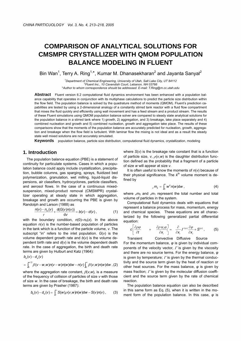
fied computational geometry we have used a 2-D ap-proximation of a stirred tank. This allows testing of the PBE within Fluent simply without solving a complicated 3-D flow problem with rotating grids typical of a stirred tank. The 2-D grid developed is given in Fig. 1.

Fig. 1 Grid for 2-D simulation of well mixed stirred tank.

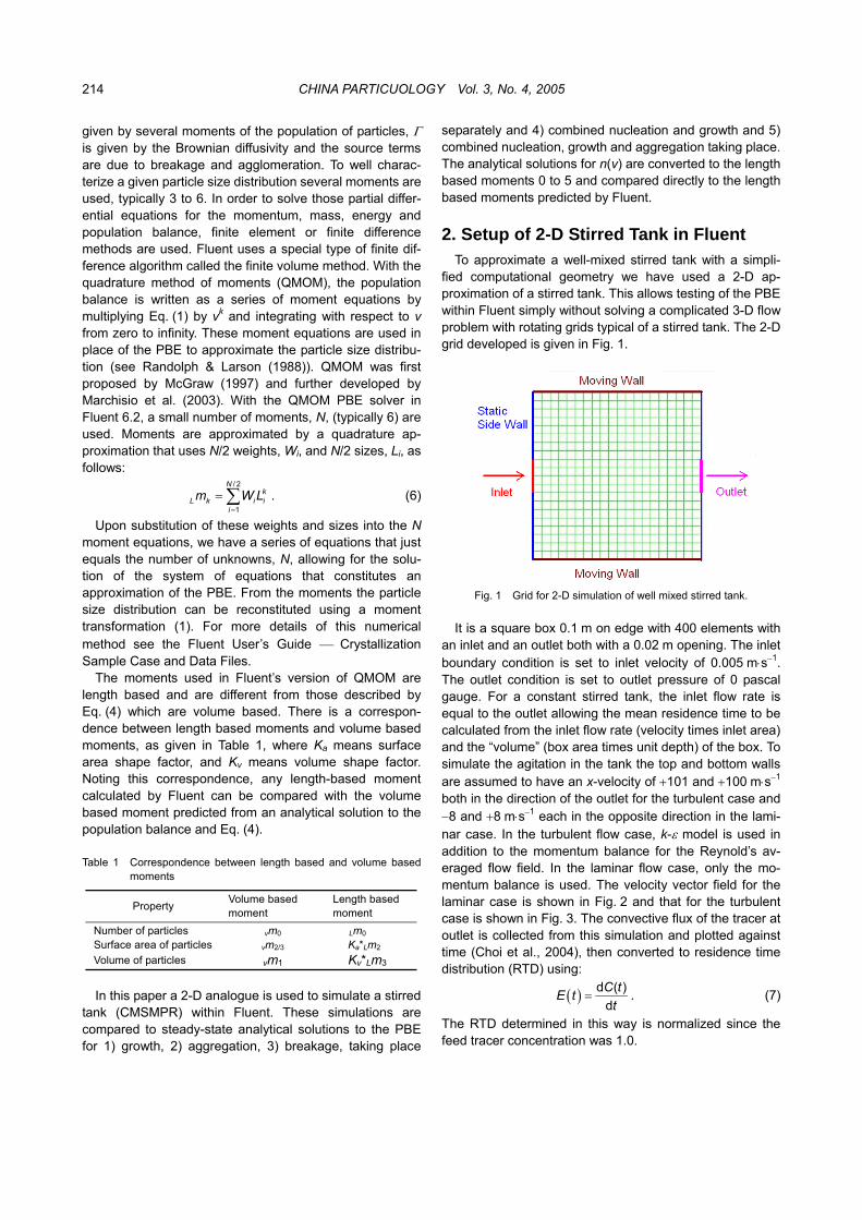
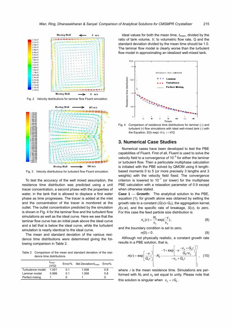
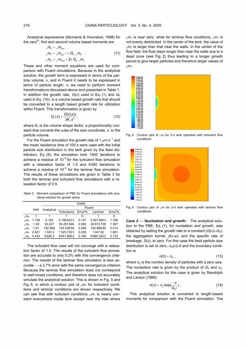
It is a square box 0.1 m on edge with 400 elements with an inlet and an outlet both with a 0.02 m opening. The inlet boundary condition is set to inlet velocity of 0.005 m⋅s−1. The outlet condition is set to outlet pressure of 0 pascal gauge. For a constant stirred tank, the inlet flow rate is equal to the outlet allowing the mean residence time to be calculated from the inlet flow rate (velocity times inlet area) and the “volume” (box area times unit depth) of the box. To simulate the agitation in the tank the top and bottom walls are assumed to have an x-velocity of +101 and +100 m⋅s−1 both in the direction of the outlet for the turbulent case and −8 and +8 m⋅s−1 each in the opposite direction in the lami-nar case. In the turbulent flow case, k-ε model is used in addition to the momentum balance for the Reynold’s av-eraged flow field. In the laminar flow case, only the mo-mentum balance is used. The velocity vector field for the laminar case is shown in Fig. 2 and that for the turbulent case is shown in Fig. 3. The convective flux of the tracer at outlet is collected from this simulation and plotted against time (Choi et al., 2004), then converted to residence time distribution (RTD) using:

( ) d ( )dC tE t

t= . (7)

The RTD determined in this way is normalized since the feed tracer concentration was 1.0.

Wan, Ring, Dhanasekharan & Sanyal: Comparison of Analytical Solutions for CMSMPR Crystallizer 215

Fig. 2 Velocity distributions for laminar flow Fluent simulation.

Fig. 3 Velocity distributions for turbulent flow Fluent simulation.

To test the accuracy of the well mixed assumption, the residence time distribution was predicted using a unit tracer concentration, a second phase with the properties of water, in the tank that is allowed to displace a first water phase as time progresses. The tracer is added at the inlet and the concentration of the tracer is monitored at the outlet. The outlet concentration predicted by the simulation is shown in Fig. 4 for the laminar flow and the turbulent flow simulations as well as the ideal curve. Here we see that the laminar flow curve has an initial peak above the ideal curve and a tail that is below the ideal curve, while the turbulent simulation is nearly identical to the ideal curve.

The mean and standard deviation of the various resi-dence time distributions were determined giving the fol-lowing comparison in Table 2.

Table 2 Comparison of the mean and standard deviation of the resi-dence time distributions

tmean (V/Q) Error/% Std.Deviation/tmean Error%

Turbulence model 1.001 0.1 1.008 0.8 Laminar model 0.999 0.1 1.058 5.8 Perfect mixing 1 0 1 0

Ideal values for both the mean time, tmean, divided by the ratio of tank volume, V, to volumetric flow rate, Q and the standard deviation divided by the mean time should be 1.0. The laminar flow model is clearly worse than the turbulent flow model in approximating an idealized well-mixed tank.

Res

iden

ce ti

me

dist

ribut

ion

Fig. 4 Comparison of residence time distributions for laminar (□) and turbulent (•) flow simulations with ideal well-mixed tank (-) with the Equation, E(t)=exp(−t/τ), τ =V/Q.

Time/s

3. Numerical Case Studies Numerical cases have been developed to test the PBE

capabilities of Fluent. First of all, Fluent is used to solve the velocity field to a convergence of 10−5 for either the laminar or turbulent flow. Then a particulate multiphase calculation is initiated with the PBE solved by QMOM using 6 length- based moments 0 to 5 (or more precisely 3 lengths and 3 weights) with the velocity field fixed. The convergence criterion is lowered to 10−7 (or lower) for the multiphase PBE calculation with a relaxation parameter of 0.9 except when otherwise stated. Case 1 Growth: The analytical solution to the PBE, equation (1), for growth alone was obtained by setting the growth rate to a constant (G(v)=G0), the aggregation kernel, β(v,w), and the specific rate of breakage, S(v), to zero. For this case the feed particle size distribution is

0in

0 0

( ) exp( )N vn vv v

−= , (8)

and the boundary condition is set to zero, (0) 0n = . (9)

Although not physically realistic, a constant growth rate results in a PBE solution, that is,

0 0

0 00

0 0 0

1 exp( ) exp

v GvG vvn v N

G v G

ττ

τ τ

− +− + − − = − − +

, (10)

where τ is the mean residence time. Simulations are per-formed with N0 and v0 set equal to unity. Please note that this solution is singular when 0 0v Gτ= .

CHINA PARTICUOLOGY Vol. 3, No. 4, 2005 216

Analytical expressions (Nicmanis & Hounslow, 1998) for the zeroth, first and second volume based moments are

1

0 0,in

1 1,in 0 0

2 2,in 02

v v

v v v

v v v

m mm m G mm m G m

τ

τ

=

= +

= +

. (11)

These and other moment equations are used for com-parison with Fluent simulations. Because in the analytical solution, the growth term is expressed in terms of the par-ticle volume, v, and in Fluent it needs to be expressed in terms of particle length, x, we need to perform moment transformations discussed above and presented in Table 1. In addition the growth rate, G(v) used in Eq. (1) and G0

used in Eq. (10), is a volume based growth rate that should be converted to a length based growth rate for utilization within Fluent. This transformation is given by

2

( ( ))( )3L

v

G v xG xK x

= , (12)

where Kv is the volume shape factor, a proportionality con-stant that converts the cube of the size coordinate, x, to the particle volume.

For the Fluent simulation the growth rate of 1 µm⋅s−1 and the mean residence time of 100 s were used with the initial particle size distribution in the tank given by the feed dis-tribution, Eq. (8), the simulation took 1600 iterations to achieve a residue of 10−9 for the turbulent flow simulation with a relaxation factor of 1.0 and 4000 iterations to achieve a residue of 10−9 for the laminar flow simulation. The results of these simulations are given in Table 3 for both the laminar and turbulent flow simulations with a re-laxation factor of 0.9.

Table 3 Moment comparison of PBE for Fluent simulations with ana-lytical solution for growth alone

Outlet Fluent

Inlet Analytical Turbulence Error/% Laminar Error/%

Lm0 1 1 1 0 1 0 Lm1 1.108 5.183 5.190 6333 0.147 5.091 3844 1.768Lm2 1.39 30.227 30.251 846 0.082 29.813 738 1.367Lm3 1.91 192.896 193.028 59 0.069 192.868 99 0.014Lm4 2.821 1 323.3 1 325.7223 0.206 1 347.62 1.861Lm5 4.423 9 626.3 9 641.8662 0.165 9 985.3242 3.733

The turbulent flow case will not converge with a relaxa-tion factor of 1.0. The results of the turbulent flow simula-tion are accurate to only 0.2% with this convergence crite-rion. The results of the laminar flow simulation is less ac-curate a 3.7% error with the same convergence criterion. Because the laminar flow simulation does not correspond to well-mixed conditions, and therefore does not accurately simulate the analytical solution. This is shown in Fig. 5 and Fig. 6, in which a contour plot of Lm1 for turbulent condi-tions and laminar conditions are shown respectively. We can see that with turbulent conditions Lm1 is nearly con-stant everywhere inside tank except near the inlet where

Lm1 is near zero, while for laminar flow conditions, Lm1 is not evenly distributed. In the center of the tank, the value of Lm1 is larger than that near the walls. In the center of the flow field, the fluid stays longer than near the walls due to a dead zone (see Fig. 2) thus leading to a longer growth period to give larger particles and therefore larger values of Lm1.

Fig. 5 Contour plot of Lm1 for 2-d tank operated with turbulent flow

conditions.

Fig. 6 Contour plot of Lm1 for 2-d tank operated with laminar flow

conditions.

Case 2 Nucleation and growth: The analytical solu-tion to the PBE, Eq. (1), for nucleation and growth, was obtained by setting the growth rate to a constant (G(v)=G0), the aggregation kernel, β(v,w), and the specific rate of breakage, S(v), to zero. For this case the feed particle size distribution is set to zero, nin(v)=0 and the boundary condi-tion is

0(0)n n= , (13) where n0 is the number density of particles with a zero size. The nucleation rate is given by the product of G0 and n0. The analytical solution for this case is given by Randolph and Larson (1988):

00

( ) exp( )xn x nG τ−

= , (14)

This analytical solution is converted to length-based moments for comparison with the Fluent simulation. The

Wan, Ring, Dhanasekharan & Sanyal: Comparison of Analytical Solutions for CMSMPR Crystallizer 217

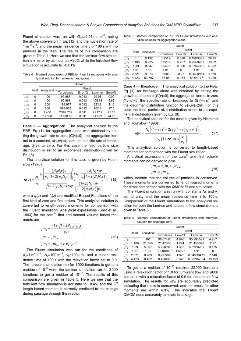
Fluent simulation was run with GL-0=0.01 mm⋅s−1, noting the above conversion in Eq. (12) and the nucleation rate of 1 m−3⋅s−1, and the mean residence time τ of 100 s with no particles in the feed. The results of this comparison are given in Table 4. Here we see that the laminar flow simula-tion is in error by as much as ~25% while the turbulent flow simulation is accurate to ~0.01%.

Table 4 Moment comparison of PBE for Fluent simulations with ana-lytical solution for nucleation and growth

Outlet Fluent

Inlet Analytical Turbulence Error/% Laminar Error/%

Lm0 0 100 99.987 0.013 99.98 0.02 Lm1 0 100 99.988 0.012 105.68 5.68 Lm2 0 200 199.977 0.012 223.2 11.6 Lm3 0 600 599.933 0.012 702.3 17.5 Lm4 0 2 400 2 399.732 0.011 2 917.2 21.55Lm5 0 12 000 11 998.66 0.011 14 982 24.85

Case 3 Aggregation: The analytical solution to the PBE, Eq. (1), for aggregation alone was obtained by set-ting the growth rate to zero (G(v)=0), the aggregation ker-nel to a constant, β(v,w)=β0, and the specific rate of break-age, S(v), to zero. For this case the feed particle size distribution is set to an exponential distribution given by Eq. (8).

The analytical solution for this case is given by Houn-slow (1990):

( )

( )( )

( )( )

( ) ( )( )

0 0 0 00 1

0 0 0 0 0 00

0 0 00 0

0 0 0

1 2 1 2

11 2 exp

1 2

N v N vI I

v N v NNn vv N v

NN v

β τ β τβ τ β τ

β τβ τ

β τ

− −+

+ + = +

+ +

, (15)

where I0(z) and I1(z) are modified Bessel Functions of the first kind of zero and first orders. This analytical solution is converted to length-based moments for comparison with the Fluent simulation. Analytical expressions (Smit et al., 1993) for the zeroth, first and second volume based mo-ments are

1

0 0,in0

0

1 1,in

22 2,in 0

1 1 2 vv

v v

v v v

mm

m m

m m m

β τβ τ

τ β

− + +=

=

= +

. (16)

The Fluent simulation was run for the conditions of β0=1 m4⋅s−1, N0=100 m−3, v0=100 µm, and a mean resi-dence time of 100 s with the relaxation factor set to 0.9. The turbulent simulation ran for 1000 iterations to get to a residue of 10−9 while the laminar simulation ran for 3000 iterations to get a residue of 10−10. The results of this comparison are given in Table 5. Here we see that the turbulent flow simulation is accurate to ~0.4% and the 3rd length based moment is correctly predicted to not change during passage through the reactor.

Table 5 Moment comparison of PBE for Fluent simulations with ana-lytical solution for aggregation alone

Outlet Fluent

Inlet AnalyticalTurbulence Error/% Laminar Error/%

Lm0 1 0.132 0.131 9 0.076 0.159 3889 20.75Lm1 1.108 0.225 0.225 6 0.267 0.254 9767 13.32Lm2 1.39 0.547 0.549 0 0.366 0.576 4962 5.392Lm3 1.91 1.91 1.91 0 1.91 0 Lm4 2.821 9.073 9.093 0.22 8.967 8564 1.159Lm5 4.423 53.797 53.88 0.154 53.049 77 1.389

Case 4 Breakage: The analytical solution to the PBE, Eq. (1), for breakage alone was obtained by setting the growth rate to zero (G(v)=0), the aggregation kernel to zero, β(v,w)=0, the specific rate of breakage to S(v)=v s−1 and the daughter distribution function to ρ(v,w)=2/w. For this case the feed particle size distribution is set to an expo-nential distribution given by Eq. (8).

The analytical solution for the case is given by Nicmanis and Hounslow (1998):

( ) ( )( )

( )

20 0 0

00

1 2 1( )

1 exp

N v v v vn v

vv vv

τ τ τ

τ

+ + + + =

+

. (17)

This analytical solution is converted to length-based moments for comparison with the Fluent simulation.

Analytical expressions of the zeroth and first volume moments can be derived to give

0 1

1 1,in

v v v

v v

m m mm m

τ= +

=0,in , (18)

which indicate that the volume of particles is conserved. These moments are converted to length-based moments for direct comparison with the QMOM Fluent simulation.

The Fluent simulation was run with constants N0 and v0 set to unity and the mean residence time τ to 100 s. Comparison of the Fluent simulations to the analytical so-lution for both the laminar and turbulent flow simulations is given in Table 6.

Table 6 Moment comparison of Fluent simulations with analytical solution for breakage only

Outlet Fluent

Inlet AnalyticalTurbulence Error/% Laminar Error/%

Lm0 1 101 96.074 96 4.876 95.993 599 4.957Lm1 1.108 21.758 21.476 35 1.294 21.155 323 2.77 Lm2 1.39 5.807 5.728 288 1.355 5.622 628 7 3.175Lm3 1.91 1.91 1.910 0003 1.6E−5 1.91 0 Lm4 2.821 0.789 0.797 085 1.025 0.845 39419 7.148Lm5 4.423 0.422 0.420 623 0.326 0.502 84964 19.159

To get to a residue of 10−10 required 22000 iterations using a relaxation factor of 1.0 for turbulent flow and 9000 iterations with a relaxation factor of 0.9 for the laminar flow simulation. The results for Lm3 are accurately predicted indicating that mass is conserved, and the errors for other moments are within 4.9%. This indicates that Fluent QMOM does accurately simulate breakage.

CHINA PARTICUOLOGY Vol. 3, No. 4, 2005 218

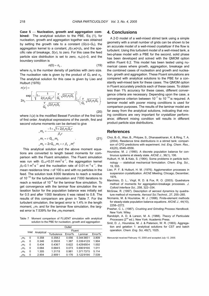
Case 5 Nucleation, growth and aggregation com-bined: The analytical solution to the PBE, Eq. (1), for nucleation, growth and aggregation together was obtained by setting the growth rate to a constant (G(v)=G0), the aggregation kernel to a constant, β(v,w)=β0, and the spe-cific rate of breakage, S(v), to zero. For this case the feed particle size distribution is set to zero, nin(v)=0, and the boundary condition is

n0(0)n = , (19) where n0 is the number density of particles with zero size. The nucleation rate is given by the product of G0 and n0. The analytical solution for this case is given by Liao and Hulburt (1976): ( )

0 0 020 0 0 0

00

0 0 00

1exp 1 22

22

n v

v n Gn G G vn v Gn G

G

ββ τ

ββ

=

− +

1 0 0 02 ,I n G

(20) where I1(z) is the modified Bessel Function of the first kind of first order. Analytical expressions of the zeroth, first and second volume moments can be derived to give

1

0 0 00

0

1 0 02

2 0 1 0

1 1 2

2

v

v v

v v

n Gm

m G mm G m v m

β τβ τ

τ

τ τ β

− + +=

=

= +

. (21)

This analytical solution and the above moment equa-tions are converted to length based moments for com-parison with the Fluent simulation. The Fluent simulation was run with Gv-0=0.01 mm3⋅s−1, the aggregation kernel β0=0.1 m4⋅s−1 and the nucleation rate of 0.01 m−3⋅s−1, the mean residence time τ of 100 s and with no particles in the feed. The solution took 8000 iterations to reach a residue of 10−10 for the turbulent simulation and 7000 iterations to reach a residue of 10−9 for the laminar flow simulation. To get convergence with the laminar flow simulation the re-laxation factor for the population balance was initially set for 0.5 and after 1000 iterations it was raised to 0.8. The results of this comparison are given in Table 7. For the turbulent simulation, the largest error is 1.4% in the length moment, Lm1 and for the laminar flow simulation, the larg-est error is 7.539% for the Lm5 moment.

Table 7 Moment comparison of FLUENT simulation with analytical solution to the PBE for nucleation, growth and aggregation

Outlet Fluent

Inlet Analytical Turbulence Error/% Laminar Error/%

Lm0 0 0.358 0.358 2 0.056 0.344 3651 3.809Lm1 0 0.346 0.350 8 1.387 0.339 4129 1.904Lm2 0 0.434 0.436 7 0.622 0.429 6504 1.002Lm3 0 0.684 0.684 5 0.073 0.690 9166 1.011Lm4 0 1.305 1.317 8 0.981 1.371 7375 5.114Lm5 0 2.904 2.909 1 0.176 3.122 9196 7.539

4. Conclusions A 2-D model of a well-mixed stirred tank using a simple

geometry with a small number of grids can be shown to be an accurate model of a well-mixed crystallizer if the flow is turbulent. Using this turbulent model of a well-mixed tank, a two-phase model with a PBE for the second, solid phase has been developed and solved with the QMOM option within Fluent 6.2. This model has been tested using nu-merical cases where growth, aggregation, breakage and the combined cases of nucleation and growth and nuclea-tion, growth and aggregation. These Fluent simulations are compared with analytical solutions to the PBE for a con-stantly well-mixed tank for these cases. The QMOM option in Fluent accurately predicts each of these cases. To obtain less than 1% accuracy for these cases, different conver-gence criteria are necessary. Depending upon the case, a convergence criterion between 10−7 to 10−14 is required. A laminar model with poorer mixing conditions is used for comparison purposes. The results of the laminar model are far away from the analytical solutions, indicating that mix-ing conditions are very important for crystallizer perform-ance; different mixing condition will results in different product particle size distributions.

References Choi, B.-S., Wan, B., Philyaw, S., Dhanasekharan, K. & Ring, T. A.

(2004). Residence time distributions in a stirred tank: compari-son of CFD predictions with experiment. Ind. Eng. Chem. Res., 43(20), 6548-6556.

Hounslow, M. J. (1990). A discrete population balance for con-tinuous systems at steady state. AIChE J., 36(1), 106.

Hulburt, H. M. & Katz, S. (1964). Some problems in particle tech-nology statistical mechanical formulation. Chem. Eng. Sci., 19, 555.

Liao, P. F. & Hulburt, H. M. (1976). Agglomeration processes in suspension crystallization. AIChE Meeting, Chicago, December, 1976.

Marchisio, D. L., Virgil, R. D. & Fox, R. O. (2003). Quadrature method of moments for aggregation-breakage processes. J. Colloid Interface Sci., 258, 322-334.

McGraw, R. (1997). Description of aerosol dynamics by quadra-ture method of moments. Aerosol Sci.Technol., 27, 255-265.

Nicmanis, M. & Hounslow, M. J. (1998). Finite-element methods for steady-state population balance equations. AIChE J., 44(10), 2258-2272.

Prasher, C. L. (1987). Crushing and Grinding Process Handbook. New York: Wiley.

Randolph, A. D. & Larson, M. A. (1988). Theory of Particulate Processes (2nd ed.). New York: Academic Press.

Smit, D. J., Hounslow, M. J. & Paterson, W. R. (1993). Aggrega-tion and gelation 1: analytical solutions for CST and batch operation. Chem. Eng. Sci, 49(7), 1025.

Manuscript received February 15, 2005 and accepted July 12, 2005.