Comparison of a Fluid and a Solid Approach for the ...cervera.rmee.upc.edu/papers/2014-SRI-comparison-no.pdf · Comparison of a Fluid and a Solid Approach for the Numerical Simulation

www.steel-research.de

FULL

PAPER

Comparison of a Fluid and a Solid Approach forthe Numerical Simulation of Friction Stir Weldingwith a Non‐Cylindrical Pin

Philippe Bussetta,� Narges Dialami, Romain Boman, Michele Chiumenti,Carlos Agelet de Saracibar, Miguel Cervera, and Jean‐Philippe Ponthot

Friction stir welding (FSW) process is a solid‐state joining process during which materials tobe joined are not melted. As a consequence, the heat‐affected zone is smaller and the qualityof the weld is better with respect to more classical welding processes. Because of extremelyhigh strains in the neighborhood of the tool, classical numerical simulation techniques haveto be extended in order to track the correct material deformations. The ArbitraryLagrangian–Eulerian (ALE) formulation is used to preserve a good mesh quality throughoutthe computation. With this formulation, the mesh displacement is independent from thematerial displacement. Moreover, some advanced numerical techniques such as remeshingor a special computation of transition interface is needed to take into account non‐cylindricaltools. During the FSW process, the behavior of the material in the neighborhood of the tool isat the interface between solid mechanics and fluid mechanics. Consequently, a numericalmodel of the FSW process based on a solid formulation is compared to another one based ona fluid formulation. It is shown that these two formulations essentially deliver the sameresults in terms of pressures and temperatures.

1. Introduction and State of the Art in FSW

Friction stir welding (FSW) is a new method of welding in

solid state, created and patented by The Welding Institute

(TWI) in 1991.[1] In FSW a cylindrical, shouldered tool with

a profiled probe, also called pin, is rotated and slowly

plunged into the joint line between two pieces of sheet or

platematerial, which are butted together. The parts have to

be clamped onto a backing bar in a manner that prevents

the abutting joint faces from being forced apart. Once

the probe has been completely inserted, it is moved with

a small tilt angle in the welding direction. The shoulder

applies a pressure on the material to constrain the

plasticised material around the probe tool. Due to the

advancing and rotating effect of the probe and shoulder of

the tool along the seam, an advancing side and a retreating

[�] P. Bussetta, R. Boman, J. -P. PonthotDepartment of Aerospace and Mechanical Engineering, Non LinearComputational Mechanics, University of Liege, Building B52/3, Chemindes Chevreuils, 1 B-4000, Liege, BelgiumEmail: [email protected]. Dialami, M. Chiumenti, C. Agelet de Saracibar, M. CerveraInternational Centre for Numerical Methods in Engineering (CIMNE),Universidad Politecnica de Cataluna, Campus Norte UPC 08034,Barcelona, Spain

DOI: 10.1002/srin.201300182

� 2013 WILEY-VCH Verlag GmbH & Co. KGaA, Weinheim

side are formed and the softened and heatedmaterial flows

around the probe to its backside where the material is

consolidated to create a high-quality solid-state weld

(see Figure 1). The maximum temperature reached is of

the order of 80% of the melting temperature. Despite the

simplicity of the procedure, the mechanisms behind

the process and the material flow around the probe tool

are very complex. The material is extruded around the

rotating tool and a vortex flow field near the probe due to

the downward flow is induced by the probe thread. The

process can be regarded as a solid phase keyhole welding

technique since a hole to accommodate the probe is

generated, then filled during the welding sequence. The

material flow depends onwelding process parameters, such

as welding and rotation speed, pressure, etc., and on the

characteristics of the tools, such as materials, design, etc.

The first applications of FSW have been in aluminum

fabrications. Aluminum alloys that are difficult to weld

using conventional welding techniques, are successfully

welded using FSW. The weld quality is excellent, with none

of the porosity that can arise in fusion welding, and the

mechanical properties are at least as good as the best

achievable by fusion welding. Being a solid-state welding

process, the structure in the weld nugget is free of

solidifying segregation, being suitable for welding of

composite materials. The process is environmentally

friendly, because no fumes or spatter are generated, and

steel research int. 84 (2013) No. 9999 1

pinshoulder

weldedzone

advancingside

retreatingside

pinshoulder

(a) (b)

Figure 1. Scheme of the FSW process. a) General view. b) View of the too.


FULL

PAPER

there is no arc glare or reflected laser beams with which to

contend. Another major advantage is that, by avoiding the

creation of a molten pool, which shrinks significantly

on re-solidification, the distortion after welding and the

residual stresses are low. With regard to joint fit up,

the process can accommodate a gap of up to 10% of the

material thickness without impairing the quality of the

resulting weld. As far as the rate of processing is concerned,

for materials of 2mm thickness, welding speeds of up to

2mmin�1 can be achieved, and for 5mm thickness up to

0.75mmin�1. Recent tool developments are confidently

expected to improve on these figures.

FSW has been used to weld all wrought aluminum

alloys, across the AA-2xxx, AA-5xxx, AA-6xxx, and AA-7xxx

series of alloys, some of which are bordering on being

classed as virtually unweldable by fusion welding techni-

ques. The process can also weld dissimilar aluminum

alloys, whereas fusion welding may result in the alloying

elements from the different alloys interacting to form

deleterious intermetallics through precipitation during

solidification from the molten weld pool. FSW can also

make hybrid components by joining dissimilar materials

such as aluminum andmagnesium alloys. The thicknesses

of AA-6082-T6 that have so far been welded have ranged

from 1.2 to 50mm in a single pass, to more than 75mm

when welding from both sides. Welds have also been

made in pressure die cast aluminum material without

any problems from pockets of entrapped high pressure

gas, which would violently disrupt a molten weld pool

encountering them.

The original application for FSWwas thewelding of long

lengths of material in the aerospace, shipbuilding, and

railway industries. Examples include large fuel tanks and

other containers for space launch vehicles, cargo decks for

high-speed ferries, and roofs for railway carriages. FSW is

used already in routine, as well as in critical applications,

for the joining of structural components made of alumi-

num and its alloys. Indeed, it has been convincingly

demonstrated that the process results in strong and ductile

joints, sometimes in systems, which have proved difficult

using conventional welding techniques. The process is

2 steel research int. 84 (2013) No. 9999

most suitable for components, which are flat and long

(plates and sheets) but can be adapted for pipes, hollow

sections, and positional welding.

The computational modeling of FSW processes is a

complex task and it has been a research topic of increasing

interest in computational mechanics during the last

decades.

Thermal models for the numerical simulation of FSW

processes were used byMcClure et al.,[2] Colegrove et al.,[3]

Khandkar and Khan,[4] and Khandkar et al.[5]

Bendzsak et al.[6,7] used the Eulerian code Stir3D to

model the flow around a FSW tool, including the tool

thread and tilt angle in the tool geometry and obtaining

complex flow patterns. The temperature effects on the

viscosity were neglected.

Dong et al.[8] developed a simplified model for the

numerical simulation of FSW processes, taking into

account both the friction heating and plastic work in

the modeling of the heat flow phenomena, predicting the

development of a plastic strain around the weld zone in

the initial stage of welding. However, they did not consider

the longitudinal movement of the tool.

Xu et al.[9] and Xu and Deng[10] developed a 3D finite

element procedure to simulate the FSW process using

the commercial finite element method (FEM) software

ABAQUS, focusing on the velocity field, the material

flow characteristics, and the equivalent plastic strain

distribution. The authors used an Arbitrary Lagrangian–

Eulerian (ALE) formulation with adaptive meshing and

consider large elasto-plastic deformations and tempera-

ture-dependent material properties. However, the authors

did not perform a fully coupled thermo-mechanical

simulation, superimposing the temperature map obtained

from the experiments as a prescribed temperature field to

perform the mechanical analysis. The numerical results

were compared to experimental data available, showing

a reasonable good correlation between the equivalent

plastic strain distributions and the distribution of the

microstructure zones in the weld.

Ulysse[11] presented a fully coupled 3D FEM visco-

plastic model for FSW of thick aluminum plates using the



FULL

PAPER

commercial FEM code FIDAP. The author investigated the

effect of tool speeds on the process parameters. It was

found that a higher translational speed leads to a higher

welding force, while increasing the rotation speed has

the opposite effect. Reasonable agreement between the

predicted and the measured temperature was obtained

and the discrepancies were explained by an inadequate

representation of the constitutive behavior of the material

for the wide ranges of strain-rate, temperatures, and

strains typically found during FSW.

Askari et al.[12] used the CTH hydrocode coupled to an

advection–diffusion solver for the energy balance equa-

tion. The CTH code, developed by Sandia National

Laboratories, uses the finite volume method to discretize

the domain. The elastic response was taken into account in

this case. The results proved encouraging with respect to

gaining an understanding of the material flow around the

tool. However, simplified friction conditions were used.

Chen and Kovacevic[13] developed a 3D FEM model to

study the thermal history and thermo-mechanical phe-

nomena in the butt-welding of aluminum alloy AA-6061-

T6 using the commercial FEM code ANSYS. Their model

incorporated the mechanical reaction between the tool

and the weld material. Experiments were conducted and

an X-ray diffraction technique was used to measure

the residual stress in the welded plate. The welding

tool (i.e., the shoulder and pin) in the FEM model

was modeled as a heat source, with the nodes moved

forward at each computational time step. This simple

model severely limited the accuracy of the stress and force

predictions.

Colegrove et al.[3,14] used the commercial Computa-

tional Fluid Dynamics (CFD) software FLUENT for a 2D

and 3D numerical investigation on the influence of pin

geometry during FSW, comparing different pin shapes in

terms of material flow and welding forces on the basis of

both a stick and a slip boundary condition at the tool/

work-piece interface. In spite of the good obtained results,

the accuracy of the analysis was limited by the assumption

of isothermal conditions. Seidel and Reynolds[15] also used

the CFD commercial software FLUENT to model the 2D

steady-state flow around a cylindrical tool.

Schmidt and Hattel[16] presented the development of a

3D fully coupled thermo-mechanical finite element model

in ABAQUS/Explicit using the ALE formulation. The

flexibility of the FSW machine was taken into account

by connecting the rigid tool to a spring. The work-piece

was modeled as a cylindrical volume with inlet and outlet

boundary conditions. A rigid back-plate was used. The

contact forces weremodeled using a Coulomb friction law,

and the surface was allowed to separate. Heat generated

by friction and plastic deformation was considered. The

simulation modeled the dwell and weld phases of the

process.

An ALE formulation for the numerical simulation of

FSW processes was also used by Zhao,[17] Guerdoux,[18]

and Assidi et al.[19]


Nikiforakis[20] used a finite difference method to model

the FSW process. Despite the fact that he was only

presenting 2D results, the model proposed had the

advantage of minimizing the calibration of model param-

eters, taking into account amaximum of physical effects. A

transient and fully coupled thermo-fluid analysis was

performed. The rotation of the tool was handled through

the use of the overlapping gridmethod. A rigid-viscoplastic

material law was used and sticking contact at the tool work

piece interface was assumed. Hence, heating was due to

plastic deformation only.

Heurtier et al.[21] used a 3D semi-analytical coupled

thermomechanical FE model to simulate FSW processes.

The model uses an analytical velocity field and considers

heat input from the tool shoulder and plastic strain of

the bulk material. Trajectories, temperature, strain, strain

rate fields, and micro-hardness in various weld zones were

computed and compared to experimental results obtained

on an AA 2024-T351 alloy FSW joint.

Buffa et al.[22] using the commercial finite element

software DEFORM-3D, proposed a 3D Lagrangian, implic-

it, coupled thermo-mechanical numerical model for the

simulation of FSW processes, using a rigid-viscoplastic

material description and a continuum assumption for

the weld seam. The proposed model is able to predict the

effect of process parameters on process variables, such as

the temperature, strain, and strain rate fields, as well as

material flow and forces. A reasonable good agreement

between the numerically predicted results, on forces

and temperature distribution, and experimental data

was obtained. The authors found that the temperature

distribution about the weld line is nearly symmetric

because the heat generation during FSW is dominated by

rotating speed of the tool, which is much higher than the

advancing speed. On the other hand, the material flow in

the weld zone is non-symmetrically distributed about

the weld line because the material flow during FSW is

mainly controlled by both advancing and rotating speeds.

De Vuyst et al.[23–26] used the coupled thermo-

mechanical finite element code MORFEO to simulate

the flow around simplified tool geometries for FSW

process. The rotation and advancing speed of the tool

were modeled using prescribed velocity fields. An attempt

to consider features associated to the geometrical details

of the probe and shoulder, which had not been discretized

in the finite element model in order to avoid very large

meshes, was taken into account using additional special

velocity boundary conditions. In spite of that, a mesh of

roughly 250 000 nodes and almost 1.5 million of linear

tetrahedral elements was used. A Norton–Hoff rigid-

viscoplastic constitutive equation was considered, with

averaged values of the consistency and strain rate

sensitivity constitutive parameters determined from hot

torsion tests performed over a range of temperatures

and strain rates. The computed streamlines were com-

pared with the flow visualization experimental results

obtained using copper marker material sheets inserted



FULL

PAPER
transversally or longitudinally to the weld line. The
simulation results correlated well when compared to

markers inserted transversely to the welding direction.

However, when compared to a marker inserted along the

weld centreline only qualitative results could be obtained.

The correlationmay be improved bymodeling the effective

weld thickness of the experiment, using a more realistic

material model, for example, by incorporating a yield

stress or temperature dependent properties, refine velocity

boundary conditions or further refining the mesh in

specific zones, such as for instance, under the probe. The

authors concluded that it is essential to take into account

the effects of the probe thread and shoulder thread in order

to get realistic flow fields.

Shercliff et al.[27] developed microstructural models for

FSW of 2000 series aluminum alloys.

Lopez et al.[28] and Agelet de Saracibar et al.[29]

developed numerical algorithms to optimize material

model and FSW process parameters using neural net-

works. They proposed a new model for the dissolution of

precipitates in fully hardened aluminum alloys and they

optimized the master curve and the effective activation

energy. Furthermore, they developed an algorithm to

optimize the advancing and rotation speed, taking as weld

quality criteria the minimization of the maximum

hardness drop at the transversal section under the pin.

Santiago et al.[30] developed a simplified computational

model taking into account the real geometry of the tool,

i.e., the probe thread, and using an ALE formulation. They

considered also a simplified friction model to take into

account different slip/stick conditions at the pin shoulder/

work-piece interface.

Agelet de Saracibar et al.,[31–33] Chiumenti et al.,[34] and

Dialami et al.[35] used a sub-grid scale finite element

stabilized mixed velocity/pressure/temperature formula-

tion for coupled thermo-rigid-plasticmodels, using Eulerian

and ALE formalisms, for the numerical simulation of FSW

processes. They used ASGS and OSGS methods and quasi-

static sub-grid scales, neglecting the sub-grid scale pressure

and using the finite element component of the velocity in

the convective term of the energy balance equation.

Chiumenti et al.[34,36] and Dialami et al.,[35] developed

an apropos kinematic framework for the numerical

simulation of FSW processes. They considered a combi-

nation of ALE, Eulerian and Lagrangian descriptions at

different zones of the computational domain and they

proposed an efficient coupling strategy. Within this

approach, a Lagrangian formulation was used for the

pin, an ALE formulation was used at the stir zone of the

work-piece, and an Eulerian formulation was used in

the remaining part of the work-piece. The stir zone was

defined as a circular domain close to the pin. The finite

element mesh in the stir zone was rotating attached to the

pin. The resulting apropos kinematic setting efficiently

permitted to treat arbitrary pin geometries and facilitates

the application of boundary conditions. The formulation

was implemented in an enhanced version of the finite


element code COMET[37] developed by the authors at the

International Centre for Numerical Methods in Engineer-

ing (CIMNE).

Chiumenti et al.[36] used a novel stress-accurate FE

technology for highly non-linear analysis with incompres-

sibility constraints typically found in the numerical

simulation of FSW processes. They used a mixed linear

piece-wise interpolation for displacement, pressure, and

stress fields, respectively, resulting in an enhanced stress

field approximation, which enables for stress accurate

results in nonlinear computational mechanics.

This paper presents and compares two different numeri-

cal models of the FSW process, in the general case of a non-

cylindrical pin. The first model is based on a solid approach

written in terms of nodal positions and nodal temperatures.

The second model of FSW process is based on a fluid

approach written in terms of the velocity, the pressure, and

the temperature fields. Both models use advanced numeri-

cal techniques such as remeshing and the ALE formulation.

2. 2D Numerical Modeling of FSW Process

The FSW process is modeled in two dimensions under the

plane strain hypothesis. To model this welding process,

the displacement of the tool is split into an advancing

movement (actually assigned to the work-pieces but, in the

opposite direction) and a rotation (imposed to the tool).

In other words, the centre of the pin is fixed and a

constant velocity is imposed to the plates (see Figure 2a).

The tool is described by a classical Lagrangianmesh. Then,

in relation with the distance to the centre of the tool, three

zones of the plates are identified. In the closest zone

around the pin, the material is submitted to extremely

high strains. This region is called the thermo-mechanically

affected zone (TMAZ). Due to high deformations, the use of

a Lagrangian formalism would lead very quickly to mesh

entanglement. Thus, in this region, the ALE formulation

is employed. On top of this, the ALE formulation allows

the model to take into account non-circular pin shapes.

In this zone, the mesh has the same rotational speed as

the pin (red region in Figure 2b). In the furthest zone

from the tool, the gray zone in Figure 2b, the Eulerian

formulation is used. Thus in this region, the mesh is fixed.

The ring connecting region 1 and region 3 is a transition

zone (white region numbered 2 in Figure 2b). In such

a model, the quality of the mesh does not change

during the simulation except in the transition zone.

So, to overcome this problem, two different numerical

techniques are proposed (see Section 2.2.2).

2.1. Thermomechanical Formulation

The numerical models presented here are based on the

FEM. In this paper, two numerical formulations are


pin shoulder

weldedzone

advancingsideretreating

side

3 2 1

(a) (b)

Figure 2.Description of the FSWmodel. a) Scheme of the FSWmodel. A rotation is imposed to the pin (blue arrow) while the advancingvelocity of the pin is replaced by a velocity imposed to the plates in the opposite direction (red arrows). b) The different zones of themodel: ALE formulation is used on the red region (1), the transition zone corresponds to the white region (2), and the Eulerianformulation is applied on the gray region (3).


FULL

PAPER

compared. The first one is based on a solid mechanics

approach. It is written in terms of nodal positions and

temperatures. The second one is based on a fluid

mechanics approach. The equilibrium is written as a

function of nodal velocities, pressures, and temperatures.

2.1.1. Solid ApproachIn the solid approach, the finite element used are linear

quadrilaterals. The position and temperature fields are

computed at each node of the elements. The stresses

and the internal variables are computed at each

quadrature point of the element (4 Gauss points). To

overcome the locking phenomenon, the pressure is

considered constant over the element and computed

only at a central quadrature point. The thermomechan-

ical equations are split into a mechanical part and

a thermal part. At each time step, the mechanical

equations are first solved using a constant temperature

field. This temperature field is the one obtained at the

latest increment. Then, the thermal equations are solved

on the frozen resulting geometrical configuration

that has just been obtained.

2.1.2. Fluid ApproachThe fluid approach is based on a stabilized mixed linear

temperature–velocity–pressure finite element formula-

tion. This formulation is stabilized adopting the orthogo-

nal sub-grid scale method (OSS)[38–40] to solve both the

pressure instability induced by the incompressibility

constraint and the instabilities coming from the convective

term. A triangular mesh is used for the domain discretiza-

tion. The velocity, the pressure, and temperature fields are

computed at each node of the element. The deviatoric

stresses and the other internal variables are computed at

each quadrature point of the element. Finally, the coupled

thermo-mechanical problem is solved by means of a

staggered time-marching scheme where the thermal and


mechanical sub-problems are solved sequentially,

within the framework of the classical fractional step

methods.[41,42] This approach is exposed in more detail in

Refs.[34,35,38,40].

2.2. Numerical Simulation Strategy

2.2.1. Arbitrary Lagrangian–Eulerian FormulationIn region 1 and region 3 in Figure 2b, the ALE formulation

is used. Indeed, the Eulerian formulation (used in the

region 3) is a particular case of the ALE formulation. In the

ALE formalism, unlike in the Lagrangian case, which is

commonly used in solid mechanics, the mesh no longer

follows the material motion.[34,35,43–45] Consequently, a

new grid coordinate system R~x is defined and the

conservation laws able to describe the FSW process are

rewritten in terms of the new coordinates ~x :

Mass:

@r

@t

��~x

þ~c � ~rrþ r~r�~y¼ 0 ð1Þ

Momentum:

r@~y

@t

��~x

þ ð~c � ~rÞ~y !

¼ ~r� s þ r~b ð2Þ

Energy:

rCp@T

@t

��~x

þ~c � ~rT

!¼ Dmech � ~r� ~q ð3Þ

where r and Cp are the mass density and the specific heat

capacity, s is the Cauchy stress tensor, ~b is the specific



FULL

PAPER
body forces, T is the temperature, Dmech is the plastic
dissipation rate per unit of volume. The heat flux, ~q, is

defined according to the isotropic Fourier’s law as:

~q¼ �k~rT ð4Þ

The convective velocity ~c¼~y�~y�is the difference

between the material velocity ~y and the mesh velocity

~y�. Both the stress tensor, s, and the strain rate tensor, D,

are split into volumetric and deviatoric parts:

s ¼ pIþ S ð5Þ

D ¼ 1

3DvolIþ D ð6Þ

where p and S are the pressure and the stress deviator,

respectively. Similarly, Dvol¼ tr(D) and D¼ devðDÞ are

the volumetric and the deviatoric parts of the strain-rate

tensor, respectively.

The thermal boundary conditions are defined in terms

of the heat flux that flows through the boundaries by heat

convection and radiation. They are expressed by Newton

and radiation laws, respectively, as:

qconv ¼ hconvðT � T envÞ ð7Þ

qrad ¼ s0eðT4 � T4envÞ ð8Þ

where hconv is the heat transfer coefficient by convection,

s0 is the Stefan-Boltzmann constant and e is the emissivity

factor. Finally, Tenv is the surrounding environment

temperature.

The ALE formulations used in the two approaches are

different.

2.2.1.1. Solid Approach: The ALE formulation used in the

solid approach is described in more details in Refs.[43–45]

To simplify the solution procedure and remain

competitive against Lagrangian models, the system of

ALE equations (Equation 1–3) is solved using an operator-

split procedure. First, for each time step, the classical

Lagrangian thermomechanically coupled formalism is

used. During this Lagrangian step, the mesh sticks

to the material (~y� ¼~y;~c¼ 0) until an equilibrated

Lagrangian configuration is iteratively obtained. So, the

weak form of the governing equations which are solved

during this first step is defined over the current integration

domainV and its boundary @V (see Equation 9 and 10). Let

us assume that the boundary @V can be split into @Vs

and @Vu, being @V¼ @Vs[ @Vu such that tractions are

prescribed on @Vs while displacements are specified on

@Vu, respectively. In a similar way, boundary @V can be

also split into @Vq and @Vu such that @V¼ @V[ @Vu where

fluxes (on @Vq) and temperatures (on @Vu) are prescribed


for the heat transfer analysis

ZV

rd2~u

dt2� d~u

� �dV ¼

ZV

ðr~b � d~uÞdV �ZV

ðs : ~rd~uÞdV

þZ@Vs

ð~t � d~uÞdSð9Þ

ZV

rCpdT

dtdT

� �dV þ

ZV

k~rT :~rðdTÞh i

dV

¼ZV

DmechdTð ÞdV �Z@Vq

ðqconv þ qradÞdT½ �dS ð10Þ

where d~u and dT are the test functions of the displacement

and temperature fields. ~t is prescribed tractions on the

boundary domain @Vs.

The second step, also called the Eulerian step, is divided

into two substeps: first the nodes of themesh are relocated

to a more suitable position, thus defining a newmesh with

the same topology and the mesh velocity ~y�. In the case

of region 1 and region 3, the position of the relocated

nodes is known because the mesh velocity of these regions

is imposed. Then, the unknowns and the internal variables

are transferred from the old mesh to the new one.[45]

2.2.1.2. Fluid Approach: The ALE formulation used in

the fluid model is not based on a operator-split like in

the formulation presented for the solid approach. In this

fully coupled formulation,[34,35] the equilibrium state is

computed at each time increment without remeshing and

remapping steps. The system of equations solved includes

the convective terms due to the velocity of the mesh

relative to the material. In the TMAZ, region 1 in Figure 2b,

the velocity of the mesh is imposed and the velocity and

the pressure of the material are directly computed. In the

case of the Eulerian formulation (region 3 in Figure 2b),

the mesh does not move during the computation. The

following assumptions are considered for the numerical

simulation of the FSW process (more detail can be found

in Refs.[34,35]):

�
The flow is assumed to be incompressible as the
volumetric changes including thermal deformation are

found to be negligible, Dvol ¼ ~r�~yffi 0.

�
Therefore, the deviatoric part of total strain rate tensor,
D, is computed as the symmetric part of the velocity

gradient as: D¼ devð_eÞ ¼ ~rs~y.

�
Due to the very high viscosity of the material, the
material flow is characterized by very low values of

Reynolds number (Re� 1). This is the reason why, in the

balance of momentum equation, the inertia term can be

neglected.

The governing equations, which are used to describe

the thermo-mechanical problem able to describe the FSW

process are: the mass conservation (Equation 1), the

balance of momentum equation (Equation 2) and the



FULL

PAPER

balance of energy equation (Equation 3). Taking into

account the previous assumptions, these governing

equations can be rewritten:

Mass:

~r�~y¼ 0 ð11Þ

Momentum:

~r� Sþ ~rpþ r~b¼ 0 ð12Þ

Energy:

rCp@T

@t

��~x

þ~c � ~rT

!¼ Dmech � ~r�~q ð13Þ

The weak form of these equations is defined over the

integration domain V and its boundary @V (see Equa-

tion 4, 5, and 8). Let us assume that the boundary @V can

be split into @Vs and @Vv, being @V¼ @Vs[@Vv such that

tractions are prescribed on @Vs while velocities are

specified on @Vv, respectively. In a similar way, boundary

@V can be also split into @Vq and @Vu such that

@V¼ @Vq[@Vu, where fluxes (on @Vq) and temperatures

(on @Vu) are prescribed for the heat transfer analysisZV

ð~r �~yÞdph i

dV ¼ 0 ð14Þ

ZV

ðS : ~rsd �~yÞdV þZV

ðp~r� d~yÞdV ¼ Wmech ð15Þ

ZV

rCp@T

@t

��~x

þ~c � ~rT

" #dT

!dV þ

ZV

k~rT �~rðdTÞh i

dV ¼ W ther

ð16Þ

where d~y, dp, and dT are the test functions of the velocity,

pressure, and temperature fields, respectively, while the

mechanical and the thermal work are defined as:

Wmech ¼ZV

ðr~b �d~yÞdV þZ@Vs

ð~t �d~yÞdS ð17Þ

W ther ¼ZV

ðDmechdTÞdV �Z@Vq

½ðqconv þ qradÞdT �dS ð18Þ

where~t is prescribed tractions on the boundary domain

@Vs .

2.2.2. The Transition Zone

2.2.2.1. Solid Approach: In the solid approach, the

transition zone is a ring with a finite thickness (region 2

in Figure 2b). In this region, the evolution of the rotational

speed of themesh, which differs from thematerial velocity,


is linearly interpolated between the ALE region and the

Eulerian zone. As the mesh distortion grows with time, a

remeshing operation is periodically required. For one

full rotation of the pin, the remeshing process is applied

30 times. The time interval between two successive

remeshings is thus constant.

The remeshing operation can be divided into two steps.

First, a better-suitedmesh, called the newmesh, is created.

In the case of the transition zone, the relatively simple

geometry of this region allows an easy generation of

the new quadrangular mesh.

Then, to carry on the computation over this mesh, the

state variables from the mesh before remeshing, called

the old mesh, has to be transferred to the new one. Each

field used to define the equilibrium state is transferred

independently from the other ones. The data transfer

method used in this paper is called the finite volume

transfer method (FVTM) with linear reconstruction of

the fields. In Refs.,[46,47] this transfer method is presented

in more details and the comparison with some of the

remapping algorithms most commonly used in the

literature brings to light the advantages of this method.

2.2.2.2. Fluid Approach: In the fluidmodel, the transition

zone (region 2 in Figure 2b) is limited to a circle (zero

thickness). Each node of the mesh on this circle is

duplicated. One node is linked to the ALE region

(numbered 1) and the other one to the Eulerian region

(numbered 3). The coupling between both regions is

performed using a specific node-to-node link approach. At

every mesh movement step, for a given node of the ALE

region, the corresponding node of the Eulerian one is

found and a link between the two nodes is created.

Afterwards, the boundary conditions and the properties of

the plate nodes are copied to the corresponding TMAZ

nodes within the link. The time step can be conveniently

chosen such that the two interface meshes (ALE and

Eulerian) are always compatible. In this case, the ALEmesh

would slide precisely from one Eulerian interface node

to the next one at each time step.

2.2.3. Thermomechanical Constitutive ModelIn both models, the constitutive model of the tool is

thermo-rigid. So, no mechanical fields are computed

over this material. However, from the point of view of

the thermal equations, the tool has a classical thermal

behaviour as far as heat conduction is concerned. In

addition, the material behaviour of the plates is modeled

as thermo-visco-plastic using a Norton–Hoff constitutive

model:

S ¼ 2mðTÞDffiffiffi3

p ffiffiffi2

3

rD : D

!mðTÞ�1

ð19Þ

where m and m are the rate sensitivity and viscosity

parameters, respectively. Both are temperature dependent.



FULL

PAPER
In the FSW process, the heat is mostly generated by the
mechanical dissipation, which is computed as a function

of the plastic strain rate and the deviatoric stresses as:

Dmech ¼ gS : D ð20Þ

where g 0.9 is the fraction of the total plastic energy

converted into heat.

2.2.3.1. Solid Approach: In the solid model, the value of

the variation of the pressure (dp) is computed thanks to the

variation of the volume (dV) and the bulk modulus (K):

dp¼KdV. In addition, with the solid approach, it is

possible to replace the Norton–Hoff constitutive model

with a thermo-elasto-visco-plastic one, see e.g.[48] With

this kind of constitutive model, it is possible to compute

the residual stresses.

2.2.3.2. Fluid Approach: In the fluid model, the material

is assumed to be incompressible and this constraint is

incorporated into the equations to be solved.

2.2.4. Thermomechanical Contact

2.2.4.1. Solid Approach: In the solid model, a perfect

sticking thermomechanical contact is considered between

the tool and the work-piece. It means that the temperature

field and the displacement field are continuous through

the interface between the tool and the work-piece.

2.2.4.2. Fluid Approach: The heat flux is also produced

by the friction between pin and the work-piece. This heat

flux can be expressed using the Norton’s friction model.

The heat generated by friction is split into a part absorbed

by the pin (noted qpinfrict) and another one absorbed by the

work-piece (noted qSZfrict):

qpinfrict ¼ qpinð~tT � D~yT Þ ¼ qpinaðTÞ kD~yTkqþ1 ð21Þ

qSZfrict ¼ qSZð~tT � D~yT Þ ¼ qSZaðTÞ kD~yTkqþ1 ð22Þ

where the amount of heat absorbed by the pin, qpin, and by

the work-piece, qSZ, depends on the thermal diffusivity,

a ¼ k=rCp, of the two materials in contact as:

qpin ¼ apin

apin þ aSZð23Þ

qSZ ¼ aSZ

apin þ aSZð24Þ

The tangential component of the traction vector at the

contact interface,~tT , is defined as:

~tT ¼ aðTÞ kD~vTkq~uT ð25Þ


where a(T) is the (temperature dependent) material

consistency, 0q 1 is the strain rate sensitivity and~uT ¼D~yT=kD~yTk is the tangential unit vector, defined in terms of

the relative tangential velocity at the contact interface,~yT .

3. Comparison of Numerical Results Basedon the Two Approaches

In this paper, the numerical results of the solid approach

are compared with the already validated model based on

the fluid approach (see [30,34,35,49]). In this example, the

section of the pin is an equilateral triangle (Figure 3 and 4).

The mesh used with the solid model is presented at the

beginning of the computation in Figure 3. The dimensions

of the tool are:

�
radius of the circumscribed circle to the pin: 3mm.
The width of the two plates is 50mm and the simulated

length is 100mm. The simulated region of the plates is a

square with a side of 100mm. The centre of the pin is on

the centre of this square (see Figure 3 and 4).

The most important parameters of the considered FSW

process are:

�
rotation speed: 40RPM,
�
welding speed: 400mmmin�1.
The thermo-mechanical properties of the plates are the

following:

�
density: 2700 kgm�3,
�
bulk modulus: 69GPa (used only with the solid
approach),

�
thermo-mechanical Norton–Hoff law (presented in the
part 2.2.3).

with m¼ 100MPa, m¼ 0.12,

�
heat conductivity: 120Wm�1 K�1,
�
thermal expansion coefficient: 1� 10�6 K�1,
�
heat capacity: 875 J kg�1 K�1,
The thermo-mechanical properties of the tool are the

following:

�
density: 7800 kgm�3,
�
heat conductivity: 43Wm�1 K�1,
�
heat capacity: 460 J kg�1 K�1.
The total time of the simulation is 15 s which

corresponds to ten revolutions for the pin.

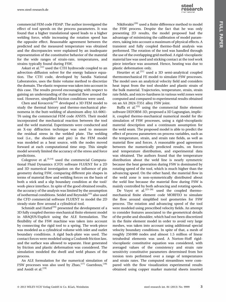
Figure 4b–d shows the evolution of the pressure

computed by the two models at three reference points

defined in Figure 4a. Points 1 and 2 move with the mesh,


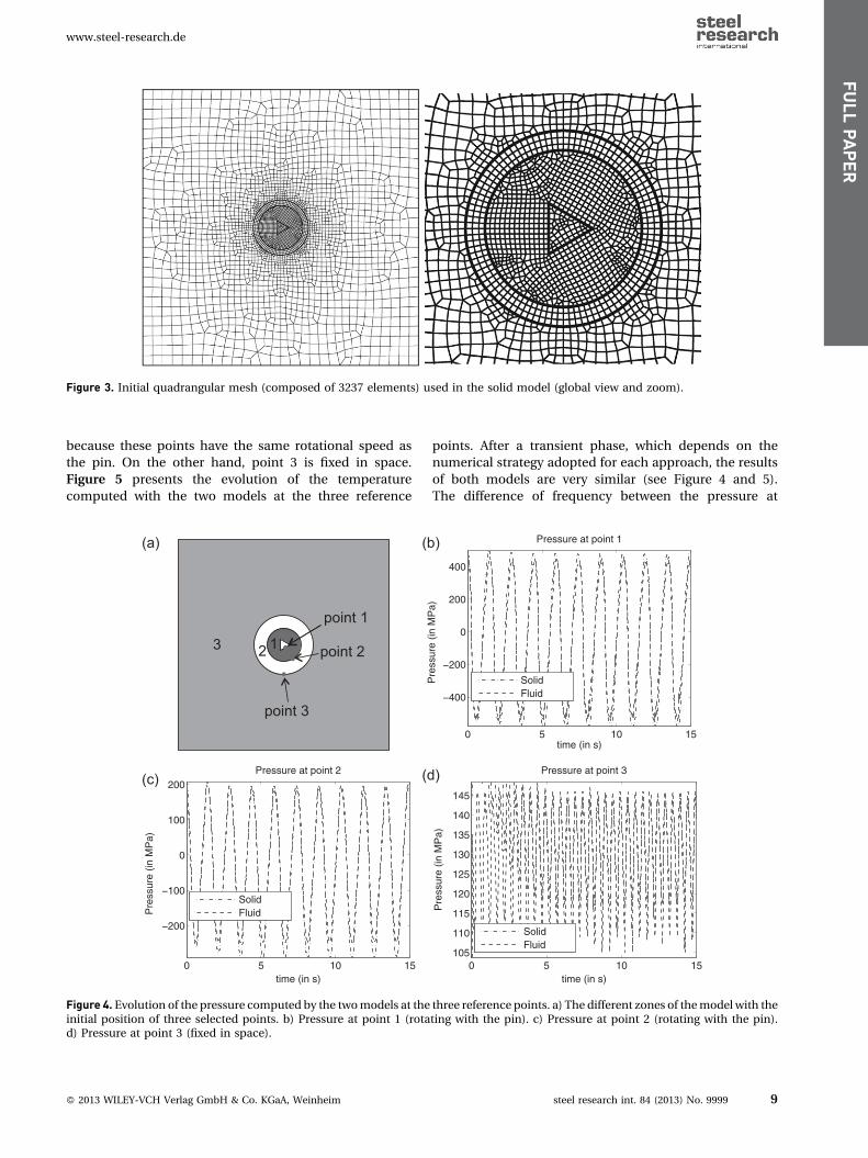
Figure 3. Initial quadrangular mesh (composed of 3237 elements) used in the solid model (global view and zoom).


FULL

PAPER

because these points have the same rotational speed as

the pin. On the other hand, point 3 is fixed in space.

Figure 5 presents the evolution of the temperature

computed with the two models at the three reference

3 2 1

point 1

point 2

point 3

0 5 10 15

−200

−100

0

100

200

time (in s)

Pre

ssur

e (in

MP

a)

Pressure at point 2

SolidFluid

(a)

(c)

(b

(d

Figure 4. Evolution of the pressure computed by the twomodels at theinitial position of three selected points. b) Pressure at point 1 (rotad) Pressure at point 3 (fixed in space).


points. After a transient phase, which depends on the

numerical strategy adopted for each approach, the results

of both models are very similar (see Figure 4 and 5).

The difference of frequency between the pressure at

0 5 10 15

−400

−200

0

200

400

time (in s)

Pre

ssur

e (in

MP

a)

Pressure at point 1

SolidFluid

0 5 10 15105

110

115

120

125

130

135

140

145

time (in s)

Pre

ssur

e (in

MP

a)

Pressure at point 3

SolidFluid

)

)

three reference points. a) The different zones of themodel with theting with the pin). c) Pressure at point 2 (rotating with the pin).


0 5 10 1520

40

60

80

100

120

140

time (in s)

Tem

pera

ture

(in

°C

elsi

us)

Temperature at point 1

SolidFluid

0 5 10 1520

30

40

50

60

70

80

90

100

110

time (in s)

Tem

pera

ture

(in

°C

elsi

us)


SolidFluid

0 5 10 1520

30

40

50

60

70

80

90

100

time (in s)

Tem

pera

ture

(in

°C

elsi

us)


SolidFluid

(a)

(b) (c)

Figure 5. Evolution of the temperature computed by the twomodels at the three reference points. a) Temperature at point 1 (rotatingwiththe pin). b) Temperature at point 2 (rotating with the pin). c) Temperature at point 3 (fixed in space).


FULL

PAPER

point 3 and the pressure and the temperature at points 1

and 2 is explained by the fact that point 3 is fixed in space

while points 1 and 2 have the same rotational velocity as

the pin. On the one hand, the pressure at point 3 is affected

by the three corners of the pin. On the other hand, the

frequency of the pressure and the temperature at points 1

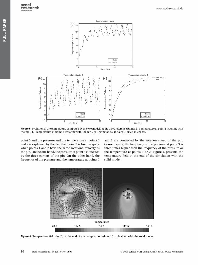
Figure 6. Temperature field (in 8C) at the end of the computation (t


and 2 are controlled by the rotation speed of the pin.

Consequently, the frequency of the pressure at point 3 is

three times higher than the frequency of the pressure or

the temperature at points 1 or 2. Figure 6 presents the

temperature field at the end of the simulation with the

solid model.

ime: 15 s) obtained with the solid model.



FULL

PAPER

4. Conclusion and Future Works

The phenomena happening during the FSW process are

at the interface between solid mechanics and fluid

mechanics. In this paper, two different methods are

presented to simulate the FSW process numerically. One

model is based on a solid approach which computes the

position and the temperature fields and another one is

based on a fluid approach written in terms of velocity,

pressure, and temperature fields. Both models use

advanced numerical techniques such as the ALE formal-

ism or remeshing operations or an advanced stabilization

algorithm. These advanced numerical techniques allow

the simulation of the FSW process with non-circular tool

shapes. The aim of the paper was to compare two

computational models based respectively on solid and

fluid approach for the solution of FSW process. Based on

the authors’ point of view, being able to simulate a

process using a solid model and at the same time a fluid

model, is numerically very interesting and represents a

further verification of the implementation in both

approaches. The presented example (with a triangular

pin) shows that the two formulations essentially deliver

the same results. More investigations are still needed to

understand the small differences between the two

models. While the fluid model is more efficient from a

computational point of view, the model based on the

solid approach has the advantage that it can be

used to compute the residual stresses (the thermo-

visco-plastic constitutive model can be replaced with a

thermo-elasto-visco-plastic one).

Acknowledgment

The Belgian authors wish to acknowledge the Walloon

Region for its financial support to the STIRHETAL project

(WINNOMAT program, convention number 0716690) in

the context of which this work was performed.

Revised: May 6, 2013;

Keywords: Arbitrary Lagrangian–Eulerian (ALE)

formalism; finite element method; friction stir welding

(FSW); remeshing

References

[1] W. M. Thomas, E. D. Nicholas, J. C. Needham,

M. G. Murch, P. Temple-Smith, C. J. Dawes, GB

Patent No. 9125978.8, International Patent No.

PCT/GB92/02203, 1991.

[2] J. C. McClure, W. Tang, L. E. Murr, X. Guo, Z. Feng,

J. E. Gould, in Proc. of the 5th Int. Conf. on Trends in

Welding Research, Pine Mountain, Georgia, USA,

June 1–5, 1998, pp. 590.


[3] P. Colegrove, M. Painter, D. Graham, T. Miller, in

Proc. of the 2nd Int. Symp. on Friction Stir Welding

(2ISFSW), Gothenburg, Sweden, June 27–29, 2000.

[4] M. Khandkar, J. Khan, J. Mater. Process. Manuf. Sci.

2001, 10, 91. DOI: 10.1177/1062065602010002613

[5] M. Khandkar, J. Khan, A. Reynolds, Sci. Technol. Weld.

Join. 2003, 8(3), 165. DOI: 10.1179/

136217103225010943

[6] G. Bendzsak, T. North, C. Smith, An experimentally

validated 3D model for friction stir welding, in Proc.

of the 2nd Int. Symp. on Friction Stir Welding

(2ISFSW), Gothenburg, Sweden, June 27–29, 2000.

[7] G. Bendzsak, T. North, C. Smith, Material properties

relevant to 3-D fsw modeling, in Proc. of the 2nd Int.

Symp. on Friction Stir Welding (2ISFSW),

Gothenburg, Sweden, June 27–29, 2000.

[8] P. Dong, F. Lu, J. K. Hong, Z. Cao, Sci. Technol. Weld.

Join. 2001, 6(5), 281. DOI: 10.1179/

136217101101538884

[9] S. Xu, X. Deng, A. P. Reynolds, T. U. Seidel, Sci.

Technol. Weld. Join. 2001, 6(3), 191. DOI: 10.1179/

136217101101538640

[10] S. Xu, X. Deng, In Proc. of the 4th Int. Symp. on

Friction Stir Welding (4ISFSW), Park City, Utah, USA,

May 14–16, 2003.

[11] P. Ulysse, Int. J. Mach. Tools Manuf. 2002, 42, 1549.

DOI: 10.1016/S0890-6955(02)00114-1

[12] A. Askari, S. Silling, B. London, M. Mahoney, in Proc.

of the 4th Int. Symp. on Friction Stir Welding

(4ISFSW), GKSS Workshop, Park City, Utah, USA,

May 14–16, 2003.

[13] C. M. Chen, R. Kovacevic, Int. J. Mach. Tools Manuf.

2003, 43(13), 1319. DOI: 10.1016/S0890-6955(03)

00158-5

[14] P. Colegrove, H. Shercliff, P. Threadgill, in Proc. of the

5th Int. Symp. on Friction Stir Welding (5ISFSW),

Metz, France, September 14–16, 2004.

[15] T. U. Seidel, A. P. Reynolds, Sci. Technol. Weld. Join.

2003, 8(3), 175. DOI: 10.1179/136217103225010952

[16] H. Schmidt, J. Hattel, In Proc. of the 5th Int. Symp. on

Friction Stir Welding (5ISFSW), Metz, France,

September 14–16, 2004.

[17] H. Zhao, PhD thesis, West Virginia University

(Morgantown, West Virginia, USA) 2005. URL http://

hdl.handle.net/10450/4367

[18] S. Guerdoux, PhD thesis, Ecole Nationale Superieure

des Mines de Paris, 2007.

[19] M. Assidi, L. Fourment, S. Guerdoux, T. Nelson, Int. J.

Mach. Tools Manuf. 2010, 50(2), 143. DOI: 10.1016/j.

ijmachtools.2009.11.008

[20] N. Nikiforakis, in Proc. of the 2nd FSW Modelling and

Flow Visualisation Seminar, GKSS

Forschungszentrum, Geesthacht, Germany,

January 31–February 1, 2005.

[21] P. Heurtier, M. J. Jones, C. Desrayaud, J. H. Driver,

F. Montheillet, D. Allehaux, J. Mater. Process. Technol.


http://hdl.handle.net/10450/4367



FULL

PAPER
2006, 171(3), 348. DOI: 10.1016/j.
jmatprotec.2005.07.014

[22] G. Buffa, J. Hua, R. Shivpuri, L. Fratini, Mater. Sci.

Eng. A 2006, 419(1–2), 389. DOI: 10.1016/j.

msea.2005.09.040

[23] T. De Vuyst, L. D’Alvise, A. Simar, B. de Meester,

S. Pierret, Weld. World 2005, 49(3/4), 44.

[24] T. De Vuyst, L. D’Alvise, A. Simar, B. de Meester,

S. Pierret, in Proc. of the 5th Int. Symp. on Friction Stir

Welding (5ISFSW), Metz, France, September 14–16,

2004.

[25] T. De Vuyst, L. D’Alvise, A. Robineau, J. C. Goussain,

in Proc. of the 8th Int. Seminar on Numerical Analysis

of Weldability, Graz, Austria, September 25–27,

2006.

[26] T. De Vuyst, L. D’Alvise, A. Robineau, J. C. Goussain,

in Proc. of the 6th Int. Symp. on Friction Stir Welding

(6ISFSW), Saint-Sauveur, Quebec, Canada,

October 10–13, 2006.

[27] H. R. Shercliff, M. J. Russell, A. Taylor, T. L. Dickerson,

Mec. Ind. 2005, 6(1), 25. DOI: 10.1051/meca:2005004

[28] R. Lopez, B. Ducoeur, M. Chiumenti, B. de Meester,

C. Agelet de Saracibar, Int. J. Mater. Form. 2008, 1,

1291. DOI: 10.1007/s12289-008-0139-4

[29] C. Agelet de Saracibar, R. Lopez, B. Ducoeur,

M. Chiumenti, B. de Meester, Rev. Int. Metodos

Numericos para Calculo y Diseno en la Ingenierıa

2013, 29, 29. DOI: 10.1016/j.rimni.2012.02.003

[30] D. Santiago, G. Lombera, S. Urquiza, C. Agelet de

Saracibar, M. Chiumenti, Rev. Int. Metodos Numericos

para Calculo y Diseno en Ingenierıa 2010, 26, 293.

[31] C. Agelet de Saracibar, M. Chiumenti, D. Santiago,

N. Dialami, G. Lombera, in Proc. of the Int. Symp. on

Plasticity and its Current Applications, Plasticity, St.

Kitts, St. Kitts and Nevis, January 3–8, 2010.

[32] C. Agelet de Saracibar, M. Chiumenti, D. Santiago,

M. Cervera, N. Dialami, G. Lombera, in Proc. of the

10th Int. Conf. on Numerical Methods in Industrial

Forming Processes, Volume 1252, Pohang, South

Korea, June 13–17 2010, AIP Conf. Proc., pp. 81–88.

DOI: 10.1063/1.3457640

[33] C. Agelet de Saracibar, M. Chiumenti, M. Cervera,

N. Dialami, D. Santiago, G. Lombera, in Proc. of the

Int. Symp. on Plasticity and its Current Applications,

Plasticity, Puerto Vallarta, Mexico, January 3–8, 2011.

[34] M. Chiumenti, M. Cervera, C. Agelet de Saracibar,

N. Dialami, Comput. Methods Appl. Mech. Eng. 2013,

254, 353. DOI: 10.1016/j.cma.2012.09.013


[35] N. Dialami, M. Chiumenti, M. Cervera, C. Agelet de

Saracibar, Comput. Struct. 2013, 117, 48. DOI:

10.1016/j.compstruc.2012.12.006

[36] M. Chiumenti, M. Cervera, C. Agelet de Saracibar,

N. Dialami, NUMIFORM 2013, 11th International

Conference on Numerical Methods in Industrial

Forming Processes, Shenyang, Liaoning, China, 6–10

July 2013, AIP Conference Proceedings, 1532, 45

(2013).

[37] M. Cervera, C. Agelet de Saracibar, M. Chiumenti,

Comet – A Coupled Mechanical and Thermal Analysis

Code. Data Input Manual. Version 5.0. Technical

Report IT-308, CIMNE, Barcelona, Spain, 2002. URL

http://www.cimne.com/comet

[38] C. Agelet de Saracibar, M. Chiumenti, Q. Valverde,

M. Cervera, Comput. Methods Appl. Mech. Eng. 2006,

195, 1224. DOI: 10.1016/j.cma.2005.04.007

[39] M. Cervera, M. Chiumenti, Q. Valverde, C. Agelet de

Saracibar, Comput. Methods Appl. Mech. Eng. 2003,

192, 5249.

[40] M. Chiumenti, Q. Valverde, C. Agelet de Saracibar,

M. Cervera, Int. J. Plast. 2004, 20, 1487. DOI: 10.1016/

j.ijplas.2003.11.009

[41] C. Agelet de Saracibar, M. Cervera, M. Chiumenti,

Int. J. Plast. 1999, 15, 1.

[42] M. Cervera, C. Agelet de Saracibar, M. Chiumenti,

Int. J. Numer. Methods Eng. 1999, 46, 1575–1591.

[43] J. Donea, A. Huerta, J.-P. Ponthot, A. Rodrıguez-

Ferran, Encyclopedia of Computational Mechanics,

John Wiley & Sons, Ltd, 2004. DOI: 10.1002/

0470091355.ecm009

[44] R. Boman, J.-P. Ponthot, Int. J. Numer. Methods Eng.

2012, 92, 857. DOI: 10.1002/nme.4361

[45] R. Boman, J.-P. Ponthot, Int. J. Impact Eng. 2013, 53,

62. DOI: 10.1016/j.ijimpeng.2012.08.007

[46] P. Bussetta, R. Boman, J.-P. Ponthot, Novel three-

dimensional data transfer operators using auxiliary

finite volume mesh or mortar elements and based over

numerical integration, in preparation.

[47] P. Bussetta, J.-P. Ponthot, in Proc. of the 18th Int.

Symp. on Plasticity and Its Current Applications, San

Juan, Puerto Rico, January, 2012. URL http://hdl.

handle.net/2268/100394

[48] J. P. Ponthot, Int. J. Plast. 2002, 18, 91. DOI: 10.1016/

S0749-6419(00)00097-8

[49] C. Agelet de Saracibar, M. Chiumenti, M. Cervera,

N. Dialami, A. Seret, Arch. Comput. Methods Eng.

2014, accepted for publication.


http://www.cimne.com/comet



Documents

Comparison of a Fluid and a Solid Approach for the ...cervera.rmee.upc.edu/papers/2014-SRI-comparison-no.pdf · Comparison of a Fluid and a Solid Approach for the Numerical Simulation