ITEMS instructional Topics in Educational Measurement

An NCME Instructional Module on

Comparison of 11, 20, and 31Parameter IRT Models Deborah Harris American College Testing Program

This module discusses the I - , 8-, and 8-parameter logistic item re- sponse theory models. Mathematical formulas are given fm eaeh model, and comparisons among the three models are made. Figures are in- cluded to illustrate the effects of changing the a, b, or c parameter, and a single data set is used to illustrate th.e effects of estimating parameter values (as opposed to the true parameter values) and to compare parameter estimates achieved though applying the different models. The estimation procedure itself is discussed briefly. Discus- sions ofmodel assumptions, such as dimensionality and local in&- pendace, can be f&nd in many of the annotated rejermes (e.g., Hambleton, 1988).

Item response theory (IRT) attempts to model the relation- ship between an unobserved variable, usually conceptualized as an examinee’s ability, and the probability of the examinee correctly responding to any particular test item. Three cur- rently used models are the 3-parameter logistic, the 2-para- meter logistic, and the 1-parameter logistic models. (The 1-parameter model is referred to as the Rasch model.) These models all assume a single underlying ability-usually a con- tinuous, unbounded variable designated as &for examinees, but vary in the characteristics they ascribe to items. All three models have an item difficulty parameter (b), which is the

Deborah Harris is a P s y c h t r i c b n , American College Testing Program, P.O. Box 168, Iowa City, IA 52249. She specializes in

Series I n f m t i o n ITEMS is a series of units designed to facilitate instruction in

educational measurement. These units are published by the Na- tional Council on Measurement in Education. This module may be photocopied without permission if reproduced in its entirety and used for instructional purposes. Fred Brown, Iowa State University, has served as the editor for this module.

psychometrics.

point of inflection on the ability (6) scale. For the 1-parameter and 2-parameter models, this is the point on the ability (0) scale at which an examinee has a 50% probability of correctly answering an item. For the 3-parameter item, this is the point at which the probability of correctly answering an item is (1 + c)/2, where c is a lower asymptote parameter (see the discussion that follows). Theoretically, difficulty values can range from - 00 to + 00; in practice, values usually are in the range of - 3 to + 3, when 0 is scaled to have a mean of 0 and standard deviation of 1.0. Similarly, examinee ability values can range from - 00 to + 00, but values in excess of * 3 seldom are seen. Items with high values of b are hard items, with low-ability examinees having low probabilities of correctly responding to the item. Items with low values of b are easy items, with most examinees, even those with low-ability values, having a t least a moderate probability of answering the item correctly.

The 3- and 2-parameter models also have a discrimination parameter (a) that allows items to differentially discriminate among examinees. Technically, a is defined as the slope of the item characteristic curve (ICC) at the point of inflection (see Baker, 1985, p. 21). The a parameter can range in value from - QD to + 00, with typical values being d 2.0 for multiple- choice items. The higher the a value, the more sharply the item discriminates between examinees at the point of inflection.

The 3-parameter model also has a lower asymptote para- meter (c), which is sometimes referred to as the pseudochance parameter. This parameter allows for examinees, even ones with low ability, to have perhaps substantial probability of correctly answering even moderate or hard items. Theoretically, c ranges from 0.0 to 1.0, but is typically < 0.3.

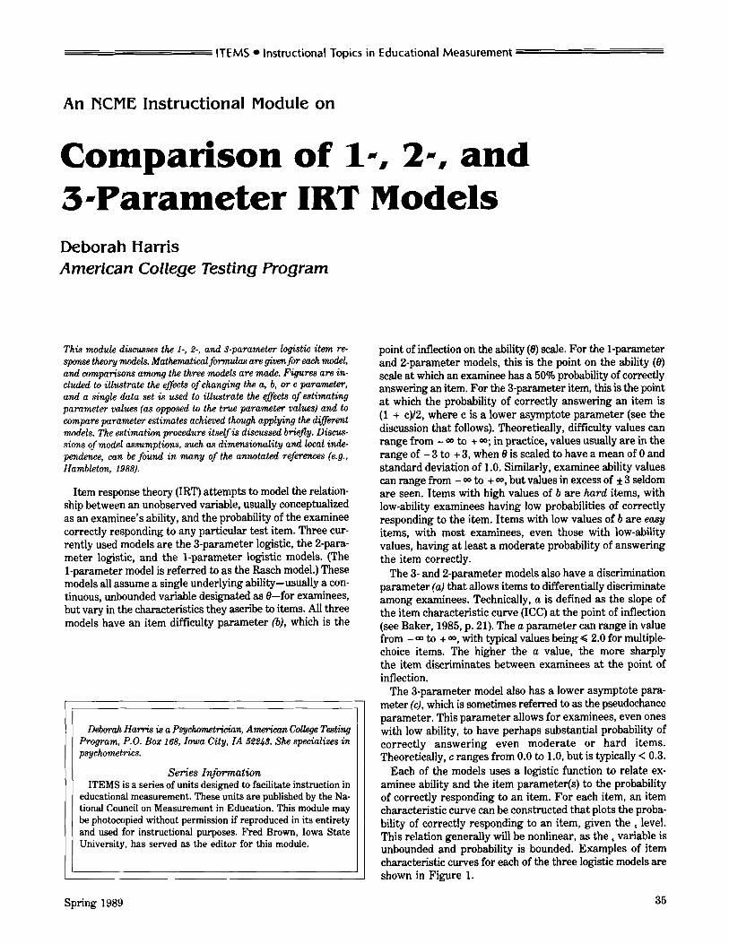
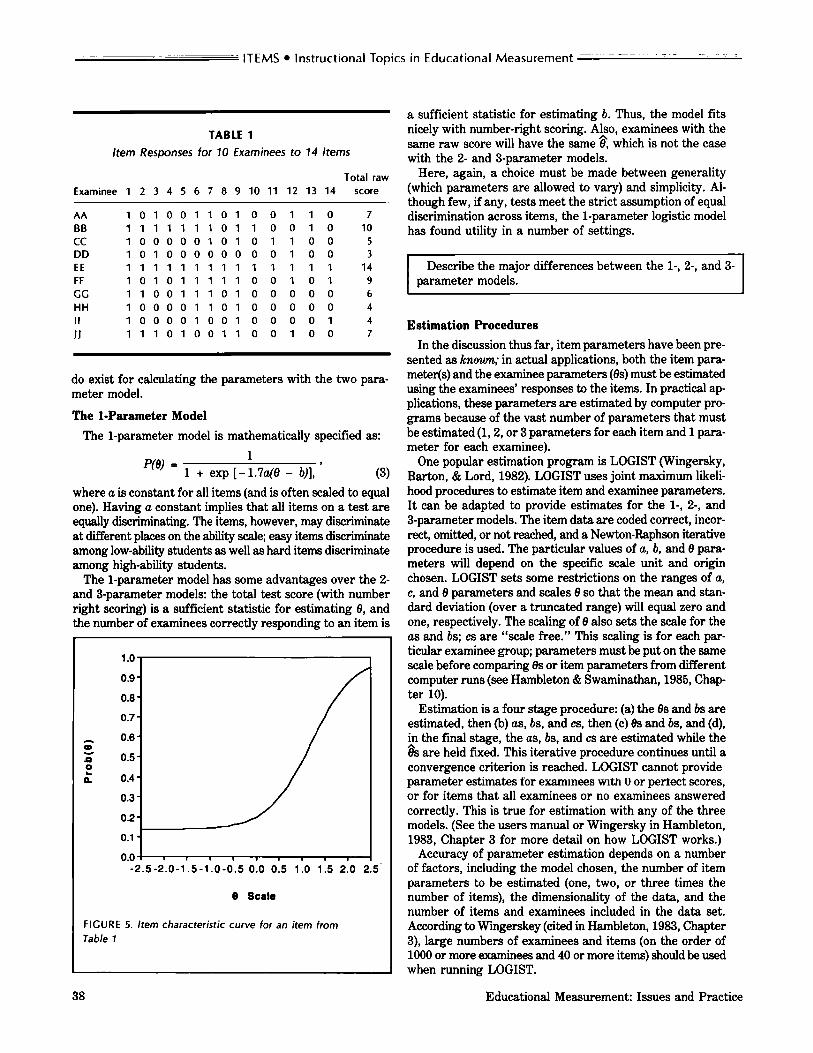
Each of the models uses a logistic function to relate ex- aminee ability and the item parameter@) to the probability of correctly responding to an item. For each item, an item characteristic curve can be constructed that plots the proba- bility of correctly responding to an item, given the level. This relation generally will be nonlinear, as the variable is unbounded and probability is bounded. Examples of item characteristic curves for each of the three logistic models are shown in Figure 1.

35 Spring 1989

ITEMS Instructional Topics in Educational Measurement

1.01 I

-2.5-2.0-1.5-1.0-0.5 0.0 0.5 1.0 1.5 2.0 2.5

e Scale

Iparameter logistic model

0.9

-2.5-2.0-1.5-1.0-0.5 0.0 0.5 1.0 1.5 2.0 2.5

e Scale (b) 2-parameter logistic model

c a

P 0 b

-2.5-2.0-1.5-1.0-0.5 0.0 0.5 1.0 1.5 2.0 2.5

e Scale (c) 7-parameter logistic model

FIGURE 1. Examples of item characteristic curves derived from the 3-, 2- and 'I-parameter logistic models

Define the three parameters used to describe items in the 1-, 2-, and 3-parameter models.

The 3-Parameter Model The 3-parameter model is defined mathematically as:

(1 - c) , (1)

p(e) = c + 1 + exp [-1.7a(8 - b)]

where a, b, and c are as defined above. The effects of varying different parameters in a 3-para-

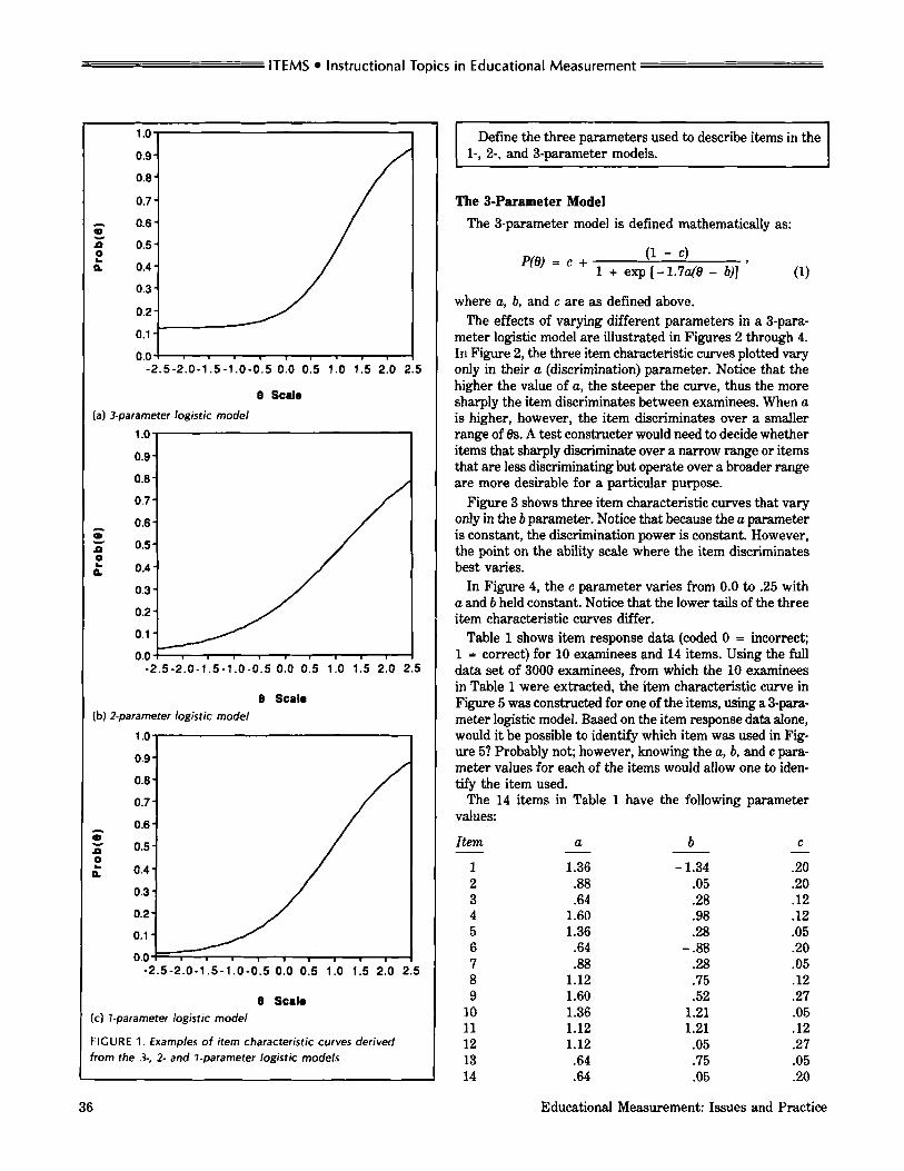
meter logistic model are illustrated in Figures 2 through 4. In Figure 2, the three item characteristic curves plotted vary only in their a (discrimination) parameter. Notice that the higher the value of a, the steeper the curve, thus the more sharply the item discriminates between examinees. When a is higher, however, the item discriminates over a smaller range of 0s. A test constructer would need to decide whether items that sharply discriminate over a narrow range or items that are less discriminating but operate over a broader range are more desirable for a particular purpose.

Figure 3 shows three item characteristic curves that vary only in the b parameter. Notice that because the a parameter is constant, the discrimination power is constant. However, the point on the ability scale where the item discriminates best varies.

In Figure 4, the c parameter varies from 0.0 to .25 with a and b held constant. Notice that the lower tails of the three item characteristic curves differ.

Table 1 shows item response data (coded 0 = incorrect; 1 = correct) for 10 examinees and 14 items. Using the full data set of 3000 examinees, from which the 10 examinees in Table 1 were extracted, the item characteristic curve in Figure 5 was constructed for one of the items, using a 3-para- meter logistic model. Based on the item response data alone, would it be possible to identify which item was used in Fig- ure 5? Probably not; however, knowing the a, b. and c para- meter values for each of the items would allow one to iden- tlfy the item used.

The 14 items in Table 1 have the following parameter values:

Item

1 2 3 4 5 6 7 8 9

10 11 12 13 14

- a

1.36 .88 .64

1.60 1.36 .64 .88

1.12 1.60 1.36 1.12 1.12 .64 .64

b

- 1.34 .05 .28 .98 .28

- .88 .28 .75 .52

1.21 1.21 .05 -75 .05

C

.20

.20

.12 -12 .05 .20 -05 .12 .27 .05 .12 .27 .05 .20

36 Educational Measurement: Issues and Practice

~~ -~ ~~~

-- ITEMS Instructional Topics in Educational Measurement ~~~~~ ~- ~~ ~~

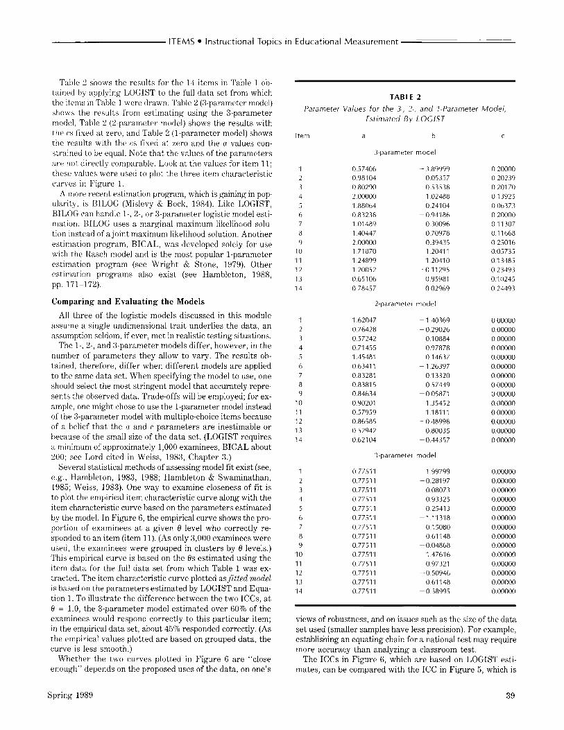
Using this information, t ry to determine what item’s char- acteristic curve is plotted in Figure 5.

Noting that the point of inflection (b) is slightly greater than + 1 .00, that the lower asymptote (c) is slightly above . lo, and that the slope at the point of inflection is ra ther steep, one could deduce that item 11 is the one plotted. The item char- acteristic curve was constructed by inserting the given para- meter values into Equation 1 for various 8 values. To illu- s t ra te , for 8 = 1.0:

(1.00 - . la) P(l.O) = . I2 + = ,47319,

1.00 + exp [ - 1.7(1.12)(1.00 - 1.2l)l which is the value plotted against 8 = 1.0 in Figure 5. Similar calculations were done for other values of 8.

The item characteristic curve shows the probability of re- sponding correctly to a n item for any given 8 level. F o r item 11, the probability of a n examinee with 8 = 1.0 correctly responding is .47. This means that (a) on average, in a group of 100 examinees with 8s equal to 1.0, 47 will correctly re- spond to item 11, o r (b) a given examinee with 8 = 1.0, when presented with 100 items similar to item 11, will answer cor- rectly, on average, 47% of the items.

The 10 examinees used in Table 1 have 8 values of - .05, 3 5 , -.45, -1.50, 1.95, .51, .64, -.57, -.21, and -.47, respec- tively. Note that although examinee CC has a higher 8 than examinee JJ, examinee JJ had a higher raw score. Although the 8 level indicates the “amount of ability” a n examinee has, it does not “predict” the examinee’s test score without er- ror. To illustrate how this can be, consider the probabilities of correctly answering a given item. The probability of a n examinee with a 8 of -.47 answering item 3 correctly is ,38779; the probability of a n examinee with a 8 of - .45 cor- rectly answering item 3 is 39186, and the probability of a n examinee with a 8 of .64 correctly answering item 3 is .64278. In this data set, however, examinee JJ (with a 8 of - .47) responded correctly to itern 3 whereas examinee CC (8 =

- .45) and examinee GG (8 = .64) responded incorrectly. The data set in Table 1 was generated using known 8 values. Results can be more anomalous when estimated ability values (8s) are used instead of 8s.

The 2-Parameter Model The %parameter logistic model is mathematically specified

as:

1 1 + exp [-1.7@ - b)] (2)

Note tha t if c was set equal to zero in Equation 1, Equation 2 would result. Setting the c parameter to zero implies that a n examinee of sufficiently low ability could have near zero probability of correctly responding to a n item, which might be the case with supply rather than selection items.

Although the %parameter model is less general than the 3-parameter, in that it does not allow the lower asymptote to vary, the 2-parameter model sometimes is preferred be- cause of the difficulties in estimating the c parameter in real data sets. Unlike the 3-parameter model, sufficient statistics

Spring 1989

p(e) =

0.9- ........................ &I B=O C=O I 1

0.7 -

0.6 - 0.5 - 0.4 -

- 2 . 5 - 2 . 0 - 1 . 5 - 1 . 0 - 0 . 5 0.0 0.5 1.0 1.5 2.0 2.5

fJ Scale

FIGURE 2 lCC5 derived by varying the a parameter in a 3-parameter logistic model

0.9 _ .................... A=

0.8 - - - - - - - - - A=l.B=l,C=O

I I I I I

- 2 . 5 - 2 . 0 - 1 . 5 - 1 . 0 - 0 . 5 0.0 0.5 1.0 1.5 2.0 2.5

0 Scale FIGURE 3 lCCs derived by varying the b parameter in a 3-parameter logistic model

-2 .5 -2 .0 -1 .5 -1 .0 -0 .5 0.0 0.5 1.0 1.5 2.0 2.5

0 Scale

FIGURE 4. lCCs derived by varying the c parameter in a 3-parameter logistic model

37

ITEMS Instructional Topics in Educational Measurement ~

~ -~ ~- ~~

0.9 - 0.8 - 0.7 - - 0.6-

c 2 p 0.5-

a 0.4-

0.3 -

TABLE 1 ltem Responses for 70 Examinees to 74 Items

Total raw Examinee 1 2 3 4 5 6 7 8 9 10 11 12 13 14 score

AA 1 0 1 0 0 1 1 0 1 0 0 1 1 0 7 BB 1 1 1 1 1 1 1 0 1 1 0 0 1 0 10 cc 1 0 0 0 0 0 1 0 1 0 1 1 0 0 5 DD 1 0 1 0 0 0 0 0 0 0 0 1 0 0 3 EE 1 1 1 1 1 1 1 1 1 1 1 1 1 1 14 FF 1 0 1 0 1 1 1 1 1 0 0 1 0 1 9 GG 1 1 0 0 1 1 1 0 1 0 0 0 0 0 6 HH 1 0 0 0 0 1 1 0 1 0 0 0 0 0 4 II 1 0 0 0 0 1 0 0 1 0 0 0 0 1 4 J J 1 1 1 0 1 0 0 1 1 0 0 1 0 0 7

do exist for calculating the parameters with the two para- meter model.

The 1-Parameter Model The 1-parameter model is mathematically specified as:

1 1 + exp [-1.7a(e - b)],

, (3)

where a is constant for all items (and is often scaled to equal one). Having a constant implies that all items on a test are equally discriminating. The items, however, may discriminate at different places on the ability scale; easy items d i ~ c r i m i ~ t e among low-ability students as well as hard items discriminate among high-ability students.

The 1-parameter model has some advantages over the 2- and 3-parameter models: the total test score (with number right scoring) is a sufficient statistic for estimating 0, and the number of examinees correctly responding to an item is

p(e) =

1 1 I 1.07 r I

:::I-’, , , , 1 0.0

-2.5-2.0-1.5-1.0-0.5 0.0 0.5 1.0 1.5 2.0 2.5

I e Scale

FIGURE 5. ltem characteristic curve for an item from Table 1

a sufficient statistic for estimating b. Thus, the model fits nicely with number-right scoring. Ako, examinees with the same raw score will have the same 8, which is not the case with the 2- and 3-parameter models.

Here, again, a choice must be made between generality (which parameters are allowed to vary) and simplicity. Al- though few, if any, tests meet the strict assumption of equal discrimination across items, the 1-parameter logistic model has found utility in a number of settings.

Describe the major differences between the 1-, 2-, and 3- parameter models.

Estimation Procedures In the discussion thus far, item parameters have been pre-

sented as Imown; in actual applications, both the item para- meter(s) and the examinee parameters (&) must be estimated using the examinees’ responses to the items. In practical ap- plications, these parameters are estimated by computer pro- grams because of the vast number of parameters that must be estimated (1,2, or 3 parameters for each item and 1 para- meter for each examinee).

One popular estimation program is LOGIST (Wingersky, Barton, & Lord, 1982). LOGIST uses joint maximum likeli- hood procedures to estimate item and examinee parameters. It can be adapted to provide estimates for the 1-, 2-, and 3-parameter models. The item data are coded correct, incor- rect, omitted, or not reached, and a Newton-Raphson iterative procedure is used. The particular values of a, b, and 0 para- meters will depend on the specific scale unit and origin chosen. LOGIST sets some restrictions on the ranges of a, c, and 8 parameters and scales 8 so that the mean and stan- dard deviation (over a truncated range) will equal zero and one, respectively. The scaling of 8 also sets the scale for the as and bs; cs are “scale free.” This scaling is for each par- ticular examinee group; parameters must be put on the same scale before comparing 8s or item parameters from different computer runs (see Hambleton & Swaminathan, 1985, Chap- ter 10).

Estimation is a four stage procedure: (a) the 8s and bs are estimated, then (b) as, bs, and cs, then (c) 8s and bs, and (d), in the final stage, the as, bs, and cs are estimated while the 0s are held fixed. This iterative procedure continues until a convergence criterion is reached. LOGIST cannot provide parameter estimates for examinees unth 0 or pellect scores, or for items that all examinees or no examinees answered correctly. This is true for estimation with any of the three models. (See the users manual or Wingersky in Hambleton, 1983, Chapter 3 for more detail on how LOGIST works.)

Accuracy of parameter estimation depends on a number of factors, including the model chosen, the number of item parameters to be estimated (one, two, or three times the number of items), the dimensionality of the data, and the number of items and examinees included in the data set. According to Wingerskey (cited in Hambleton, 1983, Chapter 3), large numbers of examinees and items (on the order of 1000 or more examinees and 40 or more items) should be used when running LOGIST.

h

Educational Measurement: Issues and Practice 38

_ _ _ _ ~ _____ ~_________ ~ ITEMS instructional Topics in Educational Measurement ~

~ ~- ~

Tahle 2 shows the results for the 14 items in Table 1 ob- tainrd by applying LOGIST to the full data set from which the items in Table 1 were drawn. Table 2 (3-parameter model) shows the results from estimating using the 3-parameter model, Table 2 (%parameter model) shows the results with the cs fixed at zero, and Table 2 (I-parameter model) shows the results with the cs fixed at zero and the a values con- strained to be equal. Note that the values of the parameters a re not directly comparable. Look at the values for item 11; these values were used to plot the three item characteristic curves in Figure 1

A more recent estimation program, which is gaining in pop- ularity, is BILOG (Mislevy & Bock, 1984). Like LOGIST, BILOG can handle 1-, 2-, o r 3-parameter logistic model esti- mation. HILOG uses a marginal maximum likelihood solu- tion instead of a joint maximum likelihood solution. Another estimation program, BICAL, was developed solely for use with the Rasch model and is the most popular 1-parameter estimation program (see Wright & Stone, 1979). Other estimation programs also exist (see Hambleton, 1988, pp. 171-172).

Comparing and Evaluating the Models All three of the logistic models discussed in this module

assume a single undimensional trait underlies the data , a n assumption seldom, if ever, met in realistic testing situations.

The 1-, 2-, and 3-parameter models differ, however, in the number of parameters they allow to vary. The results ob- tained, therefore, differ when different models are applied to the same data set. When specifying the model to use, one should select the most stringent model that accurately repre- sents the observed data. Trade-offs will be employed; for ex- ample, one might chose to use the 1-parameter model instead of the 5-parameter model with multiple-choice items because of a belief tha t the u and c parameters are inestimable or because of the small size of the data set. (LOGIST requires a minimum of approximately 1,000 examinees, BICAL about 200; see Lord cited in Weiss, 1983, Chapter 3.)

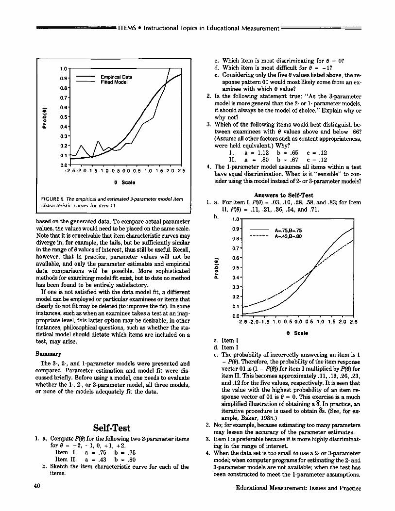
Several statistical methods of assessing model fit exist (see, e.g., Hambleton, 1983, 1988; Hambleton & Swaminathan, 1985; Weiss, 1983). One way t o examine closeness of fit is to plot the empirical item characteristic curve along with the item characteristic curve based on the parameters estimated by the model. In Figure 6, the empirical curve shows the pro- portion of examinees at a given 8 level who correctly re- sponded to an item (item 11). (As only 3,000 examinees were used, the examinees were grouped in clusters by 8 levels.) This empirical curve is ba.sed on the 8s estimated using the item data for the full data set from which Table 1 was ex- tracted. The item characteristic curve plotted asfitted model is based on the parameters estimated by LOGIST and Equa- tion l . To illustrate the difference between the two ICCs, at 8 = 1.0, the 3-parameter model estimated over 60% of the examinees would respond correctly to this particular item; in the empirical data set, about 459’0 responded correctly. (As the empirical values plotted are based on grouped data, the curve is less smooth.)

Whether the two curves plotted in Figure 6 are “close enough” depends on the proposed uses of the data, on one’s

TABLE 2

Parameter Values for the 3, 2-, and 7-Parameter Model,

Item

1 2 3 4 5 6 7 8 9

10 11 12 13 14

1 2 3 4 5 6 7 8 9

10 11 12 13 14

1 2 3 4 5 6 7 8 9

10 11 12 13 14

Estimated B y LOClST

a b

3-parameter model ~-

0 57406 0 981 04 0 80290 2 00000 188064 0 83238 1 01489 140447 2 00000 1 71870 124899 120052 0 651 06 0 78457

- 3 89999 0 05357 0 53538 102488 0 241 04

-094186 0 30096 0 70978 0 39435 1 20411 1 20410

-011295 0 95981 0 02969

2-parameter model

162047 0 76428 0 57242 0 71 455

0 63411 0 83281

0 84634 0 90201 0 57959

0 52942 0 62104

145481

0 8381 5

o 86585

- 1 40369 - 0 29026

0 10884

0 14637 -1 26397

0 13320 0 57449

- 0 05871 135452 118111

- 0 48998 0 80035

- 0 44357

0 97878

1-Dararneter model

0 77511 0 77511 0 77511 0 77511 0 77511 0 77511 0 77511 0 77511 0 77511 0 77511 0 7751 1 0 77511 0 7751 1 0 7751 1

-1 99799 -0 28197

0 08073 0 93325 0 2541 3

-1 11318 0 15080 061148

1 47616 0 97321

- 0 50946 061148

- 0 38995

- o 04868

C

0 20000 0 202 19 0 201 70 0 13925 0 06373 0 20000 011307 011668 0 25016 0 05735 0 13485 0 2 3493 0 10245 0 24493

0 00000 0 00000 0 00000 0 00000 0 00000 0 00000 0 00000 0 00000 0 00000 0 00000 0 00000 0 00000 0 00000 0 00000

0 00000 0 00000 0 00000 0 00000 0 00000 0 00000 0 00000 0 00000 0 00000 0 00000 0 00000 0 00000 0 00000 0 00000

views of robustness, and on issues such as the size of the data set used (smaller samples have less precision). F o r example, establishing a n equating chain for a national test may require more accuracy than analyzing a classroom test.

The ICCs in Figure 6, which a r e based on LOGIST esti- mates, can be compared with the ICC in Figure 5, which is

Spring 1989 39

ITEMS Instructional Topics in Educational Measurement

Empirical Data Fitted Model

0.9-

0.8 - 0.7 - 0.6 - 0.5 - 0.4 - 0.3 - 0.2 - 0.1 -

-

-2.5-2.0-1.5-1.0-0.5 0.0 0.5 1.0 1.5 2.0 2.5

0 Scale

FIGURE 6. The empirical and estimated Iparameter model item characteristic curves for item 17

based on the generated data. To compare actual parameter values, the values would need to be placed on the same scale. Note that it is conceivable that item characteristic curves may diverge in, for example, the tails, but be sufficiently similar in the range of 8 values of interest, thus still be useful. Recall, however, that in practice, parameter values will not be available, and only the parameter estimates and empirical data comparisons will be possible. More sophisticated methods for examining model fit exist, but to date no method has been found to be entirely satisfactory.

If one is not satisfied with the data model fit, a different model can be employed or particular examinees or items that clearly do not fit may be deleted (to improve the fit). In some instances, such as when an examinee takes a test at an inap- propriate level, this latter option may be desirable; in other instances, philosophical questions, such as whether the sta- tistical model should dictate which items are included on a test, may arise.

Summary The 3-, 2-, and 1-parameter models were presented and

compared. Parameter estimation and model fit were dis- cussed briefly. Before using a model, one needs to evaluate whether the 1-, 2-, or 3-parameter model, all three models, or none of the models adequately fit the data.

Self-Test 1. a. Compute P(8) for the following two 2-parameter items

for 8 = -2, -1, 0, +1, +2. Item I. a = .75 b = .75 Item 11. a = .43 b = .80

b. Sketch the item characteristic curve for each of the items.

c. Which item is most discriminating for 8 = O? d. Which item is most difficult for 8 = - l? e. Considering only the five 8 values listed above, the re-

sponse pattern 01 would most likely come from an ex- aminee with which 8 value?

2. Is the following statement true: “AS the 3-parameter model is more general than the 2- or 1- parameter models, it should always be the model of choice.” Explain why or why not?

3. Which of the following items would best distinguish be- tween examinees with 8 values above and below .66? (Assume all other factors such as content appropriateness, were held equivalent.) Why?

I . a = 1.12 b = .65 c = .12 11. a = $0 b = .67 c = .12

4. The 1-parameter model assumes all items within a test have equal discrimination. When is it “sensible” to con- sider using this model instead of 2- or 3-parameter models?

Answers to Self-Test 1. a. For item I, P(8) = .03, .lo, .28, .58, and 33; for Item

11, P(8) = .11, .21, .36, .54, and .71. b.

L5

c n z n

0.9- A-.75,B-.75 A-.43,B-.80

- ------ .

0.8 - 0.7 - 0.6 - 0.5 - 0.4 -

-2.5-2.0-1.5-1.0-0.5 0.0 0.5 1.0 1.5 2.0 2.5

8 Scale c. Item1 d. Item I e. The probability of incorrectly answering an item is 1

- P(8). Therefore, the probability of the item response vector 01 is (1 - P(8)) for item I multiplied by P(8) for item 11. This becomes approximately . 1 1, .19, .26, .23, and .12 for the five values, respectively. It is seen that the value with the highest probability of an item re- sponse vector of 01 is 8 = 0. This e5ercise is a much simplified illustration of obtaining a OA1n practice, an iterative procedure is used to obtain 8s. (See, for ex- ample, Baker, 1985.)

2. No; for example, because estimating too many parameters may lessen the accuracy of the parameter estimates.

3. Item I is preferable because it is more highly discriminat- ing in the range of interest.

4. When the data set is too small to use a 2- or 3-parameter model; when computer programs for estimating the 2- and 3-parameter models are not available; when the test has been constructed to meet the 1-parameter assumptions.

Educational Measurement: Issues and Practice 40

-. ITEMS Instructional Topics in Educational Measurement - - - - -

Annotated References Andrich, D. (1988). Rasch nlodeL9 for measurement. Beverly Hills,

CA: Sage. An introduction to Rasch modeling for social science measurement,

including a comparison with Guttman and Thurstone scaling. Raker, F. B. (1985). The basics ofitem response theory. Portsmouth,

NH: Heinemann Educational Books. Accompanied by an IBM or Apple disk. Covers models, estima-

tion. and fit; minimal math requirement; user friendly exercises, in- cluding graphing the item characteristic curves of 1-, 2-, and 3 para- meter models. A good hands-on introduction to IRT. Hambleton, R. K. (Ed.). (1983). Applications o f i t a response theory.

Vancouver: Educational Research Institute of British Columbia. Includes chapters on parameter estimation, choosing a model,

model-data fit, and LOGIST. Hamt)lehn, R. K., & Swaminathan. H. (1985). Item response t h e w :

Prin+ds and applieationu. Boston: Kluwer-Nijhoff. A good overview of IRT, requiring some mathematical background.

Includes chapters on estimating parameters and on model-data fit. Hambleton, R. K. (1988). Principles and selected applications of item

response theory. In R. L. Linn (Ed.) Edwtional mcapurement, (3rd ed., pp. 147-200). New York: Macmillan. Well-written introduction to IRT, including discussions of assump-

tions, different IRT models, testing model fit, and applications. Lord, F. M. (1980). Applicatiorw: of item reqmse ULegl to practical

testing y r o b l m ~ . Hillsdale, NJ: Erlbaum. Somewhat mathematical and theoretical, but readable. Discusses

item characteristic curves, models, and parameter estimation. Lord, F. M., & Novick, M. R. (1968). Statistical theories of mental

test scores. Reading, MA: Addison-Wesley. Chapters 16-20 present a mathematically sophisticated treatment

of IRT, including Allan Birnbaum’s introduction of logistic response models. Mislevy, R. J., & Bock, R. D. (1984). BILOG I (Version 2.2). Moores-

ville, IN: Scientific Software. Users manual for BILOG, a marginal maximum likelihood logistic

model estimation program. Warm, T. A. (1978). A p r i m e r of item response theory (Tech. Rep.

No. 941078). Oklahoma City, OK: U.S. Coast Guard Institute. An introductory text that utilizes a nonmathematical approach to

the fundamentals of IRT; quite readable for a novice. Weiss. D. J. (Ed.). (1983). New horizons in testing: Latent trait theiry

und computerized adaptive testing. New York: Academic Press. Sections on parameter estimating, including robustness and person-

to-model fit. Mathematical demands vary. Wingersky, M. S.. Barton, M. A., & Lord. F. M. (1982). LOGIST

5 (Version 1.0). Princeton, NJ: Educational Testing Service. A joint maximum likelihood logistic model estimation program.

Wright, B. I).. & Stone, M. H. (1979). Best test design. R d masure- mcmt. Chicago, I L MESA. Concentrates on the Rasch model; includes example of item calibra-

tion by hand, model fit, and discussion of BICAL.

Teaching Aids Are Available A set of teaching aids, designed by Deborah Harris

to complement her ITEMS module, “Comparison of 1-, 2-, and 3-Parameter IRT Models,” is available at cost from NCME. These teaching aids contain a set of item responses for 200 people to 14 items, along with the a, b, and c parameters and the 8 values. As long as they are available, they can be obtained by sending $2.00 to: Teaching Aids, ITEMS Module #7, NCME, 1230 17th St., NW, Washington, DC 20036.

Spring 1989

Instructional Topics in Educational

Measurement Series (ITEMS)

About ITEMS The purpose of tho 1nstructioii;il Topics in Kducational Me;i-

xurcwient Scrics (ITEMS) is to improve the iii~lershndirig 1 I f etlucational measurement principles. These materials are designed for use hy college fiiculty and students as well a s 1)y workshop Icatlcrs and p;wticipants.

This series is the outcome of ;in NCME ‘l‘ask Force estah- lished i n 19x6 in response to ii pcweived need for materials I O improve t.he communication ;itid undcrskinding of educa- t.ional mciisurc‘ment principles. The comniitt.ee is chaired hy Al Oosterhof, Florida Stah Ilniversity. Other nieml)ers of the commit.tee arc Fred Rrown. 1ow;i State Ilniversity; ,Jason Mil lman. Cornell University; iintl Ikirlxira S. Plake. IJniver- sity of Nebraska.

‘I‘opics for the series were itientificd from the results of a survey of R ranrloni simple of NCMK memtwrs. Authors were selected from persons either responding to a call for authors h a t appeared in Ed/:tl,c.vtr/ iotrtrl M(ifI.s/i.t,(itt~(~i/: Is.s/u?s r r / d Pwc- / iw or through individual contxts by the committee mem- bers. Currently, 17 authors arc involved in developing mod- ules. EM was selected ;is the dissemination vehicle for the ITEMS modules. Modules will appear, in ii serial fashion, in future issues of EM. Bart);mi S. Plake is serving as editor of the series. Each instructional unit consists of two parts, (1) instructional

module and (2) teaching aids. l‘hc instructionat modules, which will appear in EM, tire tlcsigncd to he learner-oriented. Each module consists of a n ;it)straict. tut.oria1 content, a set of exercises including a self-test, and annotated references. The instructional modules itre designed to be homogeneous in structure and length. The teaching nitls. available at cost from NCME. are designed to complement the instructional niotlules in kiwhing and/or workshop set t inp. These aids will consist of tips for teaching, figures or masters from which instructors can produce tiansparc*ncies. group demonstra- tions. additional annokited references. anti/ or test items sup- plcmienting those included within the luarner’s instructional unit. The instructional module and teaching aids for an in- structional uni t are tlevc!lopecl hy the same author. To maximize the availatdity and uscfulncss of the ITEMS

materials, permission is hereby granted to make multiple pho- locopies of ITEMS materials for instructional purposes. The publication format of ITHMS in EM was specifically chosen with ease of photocopying in mind, as the modules appear i n consecutive. kst-tietlicated pages.

The expectation of the Task Force, the editors of EM, and NCME is that these modules will be useful in a variety of educational settings. In cooperation with the authors in the series and ad hoc reviewers for the series, this team brings this new series to the NCME readership. If the efforts and enthusiasm of the persons involved in developing, reviewing, and publishing the ITEMS materials is an indication, the series should make a vital contribution to the educational measurement training literature.

41