Comparing the Application of the Product of Baseline Models and Accident Modification ... · 2010-03-22 · Comparing the Application of the Product of Baseline Models and Accident

Lord, Kuo, and Geedipally 1

1

Comparing the Application of the Product of Baseline Models and Accident Modification Factors and Models with Covariates:

Predicted Mean Values and Variance

Dominique Lord* Assistant Professor

Zachry Department of Civil Engineering Texas A&M University

3136 TAMU College Station, TX 77843-3136

Tel. (979) 458-3949 Fax. (979) 845-6481

Email: [email protected]

Pei-Fen Kuo Research Assistant

Zachry Department of Civil Engineering Texas A&M University

3136 TAMU College Station, TX 77843-3136

Tel. (979) 862-3446 Fax. (979) 845-6481


Srinivas R. Geedipally Engineering Research Associate Texas Transportation Institute

Texas A&M University 3136 TAMU

College Station, TX 77843-3136 Tel. (979) 862-3446 Fax. (979) 845-6481


Mar 4, 2009

Word Count: 4,324 + 2,500 (6 Tables + 4 Figures) = 6,824 Words

Submitted for the Presentation and Publication at the Transportation Research Board *Corresponding Author


2

ABSTRACT The objective of this research is to compare the application of full models (or models with several covariates) and baseline models, estimated using data meeting specific nominal conditions, combined with Accident Modification Factors (AMFs) for predicting motor vehicle crashes. The analysis focuses on the predicted values and associated inferences for both types of model. Over the last few years, some researchers have questioned the approach of multiplying baseline models with AMFs. In order to compare the models, full and baseline models are estimated using data collected on rural four-lane highways in Texas. AMFs describing the safety effects related to lane and shoulder widths as well as the number of horizontal curves per mile were extracted from previous work. Two scenarios describing different AMF values and their associated uncertainty were evaluated. The results of this study show that the product of baseline models and AMFs produced a much larger variance, hence wider 95% predicted CI, than the one calculated using the full models. This was consistent for the two scenarios evaluated and for all levels of uncertainty associated with the AMFs. The study concludes that the full model should be used over the product of the baseline model and AMFs when the study objective includes variance as part of the decision-making process.


INTRODUCTION The Highway Safety Manual (HSM), which is near completion, is a document that will serve as a tool to help practitioners make planning, design, and operations decisions based on safety (see 1, for additional information). The document will serve the same role for safety analysis that the Highway Capacity Manual (HCM) (2) serves for traffic-operations analyses. The purpose of the HSM is to provide the best factual information and tools in a useful and widely accepted form to facilitate explicit consideration of safety in the decision making process.

The predictive methodology described in the HSM consists of first developing baseline models using data that meet specific nominal conditions, such as 12-ft lane and 8-ft shoulder widths for segments or no turning lanes for intersections. These conditions usually reflect design or operational variables most commonly used by state transportation agencies (defined as state DOTs). Consequently, baseline models typically only include traffic flow as covariates (e.g., 1 2

0 1 2F F ). The second component of

the methodology consists of multiplying the output of such models by AMFs to capture changes in geometric design and operational characteristics (1). An important assumption about using this methodology is that the AMFs are considered independent, which may not always be true in practice. The formulation of the predictive methodology is given by the following:

1final baseline nAMF AMF (1)

Where, final = final predicted number of crashes per unit of time;

baseline = baseline predicted number of crashes per unit of time (via a regression

model); and, 1 nAMF AMF = accident modification factors assumed to be independent.

The use of baseline models and AMFs are often preferred over models that

include several covariates, sometimes referred to as full models, by transportation safety analysts because the baseline models can be easily re-calibrated when they are developed in one jurisdiction and applied to another (3, 4). AMFs can also be useful when the transportation agency does not have the variables available in its databases.

Over the development of the Manual (more than 10 years), some researchers have questioned the use of baseline models combined with AMFs over the application of full models for predicting crashes. For some, flow-only models may be significantly influenced by the omitted variables bias, a predisposition that can affect the prediction of crashes and the standard errors associated with the estimation of coefficients (5). The lead author of this paper (e.g., 6) and others have indicated that adding several AMFs to baseline models could significantly increase the variance associated with the final prediction, which could make the final prediction less reliable. Given these potential problems, it may be preferable to use full models to predict crashes over the proposed predictive methodology in the forthcoming HSM. So far, nobody has investigated which one of these two types of model should be used over the other.


The objective of this research is to compare the application of full models and

baseline models combined with AMFs. The analysis focuses on the predicted values and associated inferences when both types of model are used to predict motor vehicle crashes. The prediction of crashes will be one of the methodologies used in the HSM (Part II). In order to compare the models, full and baseline models were estimated using data collected on rural four-lane highways in Texas. Models were estimated for all crash severities KABCO (K=killed or fatal, A=incapacitating injuries, B=non-incapacitating injuries, C=possible injuries, O=property damage only or PDO) and serious injuries only (KAB) crashes. The data were originally assembled for NCHRP 17-29 titled “Methodology to Predict the Safety Performance of Rural Multilane Highways” (7). The AMFs used in this work were also estimated from that work: lane width, shoulder width and horizontal curve density on each segment. Then, the two modeling approaches were compared as a function of the predicted values, the 95% predicted confidence intervals (CIs) and different hypothetical variances used for characterizing the uncertainty associated with each AMF. Two scenarios with different AMF values were evaluated, one based on a base set of AMFs for lane width, shoulder width and curve density and the second with different values of (and thus AMFs for) shoulder width and curve density.

The paper is divided into six sections. The first section described background material about the modeling process, the computation of the 95% CIs, and the estimation of the variance for product of baseline models and AMFs. The second section describes the characteristics of the data used for estimating the models. The third section presents the modeling results. The fourth section describes the comparison analysis. The fifth section provides important discussion points. The last section summarizes the key findings of this research and outlines ideas for further work. BACKGROUND This section describes background material about the modeling process, the computation of the 95% CIs, and the estimation of the variance for the product of baseline models and AMFs. MODELING PROCESS Despite its documented limitations (see, e.g., 8,9), the Poisson-gamma model is the most common type of model used by transportation safety analysts. This model is preferred over other mixed-Poisson models since the gamma distribution is the conjugate of the Poisson distribution (Note: because of the existing limitations with Poisson-gamma models, other researchers have proposed alternative models for analyzing crash data, see 10, and 11). The Poisson-gamma model has the following model structure (8): the number of crashes ‘ itY ’ for a particular thi site and time period t when conditional on its

mean it is Poisson distributed and independent over all sites and time periods

)(~| ititit PoY i = 1, 2, …, I and t = 1, 2, …, T (1)


The mean of the Poisson is structured as:

)exp();( itit eXf (2)

where,

(.)f is a function of the covariates (X); is a vector of unknown coefficients; and,

ite is the model error independent of all the covariates.

With this characteristic, it can be shown that itY , conditional on it and , is distributed

as a Poisson-gamma random variable with a mean it and a variance 2itit ,

respectively. (Note: other variance functions exist for the Poisson-gamma model, but they are not covered here since they are seldom used in highway safety studies. The reader is referred to 12 and 13 for a description of alternative variance functions.) The probability density function (PDF) of the Poisson-gamma structure described above is given by the following equation:

11 1

1 11; ,

!

ityit it

it itit itit

yf y

y

(3)

Where, ity = response variable for observation i and time period t ;

it = mean response for observation i and time period t ; and,

= dispersion parameter of the Poisson-gamma distribution.

Note that if → 0, the variance equals the mean and this model reverts back to the

standard Poisson regression model. The term is usually defined as the "dispersion parameter" of the Poisson-

gamma distribution or model (Note: in some published documents, the variable has also been defined as the “over-dispersion parameter”). This term has traditionally been assumed to be fixed and a unique value applied to the entire dataset in the study. As described above, the dispersion parameter plays an important role in safety analyses, including the computation of the weight factor for the EB method and the estimation of confidence intervals around the gamma mean and the predicted values of models applied to a different dataset than the ones employed in the estimation process.

In this work, the models were estimated using varying dispersion parameters. Poisson-gamma models with a varying dispersion parameter use the same PDF shown in Equation (3) and estimate the same number of crashes for each observation, similar to those produced from the traditional Poisson-gamma model. However, instead of estimating a fixed dispersion parameter, these models use a varying dispersion parameter that can be estimated using the following expression (14-16):


titit Z exp (4)

where,

it = dispersion parameter for the site i

itZ = a vector of secondary covariates (are not necessarily the same as the

covariates used in estimating the mean function ˆ itm ),

td = regression coefficients corresponding to covariates itZ .

With Equation (4), the model can be used for estimating a different dispersion parameter according to the sites’ attributes (i.e., covariates). If there are no significant secondary covariates for explaining the systematic dispersion structure, the dispersion parameters will only contain a fixed value (i.e., constant term), resulting in a traditional Poisson-gamma regression model.

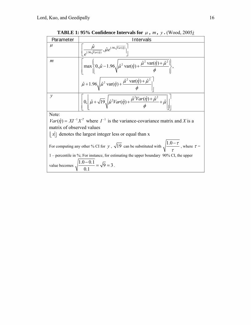
COMPUTATION OF CONFIDENCE INTERVALS Confidence intervals are important to assess the uncertainty associated point estimates of predictive models. Wood (17) proposed a method for estimating the confidence intervals for the mean response ( ), for the gamma mean ( m ), and the predicted response ( y ) at a new site having similar characteristics as the sites used in the original dataset from which the model was developed. For Poisson-gamma models, the 95% confidence intervals for , m and y are described in Table 1. In this table, η is the logarithm of the

estimated mean response µ, while ( 1 ) is the inverse dispersion parameter of the Poisson-gamma model, as described above. In this paper, the confidence intervals were only estimated for the predicted value (y), since the technique proposed in the HSM applies only to predicted values. Furthermore, the confidence intervals were estimated

using the varying dispersion parameter, 0

1

e L , for the full models (18). It should be

pointed out that NB models estimated using a varying dispersion parameter predicts narrower confidence intervals than one estimated using a fixed dispersion parameter (19). COMPUTING THE PRODUCT OF RANDOM VARIABLES Using the theory related to the multiplication of independent random variables (20, 21), Lord (6) proposed a method to estimate the variance and associated confidence intervals for the product of baseline models and AMFs. This theory on which this method is based states that the equations presented below will be exact independent of the type of distribution to which each random variable belongs. For the purpose of this description, z will be defined as the product of independent random variables:

321 xxxz (5)

where,


z = the product of independent random variables; and, sx' = random variable taken from any kind of distribution. It should be pointed out that the mean and variance estimates are defined as E x

and 2E x (second central moment), respectively.

Mean of a Product The mean of the product is the direct application of Equation (5):

321 xxxz

321 xExExEzE (6)

1 2 3z x x x

The mean or average of the product is simply the product of the mean value of the random variables. Variance of a Product The variance of a product is obtained by taking the expectation square of z :

23

22

21

2 xxxz

23

22

21

2 xExExEzE (7)

2 2 2 21 1 2 2 3 3z z x x x x x x

Note: nnE x E x ;

for 2n , 22E x E x 2 2 22E x E x E .

The variance z is computed by first calculating the product on the right hand side and

then subtracting the square of the mean 2z computed in Equation (7):

2 2 2 21 1 2 2 3 3z x x x x x x z (8)

Note that if all 'x s equal zero, the variance z will also equal zero:

2 2 2 21 2 3

2 2 0

z x x x z

z z z


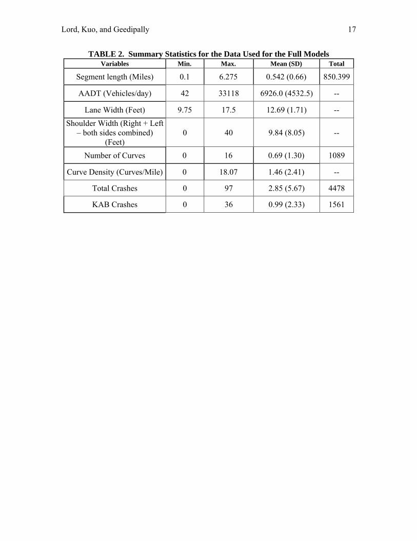
The reader is referred to Lord (6) for additional information about how apply Equations (5 – 8) in the product of a baseline model and AMFs. The paper also describes an example about how to apply the theory. DATA CHARACTERISTICS This section describes the characteristics of the data used for estimating the full and baseline models. The data were collected in Texas (1997-2001) and in Washington State (1999-2002). The data were obtained from the Department of Public Safety (DPS) and the Texas Department of Transportation (TxDOT) for Texas and from the Highway Safety Information System (HSIS) (www.hsis.org) managed by the University of North Carolina on behalf of the Federal Highway Administration for the State of Washington. 1,570 undivided segments were used for developing the full models and the summary statistics are shown in Table 2. Additional information about the characteristics of the data can be found in the final NCHRP 17-29 report (7).

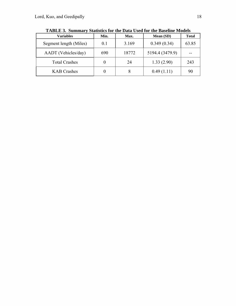
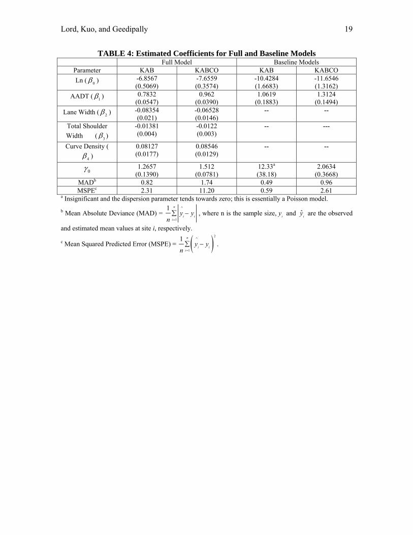
Baseline models are developed using a given set of baseline conditions. The baseline conditions usually reflect the nominal conditions agencies most often used for designing segments and intersections. In this study, nominal baseline conditions used for segments were paved 11-12 ft lanes, 7-8 ft shoulder widths and no horizontal curves (i.e., only tangents). To increase the sample size (at the request of the NCHRP advisory panel), lane widths of 11ft and 12ft and shoulder widths of 7ft and 8ft were combined together. A total of 183 segments were used for developing baseline models and the summary statistics are shown in Table 3. It should be pointed out that baseline models can also be estimated by inputting the nominal value for each element other than flow in the full model. This method is more useful when the sample size of the data is limited, but has not been found to be better than estimating baseline models from data meeting nominal conditions (22). MODELING RESULTS AND AMFS This section describes the modeling results. The coefficients of the models were estimated using the PROC NLMIXED function in SAS (23). The functional forms used for the models were as follows:

Full Model: 2 2 3 3 4 410

x x xLF e

Baseline Model: 10LF

Dispersion parameter: 0

1

e L


Table 4 summarizes the modeling results for KABCO and KAB models. The model results show that increasing lane and shoulder widths decreases the number of crashes, while adding horizontal curves on segments increases the number of crashes.

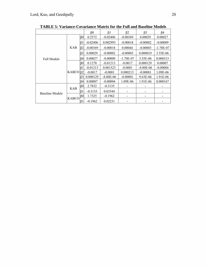
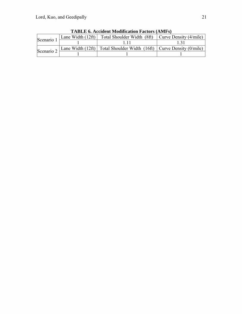
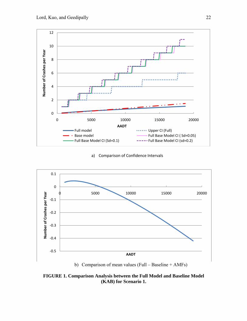
Table 5 shows the characteristics of the variance-covariance matrix. The inverse of that matrix is needed for computing the predicted confidence intervals. Table 6 summarizes the three AMFs used for the two scenarios. The AMFs were taken from the original NCHRP 17-29 report. Since the AMFs do not have standard errors, three hypothetical standard deviation values were used for each AMF: 0.05 (small variance), 0.10 (medium variance), 0.20 (large variance). The objective was to investigate how sensitive were the AMF values for computing the variance of the predicted number of crashes. It should be pointed out that for all three standard deviation values, the AMF could actually lead to an increase in the number of crashes, since the upper bound of the 95% confidence interval crosses the value 1. The next section presents the analysis results. COMPARISON ANALYSIS This section describes the results of the comparison analysis. The results are summarized for each scenario. SCENARIO 1 − 12-ft lanes, 8-ft shoulders, 4 curves/mile Figure 1 shows the comparison analysis for the KAB models. Figure 1a shows the 95% CI for the predicted value, while Figure 1b illustrates the absolute difference between the mean of the full model and the product between the baseline model and AMFs as a function of AADT. The figure shows that the product of the baseline model and AMFs predicts more crashes than that the full model for traffic volumes above 5,500 vehicles per day. Even though the difference appears to be large in Figure 1b), the true picture of the difference is seen in Figure 1a). This figure also illustrates that the 95% CI for the predicted values is much smaller for the full model, especially for vehicular traffic above 2,500 vehicles per day.

Figure 2 shows the comparison analysis for the KABCO models for the first scenario. Figure 2a shows the 95% CI for the predicted value, while Figure 2b illustrates the absolute difference between the mean of the full model and the product between the baseline model and AMFs as a function of AADT. Similar to KAB modeling output, Figure 2 shows that the product of the baseline model and AMFs predicts more crashes than that the full model for traffic volumes above 7,000 vehicles per day. Interestingly,


the 95% CI for the KABCO baseline model combined with AMFs is actually much smaller for traffic flow below 5,000 vehicles per day.

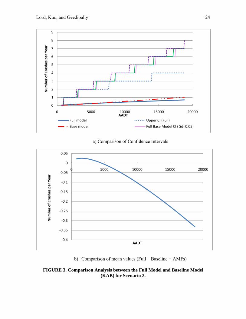
SCENARIO 2 − 12-ft lanes, 12-ft shoulder width, and 1 curve/mile Figure 3 shows the comparison analysis for the KAB models for the second scenario. Figure 3a shows the 95% CI for the predicted value; Figure 3b illustrates the absolute difference between the mean of the full model and the product between the baseline model and AMFs as a function of AADT. Again, the figure shows that the product of the baseline model and AMFs predicts more crashes than that the full model for traffic volumes above 5,000 vehicles per day. This figure also illustrates that the 95% CI for the predicted values is much smaller for the full the model for the entire range of vehicular traffic.

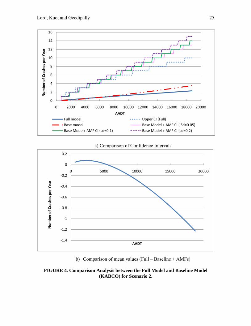
Figure 4 shows the comparison analysis for the KABCO models for the second scenario. This figure shows that the product of the baseline model and AMFs predicts much more crashes than that the full model for traffic volumes above 5,000 vehicles per day. This figure also illustrates that the 95% CI for the predicted values is much smaller for the full the model, especially for vehicular traffic above 3,000 vehicles per day.

DISCUSSION The comparison analysis detailed above provided very interesting results. First, the results show that the 95% CIs for the predicted values have, in general, much wider boundaries for the product of the baseline models and AMFs than those produced by the full models. This difference gets larger as the traffic flow increases. The difference in the width of the boundaries could be as high as 122%. However, it should be noted that for low traffic volumes (less than 5,000 vehicle per day), the boundaries for the full models were larger than those produced by the baseline combined with AMFs. This is explained by the low predicted values of the baseline models used in Equation 8.

To follow on the first point, the results indicate that the variance produced by the uncertainty associated with the AMFs significantly increases the variance produced from the product of these factors with the baseline models. This was noted for all three standard deviation values used in the two scenarios: 0.05, 0.10 and 0.20. To illustrate this characteristic, an example is shown below. The example used the KABCO models applied in the first scenario for 15,000 vehicles per day and the standard error equal to 0.10 for each AMF. Using the equations described above, the variance for the two types of models can be computed as follows: Full Model: 4.71Full (from Table 1)

Baseline Model: 3.67baseline (from Table 1)


Baseline Model+ AMFs:

2 2 2 2 2

2 2 2

2.62 3.67 1 0.1 1.11 0.1

1.31 0.1 3.82 8.30

baseline AMFs

(from Equation 8)

This example shows that the variance associated with the full model is slightly higher than the one estimated from the baseline model, as expected. By including the AMFs, the final variance is increased by about 76% (note: the full model also includes the same variables as the AMFs; yet, the final variance is much smaller). Thus, every new AMF added to the baseline model has an important influence on the final variance of the product, confirming the results provided by Lord (6).

Third, when the 95% CI is included in the analysis, the prediction produced by the product of the baseline model and AMFs is not statistically different form the one produced by the full model. This means that in terms of prediction, both approaches could be used, if the study objective only consists of estimating the mean value of the prediction. However, if one is interested using the model having the smallest variance for decision-making process, hence smaller 95% CIs, the full model should be used over the baseline model combined with AMFs. The lead author recently participated in a seminar for training practitioners about the applications of AMFs in safety analyses. Interestingly, the participants indicated that providing the best and worst case scenarios (i.e., 95% CI) was the most important criterion when AMFs are used as part of these analyses.

In summary, the study outcome shows that models with covariates are preferable over the application of baseline models and AMFs when uncertainty is part of the decision-making process. However, as discussed by Persaud et al. (3) and Lord and Bonneson (4), full models can be very difficult to recalibrate when they are estimated in a given jurisdiction are applied to another jurisdiction. SUMMARY AND CONCLUSIONS

The objective of this research consisted in evaluating the application of full models and baseline models combined with AMFs for predicting motor vehicle crashes. The analysis focused on the predicted values and associated inferences for both types of model. The prediction of crashes will be one of the methodologies proposed in the forthcoming HSM. At this point in time, the recommended predictive methodology is to use baseline models combined with AMFs. In order to compare the models, full and baseline models were estimated using data collected on rural four-lane highways in Texas; these data were originally assembled for the NCHRP 17-29 research project. AMFs describing the safety effects of lane and shoulder widths as well as the number of horizontal curves per mile were also extracted from that work. Regression models were estimated for all and serious injuries crashes. Then, the two types of model were compared as a function of the predicted values, the 95% predicted CIs and different standard deviations to characterize the uncertainty associated with each AMF. Two scenarios with different values of AMFs were evaluated.

The results of this study show that the product of baseline models and AMFs produce much wider 95% predicted CIs than the ones calculated using the full models, except at low traffic flow volumes. This was consistent for the two scenarios evaluated


and for all levels of uncertainty associated with the AMFs. The width of the lower and upper boundaries becomes increasingly larger as traffic flow increases. Considering the uncertainty associated predicted values, both types of model can be used to predict motor vehicle crashes. However, if the study objective includes minimizing the variance associated with the prediction, then the full model should be used over the product of the baseline model and AMFs, since the former produces much smaller variance. Further work includes looking at the effects of adding several AMFs to baseline models; in this work, only three were applied. A new method to re-calibrate full models should also be investigated, if full models become the proposed predictive methodology in a future edition of the HSM. ACKNOWLEDGEMENTS This paper benefited from the input of three anonymous reviewers. Their comments and suggestions are greatly acknowledged. References 1 Hughes, W., K. Eccles, D. Harwood, I. Potts, and E. Hauer (2005) Development of a

Highway Safety Manual. Appendix C: Highway Safety Manual Prototype Chapter: Two- Lane Highways. NCHRP Web Document 62 (Project 17-18(4)). Washington, D.C. (http://onlinepubs.trb.org/onlinepubs/nchrp/nchrp_w62.pdf, accessed October 2007)

2 Transportation Research Board (TRB). (2000). Highway capacity manual, National

Research Concil, TRB, Washington, D.C. 3 Persaud, B.N., D. Lord, and J. Palminaso (2002) Issues of calibration and

transferability in developing accident prediction models for urban intersections. Transportation Research Record 1784, 57-64.

4 Lord, D., and J.A. Bonneson (2005) Calibration of Predictive Models for Estimating

the Safety of Ramp Design Configurations. Transportation Research Record 1908, pp. 88-95.

5 Barreto, H., and F.M. Howland (2005) Introductory Econometrics: Using Monte

Carlo Simulation with Microsoft Excel. Cambridge University Press, New York, N.Y.

6 Lord, D. (2008) Methodology for Estimating the Variance and Confidence Intervals

of the Estimate of the Product of Baseline Models and AMFs. Accident Analysis & Prevention, Vol. 40, No. 3, pp. 1013-1017.

7 Lord, D., Geedipally, S.R., Persaud, B.N., Washington, S.P., van Schalkwyk, I., Ivan,

J.N., Lyon, C., Jonsson, T. ( 2008) Methodology for estimating the safety


performance of multilane rural highways. NCHRP Web-Only Document 126, National Cooperation Highway Research Program, Washington, D.C.

8 Lord, D. (2006) Modeling motor vehicle crashes using Poisson-gamma models:

Examining the effects of low sample mean values and small sample size on the estimation of the fixed dispersion parameter. Accident Analysis & Prevention, Vol. 38, No. 4, pp. 751-766.

9 Lord, D., and F. Mannering (2010) The Statistical Analysis of Crash-Frequency Data: A Review and Assessment of Methodological Alternatives. Transportation Research, Part A, in press. (DOI: 10.1016/j.tra.2010.02.001)

10 Lord, D., S.D. Guikema, and S. Geedipally (2008) Application of the Conway-

Maxwell- Poisson Generalized Linear Model for Analyzing Motor Vehicle Crashes. Accident Analysis & Prevention, Vol. 40, No. 3, pp. 1123-1134.

11 Xie, Y., D. Lord, and Y. Zhang (2007) Predicting Motor Vehicle Collisions using

Bayesian Neural Networks: An Empirical Analysis. Accident Analysis & Prevention, Vol. 39, No. 5, pp. 922-933.

12 Cameron, A.C., and P.K. Trivedi (1998) Regression analysis of count data,

Econometric Society Monograph No.30, Cambridge University Press, New York, N.Y.

13 Maher M.J., and I. Summersgill (1996) A Comprehensive Methodology for the

Fitting Predictive Accident Models. Accident Analysis & Prevention, Vol. 28, No. 3, pp. 281-296.

14 Smyth, G. K. (1989) Generalized linear models with varying dispersion. J.R. Statist.

Soc.B, 51, pp. 47-60. 15 Heydecker, B.G., J. Wu (2001) Identification of Sites for Road Accident Remedial

Work by Bayesien Statistical Methods: An Example of Uncertain Inference. Advances in Engineering Software, Vol. 32, pp. 859-869.

16 Hilbe, J.M. (2007) Negative Binomial Regression. Cambridge University Press, New

York, N.Y. 17 Wood, G.R.( 2005) Confidence and prediction intervals for generalized linear

accident models. Accident Analysis & Prevention 37 (2), 267-273. 18 Miaou, S.-P., and D. Lord (2003) Modeling Traffic-Flow Relationships at Signalized

Intersections: Dispersion Parameter, Functional Form and Bayes vs Empirical Bayes. Transportation Research Record 1840, pp. 31-40.


19 Geedipally, S.R., Lord, D. (2008) Effects of the varying dispersion parameter of Poisson gamma models on the estimation of confidence intervals of crash prediction models. Transportation Research Record 2061, 46-54.

20 Ang, A. H.-S., and W.H. Tang (1975) Probability Concepts in Engineering Planning

and Design: Basic Principles (Vol. 1), John Wiley & Sons, New York, N.Y. 21 Browne, J.M. (2000) Probabilistic Design. Class Notes, School of Engineering and

Science Swinburne University of Technology, Hawthorn, Australia. http://www.ses.swin.edu.au/homes/browne/probabilisticdesign/coursenotes/notespdf/4ProbabilisticDesign.pdf.

22 Persaud, B., C. Lyon, and J. Zegeer (2007) Draft executive summary report on research to address Independent Review Group (IRG) issues for the proposed Chapter 8, Highway Safety Manual. Unpublished document submitted for the HSM Task Force, Toronto, Ont.

23 SAS Institute Inc. (2002) Version 9 of the SAS System for Windows, SAS Institute, Cary, NC.


TABLE 1: 95% Confidence Intervals for , m , y . (Wood, 2005) TABLE 2. Summary Statistics for the Data Used for the Full Models TABLE 3. Summary Statistics for the Data Used for the Baseline Models TABLE 4: Estimated Coefficients for Full and Baseline Models TABLE 5: Variance-Covariance Matrix for the Full and Baseline Models FIGURE 1. Comparison Analysis between the Full Model and Baseline Model (KAB) for Scenario 1. FIGURE 2. Comparison Analysis between the Full Model and Baseline Model (KABCO) for Scenario 1. FIGURE 3. Comparison Analysis between the Full Model and Baseline Model (KAB) for Scenario 2. FIGURE 4. Comparison Analysis between the Full Model and Baseline Model (KABCO) for Scenario 2.


TABLE 1: 95% Confidence Intervals for , m , y . (Wood, 2005)

Parameter Intervals

ˆ1.96 ( )

ˆ1.96 ( )

ˆˆ, Var

Vare

e

m 2 22

2 22

ˆˆ ˆvar( )ˆˆ ˆmax 0, 1.96 var( ) ,

ˆˆ ˆvar( )ˆˆ ˆ1.96 var( )

y 2 22 ˆˆ ˆ( )

ˆˆ ˆ ˆ0, 19 ( )Var

Var

Note: TXXIVar 1)ˆ( where 1I is the variance-covariance matrix and X is a

matrix of observed values x denotes the largest integer less or equal than x

For computing any other % CI for y , 19 can be substituted with 1.0

, where =

1 – percentile in %; For instance, for estimating the upper boundary 90% CI, the upper

value becomes 1.0 0.1

9 30.1

.


TABLE 2. Summary Statistics for the Data Used for the Full Models Variables Min. Max. Mean (SD) Total

Segment length (Miles) 0.1 6.275 0.542 (0.66) 850.399

AADT (Vehicles/day) 42 33118 6926.0 (4532.5) --

Lane Width (Feet) 9.75 17.5 12.69 (1.71) --

Shoulder Width (Right + Left – both sides combined)

(Feet) 0 40 9.84 (8.05) --

Number of Curves 0 16 0.69 (1.30) 1089

Curve Density (Curves/Mile) 0 18.07 1.46 (2.41) --

Total Crashes 0 97 2.85 (5.67) 4478

KAB Crashes 0 36 0.99 (2.33) 1561


TABLE 3. Summary Statistics for the Data Used for the Baseline Models Variables Min. Max. Mean (SD) Total

Segment length (Miles) 0.1 3.169 0.349 (0.34) 63.85

AADT (Vehicles/day) 690 18772 5194.4 (3479.9) --

Total Crashes 0 24 1.33 (2.90) 243

KAB Crashes 0 8 0.49 (1.11) 90


TABLE 4: Estimated Coefficients for Full and Baseline Models Full Model Baseline Models

Parameter KAB KABCO KAB KABCO

Ln ( 0 ) -6.8567 (0.5069)

-7.6559 (0.3574)

-10.4284 (1.6683)

-11.6546 (1.3162)

AADT ( 1 ) 0.7832 (0.0547)

0.962 (0.0390)

1.0619 (0.1883)

1.3124 (0.1494)

Lane Width ( 2 ) -0.08354 (0.021)

-0.06528 (0.0146)

-- --

Total Shoulder

Width�� ( 3 )

-0.01381 (0.004)

-0.0122 (0.003)

-- ---

Curve Density (

4 )

0.08127 (0.0177)

0.08546 (0.0129)

-- --

0 1.2657 (0.1390)

1.512 (0.0781)

12.33a (38.18)

2.0634 (0.3668)

MADb 0.82 1.74 0.49 0.96 MSPEc 2.31 11.20 0.59 2.61

a Insignificant and the dispersion parameter tends towards zero; this is essentially a Poisson model.

b Mean Absolute Deviance (MAD) = 1

1 n

i ii

y yn

, where n is the sample size,i

y and ˆi

y are the observed

and estimated mean values at site i, respectively.

c Mean Squared Predicted Error (MSPE) = 2

1

1 n

i ii

y yn

.


TABLE 5: Variance-Covariance Matrix for the Full and Baseline Models

β0 β1 β2 β3 β4

Full Models

KAB

β0 0.2572 -0.02406 -0.00369 0.00029 0.00027

β1 -0.02406 0.002993 -0.00018 -0.00002 -0.00009

β2 -0.00369 -0.00018 0.00044 -0.00003 -1.70E-07

β3 0.00029 -0.00002 -0.00003 0.000019 3.55E-06

β4 0.00027 -0.00009 -1.70E-07 3.55E-06 0.000313

KABCO

β0 0.1278 -0.01213 -0.0017 0.000129 0.00007 β1 -0.01213 0.001523 -0.0001 -8.80E-06 -0.00004 β2 -0.0017 -0.0001 0.000213 -0.00001 1.09E-06 β3 0.000129 -8.80E-06 -0.00001 9.63E-06 1.91E-06 β4 0.00007 -0.00004 1.09E-06 1.91E-06 0.000167

Baseline Models

KAB β0 2.7832 -0.3135 - - -

β1 -0.3135 0.03544 - - -

KABCO β0 1.7325 -0.1962 - - -

β1 -0.1962 0.02231 - - -


TABLE 6. Accident Modification Factors (AMFs)

Scenario 1 Lane Width (12ft) Total Shoulder Width (8ft) Curve Density (4/mile)

1 1.11 1.31

Scenario 2 Lane Width (12ft) Total Shoulder Width (16ft) Curve Density (0/mile)

1 1 1


a) Comparison of Confidence Intervals

b) Comparison of mean values (Full – Baseline + AMFs)

FIGURE 1. Comparison Analysis between the Full Model and Baseline Model

(KAB) for Scenario 1.

0

2

4

6

8

10

12

0 5000 10000 15000 20000

Number of Crashes per Year

AADTFull model Upper CI (Full)

Base model Full Base Model CI ( Sd=0.05)Full Base Model CI (Sd=0.1) Full Base Model CI (sd=0.2)

‐0.5

‐0.4

‐0.3

‐0.2

‐0.1

0

0.1

0 5000 10000 15000 20000


AADT




FIGURE 2. Comparison Analysis between the Full Model and Baseline Model (KABCO) for Scenario 1.

0

2

4

6

8

10

12

14

16

18

20

22

0 5000 10000 15000 20000


AADT

Full model Upper CI (Full)Base model Base Model CI ( Sd=0.05)Base Model CI (Sd=0.1) Base Model CI (sd=0.2)

‐1.8

‐1.6

‐1.4

‐1.2

‐1

‐0.8

‐0.6

‐0.4

‐0.2

0

0.2

0.4

0 5000 10000 15000 20000


AADT




FIGURE 3. Comparison Analysis between the Full Model and Baseline Model (KAB) for Scenario 2.

0

1

2

3

4

5

6

7

8

9

0 5000 10000 15000 20000


AADTFull model Upper CI (Full)

Base model Full Base Model CI ( Sd=0.05)

‐0.4

‐0.35

‐0.3

‐0.25

‐0.2

‐0.15

‐0.1

‐0.05

0

0.05

0 5000 10000 15000 20000


AADT




FIGURE 4. Comparison Analysis between the Full Model and Baseline Model (KABCO) for Scenario 2.

0

2

4

6

8

10

12

14

16

0 2000 4000 6000 8000 10000 12000 14000 16000 18000 20000


AADT

Full model Upper CI (Full)

Base model Base Model + AMF CI ( Sd=0.05)

Base Model+ AMF CI (sd=0.1) Base Model + AMF CI (sd=0.2)

‐1.4

‐1.2

‐1

‐0.8

‐0.6

‐0.4

‐0.2

0

0.2

0 5000 10000 15000 20000


AADT

Documents

Comparing the Application of the Product of Baseline Models and Accident Modification ... · 2010-03-22 · Comparing the Application of the Product of Baseline Models and Accident