Comparative Protein Structure Analysis with Bio3DXin-Qiu Yao, Lars Skjaerven & Barry J. Grant

October 30, 2014 (last updated: Febuary 20, 2015)

Contents

Background 2

Requirements . . . . . . . . . . . . . . . . . . . . . . . . . . . . . . . . . . . . . . . . . . . . . . . . 2

1 Getting Started 2

1.1 Working with single PDB structures . . . . . . . . . . . . . . . . . . . . . . . . . . . . . . . . 2

1.2 Working with multiple PDB structures . . . . . . . . . . . . . . . . . . . . . . . . . . . . . . . 5

1.3 Exploring example data for the transducin heterotrimeric G Protein . . . . . . . . . . . . . . 6

2 Constructing Experimental Structure Ensembles for a Protein Family 7

2.1 Finding Available Sets of Similar Structures . . . . . . . . . . . . . . . . . . . . . . . . . . . . 7

2.2 Multiple Sequence Alignment . . . . . . . . . . . . . . . . . . . . . . . . . . . . . . . . . . . . 9

3 Comparative Structure Analysis 9

3.1 Structure Superposition . . . . . . . . . . . . . . . . . . . . . . . . . . . . . . . . . . . . . . . 10

3.2 Standard Structural Analysis . . . . . . . . . . . . . . . . . . . . . . . . . . . . . . . . . . . . 12

4 Principal Component Analysis (PCA) 17

4.1 Conformer Clustering in PC Space . . . . . . . . . . . . . . . . . . . . . . . . . . . . . . . . . 22

5 Where to Next 24

Document Details 25

Information About the Current Bio3D Session 25

References 25

1

Background

Bio3D1 is an R package that provides interactive tools for the analysis of bimolecular structure, sequenceand simulation data. The aim of this document, termed a vignette2 in R parlance, is to provide a brieftask-oriented introduction to facilities for analyzing protein structure data with Bio3D (Grant et al. 2006).

Requirements

Detailed instructions for obtaining and installing the Bio3D package on various platforms can be found in theInstalling Bio3D vignette available online. Note that to follow along with this vignette the MUSCLE multiplesequence alignment program must be installed on your system and in the search path for executables. Pleasesee the installation vignette for full details. This particular vignette was generated using Bio3D version2.2.0.

1 Getting Started

Start R, load the Bio3D package and use the command demo("pdb") and then demo("pca") to get a quickfeel for some of the tasks that we will be introducing in the following sections.

library(bio3d)demo("pdb")demo("pca")

Side-note: You will be prompted to hit the RETURN key at each step of the demos as this will allow youto see the particular functions being called. Also note that detailed documentation and example code foreach function can be accessed via the help() and example() commands (e.g. help(read.pdb)). You canalso copy and paste any of the example code from the documentation of a particular function, or indeed thisvignette, directly into your R session to see how things work. You can also find this documentation online.

1.1 Working with single PDB structures

A comprehensive introduction to working with PDB format structures with Bio3D can be found in PDBstructure manipulation and analysis vignette. Here we confine ourselves to a very brief overview. Thecode snippet below calls the read.pdb() function with a single input argument, the four letter Protein DataBank (PDB) identifier code "1tag". This will cause the read.pdb() function to read directly from the onlineRCSB PDB database and return a new object pdb for further manipulation.

pdb <- read.pdb("1tag")

## Note: Accessing on-line PDB file## HEADER GTP-BINDING PROTEIN 23-NOV-94 1TAG

Alternatively, you can read a PDB file directly from your local file system using the file name (or the fullpath to the file) as an argument to read.pdb():

1The latest version of the package, full documentation and further vignettes (including detailed installation instructions) canbe obtained from the main Bio3D website: http://thegrantlab.org/bio3d/

2This vignette contains executable examples, see help(vignette) for further details.

2

pdb <- read.pdb("myfile.pdb")pdb <- read.pdb("/path/to/my/data/myfile.pdb")

A short summary of the pdb object can be obtained by calling the function print.pdb() (or simply typingpdb, which is equivalent in this case):

pdb

#### Call: read.pdb(file = "1tag")#### Total Models#: 1## Total Atoms#: 2890, XYZs#: 8670 Chains#: 1 (values: A)#### Protein Atoms#: 2521 (residues/Calpha atoms#: 314)## Nucleic acid Atoms#: 0 (residues/phosphate atoms#: 0)#### Non-protein/nucleic Atoms#: 369 (residues: 342)## Non-protein/nucleic resid values: [ GDP (1), HOH (340), MG (1) ]#### Protein sequence:## ARTVKLLLLGAGESGKSTIVKQMKIIHQDGYSLEECLEFIAIIYGNTLQSILAIVRAMTT## LNIQYGDSARQDDARKLMHMADTIEEGTMPKEMSDIIQRLWKDSGIQACFDRASEYQLND## SAGYYLSDLERLVTPGYVPTEQDVLRSRVKTTGIIETQFSFKDLNFRMFDVGGQRSERKK## WIHCFEGVTCIIFIAALSAYDMVLVEDDEVNRMHESLHLFNSICN...<cut>...DIII#### + attr: atom, helix, sheet, seqres, xyz,## calpha, remark, call

To examine the contents of the pdb object in more detail we can use the attributes function:

attributes(pdb)

## $names## [1] "atom" "helix" "sheet" "seqres" "xyz" "calpha" "remark" "call"#### $class## [1] "pdb" "sse"

These attributes describe the list components that comprise the pdb object, and each individual component canbe accessed using the $ symbol (e.g. pdb$atom). Their complete description can be found on the read.pdb()functions help page accessible with the command: help(read.pdb). Note that the atom component is a dataframe (matrix like object) consisting of all atomic coordinate ATOM/HETATM data, with a row per ATOMand a column per record type. The column names can be used as a convenient means of data access, forexample to access coordinate data for the first three atoms in our newly created pdb object:

pdb$atom[1:3, c("resno","resid","elety","x","y","z")]

## resno resid elety x y z## 1 27 ALA N 38.238 18.018 61.225## 2 27 ALA CA 38.552 16.715 60.576## 3 27 ALA C 40.042 16.687 60.253

3

In the example above we used numeric indices to access atoms 1 to 3, and a character vector of column namesto access the specific record types. In a similar fashion the atom.select() function returns numeric indicesthat can be used for accessing desired subsets of the pdb data. For example:

ca.inds <- atom.select(pdb, "calpha")

The returned ca.inds object is a list containing atom and xyz numeric indices corresponding to the selection(all C-alpha atoms in this particular case). The indices can be used to access e.g. the Cartesian coordinates ofthe selected atoms (pdb$xyz[, ca.inds$xyz]), or residue numbers and B-factor data for the selected atoms.For example:

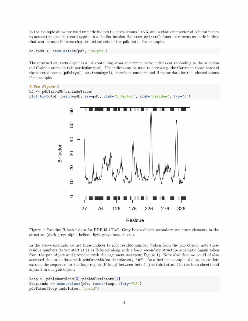
# See Figure 1bf <- pdb$atom$b[ca.inds$atom]plot.bio3d(bf, resno=pdb, sse=pdb, ylab="B-factor", xlab="Residue", typ="l")

010

2030

4050

60

27 76 126 176 226 276 326

Residue

B−

fact

or

Figure 1: Residue B-factor data for PDB id 1TAG. Grey boxes depict secondary structure elements in thestructure (dark grey: alpha helices; light grey: beta sheets).

In the above example we use these indices to plot residue number (taken from the pdb object, note theseresidue numbers do not start at 1) vs B-factor along with a basic secondary structure schematic (again takenfrom the pdb object and provided with the argument sse=pdb; Figure 1). Note also that we could of alsoaccessed this same data with pdb$atom$b[ca.inds$atom, "b"]. As a further example of data access letsextract the sequence for the loop region (P-loop) between beta 1 (the third strand in the beta sheet) andalpha 1 in our pdb object.

loop <- pdb$sheet$end[3]:pdb$helix$start[1]loop.inds <- atom.select(pdb, resno=loop, elety="CA")pdb$atom[loop.inds$atom, "resid"]

4

## [1] "LEU" "GLY" "ALA" "GLY" "GLU" "SER" "GLY" "LYS"

In the above example the residue numbers in the sheet and helix components of pdb are accessed and usedin a subsequent atom selection, the output of which is used as indices to extract residue names.

Since Bio3D version 2.1 the xyz component in the PDB object is in a matrix format (as compared to a vectorformat in previous versions). Thus, notice the extra comma in the square bracket operator when accessingCartesian coordinates from the xyz object (pdb$xyz[, ca.inds$xyz]).

Question: How would you extract the one-letter amino acid sequence for the loop region mentioned above?HINT: The aa321() function converts between three-letter and one-letter IUPAC amino acid codes.

Question: How would you select all backbone or sidechain atoms? HINT: see the example section ofhelp(atom.select) and the string option.

Side-note: Consider the combine.select function for combining multiple atom selections. Seehelp(combine.select) and additional vignettes for more details.

Note that if you know a particular sequence pattern or motif characteristic of a region of interest you couldaccess it via a sequence search as follows:

aa <- pdbseq(pdb)aa[ motif.find(".G....GK[ST]", aa )]

## 35 36 37 38 39 40 41 42 43## "L" "G" "A" "G" "E" "S" "G" "K" "S"

1.2 Working with multiple PDB structures

The Bio3D package was designed to specifically facilitate the analysis of multiple structures from bothexperiment and simulation. The challenge of working with these structures is that they are usually different intheir composition (i.e. contain differing number of atoms, sequences, chains, ligands, structures, conformationsetc. even for the same protein as we will see below) and it is these differences that are frequently of mostinterest.

For this reason Bio3D contains extensive utilities to enable the reading and writing of sequence and structuredata, sequence and structure alignment, performing homologous protein searches, structure annotation, atomselection, re-orientation, superposition, rigid core identification, clustering, torsion analysis, distance matrixanalysis, structure and sequence conservation analysis, normal mode analysis across related structures, andprincipal component analysis of structural ensembles. We will demonstrate some of these utilities in thefollowing sections. More comprehensive demonstrations for special tasks, e.g. various operations of PDBstructures, analysis of MD trajectories and normal mode analysis can be found in corresponding vignettes.

Before delving into more advanced analysis lets examine how we can read multiple PDB structures from theRCSB PDB for a particular protein and perform some basic analysis:

# Download some example PDB filesids <- c("1TND_B","1AGR_A","1FQJ_A","1TAG_A","1GG2_A","1KJY_A")raw.files <- get.pdb(ids)

The get.pdb() function will download the requested files, below we extract the particular chains we are mostinterested in with the function pdbsplit() (note these ids could come from the results of a blast.pdb()search as described in subsequent sections). The requested chains are then aligned and their structural datastored in a new object pdbs that can be used for further analysis and manipulation.

5

# Extract and align the chains we are interested infiles <- pdbsplit(raw.files, ids)pdbs <- pdbaln(files)

Below we examine their sequence and structural similarity.

# Calculate sequence identitypdbs$id <- substr(basename(pdbs$id),1,6)seqidentity(pdbs)

## 1TND_B 1AGR_A 1FQJ_A 1TAG_A 1GG2_A 1KJY_A## 1TND_B 1.000 0.693 0.914 1.000 0.690 0.696## 1AGR_A 0.693 1.000 0.779 0.694 0.997 0.994## 1FQJ_A 0.914 0.779 1.000 0.914 0.776 0.782## 1TAG_A 1.000 0.694 0.914 1.000 0.691 0.697## 1GG2_A 0.690 0.997 0.776 0.691 1.000 0.991## 1KJY_A 0.696 0.994 0.782 0.697 0.991 1.000

## Calculate RMSDrmsd(pdbs, fit=TRUE)

## [,1] [,2] [,3] [,4] [,5] [,6]## [1,] 0.000 0.965 0.609 1.283 1.612 2.100## [2,] 0.965 0.000 0.873 1.575 1.777 1.914## [3,] 0.609 0.873 0.000 1.265 1.737 2.042## [4,] 1.283 1.575 1.265 0.000 1.687 1.841## [5,] 1.612 1.777 1.737 1.687 0.000 1.879## [6,] 2.100 1.914 2.042 1.841 1.879 0.000

Question: What effect does setting the fit=TRUE option have in the RMSD calculation? What would theresults indicate if you set fit=FALSE or disparaged this option? HINT: Bio3D functions have various defaultoptions that will be used if the option is not explicitly specified by the user, see help(rmsd) for an exampleand note that the input options with an equals sign (e.g. fit=FALSE) have default values.

1.3 Exploring example data for the transducin heterotrimeric G Protein

A number of example datasets are included with the Bio3D package. The main purpose of including this data(which may be generated by the user by following the extended examples documented within the variousBio3D functions) is to allow users to more quickly appreciate the capabilities of functions that would otherwiserequire extensive data downloads before execution.

For a number of the examples in the current vignette we will utilize the included transducin dataset thatcontains over 50 publicly available structures. This dataset formed the basis of the work described in(Yao and Grant 2013) and we refer the motivated reader to this publication and references therein forextensive background information. Briefly, heterotrimeric G proteins are molecular switches that turn on andoff intracellular signaling cascades in response to the activation of G protein coupled receptors (GPCRs).Receptor activation by extracellular stimuli promotes a cycle of GTP binding and hydrolysis on the G proteinalpha subunit that leads to conformational rearrangements (i.e. internal structural changes) that activatemultiple downstream effectors. The current dataset consists of transducin (including Gt and Gi/o) alphasubunit sequence and structural data and can be accessed with the command attach(transducin):

6

attach(transducin)

Side-note: This dataset can be assembled from scratch with commands similar to those detailed in the nextsection and those listed in section 2.2. Also see help(example.data) for a full description of this datasetscontents.

2 Constructing Experimental Structure Ensembles for a ProteinFamily

Comparing multiple structures of homologous proteins and carefully analyzing large multiple sequencealignments can help identify patterns of sequence and structural conservation and highlight conservedinteractions that are crucial for protein stability and function (Grant et al. 2007). Bio3D provides a usefulframework for such studies and can facilitate the integration of sequence, structure and dynamics data in theanalysis of protein evolution.

2.1 Finding Available Sets of Similar Structures

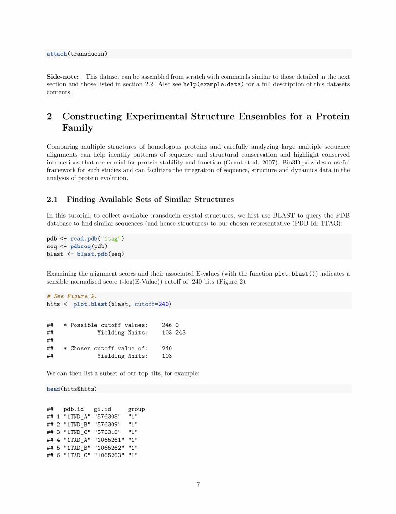
In this tutorial, to collect available transducin crystal structures, we first use BLAST to query the PDBdatabase to find similar sequences (and hence structures) to our chosen representative (PDB Id: 1TAG):

pdb <- read.pdb("1tag")seq <- pdbseq(pdb)blast <- blast.pdb(seq)

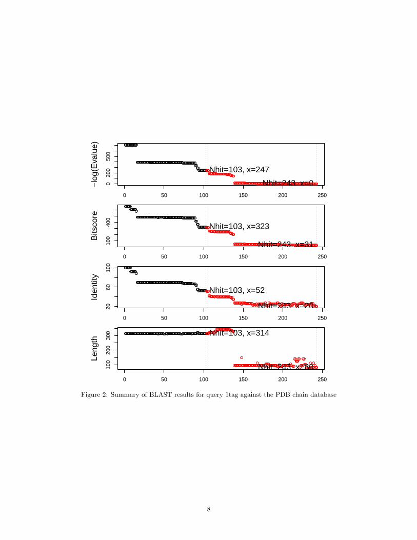
Examining the alignment scores and their associated E-values (with the function plot.blast()) indicates asensible normalized score (-log(E-Value)) cutoff of 240 bits (Figure 2).

# See Figure 2.hits <- plot.blast(blast, cutoff=240)

## * Possible cutoff values: 246 0## Yielding Nhits: 103 243#### * Chosen cutoff value of: 240## Yielding Nhits: 103

We can then list a subset of our top hits, for example:

head(hits$hits)

## pdb.id gi.id group## 1 "1TND_A" "576308" "1"## 2 "1TND_B" "576309" "1"## 3 "1TND_C" "576310" "1"## 4 "1TAD_A" "1065261" "1"## 5 "1TAD_B" "1065262" "1"## 6 "1TAD_C" "1065263" "1"

7

0 50 100 150 200 250

020

050

0

−lo

g(E

valu

e)

Nhit=103, x=247

Nhit=243, x=0

0 50 100 150 200 250

100

400

Bits

core

Nhit=103, x=323

Nhit=243, x=31

0 50 100 150 200 250

2060

100

Iden

tity

Nhit=103, x=52

Nhit=243, x=20

0 50 100 150 200 250

100

200

300

Leng

th

Nhit=103, x=314

Nhit=243, x=80

Figure 2: Summary of BLAST results for query 1tag against the PDB chain database

8

head(hits$pdb.id)

## [1] "1TND_A" "1TND_B" "1TND_C" "1TAD_A" "1TAD_B" "1TAD_C"

Sidenote: The function pdb.annotate() can fetch detailed information about the corresponding structures(e.g. title, experimental method, resolution, ligand name(s), citation, etc.). For example:

anno <- pdb.annotate(hits$pdb.id)head(anno[, c("resolution", "ligandId", "citation")])

## resolution ligandId citation## 1TND_A 2.2 CAC,GSP,MG Noel et al. Nature (1993)## 1TND_B 2.2 CAC,GSP,MG Noel et al. Nature (1993)## 1TND_C 2.2 CAC,GSP,MG Noel et al. Nature (1993)## 1TAD_A 1.7 ALF,CA,CAC,GDP Sondek et al. Nature (1994)## 1TAD_B 1.7 ALF,CA,CAC,GDP Sondek et al. Nature (1994)## 1TAD_C 1.7 ALF,CA,CAC,GDP Sondek et al. Nature (1994)

2.2 Multiple Sequence Alignment

Next we download the complete list of structures from the PDB (with function get.pdb()), and use functionpdbsplit() to split the structures into separate chains and store them for subsequent access. Finally,function pdbaln() will extract the sequence of each structure and perform a multiple sequence alignment todetermine residue-residue correspondences (NOTE: requires external program MUSCLE be in search pathfor executables):

# Download PDBs and split by chain IDfiles <- get.pdb(hits, path="raw_pdbs", split = TRUE)

# Extract and align sequencespdbs <- pdbaln(files)

You can now inspect the alignment (the automatically generated “aln.fa” file) with your favorite alignmentviewer (we recommend SEAVIEW, available from: http://pbil.univ-lyon1.fr/software/seaview.html).

Side-note: You may find a number of structures with missing residues (i.e. gaps in the alignment) at sitesof particular interest to you. If this is the case you may consider removing these structures from your hit listand generating a smaller, but potentially higher quality, dataset for further exploration.

Question: How could you automatically identify gap positions in your alignment? HINT: try the commandhelp.search("gap", package="bio3d").

3 Comparative Structure Analysis

The detailed comparison of homologous protein structures can be used to infer pathways for evolutionaryadaptation and, at closer evolutionary distances, mechanisms for conformational change. The Bio3D packageemploys both conventional methods for structural analysis (alignment, RMSD, difference distance matrixanalysis, etc.) as well as refined structural superposition and principal component analysis (PCA) to facilitatecomparative structure analysis.

9

3.1 Structure Superposition

Conventional structural superposition of proteins minimizes the root mean square difference between theirfull set of equivalent residues. This can be performed with Bio3D functions pdbfit() and fit.xyz() asoutlined previously. However, for certain applications such a superposition procedure can be inappropriate.For example, in the comparison of a multi-domain protein that has undergone a hinge-like rearrangement ofits domains, standard all atom superposition would result in an underestimate of the true atomic displacementby attempting superposition over all domains (whole structure superposition). A more appropriate andinsightful superposition would be anchored at the most invariant region and hence more clearly highlight thedomain rearrangement (sub-structure superposition).

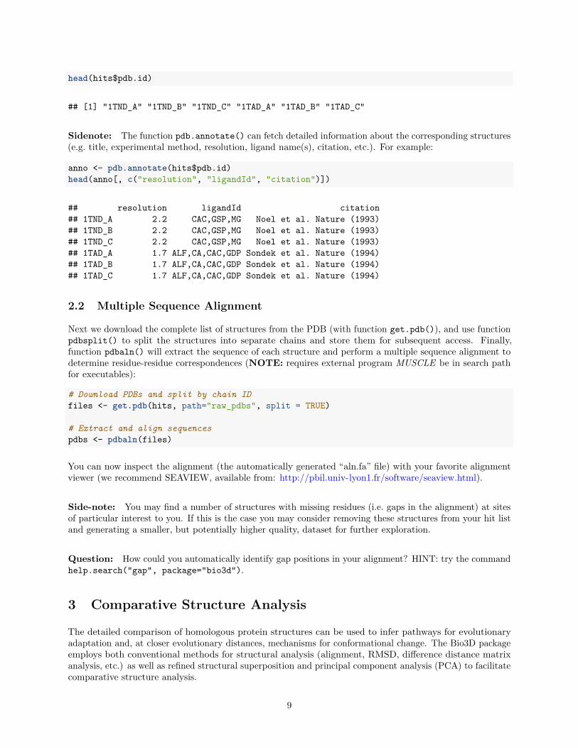
The Bio3D core.find() function implements an iterated superposition procedure, where residues displayingthe largest positional differences are identified and excluded at each round. The function returns an orderedlist of excluded residues, from which the user can select a subset of ’core’ residues upon which superpositioncan be based.

core <- core.find(pdbs)

The plot.core() and print.core() functions allow one to further examine the output of the core.find()procedure (see below and Figure 3).

# See Figure 3.col=rep("black", length(core$volume))col[core$volume<2]="pink"; col[core$volume<1]="red"plot(core, col=col)

304 265 225 185 145 105 65

050

100

150

200

250

Core Size (Number of Residues)

Tota

l Elli

psoi

d V

olum

e (A

ngst

rom

^3)

Figure 3: Identification of core residues

10

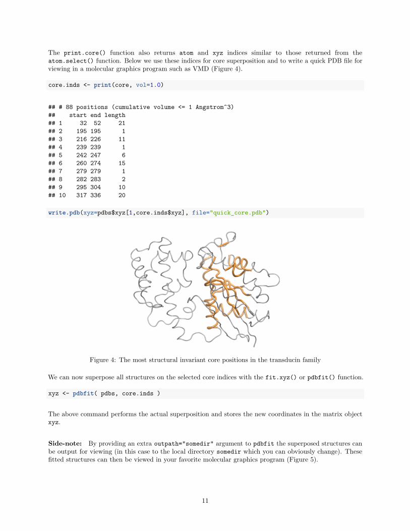
The print.core() function also returns atom and xyz indices similar to those returned from theatom.select() function. Below we use these indices for core superposition and to write a quick PDB file forviewing in a molecular graphics program such as VMD (Figure 4).

core.inds <- print(core, vol=1.0)

## # 88 positions (cumulative volume <= 1 Angstrom^3)## start end length## 1 32 52 21## 2 195 195 1## 3 216 226 11## 4 239 239 1## 5 242 247 6## 6 260 274 15## 7 279 279 1## 8 282 283 2## 9 295 304 10## 10 317 336 20

write.pdb(xyz=pdbs$xyz[1,core.inds$xyz], file="quick_core.pdb")

Figure 4: The most structural invariant core positions in the transducin family

We can now superpose all structures on the selected core indices with the fit.xyz() or pdbfit() function.

xyz <- pdbfit( pdbs, core.inds )

The above command performs the actual superposition and stores the new coordinates in the matrix objectxyz.

Side-note: By providing an extra outpath="somedir" argument to pdbfit the superposed structures canbe output for viewing (in this case to the local directory somedir which you can obviously change). Thesefitted structures can then be viewed in your favorite molecular graphics program (Figure 5).

11

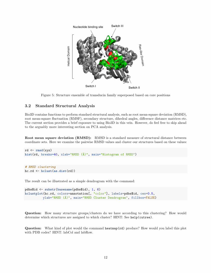
Figure 5: Structure ensemble of transducin family superposed based on core positions

3.2 Standard Structural Analysis

Bio3D contains functions to perform standard structural analysis, such as root mean-square deviation (RMSD),root mean-square fluctuation (RMSF), secondary structure, dihedral angles, difference distance matrices etc.The current section provides a brief exposure to using Bio3D in this vein. However, do feel free to skip aheadto the arguably more interesting section on PCA analysis.

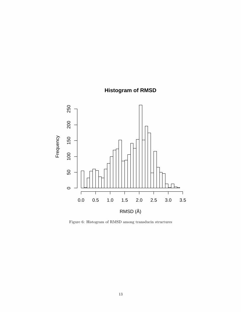
Root mean square deviation (RMSD): RMSD is a standard measure of structural distance betweencoordinate sets. Here we examine the pairwise RMSD values and cluster our structures based on these values:

rd <- rmsd(xyz)hist(rd, breaks=40, xlab="RMSD (Å)", main="Histogram of RMSD")

# RMSD clusteringhc.rd <- hclust(as.dist(rd))

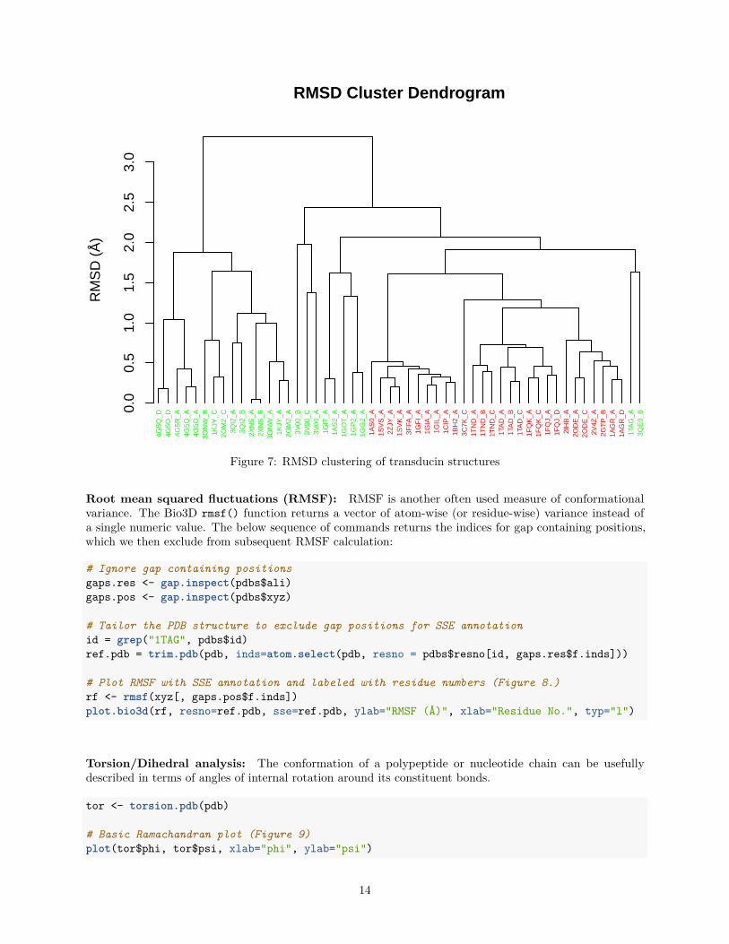
The result can be illustrated as a simple dendrogram with the command:

pdbs$id <- substr(basename(pdbs$id), 1, 6)hclustplot(hc.rd, colors=annotation[, "color"], labels=pdbs$id, cex=0.5,

ylab="RMSD (Å)", main="RMSD Cluster Dendrogram", fillbox=FALSE)

Question: How many structure groups/clusters do we have according to this clustering? How woulddetermine which structures are assigned to which cluster? HINT: See help(cutree).

Question: What kind of plot would the command heatmap(rd) produce? How would you label this plotwith PDB codes? HINT: labCol and labRow.

12

Histogram of RMSD

RMSD (Å)

Fre

quen

cy

0.0 0.5 1.0 1.5 2.0 2.5 3.0 3.5

050

100

150

200

250

Figure 6: Histogram of RMSD among transducin structures

13

RMSD Cluster DendrogramR

MS

D (

Å)

0.0

0.5

1.0

1.5

2.0

2.5

3.0

4G5Q

_D4G

5O_D

4G5R

_A4G

5Q_A

4G5O

_A3O

NW

_B1K

JY_C

2OM

2_C

3QI2

_A3Q

I2_B

2XN

S_A

2XN

S_B

3ON

W_A

1KJY

_A2O

M2_

A3V

00_B

3V00

_C3V

00_A

1GIT

_A1A

S2_

A1G

OT

_A1G

P2_

A1G

G2_

A1A

S0_

A1S

VS

_A2Z

JY_A

1SV

K_A

3FFA

_A1G

FI_

A1G

IA_A

1GIL

_A1C

IP_A

1BH

2_A

3C7K

_C1T

ND

_A1T

ND

_B1T

ND

_C1T

AD

_A1T

AD

_B1T

AD

_C1F

QK

_A1F

QK

_C1F

QJ_

A1F

QJ_

D2I

HB

_A2O

DE

_A2O

DE

_C2V

4Z_A

2GT

P_B

1AG

R_A

1AG

R_D

1TA

G_A

3QE

0_B

Figure 7: RMSD clustering of transducin structures

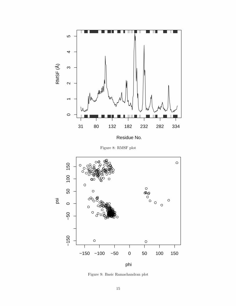
Root mean squared fluctuations (RMSF): RMSF is another often used measure of conformationalvariance. The Bio3D rmsf() function returns a vector of atom-wise (or residue-wise) variance instead ofa single numeric value. The below sequence of commands returns the indices for gap containing positions,which we then exclude from subsequent RMSF calculation:

# Ignore gap containing positionsgaps.res <- gap.inspect(pdbs$ali)gaps.pos <- gap.inspect(pdbs$xyz)

# Tailor the PDB structure to exclude gap positions for SSE annotationid = grep("1TAG", pdbs$id)ref.pdb = trim.pdb(pdb, inds=atom.select(pdb, resno = pdbs$resno[id, gaps.res$f.inds]))

# Plot RMSF with SSE annotation and labeled with residue numbers (Figure 8.)rf <- rmsf(xyz[, gaps.pos$f.inds])plot.bio3d(rf, resno=ref.pdb, sse=ref.pdb, ylab="RMSF (Å)", xlab="Residue No.", typ="l")

Torsion/Dihedral analysis: The conformation of a polypeptide or nucleotide chain can be usefullydescribed in terms of angles of internal rotation around its constituent bonds.

tor <- torsion.pdb(pdb)

# Basic Ramachandran plot (Figure 9)plot(tor$phi, tor$psi, xlab="phi", ylab="psi")

14

01

23

45

31 80 132 182 232 282 334

Residue No.

RM

SF

(Å

)

Figure 8: RMSF plot

−150 −100 −50 0 50 100 150

−15

0−

500

5010

015

0

phi

psi

Figure 9: Basic Ramachandran plot

15

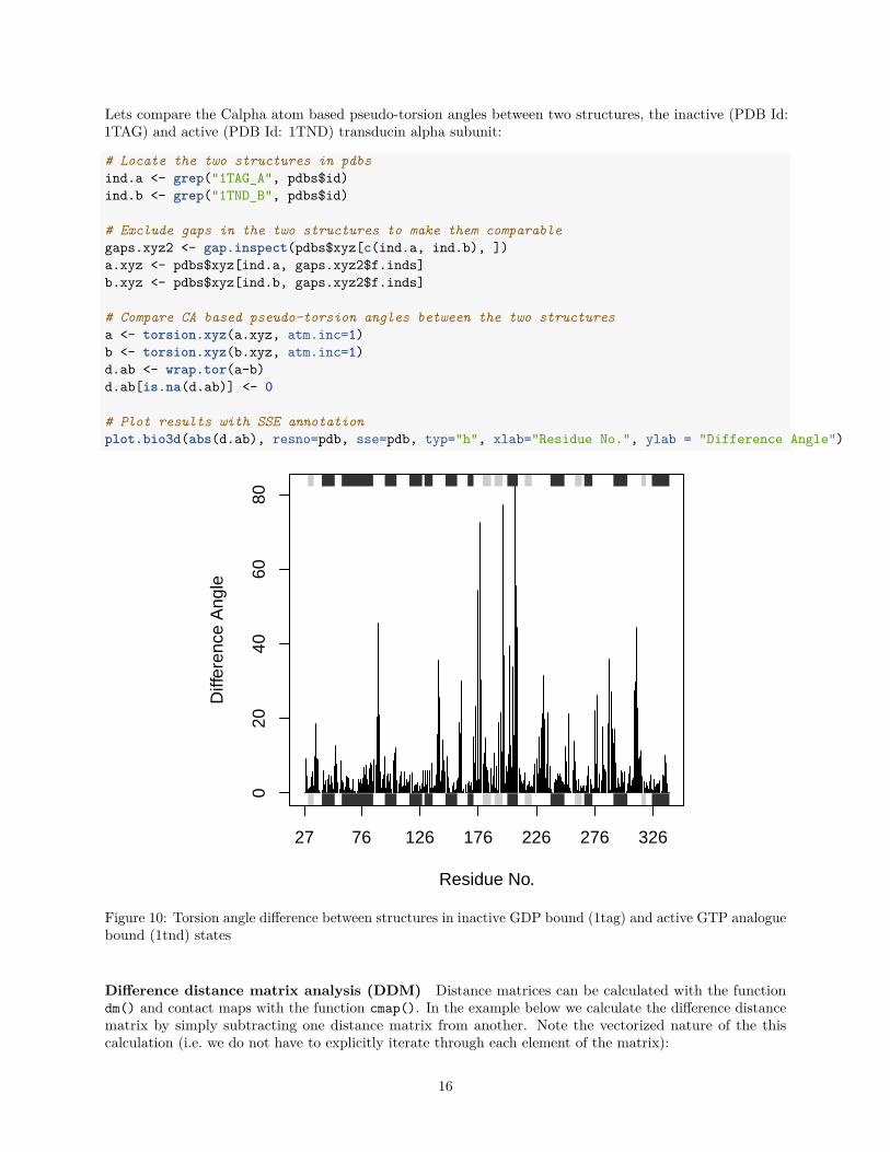
Lets compare the Calpha atom based pseudo-torsion angles between two structures, the inactive (PDB Id:1TAG) and active (PDB Id: 1TND) transducin alpha subunit:

# Locate the two structures in pdbsind.a <- grep("1TAG_A", pdbs$id)ind.b <- grep("1TND_B", pdbs$id)

# Exclude gaps in the two structures to make them comparablegaps.xyz2 <- gap.inspect(pdbs$xyz[c(ind.a, ind.b), ])a.xyz <- pdbs$xyz[ind.a, gaps.xyz2$f.inds]b.xyz <- pdbs$xyz[ind.b, gaps.xyz2$f.inds]

# Compare CA based pseudo-torsion angles between the two structuresa <- torsion.xyz(a.xyz, atm.inc=1)b <- torsion.xyz(b.xyz, atm.inc=1)d.ab <- wrap.tor(a-b)d.ab[is.na(d.ab)] <- 0

# Plot results with SSE annotationplot.bio3d(abs(d.ab), resno=pdb, sse=pdb, typ="h", xlab="Residue No.", ylab = "Difference Angle")

020

4060

80

27 76 126 176 226 276 326

Residue No.

Diff

eren

ce A

ngle

Figure 10: Torsion angle difference between structures in inactive GDP bound (1tag) and active GTP analoguebound (1tnd) states

Difference distance matrix analysis (DDM) Distance matrices can be calculated with the functiondm() and contact maps with the function cmap(). In the example below we calculate the difference distancematrix by simply subtracting one distance matrix from another. Note the vectorized nature of the thiscalculation (i.e. we do not have to explicitly iterate through each element of the matrix):

16

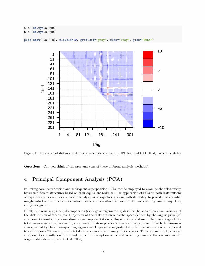
a <- dm.xyz(a.xyz)b <- dm.xyz(b.xyz)

plot.dmat( (a - b), nlevels=10, grid.col="gray", xlab="1tag", ylab="1tnd")

−10

−5

0

5

10

1tag

1tnd

1 41 81 121 181 241 301

301281261241221201181161141121101

81614121

1

Figure 11: Difference of distance matrices between structures in GDP(1tag) and GTP(1tnd) nucleotide states

Question: Can you think of the pros and cons of these different analysis methods?

4 Principal Component Analysis (PCA)

Following core identification and subsequent superposition, PCA can be employed to examine the relationshipbetween different structures based on their equivalent residues. The application of PCA to both distributionsof experimental structures and molecular dynamics trajectories, along with its ability to provide considerableinsight into the nature of conformational differences is also discussed in the molecular dynamics trajectoryanalysis vignette.

Briefly, the resulting principal components (orthogonal eigenvectors) describe the axes of maximal variance ofthe distribution of structures. Projection of the distribution onto the space defined by the largest principalcomponents results in a lower dimensional representation of the structural dataset. The percentage of thetotal mean square displacement (or variance) of atom positional fluctuations captured in each dimension ischaracterized by their corresponding eigenvalue. Experience suggests that 3–5 dimensions are often sufficientto capture over 70 percent of the total variance in a given family of structures. Thus, a handful of principalcomponents are sufficient to provide a useful description while still retaining most of the variance in theoriginal distribution (Grant et al. 2006).

17

The below command excludes the gap positions identified above from the PCA (note you can also simply runpca(xyz, rm.gaps=TRUE)).

# Do PCApc.xray <- pca.xyz(xyz[, gaps.pos$f.inds])pc.xray

#### Call:## pca.xyz(xyz = xyz[, gaps.pos$f.inds])#### Class:## pca#### Number of eigenvalues:## 915#### Eigenvalue Variance Cumulative## PC 1 259.521 49.794 49.794## PC 2 81.302 15.599 65.393## PC 3 40.095 7.693 73.086## PC 4 29.701 5.699 78.785## PC 5 24.048 4.614 83.399## PC 6 19.611 3.763 87.162#### (Obtained from 53 conformers with 915 xyz input values).#### + attr: L, U, z, au, sdev, mean, call

Question: Why is the input to function pca.xyz() given as xyz rather than pdbs$xyz?

Question: Why would you need superposition before using pca.xyz but not need it for pca.tor?

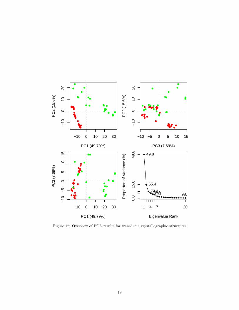
A quick overview of the results of pca.xyz() can be obtained by calling print.pca() and plot.pca()(Figure 12).

plot(pc.xray, col=annotation[, "color"])

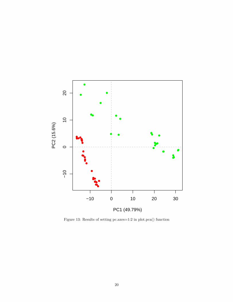
Setting the option pc.axes will allow for single plots to also be produced in this way, e.g.:

plot(pc.xray, pc.axes=1:2, col=annotation[, "color"])

One can then use the identify() function to label and individual points.

# Left-click on a point to label and right-click to endidentify(pc.xray$z[,1:2], labels=basename.pdb(pdbs$id))

We can also call plot.bio3d() to examine the contribution of each residue to the first three principalcomponents with the following commands (Figure 13).

18

−10 0 10 20 30

−10

010

20

PC1 (49.79%)

PC

2 (1

5.6%

)

−10 −5 0 5 10 15−

100

1020

PC3 (7.69%)

PC

2 (1

5.6%

)

−10 0 10 20 30

−10

−5

05

1015

PC1 (49.79%)

PC

3 (7

.69%

)

1 4 7 20

0.0

15.6

49.8 49.8

65.4

73.178.891 98.3

Eigenvalue Rank

Pro

port

on o

f Var

ianc

e (%

)

Figure 12: Overview of PCA results for transducin crystallographic structures

19

−10 0 10 20 30

−10

010

20

PC1 (49.79%)

PC

2 (1

5.6%

)

Figure 13: Results of setting pc.axes=1:2 in plot.pca() function

20

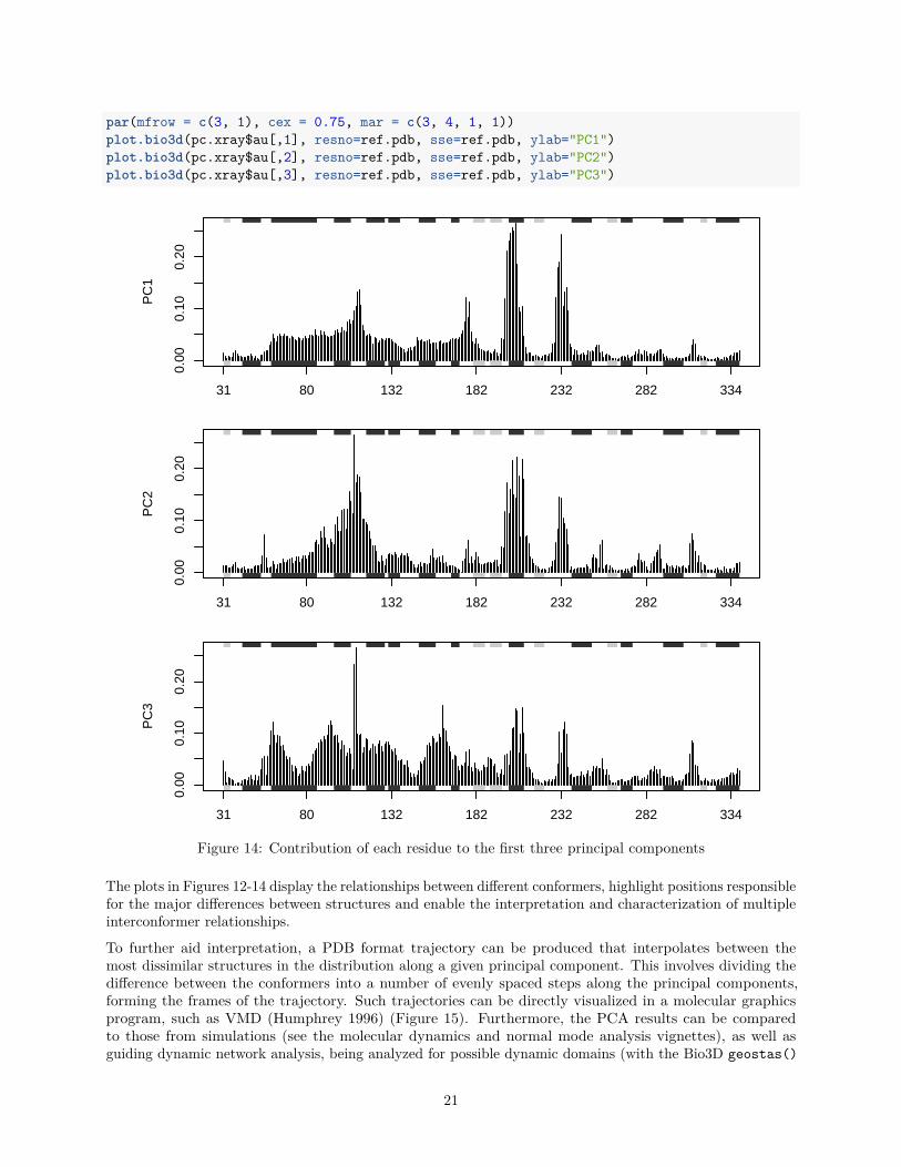
par(mfrow = c(3, 1), cex = 0.75, mar = c(3, 4, 1, 1))plot.bio3d(pc.xray$au[,1], resno=ref.pdb, sse=ref.pdb, ylab="PC1")plot.bio3d(pc.xray$au[,2], resno=ref.pdb, sse=ref.pdb, ylab="PC2")plot.bio3d(pc.xray$au[,3], resno=ref.pdb, sse=ref.pdb, ylab="PC3")

0.00

0.10

0.20

31 80 132 182 232 282 334

Residue

PC

1

0.00

0.10

0.20

31 80 132 182 232 282 334

Residue

PC

2

0.00

0.10

0.20

31 80 132 182 232 282 334

PC

3

Figure 14: Contribution of each residue to the first three principal components

The plots in Figures 12-14 display the relationships between different conformers, highlight positions responsiblefor the major differences between structures and enable the interpretation and characterization of multipleinterconformer relationships.

To further aid interpretation, a PDB format trajectory can be produced that interpolates between themost dissimilar structures in the distribution along a given principal component. This involves dividing thedifference between the conformers into a number of evenly spaced steps along the principal components,forming the frames of the trajectory. Such trajectories can be directly visualized in a molecular graphicsprogram, such as VMD (Humphrey 1996) (Figure 15). Furthermore, the PCA results can be comparedto those from simulations (see the molecular dynamics and normal mode analysis vignettes), as well asguiding dynamic network analysis, being analyzed for possible dynamic domains (with the Bio3D geostas()

21

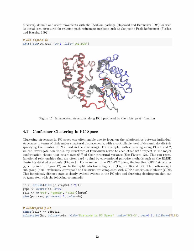
function), domain and shear movements with the DynDom package (Hayward and Berendsen 1998), or usedas initial seed structures for reaction path refinement methods such as Conjugate Peak Refinement (Fischerand Karplus 1992).

# See Figure 15mktrj.pca(pc.xray, pc=1, file="pc1.pdb")

Figure 15: Interpolated structures along PC1 produced by the mktrj.pca() function

4.1 Conformer Clustering in PC Space

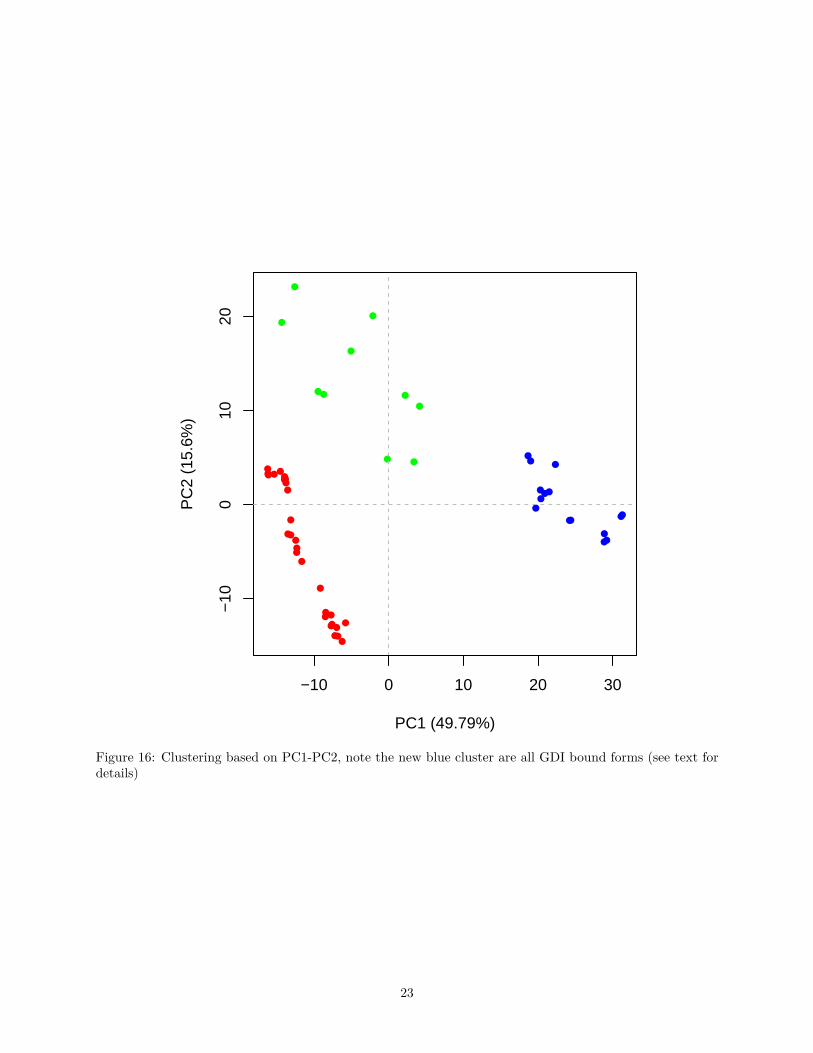
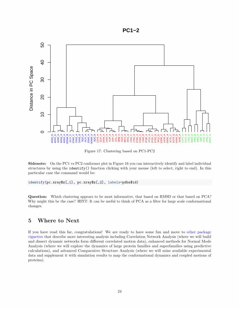
Clustering structures in PC space can often enable one to focus on the relationships between individualstructures in terms of their major structural displacements, with a controllable level of dynamic details (viaspecifying the number of PCs used in the clustering). For example, with clustering along PCs 1 and 2,we can investigate how the X-ray structures of transducin relate to each other with respect to the majorconformation change that covers over 65% of their structural variance (See Figures 12). This can revealfunctional relationships that are often hard to find by conventional pairwise methods such as the RMSDclustering detailed previously (Figure 7). For example in the PC1-PC2 plane, the inactive “GDP” structures(green points in Figure 12) are further split into two sub-groups (Figures 16 and 17). The bottom-rightsub-group (blue) exclusively correspond to the structures complexed with GDP dissociation inhibitor (GDI).This functionaly distinct state is clearly evident evident in the PC plot and clustering dendrogram that canbe generated with the following commands:

hc <- hclust(dist(pc.xray$z[,1:2]))grps <- cutree(hc, h=30)cols <- c("red", "green", "blue")[grps]plot(pc.xray, pc.axes=1:2, col=cols)

# Dendrogram plotnames(cols) <- pdbs$idhclustplot(hc, colors=cols, ylab="Distance in PC Space", main="PC1-2", cex=0.5, fillbox=FALSE)

22

−10 0 10 20 30

−10

010

20

PC1 (49.79%)

PC

2 (1

5.6%

)

Figure 16: Clustering based on PC1-PC2, note the new blue cluster are all GDI bound forms (see text fordetails)

23

PC1−2D

ista

nce

in P

C S

pace

010

2030

4050

4G5Q

_D4G

5O_D

4G5R

_A4G

5Q_A

4G5O

_A3O

NW

_B1K

JY_C

2OM

2_C

2XN

S_A

2XN

S_B

3QI2

_A1K

JY_A

2OM

2_A

3ON

W_A

3QI2

_B1S

VS

_A2Z

JY_A

1SV

K_A

1AS

0_A

1CIP

_A1G

FI_

A1G

IL_A

2IH

B_A

1GIA

_A1B

H2_

A3F

FA_A

1TA

D_C

1TA

D_A

1TN

D_A

1TN

D_C

1TA

D_B

1FQ

K_A

1FQ

J_A

1FQ

K_C

1TN

D_B

1FQ

J_D

2OD

E_C

1AG

R_A

2OD

E_A

3C7K

_C2G

TP

_B1A

GR

_D2V

4Z_A

1GP

2_A

1GG

2_A

1TA

G_A

3QE

0_B

3V00

_B3V

00_A

1GIT

_A1A

S2_

A3V

00_C

1GO

T_A

Figure 17: Clustering based on PC1-PC2

Sidenote: On the PC1 vs PC2 conformer plot in Figure 16 you can interactively identify and label individualstructures by using the identify() function clicking with your mouse (left to select, right to end). In thisparticular case the command would be:

identify(pc.xray$z[,1], pc.xray$z[,2], labels=pdbs$id)

Question: Which clustering appears to be most informative, that based on RMSD or that based on PCA?Why might this be the case? HINT: It can be useful to think of PCA as a filter for large scale conformationalchanges.

5 Where to Next

If you have read this far, congratulations! We are ready to have some fun and move to other packagevignettes that describe more interesting analysis including Correlation Network Analysis (where we will buildand dissect dynamic networks form different correlated motion data), enhanced methods for Normal ModeAnalysis (where we will explore the dynamics of large protein families and superfamilies using predictivecalculations), and advanced Comparative Structure Analysis (where we will mine available experimentaldata and supplement it with simulation results to map the conformational dynamics and coupled motions ofproteins).

24

Document Details

This document is shipped with the Bio3D package in both R and PDF formats. All code can be extractedand automatically executed to generate Figures and/or the PDF with the following commands:

library(rmarkdown)render("Bio3D_pca.Rmd", "all")

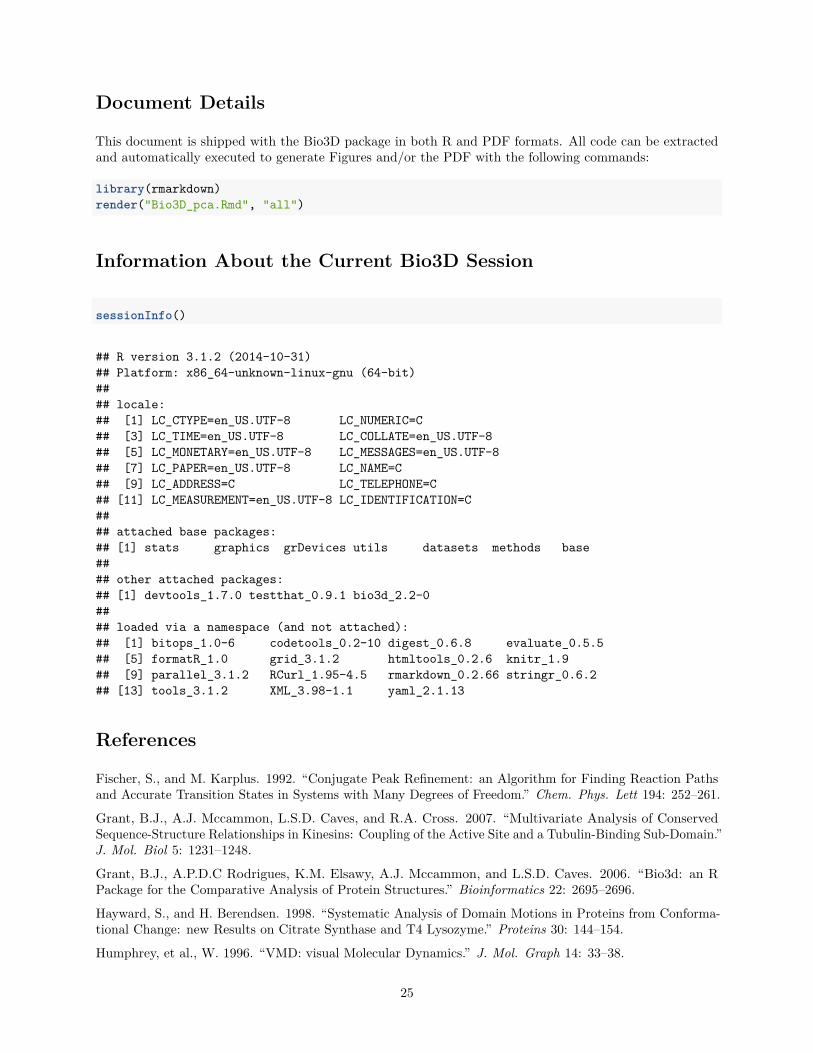
Information About the Current Bio3D Session

sessionInfo()

## R version 3.1.2 (2014-10-31)## Platform: x86_64-unknown-linux-gnu (64-bit)#### locale:## [1] LC_CTYPE=en_US.UTF-8 LC_NUMERIC=C## [3] LC_TIME=en_US.UTF-8 LC_COLLATE=en_US.UTF-8## [5] LC_MONETARY=en_US.UTF-8 LC_MESSAGES=en_US.UTF-8## [7] LC_PAPER=en_US.UTF-8 LC_NAME=C## [9] LC_ADDRESS=C LC_TELEPHONE=C## [11] LC_MEASUREMENT=en_US.UTF-8 LC_IDENTIFICATION=C#### attached base packages:## [1] stats graphics grDevices utils datasets methods base#### other attached packages:## [1] devtools_1.7.0 testthat_0.9.1 bio3d_2.2-0#### loaded via a namespace (and not attached):## [1] bitops_1.0-6 codetools_0.2-10 digest_0.6.8 evaluate_0.5.5## [5] formatR_1.0 grid_3.1.2 htmltools_0.2.6 knitr_1.9## [9] parallel_3.1.2 RCurl_1.95-4.5 rmarkdown_0.2.66 stringr_0.6.2## [13] tools_3.1.2 XML_3.98-1.1 yaml_2.1.13

References

Fischer, S., and M. Karplus. 1992. “Conjugate Peak Refinement: an Algorithm for Finding Reaction Pathsand Accurate Transition States in Systems with Many Degrees of Freedom.” Chem. Phys. Lett 194: 252–261.

Grant, B.J., A.J. Mccammon, L.S.D. Caves, and R.A. Cross. 2007. “Multivariate Analysis of ConservedSequence-Structure Relationships in Kinesins: Coupling of the Active Site and a Tubulin-Binding Sub-Domain.”J. Mol. Biol 5: 1231–1248.

Grant, B.J., A.P.D.C Rodrigues, K.M. Elsawy, A.J. Mccammon, and L.S.D. Caves. 2006. “Bio3d: an RPackage for the Comparative Analysis of Protein Structures.” Bioinformatics 22: 2695–2696.

Hayward, S., and H. Berendsen. 1998. “Systematic Analysis of Domain Motions in Proteins from Conforma-tional Change: new Results on Citrate Synthase and T4 Lysozyme.” Proteins 30: 144–154.

Humphrey, et al., W. 1996. “VMD: visual Molecular Dynamics.” J. Mol. Graph 14: 33–38.

25

Yao, X.Q., and B.J. Grant. 2013. “Domain-Opening and Dynamic Coupling in the Alpha-Subunit ofHeterotrimeric G Proteins.” Biophys. J 105: L08–10.

26