This article was downloaded by: [Memorial University of Newfoundland]On: 02 August 2014, At: 13:52Publisher: Taylor & FrancisInforma Ltd Registered in England and Wales Registered Number: 1072954 Registeredoffice: Mortimer House, 37-41 Mortimer Street, London W1T 3JH, UK

International Journal of GeographicalInformation SciencePublication details, including instructions for authors andsubscription information:http://www.tandfonline.com/loi/tgis20

Comparative performance of logisticregression and survival analysis fordetecting spatial predictors of land-usechangeNinghua Wanga, Daniel G. Brownb, Li Anc, Shuang Yanga & ArikaLigmann-Zielinskad

a Joint Ph.D. Program in Geography, San Diego State Universityand University of California, Santa Barbara, CA, USAb School of Natural Resources and Environment, University ofMichigan, Ann Arbor, MI, USAc Department of Geography, San Diego State University, San Diego,CA, USAd Department of Geography, Michigan State University, EastLansing, MI, USAPublished online: 18 Apr 2013.

To cite this article: Ninghua Wang, Daniel G. Brown, Li An, Shuang Yang & Arika Ligmann-Zielinska(2013) Comparative performance of logistic regression and survival analysis for detecting spatialpredictors of land-use change, International Journal of Geographical Information Science, 27:10,1960-1982, DOI: 10.1080/13658816.2013.779377

To link to this article: http://dx.doi.org/10.1080/13658816.2013.779377

PLEASE SCROLL DOWN FOR ARTICLE

Taylor & Francis makes every effort to ensure the accuracy of all the information (the“Content”) contained in the publications on our platform. However, Taylor & Francis,our agents, and our licensors make no representations or warranties whatsoever as tothe accuracy, completeness, or suitability for any purpose of the Content. Any opinionsand views expressed in this publication are the opinions and views of the authors,and are not the views of or endorsed by Taylor & Francis. The accuracy of the Contentshould not be relied upon and should be independently verified with primary sourcesof information. Taylor and Francis shall not be liable for any losses, actions, claims,proceedings, demands, costs, expenses, damages, and other liabilities whatsoever or

howsoever caused arising directly or indirectly in connection with, in relation to or arisingout of the use of the Content.

This article may be used for research, teaching, and private study purposes. Anysubstantial or systematic reproduction, redistribution, reselling, loan, sub-licensing,systematic supply, or distribution in any form to anyone is expressly forbidden. Terms &Conditions of access and use can be found at http://www.tandfonline.com/page/terms-and-conditions

Dow

nloa

ded

by [

Mem

oria

l Uni

vers

ity o

f N

ewfo

undl

and]

at 1

3:52

02

Aug

ust 2

014

International Journal of Geographical Information Science, 2013Vol. 27, No. 10, 1960–1982, http://dx.doi.org/10.1080/13658816.2013.779377

Comparative performance of logistic regression and survival analysisfor detecting spatial predictors of land-use change

Ninghua Wanga*, Daniel G. Brownb, Li Anc , Shuang Yanga

and Arika Ligmann-Zielinskad

aJoint Ph.D. Program in Geography, San Diego State University and University of California, SantaBarbara, CA, USA; bSchool of Natural Resources and Environment, University of Michigan, AnnArbor, MI, USA; cDepartment of Geography, San Diego State University, San Diego, CA, USA;

dDepartment of Geography, Michigan State University, East Lansing, MI, USA

(Received 11 July 2012; final version received 12 February 2013)

Although survival analysis is known to outperform logistic regression, theoretically andaccording to evidence from other disciplines, little is known about how true this is in sit-uations where the goal is detecting spatial predictors of land change. Furthermore, withthe increasing availability of longitudinal land-change data, evidence is needed on therelative performance of these two different methods in situations with differing levelsof data abundance. To fill this gap, we generated a pseudo land-change data set using anagent-based model of residential development in a virtual landscape. This agent-basedmodel simulated the decisions of homebuyers in choosing residential locations basedon the values of several spatial variables. Pseudo land-change maps, generated by theagent-based model with different weights on these spatial variables, were exposed tostatistical analysis under the logistic and survival approaches. We evaluated how wellthe two approaches could reveal the spatial variables that were used in the agent-basedmodel and compared the performance of the two methods when land-change data werecollected under different sampling frequencies. Our results suggest that survival anal-ysis outperforms logistic regression in detecting the variables that were included inagent decisions, largely because it takes into account time-dependent variables. Also,this research suggests that various properties of land-change processes (like amount ofdeveloped area and access of agents to information) affect the relative performance ofthese statistical approaches aimed at uncovering land-change predictor variables.

Keywords: land-change science; survival analysis; logistic regression; space-timeanalysis; pseudo data set; agent-based model

1. Introduction

Most land-change studies involve two steps: detecting changes in land use or land cover andrelating these changes to some set of predictive or causal factors (Lambin and Geist 2006).Detecting land changes is by no means simple, but advances in the acquisition, processing,and interpretation of remote sensing imagery over the past two decades have made this taskless daunting (Green et al. 1994, Lunetta et al. 2006, Turner et al. 2007). In comparison,however, explaining the observed changes, that is, identifying spatial predictor variablesand their relative contributions, still remains challenging. Too many plausible predictor

*Corresponding author. Email: wangninghua@gmail.com

© 2013 Taylor & Francis

Dow

nloa

ded

by [

Mem

oria

l Uni

vers

ity o

f N

ewfo

undl

and]

at 1

3:52

02

Aug

ust 2

014

International Journal of Geographical Information Science 1961

variables exist, and their effects vary greatly over space, time, and specific context (Geistand Lambin 2002). In recent years, impressive efforts have been made to integrate remotesensing imagery and socioeconomic data (Liverman 1998). These integrated data sets holdgreat promise for identifying predictors of land change, provided appropriate analyticalmethods are applied to them.

Turner et al. (1996) were among the first to suggest using logistic regression for thistask. Because logistic regression is more appropriate for use with categorical outcomes,like land-cover classes, than ordinary least square regression (Lambin 1997, Overmars andVerburg 2005), it soon became widespread in land-change science (Serneels and Lambin2001, Aspinall 2004, Geist and Lambin 2004, Huang et al. 2007, Wyman and Stein 2010).For urban applications, Wu and Yeh (1997) analyzed the impact of land reform policy onChinese urban growth. Their logistic model gave very different estimates (sign and magni-tude) on the same land-change predictor variables, suggesting the structural difference inurban development before and after the reform. Cheng and Masser (2003) continued thiseffort by applying logistic regression, coupled with satellite imagery of 1993 and 2000, andGIS, on Wuhan, a transportation hub in central China. Their model revealed the fading roleof master planning in urban development, with the rise of decentralized decision making.In sum, results of these analyses have contributed considerably to the current knowledgeand understanding of variables associated with various land-change outcomes.

The growing availability of land-change data, often based on satellite imagery, overmultiple time intervals and longer time extents (Mertens and Lambin 2000, Vagen 2006,Zhou et al. 2008), presents a challenge for use of logistic regression. When analyzing longi-tudinal land-change data, logistic regression does not effectively use prior-change temporalinformation. In other words, a change occurring at the beginning of the observation extentis weighed the same as one occurring toward the end of the observation extent. As a result,the significance of a variable’s contribution may be very dependent upon the length ofthe observation extent. To circumvent this challenge, a recent study (Huang et al. 2009)has introduced an exponential smoothing technique on three logistic models that weredeveloped on three consecutive time periods (1984–1992, 1992–1997, and 1997–2002).The smoothing function assigned relatively higher weights on more recent observationsthan older ones. This multi-temporal logistic model effectively predicts land-use change inNew Castle County, Delaware, yet the use of parameters in the smooth function and therelationship to the land-change time remain unclear and are subject to uncertainty.

Survival analysis provides an alternative analytical framework for dealing with longi-tudinal data. Originating in biomedical research, this framework soon gained popularityin many other disciplines where the timing of events is of concern, for example, machinefailure (Cox and Oakes 1984, Mudholkar et al. 1995, Klein and Moeschberger 1997) anddivorce (Smith and Zick 1994, Yashin et al. 1995, Allison 2001, Lee and Wang 2003). Thisframework evaluates causative contributions to the occurrence and timing of the eventof interest. Survival analysis has also found its way to land-change science (Irwin andGeoghegan 2001, An et al. 2011), where it has been demonstrated as a valuable approachto revealing the varying effects of predictor variables on land changes over time.

In theory, survival analysis should outperform logistic regression, as it uses informa-tion more fully. Mathematical analysis has shown that survival analysis is superior when theduration is long and changes are frequent (Green and Symons 1983). This theoretical con-clusion, though it has been verified in fields such as medical science (Green and Symons1983), is not fully tested in application of land-change analysis. Land-change science dif-fers from other fields in its explicit incorporation of spatial and temporal complexitiesin land-change processes. Both survival analysis and logistic regression have strength in

Dow

nloa

ded

by [

Mem

oria

l Uni

vers

ity o

f N

ewfo

undl

and]

at 1

3:52

02

Aug

ust 2

014

1962 N. Wang et al.

modeling individual behaviors, but as land is inherently continuous, how to define the indi-vidual land unit becomes a problem (An and Brown 2008). Two data models are mostcommon in GIS applications: the raster and vector models. The raster model simplifies thespace as a grid of cells, which provides convenience for data handling but short in realisticmapping of natural entities such as mountains and lakes. The vector model, on the otherhand, represents a space consisting of recognizable objects, following their natural shapes,for example, lakeshores or coastlines. Recent application of high resolution remote sens-ing imagery has moved towards reconciling this choice: on the one hand, satellite imagerycan be easily converted to raster data; on the other hand, pixels in high resolution imageare fine enough to capture changes in parcel lots where land-change decisions are usuallymade. In addition to spatial complexity, many characteristics of land, for example, soilfertility and population density, may change over time, which may directly or indirectlyinfluence the direction or rate of land change, adding another layer of temporal complex-ity. Data of higher temporal resolution allow the measure of these dynamic characteristics,but we also need metrics to associate them to land-change events. Survival analysis holdspromise for this aspect because it can accommodate explanatory variables with varyingvalues over time (Allison 2001), which may help to uncover some mechanisms of landchange that could not be revealed by other statistical models.

However, it is important to note that each statistical framework involves a different setof assumptions. Survival analysis is relatively more complex than logistic regression andhas higher requirements on the time resolution of data. As such, the relative performanceof each statistical framework needs to be compared under different circumstances as a wayto improve their use in analyses of land-change processes.

After reviewing literature on logistic regression and survival analysis with consid-erations on model choice, we pursued the following specific research question in thisstudy: How much and under what circumstances does survival analysis perform better thanlogistic regression in detecting predictors of land change?

To answer this question, we evaluated and compared the performances of statisticalmodels estimated under these two frameworks using data on land-change outcomes whoseunderlying mechanisms are well known. The mechanisms were specified in an agent-basedmodel of residential growth. We varied the magnitude of land changes, the level of deter-minism in the agent decisions, the temporal frequency of sampling for the land-changeoutcomes, and the time-varying predictor variables. Statistical model parameters retrievedby the different statistical methods were compared with the known predictor variables usedin the agent-based model to test the accuracy of the different statistical methods underdifferent modeling and sampling conditions.

We limited land changes in the model to those from non-urban use to urban use, whichis mostly irreversible (except over very long time period), as a case study. We acknowledgethat there are other types of land changes that are reversible, for example, between pastureand forest. We concentrated our research on land-use change from non-urban to urban,however, because (1) the non-urban to urban change is common and important in nearly allcountries (Angel et al. 2005) and (2) methodologically, it is fundamental, as a reversibleland change can be decomposed into a chain of short irreversible changes. Nonetheless, theresults of our comparison do not directly apply to reversible land changes. It is important tonote that such changes are particularly complicating, and our survival analysis frameworkwould need to be modified to address irreversible changes, which goes beyond the scopeof this study.

Section 2 reviews these two statistical frameworks and their variants. After impor-tant applied situations are reviewed, the research methods and experimental design are

Dow

nloa

ded

by [

Mem

oria

l Uni

vers

ity o

f N

ewfo

undl

and]

at 1

3:52

02

Aug

ust 2

014

International Journal of Geographical Information Science 1963

described in Sections 3 and 4. Results are presented in Section 5, and Sections 6 and7 discuss implications and conclusions.

2. Regression analysis

Regression analysis is commonly used when measuring correlations between a dependentor response variable and some number of covariates. The distinction between statisticalcorrelation and causation has been elaborated elsewhere (Holland 1986) and must alwaysbe considered when regression is used to evaluate causal relationships. In the context ofland-change science, land changes are widely understood to result from land managers’decisions (Briassoulis 2000, Geist and Lambin 2004, Turner et al. 2007), and factors thatstimulate or constrain land managers’ decisions can be considered as land-change predic-tors. From a pool of potential predictor variables that are informed by theories (Angelsenand Kaimowitz 1999, Irwin and Geoghegan 2001, Walker 2004) and experts’ opinions,those showing significant correlations to land-change events (P-value < 0.05) are oftenidentified as the predictors accounting for land change. Because most predictor vari-ables are spatial in nature, effects of spatial autocorrelation should be taken into account,otherwise P-values can be inflated and false conclusions may arise.

2.1. Logistic regression

Logistic regression was originally used in modeling binary outcomes with a suite ofexplanatory variables, for example, a customer’s purchase decision of a product may relateto product characteristics or demographic, social, and geographic factors associated withthe individual. For land-change science, researchers aim to associate binary land status,for example, changed or not, with a suite of biophysical or socioeconomic variables toexplain land-change processes. Because of the categorical nature of the outcomes, logisticregression was easily adapted for studying predictor variables in land-change applications(Coomes et al. 2000, Cheng and Masser 2003, Huang et al. 2007, 2009, López and Sierra2010, Wyman and Stein 2010). In particular, the maximum likelihood estimation allowsmodelers to evaluate influences from categorical covariates, for example, gender or ethnic-ity (Overmars and Verburg 2005), which has improved the analytical power of regressionin land-change applications.

The most common form of logistic regression uses the logit link function (Equation 1),where Pi is the land-change probability of location i, β0 is the intercept, and X 1 to Xk are kcovariates (i.e., predictors variables) that help explain land status (denoted as Xki for valueat location i), which can be numerical or categorical. Note all variables are italic and samehereafter.

Logit (Pi) = β0 + β1X1i + β2X2i + . . . + βkXki (1)

Despite many advantages, logistic regression suffers an important difficulty for modelingprocesses with multiple time measures. If both land types and covariates change valuesover time, logistic regression has to use either the value at one time or the average overtime, which results in loss of information and reduction in degrees of freedom (An andBrown 2008)

An alternative form of logistic regression, the survey logistic model (‘survey’ modelhereafter) uses piecewise data restructuring (Appendix A). Instead of one probability for

Dow

nloa

ded

by [

Mem

oria

l Uni

vers

ity o

f N

ewfo

undl

and]

at 1

3:52

02

Aug

ust 2

014

1964 N. Wang et al.

each observation or location, which might be thought of as parcels or pixels in the contextof land change, each location can have multiple probabilities, determined by the numberof ‘piecewise’ periods. A location–period probability Pij is defined as the probability thatlocation i experiences land change at period j. This Pij is linked to a period-specific inter-cept β0j and covariates X 1 through Xk of their values at location i and period j (denotedas Xkij in Equation 2). Please note that covariate Xkij may vary over periods. It is calleda survey model because it can group observations from the same unit (e.g., location orhousehold) into a cluster, a technique often used to deal with correlations in survey data(Singer and Willett 2003) and in a similar manner to piecewise longitudinal data. Becausethe survey model uses the latest values of predictor variables of every period, it can handletime-dependent covariates.

Logit (Pij) = β0j + β1X1ij + β2X2ij + . . . + βkXkij (2)

2.2. Survival analysis

Survival analysis is a collection of methods explicitly dealing with the occurrence and tim-ing of events. As a framework specialized for event data, survival analysis is well suited tohandle three types of temporal complexities. First, survival analysis quantifies the poten-tial risk of an event using a ‘hazard’ metric. This hazard metric depends on not only thenumber of events occurred but also their timing. For example, large numbers of events orearly events correspond to higher hazard and vice versa. So events at different time pointsare weighed differently.

Second, survival analysis not only includes samples in which events take place withinthe observation extent, but also samples that experience events of interest before or afterthe observation extent. The latter two cases are called samples censored at left and right,respectively. Sometimes survival analysis can also include interval censored data, wheresamples have events within an interval, but the exact times are unknown.

Third, survival analysis allows for covariates with time-varying values, that is, time-dependent covariates. For example, the population density of an area may increase anddecrease over time. Survival analysis uses the updated population density to estimate thehazard of a location in that area.

In sum, these features allow survival analysis to use more temporal information, min-imizing uncertainties in the estimation process. As such, survival analysis has gainedattention in land-change science (Irwin and Bockstael 2004, Iovanna and Vance 2007, Anand Brown 2008, An et al. 2011). It is worth noting, however, that survival analysis ispredominantly applied to study death or other irreversible processes. Although many landchanges are irreversible, some are reversible, which may present limits to the applicabilityof survival analysis.

Interpretation of survival models is similar to logistic regression, for example, the eval-uation of significance of covariates, except (1) the dependent variable is hazard instead ofprobability and (2) intercept h0(t)can be a function of time (Equation 3).

Log hi(t) = Log h0(t) + β1X1i(t) + β2X2i(t) + . . . + βkXki(t) (3)

where hi(t) is the hazard of location i at time t, h0(t) is the baseline hazard shared by alllocations, and Xk is the kth covariate.

Dow

nloa

ded

by [

Mem

oria

l Uni

vers

ity o

f N

ewfo

undl

and]

at 1

3:52

02

Aug

ust 2

014

International Journal of Geographical Information Science 1965

In survival analysis, the form of the intercept function Log h0(t) is usually difficultto specify. There are generally two ways to solve this problem: parametrically using apiecewise exponential model (Allison 2001) and semi-parametrically using the Cox pro-portional hazard (PH) model (Cox 1972). The piecewise exponential model (‘piecewise’model hereafter) breaks the entire study time extent into a certain number of periods andapproximates the intercept in period j to a constant β0j (Equation 4). When periods are suf-ficiently short, this approximation is quite reasonable. The Cox PH model (‘Cox’ modelhereafter), in comparison, circumvents the task of specifying the intercept function bydividing hazards of early events over hazards of later events. Because all hazards share thesame intercept function, it cancels out. As such, coefficients β1 to βk are directly estimatedfrom hazard ratios. For more details, please refer to Allison (2001).

Log hi(t) = β0j + β1X1ij + β2X2ij + . . . + βkXkij (4)

where j = 1,2,. . .J , J is the number of periods. Xkij is the value of nth predictor at locationi in period j (note that Xkij may have different values over periods). hi(t) is the hazard oflocation i at time t.

In sum, two analytical frameworks in four variants were examined (Table 1). Table 1also lists the assumptions, data distributions, and calibration algorithms of these statisticalmethods.

3. Model selection

As in any statistical analysis, selection of model form is critical in land-change science(Agarwal et al. 2002, Parker et al. 2003, Lambin and Geist 2006), yet systematic explo-rations of the behaviors and suitabilities of different model forms have not been doneadequately (Turner et al. 2001). Models are instruments of inquiry for specific purposes.So the appropriateness of a model is first evaluated by whether it serves the research pur-pose, in our case to identify land-change predictors. After the purpose is clear, we need to

Table 1. Summary of statistical models examined in this study.

Logistic Survival

Model Logit Survey Cox Piecewise

Response variabledistribution

Binary or discrete Discrete and/or continuous

Link function Logit function Hazard functionIndependent variable

distributionContinuous and

categority, okay onnon-normality

Continuous and categority, okay onnon-normality

Time-varying independentvariable?

No Yes Yes Yes

Intercept Constant Piecewise Canceled PiecewiseAssumption asymptote asymptote PH assumption constant intervalCalibration algorithm MLE MLE P-MLE MLEDiagnostic methods ROC, deviance,

goodness-of-fit,generalized R2

Generalized R2, schoenfeld residual,deviance, martingale residual

Dow

nloa

ded

by [

Mem

oria

l Uni

vers

ity o

f N

ewfo

undl

and]

at 1

3:52

02

Aug

ust 2

014

1966 N. Wang et al.

consider a number of factors, such as assumptions, temporal data completeness, and levelsof complexity (Allison 2001, Harrell 2001).

First, all models make assumptions to provide simplified representations of the realworld. Statistical models function properly only when the assumptions are good approx-imations of the situations represented in the data. The Cox model, for example, assumesthat covariates (i.e., predictor variables) exert constant influences on hazards over time,a.k.a. the PH assumption (Singer and Willett 2003). The piecewise model assumes con-stant effects within each time period. These assumptions may be violated in the case ofrapid land-change processes. For example, in a competitive land market, land desirability(or hazard) would increase over time as land resource is exhausted. In that way, covariates’effects on land desirability inflate rapidly with time, violating the PH assumption.

Second, different models differ in whether they handle time discretely or continuously.However, as the discrete time intervals shrink, it is not always clear when to switch toa continuous-time model. As land-change science shifts to interest in and availability offine temporal resolution data, we need to know when survival analysis will produce betterresults.

Third, land changes occur within complex socio-ecological systems. Modelers have tostrike a balance between taking adequate account of system complexity on one the handand seeking an explicable, parsimonious model on the other. Agarwal et al. (2002) outlinedthree dimensions of complexity for socio-ecological systems: spatial, temporal, and humandecision-making. Specific modeling approaches are often strong at modeling complexityin one dimension, but weak in others. So model selection depends upon the dimension(s)of complexity that modelers intend to address.

4. Methods

We used a diverse set of land-change conditions to test alternative statistical models.We adopted a novel computational approach as follows (Figure 1). With a specific set ofvariables and parameters, we (1) simulated a land-change process, (2) sampled the data thatresulted from that process spatially and temporally following specific rules, (3) exposed thesampled data to statistical models of interest, and (4) evaluated those models by compar-ing their coefficients to the actual parameters we programmed for a given simulation. Thisevaluation procedure was repeated 1000 times over different model variables and parametervalues, both selected by the Monte Carlo technique.

4.1. Simulation approach

To evaluate the performance of statistical models under a range of conditions, we sim-ulated those conditions by using a Monte Carlo technique to generate results from anagent-based model of LUCC under a sample of parameter combinations. We generateddata through simulation, as opposed to empirically, for three reasons. First, a simulateddata set minimizes uncertainties in model assessment, which often arise when assessingstatistical methods with real data because it is possible only to hypothesize about whatare the underlying mechanisms by using various theories, experts’ opinions, and statisticalevaluation methods. It is not possible to know for certain, or to manipulate with experi-mental control, the underlying mechanisms generating a real-world data set. However, byusing a simulation approach, the underlying mechanisms, variables, and parameters arecompletely known and the ability of statistical models to recover them can be accuratelyassessed (Hirzel et al. 2001).

Dow

nloa

ded

by [

Mem

oria

l Uni

vers

ity o

f N

ewfo

undl

and]

at 1

3:52

02

Aug

ust 2

014

International Journal of Geographical Information Science 1967

Figure 1. Steps involved in evaluation of statistical results in the context of each land-changeprocess.

Second, comparing methods using empirical case study data, as has been done in pre-vious work (Malanson 2005, An and Brown 2008, Pontius et al. 2008), limits the appliedsituations under which the methods can be explored. Different land-change processesinvolve different predictor variables (An and Brown 2008, Rindfuss et al. 2008, An et al.2011), changing at different speeds (Lambin and Geist 2006) and involving different levelsof information access by land managers and users (Manson 2006). These factors lead todiverse land-change pathways. Constructing an empirical data set that represents a widerange of pathways is very difficult, but relatively easy for a simulation data set where alter-ation of the simulation program’s initial parameters produces a diverse set of pathways(Clarke et al. 2007, Rindfuss et al. 2007). As such, we can map the relative performanceof each statistical technique across applied situations.

Third, the simulation approach enables full control of data production and ensures datacompleteness (Neel et al. 2004, Epperson et al. 2010). Data completeness refers to theresolution and extent of data coverage. It is a key factor in model selection (Harrell 2001),and it is often limited spatially and temporally in real data sets. To study the sensitivity ofstatistical models to these kinds of limits, we test models on data sets sampled at differentfrequencies.

There is a risk that virtual land-change processes generated by a certain simulation pro-gram may lack generality, limiting range of conditions under which conclusions about theefficacy of statistical methods may apply. In this study, we replicated all our experimentsusing a second simulation program (Ligmann-Zielinska and Sun 2010). This agent-basedmodeling (ABM) program is a simplified implementation of a residential developmentprocess, focusing on site suitability assessment and investment decisions. Because of

Dow

nloa

ded

by [

Mem

oria

l Uni

vers

ity o

f N

ewfo

undl

and]

at 1

3:52

02

Aug

ust 2

014

1968 N. Wang et al.

space limit, replication details and results are presented in Appendix B and in onlinesupplementary document.

4.2. Simulation model

Developed by the Spatial Land Use Change and Ecological Effects (SLUCE)project (http://www.cscs.umich.edu/sluce/ ), the SOME (SLUCE’s Original Model forExperimentation) model was selected for our study because of its parsimonious represen-tation of land dynamics using ABM techniques (Brown et al. 2005). ABM is a categoryof computational models that directly simulates the behaviors of individual agents (Parkeret al. 2003), where agents act autonomously in the course of simulation, following rulesdesigned by modelers.

SOME consists of three primary parts: a virtual landscape, a group of agents repre-senting homebuyers, and their behavior rules. The land market is simplified by consideringdemand only, while the supply of homes always meets demand. The landscape in SOMEis a lattice of cells of equal size. Each homebuyer acquires one and only one cell, which isthen converted to residence, resulting in land-use change. The global land-use change pat-tern is a consequence of location decisions by a sequence of homebuyers. Homebuyersevaluate cells based on a utility function ux,y(t) (Equation 5), where x and y are coor-dinates of a given cell and select from a pool of candidate cells the one with highestutility.

ux,y(t) = (AQx,y(t))αAQ × (1/SCx,y(t))αSC × (1/Wx,y)αW (5)

It is not possible to include all land-change driving forces in any given simulation. Forsimplicity, we included three potential variables in utility function, aesthetic quality (AQ),distance to service center (SC), and distance to water (W ). The influences by these vari-ables are adjusted by αAQ, αSC , and αW , whose values we alternate between 0 and 1 forthese experiments. We assumed a lake on the left border of the landscape, so W is theEuclidean distance from the border. SC is the Euclidean distance to the nearest servicecenter. Initially, we place a service facility at the center of the landscape. As the simula-tion continues, a new service facility is added to the landscape for each additional set of100 homebuyers; the location of the service facility is near the location chosen by the lasthomebuyer. This process continues until a certain proportion of the landscape is occupiedor a specified number of time steps has passed. The AQ value is derived from a predeter-mined 121 by 121 random map of AQ with positive spatial autocorrelation (Figure 2). Thispositively autocorrelated map was generated by (1) creating 100 random points, each witha random value, (2) applying a kriging interpolation on those points to smooth the surface,and (3) dissecting a 121 by 121 grid from the virtual terrain. Developments (residents andservice centers) at nearby locations, defined by a 3 × 3 window around each cell, nega-tively affect the AQ value of that cell by a constant fraction each time a new developmentis created. For more information about SOME, please refer to An et al. (2005) and Brownet al. (2005).

We chose AQ, SC, and W for the following reasons. First, they represent biophysicaland socioeconomic variables, two general categories most common in land-change pro-cesses. Second, they possess a wide range of time variability: W has a fixed value overtime, with development, AQ, and SC decrease over time. Predictor variables from the realworld would mostly fall into this range. Figure 3a, b, and c shows how land-change patternsare affected by AQ, SC, and W , respectively.

Dow

nloa

ded

by [

Mem

oria

l Uni

vers

ity o

f N

ewfo

undl

and]

at 1

3:52

02

Aug

ust 2

014

International Journal of Geographical Information Science 1969

Figure 2. Virtual landscape of aesthetic quality considering spatial autocorrelation.

Figure 3. Land-change patterns created when agents consider only (a) aesthetic quality (AQ), (b)distance to service center (SC) or (c) distance to water (W ) in their utility calculation.

4.3. Experimental procedures

To learn the relative performance of statistical models, we tested them each for a widerange of land-change conditions. Theory and applications in other domains show that sur-vival analysis outperforms logistic regression, so an experiment over all conditions shouldreproduce this finding. Further, an examination of variations between conditions wouldinform us of the relative performance of each method in different application situations.In particular, land-change conditions are simulated as follows.

First, we ran the model with each predictor turned on (α = 1) and off (α = 0), respec-tively, resulting in eight conditions, for example, all on or off, one on and the other two off,or one off and the other two on. This approach is to simulate the challenge in identifyingeffective variables from a pool of potential ones (Hersperger and Bürgi 2009).

In addition, we selected two parameters out of a dozen from SOME and swept allvalues over their ranges. The first parameter, called numresidents, controls the amount ofland change that the model produces by determining how many residents enter. For everysimulation step, the same number of residents (numresidents) enters the landscape. When

Dow

nloa

ded

by [

Mem

oria

l Uni

vers

ity o

f N

ewfo

undl

and]

at 1

3:52

02

Aug

ust 2

014

1970 N. Wang et al.

numresidents is high, more land is developed at every step, so there will be more changesacross space and over time. The second parameter, called numtests, controls the number ofcandidate cells that a homebuyer evaluates when searching the landscape. High numtestsimplies high level of access to information about available land. Candidate cells are drawnrandomly, in attempt to represent realistic conditions of personal preference, institutions,and other constraints on access to land information. High numtests reduces process ran-domness, resulting in more deterministic spatial patterns and temporal dynamics of landchange. On the contrary, low numtests results in stochastic development patterns in spaceand time. We acknowledge that in real world, there may be more land-change pathwaysthat cannot be controlled by these two parameters. However, we would like to choose thembecause (1) they determine the quantity and spatial distribution of land change (Figure 4)and (2) they affect the validity of some statistical assumptions (e.g., PH assumption in theCox model) when their values go to extremes.

We used the Monte Carlo technique to produce land-change conditions from a largenumber of possibilities (Table 2). Because numtests and numresidents are continuous mea-sures, we grouped their values for analysis into a priori ranges, determined through asensitivity analysis, and uniformly sampled within each range (Figure 4). We sampled1000 specific land-change conditions, from the full set of possible parameter combinations,on our workstation (Dell Precision T5400 Intel Xeon 3.16 GHz Qual-core 16G memory).

4.4. Space–time sampling

Mapped results from the above land-change simulations were sampled spatially and tem-porally. A combined sampling scheme of systematic and random sampling (Cheng andMasser 2003, Luo and Wei 2009) was adopted to minimize autocorrelation while main-taining the representativeness of samples. We tested the residuals of regression analysisand found that as the sample size decreased from 20% to 5%, Moran’s I decreased from0.23 (z-score = 4.02, positive autocorrelation) to 0.027 (z-score = 1.46, no autocorre-lation). Also, 5% sampling at different time points maintained a Moran’s I of less than0.1, with z-score <1.96. As such, we kept sampling at 5% by the given sampling schemethroughout the research. All attributes of those cells were saved: their development status,values of aesthetic quality, distance to service center, and distance to water at each specifictime point.

To explore the effects of temporal resolution for sampling, five different sampling fre-quencies (expressed in number of steps between two consecutive samples) were used: 10,20, 30, 40, and 50, given 200 time steps in total. Though we were able to collect simu-lation data at each time step, it would make more sense to test model performance whendata are collected less frequently, for example, every 10 steps up to every 50 steps. In thereal world, it is often difficult to collect historical data of land use at a yearly basis, so thetest of models at coarser temporal resolutions holds more importance. All models wereassessed at highest frequency first (i.e., every 10 steps), and the effect of frequency on theperformance of the statistical analyses was assessed as we sampled less frequently.

Sampled data were used as input to the statistical models. With the exception of thelogit model, which only needed data at two time points, usually the start and the end, allstatistical analyses used data at every sampled time point.

4.5. Implementation of statistical models

Our statistical models were implemented in SAS (http://www.sas.com/ ). To avoid softwarebias, analyses on the same data sets were replicated in R (http://www.r-project.org/ ) and

Dow

nloa

ded

by [

Mem

oria

l Uni

vers

ity o

f N

ewfo

undl

and]

at 1

3:52

02

Aug

ust 2

014

International Journal of Geographical Information Science 1971

Figure 4. Illustration of nine distinctive parameter combinations by sweeping simulation param-eters numtests and numresidents, with SC as the only driver. We adopted Monte Carlo techniqueto evenly explore combination (a) through (i). (a) low numtests and low numresidents; (b) mediumnumtests and low numresidents; (c) high numtests and low numresidents; (d) medium numtests andlow numresidents; (e) medium numtests and medium numresidents; (f) medium numtests and highnumresidents; (g) high numtests and low numresidents; (h) high numtests and medium numresidents;(i) high numtests and high numresidents.

MATLAB (http://www.mathworks.com/ ). All statistical models were specified in theiroriginal forms, that is, no interaction terms introduced (Appendix C), which is consistentwith the utility function (Equation 5).

4.6. Evaluation

Finally, the accuracy of the resulting statistical models was assessed by comparing theresultant coefficients to the parameters in the agent-based models. We set up two standards

Dow

nloa

ded

by [

Mem

oria

l Uni

vers

ity o

f N

ewfo

undl

and]

at 1

3:52

02

Aug

ust 2

014

1972 N. Wang et al.

Table 2. Parameter values used in sampling land-change conditions for simulation.These values are uniformly sampled in 1000 Monte Carlo experiments.

Parameter Possible values

AQ on, offSC on, offW on, offNumtests (information access) low ( <0.1% off landscape)

medium ( >0.1%, but<1%) high ( >1%)

Numresidents (development percentage) low ( <10% of landscape)medium ( >10%, but<75%) high ( >75%)

for assessing the statistical models. A model was considered partially successful if thecontribution of one potential predictor variable was correctly detected, that is, it shows sta-tistical significance (P-value < 0.05) when the corresponding factor is turned ‘on’ (α inEquation 5 equals ‘1’) or it shows statistical insignificance (P-value > 0.05) when the cor-responding factor is turned ‘off’ (α equals ‘0’). A model was considered fully successful ifall predictor variables were correctly detected. The rates of partial and full success usuallyturned out to be the same in our experiments, so we report only the full success rate, exceptfor the section on time-dependent variables and in Figure 6, where the partial success ratewas used.

5. Result

5.1. Overall performance

Of the 1000 Monte Carlo experiments, the piecewise model achieved the highest (full)success rate (Figure 5). The Cox model, a variant of survival analysis, received the secondhighest success rate. No logistic model had a success rate above 40%.

Figure 5. Overall full success rates of the different statistical models, after 1000 Monte Carloexperiments.

Dow

nloa

ded

by [

Mem

oria

l Uni

vers

ity o

f N

ewfo

undl

and]

at 1

3:52

02

Aug

ust 2

014

International Journal of Geographical Information Science 1973

Figure 6. The relative partial success rates for different models on the time-independent variable(W ) and the time-dependent variables (AQ and SC).

Besides the success rate, logistic regressions were diagnosed by statistical indicators,including over-dispersion, lack of fit, and Receiver Operating Characteristic (ROC) curve.No over-dispersion was found (P-value = 0.99 for deviance rejected the over-dispersionhypothesis) in the response variable, and logistic models showed good fit to data from testson ROC (average = 0.92, SD = 0.16) and Hosmer and Lemeshow goodness-of-fit (P-value= 0.91, where goodness-of-fit is rejected when P-value < 0.05). Still, different statisticalindicators could reveal different aspects of the model, and the success rate proposed by uspresented some new information.

This Monte Carlo result helps us understand how survival analysis performs relativeto logistic regression. However, to understand the application situations over which eachstatistical model is effective, we need to further explore the results of 1000 experiments.

5.2. Time-dependent and -independent variables

Different land-change predictors show different levels of temporal variability, that is, somepredictors (e.g., distance to water) have fixed values over time, while others (e.g., distanceto service center and aesthetic quality) change values with land developments. In general,it is more difficult to measure the effects of time-dependent predictors. However, it is com-monplace to have time-dependent predictors in land-change process models, for example,population density.

Using the partial success rates, we evaluated every statistical model for success indetecting the importance of each variable (Figure 6). All statistical models performed betterin detecting the time-independent variable, W , than in detecting time-dependent variables,SC and AQ (except in the Cox model, AQ has higher success rate). The success rate forW ranges from a high value of 94%, for the piecewise model, to a low value of 82%, forthe logit model. Time-dependent variables were more difficult to detect with success rateranging from 88% to 54%.

While success rates for detecting the time-independent variables and time-dependentvariables were different among all statistical models, the differences were larger for the

Dow

nloa

ded

by [

Mem

oria

l Uni

vers

ity o

f N

ewfo

undl

and]

at 1

3:52

02

Aug

ust 2

014

1974 N. Wang et al.

logistic models. The survey model had the largest difference (41%) and the logit modelthe second largest (30%). In contrast, the differences for two survival models were muchlower (12% for the Cox model and 9% for the piecewise model). This indicates a greaterconsistency in model performance for the survival models compared to the logistic models.

5.3. Development percentage and information access

Monte Carlo experiments over nine different combinations of values of the two continu-ous parameters, numresidents and numtests in Figure 4, revealed considerable variability infull success rates (Figure 7). The piecewise model outperformed other models for almostevery combination, except in combination e, where the logit model performed equally well.Also, the piecewise model did not show much variability across different parameter combi-nations, indicating that it is a robust model for dealing with various land-change situations.

The logit model performed well when the development percentage was at medium level(e.g., combinations b, e, and h in Figure 7), but worse when the development percent-age was low or high. This finding is consistent with literature (Cramer 1999, King andZeng 2001), in which extreme binary ratios, that is, data dominated by 1’s or 0’s, deterio-rates model performance. In the context of land change, situations such as rare changes orubiquitous changes are not appropriate for the logit model.

In theory, high information access would pose a challenge to the PH assumption ofthe Cox model, since high information access leads to more competition for the same landparcels and, therefore, scarce land resources. As such, the effects of covariates on landattractiveness would appear to increase over time, which challenges the PH assumptionthat covariates hold constant effects over time. This challenge, however, does not produceserious bias according to our results. The Cox model maintains high success rate (>65%)in situations with high information access, unless the development percentage is also high(success rate = 55% at combination i).

5.4. Sampling frequency

Sampling frequency had an impact on the Cox, piecewise, and survey model and no impacton the logit model, which only uses data at two times (one at the beginning of the run andone at the end). Although the sampling frequency has a direct effect on the piecewise modeland the survey models, by determining into how many ‘pieces’ the longitudinal data willbe segmented, the effect on the Cox model is less obvious, in that it affects the calculationof hazard. Nonetheless, the general effect on the success rate is the same: because at higher

Figure 7. Full success rates of statistical models for each combination of development percentage(numresidents) and information access (numtests).

Dow

nloa

ded

by [

Mem

oria

l Uni

vers

ity o

f N

ewfo

undl

and]

at 1

3:52

02

Aug

ust 2

014

International Journal of Geographical Information Science 1975

Figure 8. The impacts of sampling frequency on full success rates.

frequencies, more temporal information is retained, statistical models are more likely todetect the corresponding land-change variables, whereas at lower frequencies they are lesslikely to detect variables (Figure 8). All models except the logit model performed betterwhen the sampling frequency was higher, that is, more samples over time, because moreinformation is used.

6. Discussion

This study used simulation data to investigate the performance of survival analysis andlogistic regression in different applied situations. This simulation approach provided us theconvenience to preset predictors of land change and test if they are reflected in statisticalresults. Also, it could span a wide range of land-change conditions, making it possibleto evaluate statistical methods in different situations and in the future to explore theirapplication domains.

In detecting spatial predictors of land change, our experiments with simulated datahave shown that survival analysis consistently outperformed logistic regression. This find-ing conforms to theory, corroborating the usefulness of our simulation approach. Amongmany survival models, the piecewise model has better revealed the role of spatial predictorvariables. Full use of information and less violation to model assumptions may explainwhy the piecewise model performed the best. Among logistic models, the logit model wasbetter than the survey model, which may be explained by the severe imbalance between ‘0’and ‘1’ in piecewise data (see below).

More importantly, we explored the relative performance of the two methods in dif-ferent application situations regarding temporal characteristics of effective predictors, thepercentage of development, the level of information access, and data completeness. Allthese factors could impose challenges to the task of detecting predictor variables, limitingthe application situations of statistical models.

Dow

nloa

ded

by [

Mem

oria

l Uni

vers

ity o

f N

ewfo

undl

and]

at 1

3:52

02

Aug

ust 2

014

1976 N. Wang et al.

One important temporal complexity in land-change science is the changing characteris-tics of some environmental factors over time or time-dependent variables. Survival modelsare advantageous in detecting time-dependent variables, that is, where the value of a pre-dictor variable changes over time (Allison 2001, An and Brown 2008). Survival modelsassociate changes in land hazards to changing values of time-dependent variables, so esti-mate accurately the effects of these variables. Logistic models overlook time variabilityof variables, so when time-dependent variables are present, they are prone to erroneousestimates.

Logistic models did not perform well when the amount of development was very low(<10%) or very high (>75%). In fact, logistic models require balanced binary values,that is, similar numbers of ‘0’ and ‘1’ (Cramer 1999, King and Zeng 2001, Heinze andSchemper 2002, Fletcher et al. 2005). This finding has important implications for land-change studies. Many land-change cases are either very slow, for example, establishedurban areas in developed countries, or very fast, for example, deforestation in frontiers.These situations may lead to unbalanced land outcomes that pose challenges to logisticmodels. Cheng and Masser (2003) and Huang et al. (2009) indirectly solved this unbal-anced data issue by applying two different sampling schemes to converted and unconvertedland separately. Nonetheless, when the total amount of converted or unconverted land issmall, sampling a fraction of land, for example, 5%, will result in a very small sample size.As such, it might be difficult to fulfill sample size requirement.

Land development leads to land resource depletion. However, according to the mecha-nisms in the SOME model, when information access is high or, in other words, when thecandidate pool is large, lands with high covariate values are always included in the can-didate pool and quickly depleted. As a result, lands with lower covariate values becomecompetitive for later time since high value lands are gone. In other words, the same covari-ate has increased impact on the hazard of being developed (Figure 9). This outcomeessentially violates the PH assumption that covariates exert constant effect to the hazardover time. While in theory this might be the case, in experiments we found that for Coxmodel, moderate violation of this assumption did not have detectable effects on our results.

Figure 9. Land resource depletion over time causes inflated effect of covariates on hazard, illus-trated by W as the major factor. Note that low W is preferred (closer to water) but over time lands farfrom water are developed.

Dow

nloa

ded

by [

Mem

oria

l Uni

vers

ity o

f N

ewfo

undl

and]

at 1

3:52

02

Aug

ust 2

014

International Journal of Geographical Information Science 1977

The performance of survival models hinges on sampling frequency. High frequencyimproves performance because more dynamic information is captured. Performance of thelogit model, in contrast, is independent of sampling frequency, because it includes only twostates of land (e.g., the beginning and final states) in its analysis. In general, survival modelsare recommended unless temporal information is limited; when this limit exists, the logitmodel should be considered with concerns about its other conditions (e.g., balance between‘0’s and ‘1’s).

For the purposes of evaluating alternative statistical models, the simulation approachseems to be very useful. It complements conventional applications of statistical modelsto empirical data in at least two respects. First, by simulating land-change processes, thevariables and parameters that are used to generate a given pattern are known completely,and statistical modeling results can be compared to those known characteristics. Second, arich and diverse set of land-change processes can be generated, as opposed to one or a fewthat might be contained in an empirical setting, providing us insights into the usefulnessof alternative statistical models under a diverse range of conditions. Although the near-transparent quality of simulated data has been often used in other domains to quantifymodeling results (Foss et al. 2003, Burton et al. 2006), it is less common in geography(Hirzel et al. 2001) and has never been applied to assess the ability of statistical models todetect predictor variables in land-change applications.

There is a risk that virtual processes do not reflect the wide range of possible underly-ing processes very well, introducing limits to the generality of the results. In this study, wereduced this risk by several means: (1) to validate our findings, we used another simulationprogram, which was independently developed based on different assumptions and con-ceptualizations, and the match of results corroborates our findings (Appendix B); (2) theMonte Carlo technique we employed randomly sampled the parameter space of our simu-lation program, allowing comprehensive assessment of various situations under which ourland-change model might function; and (3) we tested all possible combinations of predictorvariables, for example, the eight cases in our study. This mimicked the situation in whichwe are unaware of the true predictor values and have to make decisions from a pool ofpotential predictors.

This research investigated the relative performance of survival analysis and logisticregression using data from non-urban to urban land, a common land-change type that hasbeen well studied (Lambin 1997, Cheng and Masser 2003, Huang et al. 2009). It mayalso represent a wide range of land-change types that are irreversible or unidirectional.However, some conversions are reversible, for example, two-way changes between tilledand untilled agricultural land or between pasture and forest. These reversible land changes,or multi-event (on the same land unit) processes, certainly complicate the application ofsurvival analysis, and these complications may present situations in which survival anal-ysis is less suitable for application. It is possible to segment a reversible land-change intoa series of irreversible changes, and variants of survival analysis have been reported to beable to handle multi-event processes (Allison 2001, Andersen and Keiding 2002). Futurestudies will need to test survival analysis methods on reversible land changes. If the simula-tion approach is used, the selected simulation model needs to reflect this type of multi-eventprocess accordingly.

Several new directions will be explored in the future. First, this simulation study shouldbe linked to empirical studies. We are in the process of collecting satellite imagery andsocioeconomic data in a time series and experiment with how the increase in temporalresolution of data affects statistical results. Second, we could more thoroughly appraise sta-tistical models using other non P-value indicators, such as coefficients of covariates. Third,

Dow

nloa

ded

by [

Mem

oria

l Uni

vers

ity o

f N

ewfo

undl

and]

at 1

3:52

02

Aug

ust 2

014

1978 N. Wang et al.

survival models should be integrated with land-change analysis more tightly in terms ofmethod and conceptualization. Our experimentation reveals the practical aspects of sur-vival analysis in probing simulated dynamic land-change systems. Since survival analysisoutperforms other analytical techniques when temporal variability is present (e.g., dynamicfactors), it can be utilized in studies where disturbances, abrupt events, and policy inter-ventions are introduced into the system. Not only do such disruptions change the dynamicsof land patterns, but they may also affect the predictors themselves.

7. Conclusion

This study confirms the theoretical speculation that survival models generally perform bet-ter than logistic models using simulation-based land-change data. This may arise fromsurvival models’ more effective use of temporal information. We present our findings in thehope that more research would be devoted to this type of models in land-change analysis.

Furthermore, this study provides insights into the relative performance of survival mod-els and logistic models, an important step towards better defining application domains ofthese methods. It appears that survival models perform better in detecting time-dependentvariables and are robust to handle very fast/slow land-change processes and varying lev-els of information access. Logistic models are not recommended when very fast or slowland-change processes give rise to highly unbalanced land outcomes (i.e., nearly all devel-oped or undeveloped) or when information access is extremely high or low. The only timelogistic regression might be recommended is when samples in time are very sparse.

The simulation approach is useful when assessing the inferential power of statisti-cal models in land-change studies. One advantage that cannot be otherwise obtained isits endowment of a land-change researcher’s better control of experiment processes (thusless ‘noise’ or unknown processes), allowing for potentially more accurate assessment ofdifferent statistical models when applied in different land-change situations.

AcknowledgmentsThis research was funded by National Science Foundation: the Biocomplexity in the EnvironmentProgram (BCS-0119804) and SLUCE II project (GEO-0814542), the Partnership for InternationalResearch and Education (PIRE; OISE-0729709) Program, and the Dynamics of Coupled Natural andHuman (CNH) Systems (DEB-1212183) Program. It was also supported by 2) SDSU UGP Projectunder the title ‘Sampling at What Scales? A Computational Simulation Approach’. The authors thankthree anonymous reviewers for their valuable comments and suggestions.

ReferencesAgarwal, C., et al., 2002. A review and assessment of land-use change models: dynamics of space,

time, and human choice. USA: Forest Service. Northeastern Research Station.Allison, P., 2001. Survival analysis using the SAS system: a practical guide. Cary, NC: SAS

Publishing.An, L. and Brown, D., 2008. Survival analysis in land change science: integrating with giscience

to address temporal complexities. Annals of the Association of American Geographers, 98,323–344.

An, L., et al., 2005. What statistical models help to detect land-change mechanisms?GeoComputation 2005, Ann Arbor, Michigan.

An, L., et al., 2011. Variations in development of exurban residential landscapes: timing, location,and driving forces. Journal of Land Use Science, 6, 13–32.

Andersen, P.K. and Keiding, N., 2002. Multi-state models for event history analysis. StatisticalMethods in Medical Research, 11, 91–115.

Dow

nloa

ded

by [

Mem

oria

l Uni

vers

ity o

f N

ewfo

undl

and]

at 1

3:52

02

Aug

ust 2

014

International Journal of Geographical Information Science 1979

Angel, S., et al., 2005. The dynamics of global urban expansion. Transport and Urban DevelopmentDepartment, The World Bank, Washington D.C., 1, 1–11.

Angelsen, A. and Kaimowitz, D., 1999. Rethinking the causes of deforestation: lessons fromeconomic models. The World Bank Research Observer, 14, 73–98.

Aspinall, R., 2004. Modelling land use change with generalized linear models–a multi-model anal-ysis of change between 1860 and 2000 in Gallatin Valley, Montana. Journal of EnvironmentalManagement, 72, 91–103.

Briassoulis, H., 2000. Analysis of land use change: theoretical and modeling approaches. Availablefrom: http://www.rri.wvu.edu/WebBook/Briassoulis/contents.htm [Accessed 21 January 2012].

Brown, D., et al., 2005. Path dependence and the validation of agent-based spatial models of landuse. International Journal of Geographical Information Science, 19, 153–174.

Burton, A., et al., 2006. The design of simulation studies in medical statistics. Statistics in Medicine,25, 4279–4292.

Cheng, J. and Masser, I., 2003. Urban growth pattern modeling: a case study of Wuhan city, PRChina. Landscape and Urban Planning, 62, 199–217.

Clarke, K.C., et al., 2007. A decade of SLEUTHing: lessons learned from applications of a cel-lular automaton land use change model. In: P. Fisher, ed. Classics in IJGIS: Twenty Years ofthe International Journal of Geographical Information Science and Systems, Boca Raton, FL:Taylor & Francis, 413–427.

Coomes, O., Grimard, F., and Burt, G., 2000. Tropical forests and shifting cultivation: secondary for-est fallow dynamics among traditional farmers of the Peruvian Amazon. Ecological Economics,32, 109–124.

Cox, D.R., 1972. Regression models and life-tables. Journal of the Royal Statistical Society. SeriesB, Methodological, 34, 187–220.

Cox, D.R. and Oakes, D., 1984. Analysis of survival data. Boca Raton, FL: Chapman & Hall/CRC.Cramer, J.S., 1999. Predictive performance of the binary logit model in unbalanced samples. Journal

of the Royal Statistical Society: Series D (The Statistician), 48, 85–94.Epperson, B., et al., 2010. Utility of computer simulations in landscape genetics. Molecular Ecology,

19, 3549–3564.Fletcher, D., MacKenzie, D., and Villouta, E., 2005. Modelling skewed data with many zeros: a

simple approach combining ordinary and logistic regression. Environmental and EcologicalStatistics, 12, 45–54.

Foss, T., et al., 2003. A simulation study of the model evaluation criterion MMRE. SoftwareEngineering, IEEE Transactions on, 29, 985–995.

Geist, H. and Lambin, E., 2002. Proximate causes and underlying driving forces of tropicaldeforestation. Bioscience, 52, 143–150.

Geist, H. and Lambin, E., 2004. Dynamic causal patterns of desertification. Bioscience, 54, 817–829.Green, K., Kempka, D., and Lackey, L., 1994. Using remote sensing to detect and monitor land-cover

and land-use change. Photogrammetric Engineering and Remote Sensing, 60, 331–337.Green, M.S. and Symons, M.J., 1983. A comparison of the logistic risk function and the proportional

hazards model in prospective epidemiologic studies. Journal of Chronic Diseases, 36, 715–723.Harrell, F., 2001. Regression modeling strategies: with applications to linear models, logistic

regression, and survival analysis. New York: Springer Verlag.Heinze, G. and Schemper, M., 2002. A solution to the problem of separation in logistic regression.

Statistics in Medicine, 21, 2409–2419.Hersperger, A.M. and Bürgi, M., 2009. Going beyond landscape change description: quantifying

the importance of driving forces of landscape change in a Central Europe case study. Land UsePolicy, 26, 640–648.

Hirzel, A., Helfer, V., and Metral, F., 2001. Assessing habitat-suitability models with a virtual species.Ecological Modelling, 145, 111–121.

Holland, P.W., 1986. Statistics and causal inference. Journal of the American Statistical Association,81, 945–960.

Huang, Q., Cai, Y., and Peng, J., 2007. Modeling the spatial pattern of farmland using GIS andmultiple logistic regression: a case study of Maotiao River Basin, Guizhou Province, China.Environmental Modeling and Assessment, 12, 55–61.

Huang, B., Zhang, L., and Wu, B., 2009. Spatiotemporal analysis of rural–urban land conversion.International Journal of Geographical Information Science, 23, 379–398.

Iovanna, R. and Vance, C., 2007. Modeling of continuous-time land cover change using satelliteimagery: an application from North Carolina. Journal of Land Use Science, 2, 147–166.

Dow

nloa

ded

by [

Mem

oria

l Uni

vers

ity o

f N

ewfo

undl

and]

at 1

3:52

02

Aug

ust 2

014

1980 N. Wang et al.

Irwin, E. and Bockstael, N., 2004. Land use externalities, open space preservation, and urban sprawl.Regional Science and Urban Economics, 34, 705–725.

Irwin, E.G. and Geoghegan, J., 2001. Theory, data, methods: developing spatially explicit economicmodels of land use change. Agriculture, Ecosystems & Environment, 85, 7–24.

King, G. and Zeng, L., 2001. Logistic regression in rare events data. Political Analysis, 9, 137.Klein, J. and Moeschberger, M., 1997. Survival analysis: techniques for censored and truncated data.

New York: Springer-Verlag.Lambin, E., 1997. Modelling and monitoring land-cover change processes in tropical regions.

Progress in Physical Geography, 21, 375.Lambin, E.F. and Geist, H., 2006. Land-use and land-cover change: local processes and global

impacts. New York: Springer Verlag.Lee, E.T. and Wang, J.W., 2003. Statistical methods for survival data analysis. Hoboken, NJ: Wiley &

Sons, Inc.Ligmann-Zielinska, A., 2009. The impact of risk-taking attitudes on a land use pattern:

an agent-based model of residential development. Journal of Land Use Science, 4,215–232.

Ligmann-Zielinska, A. and Sun, L., 2010. Applying time dependent variance-based global sensitivityanalysis to represent the dynamics of an agent-based model of land use change. InternationalJournal of Geographical Information Science, 24, 1829–1850.

Liverman, D.M., 1998. People and pixels: linking remote sensing and social science. Washington,D.C.: National Academies Press.

López, S. and Sierra, R., 2010. Agricultural change in the Pastaza River Basin: a spatially explicitmodel of native Amazonian cultivation. Applied Geography, 30, 355–369.

Lunetta, R.S., et al., 2006. Land-cover change detection using multi-temporal MODIS NDVI data.Remote Sensing of Environment, 105, 142–154.

Luo, J. and Wei, Y.H., 2009. Modeling spatial variations of urban growth patterns in Chinese cities:the case of Nanjing. Landscape and Urban Planning, 91 (2), 51–64.

Malanson, J., 2005. Comparison of the structure and accuracy of two land change models.International Journal of Geographical Information Science, 19, 745–748.

Manson, S.M., 2006. Bounded rationality in agent-based models: experiments with evolutionaryprograms. International Journal of Geographical Information Science, 20, 991–1012.

Mertens, B. and Lambin, E., 2000. Land-cover-change trajectories in southern Cameroon. Annals ofthe Association of American Geographers, 90, 467–494.

Mudholkar, G.S., Srivastava, D.K., and Freimer, M., 1995. The exponentiated Weibull family: areanalysis of the bus-motor-failure data. Technometrics, 37, 436–445.

Neel, M.C., McGarigal, K., and Cushman, S.A., 2004. Behavior of class-level landscape metricsacross gradients of class aggregation and area. Landscape Ecology, 19, 435–455.

Overmars, K. and Verburg, P., 2005. Analysis of land use drivers at the watershed and house-hold level: linking two paradigms at the Philippine forest fringe. International Journal ofGeographical Information Science, 19, 125–152.

Parker, D., et al., 2003. Multi-agent systems for the simulation of land-use and land-cover change: areview. Annals of the Association of American Geographers, 93, 314–337.

Pontius, R., et al., 2008. Comparing the input, output, and validation maps for several models of landchange. The Annals of Regional Science, 42, 11–37.

Rindfuss, R.R., et al., 2007. Frontier land use change: synthesis, challenges, and next steps. Annalsof the Association of American Geographers, 97, 739–754.

Rindfuss, R.R., et al., 2008. Land use change: complexity and comparisons. Journal of Land UseScience, 3, 1–10.

Serneels, S. and Lambin, E.F., 2001. Proximate causes of land-use change in Narok District, Kenya:a spatial statistical model. Agriculture, Ecosystems & Environment, 85, 65–81.

Shuster, J.J., 1992. Practical handbook of sample size guidelines for clinical trials. Boca Raton, FL:CRC Publishing.

Singer, J.D. and Willett, J.B., 2003. Applied longitudinal data analysis: modeling change and eventoccurrence. USA: Oxford University Press.

Smith, K.R. and Zick, C.D., 1994. Linked lives, dependent demise? Survival analysis of husbandsand wives. Demography, 31, 81–93.

Turner, M.G., Gardner, R.H., and O’neill, R.V., 2001. Landscape ecology in theory and practice:pattern and process. New York: Springer Verlag.

Dow

nloa

ded

by [

Mem

oria

l Uni

vers

ity o

f N

ewfo

undl

and]

at 1

3:52

02

Aug

ust 2

014

International Journal of Geographical Information Science 1981

Turner, B.L., Lambin, E.F., and Reenberg, A., 2007. The emergence of land change science for globalenvironmental change and sustainability. Proceedings of the National Academy of Sciences, 104,20666.

Turner, M.G., Wear, D.N., and Flamm, R.O., 1996. Land ownership and land-cover change inthe Southern Appalachian Highlands and the Olympic Peninsula. Ecological applications, 6,1150–1172.

Vagen, T.G., 2006. Remote sensing of complex land use change trajectories–a case study from thehighlands of Madagascar. Agriculture, Ecosystems & Environment, 115, 219–228.

Walker, R., 2004. Theorizing land-cover and land-use change: the case of tropical deforestation.International Regional Science Review, 27, 247.

Wu, F. and Yeh, A.G.O., 1997. Changing spatial distribution and determinants of land development inChinese cities in the transition from a centrally planned economy to a socialist market economy:a case study of Guangzhou. Urban Studies, 34, 1851–1879.

Wyman, M. and Stein, T., 2010. Modeling social and land-use/land-cover change data to assessdrivers of smallholder deforestation in Belize. Applied Geography, 30, 329–342.

Yashin, A.I., Vaupel, J.W., and Iachine, I.A., 1995. Correlated individual frailty: an advantageousapproach to survival analysis of bivariate data. Mathematical Population Studies, 5, 145–159.

Zhou, Q., Li, B., and Kurban, A., 2008. Trajectory analysis of land cover change in arid environmentof China. International Journal of Remote Sensing, 29, 1093–1107.

AppendixA. Piecewise data restructuringA common practice in longitudinal data analysis is to conduct piecewise data restructuring forsome type of analysis (Shuster 1992). Because of various reasons such as data availability or theresearcher’s intentional choice, the entire time extent may be divided into several periods, whichare usually, but not necessarily, of equal length (Allison 2001, 109). For all the periods duringwhich the individual (person, location, or whatever unit under consideration) is at risk, we recordthe information related to all the dependent and independent variables, forming data of so-calledindividual-periods. In such individual-periods, a specific independent variable may take changing orconstant values depending on whether it is a time-dependent variable, and the dependent variablemay be the survival time within that specific period and the associated censoring status, or a binarydevelopment status, depending on the type of model that is to be constructed. A common concernmay be the lack of independence among the individual-periods from the same individual, which hasbeen shown not to be a problem in the survival analysis literature (Allison 1995, 108, 223–225).

B. IDEAL model and resultsThe agent-based model called IDEAL is similar in design to SOME in terms of landscape (latticeof cells) and agents. What sets them apart, however, are the rules agents use to make land purchasedecisions. In IDEAL, at each simulation step, all agents investigate available land parcels and makeup a preference list, which depends upon land characteristics, their own demands, and their attitudetoward risk represented using gains and losses (Ligmann-Zielinska 2009). The agents evaluate avail-able land parcels using the ideal point (IP) decision rule. Agents compare available lands againstthe best and worst cases in the landscape and, according to their own attitude toward risk, reassessland drivers and assign weights to the parcels. When a parcel is favored by more than one agent,this conflict is resolved by assigning that parcel to the agent who has highest preference order, and atie is resolved randomly. These mechanisms altogether, as it turns out, render a land-change processdrastically different from that of SOME.

We ran IDEAL over 1000 runs including three variables: beauty, land value, and water access.Because developments affect beauty and land value (Ligmann-Zielinska and Sun 2010), their val-ues vary over time. The water access variable, on the other hand, remains constant throughout thetime. The level of information access and the development percentage are controlled by parameterssample_size and demand, which are uniformly sampled in nine ranges (Figure 4).

Experiments on IDEAL revealed similar patterns to those observed for SOME across logisticmodels and survival models. The piecewise model had the highest success rate and the Cox model,the survey model, and the logit model had the second, third, and lowest rates, respectively. For the

Dow

nloa

ded

by [

Mem

oria

l Uni

vers

ity o

f N

ewfo

undl

and]

at 1

3:52

02

Aug

ust 2

014

1982 N. Wang et al.

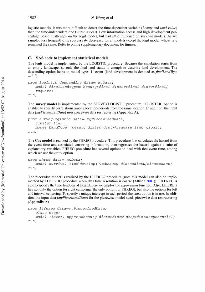
logistic models, it was more difficult to detect the time-dependent variable (beauty and land value)than the time-independent one (water access). Low information access and high development per-centage posed challenges on the logit model, but had little influence on survival models. As wesampled less frequently, the success rate decreased for all models except the logit model, whose rateremained the same. Refer to online supplementary document for figures.

C. SAS code to implement statistical modelsThe logit model is implemented by the LOGISTIC procedure. Because the simulation starts froman empty landscape, so only the final land status is enough to describe land development. Thedescending option helps to model type ‘1’ event (land development is denoted as finalLandType= ‘1’).

proc logistic descending data= myData;model finalLandType= beauty&final distsc&final distw&final/rsquare;

run;

The survey model is implemented by the SURVEYLOGISTIC procedure. ‘CLUSTER’ option isenabled to specify correlations among location-periods from the same location. In addition, the inputdata (myPiecewisedData) uses piecewise data restructuring (Appendix A).

proc surveylogistic data= myPiecewisedData;cluster fid;model LandType= beauty distsc distw/rsquare link=glogit;

run;

The Cox model is realized by the PHREG procedure. This procedure first calculates the hazard fromthe event time and associated censoring information, then regresses the hazard against a suite ofexplanatory variables. PHREG procedure has several options to deal with tied event time, amongwhich we use the exact option.

proc phreg data= myData;model survival_time∗develop(0)=beauty distscdistw/ties=exact;

run;

The piecewise model is realized by the LIFEREG procedure (note this model can also be imple-mented by LOGISTIC procedure when data time resolution is coarse (Allison 2001)). LIFEREG isable to specify the time function of hazard; here we employ the exponential function. Also, LIFEREGhas not only the option for right censoring (the only option for PHREG), but also the options for leftand interval censoring. To specify a unique intercept in each period, the class option is in use. In addi-tion, the input data (myPiecewisedData) for the piecewise model needs piecewise data restructuring(Appendix A).

proc lifereg data=myPiecewisedData;class step;model (lower, upper)=beauty distscdistw step/dist=exponential;

run;

Dow

nloa

ded

by [

Mem

oria

l Uni

vers

ity o

f N

ewfo

undl

and]

at 1

3:52

02

Aug

ust 2

014