Embed Size (px)
Citation preview
Correspondence to: Lee R. Lynd, Thayer School of Engineering, Dartmouth College, Hanover, NH 03755, USA.
E-mail: [email protected]
© 2009 Society of Chemical Industry and John Wiley & Sons, Ltd 247
Modeling and Analysis
Comparative analysis of effi ciency, environmental impact, and process economics for mature biomass refi ning scenariosMark Laser, Thayer School of Engineering, Dartmouth College, Hanover, NH
Eric Larson, Princeton Environmental Institute, Princeton University, NJ
Bruce Dale, Michigan State University, East Lansing, MI
Michael Wang, Argonne National Laboratory, Argonne, IL
Nathanael Greene, Natural Resources Defense Council, New York, NY
Lee R. Lynd, Thayer School of Engineering, Dartmouth College, Hanover, NH
Received October 27, 2008; revised version received January 19, 2009; accepted January 19, 2009
Published online in Wiley InterScience (www.interscience.wiley.com); DOI: 10.1002/bbb.136
Biofuels, Bioprod. Bioref. 3:247–270 (2009)
Abstract: Fourteen mature technology biomass refi ning scenarios – involving both biological and thermochemi-
cal processing with production of fuels, power, and/or animal feed protein – are compared with respect to process
effi ciency, environmental impact – including petroleum use, greenhouse gas (GHG) emissions, and water use–and
economic profi tability. The emissions analysis does not account for carbon sinks (e.g., soil carbon sequestration)
or sources (e.g., forest conversion) resulting from land-use considerations. Sensitivity of the scenarios to fuel and
electricity price, feedstock cost, and capital structure is also evaluated. The thermochemical scenario producing only
power achieves a process effi ciency of 49% (energy out as power as a percentage of feedstock energy in), 1359
kg CO2 equivalent avoided GHG emissions per Mg feedstock (current power mix basis) and a cost of $0.0575/kWh
($16/GJ), at a scale of 4535 dry Mg feedstock/day, 12% internal rate of return, 35% debt fraction, and 7% loan rate.
Thermochemical scenarios producing fuels and power realize effi ciencies between 55 and 64%, avoided GHG emis-
sions between 1000 and 1179 kg/dry Mg, and costs between $0.36 and $0.57 per liter gasoline equivalent
($1.37 – $2.16 per gallon) at the same scale and fi nancial structure. Scenarios involving biological production of
ethanol with thermochemical production of fuels and/or power result in effi ciencies ranging from 61 to 80%, avoided
GHG emissions from 965 to 1,258 kg/dry Mg, and costs from $0.25 to $0.33 per liter gasoline equivalent ($0.96 to
248 © 2009 Society of Chemical Industry and John Wiley & Sons, Ltd | Biofuels, Bioprod. Bioref. 3:247–270 (2009); DOI: 10.1002/bbb
M Laser et al. Modeling and Analysis: Comparative analysis of mature biomass refining scenarios
$1.24/gallon). Most of the biofuel scenarios offer comparable, if not lower, costs and much reduced GHG emis-
sions (>90%) compared to petroleum-derived fuels. Scenarios producing biofuels result in GHG displacements that
are comparable to those dedicated to power production (e.g., >825 kg CO2 equivalent/dry Mg biomass), especially
when a future power mix less dependent upon fossil fuel is assumed. Scenarios integrating biological and thermo-
chemical processing enable waste heat from the thermochemical process to power the biological process, resulting
in higher overall process effi ciencies than would otherwise be realized – effi ciencies on par with petroleum-based
fuels in several cases. © 2009 Society of Chemical Industry and John Wiley & Sons, Ltd
Keywords: biomass; biorefi nery; effi ciency; economics; environment; energy; biofuels
lower-than-assumed ethanol yield would be compensated
for by higher yields of F-T fuels and/or power, resulting
in relatively similar overall effi ciency and fossil fuel
displacement.
Technical and economic studies comparing processes
involving biological and/or thermochemical biomass
conversion exist in the literature. So and Brown,8 for
example, compared fast pyrolysis, simultaneous saccha-
rification and fermentation (SSF), and acid hydrolysis, all
producing ethanol. They concluded that the three proc-
esses have comparable capital, operating, and ethanol
production costs, and recommended further research on
the pyrolysis process to verify its feasibility. Wright and
Brown9 evaluated processes producing corn ethanol (dry
grind process), cellulosic ethanol (enzymatic hydrolysis),
methanol (gasification and synthesis), hydrogen (gasi-
fication), and F-T fuels ( gasification and synthesis),
assuming first-generation technology for the cellulosic
biomass processes. The authors concluded that biological
and thermochemical processing had comparable capital
costs ($3.60–$5.70 per annual gallon gasoline equivalent)
and operating costs ($1.05–$1.80 per gallon gasoline
equivalent), and that both platforms could compete with
corn ethanol when corn was priced at more than $3/
bushel. Piccolo and Bezzo10 compared ethanol produced
biologically via separate hydrolysis and fermentation
with that produced thermochemically through gasifi-
cation and synthesis, concluding that the gasification
process would require substantial technological improve-
ments before it could be cost competitive with biological
processing.
Th e RBAEF analysis, to our knowledge, is the fi rst to
compare the technologies in their mature context – i.e., a
state of advancement such that additional R&D eff ort would
Introduction
The Role of Biomass in America’s Energy Future
(RBAEF) project was initiated to identify and evaluate
paths by which biomass can make a large contribu-
tion to energy services. In the present study, we compare a
variety of biomass conversion technologies – including both
biological and thermochemical processing – and multiple
biorefi ning confi gurations producing fuels, power, and/or
animal feed protein. Th e work builds directly upon other
papers appearing in this issue1–7 and focuses on mature
technology, an emphasis that is supported by the realiza-
tion that answers to many important public policy questions
– including evaluating the long-term potential of energy
supply based on biomass-based technologies, the appropriate
level of support these technologies merit, and reconciling
land-use concerns – depends more on future achievable
performance than on today’s performance. Although there
is inherent uncertainty in projecting future technology,
there are also several factors that make such projections
more robust than they might at fi rst appear. Th e economics
of both existing mature energy production technologies
(e.g., oil refi ning) and projected mature biomass refi ning
(herein) are dominated by the cost of feedstock, not the
cost of processing. As a result, cost estimates for mature
process technology can be substantially diff erent from what
is actually achieved, while overall production costs and
conclusions about cost competiveness will not be aff ected
signifi cantly. Similarly, the process yields and effi ciencies
projected in this study – which determine quantities such
as greenhouse gas (GHG) emission reductions – do not, in
general, exhibit a large sensitivity to assumed performance
parameters. In a scenario producing ethanol,
Fischer-Tropsch F-T fuels and power, for example, a
© 2009 Society of Chemical Industry and John Wiley & Sons, Ltd | Biofuels, Bioprod. Bioref. 3:247–270 (2009); DOI: 10.1002/bbb 249
Modeling and Analysis: Comparative analysis of mature biomass refining scenarios M Laser et al.
off er only incremental improvement in cost reduction or
benefi t realization. As described in Lynd et al.,1 the issue’s
introductory paper, performance parameters were selected
consistent with the above operational defi nition according
to a knowledgeable optimist’s most likely estimate. Th is is
neither the optimist’s best-case estimate, nor the average,
most likely estimate of experts spanning the optimist–
pessimist spectrum. Estimates were made by members of
the project team with some consultation with experts not
part of the project, but without a systematic survey of such
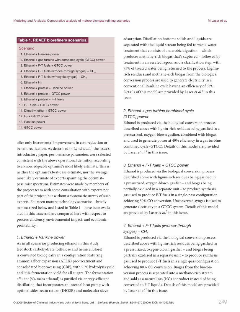
experts. Fourteen mature technology scenarios – briefl y
summarized below and listed in Table 1 – have been evalu-
ated in this issue and are compared here with respect to
process effi ciency, environmental impact, and economic
profi tability.
1. Ethanol + Rankine power
As in all scenarios producing ethanol in this study,
feedstock carbohydrate (cellulose and hemicellulose)
is converted biologically in a confi guration featuring
ammonia fi ber expansion (AFEX) pre-treatment and
consolidated bioprocessing (CBP), with 95% hydrolysis yield
and 95% fermentation yield for all sugars. Th e fermentation
effl uent (5% mass ethanol) is purifi ed via energy-effi cient
distillation that incorporates an internal heat pump with
optimal sidestream return (IHOSR) and molecular sieve
adsorption. Distillation bottoms solids and liquids are
separated with the liquid stream being fed to waste-water
treatment that consists of anaerobic digestion – which
produces methane-rich biogas that’s captured – followed by
treatment in an aerated lagoon and a clarifi cation step, with
95% of treated water being returned to the process. Lignin-
rich residues and methane-rich biogas from the biological
conversion process are used to generate electricity in a
conventional Rankine cycle having an effi ciency of 33%.
Details of this model are provided by Laser et al.5 in this
issue.
2. Ethanol + gas turbine combined cycle
(GTCC) power
Ethanol is produced via the biological conversion process
described above with lignin-rich residues being gasifi ed in a
pressurized, oxygen-blown gasifi er, combined with biogas,
and used to generate power at 49% effi ciency in a gas turbine
combined cycle (GTCC). Details of this model are provided
by Laser et al.5 in this issue.
3. Ethanol + F-T fuels + GTCC power
Ethanol is produced via the biological conversion process
described above with lignin-rich residues being gasifi ed in
a pressurized, oxygen-blown gasifi er – and biogas being
partially oxidized in a separate unit – to produce synthesis
gas used to produce F-T fuels in a single-pass confi guration
achieving 80% CO conversion. Unconverted syngas is used to
generate electricity in a GTCC system. Details of this model
are provided by Laser et al.7 in this issue.
4. Ethanol + F-T fuels (w/once-through
syngas) + CH4
Ethanol is produced via the biological conversion process
described above with lignin-rich residues being gasifi ed in
a pressurized, oxygen-blown gasifi er – and biogas being
partially oxidized in a separate unit – to produce synthesis
gas used to produce F-T fuels in a single-pass confi guration
achieving 80% CO conversion. Biogas from the biocon-
version process is separated into a methane-rich stream
and sold as a natural gas (NG) coproduct instead of being
converted to F-T liquids. Details of this model are provided
by Laser et al.7 in this issue.
Table 1. RBAEF biorefinery scenarios.
Scenario 1. Ethanol + Rankine power
2. Ethanol + gas turbine with combined cycle (GTCC) power
3. Ethanol + F-T fuels + GTCC power
4. Ethanol + F-T fuels (w/once-through syngas) + CH4
5. Ethanol + F-T fuels (w/recycle syngas) + CH4
6. Ethanol + H2
7. Ethanol + protein + Rankine power
8. Ethanol + protein + GTCC power
9. Ethanol + protein + F-T fuels
10. F-T fuels + GTCC power
11. Dimethyl ether + GTCC power
12. H2 + GTCC power
13. Rankine power
14. GTCC power
250 © 2009 Society of Chemical Industry and John Wiley & Sons, Ltd | Biofuels, Bioprod. Bioref. 3:247–270 (2009); DOI: 10.1002/bbb
M Laser et al. Modeling and Analysis: Comparative analysis of mature biomass refining scenarios
5. Ethanol + F-T fuels (w/recycle syngas) + CH4
Ethanol is produced via the biological conversion process
described above with lignin-rich residues being gasifi ed in
a pressurized, oxygen-blown gasifi er – and biogas being
partially oxidized in a separate unit – to produce synthesis
gas used to produce F-T fuels. Unconverted syngas is recy-
cled back to the F-T synthesis block with unconverted light-
end gases being combined with biogas methane to form a
NG coproduct. Details of this model are provided by Laser et
al. 7 in this issue.
6. Ethanol + H2
Ethanol is produced via the biological conversion process
described above with lignin-rich residues being gasifi ed
in a pressurized oxygen-blown gasifi er – and biogas being
partially oxidized in a separate unit – to produce synthesis
gas from which hydrogen is separated via pressure swing
adsorption (PSA). Details of this model are provided by
Laser et al.7 in this issue.
7. Ethanol + protein + Rankine power
Ethanol is produced via biological conversion similar to
the process described above, but including aqueous protein
extraction that occurs in two stages – one before AFEX
pre-treatment, and one aft er achieving 84% total extrac-
tion. Lignin-rich residues and methane-rich biogas from the
biological conversion process are used to generate electricity
in a conventional Rankine cycle. Details of this model are
provided by Laser et al.7 in this issue.
8. Ethanol + protein + GTCC power
Ethanol and protein are coproduced via biological
conversion as described above. Lignin-rich residues are
gasifi ed in a pressurized, oxygen-blown gasifi er, combined
with biogas, and used to generate power in a GTCC system.
Details of this model are provided by Laser et al.7 in this
issue.
9. Ethanol + protein + F-T fuels
Ethanol and protein are coproduced via biological conver-
sion as described above. Lignin-rich residues are gasifi ed
in a pressurized, oxygen-blown gasifi er – and biogas is
partially oxidized in a separate unit – to produce synthesis
gas used to produce F-T fuels in a single-pass confi guration.
Unconverted syngas is used to generate electricity in a
GTCC system. Details of this model are provided by Laser et
al.7 in this issue.
10. F-T fuels + GTCC power
Switchgrass feedstock is gasifi ed in a pressurized, oxygen-
blown gasifi er, producing synthesis gas used to produce F-T
fuels in a single-pass confi guration. Unconverted syngas is
converted to electricity in a GTCC system. Details of this
model are provided by Larson et al.4 in this issue.
11. DME + GTCC power
Switchgrass feedstock is gasifi ed in a pressurized, oxygen-
blown gasifi er, producing synthesis gas used to produce
dimethyl ether (DME) in a single-pass confi guration.
Unconverted syngas is converted to electricity in a GTCC
system. Details of this model are provided by Larson et al.4
in this issue.
12. H2 + GTCC power
Switchgrass feedstock is gasifi ed in a pressurized, oxygen-
blown gasifi er, producing synthesis gas from which
hydrogen is separated via pressure swing adsorption.
Unconverted syngas is converted to electricity in a GTCC
system. Details of this model are provided by Larson et al.4
in this issue.
13. Rankine power
Switchgrass feedstock is used to generate electricity in
a conventional Rankine cycle having an effi ciency of
33%. Details of this model are provided by Jin et al.3 in this
issue.
14. GTCC power
Switchgrass feedstock is gasifi ed in a pressurized oxygen-
blown gasifi er and used to generate power at 49% effi ciency
in a GTCC system. Details of this model are provided by Jin
et al.3 in this issue.
Each scenario assumes a scale of 4535 dry Mg feedstock/
day, the use of switchgrass having a delivered cost of $49/
Mg, a capital structure of 35% debt fi nancing, electricity
price of $0.05/kWh, internal rate of return of 12% and a
© 2009 Society of Chemical Industry and John Wiley & Sons, Ltd | Biofuels, Bioprod. Bioref. 3:247–270 (2009); DOI: 10.1002/bbb 251
Modeling and Analysis: Comparative analysis of mature biomass refining scenarios M Laser et al.
2006 cost year.* As part of the comparison, sensitivity of
the scenarios to several variables – including fuel and elec-
tricity price, feedstock cost, and capital structure – was also
evaluated.
As noted in Lynd et al., 1 this issue’s introductory paper,
diff erent technologies diff er substantially with respect to
their current state of development, and may also diff er
in the extent to which features of mature technology can
be anticipated. While comparisons are presented in this
paper on a side-by-side basis, we recognize uncertainties
inherent in comparing performance and cost projection
for diff erent mature technologies. For thermochemical
processing, cost and performance for most of the unit
operations (e.g., gasifi cation, power generation via GTCC,
fuel synthesis) are largely based on existing commercial or
demonstration plants, though some key projected improve-
ments, such as integrated tar cracking and gas clean-up,
have yet to be realized at scale. Fermentative production
of ethanol is the basis for production of over 38 billion
liters (10 billion gallons) annually, but a key aspect of the
mature biological processing scenarios, CBP, is still under
development. Detailed understanding and well-developed
predictive capability support the feasibility of organism
development for CBP.5 A substantial eff ort to standardize
costs and accounting assumptions was made in an eff ort to
make results for the various technologies as comparable as
possible, as described in Lynd et al.1 In particular, the same
designs, performance assumptions and costs were assumed
for stand-alone power generation, power generation from
residues in cellulosic ethanol production, and power cogen-
eration in conjunction with production of thermochemical
fuels. For all scenarios examined in this study, the largest
capital cost – ranging from 70% to 100% – is for operations
necessary for power and steam generation, including feed
preparation, gasifi cation, syngas cooling and clean-up, air
separation, and the power island. Cost estimates for unit
operations directly involved in biological fuel production
and production of thermochemical fuels were developed
separately. Th is introduces an element of uncertainty in
* The purchased equipment cost year is indexed to the analysis cost year, 2006,
using the Chemical Engineering Plant Cost Index. Costs for chemicals are
indexed to the analysis cost year using the Industrial Chemicals Producer Price
Index published by the US Department of Labor Bureau of Labor Statistics.
making cross-technology cost comparisons. Separately
developed cost estimates are, however, diffi cult to avoid
and may well refl ect reality in light of the rather diff erent
equipment involved: largely high-pressure and gas-phase
for thermochemical fuel synthesis, largely low-pressure and
aqueous-phase for biological fermentation.
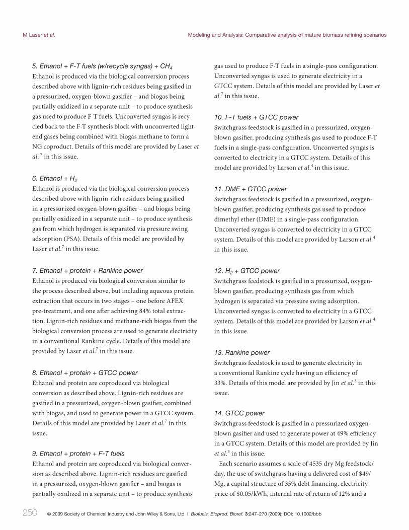
Process effi ciency
Th e mature technology designs make extensive use of ‘waste’
heat that would otherwise be lost to the environment.
Although waste-heat utilization involves added capital
cost and can be diffi cult to accomplish at large scales, the
payoff is signifi cantly higher process effi ciencies, resulting
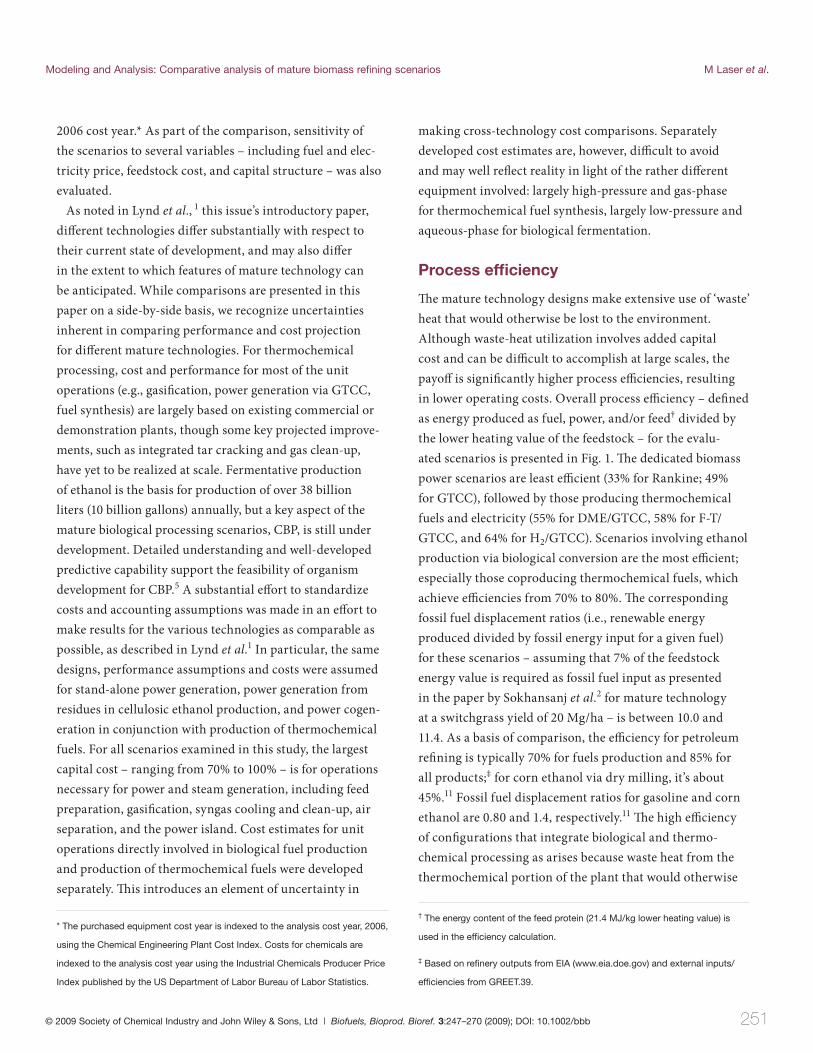
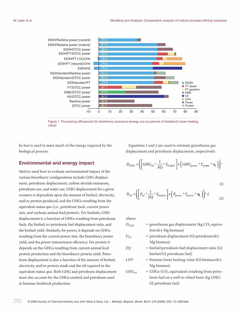
in lower operating costs. Overall process effi ciency – defi ned
as energy produced as fuel, power, and/or feed† divided by
the lower heating value of the feedstock – for the evalu-
ated scenarios is presented in Fig. 1. Th e dedicated biomass
power scenarios are least effi cient (33% for Rankine; 49%
for GTCC), followed by those producing thermochemical
fuels and electricity (55% for DME/GTCC, 58% for F-T/
GTCC, and 64% for H2/GTCC). Scenarios involving ethanol
production via biological conversion are the most effi cient;
especially those coproducing thermochemical fuels, which
achieve effi ciencies from 70% to 80%. Th e corresponding
fossil fuel displacement ratios (i.e., renewable energy
produced divided by fossil energy input for a given fuel)
for these scenarios – assuming that 7% of the feedstock
energy value is required as fossil fuel input as presented
in the paper by Sokhansanj et al.2 for mature technology
at a switchgrass yield of 20 Mg/ha – is between 10.0 and
11.4. As a basis of comparison, the effi ciency for petroleum
refi ning is typically 70% for fuels production and 85% for
all products;‡ for corn ethanol via dry milling, it’s about
45%.11 Fossil fuel displacement ratios for gasoline and corn
ethanol are 0.80 and 1.4, respectively.11 Th e high effi ciency
of confi gurations that integrate biological and thermo-
chemical processing as arises because waste heat from the
thermochemical portion of the plant that would otherwise
† The energy content of the feed protein (21.4 MJ/kg lower heating value) is
used in the efficiency calculation.
‡ Based on refinery outputs from EIA (www.eia.doe.gov) and external inputs/
efficiencies from GREET.39.
252 © 2009 Society of Chemical Industry and John Wiley & Sons, Ltd | Biofuels, Bioprod. Bioref. 3:247–270 (2009); DOI: 10.1002/bbb
M Laser et al. Modeling and Analysis: Comparative analysis of mature biomass refining scenarios
be lost is used to meet much of the energy required by the
biological process.
Environmental and energy impact
Metrics used here to evaluate environmental impact of the
various biorefi nery confi gurations include GHG displace-
ment, petroleum displacement, carbon dioxide emissions,
petroleum use, and water use. GHG displacement for a given
scenario is dependent upon the amount of biofuel, electricity,
and/or protein produced, and the GHGs resulting from the
equivalent status quo (i.e., petroleum fuels, current power
mix, and soybean animal feed protein). For biofuels, GHG
displacement is a function of GHGs resulting from petroleum
fuels, the biofuel-to-petroleum fuel displacement ratio, and
the biofuel yield. Similarly, for power, it depends on GHGs
resulting from the current power mix, the biorefi nery power
yield, and the power transmission effi ciency. For protein it
depends on the GHGs resulting from current animal feed
protein production and the biorefi nery protein yield. Petro-
leum displacement is also a function of the amount of biofuel,
electricity, and/or protein made and the oil required in the
equivalent status quo. Both GHG and petroleum displacement
must also account for the GHGs emitted and petroleum used
in biomass feedstock production.
Equations 1 and 2 are used to estimate greenhouse gas
displacement and petroleum displacement, respectively:
D GHGEQ
Y GHG YGHG oil biofuel power po= ⎡⎣⎢
⎤⎦⎥
+* * *1
wwer t* *�⎡⎣ ⎤⎦⎛⎝⎜
⎞⎠⎟
(1)
D PEQ
Y P Yoil oil biofuel power power= ⎡⎣⎢
⎤⎦⎥
+* * * *1
��t L⎡⎣ ⎤⎦⎛⎝⎜
⎞⎠⎟
* (2)
where:
DGHG � greenhouse gas displacement (kg CO2 equiva-
lent/dry Mg biomass)
Doil � petroleum displacement (GJ petroleum/dry
Mg biomass)
EQ � biofuel:petroleum fuel displacement ratio (GJ
biofuel/GJ petroleum fuel)
LHV � biomass lower heating value (GJ biomass/dry
Mg biomass)
GHGoil � GHGs (CO2 equivalent) resulting from petro-
leum fuel on a well-to-wheel basis (kg GHG/
GJ petroleum fuel)
EtOH/Rankine power (mature)
EtOH/Rankine power (current)
EtOH/GTCC power 68.1EtOH/FT/GTCC power 70.4
EtOH/FT (1X)/CH4 76.5
EtOH/FT (recycle)/CH4 79.6
EtOH/H2 76.5
EtOH/protein/Rankine power 61.2
EtOH/protein/GTCC power 69.4
EtOH/protein/FT 73.3
FT/GTCC power 57.7
DME/GTCC power 54.9
H2/GTCC power 64.2
-10 0 10 20 30 40 50 60 70 80 90
Rankine power 32.8
GTCC power 49.1
EtOHFT dieselFT gasolineDMEH2CH4PowerProtein
61.4
43.3
Figure 1. Processing effi ciencies for biorefi nery scenarios (energy out as percent of feedstock lower heating value).
© 2009 Society of Chemical Industry and John Wiley & Sons, Ltd | Biofuels, Bioprod. Bioref. 3:247–270 (2009); DOI: 10.1002/bbb 253
Modeling and Analysis: Comparative analysis of mature biomass refining scenarios M Laser et al.
GHGpower � GHGs (CO2 equivalent) resulting from power
on a fuel extraction-to-end use basis (kg
GHG/GJ power)
GHGprotein � GHGs (CO2 equivalent) resulting from
animal feed protein on full life cycle basis (kg
GHG/kg protein)
GHGbiomass � GHGs (CO2 equivalent) resulting from
biomass production, including farming,
harvesting, and transportation to biorefi nery
(kg GHG/dry Mg biomass)
Poil � petroleum used to produce petroleum fuel
(GJ petroleum/GJ petroleum fuel)
Ppower � petroleum used to produce power (GJ petro-
leum/GJ power)
Pprotein � petroleum used to produce animal feed
protein (GJ petroleum/kg protein)
Pbiomass � petroleum used to produce biomass (GJ
petroleum/dry Mg biomass)
Ybiofuel � biofuel yield (GJ biofuel/GJ biomass)
Ypower � power yield (GJ power/GJ biomass)
Yprotein � protein yield (kg protein/dry Mg biomass)
ηt � power transmission effi ciency
Th e fi rst term in each equation calculates displacement
resulting from biofuels production in the biorefi nery; the
second, displacement from power production; and the third
from protein coproduction (if applicable). Th e fi nal term
accounts for GHG emissions and petroleum used during
production of the biomass feedstock, and therefore has a
negative sign.
Field-to-wheels carbon dioxide emissions account for
emissions from biomass production; biofuels production;
biofuel transportation, storage, and distribution; and vehicle
operation and are calculated using the following equations:
E E E E E UFTW biomass process TSD vehicle bioma= + + + − sss (3)
E CY VE
biomass biomassfuel
=⎛
⎝⎜
⎞
⎠⎟
⎛⎝⎜
⎞⎠⎟
1 1 (4)
E C CF
LHprocess process credit= −( )⎛⎝⎜
⎞⎠⎟
⎡⎣⎢
⎤⎦⎥
1VV
VEgasoline( )⎛
⎝⎜⎞⎠⎟
1 (5)
E CY VE
TSD TSDfuel
=⎛
⎝⎜
⎞
⎠⎟
⎛⎝⎜
⎞⎠⎟
1 1 (6)
E C LHVVE
vehicle combust gasoline= ( )( )⎛⎝⎜
⎞⎠⎟
1 (7)
U E Ebiomass process vehicle= + (8)
where:
EFTW � fi eld-to-wheel emissions for biofuel produc-
tion (g CO2/km)
Ebiomass � emissions from biomass production (g CO2/
km)
Eprocess � emissions from biofuel production process (g
CO2/km)
ETSD � emissions from biofuel transportation,
storage, and distribution (g CO2/km)
Evehicle � emissions from vehicle operation using
biofuels (g CO2/km)
Ubiomass � carbon uptake resulting from biomass
growth (g CO2/km)
Cbiomass � emissions resulting from biomass production
(g CO2/dry Mg biomass)
Yfuel � biofuel yield (liters gasoline equivalent/dry
Mg biomass)
VE � vehicle effi ciency (km/L)
Cprocess � emissions from biofuel process (g CO2/hr)
Ccredit � coproduct emissions credit (g CO2/hr)
F � biofuel production rate (GJ/hr)
LHVgasoline � lower heating value of gasoline (GJ/L)
CTSD � emissions from transportation, storage, and
distribution of biofuel (g CO2/GJ fuel)
Ccombust � emissions from biofuel combustion in vehicle
(g CO2/GJ fuel)
Here, it is assumed that CO2 released during fuel production
and vehicle operation – which involves only biomass and no
fossil fuel in these scenarios – exactly matches that assimi-
lated by the feedstock biomass during growth (i.e., Eqn 8).
Field-to-wheel emissions are therefore primarily dependent
upon feedstock production; fuel yield; fuel transportation,
storage, and distribution; and vehicle effi ciency. We have not
accounted for carbon sinks (e.g., soil carbon sequestration)
254 © 2009 Society of Chemical Industry and John Wiley & Sons, Ltd | Biofuels, Bioprod. Bioref. 3:247–270 (2009); DOI: 10.1002/bbb
M Laser et al. Modeling and Analysis: Comparative analysis of mature biomass refining scenarios
or sources (e.g., forest conversion) resulting from land use
changes such as those analyzed by Searchinger et al.12 and
Fargione et al.13 We do recognize the importance of such
considerations, though they are beyond the scope of this
study for which the focus is biomass processing. Wu et
al.14 conducted a more detailed fuel lifecycle assessment
for a subset of the scenarios presented in this study (Table
1, Scenarios 1, 2, 3, 7, 10, and 11). Th eir analysis, which
assumes that 39% of the switchgrass feedstock is grown on
cropland, does account for soil carbon sequestration benefi ts
resulting from converting this land from conventional row
crops to switchgrass.
Petroleum use for the mature biorefi ning scenarios –
which is limited to biomass production and fuel transporta-
tion, storage, and distribution, as no petroleum is used in
the biorefi nery – is calculated using Eqn 9:
OIL O OY VE
biomass TSDfuel
= +( )⎛
⎝⎜
⎞
⎠⎟
⎛⎝⎜
⎞⎠⎟
1 1 (9)
where:
OIL � petroleum requirement for biofuel production
(GJ/km)
Obiomass � petroleum required for biomass production (GJ/
dry Mg biomass)
OTSD � petroleum required for biofuel transportation,
storage, and distribution (GJ/dry Mg biomass)
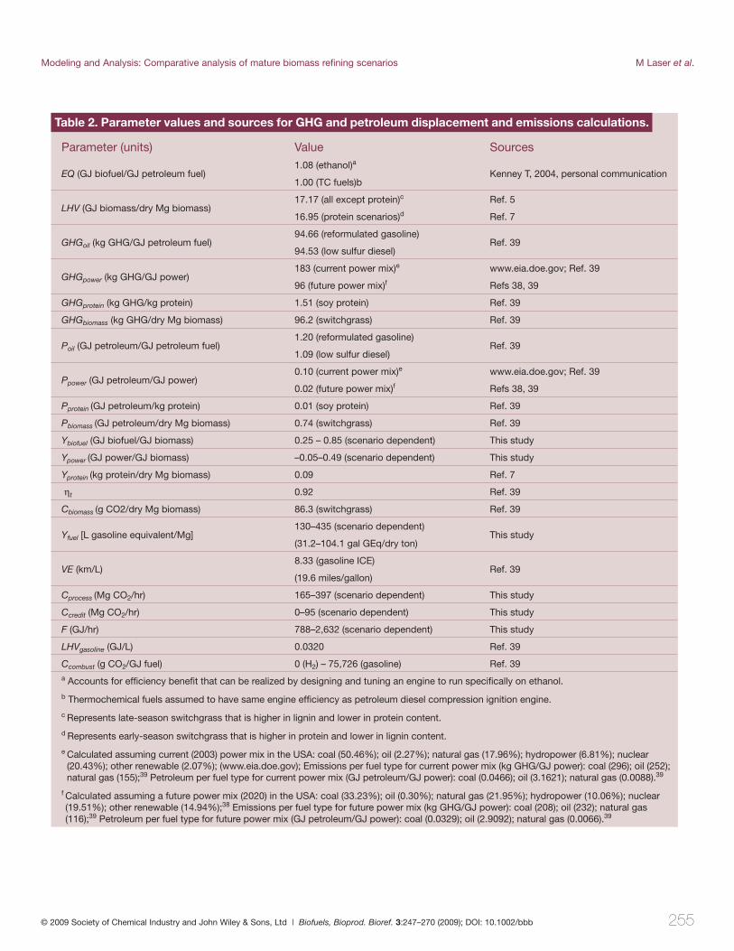
Values for and sources of the parameters used in the above
calculations are listed in Table 2. Figures 2 and 3 present
results for GHG and petroleum displacement, respectively.
Scenarios producing biofuels result in GHG displacements
that are comparable to those dedicated to power production
(e.g., � 825 kg CO2 equivalent/dry Mg biomass), especially
when a future power mix less dependent upon fossil fuel is
assumed. Th is runs counter to the conventional notion that
potential GHG emissions reductions are higher for biomass
power production than for biofuels production,15,16 since it
is typically assumed that biopower would replace coal power.
While GHG emissions per unit delivered energy are indeed
much greater for electricity than for fuels with the current
power mix (coal 50.5%, nuclear 20.4%, natural gas 18.0%,
hydro 6.8%, oil 2.3%, other renewables 2.1% (www.eia.doe.
gov)) – 183 vs. 95 kg CO2 equivalent/GJ (Table 2) – the
potentially high biofuel yields calculated in many of the
mature technology scenarios compared to the mature
power-only scenarios lead to comparable GHG emissions
displacement potential when a future power mix is assumed.
As the electricity system becomes decarbonized to a greater
extent in the future,17 the GHG benefi t of biomass used for
fuel production will increase relative to the benefi t of using
biomass for power generation.
When considering petroleum displacement, it’s important
to note that only about 2% of the current US power mix
is derived directly from oil (www.eia.doe.gov), and little
petroleum is used in the production of power from other
sources (Table 2). In fact, petroleum displacement for
dedicated electricity production from biomass is zero or
negative – i.e., more petroleum is required to produce the
biomass than is displaced by the power produced from the
biomass – for the scenarios evaluated here. Fuels produced
using biological conversion also displace more petroleum
than do fuels produced solely from thermochemical
processing, as biological conversion scenarios have higher
fuel yields (recall Fig. 1).
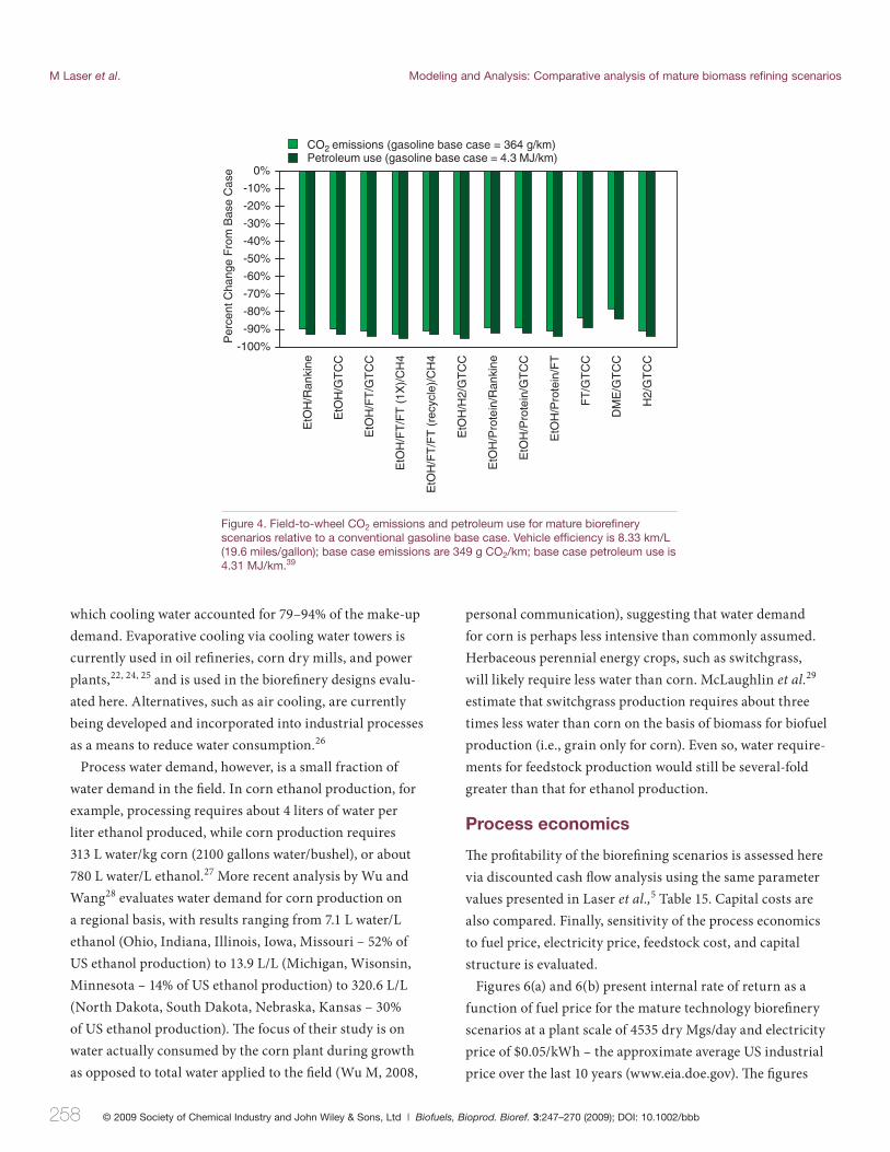
Figure 4 presents results for CO2 emissions and petroleum
use as a percent change relative to a conventional gasoline
base case. Scenarios involving biological ethanol all result in
CO2 emissions that are about 90% lower than the gasoline
base case and petroleum use that is more than 92% lower.
If soil carbon sequestration is accounted for – using the
same value as assumed by Wu et al.14 (53,471 g CO2/dry Mg
biomass) – then CO2 emissions for the bioethanol scenarios
become at least 96% lower than the base case. Th e thermo-
chemical fuels scenarios result in 78%, 84%, and 91% CO2
reduction and 84%, 89%, and 94% petroleum use reduction
for DME, F-T fuels, and H2, respectively. When soil carbon
sequestration is accounted for, CO2 emissions become 91%,
94%, and 96% lower than the base case for DME, F-T fuels,
and H2, respectively. Th ese results correspond reasonably
well to Wu et al.,14 who found that GHG emissions are
reduced by 82% to 87% (E85 basis) and petroleum use by
more than 90% relative to the base case.
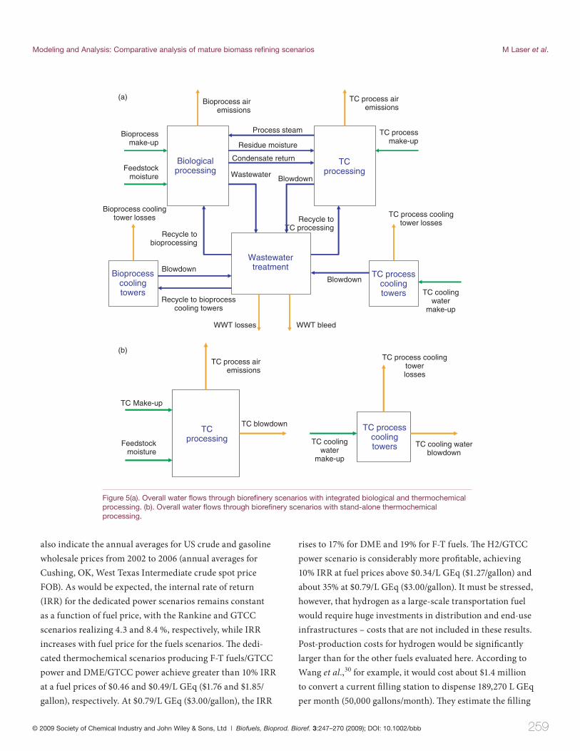
Figures 5(a) and 5(b) illustrate the overall water fl ows
through the integrated bioprocessing/thermochemical and
standalone thermochemical confi gurations, respectively.
Water balance and make-up requirement results for each
© 2009 Society of Chemical Industry and John Wiley & Sons, Ltd | Biofuels, Bioprod. Bioref. 3:247–270 (2009); DOI: 10.1002/bbb 255
Modeling and Analysis: Comparative analysis of mature biomass refining scenarios M Laser et al.
Table 2. Parameter values and sources for GHG and petroleum displacement and emissions calculations.
Parameter (units) Value Sources
EQ (GJ biofuel/GJ petroleum fuel)1.08 (ethanol)a
Kenney T, 2004, personal communication1.00 (TC fuels)b
LHV (GJ biomass/dry Mg biomass)17.17 (all except protein)c Ref. 5
16.95 (protein scenarios)d Ref. 7
GHGoil (kg GHG/GJ petroleum fuel)94.66 (reformulated gasoline)
Ref. 3994.53 (low sulfur diesel)
GHGpower (kg GHG/GJ power)183 (current power mix)e www.eia.doe.gov; Ref. 39
96 (future power mix)f Refs 38, 39
GHGprotein (kg GHG/kg protein) 1.51 (soy protein) Ref. 39
GHGbiomass (kg GHG/dry Mg biomass) 96.2 (switchgrass) Ref. 39
Poil (GJ petroleum/GJ petroleum fuel)1.20 (reformulated gasoline)
Ref. 391.09 (low sulfur diesel)
Ppower (GJ petroleum/GJ power)0.10 (current power mix)e www.eia.doe.gov; Ref. 39
0.02 (future power mix)f Refs 38, 39
Pprotein (GJ petroleum/kg protein) 0.01 (soy protein) Ref. 39
Pbiomass (GJ petroleum/dry Mg biomass) 0.74 (switchgrass) Ref. 39
Ybiofuel (GJ biofuel/GJ biomass) 0.25 – 0.85 (scenario dependent) This study
Ypower (GJ power/GJ biomass) –0.05–0.49 (scenario dependent) This study
Yprotein (kg protein/dry Mg biomass) 0.09 Ref. 7
ηt 0.92 Ref. 39
Cbiomass (g CO2/dry Mg biomass) 86.3 (switchgrass) Ref. 39
Yfuel [L gasoline equivalent/Mg]130–435 (scenario dependent)
This study(31.2–104.1 gal GEq/dry ton)
VE (km/L)8.33 (gasoline ICE)
Ref. 39(19.6 miles/gallon)
Cprocess (Mg CO2/hr) 165–397 (scenario dependent) This study
Ccredit (Mg CO2/hr) 0–95 (scenario dependent) This study
F (GJ/hr) 788–2,632 (scenario dependent) This study
LHVgasoline (GJ/L) 0.0320 Ref. 39
Ccombust (g CO2/GJ fuel) 0 (H2) – 75,726 (gasoline) Ref. 39a Accounts for effi ciency benefi t that can be realized by designing and tuning an engine to run specifi cally on ethanol.
b Thermochemical fuels assumed to have same engine effi ciency as petroleum diesel compression ignition engine.
c Represents late-season switchgrass that is higher in lignin and lower in protein content.
d Represents early-season switchgrass that is higher in protein and lower in lignin content.
e Calculated assuming current (2003) power mix in the USA: coal (50.46%); oil (2.27%); natural gas (17.96%); hydropower (6.81%); nuclear (20.43%); other renewable (2.07%); (www.eia.doe.gov); Emissions per fuel type for current power mix (kg GHG/GJ power): coal (296); oil (252); natural gas (155);39 Petroleum per fuel type for current power mix (GJ petroleum/GJ power): coal (0.0466); oil (3.1621); natural gas (0.0088).39
f Calculated assuming a future power mix (2020) in the USA: coal (33.23%); oil (0.30%); natural gas (21.95%); hydropower (10.06%); nuclear (19.51%); other renewable (14.94%);38 Emissions per fuel type for future power mix (kg GHG/GJ power): coal (208); oil (232); natural gas (116);39 Petroleum per fuel type for future power mix (GJ petroleum/GJ power): coal (0.0329); oil (2.9092); natural gas (0.0066).39

256 © 2009 Society of Chemical Industry and John Wiley & Sons, Ltd | Biofuels, Bioprod. Bioref. 3:247–270 (2009); DOI: 10.1002/bbb
M Laser et al. Modeling and Analysis: Comparative analysis of mature biomass refining scenarios
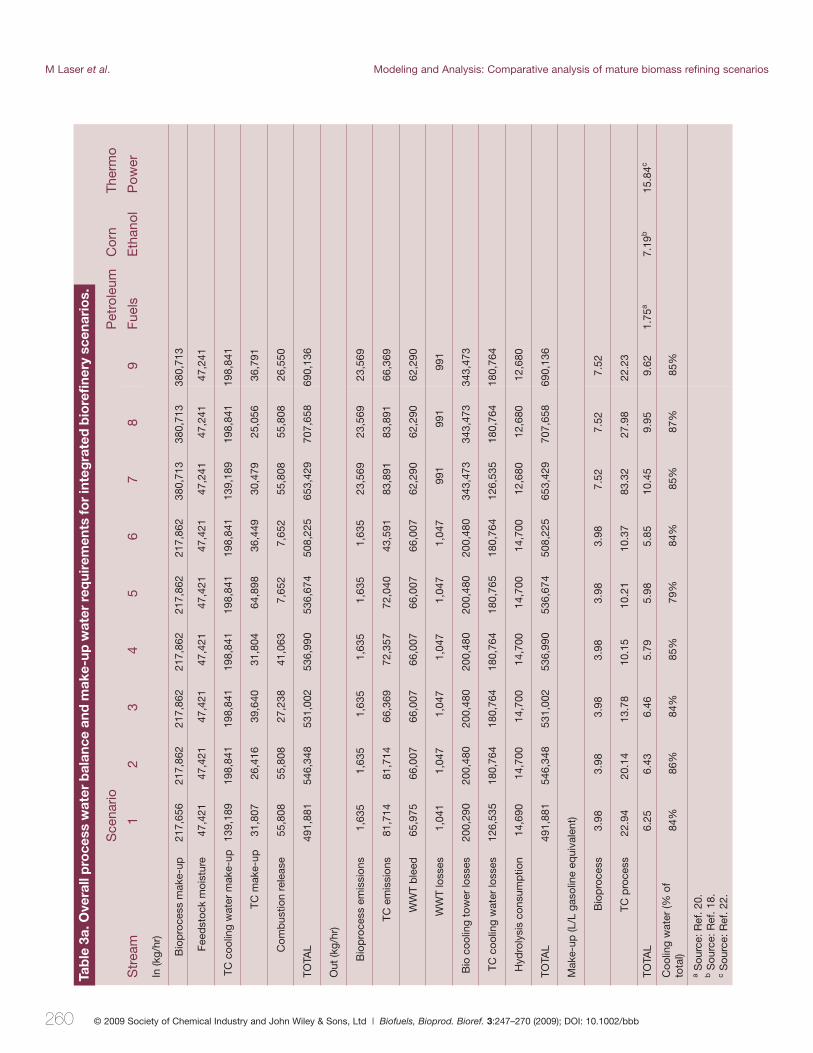
scenario are listed in Tables 3(a) and 3(b). In the integrated
scenarios without protein coproduction, the total make-up
water requirement – to account for cooling tower evapora-
tion and windage losses, water in vapor streams vented to
atmosphere, and water consumed in hydrolysis reactions
– ranges from 5.8 to 6.5 liter per liter gasoline equivalent,
denoted L GEq throughout the rest of the paper. Make-up
water for only the biological processing portion of the plant
producing ethanol is about 4.0 L/L GEq. As a point of refer-
ence, this value compares favorably to corn ethanol produc-
tion which requires, on average, about 6.1 L/L GEq (4 L/L
ethanol),18 or about 6.6 L/L GEq when water needed for
process power is included (0.17 kWh/L ethanol19).§ Estimates
of water use for petroleum fuels vary signifi cantly, from as
low as 1–2.5 L water/L GEq20 to several-fold higher –
10–40 L/L GEq, for example.21 Conventional thermoelectric
power requires about 15.8 L/L GEq (1.8 L/kWh). 22 We note
that comparisons between confi gurations in this study are
on common basis; the same cannot necessarily be said of
comparisons between this study and others.
§ Estimate is as follows: 0.17 kW/L ethanol*1.89 L water/kW � 0.33 L water/L
ethanol � 0.5 L water/L gasoline equivalent. Corn ethanol power requirement
from Wallace et al.19; water for thermoelectric power production from Torcellini22.
0
200
400
600
800
1.000
1.200
1.400
1.600
EtO
H/R
anki
ne
EtO
H/G
TC
C
EtO
H/F
T/G
TC
C
EtO
H/F
T (
1X)/
CH
4
EtO
H/F
T (
recy
cle)
/CH
4
EtO
H/H
2
EtO
H/P
rote
in/R
anki
ne
EtO
H/P
rote
in/G
TC
C
EtO
H/P
rote
in/F
T
FT
/GT
CC
DM
E/G
TC
C H2
Ran
kine
GT
CC
GH
G D
ispl
acem
ent (
kg C
O2
equi
vale
nt/M
g)
Hypothetical displacement for 100% biofuel yield
Renewables
Nuclear
Hydropower
Natural Gas
Oil
Coal
Power Mix (%)
14.942.07
19.5120.43
10.066.81
21.9517.96
0.302.27
33.2350.46
A FutureCurrent
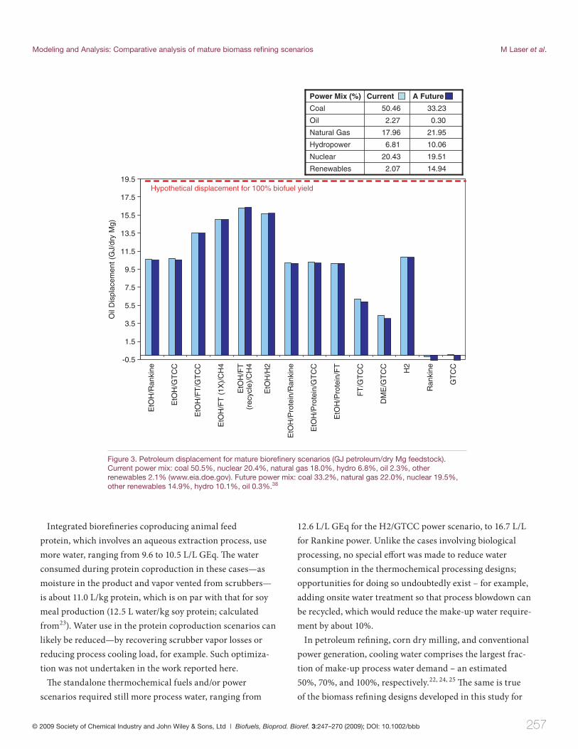
Figure 2. Greenhouse gas displacement for mature biorefi nery scenarios (kg GHG/dry Mg feedstock). Current power mix: coal 50.5%, nuclear 20.4%, natural gas 18.0%, hydro 6.8%, oil 2.3%, other renewables 2.1% (www.eia.doe.gov). Future power mix: coal 33.2%, natural gas 22.0%, nuclear 19.5%, other renewables 14.9%, hydro 10.1%, oil 0.3%.39
© 2009 Society of Chemical Industry and John Wiley & Sons, Ltd | Biofuels, Bioprod. Bioref. 3:247–270 (2009); DOI: 10.1002/bbb 257
Modeling and Analysis: Comparative analysis of mature biomass refining scenarios M Laser et al.
Integrated biorefi neries coproducing animal feed
protein, which involves an aqueous extraction process, use
more water, ranging from 9.6 to 10.5 L/L GEq. Th e water
consumed during protein coproduction in these cases—as
moisture in the product and vapor vented from scrubbers—
is about 11.0 L/kg protein, which is on par with that for soy
meal production (12.5 L water/kg soy protein; calculated
from23). Water use in the protein coproduction scenarios can
likely be reduced—by recovering scrubber vapor losses or
reducing process cooling load, for example. Such optimiza-
tion was not undertaken in the work reported here.
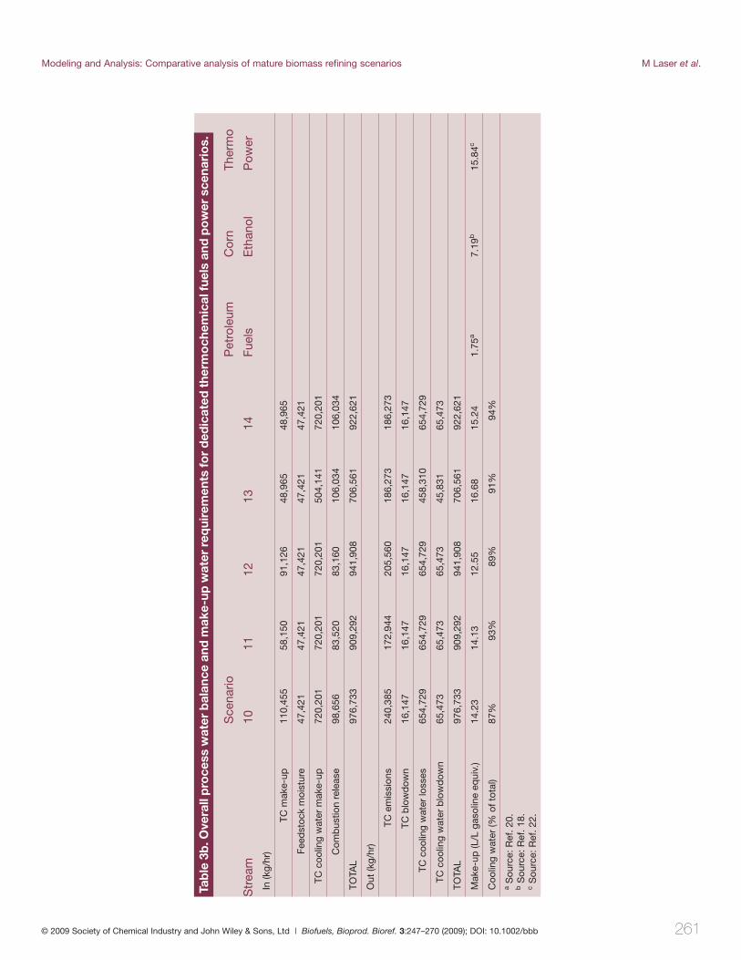
Th e standalone thermochemical fuels and/or power
scenarios required still more process water, ranging from
12.6 L/L GEq for the H2/GTCC power scenario, to 16.7 L/L
for Rankine power. Unlike the cases involving biological
processing, no special eff ort was made to reduce water
consumption in the thermochemical processing designs;
opportunities for doing so undoubtedly exist – for example,
adding onsite water treatment so that process blowdown can
be recycled, which would reduce the make-up water require-
ment by about 10%.
In petroleum refi ning, corn dry milling, and conventional
power generation, cooling water comprises the largest frac-
tion of make-up process water demand – an estimated
50%, 70%, and 100%, respectively.22, 24, 25 Th e same is true
of the biomass refi ning designs developed in this study for
-0.5
1.5
3.5
5.5
7.5
9.5
11.5
13.5
15.5
17.5
19.5
EtO
H/R
anki
ne
EtO
H/G
TC
C
EtO
H/F
T/G
TC
C
EtO
H/F
T (
1X)/
CH
4
EtO
H/F
T
(rec
ycle
)/C
H4
EtO
H/H
2
EtO
H/P
rote
in/R
anki
ne
EtO
H/P
rote
in/G
TC
C
EtO
H/P
rote
in/F
T
FT
/GT
CC
DM
E/G
TC
C H2
Ran
kine
GT
CC
Oil
Dis
plac
emen
t (G
J/dr
y M
g)
Hypothetical displacement for 100% biofuel yield
Renewables
Nuclear
Hydropower
Natural Gas
Oil
Coal
Power Mix (%)
14.942.07
19.5120.43
10.066.81
21.9517.96
0.302.27
33.2350.46
Current A Future
Figure 3. Petroleum displacement for mature biorefi nery scenarios (GJ petroleum/dry Mg feedstock). Current power mix: coal 50.5%, nuclear 20.4%, natural gas 18.0%, hydro 6.8%, oil 2.3%, other renewables 2.1% (www.eia.doe.gov). Future power mix: coal 33.2%, natural gas 22.0%, nuclear 19.5%, other renewables 14.9%, hydro 10.1%, oil 0.3%.38
258 © 2009 Society of Chemical Industry and John Wiley & Sons, Ltd | Biofuels, Bioprod. Bioref. 3:247–270 (2009); DOI: 10.1002/bbb
M Laser et al. Modeling and Analysis: Comparative analysis of mature biomass refining scenarios
which cooling water accounted for 79–94% of the make-up
demand. Evaporative cooling via cooling water towers is
currently used in oil refi neries, corn dry mills, and power
plants,22, 24, 25 and is used in the biorefi nery designs evalu-
ated here. Alternatives, such as air cooling, are currently
being developed and incorporated into industrial processes
as a means to reduce water consumption.26
Process water demand, however, is a small fraction of
water demand in the fi eld. In corn ethanol production, for
example, processing requires about 4 liters of water per
liter ethanol produced, while corn production requires
313 L water/kg corn (2100 gallons water/bushel), or about
780 L water/L ethanol.27 More recent analysis by Wu and
Wang28 evaluates water demand for corn production on
a regional basis, with results ranging from 7.1 L water/L
ethanol (Ohio, Indiana, Illinois, Iowa, Missouri – 52% of
US ethanol production) to 13.9 L/L (Michigan, Wisonsin,
Minnesota – 14% of US ethanol production) to 320.6 L/L
(North Dakota, South Dakota, Nebraska, Kansas – 30%
of US ethanol production). Th e focus of their study is on
water actually consumed by the corn plant during growth
as opposed to total water applied to the fi eld (Wu M, 2008,
personal communication), suggesting that water demand
for corn is perhaps less intensive than commonly assumed.
Herbaceous perennial energy crops, such as switchgrass,
will likely require less water than corn. McLaughlin et al.29
estimate that switchgrass production requires about three
times less water than corn on the basis of biomass for biofuel
production (i.e., grain only for corn). Even so, water require-
ments for feedstock production would still be several-fold
greater than that for ethanol production.
Process economics
Th e profi tability of the biorefi ning scenarios is assessed here
via discounted cash fl ow analysis using the same parameter
values presented in Laser et al.,5 Table 15. Capital costs are
also compared. Finally, sensitivity of the process economics
to fuel price, electricity price, feedstock cost, and capital
structure is evaluated.
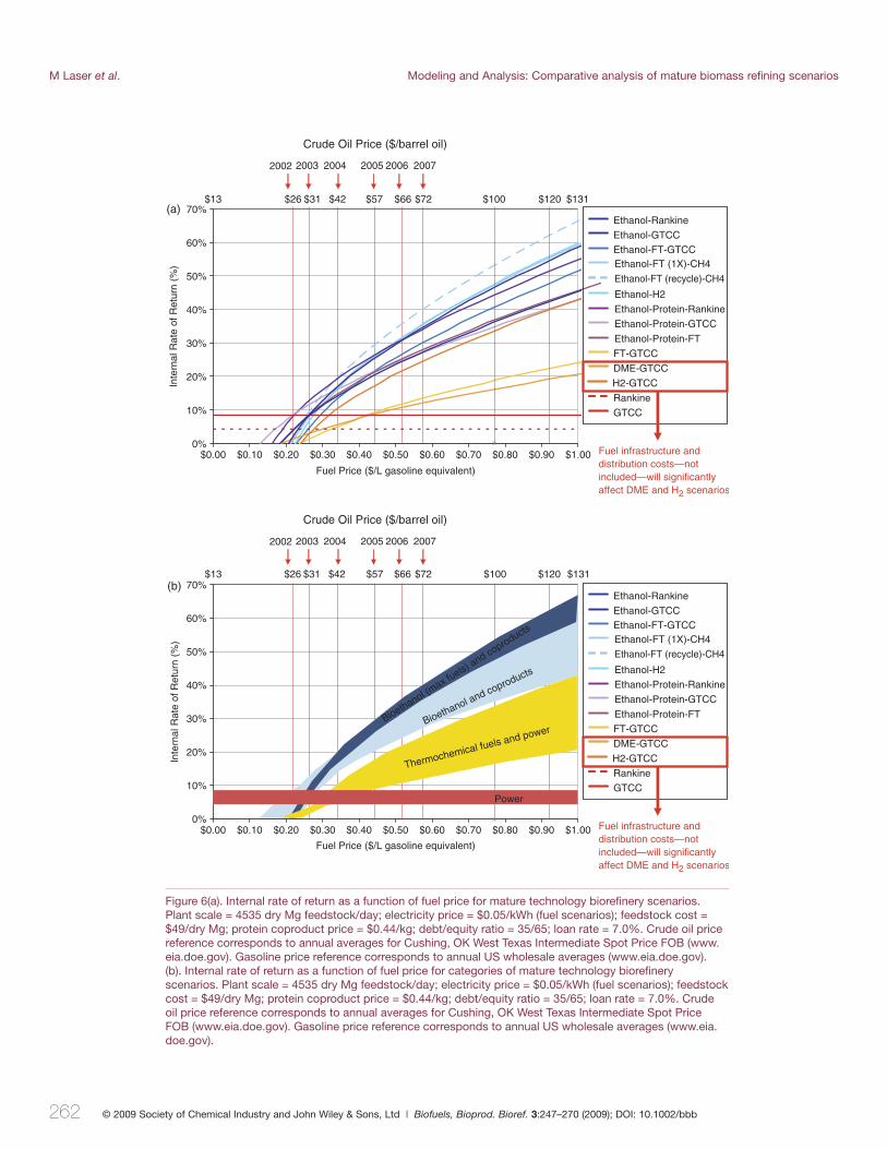
Figures 6(a) and 6(b) present internal rate of return as a
function of fuel price for the mature technology biorefi nery
scenarios at a plant scale of 4535 dry Mgs/day and electricity
price of $0.05/kWh – the approximate average US industrial
price over the last 10 years (www.eia.doe.gov). Th e fi gures
0%
-10%
-20%
-30%
-40%
-50%
-60%
-70%
-80%
-90%
-100%
Per
cent
Cha
nge
Fro
m B
ase
Cas
e
EtO
H/R
anki
ne
EtO
H/G
TC
C
EtO
H/F
T/G
TC
C
EtO
H/F
T/F
T (
1X)/
CH
4
EtO
H/F
T/F
T (
recy
cle)
/CH
4
EtO
H/H
2/G
TC
C
EtO
H/P
rote
in/R
anki
ne
EtO
H/P
rote
in/G
TC
C
EtO
H/P
rote
in/F
T
FT
/GT
CC
DM
E/G
TC
C
H2/
GT
CC
CO2 emissions (gasoline base case = 364 g/km)Petroleum use (gasoline base case = 4.3 MJ/km)
Figure 4. Field-to-wheel CO2 emissions and petroleum use for mature biorefi nery scenarios relative to a conventional gasoline base case. Vehicle effi ciency is 8.33 km/L (19.6 miles/gallon); base case emissions are 349 g CO2/km; base case petroleum use is 4.31 MJ/km.39
© 2009 Society of Chemical Industry and John Wiley & Sons, Ltd | Biofuels, Bioprod. Bioref. 3:247–270 (2009); DOI: 10.1002/bbb 259
Modeling and Analysis: Comparative analysis of mature biomass refining scenarios M Laser et al.
also indicate the annual averages for US crude and gasoline
wholesale prices from 2002 to 2006 (annual averages for
Cushing, OK, West Texas Intermediate crude spot price
FOB). As would be expected, the internal rate of return
(IRR) for the dedicated power scenarios remains constant
as a function of fuel price, with the Rankine and GTCC
scenarios realizing 4.3 and 8.4 %, respectively, while IRR
increases with fuel price for the fuels scenarios. Th e dedi-
cated thermochemical scenarios producing F-T fuels/GTCC
power and DME/GTCC power achieve greater than 10% IRR
at a fuel prices of $0.46 and $0.49/L GEq ($1.76 and $1.85/
gallon), respectively. At $0.79/L GEq ($3.00/gallon), the IRR
rises to 17% for DME and 19% for F-T fuels. Th e H2/GTCC
power scenario is considerably more profi table, achieving
10% IRR at fuel prices above $0.34/L GEq ($1.27/gallon) and
about 35% at $0.79/L GEq ($3.00/gallon). It must be stressed,
however, that hydrogen as a large-scale transportation fuel
would require huge investments in distribution and end-use
infrastructures – costs that are not included in these results.
Post-production costs for hydrogen would be signifi cantly
larger than for the other fuels evaluated here. According to
Wang et al.,30 for example, it would cost about $1.4 million
to convert a current fi lling station to dispense 189,270 L GEq
per month (50,000 gallons/month). Th ey estimate the fi lling
Biological processing
TC processing
Wastewater treatment
Bioprocess cooling towers
Bioprocess make-up
(a)
(b)
Bioprocess cooling tower losses
WWT bleed
TC process air emissions
Bioprocess air emissions
Process steam
Wastewater
WWT losses
Residue moisture
Feedstock moisture
Condensate return
Blowdown
Recycle to TC processing
Recycle to bioprocess cooling towers
Recycle to bioprocessing
BlowdownTC process
cooling towers
TC process cooling tower losses
Blowdown
TC cooling water
make-up
TC process make-up
TC processing
TC process air emissions
TC Make-up
TC process cooling towers
TC process cooling tower losses
TC cooling waterblowdown
TC cooling water
make-up
TC blowdown
Feedstock moisture
Figure 5(a). Overall water fl ows through biorefi nery scenarios with integrated biological and thermochemical processing. (b). Overall water fl ows through biorefi nery scenarios with stand-alone thermochemical processing.
260 © 2009 Society of Chemical Industry and John Wiley & Sons, Ltd | Biofuels, Bioprod. Bioref. 3:247–270 (2009); DOI: 10.1002/bbb
M Laser et al. Modeling and Analysis: Comparative analysis of mature biomass refining scenariosTa
ble
3a.
Ove
rall
pro
cess
wat
er b
alan
ce a
nd m
ake-
up w
ater
req
uire
men
ts fo
r in
teg
rate
d b
iore
finer
y sc
enar
ios.
Sce
nario
Pet
role
umC
orn
Ther
mo
Str
eam
12
34
56
78
9Fu
els
Eth
anol
Pow
er
In (k
g/hr
)
Bio
pro
cess
mak
e-up
217,
656
217,
862
217,
862
217,
862
217,
862
217,
862
380,
713
380,
713
380,
713
Feed
stoc
k m
oist
ure
47,
421
47,
421
47,
421
47,
421
47,
421
47,
421
47,
241
47,
241
47,
241
TC c
oolin
g w
ater
mak
e-up
139,
189
198,
841
198,
841
198,
841
198,
841
198,
841
139,
189
198,
841
198,
841
TC m
ake-
up 3
1,80
7 2
6,41
6 3
9,64
0 3
1,80
4 6
4,89
8 3
6,44
9 3
0,47
9 2
5,05
6 3
6,79
1
Com
bus
tion
rele
ase
55,
808
55,
808
27,
238
41,
063
7,
652
7,
652
55,
808
55,
808
26,
550
TOTA
L49
1,88
154
6,34
853
1,00
253
6,99
053
6,67
450
8,22
565
3,42
970
7,65
869
0,13
6
Out
(kg/
hr)
Bio
pro
cess
em
issi
ons
1,
635
1,
635
1,
635
1,
635
1,
635
1,
635
23,
569
23,
569
23,
569
TC e
mis
sion
s 8
1,71
4 8
1,71
4 6
6,36
9 7
2,35
7 7
2,04
0 4
3,59
1 8
3,89
1 8
3,89
1 6
6,36
9
WW
T b
leed
65,
975
66,
007
66,
007
66,
007
66,
007
66,
007
62,
290
62,
290
62,
290
WW
T lo
sses
1,
041
1,
047
1,
047
1,
047
1,
047
1,
047
9
91
991
9
91
Bio
coo
ling
tow
er lo
sses
200,
290
200,
480
200,
480
200,
480
200,
480
200,
480
343,
473
343,
473
343,
473
TC c
oolin
g w
ater
loss
es12
6,53
518
0,76
418
0,76
418
0,76
418
0,76
518
0,76
412
6,53
518
0,76
418
0,76
4
Hyd
roly
sis
cons
ump
tion
14,
690
14,
700
14,
700
14,
700
14,
700
14,
700
12,
680
12,
680
12,
680
TOTA
L 49
1,88
154
6,34
853
1,00
253
6,99
053
6,67
450
8,22
565
3,42
970
7,65
869
0,13
6
Mak
e-up
(L/L
gas
olin
e eq
uiva
lent
)
Bio
pro
cess
3.98
3.
98
3.98
3.
98
3.98
3.
98
7.52
7.
52
7.52
TC p
roce
ss
22.
94 2
0.14
13.
78 1
0.15
10.
21 1
0.37
83.
32 2
7.98
22.
23
TOTA
L
6.25
6.
43
6.46
5.
79
5.98
5.
85 1
0.45
9.
95
9.62
1.75
a7.
19b
15.8
4c
Coo
ling
wat
er (%
of
tota
l)
84%
86
%
84%
85
%
79%
84
%
85%
87
%
85%
a Sou
rce:
Ref
. 20.
b S
ourc
e: R
ef. 1
8.c S
ourc
e: R
ef. 2
2.
© 2009 Society of Chemical Industry and John Wiley & Sons, Ltd | Biofuels, Bioprod. Bioref. 3:247–270 (2009); DOI: 10.1002/bbb 261
Modeling and Analysis: Comparative analysis of mature biomass refining scenarios M Laser et al.
Tab
le 3
b. O
vera
ll p
roce
ss w
ater
bal
ance
and
mak
e-up
wat
er r
equi
rem
ents
for
ded
icat
ed t
herm
och
emic
al fu
els
and
po
wer
sce
nari
os.
Sce
nario
Pet
role
umC
orn
Ther
mo
Str
eam
1011
1213
14Fu
els
Eth
anol
Pow
erIn
(kg/
hr)
TC m
ake-
up11
0,45
558
,150
91,1
2648
,965
48,9
65
Feed
stoc
k m
oist
ure
47,4
2147
,421
47,4
2147
,421
47,4
21
TC c
oolin
g w
ater
mak
e-up
720,
201
720,
201
720,
201
504,
141
720,
201
Com
bus
tion
rele
ase
98,6
5683
,520
83,1
6010
6,03
410
6,03
4
TOTA
L97
6,73
390
9,29
294
1,90
870
6,56
192
2,62
1
Out
(kg/
hr)
TC e
mis
sion
s24
0,38
517
2,94
420
5,56
018
6,27
318
6,27
3
TC b
low
dow
n16
,147
16,1
4716
,147
16,1
4716
,147
TC c
oolin
g w
ater
loss
es65
4,72
965
4,72
965
4,72
945
8,31
065
4,72
9
TC c
oolin
g w
ater
blo
wd
own
65,4
7365
,473
65,4
7345
,831
65,4
73
TOTA
L 97
6,73
390
9,29
294
1,90
870
6,56
192
2,62
1
Mak
e-up
(L/L
gas
olin
e eq
uiv.
)14
.23
14.1
312
.55
16.6
815
.24
1.75
a7.
19b
15.8
4c
Coo
ling
wat
er (%
of t
otal
)87
%
93%
89
%
91%
94
%a S
ourc
e: R
ef. 2
0.b S
ourc
e: R
ef. 1
8.c S
ourc
e: R
ef. 2
2.
262 © 2009 Society of Chemical Industry and John Wiley & Sons, Ltd | Biofuels, Bioprod. Bioref. 3:247–270 (2009); DOI: 10.1002/bbb
M Laser et al. Modeling and Analysis: Comparative analysis of mature biomass refining scenarios
0%
10%
20%
30%
40%
50%
60%
70%(a)
(b)
$0.00 $0.10 $0.20 $0.30 $0.40 $0.50 $0.60 $0.70 $0.80 $0.90 $1.00
Fuel Price ($/L gasoline equivalent)
Inte
rnal
Rat
e of
Ret
urn
(%)
Rankine
GTCC
Ethanol-FT-GTCCEthanol-FT (1X)-CH4
Ethanol-FT (recycle)-CH4
Ethanol-H2
Ethanol-Protein-Rankine
Ethanol-Protein-GTCC
Ethanol-Protein-FT
Ethanol-GTCC
Ethanol-Rankine
FT-GTCC
DME-GTCC
H2-GTCC
$26 $31 $42 $57 $66 $72 $100 $120
2002 2003 2004 2005 2006 2007
$13
Crude Oil Price ($/barrel oil)
Fuel infrastructure and distribution costs—not included—will significantly affect DME and H2 scenarios
$131
0%
10%
20%
30%
40%
50%
60%
70%
$0.00 $0.10 $0.20 $0.30 $0.40 $0.50 $0.60 $0.70 $0.80 $0.90 $1.00
Fuel Price ($/L gasoline equivalent)
Inte
rnal
Rat
e of
Ret
urn
(%)
Bioethanol (max fu
els) and coproducts
Bioethanol and coproducts
Thermochemical fuels and power
Power
Figure 6(a). Internal rate of return as a function of fuel price for mature technology biorefi nery scenarios. Plant scale = 4535 dry Mg feedstock/day; electricity price = $0.05/kWh (fuel scenarios); feedstock cost = $49/dry Mg; protein coproduct price = $0.44/kg; debt/equity ratio = 35/65; loan rate = 7.0%. Crude oil price reference corresponds to annual averages for Cushing, OK West Texas Intermediate Spot Price FOB (www.eia.doe.gov). Gasoline price reference corresponds to annual US wholesale averages (www.eia.doe.gov). (b). Internal rate of return as a function of fuel price for categories of mature technology biorefi nery scenarios. Plant scale = 4535 dry Mg feedstock/day; electricity price = $0.05/kWh (fuel scenarios); feedstock cost = $49/dry Mg; protein coproduct price = $0.44/kg; debt/equity ratio = 35/65; loan rate = 7.0%. Crude oil price reference corresponds to annual averages for Cushing, OK West Texas Intermediate Spot Price FOB (www.eia.doe.gov). Gasoline price reference corresponds to annual US wholesale averages (www.eia.doe.gov).
© 2009 Society of Chemical Industry and John Wiley & Sons, Ltd | Biofuels, Bioprod. Bioref. 3:247–270 (2009); DOI: 10.1002/bbb 263
Modeling and Analysis: Comparative analysis of mature biomass refining scenarios M Laser et al.
station conversion cost for ethanol and DME at $200,000,
and minimal costs for F-T diesel. James and Perez 31estimate
infrastructure (terminal construction and dispensing) and
distributions costs for hydrogen produced via switchgrass
gasifi cation at about $0.40/L GEq ($1.50/gallon), which
would roughly double the costs presented here.
Th e most profi table scenarios all involve biological
processing of the feedstock carbohydrate fraction, achieving
10% IRR at fuel prices ranging from $0.24 to $0.31/L GEq
($0.89 to $1.16/gallon) depending on the scenario, and rising
to 36%–54% at $0.79/L GEq ($3.00/gallon). At fuel prices
of $0.26/L GEq ($1.00/gallon) – or about $30/barrel oil
– the dedicated thermochemical fuels scenarios have IRRs
less than 5%, while the two biological scenarios involving
protein coproduction and power remain profi table with the
ethanol-protein-GTCC-power scenario achieving about 12%,
and the ethanol-protein-Rankine power realizing 14%. At
the historical low soy meal protein price from 1980 to 2006
– about $0.31/kg, as noted in Laser et al.5 – the fuel price for
the ethanol-protein-Rankine confi guration is $0.19/L, equal
to the break-even price (i.e., the point at which the price is
equal to that for the same confi guration without protein
coproduction). At the historical high ($0.62/kg), the fuel
$0.02 $0.04 $0.06 $0.08 $0.10 $0.12 $0.14
Electricity Price ($/kWh)
0%
5%
10%
15%
20%
25%
30%
35%
40%
$5 $10 $15 $20 $25 $30 $35 $40
Electricity Price ($/GJ )
Inte
rnal
Rat
e of
Ret
urn
(%)
Bioethanol and coproducts
TC Fuels and power
Power
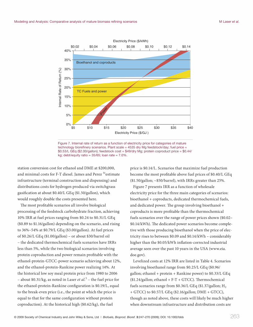
Figure 7. Internal rate of return as a function of electricity price for categories of mature technology biorefi nery scenarios. Plant scale = 4535 dry Mg feedstock/day; fuel price = $0.53/L GEq ($2.00/gallon); feedstock cost = $49/dry Mg; protein coproduct price = $0.44/kg; debt/equity ratio = 35/65; loan rate = 7.0%.
price is $0.14/L. Scenarios that maximize fuel production
become the most profi table above fuel prices of $0.40/L GEq
($1.50/gallon; ~$50/barrel), with IRRs greater than 25%.
Figure 7 presents IRR as a function of wholesale
electricity price for the three main categories of scenarios:
bioethanol + coproducts, dedicated thermochemical fuels,
and dedicated power. Th e group involving bioethanol +
coproducts is more profi table than the thermochemical
fuels scenarios over the range of power prices shown ($0.02–
$0.14/kWh). Th e dedicated power scenarios become comple-
tive with those producing bioethanol when the price of elec-
tricity rises to between $0.09 and $0.14/kWh – considerably
higher than the $0.05/kWh infl ation-corrected industrial
average seen over the past 10 years in the USA (www.eia.
doe.gov).
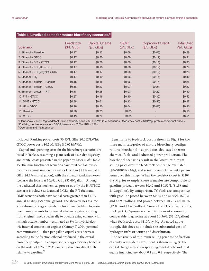
Levelized costs at 12% IRR are listed in Table 4. Scenarios
involving bioethanol range from $0.25/L GEq ($0.96/
gallon; ethanol + protein + Rankine power) to $0.33/L GEq
($1.24/gallon; ethanol + F-T + GTCC). Th ermochemical
fuels scenarios range from $0.36/L GEq ($1.37/gallon; H2
+ GTCC) to $0.57/L GEq ($2.16/gallon; DME + GTCC),
though as noted above, these costs will likely be much higher
when downstream infrastructure and distribution costs are
264 © 2009 Society of Chemical Industry and John Wiley & Sons, Ltd | Biofuels, Bioprod. Bioref. 3:247–270 (2009); DOI: 10.1002/bbb
M Laser et al. Modeling and Analysis: Comparative analysis of mature biomass refining scenarios
included. Rankine power costs $0.55/L GEq ($0.062/kWh);
GTCC power costs $0.51/L GEq ($0.058/kWh).
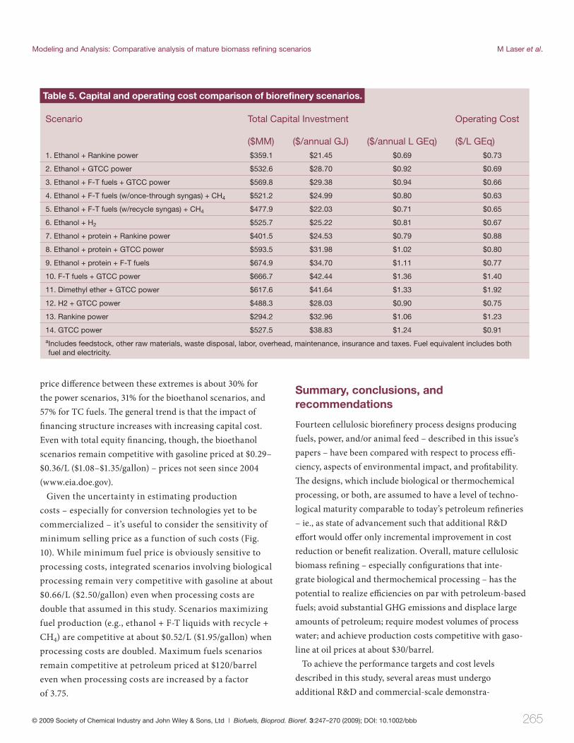
Capital and operating costs for the biorefi nery scenarios are
listed in Table 5, assuming a plant scale of 4535 dry Mgs/day
and capital costs presented in the paper by Laser et al.5 Table
15. Th e nine bioethanol scenarios have total capital invest-
ment per annual unit energy values less than $1.12/annual L
GEq ($4.25/annual gallon), with the ethanol-Rankine-power
scenario the lowest at $0.69/L GEq ($2.60/gallon). Among
the dedicated thermochemical processes, only the H2/GTCC
scenario is below $1.12/annual L GEq; the F-T fuels and
DME scenarios both have capital costs greater than $1.32/
annual L GEq ($5/annual gallon). Th e above values assume
a one-to-one energy equivalence for ethanol relative to gaso-
line. If one accounts for potential effi ciency gains resulting
from engines tuned specifi cally to operate using ethanol with
its high octane number – estimated as 8% for hybrid elec-
tric internal combustion engines (Kenney T, 2004, personal
communication) – then per-gallon capital costs decrease
according to the fraction ethanol produced in the overall
biorefi nery output. In comparison, energy effi ciency benefi ts
on the order of 15% to 25% can be realized for diesel fuels
relative to gasoline.32
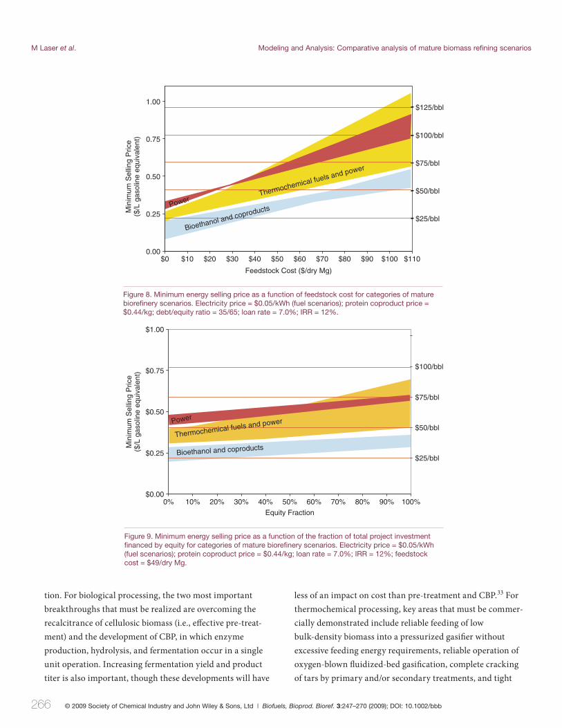
Sensitivity to feedstock cost is shown in Fig. 8 for the
three main categories of mature biorefinery configu-
rations: bioethanol + coproducts, dedicated thermo-
chemical fuels, and dedicated power production. The
bioethanol scenarios result in the lowest minimum
selling price over the feedstock cost range evaluated
($0–$100/dry Mg), and remain competitive with petro-
leum over this range. When the feedstock cost is $110/
dry Mg, for example, these scenarios are comparable to
gasoline priced between $0.42 and $0.52/L ($1.58 and
$1.98/gallon). By comparison, TC fuels are competitive
with gasoline priced between $0.56 and $1.05/L ($2.12
and $3.99/gallon); and power, between $0.75 and $0.91/L
($2.83 and $3.45/gallon). Among the TC configurations,
the H2-GTCC-power scenario is the most economic,
comparable to gasoline at about $0.56/L ($2.12/gallon)
when feedstock costs $110/dry Mg. As noted above,
though, this does not include the substantial cost of
hydrogen infrastructure and distribution.
Th e sensitivity of minimum selling price to the fraction
of equity versus debt investment is shown in Fig. 9. Th e
capital charge rates corresponding to total debt and total
equity fi nancing are about 0.1 and 0.2, respectively. Th e
Table 4. Levelized costs for mature biorefinery scenarios.a
ScenarioFeedstock ($/L GEq)
Capital Charge ($/L GEq)
O&Mb ($/L GEq)
Coproduct Credit ($/L GEq)
Total Cost($/L GEq)
1. Ethanol + Rankine $0.17 $0.12 $0.06 ($0.06) $0.29
2. Ethanol + GTCC $0.17 $0.20 $0.06 ($0.12) $0.31
3. Ethanol + F-T + GTCC $0.17 $0.20 $0.06 ($0.11) $0.33
4. Ethanol + F-T (1X) + CH4 $0.17 $0.18 $0.06 ($0.12) $0.29
5. Ethanol + F-T (recycle) + CH4 $0.17 $0.17 $0.06 ($0.12) $0.28
6. Ethanol + H2 $0.17 $0.19 $0.06 ($0.11) $0.30
7. Ethanol + protein + Rankine $0.18 $0.15 $0.06 ($0.14) $0.25
8. Ethanol + protein + GTCC $0.18 $0.23 $0.07 ($0.21) $0.27
9. Ethanol + protein + F-T $0.18 $0.25 $0.07 ($0.20) $0.30
10. F-T + GTCC $0.27 $0.46 $0.10 ($0.30) $0.52
11. DME + GTCC $0.38 $0.61 $0.13 ($0.55) $0.57
12. H2 + GTCC $0.16 $0.20 $0.04 ($0.03) $0.36
13. Rankine $0.28 $0.23 $0.05 - $0.56
14. GTCC $0.19 $0.27 $0.05 - $0.51aPlant scale = 4535 Mg feedstock/day; electricity price = $0.05/kWh (fuel scenarios); feedstock cost = $49/Mg; protein coproduct price = $0.44/kg; debt/equity ratio = 35/65; loan rate = 7.0%; IRR = 12%.bOperating and maintenance.
© 2009 Society of Chemical Industry and John Wiley & Sons, Ltd | Biofuels, Bioprod. Bioref. 3:247–270 (2009); DOI: 10.1002/bbb 265
Modeling and Analysis: Comparative analysis of mature biomass refining scenarios M Laser et al.
price diff erence between these extremes is about 30% for
the power scenarios, 31% for the bioethanol scenarios, and
57% for TC fuels. Th e general trend is that the impact of
fi nancing structure increases with increasing capital cost.
Even with total equity fi nancing, though, the bioethanol
scenarios remain competitive with gasoline priced at $0.29–
$0.36/L ($1.08–$1.35/gallon) – prices not seen since 2004
(www.eia.doe.gov).
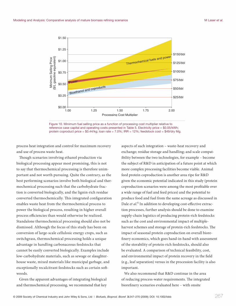
Given the uncertainty in estimating production
costs – especially for conversion technologies yet to be
commercialized – it’s useful to consider the sensitivity of
minimum selling price as a function of such costs (Fig.
10). While minimum fuel price is obviously sensitive to
processing costs, integrated scenarios involving biological
processing remain very competitive with gasoline at about
$0.66/L ($2.50/gallon) even when processing costs are
double that assumed in this study. Scenarios maximizing
fuel production (e.g., ethanol + F-T liquids with recycle +
CH4) are competitive at about $0.52/L ($1.95/gallon) when
processing costs are doubled. Maximum fuels scenarios
remain competitive at petroleum priced at $120/barrel
even when processing costs are increased by a factor
of 3.75.
Summary, conclusions, and recommendations
Fourteen cellulosic biorefi nery process designs producing
fuels, power, and/or animal feed – described in this issue’s
papers – have been compared with respect to process effi -
ciency, aspects of environmental impact, and profi tability.
Th e designs, which include biological or thermochemical
processing, or both, are assumed to have a level of techno-
logical maturity comparable to today’s petroleum refi neries
– ie., as state of advancement such that additional R&D
eff ort would off er only incremental improvement in cost
reduction or benefi t realization. Overall, mature cellulosic
biomass refi ning – especially confi gurations that inte-
grate biological and thermochemical processing – has the
potential to realize effi ciencies on par with petroleum-based
fuels; avoid substantial GHG emissions and displace large
amounts of petroleum; require modest volumes of process
water; and achieve production costs competitive with gaso-
line at oil prices at about $30/barrel.
To achieve the performance targets and cost levels
described in this study, several areas must undergo
additional R&D and commercial-scale demonstra-
Table 5. Capital and operating cost comparison of biorefinery scenarios.
Scenario Total Capital Investment Operating Cost
($MM) ($/annual GJ) ($/annual L GEq) ($/L GEq)1. Ethanol + Rankine power $359.1 $21.45 $0.69 $0.73
2. Ethanol + GTCC power $532.6 $28.70 $0.92 $0.69
3. Ethanol + F-T fuels + GTCC power $569.8 $29.38 $0.94 $0.66
4. Ethanol + F-T fuels (w/once-through syngas) + CH4 $521.2 $24.99 $0.80 $0.63
5. Ethanol + F-T fuels (w/recycle syngas) + CH4 $477.9 $22.03 $0.71 $0.65
6. Ethanol + H2 $525.7 $25.22 $0.81 $0.67
7. Ethanol + protein + Rankine power $401.5 $24.53 $0.79 $0.88
8. Ethanol + protein + GTCC power $593.5 $31.98 $1.02 $0.80
9. Ethanol + protein + F-T fuels $674.9 $34.70 $1.11 $0.77
10. F-T fuels + GTCC power $666.7 $42.44 $1.36 $1.40
11. Dimethyl ether + GTCC power $617.6 $41.64 $1.33 $1.92
12. H2 + GTCC power $488.3 $28.03 $0.90 $0.75
13. Rankine power $294.2 $32.96 $1.06 $1.23
14. GTCC power $527.5 $38.83 $1.24 $0.91a Includes feedstock, other raw materials, waste disposal, labor, overhead, maintenance, insurance and taxes. Fuel equivalent includes both fuel and electricity.
266 © 2009 Society of Chemical Industry and John Wiley & Sons, Ltd | Biofuels, Bioprod. Bioref. 3:247–270 (2009); DOI: 10.1002/bbb
M Laser et al. Modeling and Analysis: Comparative analysis of mature biomass refining scenarios
tion. For biological processing, the two most important
breakthroughs that must be realized are overcoming the
recalcitrance of cellulosic biomass (i.e., eff ective pre-treat-
ment) and the development of CBP, in which enzyme
production, hydrolysis, and fermentation occur in a single
unit operation. Increasing fermentation yield and product
titer is also important, though these developments will have
less of an impact on cost than pre-treatment and CBP.33 For
thermochemical processing, key areas that must be commer-
cially demonstrated include reliable feeding of low
bulk-density biomass into a pressurized gasifi er without
excessive feeding energy requirements, reliable operation of
oxygen-blown fl uidized-bed gasifi cation, complete cracking
of tars by primary and/or secondary treatments, and tight
$25/bbl
$50/bbl
$75/bbl
$100/bbl
$125/bbl
Bioethanol and coproducts
Thermochemical fuels and power
Power
0.00
0.25
0.50
0.75
1.00
$0 $10 $20 $30 $40 $50 $60 $70 $80 $90 $100 $110
Feedstock Cost ($/dry Mg)
Min
imum
Sel
ling
Pric
e ($
/L g
asol
ine
equi
vale
nt)
Figure 8. Minimum energy selling price as a function of feedstock cost for categories of mature biorefi nery scenarios. Electricity price = $0.05/kWh (fuel scenarios); protein coproduct price = $0.44/kg; debt/equity ratio = 35/65; loan rate = 7.0%; IRR = 12%.
$25/bbl
$50/bbl
$75/bbl
$100/bbl
$0.00
$0.25
$0.50
$0.75
$1.00
0% 10% 20% 30% 40% 50% 60% 70% 80% 90% 100%
Equity Fraction
Min
imum
Sel
ling
Pric
e ($
/L g
asol
ine
equi
vale
nt)
Bioethanol and coproducts
Thermochemical fuels and powerPower
Figure 9. Minimum energy selling price as a function of the fraction of total project investment fi nanced by equity for categories of mature biorefi nery scenarios. Electricity price = $0.05/kWh (fuel scenarios); protein coproduct price = $0.44/kg; loan rate = 7.0%; IRR = 12%; feedstock cost = $49/dry Mg.
© 2009 Society of Chemical Industry and John Wiley & Sons, Ltd | Biofuels, Bioprod. Bioref. 3:247–270 (2009); DOI: 10.1002/bbb 267
Modeling and Analysis: Comparative analysis of mature biomass refining scenarios M Laser et al.
process heat integration and control for maximum recovery
and use of process waste heat.
Th ough scenarios involving ethanol production via
biological processing appear most promising, this is not
to say that thermochemical processing is therefore unim-
portant and not worth pursuing. Quite the contrary, as the
best performing scenarios involve both biological and ther-
mochemical processing such that the carbohydrate frac-
tion is converted biologically, and the lignin-rich residue
converted thermochemically. Th is integrated confi guration
enables waste heat from the thermochemical process to
power the biological process, resulting in higher overall
process effi ciencies than would otherwise be realized.
Standalone thermochemical processing should also not be
dismissed. Although the focus of this study has been on
conversion of large-scale cellulosic energy crops, such as
switchgrass, thermochemical processing holds a unique
advantage in handling carbonaceous feedstocks that
cannot be easily converted biologically. Examples include
low-carbohydrate materials, such as sewage or slaughter-
house waste, mixed materials like municipal garbage, and
exceptionally recalcitrant feedstocks such as certain soft -
woods.
Given the apparent advantages of integrating biological
and thermochemical processing, we recommend that key
aspects of such integration – waste-heat recovery and
exchange; residue storage and handling; and scale compat-
ibility between the two technologies, for example – become
the subject of R&D in anticipation of a future point at which
more complex processing facilities become viable. Animal
feed protein coproduction is another area ripe for R&D
given the economic potential indicated in this study (protein
coproduction scenarios were among the most profi table over
a wide range of fuel and feed prices) and the potential to
produce food and fuel from the same acreage as discussed in
Dale et al.6 In addition to developing cost-eff ective extrac-
tion processes, further analysis should be done to examine
supply-chain logistics of producing protein-rich feedstocks
such as the cost and environmental impact of multiple-
harvest schemes and storage of protein-rich feedstocks. Th e
impact of seasonal protein coproduction on overall biore-
fi nery economics, which goes hand-in-hand with assessment
of the storability of protein-rich feedstocks, should also
be evaluated. A comparison of technical feasibility, cost,
and environmental impact of protein recovery in the fi eld
(e.g., leaf separation) versus in the procession facility is also
important.
We also recommend that R&D continue in the area
of reducing process-water requirements. Th e integrated
biorefi nery scenarios evaluated here – with onsite
$25/bbl
$50/bbl
$75/bbl
$100/bbl
$125/bbl
$150/bbl
$0.00
$0.25
$0.50
$0.75
$1.00
$1.25
$1.50
1.00 1.25 1.50 1.75 2.00Processing Cost Multiplier
Min
imum
Sel
ling
Pric
e ($
/L g
asol
ine
equi
vale
nt)
Bioethanol and coproducts
Thermochemical fuels and power
Power
Figure 10. Minimum fuel selling price as a function of processing cost multiplier relative to reference case capital and operating costs presented in Table 5. Electricity price = $0.05/kWh; protein coproduct price = $0.44/kg; loan rate = 7.0%; IRR = 12%; feedstock cost = $49/dry Mg.

268 © 2009 Society of Chemical Industry and John Wiley & Sons, Ltd | Biofuels, Bioprod. Bioref. 3:247–270 (2009); DOI: 10.1002/bbb
M Laser et al. Modeling and Analysis: Comparative analysis of mature biomass refining scenarios
waste-water treatment and extensive recycle – have been
designed with an eye toward reducing make-up water.
Scenarios involving protein coproduction and standalone
thermochemical processing, however, were not optimized
with respect to water demand. In all scenarios, signifi cant
amounts are lost through evaporation in cooling towers.
Reducing these losses through innovations, such as forced-
air cooling and the HiCycler process – a sidestream hard-
ness and silica removal process that reduces blowdown by
95% (http://www.chemico.com/HiCycler.htm) – would
greatly improve the process-water balance. Development
and evaluation of process designs incorporating such inno-
vations would be a useful contribution. We also recommend
that water pinch analysis be performed on these designs
to elucidate further opportunities for more effi cient water
use. Water pinch analysis has been used predominantly
in the food processing industry to great eff ect, with some
reports of make-up water reductions of up to 50%.34 While
reducing process-water demand is an important goal,
we note that when the entire lifecycle is considered for
corn ethanol, signifi cantly more water is consumed in the
fi eld during the growth of the corn than in the dry mill
– between 75 and 895 L water/kg corn (500–6000 gallon
water/bushel) depending on geographic location, or about
175–2140 L water/L ethanol.27 (Again, more recent analysis
by Wu and Wang28 suggests that actual consumed water
is much lower – 7.1 to 320.6 L water/L ethanol.) Th is is
also likely to be the case for cellulosic biofuels. Research
is underway, however, to identify and develop cellulosic
energy crops that require less water than corn while
achieving comparable if not greater biomass yields.35–37
Such eff orts, if successful, will profoundly contribute to the
sustainability of biofuels.
Th ough the RBAEF project has examined many poten-
tial biorefi nery scenarios, the eff ort has by no means been
exhaustive; the project’s encouraging results suggest analysis
of additional technologies and process confi gurations, such
as pyrolysis, liquefaction, syngas fermentation, and concen-
trated acid hydrolysis may also be fruitful and informative.
In addition, a more extensive fi eld-to-wheels lifecycle assess-
ment that incorporates the RBAEF process design results
– including a comparison of alternative feedstocks – would
be useful, as would an evaluation of chemicals coproduction.
Also, we recommend a more comprehensive analysis of the
eff ect on carbon emissions of land conversion to biofuels than
currently available in the literature. Finally, having sketched a
picture of mature biomass refi ning – one having potential to
contribute signifi cantly to demand for energy services in the
USA – it would be of great value to assess possible transition
pathways to help streamline progress toward this promising
and sustainable future.
Acknowledgements
We thank all of our colleagues in the RBAEF project for
stimulating and informative discussions throughout the
course of the project, which contributed directly and
indirectly to the contents of this paper: David Bransby,
Fuat Celik, Kemantha Jayawardhana, Haiming Jin, Jim
Kiniry, Amit Kumar Sudhagar Mani, John McBride,
Samuel McLaughlin, Steve Peterson, Daniel Saccardi, John
Sheehan, Shahab Sokhansanj, Charles Taliaferro, Anthony
Turhollow, Daniel Ugarte, May Wu, Charles Wyman. We
also acknowledge other colleagues who also off ered their
judgment, information, and assistance: Andy Aden, Michael
Casler, Gordon Cheng, Joel Cherry, Billie Christen, Patrick
Costello, John DeCicco, Reid Detchon, Tim Eggeman,
Alison Findon, David Friedman, John German, Tillman
Gerngross, Robin Graham, Chad Hellwinckel, Bob Hickey,
Martin Hocking, Kelly Ibsen, John Jechura, Hans Jung,
Tom Kenney, Drew Kodjak, Jason Mark, Roger McDaniel,
William Mitchell, Joan Ogden, Michael Pacheco, Charlotte
Pera, Srini Raj, Lloyd Ritter, Larry Russo, Mark Ruth, Daniel
Santini, Pamela Spath, Richard Tolman, Ken Vogel, and
Luca Zullo. For fi nancial support, we thank the National
Renewable Energy Laboratory (award #: XCO-3-33033-01),
the National Institute of Standards and Technology (award
#: 60NANB1D0064), and the National Science Foundation
(award #: CMS – 0424700).
References 1. Lynd LR, Larson ED, Greene N, Laser M, Sheehan J, Dale BE,
McLaughlin S and Wang M, The role of biomass in America’s energy
future: framing the analysis. Biofuels, Bioprod. Bioref. 3:113–123 (2009).
2. Sokhansanj S, Mani S, Turhollow A, Kumar A, Bransby D, Lynd L and
Laser M, Large scale production, harvest and transport of switchgrass
(Panicum virgatum L.) – current technology and visioning a mature
technology. Biofuels, Bioprod. Bioref. 3:124–141 (2009).
© 2009 Society of Chemical Industry and John Wiley & Sons, Ltd | Biofuels, Bioprod. Bioref. 3:247–270 (2009); DOI: 10.1002/bbb 269
Modeling and Analysis: Comparative analysis of mature biomass refining scenarios M Laser et al.
3. Jin H, Larson ED and Celik FE, Performance and cost analysis of future,
commercially mature gasifi cation-based electric power generation from
switchgrass. Biofuels, Bioprod. Bioref. 3:142–173 (2009).
4. Larson ED, Jin H and Celik FE, Large-scale gasifi cation-based
coproduction of fuels and electricity from switchgrass. Biofuels, Bioprod.
Bioref. 3:174–194 (2009).
5. Laser M, Jin H, Jayawardhana K and Lynd LR, Coproduction of ethanol
and power from switchgrass. Biofuels, Bioprod. Bioref. 3:195–218 (2009).
6. Dale BE, Allen MS, Laser M and Lynd LR, Protein feeds coproduction in
biomass conversion to fuels and chemicals. Biofuels, Bioprod. Bioref.
3:219–230 (2009).
7. Laser M, Jin H, Jayawardhana K, Dale BE and Lynd LR, Projected mature
technology scenarios for conversion of cellulosic biomass to ethanol with
coproduction thermochemical fuels, power, and/or animal feed protein.
Biofuels, Bioprod. Bioref. 3:231–246 (2009).
8. So KS and Brown RC, Economic analysis of selected lignocellulose-to-
ethanol conversion technologies. Appl Biochem Biotechnol 77–79:
633–640 (1999).
9. Wright MM and Brown RC, Comparative economics of biorefi neries
based on the biochemical and thermochemical platforms. Biofuels,
Bioprod. Bioref. 1:49–56 (2007).
10. Piccolo C and Bezzo F, A techno-economic comparison between two
technologies for bioethanol production from lignocellulose. Biomass
Bioenerg DOI:10.1016/j.biombioe.2008.08.008 (2009).
11. Shapouri H, Duffi eld JA and Wang M, The energy balance of corn
ethanol: an update. US Department of Agriculture (2002).
12. Searchinger T, Heimlich R, Houghton RA, Dong F, Elobeid A, Fabiosa
J, Tokgoz S, Hayes D and Yu T-H, Use of US croplands for biofuels
increases greenhouse gases through emissions from land use change.
Science 319:1238–1240 (2008).
13. Fargione J, Hill J, Tilman D, Polasky S and Hawthorne P, Land clearing
and the biofuel carbon debt. Science 319:1235–1238 (2008).
14. Wu M, Wu Y and Wang M, Energy and emission benefi ts of alternative
transportation liquid fuels derived from switchgrass: a fuel life cycle
assessment. Biotechnol Progr 22:1012–1024 (2006).
15. Kutscher CF (ed.), Tackling climate change in the US, American Solar
Energy Society: Boulder, CO (2007).
16. Hedegaard K, Thyø KA and Wenzel H, Life cycle assessment of an
advanced bioethanol technology in the perspective of constrained
biomass availability. Environ Sci Technol 42:7992–7999 (2008).
17. Energy Information Administration, Annual Energy Outlook 2009: Early
Release. (www.eia.doe.gov) (2009).
18. Pate R, Hightower M, Cameron C and Einfeld W, Overview of energy-
water interdependencies and the emerging energy demands on water
resources. Report SAND 2007-1349C; Sandia National Laboratories, Los
Alamos, NM (2007).
19. Wallace R, Ibsen K, McAloon A and Lee W, Feasibility study for co-
locating and integrating ethanol production plants from corn starch
and lignocellulosic feedstocks. National Renewable Energy Laboratory
(NREL/TP-510-37092) and United States Department of Agriculture
(USDA-ARS 1935-41000-055-00D) (2005).
20. Gleick PH, Water and energy. Annu Rev Energ Env 19:267–299 (1994).
21. Data for Environmental Analysis and Management (DEAM), Ecobilan, Neuilly-
sur-Seine – France (http://www.ecobalance.com/uk_deam.php) (2007).
22. Torcellini P, Long N and Judkoff R, Consumptive water use for US
power production. NREL/CP-550-35190, National Renewable Energy
Laboratory, Golden, CO (2003).
23. Saville BA, Feasibility study for a biodiesel refi ning facility in the regional
municipality of Durham. BBI Biofuels Canada, Kitchener, ON (2006).
24. Sandy T, Water reduction and reuse in the petroleum industry. Presented
at 69th meeting of the Petroleum Environmental Research Forum;
Annapolis, MD; November 1–4, (2005).
25. Aden A, Water usage for current and future ethanol production.
Southwest Hydrology 6:22–23 (2007).
26. European Commission, Integrated Pollution Prevention and Control.
Reference document on the application of best available techniques to
industrial cooling systems. (2001).
27. National Academy of Sciences, Water Implications of Biofuels Production
in the United States. Committee on Water Implications of Biofuels
Production in the United States, National Research Council; ISBN: 0-
309-11360-1 (2007).
28. Wu M and Wang M, Addressing consumptive water use for sustainable
biofuel development. Presented at BIOMASS 2008, Washington, DC,
April 17 (2008).
29. McLaughlin SB, Kiniry JR, Taliaferro CM and De La Torre Ugarte D,
Projecting yield and utilization potential of switchgrass as an energy
crop. Adv Agron 90:267–296 (2007).
30. Wang M. Mintz M, Singh M, Stork K, Vyas V and Johnson L, Assessment
of PNGV fuels infrastructure, phase 2 – fi nal report: additional capital
needs and fuel cycle energy and emissions impacts. Argonne, IL:
Argonne National Laboratory, Center for Transportation Research and
Decision and Information Sciences Division (1998).
31. James B and Perez J, Hydrogen infrastructure pathways analysis using
HYPRO, in Analysis of the transition to fuel cell vehicles and the potential
hydrogen energy infrastructure requirements, ed by McQueen S. Oak
Ridge National Laboratory, Oak Ridge, TN (2008).
32. Monahan P and Friedman D, The diesel dilemma: diesel’s role in the race
for clean cars. Union of Concerned Scientists; Cambridge, MA (2004).
33. Lynd LR, Laser MS, Bransby D, Dale BE, Davison B, Hamilton R, Himmel
M, Keller M, McMillan JD, Sheehan J and Wyman CE, How biotech can
transform biofuels. Nature Biotechnol 26:169–172 (2008).
34. Polley GT and Polley HL, Design better water networks. Chem Eng Progr
96:47–52 (2000).
35. Condon AG, Richards RA, Rebetzke GJ and Farquhar GD, Breeding for
high water-use effi ciency. J Exp Bot 55:2447–2460 (2004).
36. Wikberg J and Ogren E, Interrelationships between water use and growth
traits in biomass-producing willows. Trees-Struct Funct 18:70–76 (2004).
37. Hatfi eld JL, Sauer TJ and Prueger JH, Managing soils to achieve greater
water use effi ciency: a review. Agron J 96:271–280 (2001).
38. Interlaboratory Working Group. Scenarios for a clean energy future. Oak
Ridge National Laboratory, Oak Ridge, TN; Lawrence Berkeley National
Laboratory, Berkeley, CA; National Renewable Energy Laboratory,
Golden, CO; ORNL/CON-476; LBNL-44029; NREL/TP-620-29379 (2000).
39. Greenhouse Gases, Regulated Emissions, and Energy Use in Transportation
(GREET) Model. Argonne National Laboratory, Argonne, IL (2005).

270 © 2009 Society of Chemical Industry and John Wiley & Sons, Ltd | Biofuels, Bioprod. Bioref. 3:247–270 (2009); DOI: 10.1002/bbb
M Laser et al. Modeling and Analysis: Comparative analysis of mature biomass refining scenarios
Eric D. Larson
Larson is a senior member of the Energy Sys-
tems Analysis Group within the Princeton En-
vironmental Institute and an affiliated faculty
member in Princeton’s Science, Technology,
and Environmental Policy Program. Research
interests include engineering, economic, and
policy-related assessments of advanced
clean-energy systems, especially for electric power and transport
fuels production from carbonaceous fuels (biomass, coal, natural
gas) and for efficient end use of energy. He was the task leader for
thermochemical conversion technologies in the RBAEF
project.
Nathanael Greene
Nathanael Greene is the Director of Renew-
able Energy Policy at NRDC and is respon-
sible for coordinating work on renewable
fuels and power. With particular expertise in
clean energy technologies, he also works on
broader energy policy including utility restruc-
turing, energy taxes, energy efficiency, and
low-income services. He has been focusing recently on assessing
the sustainable potential for biofuels and developing policies to
advance them.
Mark Laser
Mark Laser is a research scientist and lec-
turer at the Thayer School of Engineering,
Dartmouth College. As an analyst and project
manager in the area of conversion of cel-
lulosic biomass to fuels and other products,
Mark has played a central role in both analyti-
cal and managerial contexts of the RBAEF
project. With expertise in the area of process design and evalua-
tion, he is a regular speaker at national and international meetings
considering the potential of biomass energy.
Michael Wang
Dr Michael Wang is an environmental analyst
in the Center for Transportation Research at
Argonne National Laboratory. His research
areas include the evaluation of energy and
environmental impacts of advanced vehicle
technologies and new transportation fuels,
the assessment of market potentials of new
vehicle and fuel technologies, and the projection of transportation
development in emerging economies. He developed the GREET
(Greenhouse gases, Regulated Emissions, and Energy use in
Transportation) software model for life-cycle analysis of advanced
vehicle technologies and new fuels.
Lee R. Lynd
Lee Rybeck Lynd is a Professor of Engineer-
ing and an Adjunct Professor of Biology at
Dartmouth College, and Professor Extraor-
dinary of Microbiology at the University of
Stellenbosch, SA. Co-founder and Chief
Scientific Officer for Mascoma Corp., a cel-
lulosic ethanol start-up, he is an expert on
the utilization of plant biomass for production of energy. Research
interests include design and evaluation of industrial processes for
bioenergy production, and envisioning the role of biomass in a
sustainable world.
Bruce E. Dale
Professor Dale is University Distinguished
Professor of Chemical Engineering and
former Chair of the Department of Chemical
Engineering at Michigan State University. He
is interested in the environmentally sustain-
able conversion of plant matter to industrial
products while still meeting human and ani-
mal needs for food and feed. He occupies a leadership role in the
recently established DOE Great Lakes Bioenergy Research Center
which will receive $135 million in Federal funding over 5 years to
develop cellulosic ethanol and other bioenergy sources.