Embed Size (px)
Citation preview
comp4620/8620: Advanced Topics in AI
Foundations of Artificial Intelligence
Marcus HutterAustralian National University
Canberra, ACT, 0200, Australia
http://www.hutter1.net/
ANU
Bayesian Probability Theory - 96 - Marcus Hutter
3 BAYESIAN PROBABILITY THEORY
• Uncertainty and Probability
• Frequency Interpretation: Counting
• Objective Interpretation: Uncertain Events
• Subjective Interpretation: Degrees of Belief
• Kolmogorov’s Axioms of Probability Theory
• Bayes and Laplace Rule
• How to Determine Priors
• Discussion
Bayesian Probability Theory - 97 - Marcus Hutter
Bayesian Probability Theory: Abstract
The aim of probability theory is to describe uncertainty. There are
various sources and interpretations of uncertainty. I compare the
frequency, objective, and subjective probabilities, and show that they all
respect the same rules. I derive Bayes’ and Laplace’s famous and
fundamental rules, discuss the indifference, the maximum entropy, and
Ockham’s razor principle for choosing priors, and finally present two
brain-teasing paradoxes.
Bayesian Probability Theory - 98 - Marcus Hutter
Uncertainty and Probability
The aim of probability theory is to describe uncertainty.
Sources/interpretations for uncertainty:
• Frequentist: probabilities are relative frequencies.
(e.g. the relative frequency of tossing head.)
• Objectivist: probabilities are real aspects of the world.
(e.g. the probability that some atom decays in the next hour)
• Subjectivist: probabilities describe an agent’s degree of belief.
(e.g. it is (im)plausible that extraterrestrians exist)
Bayesian Probability Theory - 99 - Marcus Hutter
3.1 Frequency Interpretation:
Counting: Contents
• Frequency Interpretation: Counting
• Problem 1: What does Probability Mean?
• Problem 2: Reference Class Problem
• Problem 3: Limited to I.I.D
Bayesian Probability Theory - 100 - Marcus Hutter
Frequency Interpretation: Counting
• The frequentist interprets probabilities as relative frequencies.
• If in a sequence of n independent identically distributed (i.i.d.)
experiments (trials) an event occurs k(n) times, the relative
frequency of the event is k(n)/n.
• The limit limn→∞ k(n)/n is defined as the probability of the event.
• For instance, the probability of the event head in a sequence of
repeatedly tossing a fair coin is 12 .
• The frequentist position is the easiest to grasp, but it has several
shortcomings:
Bayesian Probability Theory - 101 - Marcus Hutter
What does Probability Mean?
• What does it mean that a property holds with a certain probability?
• The frequentist obtains probabilities from physical processes.
• To scientifically reason about probabilities one needs a math theory.
Problem: how to define random sequences?
• This is much more intricate than one might think, and has only
been solved in the 1960s by Kolmogorov and Martin-Lof.
Bayesian Probability Theory - 102 - Marcus Hutter
Problem 1: Frequency Interpretation is Circular
• Probability of event E is p := limn→∞kn(E)
n ,
n = # i.i.d. trials, kn(E) = # occurrences of event E in n trials.
• Problem: Limit may be anything (or nothing):
e.g. a fair coin can give: Head, Head, Head, Head, ... ⇒ p = 1.
• Of course, for a fair coin this sequence is “unlikely”.
For fair coin, p = 1/2 with “high probability”.
• But to make this statement rigorous we need to formally know what
“high probability” means. Circularity!
Bayesian Probability Theory - 103 - Marcus Hutter
Problem 2: Reference Class Problem
• Philosophically and also often in real experiments it is hard to
justify the choice of the so-called reference class.
• For instance, a doctor who wants to determine the chances that a
patient has a particular disease by counting the frequency of the
disease in “similar” patients.
• But if the doctor considered everything he knows about the patient
(symptoms, weight, age, ancestry, ...) there would be no other
comparable patients left.
Bayesian Probability Theory - 104 - Marcus Hutter
Problem 3: Limited to I.I.D
• The frequency approach is limited to a (sufficiently large) sample of
i.i.d. data.
• In complex domains typical for AI, data is often non-i.i.d. and
(hence) sample size is often 1.
• For instance, a single non-i.i.d. historic weather data sequences is
given. We want to know whether certain properties hold for this
particular sequence.
• Classical probability non-constructively tells us that the set of
sequences possessing these properties has measure near 1, but
cannot tell which objects have these properties, in particular whether
the single observed sequence of interest has these properties.
Bayesian Probability Theory - 105 - Marcus Hutter
3.2 Objective Interpretation:
Uncertain Events: Contents
• Objective Interpretation: Uncertain Events
• Kolmogorov’s Axioms of Probability Theory
• Conditional Probability
• Example: Fair Six-Sided Die
• Bayes’ Rule 1
Bayesian Probability Theory - 106 - Marcus Hutter
Objective Interpretation: Uncertain Events
• For the objectivist probabilities are real aspects of the world.
• The outcome of an observation or an experiment is not
deterministic, but involves physical random processes.
• The set Ω of all possible outcomes is called the sample space.
• It is said that an event E ⊂ Ω occurred if the outcome is in E.
• In the case of i.i.d. experiments the probabilities p assigned to
events E should be interpretable as limiting frequencies, but the
application is not limited to this case.
• The Kolmogorov axioms formalize the properties which probabilities
should have.
Bayesian Probability Theory - 107 - Marcus Hutter
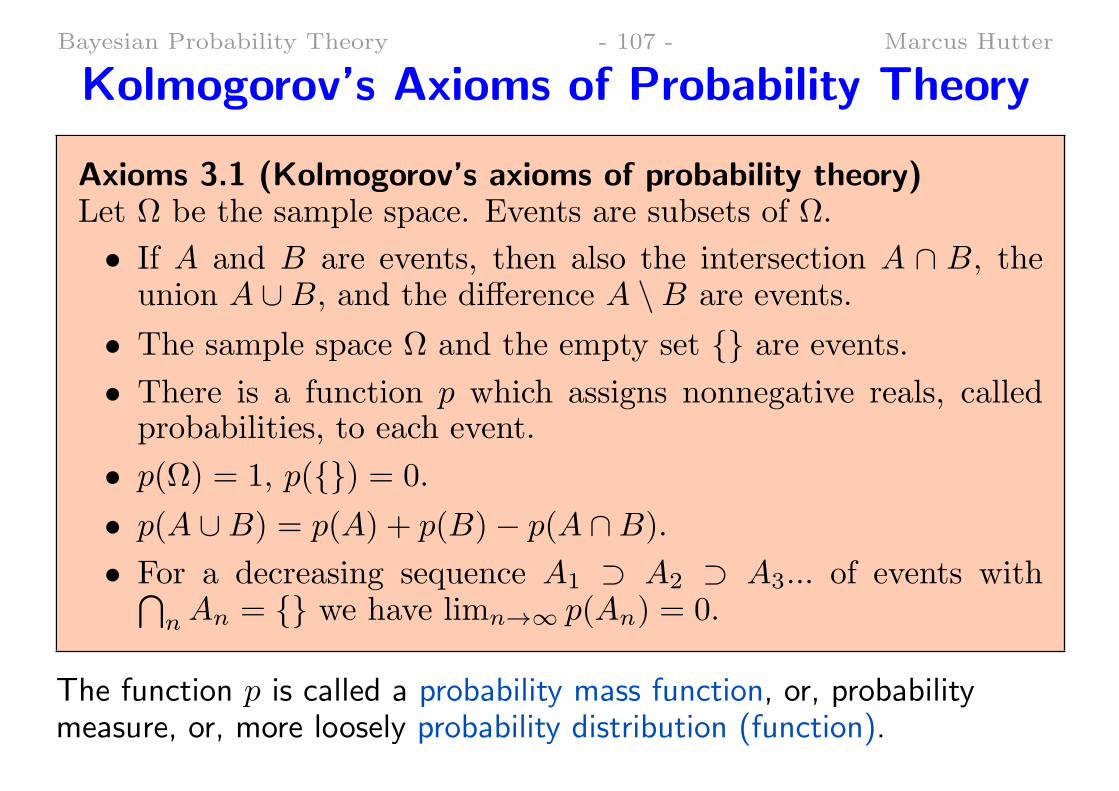
Kolmogorov’s Axioms of Probability Theory
Axioms 3.1 (Kolmogorov’s axioms of probability theory)Let Ω be the sample space. Events are subsets of Ω.
• If A and B are events, then also the intersection A ∩ B, theunion A ∪B, and the difference A \B are events.
• The sample space Ω and the empty set are events.
• There is a function p which assigns nonnegative reals, calledprobabilities, to each event.
• p(Ω) = 1, p() = 0.
• p(A ∪B) = p(A) + p(B)− p(A ∩B).
• For a decreasing sequence A1 ⊃ A2 ⊃ A3... of events with∩nAn = we have limn→∞ p(An) = 0.
The function p is called a probability mass function, or, probabilitymeasure, or, more loosely probability distribution (function).
Bayesian Probability Theory - 108 - Marcus Hutter
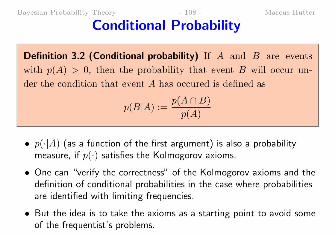
Conditional Probability
Definition 3.2 (Conditional probability) If A and B are events
with p(A) > 0, then the probability that event B will occur un-
der the condition that event A has occured is defined as
p(B|A) := p(A ∩B)
p(A)
• p(·|A) (as a function of the first argument) is also a probabilitymeasure, if p(·) satisfies the Kolmogorov axioms.
• One can “verify the correctness” of the Kolmogorov axioms and thedefinition of conditional probabilities in the case where probabilitiesare identified with limiting frequencies.
• But the idea is to take the axioms as a starting point to avoid someof the frequentist’s problems.
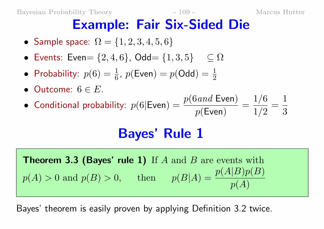
Bayesian Probability Theory - 109 - Marcus Hutter
Example: Fair Six-Sided Die• Sample space: Ω = 1, 2, 3, 4, 5, 6• Events: Even= 2, 4, 6, Odd= 1, 3, 5 ⊆ Ω
• Probability: p(6) = 16 , p(Even) = p(Odd) = 1
2
• Outcome: 6 ∈ E.
• Conditional probability: p(6|Even) = p(6and Even)
p(Even)=
1/6
1/2=
1
3
Bayes’ Rule 1
Theorem 3.3 (Bayes’ rule 1) If A and B are events with
p(A) > 0 and p(B) > 0, then p(B|A) = p(A|B)p(B)
p(A)
Bayes’ theorem is easily proven by applying Definition 3.2 twice.
Bayesian Probability Theory - 110 - Marcus Hutter
3.3 Subjective Interpretation:
Degrees of Belief: Contents
• Subjective Interpretation: Degrees of Belief
• Cox’s Axioms for Beliefs
• Cox’s Theorem
• Bayes’ Famous Rule
Bayesian Probability Theory - 111 - Marcus Hutter
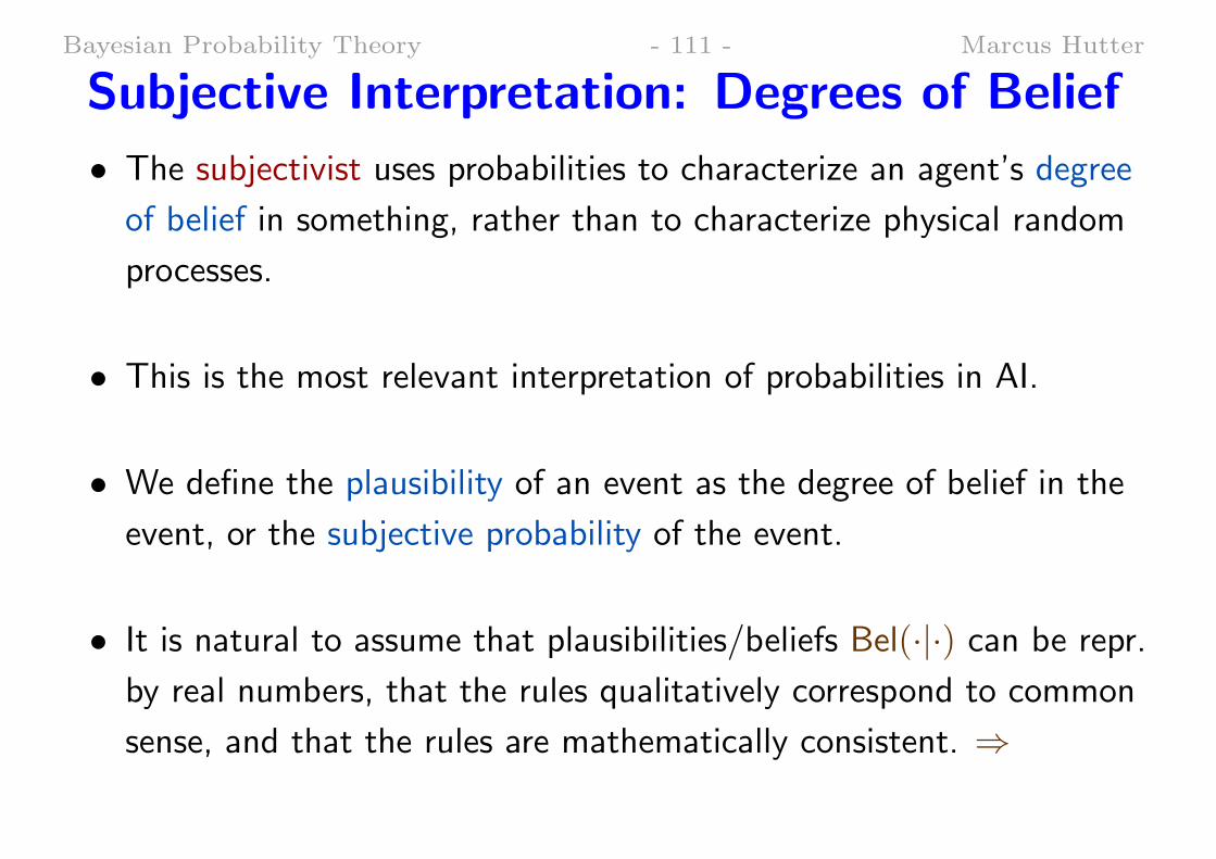
Subjective Interpretation: Degrees of Belief
• The subjectivist uses probabilities to characterize an agent’s degree
of belief in something, rather than to characterize physical random
processes.
• This is the most relevant interpretation of probabilities in AI.
• We define the plausibility of an event as the degree of belief in the
event, or the subjective probability of the event.
• It is natural to assume that plausibilities/beliefs Bel(·|·) can be repr.
by real numbers, that the rules qualitatively correspond to common
sense, and that the rules are mathematically consistent. ⇒
Bayesian Probability Theory - 112 - Marcus Hutter
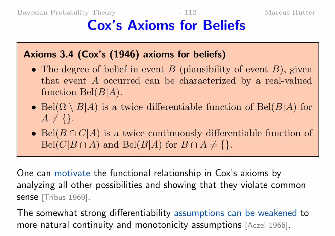
Cox’s Axioms for Beliefs
Axioms 3.4 (Cox’s (1946) axioms for beliefs)
• The degree of belief in event B (plausibility of event B), giventhat event A occurred can be characterized by a real-valuedfunction Bel(B|A).
• Bel(Ω \ B|A) is a twice differentiable function of Bel(B|A) forA = .
• Bel(B ∩ C|A) is a twice continuously differentiable function ofBel(C|B ∩A) and Bel(B|A) for B ∩A = .
One can motivate the functional relationship in Cox’s axioms byanalyzing all other possibilities and showing that they violate commonsense [Tribus 1969].
The somewhat strong differentiability assumptions can be weakened tomore natural continuity and monotonicity assumptions [Aczel 1966].
Bayesian Probability Theory - 113 - Marcus Hutter
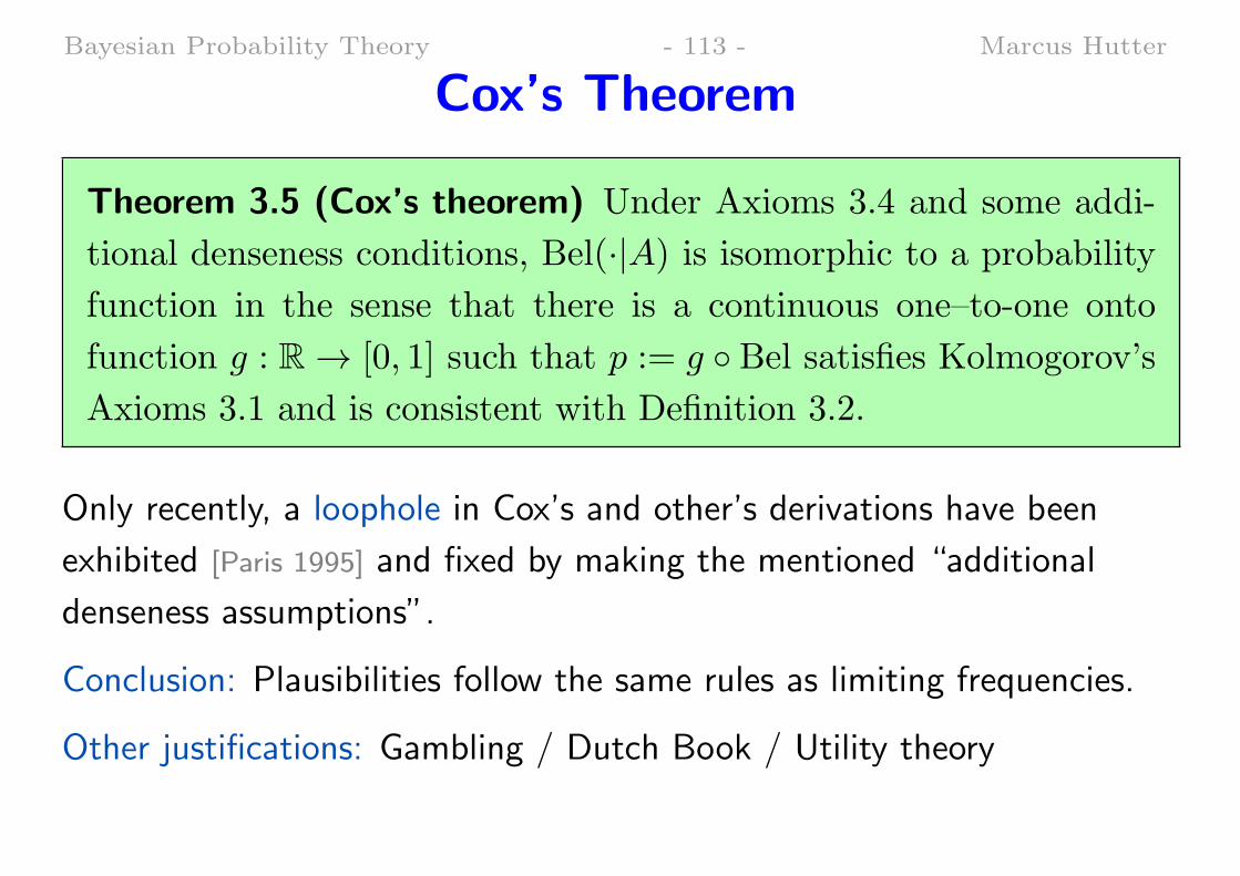
Cox’s Theorem
Theorem 3.5 (Cox’s theorem) Under Axioms 3.4 and some addi-
tional denseness conditions, Bel(·|A) is isomorphic to a probability
function in the sense that there is a continuous one–to-one onto
function g : R → [0, 1] such that p := g Bel satisfies Kolmogorov’s
Axioms 3.1 and is consistent with Definition 3.2.
Only recently, a loophole in Cox’s and other’s derivations have been
exhibited [Paris 1995] and fixed by making the mentioned “additional
denseness assumptions”.
Conclusion: Plausibilities follow the same rules as limiting frequencies.
Other justifications: Gambling / Dutch Book / Utility theory
Bayesian Probability Theory - 114 - Marcus Hutter
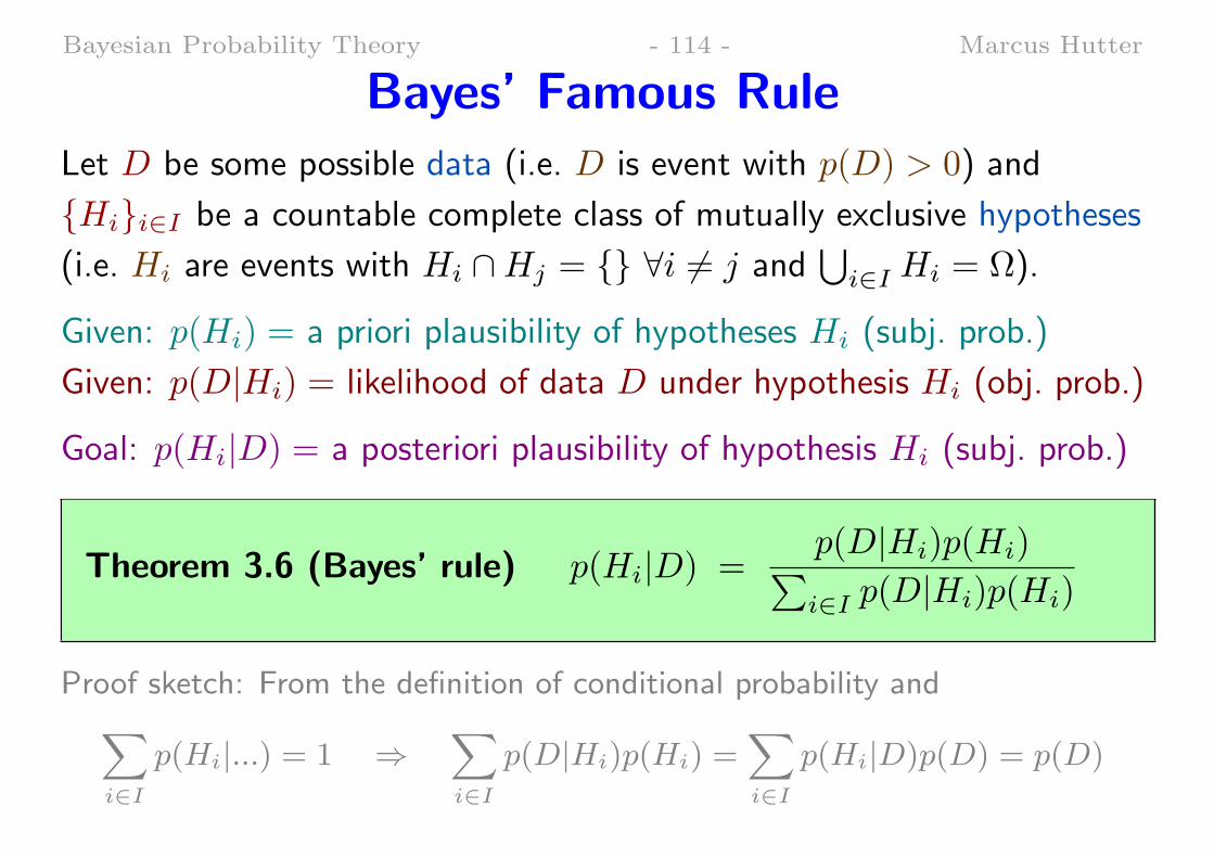
Bayes’ Famous Rule
Let D be some possible data (i.e. D is event with p(D) > 0) and
Hii∈I be a countable complete class of mutually exclusive hypotheses
(i.e. Hi are events with Hi ∩Hj = ∀i = j and∪
i∈I Hi = Ω).
Given: p(Hi) = a priori plausibility of hypotheses Hi (subj. prob.)
Given: p(D|Hi) = likelihood of data D under hypothesis Hi (obj. prob.)
Goal: p(Hi|D) = a posteriori plausibility of hypothesis Hi (subj. prob.)
Theorem 3.6 (Bayes’ rule) p(Hi|D) =p(D|Hi)p(Hi)∑i∈I p(D|Hi)p(Hi)
Proof sketch: From the definition of conditional probability and∑i∈I
p(Hi|...) = 1 ⇒∑i∈I
p(D|Hi)p(Hi) =∑i∈I
p(Hi|D)p(D) = p(D)
Bayesian Probability Theory - 115 - Marcus Hutter
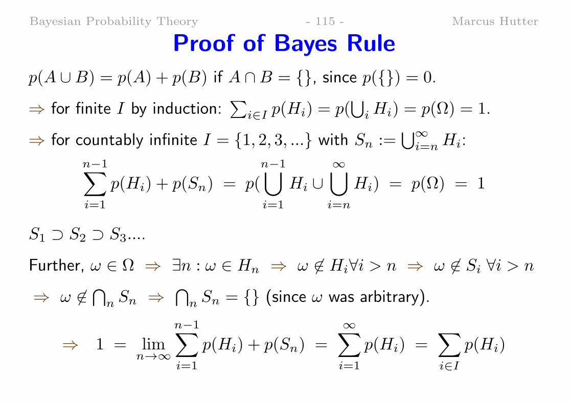
Proof of Bayes Rule
p(A ∪B) = p(A) + p(B) if A ∩B = , since p() = 0.
⇒ for finite I by induction:∑
i∈I p(Hi) = p(∪
iHi) = p(Ω) = 1.
⇒ for countably infinite I = 1, 2, 3, ... with Sn :=∪∞
i=nHi:
n−1∑i=1
p(Hi) + p(Sn) = p(n−1∪i=1
Hi ∪∞∪i=n
Hi) = p(Ω) = 1
S1 ⊃ S2 ⊃ S3....
Further, ω ∈ Ω ⇒ ∃n : ω ∈ Hn ⇒ ω ∈ Hi∀i > n ⇒ ω ∈ Si ∀i > n
⇒ ω ∈∩
n Sn ⇒∩
n Sn = (since ω was arbitrary).
⇒ 1 = limn→∞
n−1∑i=1
p(Hi) + p(Sn) =∞∑i=1
p(Hi) =∑i∈I
p(Hi)
Bayesian Probability Theory - 116 - Marcus Hutter
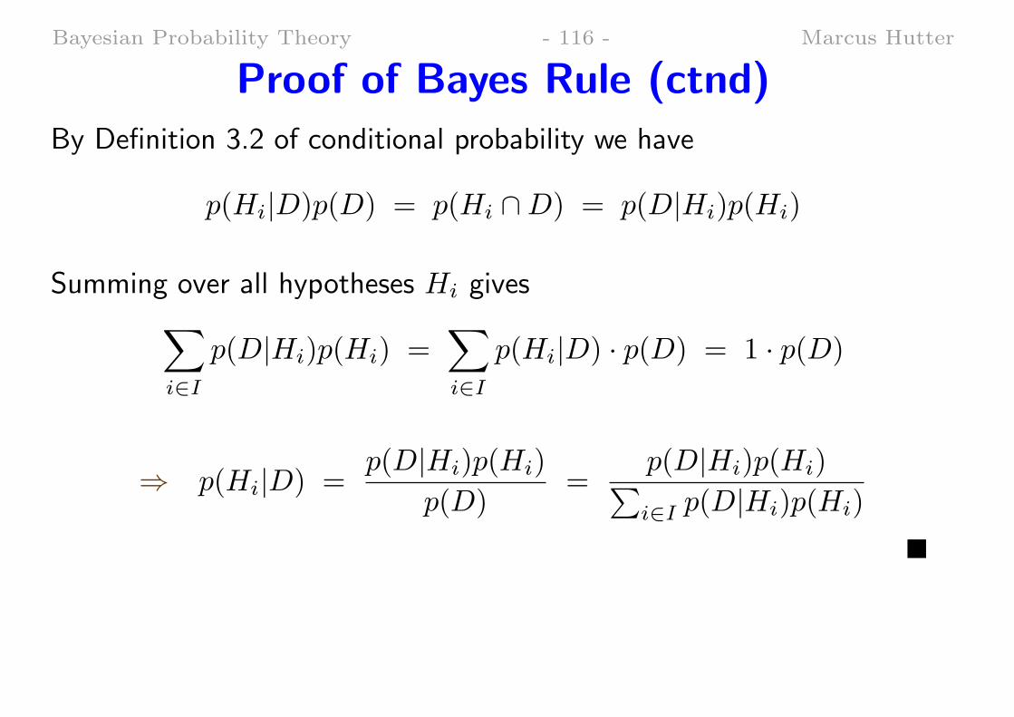
Proof of Bayes Rule (ctnd)
By Definition 3.2 of conditional probability we have
p(Hi|D)p(D) = p(Hi ∩D) = p(D|Hi)p(Hi)
Summing over all hypotheses Hi gives∑i∈I
p(D|Hi)p(Hi) =∑i∈I
p(Hi|D) · p(D) = 1 · p(D)
⇒ p(Hi|D) =p(D|Hi)p(Hi)
p(D)=
p(D|Hi)p(Hi)∑i∈I p(D|Hi)p(Hi)
Bayesian Probability Theory - 117 - Marcus Hutter
3.4 Determining Priors: Contents
• How to Choose the Prior?
• Indifference or Symmetry Principle
• Example: Bayes’ and Laplace’s Rule
• The Maximum Entropy Principle ...
• Occam’s Razor — The Simplicity Principle
Bayesian Probability Theory - 118 - Marcus Hutter
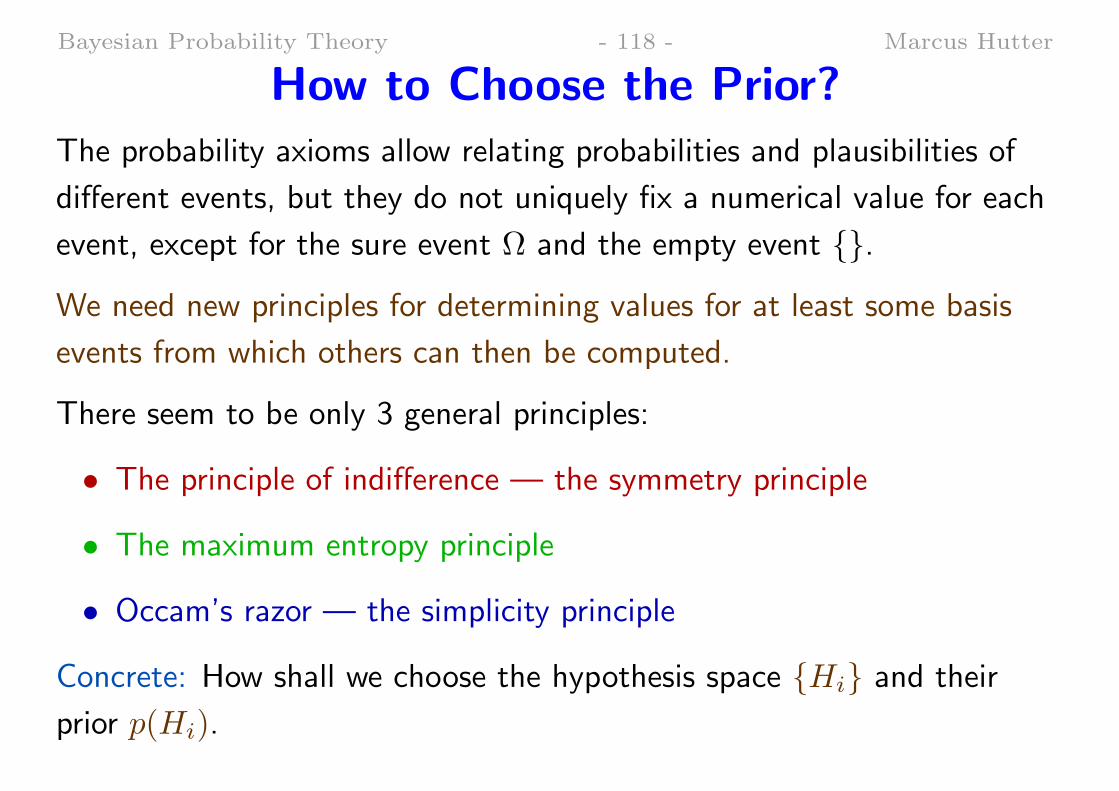
How to Choose the Prior?
The probability axioms allow relating probabilities and plausibilities of
different events, but they do not uniquely fix a numerical value for each
event, except for the sure event Ω and the empty event .
We need new principles for determining values for at least some basis
events from which others can then be computed.
There seem to be only 3 general principles:
• The principle of indifference — the symmetry principle
• The maximum entropy principle
• Occam’s razor — the simplicity principle
Concrete: How shall we choose the hypothesis space Hi and their
prior p(Hi).
Bayesian Probability Theory - 119 - Marcus Hutter
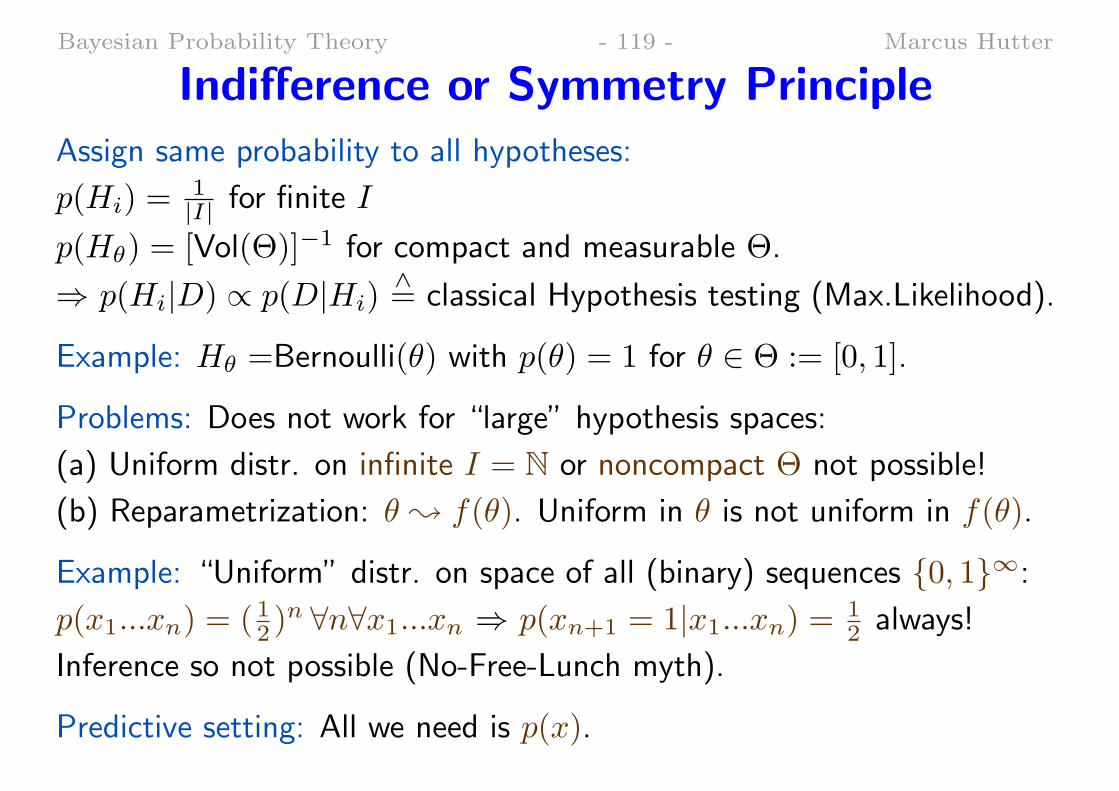
Indifference or Symmetry Principle
Assign same probability to all hypotheses:
p(Hi) =1|I| for finite I
p(Hθ) = [Vol(Θ)]−1 for compact and measurable Θ.
⇒ p(Hi|D) ∝ p(D|Hi)∧= classical Hypothesis testing (Max.Likelihood).
Example: Hθ =Bernoulli(θ) with p(θ) = 1 for θ ∈ Θ := [0, 1].
Problems: Does not work for “large” hypothesis spaces:
(a) Uniform distr. on infinite I = N or noncompact Θ not possible!
(b) Reparametrization: θ ; f(θ). Uniform in θ is not uniform in f(θ).
Example: “Uniform” distr. on space of all (binary) sequences 0, 1∞:
p(x1...xn) = ( 12 )n ∀n∀x1...xn ⇒ p(xn+1 = 1|x1...xn) = 1
2 always!
Inference so not possible (No-Free-Lunch myth).
Predictive setting: All we need is p(x).
Bayesian Probability Theory - 120 - Marcus Hutter
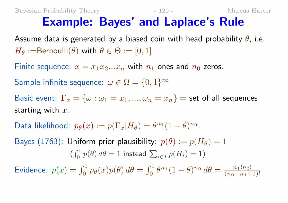
Example: Bayes’ and Laplace’s Rule
Assume data is generated by a biased coin with head probability θ, i.e.
Hθ :=Bernoulli(θ) with θ ∈ Θ := [0, 1].
Finite sequence: x = x1x2...xn with n1 ones and n0 zeros.
Sample infinite sequence: ω ∈ Ω = 0, 1∞
Basic event: Γx = ω : ω1 = x1, ..., ωn = xn = set of all sequences
starting with x.
Data likelihood: pθ(x) := p(Γx|Hθ) = θn1(1− θ)n0 .
Bayes (1763): Uniform prior plausibility: p(θ) := p(Hθ) = 1
(∫ 1
0p(θ) dθ = 1 instead
∑i∈I p(Hi) = 1)
Evidence: p(x) =∫ 1
0pθ(x)p(θ) dθ =
∫ 1
0θn1(1− θ)n0 dθ = n1!n0!
(n0+n1+1)!
Bayesian Probability Theory - 121 - Marcus Hutter
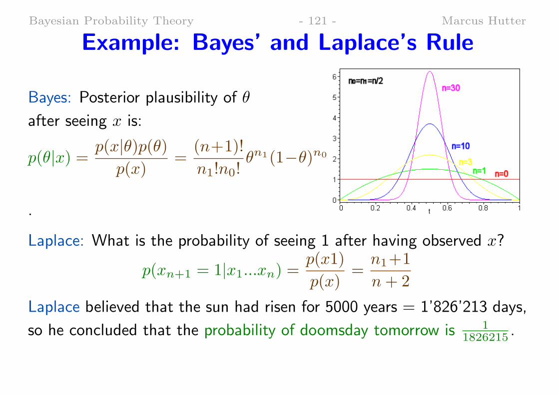
Example: Bayes’ and Laplace’s Rule
Bayes: Posterior plausibility of θ
after seeing x is:
p(θ|x) = p(x|θ)p(θ)p(x)
=(n+1)!
n1!n0!θn1(1−θ)n0
.
Laplace: What is the probability of seeing 1 after having observed x?
p(xn+1 = 1|x1...xn) =p(x1)
p(x)=n1+1
n+ 2
Laplace believed that the sun had risen for 5000 years = 1’826’213 days,
so he concluded that the probability of doomsday tomorrow is 11826215 .
Bayesian Probability Theory - 122 - Marcus Hutter
The Maximum Entropy Principle ...
... is based on the foundations of statistical physics.
... chooses among a class of distributions the one which has maximal
entropy.
The class is usually characterized by constraining the class of all
distributions.
... generalizes the symmetry principle.
... reduces to the symmetry principle in the special case of no
constraint.
... has same limitations as the symmetry principle.
Bayesian Probability Theory - 123 - Marcus Hutter
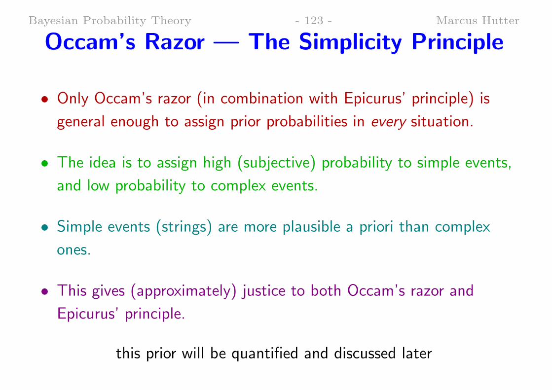
Occam’s Razor — The Simplicity Principle
• Only Occam’s razor (in combination with Epicurus’ principle) is
general enough to assign prior probabilities in every situation.
• The idea is to assign high (subjective) probability to simple events,
and low probability to complex events.
• Simple events (strings) are more plausible a priori than complex
ones.
• This gives (approximately) justice to both Occam’s razor and
Epicurus’ principle.
this prior will be quantified and discussed later
Bayesian Probability Theory - 124 - Marcus Hutter
3.5 Discussion: Contents
• Probability Jargon
• Applications
• Outlook
• Summary
• Exercises
• Literature
Bayesian Probability Theory - 125 - Marcus Hutter
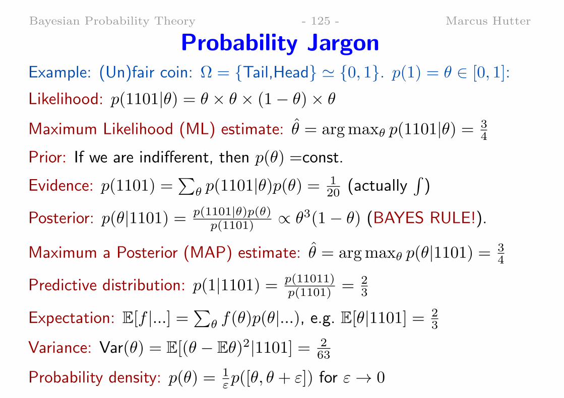
Probability JargonExample: (Un)fair coin: Ω = Tail,Head ≃ 0, 1. p(1) = θ ∈ [0, 1]:
Likelihood: p(1101|θ) = θ × θ × (1− θ)× θ
Maximum Likelihood (ML) estimate: θ = argmaxθ p(1101|θ) = 34
Prior: If we are indifferent, then p(θ) =const.
Evidence: p(1101) =∑
θ p(1101|θ)p(θ) =120 (actually
∫)
Posterior: p(θ|1101) = p(1101|θ)p(θ)p(1101) ∝ θ3(1− θ) (BAYES RULE!).
Maximum a Posterior (MAP) estimate: θ = argmaxθ p(θ|1101) = 34
Predictive distribution: p(1|1101) = p(11011)p(1101) = 2
3
Expectation: E[f |...] =∑
θ f(θ)p(θ|...), e.g. E[θ|1101] =23
Variance: Var(θ) = E[(θ − Eθ)2|1101] = 263
Probability density: p(θ) = 1εp([θ, θ + ε]) for ε→ 0
Bayesian Probability Theory - 126 - Marcus Hutter
Applications
• Bayesian dependency networks
• (Naive) Bayes classification
• Bayesian regression
• Model parameter estimation
• Probabilistic reasoning systems
• Pattern recognition
• ...
Bayesian Probability Theory - 127 - Marcus Hutter
Outlook
• Likelihood functions from the exponential family
(Gauss, Multinomial, Poisson, Dirichlet)
• Conjugate priors
• Approximations: Gaussian, Laplace, Gradient Descent, ...
• Monte Carlo simulations: Gibbs sampling, Metropolis-Hastings,
• Bayesian model comparison
• Consistency of Bayesian estimators
Bayesian Probability Theory - 128 - Marcus Hutter
Summary
• The aim of probability theory is to describe uncertainty.
• Frequency interpretation of probabilities is simple,
but is circular and limited to i.i.d.
• Distinguish between subjective and objective probabilities.
• Both kinds of probabilities satisfy Kolmogorov’s axioms.
• Use Bayes rule for getting posterior from prior probabilities.
• But where do the priors come from?
• Occam’s razor: Choose a simplicity biased prior.
• Still: What do objective probabilities really mean?
Bayesian Probability Theory - 129 - Marcus Hutter
Exercise 1 [C25] Envelope Paradox
• I offer you two closed envelopes, one of them contains twice the
amount of money than the other. You are allowed to pick one and
open it. Now you have two options. Keep the money or decide for
the other envelope (which could double or half your gain).
• Symmetry argument: It doesn’t matter whether you switch, the
expected gain is the same.
• Refutation: With probability p = 1/2, the other envelope contains
twice/half the amount, i.e. if you switch your expected gain
increases by a factor 1.25=1/2*2+1/2*1/2.
• Present a Bayesian solution.
Bayesian Probability Theory - 130 - Marcus Hutter
Exercise 2 [C15-45] Confirmation Paradox(i) R→ B is confirmed by an R-instance with property B
(ii) ¬B → ¬R is confirmed by a ¬B-instance with property ¬R.(iii) Since R→ B and ¬B → ¬R are logically equivalent,R→ B is also confirmed by a ¬B-instance with property ¬R.
Example: Hypothesis (o): All ravens are black (R=Raven, B=Black).
(i) observing a Black Raven confirms Hypothesis (o).
(iii) observing a White Sock also confirms that all Ravens are Black,since a White Sock is a non-Raven which is non-Black.
This conclusion sounds absurd.
Present a Bayesian solution.
Bayesian Probability Theory - 131 - Marcus Hutter
More Exercises
3. [C15] Conditional probabilities: Show that p(·|A) (as a function of
the first argument) also satisfies the Kolmogorov axioms, if p(·)does.
4. [C20] Prove Bayes rule (Theorem 3.6).
5. [C05] Assume the prevalence of a certain disease in the general
population is 1%. Assume some test on a diseased/healthy person
is positive/negative with 99% probability. If the test is positive,
what is the chance of having the disease?
6. [C20] Compute∫ 1
0θn(1− θ)m dθ (without looking it up)
Bayesian Probability Theory - 132 - Marcus Hutter
Literature (from easy to hard)
[Jay03] E. T. Jaynes. Probability Theory: The Logic of Science. CambridgeUniversity Press, Cambridge, MA, 2003.
[Bis06] C. M. Bishop. Pattern Recognition and Machine Learning. Springer,2006.
[Pre02] S. J. Press. Subjective and Objective Bayesian Statistics: Principles,Models, and Applications. Wiley, 2nd edition, 2002.
[GCSR95] A. Gelman, J. B. Carlin, H. S. Stern, and D. B. Rubin.Bayesian Data Analysis. Chapman & Hall / CRC, 1995.
[Fel68] W. Feller. An Introduction to Probability Theory and itsApplications. Wiley, New York, 3rd edition, 1968.
[Sze86] G. J. Szekely. Paradoxes in Probability Theory and MathematicalStatistics. Reidel, Dordrecht, 1986.
![Studies on the Carburizing Process of AISI 8620 Steel · technology of the AISI 8620 steel grade (MIM samples) [3], and the other category consists of pieces made by conventional](https://img.pdfslide.us/doc/110x75/5ec1134807a24453ef302346/studies-on-the-carburizing-process-of-aisi-8620-technology-of-the-aisi-8620-steel.jpg)