Embed Size (px)
Citation preview

DI
SC
US
SI
ON
P
AP
ER
S
ER
IE
S
Forschungsinstitut zur Zukunft der ArbeitInstitute for the Study of Labor
Commuting, Wages and Bargaining Power
IZA DP No. 4510
October 2009
Peter RupertElena StancanelliEtienne Wasmer

Commuting, Wages and
Bargaining Power
Peter Rupert University of California, Santa Barbara
Elena Stancanelli
CNRS, THEMA, University Cergy
Etienne Wasmer Sciences-Po Paris, OFCE,
CEPR and IZA
Discussion Paper No. 4510 October 2009
IZA
P.O. Box 7240 53072 Bonn
Germany
Phone: +49-228-3894-0 Fax: +49-228-3894-180
E-mail: [email protected]
Any opinions expressed here are those of the author(s) and not those of IZA. Research published in this series may include views on policy, but the institute itself takes no institutional policy positions. The Institute for the Study of Labor (IZA) in Bonn is a local and virtual international research center and a place of communication between science, politics and business. IZA is an independent nonprofit organization supported by Deutsche Post Foundation. The center is associated with the University of Bonn and offers a stimulating research environment through its international network, workshops and conferences, data service, project support, research visits and doctoral program. IZA engages in (i) original and internationally competitive research in all fields of labor economics, (ii) development of policy concepts, and (iii) dissemination of research results and concepts to the interested public. IZA Discussion Papers often represent preliminary work and are circulated to encourage discussion. Citation of such a paper should account for its provisional character. A revised version may be available directly from the author.

IZA Discussion Paper No. 4510 October 2009
ABSTRACT
Commuting, Wages and Bargaining Power* A search model of the labor market is augmented to include commuting time to work. The theory posits that wages are positively related to commute distance, by a factor itself depending negatively on the bargaining power of workers. Since not all combinations of distance and wages are accepted, there is non-random selection of accepted job offers. We build on these ingredients to explore in the data the relationship between wages and commute time. We find that neglecting to account for this selection will bias downward the wage impact of commuting, and marginally affect the coefficients on education, age and gender. The correlation between the residuals of the selectivity equation and the distance equation is -0.70, showing the large impact of commute time on job acceptance decisions. We also use the theory to calculate the bargaining power of workers which largely varies depending on demographic groups: it appears to be much larger for men than that for women and that the bargaining power of women with young children is essentially zero. JEL Classification: J3, J6, R2 Keywords: commuting, search model, simultaneous equations Corresponding author: Etienne Wasmer Sciences Po - OFCE 69 Quai d'Orsay 75340 Paris Cedex 07 France E-mail: [email protected]
* We thank the editor, anonymous referees, Ping Wang and participants at the University of Wisconsin/Atlanta Fed Conference on Housing for comments and suggestions and Gong Cheng for excellent research assistance.

1 Introduction
The job search model, based on the work of McCall-Mortensen-Pissarides, has become the workhorse
to describe the outcome of decisions by workers and firms in terms of the aggregate labor market.
Such models can be characterized by search and recruiting frictions and by the necessity of reallo-
cating workers to jobs due to separations. As such, workers are willing to accept any job that pays
a wage higher than their reservation wage. However, the wage is only one attribute of the decision
to accept a job. We argue in this paper that commuting time or distance plays an important role in
the decision to accept or reject a job.
Search theory has long recognized the role of geographical distance and commuting costs.
Stigler (1961) argued that price ignorance was in large part due to geographical dispersion. Lucas
and Prescott (1974) have a spatial dispersion of labor markets and there is a cost (a period of unem-
ployment) of moving between islands. Diamond (1981, 1982) introduces costs of making draws
to get a new offer which is, implicitly or explicitly, a moving cost, i.e., the cost of finding a trading
partner. Gaumont, Schindler, and Wright (2006) show that the introduction of commuting costs can
resolve the Diamond Paradox, leading to a dispersion of wages. Wasmer and Zenou (2006) show
that labor and housing markets interact when distance affects search efficiency, in particular that
spatial segregation is more likely to occur in downturns. Manning (2003) uses the dependence of
separations due to commute distance as evidence of monopsony power of employers, as wages do
not fully reflect the cost of commuting. Van Ommeren, Van den Berg, and Gorter (2000) estimate
a structural search model with on-the-job mobility and identify the marginal cost of commuting
time found to be approximately half of the hourly wage per hour of commute. Van den Berg and
Gorter (1997) find that among demographic groups, females with children face a higher disutility
of commuting, while being in a region with higher unemployment reduces this disutility parameter.
Gautier and Zenou (2008) show that the cost and difficulty of black workers to buy a car leads to
an amplification of spatial mismatch, that is, the difficulty of black workers to access jobs located
in suburbs. Fu and Ross (2009) using average workplace commute times to test whether location
based productivity differences are compensated away by longer commutes, estimate that the total
2

-time and monetary- cost of commuting, as capitalized into wages, is about double the wage rate
in the United States.
Our model also implies an estimate of the bargaining power of workers. The findings show
that overall bargaining power of workers is 0.42 on average with large heterogeneity: 0.73 for
men, 0.15 for women and almost zero for women with young children.
Despite these papers, there are very few search models in macroeconomic theory where com-
mute costs play a central role. Rupert and Wasmer (2008) build the dual of a search and matching
model, where random wage offers are replaced by random “commute-distance offers” and where
workers can relocate at some cost to better locations. They argue that housing frictions differ
across countries, and that cross-country differences in housing frictions can (i) explain large dif-
ferences in geographical mobility between Europe and the US, and (ii) explain a significant part of
the difference in unemployment rates.
In this paper, we document further the role of commute distance. First, we present some
evidence showing the importance of commuting time. Second, we develop a simple theory of job
offers in which jobs have two components: A productivity component and a commute distance
component. We show reservation strategies and the role of distance in determining wages. Third,
we document the correlation between wages and commute distance using a very detailed French
time-use survey. Finally, we use the theory to measure the bargaining power of workers.
In the model, workers have a reservation strategy where wages and commute distance matter:
Accepted offers must generate a positive link between commute distance and wages. Productivity
itself may depend on commute distance. That is, workers may be more tired from long commutes,
thus generating a negative link between productivity and commute distance. Conversely, job offers
located in more remote locations may be of higher productivity if workers’ skills are heteroge-
neous and match productivity is idiosyncratic, as workers might target their job search to the most
profitable areas when commutes are long.
We find that neglecting the commute distance equation in the estimates of wage equations
seriously biases downward the wage impact of commute, and marginally affects the coefficient on
3

education, age and gender. The correlation between the residuals of the selectivity equation and the
distance equation is -0.70, showing the large impact of commute time on job acceptance decisions.
2 Commuting
In this paper, we argue that commuting distance plays an important role when deciding whether to
accept a job. Table 1 reports data from a European-wide panel (the ECHP panel 1994-2001) for
a sample of currently unemployed job seekers.1 These individuals received a job offer during the
past 4 weeks and rejected it.
Table 1: Reasons for Rejecting Offers
% % excl.last 3
% excl.last 3 & hrs
% comparedto wage rate
1. rate of pay 12.1 21.8 24.7 59.72. temporary/insecure job 6.65 12.0 13.6 -3. type of work 12.9 23.3 26.4 -4. number of working hours 6.05 11.0 - -5. working time (day time, night time, shifts...) 6.42 11.6 12.4 -6. working conditions / environment 3.06 5.54 6.27 -7. distance to job / commuting 8.14 14.7 16.7 40.38. could not start the job at required time 4.82 - - -9. other reasons for not accepting 20.99 - - -10. not yet decided 18.93 - - -Sum 100 100 100 100
Column 1 of Table 1 shows that roughly 40% of individuals interviewed had not yet decided to
accept the offer or were not available to take the offer for other reasons (reasons 8 and 9). Column
2 excludes those individuals, thus revealing that 14.7% of job offers were turned down due to
commute distance; 16.7% if one further excludes the jobs rejected due to the offered number of
hours. Finally, the last column indicates that the weight given to commute distance is roughly a
third lower than the importance of the wage rate when the job acceptance decision has to be made.1Those having no job and are looking for one or currently working less than 15 hours and looking for an additional
one or a different one.
4

3 Model
3.1 Standard search setup
In the standard search model a la McCall, workers decide whether to accept a job offer based
on the wage they get and the distribution of the known potential wage offers. The decision to
work is based on a comparison of the value of being in an employment relationship to the value
of remaining unemployed. In a continuous time setup, the canonical job-search model can be
summarized as:
rU = b+λ
∫Max(0,E(w′)−U)dF(w) (1)
rE(w) = w−C(h)+δ (U−E), (2)
where r is the rate of interest, b is the value of unemployment benefits, λ is the arrival rate of job
offers, δ is an exogenous job destruction rate, F is the c.d.f. of wage offers, C(h) is the cost of
working h hours (assumed to be fixed due to some indivisibility) and E and U are the present-
discounted values of being employed and unemployed, respectively.
Noting that equation Eq. (1) is increasing in w with constant slope 1/(r +δ ) leads to
E(w)−U =w−wR
r +δ. (3)
The positive slope implies that there is a well-defined reservation rule wR, which can be defined
implicitly by U = E(wR), that is
wR = b+C(h)+λ
r +δ
∫ +∞
wR(w−wR)dF(w). (4)
Knowledge of the reservation wage, wR, has implications for the rate of unemployment, given by:
u =δ
δ +λ [1−F(wR)].
5
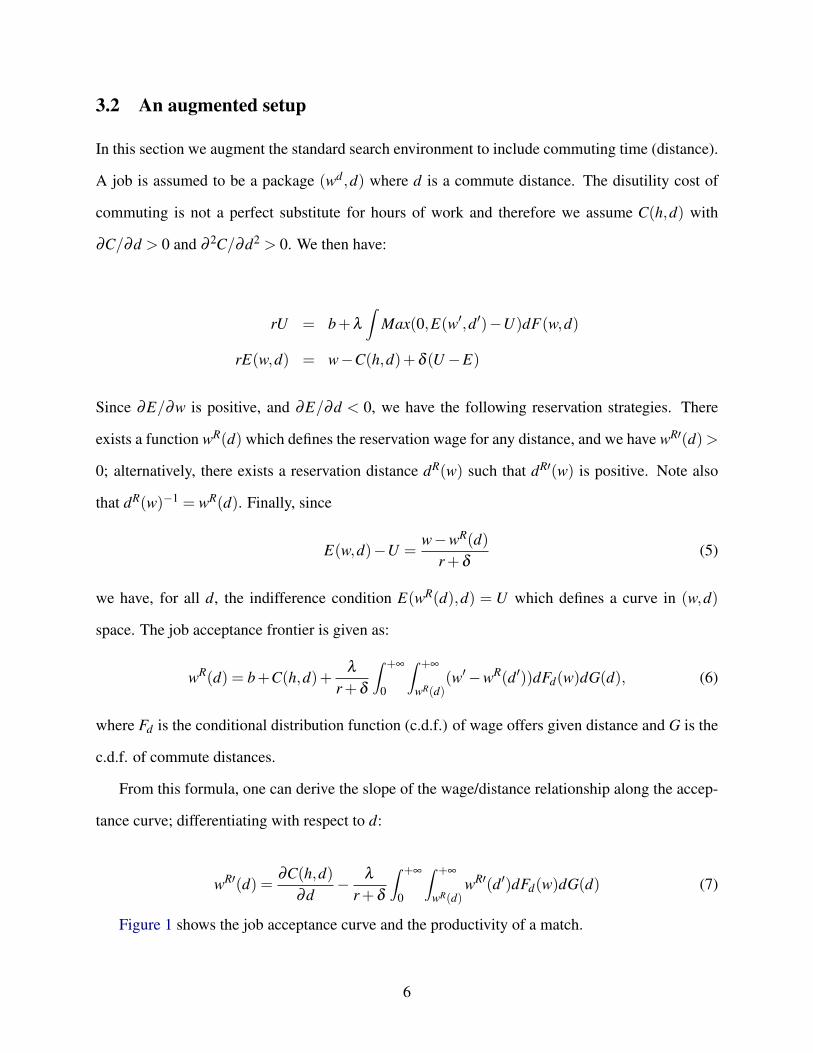
3.2 An augmented setup
In this section we augment the standard search environment to include commuting time (distance).
A job is assumed to be a package (wd,d) where d is a commute distance. The disutility cost of
commuting is not a perfect substitute for hours of work and therefore we assume C(h,d) with
∂C/∂d > 0 and ∂ 2C/∂d2 > 0. We then have:
rU = b+λ
∫Max(0,E(w′,d′)−U)dF(w,d)
rE(w,d) = w−C(h,d)+δ (U−E)
Since ∂E/∂w is positive, and ∂E/∂d < 0, we have the following reservation strategies. There
exists a function wR(d) which defines the reservation wage for any distance, and we have wR′(d) >
0; alternatively, there exists a reservation distance dR(w) such that dR′(w) is positive. Note also
that dR(w)−1 = wR(d). Finally, since
E(w,d)−U =w−wR(d)
r +δ(5)
we have, for all d, the indifference condition E(wR(d),d) = U which defines a curve in (w,d)
space. The job acceptance frontier is given as:
wR(d) = b+C(h,d)+λ
r +δ
∫ +∞
0
∫ +∞
wR(d)(w′−wR(d′))dFd(w)dG(d), (6)
where Fd is the conditional distribution function (c.d.f.) of wage offers given distance and G is the
c.d.f. of commute distances.
From this formula, one can derive the slope of the wage/distance relationship along the accep-
tance curve; differentiating with respect to d:
wR′(d) =∂C(h,d)
∂d− λ
r +δ
∫ +∞
0
∫ +∞
wR(d)wR′(d′)dFd(w)dG(d) (7)
Figure 1 shows the job acceptance curve and the productivity of a match.
6

Figure 1: Job Acceptance
Frontier of jobacceptance
w
Commutedistance d
Reservationwage for a jobat home
Accepted joboffers
Rejected job offers
Productivity as a function of distance
In the special case where C is increasing and linear in d, wR′ has a constant slope:
wR′ =∂C(h,d)
∂d1
1− λ
r+δa
where 0 < a < 1 is the average acceptance rate.
3.3 Extension: bargaining and commuting
Extending the framework to deal with bargaining is straightforward. Assume that workers draw a
productivity-distance pair, (y,d), where y is productivity. The surplus of the firm is given by
J(y,d) =y−w(y,d)
r +δ. (8)
The Bellman equations for unemployed and employed workers are as follows:
rU = b+λ
∫Max(0,E(y′,d′)−U)dF(y,d) (9)
rE(y,d) = w(y,d)−C(h,d)+δ (U−E). (10)
7

From Eq. (10) we have
E(y,d)−U =w(y,d)−C(h,d)− rU
r +δ(11)
We also assume, consistent with search-matching theory, that firms and workers bargain over
wages as long as there is positive surplus. The bargaining equation solves
βJ(y,d) = (1−β )(E−U), (12)
leading to
w(y,d) = (1−β )rU +(1−β )C(h,d)+βy. (13)
Partial differentiation of the wage equation implies the following results:
∂w∂y
= β and∂w∂d
= (1−β )∂C∂d
(14)
As in the previous section, there exists a well defined reservation strategy. Noting that
∂E∂y
=β
r +δ(15)
∂J∂y
=1−β
r +δ, (16)
and given the monotonicity of asset values, there exists a reservation productivity yR(d). Given the
constant slopes calculated above, we have that
E(y,d)−U = βy− yR(d)
r +δ(17)
J(y,d) = (1−β )y− yR(d)
r +δ. (18)
Finally, yR(d) can be recovered from the fact that workers are indifferent between working and not
working when productivity is equal to the reservation value, that is:
rE(yR(d),d) = rU, (19)
8

Therefore, rU is given as:
rU = b+λ
∫Max(0,E(y′,d′)−U)dF(y,d) = rE(yR(d),d) = w(yR(d),d)−C(h,d)+δ (U−E),
or, after reorganizing terms:
yR(d) = b+C(h,d)+βλ
r +δ
∫ +∞
0
∫ +∞
yR(d)(y′− yR(d′))dFd(w)dG(d). (20)
which is similar to (6).
Proposition 1. Commute distance affects wages: ∂w∂d = (1−β )∂C
∂d .
The proposition states that workers receive higher compensation for commute costs if their
bargaining power is lower. Note that commute costs appear in the wage equation with weight
(1− β ). This is due to the fact that the commute costs are on the “reservation-wage side”. The
term rU +C(h,d) is the opportunity cost of working. The bargained wage is a weighted average of
opportunity cost and the productivity of the match, y. Therefore, the higher the bargaining power,
the closer the wage to the productivity of the match and the further away from the opportunity cost:
the effect of commute costs vanishes when β goes to 1.
4 Wage equations with commute distance
The central idea of our empirical approach is that we extend the search model to allow for com-
muting time. Because wages and commutes are only observed for those accepting a job we model
them simultaneously with the job acceptance probability. Not accounting for selection will give
biased estimates. Therefore, we will provide a simultaneous equations model of wages, commute
and the employment decision to examine the effect of commuting distance on wages. We also
estimate the reservation strategy of agents.
9
4.1 Conditional Mixed Process Estimates: method
We use a simultaneous equations approach to estimate the observed (accepted) wages, the ob-
served (accepted) commuting time and a selection equation, to control for the fact that wages and
commuting time are observed only for people that are employed, i.e., that received a job offer and
accepted it. Therefore, we estimate a conditional (recursive) mixed process model.2 That is, a
simultaneous equation system where the different equations can have different kinds of dependent
variables. To be more precise, recall that jobs are characterized in terms of the wage they offer
and the implied commuting distance and that the probability of receiving a job offer is λ . There-
fore, the reservation wage will also be a function of commuting distance. In particular, reservation
wages are increasing in commuting distance under sticky housing markets. In this paper we do not
have access to reservation wage information. Therefore, we use data on accepted wages, w, with
the implied commuting distance, d, conditional on employment, to estimate the relation between
commuting distance, wages and the employment probability.3
Formally, the employment probability, θ , can be written as the product of the probabilities of
receiving a job offer and accepting it:
θ = λ [1−F(wR(d))], (21)
where F() is the conditional distribution of wages. Thus, commuting distance enters the struc-
tural probability Eq. (21) because of its effect on the reservation wage, which, in turn, affects the
acceptance probability.
We assume that the wage offer distribution and the distribution of distance offers are a function
of individual and match specific characteristics, lognormal and specified as:
wi = g(di)+β′Xi + γ
′Zi + εi, εi ∼ N(0,σ2ε ) (22)
where Xi is a vector containing individual characteristics and Zi a vector of match characteris-
2See Roodman (2007, 2009) for more details.3Reservation wages are rarely observed in the data, exceptions are, for example, Bloemen and Stancanelli (2001),
that used subjective reservation wages in an extended search model.
10

tics. We test whether the functional form of g should be specified as a quadratic to allow for
non-linearities. The error term εi may represent approximation error, measurement error and ran-
domness in preferences.4
To allow for possible correlation of commuting distance with the error of other equations, an
equation for commuting distance is specified as:
di = µ′qi + vi, vi ∼ N(0,σ2
v ), (23)
where q includes individual characteristics.
Accepted wages, with the implied commuting distance, are only observed for employed in-
dividuals, thus we condition on employment by simultaneoulsy specifying an equation for the
employment probability -which is equivalent to the job acceptance probability. The underlying
equation for employment is:
θ∗i = m′ki + ei ei ∼ N(0,τ2), (24)
where ki are individual characteristics and θi = 1 if θ ∗i > 0; θi = 0, otherwise.
We assume joint normality of the error terms of the employment equation, the equation for
wages and the equation for commuting distance. We define ρew as the correlation coefficient
between the errors of the employment equation ei from Eq. (24) and the errors εi of the wage
equation Eq. (22); ρed as the correlation coefficient between the errors of the employment equation
and the errors of the equation for commuting distance vi from Eq. (23), and ρdw as the correlation
between wages and commuting distance.
Under the assumption of joint normality, the employment probability, conditional on the com-
muting distance and the wage, can be written as:
Φ
(m′kiψe|ε,v
σe|ε,v
)(25)
4Structural job search models do not allow for wealth to affect the individual job acceptance decision. An exceptionis Bloemen and Stancanelli (2001) who concluded that reservation wages increase in net wealth.
11

where Φ(.) is the standard normal distribution function and use has been made of the normality
of the distribution of the errors of the employment equation, conditional on commuting distance
and wages. ψ(ei|εit ,vi) is the conditional mean of the error term of the employment equation
(conditional on the errors of commuting time and wages) ; σe|ε,v is the conditional variance of the
error term of the employment equation (conditional on the errors of commuting time and wages).
For each individual, the likelihood contribution is obtained by multiplying the employment
probability by the joint density of commuting and wages.
4.2 Data description
The data for the analysis are drawn from the 1998-99 French time-use survey (Enquete Emploi
du temps), carried out by the National Statistical Office (INSEE). This is a cross-sectional dataset,
providing us with information on individual employment, wages and commuting time. The survey
covers about 8,000 representative households, and includes over 20,000 individuals of all ages,
from 0 to 103 years. Three questionnaires were collected: a household questionnaire, an individual
questionnaire and the time diary. The diary was collected for all individuals in the household, and
was filled in for one day, chosen by the interviewer, and could be either a weekday or a weekend
day.
The individual questionaire also contains a recall question on usual commuting time. There-
fore, an advantage of this dataset is that we can compare commuting time reported from the recall
question with commuting time from the daily diary. It is well-known that recall information is
bound to be less precise. On the other hand, people are likely to know extremely well how much
time on average they spend commuting every day, so that recall bias is unlikely to be very impor-
tant for commuting information. Instead, the diary information on commuting is more likely to be
affected by random variation in commuting, such as, for example, traffic jams. Besides, the day
the diary is collected could fall on a day when people do not work for part-timers or if the diary is
collected on a weekend day. There is also information on their main place of work, which allows
us to determine if an individual’s main job is in their home, in which case their commuting time is
12

Table 2: Sample Selection Criteria
Criterion applied ObservationsSingle people living on their own or in a couple 13473Employed, unemployed or housewives 9251Age less than 60 years 8665
set to zero.
Another advantage of the survey is that it collects earnings information in addition to contrac-
tual hours of work. Total household income is asked, though in brackets. 5 The data also contains
detailed information on individual educational attainment, age, and sex, which we also use in our
model.
Other variables in the data set allow us to control for factors that might affect mobility, such as
home ownership, duration of occupation of the residence -which we interact with home ownership-
marital status and presence and age of children.
We select a sample of individuals according to the following criteria:
• single people living on their own or people living as a couple, either married or cohabiting;
• employed; unemployed; housewives/househusbands (We dropped only retirees, those in full-time education, military personnel and the disabled).
• aged less than sixty years.
Information on monthly gross earnings in the year of the survey was collected both as a con-
tinuous variable and in intervals for respondents who did not provide continuous earnings infor-
mation. For them, as noted above, we do not compute hourly wages. To construct the hourly wage
rate, we consider only observations providing information on continous wages and usual hours of
work (roughly half of those who reported earnings). Total household income was set equal to the
5We tried two different specifications for wages: monthly earnings and the hourly wage; however, we generallyreport only the specifications with monthly earnings as the results are more or less equivalent since we have selecteda sample of full-time workers.
13

mid point of each interval; and to the threshold level for individuals in the top income interval.
Non-labor income was constructed by subtracting own earnings from the total household income
variable. Therefore, non-labor income includes earnings of the spouse, if any. All earnings and
income information in the survey was collected in French Francs (equal to 1/6.55957 Euros). Thus,
hourly wages are measured in French Francs; but we transform them to Euros, to make the results
more readable.
We have included dummy variables for education, with the omitted category being individuals
with less than elementary schooling. We also use a series of variables to control for occupation
types, sector and size of firm.
We also control for the size of the area where people reside with a series of dummies as follows:
Paris; suburbs (outskirts) of Paris (banlieue, in French); cities over 50,000 inhabitants ; cities of
20,000 to 50,000 inhabitants; small cities of less than 20,000 inhabitants and rural neighborhoods.
Regional dummies are also included.
Home ownership is a dichomotomous variable equal to one for individuals that own their place
of residence. We also have information in the data on duration of occupancy of the place where
people reside, in years. We have constructed two variables by interacting the duration of occupancy
of the residence with the house ownership dummy: Duration of occupancy of the place where
people reside, in years, for people that rent their residence place; duration of occupancy of the
place where people reside, in years, for people that own their residence place. It may be that
people that live longer in a place are less willing to move and this effect is likely to be stronger for
individuals that own their place of residence.
The marital status dummy is equal to one for married people and to zero for cohabiting or
single people. We consider cohabiting couples as such for several reasons. First, they are subject
to the same income taxation scheme as single people, while married people are taxed jointly.
Second, cohabiting women have participation rates very close to those of single women and much
higher than those of married women. We constructed a dummy variable for the presence of young
children aged less than three in the household. This is the interesting threshold to look at as 99% of
14

children aged three and above go to school in France. Maternelle (pre-school) school for children
aged three to five is free of charge and open from early morning to six in the afternoon. The number
of children aged less than eighteen is also entered among the explanatory variables.
As noted above, the diary day was chosen by the interviewer. Activities were recorded every
ten minutes over a 24-hour period. Both main and secondary activities were coded. These latter
are activities carried out simultaneously, such as cooking and watching the children, with the re-
spondent deciding which activity was primary and which secondary. There were approximately
140 main activity categories and 100 secondary activity categories defined by the survey designers.
Interestingly, all commuting time to work was reported as main activity. Commuting time to work
is coded in minutes.
Descriptive statistics for the full sample are provided in Table 3. Over 50% of the sample is
composed of people that own their residence. The average duration of occupancy of their residence
is about ten years, whether people own it or not. This is slightly larger for women than for men.
Women in full-time employment are, on average, slightly less educated than men. On the other
hand, more women than men have completed secondary education. Average years of schooling
of men and women are the same and equal to just over ten years. The average monthly earnings
of women are almost three hundred Euros less than those of men; and the hourly wage is 2 Euros
smaller.
Commuting time is on average about 45 minutes per day, irrespective of gender. The diary
information records shorter commuting time: forty minutes instead of fifty, according to the recall
question; and slightly less for women than for men. About 24% of the respondents in the sample
reported to be tired from commuting at the end of the day.
Table 4 provides the distribution of monthly earnings and commuting time for the recall ques-
tion and the diary. The distribution of commuting time looks quite skewed. The lowest decile of the
distribution of commuting time of full-time workers, spend less than ten minutes travelling to their
workplace and back. The median full-time worker in the sample commutes forty minutes per day,
while people in the third quartile commute one hour; and those in the top decile, over two hours.
15

Table 3: Summary Statistics-Full Sample
Variable Estimation sample Men WomenN =8665 N =4220 N =4645
Mean Std Dev Mean Std Dev Mean Std DevAge 41.14 9.52 41.48 9.26 40.83 9.74Elementary schooling CEP 0.10 0.30 0.08 0.27 0.11 0.32Lower Secondary tech. bepc 0.08 0.27 0.06 0.24 0.09 0.29Lower Secondary cap-bep 0.30 0.46 0.35 0.48 0.26 0.44Upper Secondary tech bactech 0.06 0.23 0.06 0.24 0.05 0.22Upper Secondary bac 0.08 0.27 0.06 0.23 0.09 0.29Short Univ degree bac+2 0.12 0.32 0.11 0.31 0.13 0.34Univ degree >bac+2 0.12 0.32 0.14 0.34 0.10 0.30School years 10.15 4.34 10.30 4.43 10.02 4.44Married 0.68 0.47 0.69 0.46 0.69 0.47Cohabiting 0.17 0.37 0.18 0.38 0.16 0.37No. of children 1.30 1.22 1.30 1.23 1.29 1.21Children, age < 3 0.13 0.34 0.14 0.34 0.13 0.34Ile de France 0.19 0.39 0.19 0.39 0.19 0.39Cities >=20,000 inhabitantsSmall city <20,000 inhabitants 0.17 0.37 0.17 0.37 0.17 0.37Rural neighborhood 0.26 0.44 0.26 0.44 0.25 0.43Paris 0.03 0.17 0.03 0.17 0.03 0.18Outskirts of Paris 0.13 0.33 0.13 0.34 0.13 0.34French nationality 0.94 0.24 0.94 0.24 0.94 0.23Working mainly at home 0.13 0.34 0.12 0.33 0.14 0.35House ownership 0.57 0.49 0.57 0.49 0.57 0.49Dur. occup. residence, years 9.78 9.13 9.48 9.04 10.05 9.20Monthly Salary, Euros 1338.60 746.45 1557.02 806.69 1111.16 598.83Non labor income, monthly, Euros 2070.75 1335.44 2109.36 1359.83 2036.03 1312.32Hourly wage, Euros 9.08 5.61 9.79 5.85 8.32 5.24Contractual weekly hours 35.75 7.76 37.93 5.57 33.12 8.98Commuting time minutes, recall 44.79 45.21 46.44 46.51 42.94 43.63Commuting time minutes, diary 27.22 42.93 34.49 48.07 20.80 36.64Tired fom commuting, yes ==1 0.16 0.37 0.17 0.37 0.16 0.36
16

The lower-educated people tend to commute a little less than the higher-educated. Married women
in full-time employment commute less time at all percentiles of the distribution of commuting time
than the sample worker.
Table 5 shows the mode of transportation of full-time workers in the sample. Over 70% of
people travel to work by car. This proportion is slightly larger for men, 74%, than for women,
72%. Instead, travelling to work by bus is more common for women, over 9%, than for men, 6%.
Interestingly, almost twice as many women than men go to work on foot (9.2% against 5.6%);
while ten times more men than women use their bycicle or the motorbycicle (almost 3% against
0.6%, for either bycicle or motorbycicle). The differences by gender are smaller for the train (over
1% for either gender) and the metro (3% for men and 4% for women).
4.3 Identification
The identification is as follows. Non-labor income (total household income minus own earnings)
affects the employment decision but not the wage or commuting time equation. By construction,
non-labor income includes the partner’s income, if any, as well as financial rents and dividends.
Structural job search models typically ignore capital accumulation, with the notable exception of
Bloemen and Stancanelli (2001). In the empirical literature, it is customary to assume that non-
labor income affects selection into employment rather than wages. If the wage equation is thought
of as a wage offer, there is no reason for non-labor income to affect it. Non-labor income may
well affect reservation wages, but they are not observed. If a higher reservation wage leads the
individual to reject the wage offer, then this effect will be captured by including non-labor income
among the regressors of the employment acceptance probability. The possible interactions are
captured by the correlations across the errors of the wage and employment equations.
Next, we assume that the size of the area of residence affects the transportation landscape
and therefore the distance equation; but not the employment or wage equations. Instead, regional
dummies enter all equations as they are assumed to measure not only job availability – and thus
the probability of employment – but also different wage premia and transport infrastructure.
17

Table 4: Distribution of commuting time for the estimation sample
Percentiles hourly wage commuting recall commuting diaryFull sample, obs. 3693 4311 41781% 2.91 0 05% 4.51 0 010% 4.87 0 025% 5.86 10 050% 7.49 30 2075% 10.42 60 6090% 14.66 105 9095% 19.54 120 12099% 31.08 180 200Up to elementary school, obs. 879 8341% 2.06 0 05% 3.61 0 010% 4.40 0 025% 5.04 10 050% 6.05 30 2075% 7.22 60 6090% 9.52 90 9095% 11.28 120 12099% 20.10 210 200University degree and above, obs. 1150 11191% 4.22 0 05% 5.59 0 010% 6.54 5 025% 8.57 20 050% 11.30 40 2075% 16.24 70 6090% 23.45 120 10095% 28.87 140 12099% 41.50 210 200Married Women, obs. 1286 12471% 2.08 0 05% 4.04 0 010% 4.64 0 025% 5.41 10 1050% 7.04 30 3075% 9.67 60 6090% 13.62 90 9095% 19.02 120 12099% 20.90 180 180Hourly wages are measured in Euros. Commuting time in minutes.Diary commuting is shown for individuals that also provided recallcommuting information and that were employed.
18

Table 5: Mode of Transportation to Work, %
Sample Men WomenOn foot 7.25 5.59 9.22Bycicle 1.81 2.10 1.47Motorbike 1.81 2.82 0.61Car 73.34 74.41 72.06Train 1.64 1.79 1.47Metro 3.92 3.49 4.44Bus 7.81 6.02 9.44Other 2.41 3.78 0.79Sample size 6398 3470 2928
We also use the duration of occupation of the place of residence to identify the commuting
equation and the employment equation. Indeed, individuals that live longer in a given place may
be less willing to move, as the costs of moving are likely higher for them. This can affect both
the job acceptance probability – and therefore the selection into employment – and the distance
travelled to work. In particular, we use two separate variables, one for the duration of occupation of
the place of residence for renters; and the other for houseowners, both measured in years. We also
assume that the number of children and the presence of small children affect accepted commuting
time and employment, but not wages.6 Instead, gender and marital status enter all three equations
in the form of a dummy for being a woman and an interaction variable of being a woman and being
married, to capture differences across all women and married women, in addition to gender effects.
We identify wages using information on the number of years of work experience. Finally, we
enter a quadratic term in linear commuting time in the wage equation. Schooling years affect
selection and wages but do not impact on commuting distance (we tested for their inclusion in the
distance equation but in line with our expectations, the coefficient was not statistically significant).
In order to avoid having to estimate a singular system, we present a wage equation which does
6Here we assume that wages represent the wage offered and that employers do not discriminate against or in favourof individuals with children. Although there exist a bulk of empirical literature on wage penalties for mothers, recentstudies suggest that these penalties may be applied also to childless women, in expectation that they will later havechildren.
19
depend on commute distance, but a commute distance equation which only depends on individual
and firm’s characteristics.
4.4 Findings
The results are given in Table 6. Observed wages increase with commuting time, though at a
decreasing rate. The correlation coefficients of the three equations are statistically significant, with
a large negative value between the residuals of the employment and the distance equation which is
equal to -0.70. This is rather intuitive: when worker receive a high distance offer, they are much
less likely to accept the package (wage, distance) and therefore more likely to reject the offer. This
tends to suggest that ignoring the selection due to commute distance biases the estimates of the
effect of distance on wages (see below).
Women earn less by 11.1% but their marital status does not affect hourly wages. This might
be due to the fact that all women suffer the same wage penalty as if they were married; that is,
employers may anticipate that single women will marry. We find that wages and employment
increase with education years (schooling years, each additional raising wage by 5.86%). Under
this specification, wages and employment increase with age at a decreasing rate; while the reverse
age pattern applies to commuting time -commuting time falls with age at an increasing rate.
Interestingly, both the number of children and the presence of small children negatively affect
the employment selection, as expected -at least for women, but they impact positively on commut-
ing time. This may indicate that people with small children are prepared to commute further away
and are less willing to move closer to their job (or they have less negotiation power).
Finally, the main effect of commute on wages is quite large. We find that the linear coefficient
of hours of commute is almost a third (+0.327), with a quadratic term equal to -4.18%. This means
that an hour of commute is compensated by a 28.5% increase in wages.
In columns 4 to 5, we report the traditional Heckman selection model where we add commute
hours but do not have a commute time equation. In that case, as well as in column 6 where we
report a simple OLS of wages, the effect of commute time on wages is much smaller, between
20

8.4 and 9.0 percent. This suggests that, due to the strong correlation between the residuals of the
commute time equation and the other equations, ignoring the selectivity in commute time bias the
estimate of the Mincerian wage equation quite seriously.
The estimates of the recursive system equations (columns 1-3) have a few differences with tra-
ditional Heckman (col 4-5) and OLS (col 6) in terms of the effects of other variables. For instance,
the effect of education on wages is half of a percentage point lower (5.86% instead of 6.38%), the
effect of age is one percentage point above for the first years (3.38% instead of 2.27%), the wage
discount of women is two percentage points lower (-11%.instead of 9.02%).
We also estimate the recursive system for various sub-samples, but only present the coefficients
of commute distance and the effect of one hour of commute on wages in Table 7.
5 Implications
An interesting implication of the model in Section 3.3 and in particular Proposition 1 is that the
cost impact of commuting on wages is related to the bargaining power of workers. Indeed, a
marginal increase in commuting cost for the worker (in terms of disutility) implies an increase in
log wages that is proportional to (1−β ), that is the complement of workers’s bargaining power to
1. However, we do not know the disutility cost of say, one hour commute for workers. We however
know that most of the urban literature typically imputes this disutility to be half of the hourly wage,
an estimate that is also exactly that given by the structural model of Van Ommeren et al. (2000).
If we use this as a benchmark value and plug it into the wage equation, we can see that the wage
effect of one hour of commute should be (1−β )/2. Indeed, we have that the wage increase due to
∆d = 1h of commute compared to no commute is given from that proposition by
∆w∆d
= (1−β )∆C∆d
Stating that ∆C = w/2 when ∆d = 1, we have therefore that
∆w/w = (1−β )/2
21

Table 6: Results of estimationRecursive system equations Heckman model OLS
VARIABLES selection log w log commute selection log w log wChildren -0.149*** 0.0191 -0.151***
(0.02) (0.01) (0.02)Any child < 3 -0.269*** 0.214*** -0.223***
(0.05) (0.04) (0.05)Married*wom. -0.475*** 0.00840 0.0696 -0.476*** 0.0281 -0.0210
(0.05) (0.02) (0.04) (0.05) (0.02) (0.02)Woman -0.581*** -0.111*** 0.113*** -0.603*** -0.0902*** -0.133***
(0.05) (0.02) (0.04) (0.05) (0.02) (0.02)Small area 0.0107
(0.04)Rural area 0.0724**
(0.04)Outskirts Paris 0.159***
(0.06)Age 0.169*** 0.0338*** -0.0483*** 0.172*** 0.0227*** 0.0371***
(0.02) (0.01) (0.01) (0.02) (0.01) (0.01)Age squared -0.00220*** -0.000337*** 0.000649*** -0.00223*** -0.000203** -0.000399***
(0.00) (0.00) (0.00) (0.00) (0.00) (0.00)French 0.304*** 0.0435 -0.254*** 0.312*** -0.0100 0.0457
(0.07) (0.04) (0.07) (0.07) (0.04) (0.04)School years 0.0326*** 0.0586*** 0.038*** 0.0584*** 0.0638***
(0.00) (0.00) (0.00) (0.00) (0.00)Non lab. income 0.000587*** 0.000628***
(0.00) (0.00)Non lab. inc. sq. -6.88e-08*** -7.41e-08***
(0.00) (0.00)Dur occ. renter 0.0110*** 0.00251 0.0134***
(0.00) (0.00) (0.00)Dur occ. owner 0.000850 -0.00742** -0.000299
(0.00) (0.00) (0.00)Work experience 0.0104*** 0.0107*** 0.0129***
(0.00) (0.00) (0.00)Commute hours 0.327*** 0.0962*** 0.103***
(0.04) (0.03) (0.03)Commute sq. -0.0418*** -0.0121 -0.0133*
(0.01) (0.01) (0.01)Region dummies yes yes yes yes yes yes
Occupation dummies no no yes no no no
Industry dummies no no yes no no no
Firm size dummies no no yes no no no
rho sw -0.246*** -.652***(0.07) (.042)
rho sd -0.70***(0.04)
rho wd -0.234***(0.05)
Observations 8665 8665 2298*** p<0.01, ** p<0.05, * p<0.1. Standard errors in brackets.Coefficients for region, occupation, industry, firme size dummies not shown.22

which we can therefore identify from the estimated wage equation. It follows that, from the wage
impact of one hour of commute, call it λ , we obtain an estimate of the bargaining power of workers
given by
β = 1−2λ
We can apply this formula to the results of Table 7 and additional estimates in different sub-samples
which we do not fully report for the sake of brevity (we only report the relevant coefficients).
The findings indicate that the effect of distance on wages is heterogenously distributed among
demographic groups, and much larger for women than for men.
Table 7: Estimates of Bargaining Power
Sample All Men WomenMarriedwomen
Mrrd womenwith kids
All womenwith kids
All womenwith kids<3yrs
Coefficient on:Commute dist. 0.327 0.146 0.500 0.529 0.476 0.487 0.577Commute dist.sq. -0.042 -0.015 -0.078 -0.075 -0.053 -0.069 -0.085
Wage impactof 1h commute
0.285 0.131 0.421 0.454 0.423 0.417 0.492
Implied β 0.430 0.739 0.157 0.091 0.155 0.165 0.016
The bargaining power of the total sample population is 0.43, however, for men it is 0.739 while
for women it is 0.157. Married women have lower bargaining power, 0.091. The lowest bargaining
power is for women with young children present (less than age 3), 0.016.
Our estimates are much larger than those found in Cahuc, Postel-Vinay, and Robin (2006)
who estimate an equilibrium model with strategic wage bargaining and on-the-job search (with-
out commute), concluding that between-firm competition is quantitatively more important than
wage bargaining a la Nash in raising wages above the workers’ “reservation wages” (defined as
out-of-work income) in France. In particular, the authors find no significant bargaining power for
intermediate and low-skilled workers and a modestly positive bargaining power for high-skilled
workers. Abowd and Kramarz (1993) model the determinants of firm level wages and employ-
ment explicitly allowing for firm and worker heterogeneity, distinguishing three types of workers
and three distinct contracting regimes (strong form efficiency, labor demand/right to manage, and
23

incentive contracting), to show that both dimensions of heterogeneity (workers and firms) were
important in France.
6 Commuting and fatigue
The data set also allows us to examine how commuting might affect fatigue, defined as a binary
variable taking value 1 if the respondent reports fatigue from commuting and zero otherwise. It is
also indirectly a measure of productivity if the worker’s efficiency at work depends on how tired
she/he is from commuting. Table 8 shows these results. First, Column 1 shows that commute
distance has a strong and positive effect on fatigue, but the effect is not concave, but convex:
longer commutes have a lower marginal effect on the fatigue probability. This may be due to
the fact that longer commutes can be organized in a more convenient way, or due to endogenous
shifting of commute modes, but the concavity can be found even controlling for modes or for a
given commuting mode. In Column 1, we report the regression for the sample with both part-
timers and full-time workers. Column 2 restricts the sample to full-time workers. Column 3 adds
up a linear and quadratic term in hours worked that turn out not to be significant. The same is true
in Column 4 with only a linear term. Column 5 and subsequent columns investigate the effect of
commute modes. In Column 5, we can see that, compared to the reference (walk), all modes are
associated with more fatigue, even conditioning on commute distance. Based on the most frequent
commuting modes (car, metro and bus) we observe concavity in the effect of commute time on
fatigue (see Columns 6 to 8).
7 Conclusion
This paper examines the effect commute distance has on labor markets. Reservation strategies in
distance and in wages are basically the reciprocal of each other since there exists a reservation
wage for each commute distance and a reservation distance for each offered wage. The estimate
of Mincerian wage equations can usefully exploit information on commute distance in order to
24

Tabl
e8:
Prob
abili
tyof
Bei
ngTi
red
byC
omm
utin
g:D
iffer
entS
ampl
esan
dSp
ecifi
catio
ns
(1)
(2)
(3)
(4)
(5)
(6)
(7)
(8)
VAR
IAB
LE
Stir
edco
mtir
edco
mtir
edco
mtir
edco
mtir
edco
mtir
edco
mtir
edco
mtir
edco
mSa
mpl
eA
ll(i
ncl.
PT)
FTFT
FTFT
FT&
car
FT&
met
roFT
&bu
sco
mm
ute
3.52
0***
3.65
0***
3.52
6***
3.54
0***
5.24
6***
5.42
2***
10.0
7**
3.11
2*(0
.181
)(0
.466
)(0
.470
)(0
.469
)(0
.597
)(0
.720
)(4
.712
)(1
.626
)
com
mut
esq
-0.5
27**
*-0
.579
***
-0.5
29**
*-0
.535
***
-1.1
71**
*-1
.171
***
-2.6
28*
-0.5
75(0
.050
3)(0
.195
)(0
.197
)(0
.197
)(0
.236
)(0
.296
)(1
.567
)(0
.612
)
wom
an0.
0614
0.18
90.
212*
0.20
6*0.
228*
0.18
90.
724*
0.15
8(0
.098
2)(0
.120
)(0
.122
)(0
.122
)(0
.126
)(0
.154
)(0
.424
)(0
.315
)
com
mut
e:bi
cycl
e2.
126
(1.3
20)
com
mut
e:m
otor
bike
2.29
5**
(1.1
38)
com
mut
e:ca
r2.
279*
*(1
.028
)
com
mut
e:tr
ain
2.51
2**
(1.0
70)
com
mut
e:m
etro
2.35
4**
(1.0
46)
com
mut
e:bu
s2.
198*
*(1
.040
)
com
mut
e:ot
hers
2.41
9**
(1.1
42)
hour
sof
wor
k0.
0969
0.00
542
(0.0
674)
(0.0
116)
hour
sof
wor
ksq
uare
-0.0
0136
(0.0
0102
)
Con
stan
t-4
.370
***
-4.3
85**
*-6
.002
***
-4.5
29**
*-7
.613
***
-5.5
12**
*-9
.195
***
-3.7
04**
*(0
.151
)(0
.259
)(1
.163
)(0
.515
)(1
.073
)(0
.412
)(3
.387
)(0
.997
)
Obs
erva
tions
4311
2641
2569
2569
2469
1812
126
224
R2
..
..
..
..
Stan
dard
erro
rsin
pare
nthe
ses
***
p<0.
01,*
*p<
0.05
,*p<
0.1
NB
:RE
F=fe
et
25

improve the quality of selection equations. We show that these estimates imply a lower positive
impact of age (+1 p.p. for the linear coefficient on age), a stronger wage penalty of women in
wages (-2 p.p.), as well as an increase in the returns to schooling (+0.5 p.p.). The wage impact of
one hour of commute is estimated to be 29%. The implication is that not accounting for a commute
decision leads to an impact that is underestimated by a factor of three.
We estimate that the bargaining power of the total sample population is 0.43 We conclude that
men have larger bargaining power than average while the opposite is true for women. In particular,
the lowest bargaining power is for women with young children aged less than three years, which
is equal to 0.016.
26

References
Abowd, John, and Kramarz, Francis. “A Test of Negotiation and Incentive Compensation Models
using Longitudinal French Enterprise Data.” In Gerard A. Pfann Jan Van Ours, and Geert Ridder,
editors, “Labor Demand and Equilibrium Wage Formation,” North-Holland (1993): .
Bloemen, Hans, and Stancanelli, Elena. “Individual Wealth, Reservation Wages, and Transitions
into Employment.” Journal of Labor Economics 19 (April 2001): 400–439.
Cahuc, Pierre, Postel-Vinay, Fabien, and Robin, Jean-Marc. “Wage Bargaining with On-the-job
Search: Theory and Evidence.” Econometrica 74 (2006): 323–364.
Diamond, Peter A. “Mobility Costs, Frictional Unemployment, and Efficiency.” Journal of Politi-
cal Economy 89 (1981): 798–812.
Diamond, Peter A. “Wage Determination and Efficiency in Search Equilibrium.” Review of Eco-
nomic Studies 49 (1982): 217–227.
Fu, Shihe, and Ross, Stephen. “Wage Premia in Employment Clusters: Agglomeration or Worker
Heterogeneity?” (2009). Working Paper.
Gaumont, Damien, Schindler, Martin, and Wright, Randall. “Equilibrium Wage Dispersion: An
Example.” Topics in Macroeconomics, Berkeley Electronic Press 6 (2006): 1462–1462.
Gautier, Pieter, and Zenou, Yves. “Car Ownership and the Labor Market of Ethnic Minorities.”
(2008). IZA Discussion Paper No. 3814.
Lucas, Jr., Robert E., and Prescott, Edward C. “Equilibrium Search and Unemployment.” Journal
of Economic Theory 7 (1974): 188–209.
Manning, Alan. “The Real Thin Theory: Monopsony in Modern Labour Markets.” Labour Eco-
nomics 10 (2003): 105–131.
27

Roodman, David. “CMP: Stata module to implement conditional (recursive) mixed process es-
timator.” (2007). Statistical Software Components S456882, Boston College Department of
Economics.
Roodman, David. “Estimating Fully Observed Recursive Mixed-Process Models with CMP.”
(2009). Center for Global Development Working Paper, No. 168.
Rupert, Peter, and Wasmer, Etienne. “Time to Move and Aggregate Unemployment.” (2008).
Working Paper, University of California, Santa Barbara.
Stigler, George. “The Economics of Information.” Journal of Political Economy 69 (1961): 213–
225.
Van den Berg, G.J., and Gorter, C. “Job Search and Commuting Time.” Journal of Business and
Economic Statistics 15 (1997): 269–281.
Van Ommeren, Jos, Van den Berg, Gerard, and Gorter, C. “Estimating the Marginal Willingness
to Pay for Commuting.” Journal of Regional Science 40 (2000): 541–563.
Wasmer, Etienne, and Zenou, Yves. “Does Space Affect Search? A Theory of Local Unemploy-
ment.” Labour Economics 13 (2006): 143–165.
28