Commuting time for every employed: combining traffic sensors and many other data sources for population statisticsPasi Pielapasi.piela@stat.fi

EFGS Krakow Conference 2014

Commuting among the accessibility applications of StatFi

• Commuting distances– General annual update for the Social Statistics

Data Warehouse• Commuting time– Enriching with traffic sensor data

• Update based on 2012 employment data in the end of this year 2014.

Data and contextual issues 1/2

• Digiroad, National Road Database of Finnish Transport Agency– accurate data on the location of all roads and streets in

Finland• Social Statistics Data Warehouse of StatFi– Dwelling coordinates and work place coordinates (2

years lag) along with a variety of demographic features– Coordinate coverage for the ”workplace” was 91.2% of

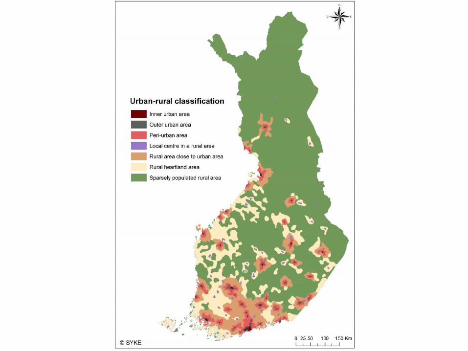
all employed inhabitants in 2011.• New detailed Urban-rural classification by Finnish

Environment Institute SYKE

Data and contextual issues 2/2

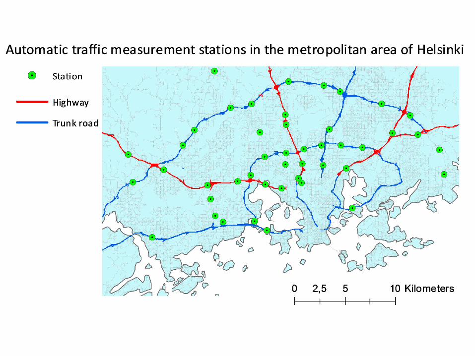
• Traffic sensor data of FTA– Currently 437 stations (vehicle detection loops)

giving information for speed, direction, length and class of a passing vehicle. Target here: speed of passenger cars excluding heavy vehicles.

– Open data services available as well (Digitraffic)

Travel-time model

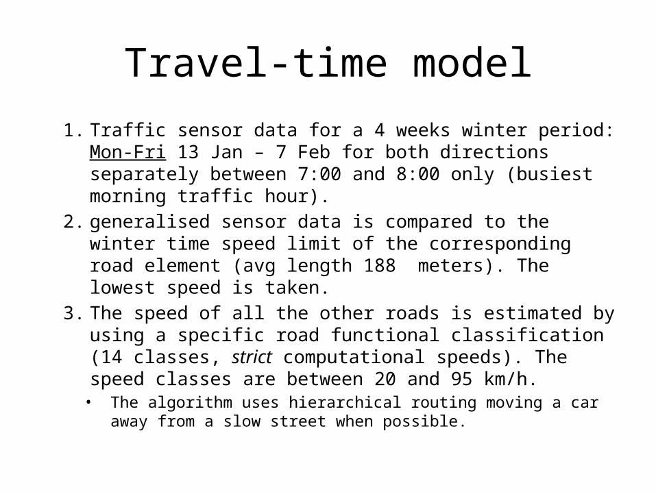
1. Traffic sensor data for a 4 weeks winter period: Mon-Fri 13 Jan – 7 Feb for both directions separately between 7:00 and 8:00 only (busiest morning traffic hour).

2. generalised sensor data is compared to the winter time speed limit of the corresponding road element (avg length 188 meters). The lowest speed is taken.

3. The speed of all the other roads is estimated by using a specific road functional classification (14 classes, strict computational speeds). The speed classes are between 20 and 95 km/h.• The algorithm uses hierarchical routing moving a car away from

a slow street when possible.

Pairwise computing of commuting times and distances 1/2

• 2.1 million coordinate pairs i: ((xid, yid), (xiw, yiw))• Computational complexity is high– ”takes several weeks”

• ESRI ArcGIS® and Python™– number of available licenses is not high– Network Analyst Route Solver

• Documentation is not satisfactory but it works: common Dijkstra’s algorithm

• with hierarchical routing (6-class functional classification: Class I main road, Class II main road, Regional road etc.)

• impedance attribute is the travel time (of a smallest road element); accumulation attribute is the length of a route.

Pairwise computing of commuting distances 2/2

• The solution: 45,000 pairs of points (90,000 datarows) for one program run. 3 parallel runs per one standard computer. For 2 computers (2 licenses): 270,000 distances in about 3 days.

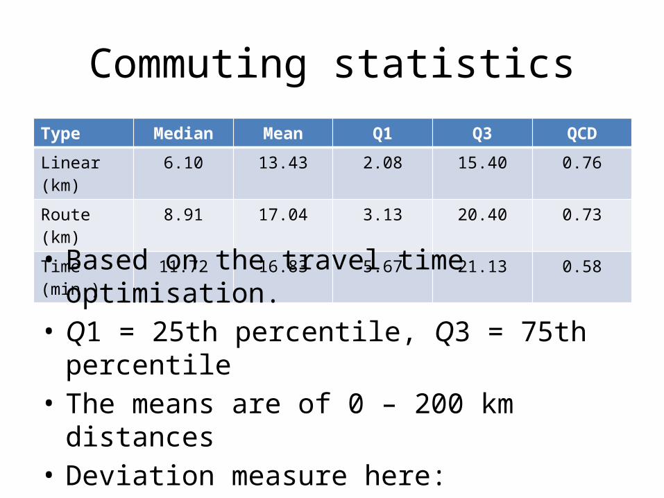
Commuting statisticsType Median Mean Q1 Q3 QCD

Linear (km) 6.10 13.43 2.08 15.40 0.76

Route (km) 8.91 17.04 3.13 20.40 0.73

Time (min.) 11.72 16.83 5.67 21.13 0.58

• Based on the travel time optimisation.• Q1 = 25th percentile, Q3 = 75th percentile• The means are of 0 – 200 km distances• Deviation measure here: • QCD = (Q3 – Q1) / (Q3 + Q1)• Quartile coefficient of dispersion

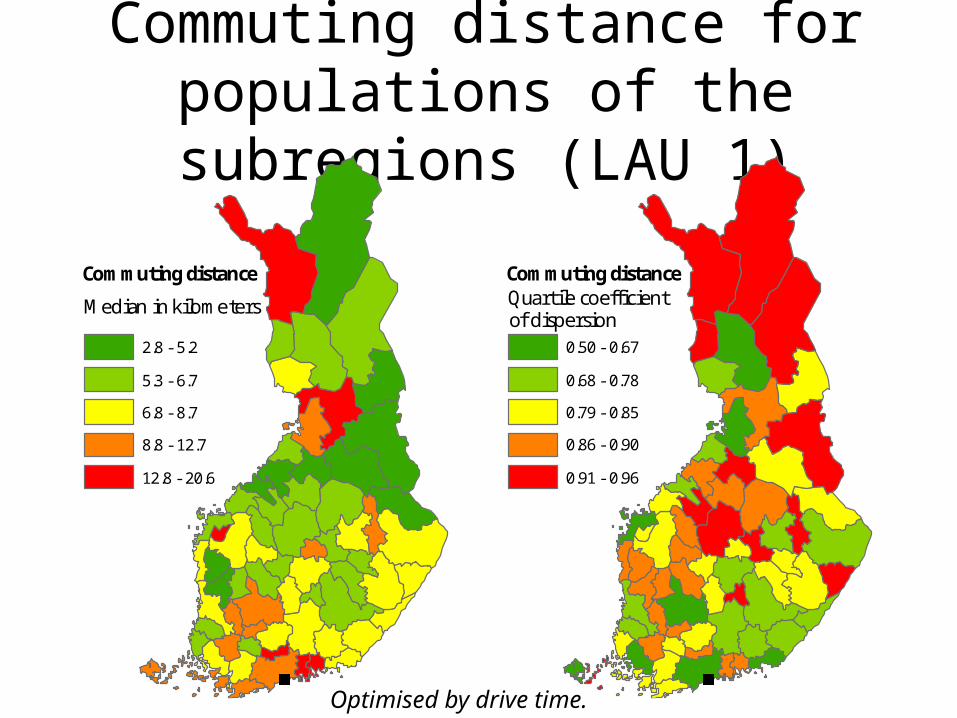
Commuting distance for populations of the subregions (LAU 1)

Commuting distance

Median in kilometers

2.8 - 5.2

5.3 - 6.7

6.8 - 8.7

8.8 - 12.7

12.8 - 20.6

Commuting distanceQuartile coefficientof dispersion

0.50 - 0.67

0.68 - 0.78

0.79 - 0.85

0.86 - 0.90

0.91 - 0.96

Optimised by drive time.

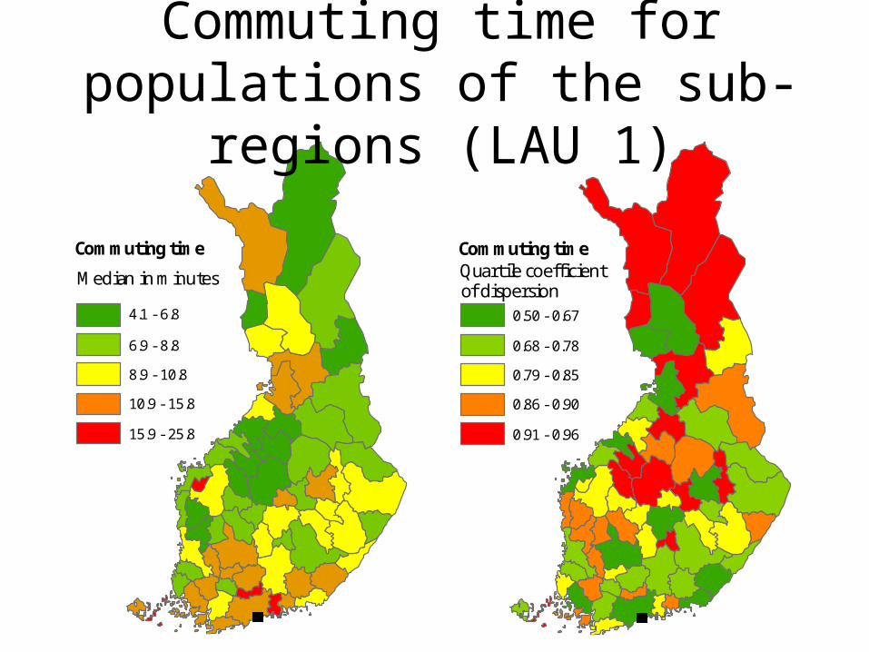
Commuting timeQuartile coefficientof dispersion

0.50 - 0.67

0.68 - 0.78

0.79 - 0.85

0.86 - 0.90

0.91 - 0.96

Commuting time

Median in minutes

4.1 - 6.8

6.9 - 8.8

8.9 - 10.8

10.9 - 15.8

15.9 - 25.8

Commuting time for populations of the sub-regions (LAU 1)

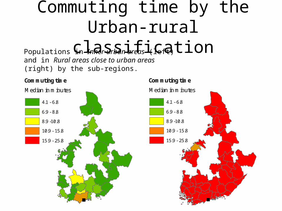
Commuting time

Median in minutes

4.1 - 6.8

6.9 - 8.8

8.9 -10.8

10.9 - 15.8

15.9 - 25.8

Commuting time

Median in minutes

4.1 - 6.8

6.9 - 8.8

8.9 -10.8

10.9 - 15.8

15.9 - 25.8

Commuting time by the Urban-rural classification

Populations in Inner-urban areas (left) and in Rural areas close to urban areas (right) by the sub-regions.

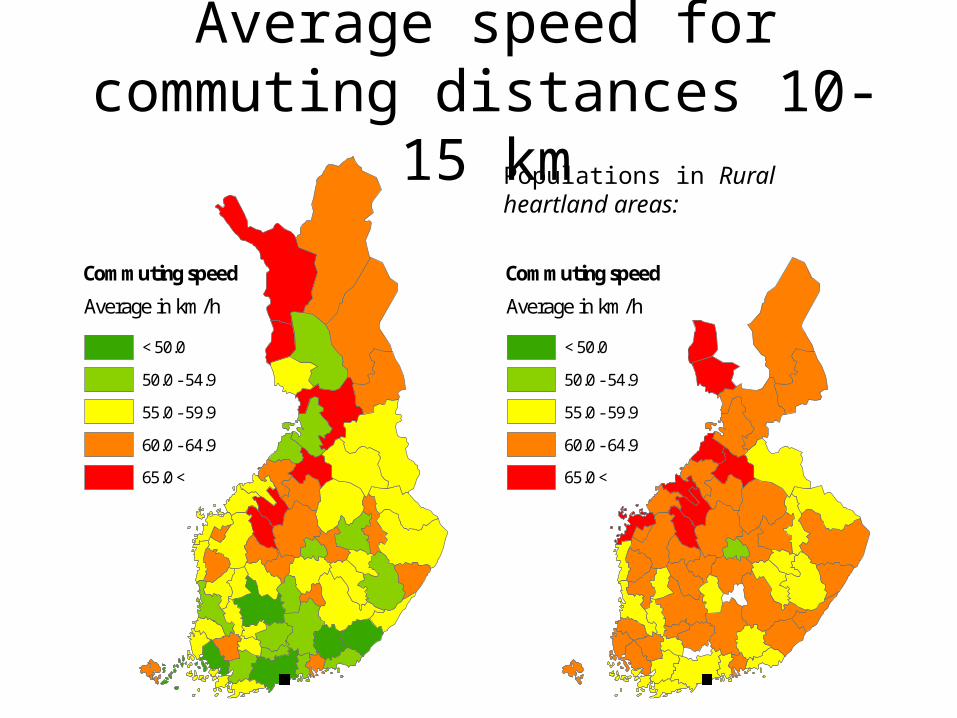
Commuting speed

Average in km/h

< 50.0

50.0 - 54.9

55.0 - 59.9

60.0 - 64.9

65.0 <

Commuting speed

Average in km/h

< 50.0

50.0 - 54.9

55.0 - 59.9

60.0 - 64.9

65.0 <

Average speed for commuting distances 10-15 km

Populations in Rural heartland areas:

Further research and conclusions

• Many accessibility challenges are related to rush hour traffic. The estimation becomes more complex though and might require the help of Big Data.

• The quality of life aspects are relevant in comparison studies: see the conf. paper: 6.1. Time use survey.

• The extensive and detailed national road network will be seen as part of the social statistics data warehouse based applications in forthcoming years.

Dziękuję bardzo za uwagę!pasi.piela@stat.fi