Communication Models for Monitoring Applications …isda.ncsa.uiuc.edu/peter/publications/techreports/2004...Multiple MICA motes form sensor networks, an emerging area of mobile computing

Technical Report: alg04- April 02, 2004

David Scherba, [email protected] Peter Bajcsy, [email protected] Automated Learning Group National Center for Supercomputing Applications 605 East Springfield Avenue, Champaign, IL 61820

Communication Models for Monitoring Applications Using Wireless Sensor Networks Abstract In this paper, we address the problem of efficient, wireless communication between MICA motes and a personal computer. We present four high-level communication models for solving the wireless communication problem in wireless “smart” MEMS sensor networks. We establish the Asynchronous Memory Limited communication model as an effective scheme based on a series of experiments evaluated using a wireless information loss criterion. We provide an overview of lessons learned from previous work, the challenges we encountered, and the different experimental approaches used to evaluate efficiency of wireless communication models. This report presents not only our findings, but also future research directions. 1 Introduction In this paper, we address the problem of efficient, wireless communication between MICA motes and a personal computer. The MICA motes, also known as “smart” micro electro-mechanical systems (MEMS), provide new capabilities for sensing via an on-board processor, on-board storage and wireless communication capabilities. Multiple MICA motes form sensor networks, an emerging area of mobile computing. These networked, “smart” MEMS sensors have the benefits of small size, low cost and low power consumption. While the MICA built-in support for wireless communication makes it possible to deploy them in remote, humanly inaccessible locations, it also raises questions about optimal wireless communication models. The motivation for our work is to explore multiple communication models and to design MICA-based sensor networks using an optimal communication model. This work is primarily driven by our design of a hazard aware space with MICA sensors providing information about the environment to enable proactive control. Examples of proactive control would include (a) fire hazard detection, (b) heating and air-conditioning (HVAC) control and (c) bandwidth-efficient and information-rich video monitoring. In the fire hazard detection application, the wireless sensors are used to detect the presence of a fire (this might be through a combination of different modalities including temperature, visual, and smoke detection). The sensor readings are relayed through a network to a base station, which decides on an action to take (e.g. sounding an alarm, triggering a sprinkler system, dispatching a person (or robot) to investigate, etc…). In the heating/AC control application, the wireless sensors are used as intelligent thermostats. In addition to monitoring their immediate location, the sensors can communicate with each other (and a possible base station) to determine and carry out an optimal heating/cooling strategy. In the last example, a wireless sensor network is used to provide in situ measurements of physical quantities. MICA on-board processing of in situ measurements can

Communication Models for Applications Using Wireless Sensor Networks

2

trigger video monitoring thus saving communication bandwidth. In order to increase information value of spectral video, imagery can be calibrated with the sensor measurements (e.g., thermal infrared video) thus providing information for accurate hazard detection. We have described and designed a thermal infrared camera calibration system using MICA motes in our past work [8]. For this report, we define optimality in terms of system information loss. We define information loss as:

( ) ( )

( ) ( )

# sensor readings receivedinformation loss 1 *100%

# sensor readings# sensors timesensor time

= −

⋅

(1)

Note that information loss includes the inherent loss of sensor data when the sensor is not collecting data. The optimal communication model is the one which minimizes system information loss from a MICA sensor network and a base station (attached to a personal computer). While searching for the optimal communication model with minimum information loss, we assume that there are three major components determining the information loss: (1) hardware, e.g., the antenna design and physical communication protocol, (2) software environment, e.g., the TinyOS communication stack, and (3) wireless network environment, for example, the presence of other wireless devices, propagation media and the topography of the physical environment.

There has been significant research on network communication schemes in [9], [10], [11], [12], [15] and [17]. Many “throughput” issues have been addressed at a low level (i.e. the media access control (MAC) layer) and with different network assumptions. A survey of MAC schemes for wireless networks is given in [9]. More thorough mathematical treatments can be found in [12], [15], and [17]. MAC schemes designed for the constraints of wireless sensor networks (e.g. low power) have been researched in [10] and [11]. When using a protocol stack (e.g. TCP/IP, or TinyOS’s active messages), higher level protocol or design choices [possibly in combination with lower levels of the stack] can affect system performance. In the case of TCP/IP, researchers have investigated modifications to TCP to improve performance characterized by papers like [18]. Modifications (usually to lower levels of protocol stacks) to increase system throughput have been considered in the mobile multimedia arena in [19] and [20].

Our communication models are most similar to the approaches in [19] and [20]. The difference, aside from the application space, is that in [20] the lower layer (the MAC scheduling protocol in [19]) is modified, whereas we modify the application layer (keeping the MAC layer as an invariant). Our reasoning for this choice is that the MAC layer of TinyOS is currently quite volatile: it has changed before, often to accommodate different radios, and will change again in the near future. We wished to concentrate our efforts on an approach that might outlast a single version of TinyOS. There are potential gains to be had from considering both low and high level modifications jointly. We leave this as an area of future research.


3

We have reported evaluation of two communication models in our past work, [8], that were termed “autosend” and “query” (similar to the traditional “interrupt” and “polling” interface techniques). Since “query” did not fare very well in [8], we only chose to use the “autosend” communication model for comparison purposes. The other three communication models are the Autosend Communication Model, the Synchronous Memory Limited Communication Model, the Synchronous Memory Demanding Communication Model, and the Asynchronous Memory Limited Communication Model. Section 2 breaks down the MICA communication system components in detail. Section 3 proposes a set of high-level communication models which can be implemented on the MICA communication system. Section 4 discusses our communication model experiments and our results. Section 5 summarizes our results and concludes with directions for future research. We include an appendix with some general information on programming MICA sensors along with solutions to implementation-specific problems we faced. 2 Communication System Components The MICA communication system can be broken down into three components. Section 2.1 discusses the sensor hardware. Section 2.2 details the MICA software environment. The external network environment is discussed in section 2.3. 2.1 Hardware Description - MICA Wireless Smart Sensor This section describes the MICA Wireless Smart Sensor. It gives the sensor specifications and some details of the software suite used to program the sensors. In this report, we will use the term mote and sensor node interchangeably. ‘Mote’ is a commonly used term in the wireless sensor literature literally meaning “a small particle1.” 2.1.1 Sensor specification In order to understand the capabilities and limitations of the MICA motes, we need to know the specifications of the sensors [1]. The sensors that we used for this study were bought from Crossbow Technology Inc. [2]. The MICA motes come in two parts: a processor/radio board and add-on sensor boards. This paper only discusses issues related to the former, although the latter is used to generate data. For this paper, we used the MPR300CB [3] processor/radio board (reference Figure 1 and Figure 2). The MPR300CB specifications are: (1) 4MHz Atmega 128L Processor (2) 128KB Flash, 4KB SRAM, 4KB EEPROM (3) 916MHz TR1000 [4] radio transceiver with a maximum [theoretical] data rate of 40Kbps (4) Powered by 2 AA batteries

1 mote is also used jokingly to refer to the vision of the wireless smart sensors approaching the scale of dust versus the current state of the art


4

Figure 1 Picture of MICA1 (left) and MICA2 (right) Processor/Radio Boards

Figure 2 Block Diagram of MICA Processor/Radio Board

A MICA mote currently costs (depending on the set of sensors attached to it) about 100 – 300 US dollars and is approximately 4 inches by 2 inches by 1 inch in size. The computational, communication and sensing features together with the low cost and size make these wireless smart sensors a very attractive alternative to their traditional counterparts. However, all the above capabilities have severe limitations. Sensors have limited processing and storage capability. Moreover, since AA batteries supply power to sensors, power becomes an expensive commodity. These limitations heavily influence any sensor application design and will be discussed in detail later. 2.2 Software Environment Sensors are programmed with a programming board interfaced to a personal computer via a parallel port. MICA motes are programmed using TinyOS [6], an open source software platform developed by researchers at UC Berkeley and actively supported by a large community of users. It is a small operating system that allows networking, power management and sensor measurement details to be abstracted from core application development. TinyOS is optimized for efficient computational, energy and storage usage. The key to TinyOS’s functionality is the NesC (network-embedded-systems-C) compiler, which is used to compile TinyOS programs. NesC has a C like structure and provides several advantages such as interfaces, wire error


5

detection, automatic document generation, and facilitation of significant code optimizations. One of its major goals is to make TinyOS code cleaner, easier to understand, and easier to write. TinyOS consists of a tiny scheduler and a graph of components [7]. A component has a set of ‘command’ and ‘event’ handlers. An event is like an interrupt sent from one component to another informing that something of interest to the receiver has occurred. For example, once an application’s component has set the Timer component for a particular interval, the Timer component will inform the application through the ‘Timer.fired()’ ‘event’, when the specified interval is over. Conversely, a component can invoke another component’s functionality using the called component’s ‘command’ interface. An application would be using the command ‘setTimer()’ of the Timer component to use the timer functionality. This clean abstraction allows for rapid code development. Application development involves connecting your components to already implemented components and specifying how they will be linked to each other, that is, which component will invoke which command and which component will signal another component’s events. This linkage is specified in a configuration file, which is one of the two files for any TinyOS component. The other file is the module file which contains the actual code for an application. Writing code is fairly simple if one has some basic knowledge of C programming. In order to perform longer processing operations, TinyOS introduces a scheduling hierarchy consisting of ‘tasks’ and ‘events’. Tasks are used to perform longer processing operations, such as background data processing and can be preempted by events. However, one task cannot preempt another task. Thus, a task should not spin or block for long periods of time. If one needs to run a series of long operations, one should have a separate task for each operation. Events are usually used to perform responses to interrupts and can be preemptive. Having preemptive code (with shared data) admits the possibility of race conditions. The TinyOS atomic statement provides a foundation for synchronization. Keeping energy conservation in mind, the processor has three sleep modes: ‘idle’ which just shuts the processor off; ‘power down’, which shuts everything off except the watch-dog; and ‘power save’, which is similar to power-down, but leaves an asynchronous timer running. Power consumption equates to battery life. Long battery life is desired, and in some applications, one to five years is required. The processors, radio, and a typical sensor load consume a power of about 100mW. This figure should be compared with the 30 µW drawn when only the 32 kHz timer (and some other essential electronics) are running (power-save mode). When using power management (provided by TinyOS), the mote will automatically enter the power-save state when it can. The mote will switch into an active state on the next 32 kHz timer interrupt ready to resume processing. Therefore, an energy-efficient system must embrace the philosophy of getting work done in small, contiguous time periods (i.e. as quickly as it can) and sleeping for the remainder of the time. While writing application code, care must be taken in terms of power, CPU and memory usage. One should avoid writing very complex programs. The TinyOS architecture and scheduling policies must be kept in mind to write ‘efficient’ and ‘correct’ code. Careful planning and coding


6

will lead to better application development and deployment. The appendix presents a troubleshooting guide covering some specific problems we faced during our work on the sensors. 2.3 Network Environment The network environment has a drastic effect on system information loss, but it is the hardest to control. We consider the network environment to include radio frequency (RF) propagation issues (i.e. the choice and antenna type and parameters, the antenna orientation and location, the propagation medium, and the surrounding propagation obstacles), as well as possible interference due to wireless devices operating at similar frequency or other frequencies. There exist a few theoretical models for predicting antenna radiation amplitude patterns under a set of specific assumptions [23]. For example, if we assume an infinitesimal horizontal or vertical electric dipole above an infinite electric conductor (antenna type: dipole, orientation: horizontal or vertical with respect to ground) and no propagation obstacles, then the amplitude radiation patterns will become more homogeneous with larger elevation about the ground (see [23], Section 7.4). More accurate approximations of straight wire antenna type require more complex models that incorporate the fact that the antenna has a finite length and is formed by a cylinder. Other types of antennas, such as, strips, conducting wedges or spheres, can also be modeled with complex models as documented in [23], Chapter 11. We investigated the effect of RF interference in the past [8]. In short, wireless phones (operating in the same 900MHz band as the sensor network) proved to be the only major impediment to sensor communication. In this document, we have only investigated (and run our experiments) on sensor networks located inside our office building (i.e. in air with “office” interference including PC’s, wireless networking, and wireless communication devices). We have conducted a few empirical experiments with multiple antenna shapes and antenna orientations. Our experiments were conducted by measuring information loss over a period of 1 minute between a single mote and base station placed 100” apart. We have only tested antenna configurations for the MICA processor/radio boards as the MICA2 processor/radio boards are quite different. Specifically, the MICA2 uses a very different radio (a Chipcon CC1000 [5]) and uses a MMCX connector for the antenna. The latter currently limits our antenna choice to the provided straight wire antennas furnished with a loop (see http://www.xbow.com/Products/productsdetails.aspx?sid=61), although other antennas are available. For instance, a larger directional antenna (with MMCX connector) could easily be connected to a MICA2 in applications needing increased range (at the cost of size). In a single wire antenna design, there are three variables, namely, wire length, shape and orientation. The desired wire length can be computed according to the following formula: 75/frequency(MHz) = length in meters. Based on this formula, the recommended antenna length is a 8.2 cm for 916MHz and 17.3 cm for 433MHz. Other researchers reported tests with a 3.5” (3.5*2.54=8.89cm) long antenna [22]. In terms of the antenna material, it is suggested to use solid copper (see http://webs.cs.berkeley.edu/tos/hardware/design/ORCAD_FILES/MICA/antenna.html). One of the commercially available antennas satisfying the above criteria and hence suitable for MICAs is a Linx Technologies JJB series ¼ wavelength antenna (see


7

http://www.linxtechnologies.com/ldocs/antennas/m_antjjb.php3). This particular antenna is a quarter wavelength whip, coiled into a helix, and embedded in a plastic can. In our experiments, we used (a) a straight wire of length 8.2 cm, (b) a coiled wire of length 8.2 cm, and (c) no antenna. The diameter of the coils in (b) was set to 0.27” to match the coil dimension of the Linx Technologies antenna. Antenna orientation was the only other variable in our experiments. Common to all experiments were two motes (the first programmed with PhotoTemp_Test, the other programmed with TOSBase and connected to a laptop computer). The motes were placed 100” apart along a hallway (i.e. they had direct line-of-sight). Our preliminary testing determined that the TOSBase mote should have its antenna pointing straight upward (orientations along the floor resulting in major packet loss). We also determined that the PhotoTemp_Test mote performed best on its side (the circuit board facing the direction of the TOSBase mote) elevated from above the floor on an inverted paper cup (approximately 5”). Information loss over a period of 1 minute was used as a metric. Given the preceding invariants, Figure 3 illustrates one of the configurations of antennas and Table 1 summarizes our overall results.

Figure 3. One configuration of antennas with a coiled antenna on the MICA mote (left) and a straight antenna at the TOSbase station (right).

Table 1. A summary of a set of experiments with varying shape and orientation of MICA antennas.

Antenna Type/Orientation

Number of Missing Readings

Number of Correct Readings

Total Number of Readings

Information Loss

None 20 1200 1220 1.64% Straight, Up (normal to circuit board)

0 1220 1220 0%

Straight, Along short side of circuit board

10 1210 1220 0.82%

Straight, Along long side of circuit board

170 1050 1220 13.93%


8

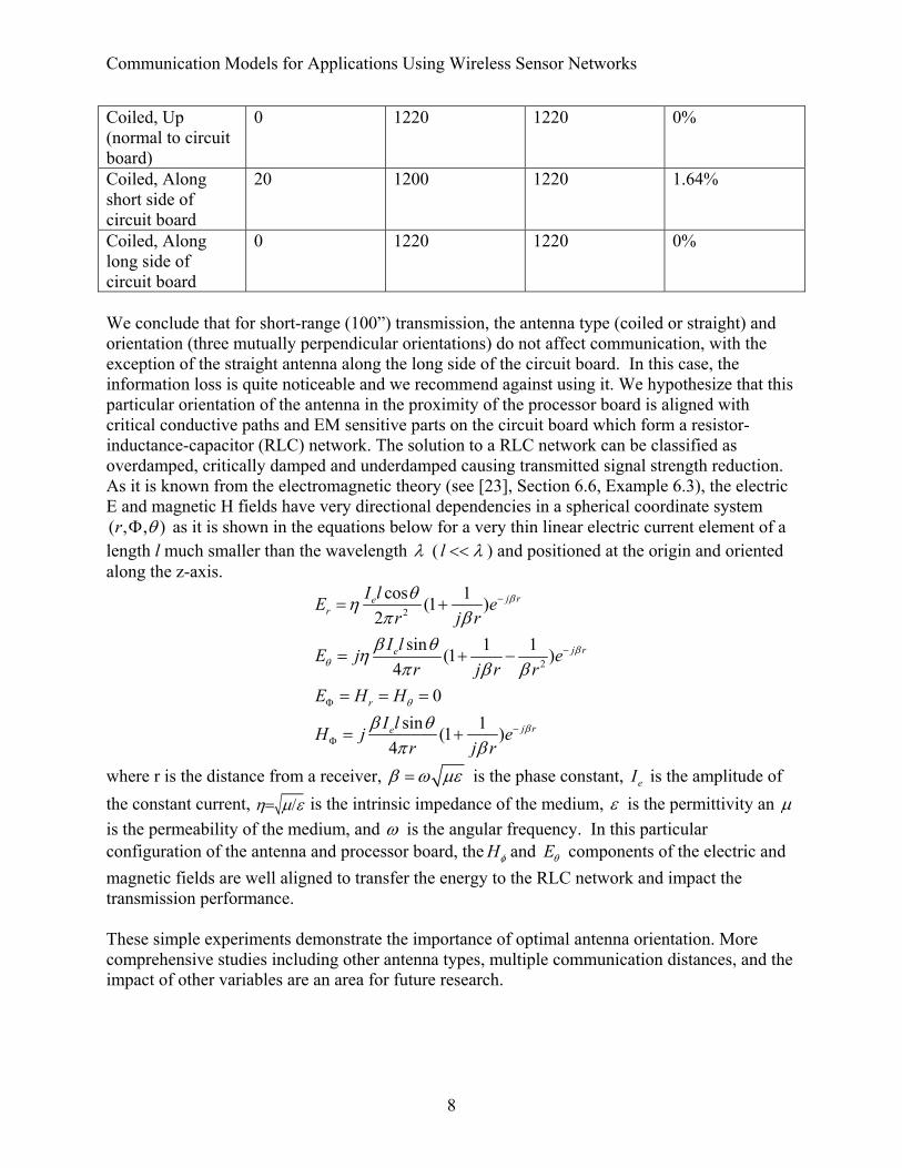
Coiled, Up (normal to circuit board)

0 1220 1220 0%

Coiled, Along short side of circuit board

20 1200 1220 1.64%

Coiled, Along long side of circuit board

0 1220 1220 0%

We conclude that for short-range (100”) transmission, the antenna type (coiled or straight) and orientation (three mutually perpendicular orientations) do not affect communication, with the exception of the straight antenna along the long side of the circuit board. In this case, the information loss is quite noticeable and we recommend against using it. We hypothesize that this particular orientation of the antenna in the proximity of the processor board is aligned with critical conductive paths and EM sensitive parts on the circuit board which form a resistor-inductance-capacitor (RLC) network. The solution to a RLC network can be classified as overdamped, critically damped and underdamped causing transmitted signal strength reduction. As it is known from the electromagnetic theory (see [23], Section 6.6, Example 6.3), the electric E and magnetic H fields have very directional dependencies in a spherical coordinate system ( , , )r θΦ as it is shown in the equations below for a very thin linear electric current element of a length l much smaller than the wavelength λ ( l λ<< ) and positioned at the origin and oriented along the z-axis.

2

2

cos 1(1 )2

sin 1 1(1 )4

0sin 1(1 )

4

j rer

j re

r

j re

I lE er j r

I lE j er j r r

E H HI lH j e

r j r

β

βθ

θ

β

θηπ ββ θη

π β β

β θπ β

−

−

Φ

−Φ

= +

= + −

= = =

= +

where r is the distance from a receiver, β ω µε= is the phase constant, eI is the amplitude of the constant current, /η µ ε= is the intrinsic impedance of the medium, ε is the permittivity an µ is the permeability of the medium, and ω is the angular frequency. In this particular configuration of the antenna and processor board, the Hφ and Eθ components of the electric and magnetic fields are well aligned to transfer the energy to the RLC network and impact the transmission performance. These simple experiments demonstrate the importance of optimal antenna orientation. More comprehensive studies including other antenna types, multiple communication distances, and the impact of other variables are an area for future research.


9

3 Proposed Communication Models We propose four communication models designed for applications running on TinyOS 1.0.0 and TinyOS 1.1.02. The models are described and depicted in the following sections. None of the following models are “reliable” in the sense of wireless packet loss. Many network protocols (e.g. TCP) are reliable in this way, but reliability comes at a cost. Specifically, the nodes implementing a reliable protocol must track whether data is corrupted (usually by using a CRC or checksum mechanism), and whether sent data has been received (by the use of acknowledgements). These considerations add computation and network use to a system (which implies the use of extra power). The benefit of reliable communication is that all sent data is received. In our experimentation, we have found very little evidence of packet corruption or loss (loss that does occur appears to be due to data overload in a sensor causing it to overwrite a buffer). We feel that the cost of implementing a reliable model exceeds the cost of data loss in our applications (more data will always come, and it will probably be more relevant to any real-time application than the old/lost data). Adding in reliability to the following models can certainly be done, however, and reliable communication model performance is left as an area of future research.

2 More specifically, the models we propose assume MAC layer behavior identical to TinyOS 1.0.0. The MAC layer used in TinyOS 1.0.0 is similar to Multiple Access with Collision Avoidance (MACA) [16], but is unique to TinyOS. This MAC layer is assumed throughout this paper.


10

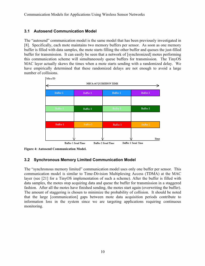
3.1 Autosend Communication Model The “autosend” communication model is the same model that has been previously investigated in [8]. Specifically, each mote maintains two memory buffers per sensor. As soon as one memory buffer is filled with data samples, the mote starts filling the other buffer and queues the just-filled buffer for transmission. It can easily be seen that a network of [synchronized] motes performing this communication scheme will simultaneously queue buffers for transmission. The TinyOS MAC layer actually skews the times when a mote starts sending with a randomized delay. We have empirically determined that these randomized delays are not enough to avoid a large number of collisions.

Figure 4: Autosend Communication Model.

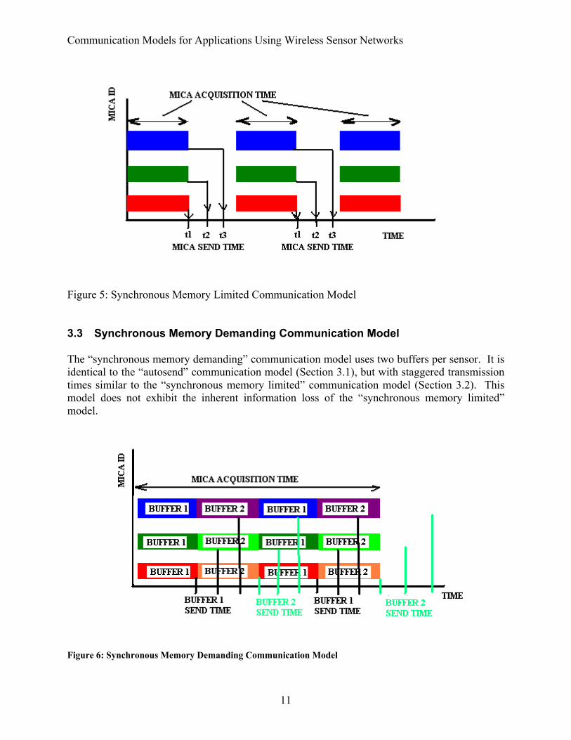
3.2 Synchronous Memory Limited Communication Model The “synchronous memory limited” communication model uses only one buffer per sensor. This communication model is similar to Time-Division Multiplexing Access (TDMA) at the MAC layer (see [21] for a TinyOS implementation of such a scheme). After the buffer is filled with data samples, the motes stop acquiring data and queue the buffer for transmission in a staggered fashion. After all the motes have finished sending, the motes start again (overwriting the buffer). The amount of staggering is chosen to minimize the probability of collision. It should be noted that the large [communication] gaps between mote data acquisition periods contribute to information loss in the system since we are targeting applications requiring continuous monitoring.


11

Figure 5: Synchronous Memory Limited Communication Model 3.3 Synchronous Memory Demanding Communication Model The “synchronous memory demanding” communication model uses two buffers per sensor. It is identical to the “autosend” communication model (Section 3.1), but with staggered transmission times similar to the “synchronous memory limited” communication model (Section 3.2). This model does not exhibit the inherent information loss of the “synchronous memory limited” model.

Figure 6: Synchronous Memory Demanding Communication Model


12

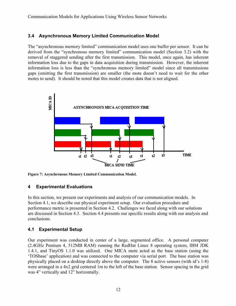
3.4 Asynchronous Memory Limited Communication Model The “asynchronous memory limited” communication model uses one buffer per sensor. It can be derived from the “synchronous memory limited” communication model (Section 3.2) with the removal of staggered sending after the first transmission. This model, once again, has inherent information loss due to the gaps in data acquisition during transmission. However, the inherent information loss is less than the “synchronous memory limited” model since all transmissions gaps (omitting the first transmission) are smaller (the mote doesn’t need to wait for the other motes to send). It should be noted that this model creates data that is not aligned.

Figure 7: Asynchronous Memory Limited Communication Model.

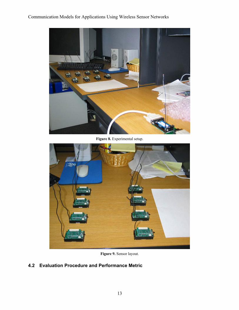
4 Experimental Evaluations In this section, we present our experiments and analysis of our communication models. In Section 4.1, we describe our physical experiment setup. Our evaluation procedure and performance metric is presented in Section 4.2. Challenges we faced along with our solutions are discussed in Section 4.3. Section 4.4 presents our specific results along with our analysis and conclusions. 4.1 Experimental Setup Our experiment was conducted in center of a large, segmented office. A personal computer (2.4GHz Pentium 4, 512MB RAM) running the RedHat Linux 8 operating system, IBM JDK 1.4.1, and TinyOS 1.1.0 was utilized. One MICA mote acted as the base station (using the ‘TOSbase’ application) and was connected to the computer via serial port. The base station was physically placed on a desktop directly above the computer. The 8 active sensors (with id’s 1-8) were arranged in a 4x2 grid centered 1m to the left of the base station. Sensor spacing in the grid was 4” vertically and 12” horizontally.


13

Figure 8. Experimental setup.

Figure 9. Sensor layout.

4.2 Evaluation Procedure and Performance Metric


14

The motes were programmed with each communication scheme in turn and each mote was assigned one of the ids/addresses from 1 to 8. The ‘oscope_autosend_1’ (modified ‘oscilloscope’ program) was used to initiate, stop, and calculate “packet loss” statistics. Data collection was performed by a personal computer (PC) connected to a base station with a RF receiver. The data collection interval was 60 seconds (timed with a watch). All output files were saved to the hard drive of the PC in directories corresponding to the TinyOS “application” implementing the communication scheme: Table 2: Descriptions of four communication schemes and their tinyOS application names.

Application Name Communication Scheme Description PhotoTemp_Test Raw autosend (two buffers, no delays beyond

those in the MAC layer) PhotoTemp_SyncMemDeman Synchronous Memory Demanding (two buffers

with delays inserted to minimize collisions) PhotoTemp_SyncMemLimit Synchronous Memory Limited (one buffer

always starting at the same time with delays inserted)

PhotoTemp_AsyncMemLimit Asynchronous Memory Limited (one buffer with skewed sends the first time, and no delays after that)

Information loss was calculated according to Equation (1) in Section 1.


15

Figure 10. Screenshot of ‘oscope_autosend_11’ Program.

4.3 Implementation Challenges We ran across a number of challenges while implementing the four communication models for MICA motes running TinyOS 1.1.0. The following sections detail the problems and our solutions. 4.3.1 Synchronization in TinyOS Our goal for our experiments was to collect data from two sensors (e.g. the photosensor and the thermocouple) on each mote at the same time (think of the preceding models as having two identical swaths for each mote). TinyOS, by way of tasks, serializes per-mote transmission. TinyOS does not provide a mechanism to ensure that [two] events have happened before engaging the transmission of data. Without such a mechanism, there is the potential that old, or random, bits might be sent as sensor data. Many operating systems offer synchronization primitives to handle these situations.


16

We chose to create our own barrier synchronization primitive (utilizing TinyOS’s atomic statement to prevent deadlock). We implemented “barrier” in “Barrier.nc” and “BarrierM.nc” and used it in all of the above communication models. The general idea is that all relevant threads of execution must reach the barrier before any thread can pass. Our implementation signals an event upon arrival of the last thread, which starts the transmission process. 4.3.2 “Stagger” Interval Determination In the above communication models, there are often delays that are used to stagger data transmission. The delays are fundamentally designed to equal the time it takes to send one mote’s sensor datum. This number (in timer ticks) was computed using the following formula:

(# )*( ) ( & )bits in packet timer tick(#of sensors) ( )

sensor 40 bits

delay bits to send effective transmission speed OS MAC layer uncertainty

uncertainty factor

= + =

= +(2)

The uncertainty factor is set to handle system-level issues as well as the effect of delays in the MAC layer: it is set empirically to minimize the information loss. One tick worked well in our experimentation. In models like “synchronous memory limited,” the actual delay is a multiple of the above number (the multiples due to waiting for multiple sensors to send). 4.3.3 Granularity of the Counter The final challenge we faced was in updating packet counters for use in information loss measurements. The counters are integer values (for a number of reasons), but often delays in timing needed to be expressed in non-integer amounts (e.g. 0.46). We handled this by an engineering approximation. In the above example, we incremented the counter by 1 every two events (effectively giving increments of 0.5). This was a conservative approximation for our application, ensuring that reality is at least as good as we report. 4.4 Measured Experimental Results Table 3: Measured information loss for the evaluated four communication models.

Communication Model

Number of Missing Readings

Number of Correct Readings

Total Number of Readings

Information Loss

Raw Autosend 3560 6150 9710 36.7% Synchronous

Memory Demanding

980 8770 9750 10.1%

Synchronous Memory Limited

4157 5390 9547 43.5%

Asynchronous Memory Limited

230 8890 9120 2.5%


17

When comparing the statistics listed in Table 3, one should consider several critical variables that change values of these statistics. First, the environment (especially the RF environment) is difficult to control. A large number of trials could be conducted and the results averaged to mitigate this factor. We have conducted four experiments with similar results (the above data is from the second experiment). We believe that these four experiments give repeatable and representative statistics of real-world performance of these communication models. Second, timing on the MICAs is still a thorny issue for a number of reasons. The statistics listed above are calculated in the “oscilloscope” program using counters from the motes. These counters are incremented by events triggered by timer interrupts. In addition to the quality of the MICA timer, the state of the system can have a drastic effect (e.g. the counter-update routine can itself be interrupted). Additionally, in the Synchronous Memory Limited and Asynchronous Memory Limited cases, the counter needs to be incremented by a fractional amount (theoretically around 0.46) in order to give accurate numbers. This increment is non-trivial given the software architecture, so the current implementation increments the counter by 1 every two ticks (i.e. it averages out to 0.5: an engineering approximation on the conservative-side). Gains in timing accuracy do not help the schemes perform better, so we ended our investigation into timing accuracy at this point. By inspecting the results, we concluded that the Asynchronous Memory Limited communication model performs significantly better than the competition. We believe the primary reason for this is that the model only has inherent information loss at the start in conjunction with a minimal number of network collisions. In fact, over time the inherent information loss approaches 0%. Every other model we consider has either larger inherent losses, or [apparently] a large number of network collisions. At first, we theorized that the large number of network collisions was a result of picking a bad stagger interval, but changing the interval did not improve the results. This suggests that other factors (e.g. the initial [random] MAC delay on a packet send and OS scheduling “jitter”) might drag real-world performance. We conclude that the Asynchronous Memory Limited communication model is the most optimal communication model among the four proposed models. 5 Summary and Directions for Future Research We do not see too much room for improvement in the TinyOS application-domain alone. Further improvements in information throughput will likely come by modifying the “kernel” of TinyOS, specifically the MAC layer. There has been some limited work toward this goal, for instance, a group at Virginia has implemented a TDMA-based MAC layer [21], and the TinyOS project has released an updated MAC layer as well. Further gains can possibly be made by attempting to optimize the network stack and application-level communication scheme jointly. Information throughput gains can be made in these areas because the traditional network assumptions do not hold. Specifically, in many applications, the sending times/behavior of all network entities are known a priori. The results reported in this paper are specific to TinyOS 1.1 running on MICA motes. We believe that our conclusions should be applicable to wireless sensor networks with similar


18

[single-hop] topology, limited number of nodes, and a similar MAC layer. The TinyOS MAC layer is slated for replacement, so more research may need to be done to establish similar results. Our conclusions are that “system loss” can be improved by modifying the communication scheme. Our results indicate that the Asynchronous Memory Limited approach is the best way to minimize system loss among the four communication models evaluated in this work.


19

6 References [1] Crossbow Technology, Inc. MICA Sensor Brochure, http://www.xbow.com/Products/Product_pdf_files/Wireless_pdf/MICA.pdf. [2] Crossbow Technology, Inc., http://www.xbow.com. [3] Crossbow Technology, Inc. Sensor Manual, http://www.xbow.com/Support/Support_pdf_files/MTS-DA_Series_User_Manual_RevB.pdf [4] RF Monolithics, Inc. TR1000 Datasheet, http://www.rfm.com/products/data/tr1000.pdf. [5] Chipcon CC1000 Datasheet, http://www.chipcon.com/files/CC1000_Data_Sheet_2_1.pdf. [6] TinyOS Official Website, http://www.tinyos.net/. [7] TinyOS Tutorial, http://www.tinyos.net/tinyos-1.x/doc/tutorial/, [8] S. Saha and P. Bajcsy. “System Design Issues for Applications Using Wireless Sensor Networks,” NCSA Technical Report, http://algdocs.ncsa.uiuc.edu/TR-20030823-1.doc. [9] A.C.V. Gummalla and J.O. Limb. “Wireless Medium Access Control Protocols.” IEEE Communications Surveys, http://www.comsoc.org/livepubs/surveys/public/2q00issue/gummalla.html. [10] C.S. Raghavendra and S. Singh, “PAMAS–Power Aware Multi-Access protocol with Signalling for Ad Hoc Networks,” ACM SIGCOMM Computer Communication Review, vol. 28, no. 3, July 1998, pp. 5-26. [11] W. Ye, J. Heidemann and D. Estrin, “An Energy-Efficient MAC protocol for Wireless Sensor Networks,” Proc. 21st Joint Conf. IEEE Computer and Comm. Societies (INFOCOM 2002), IEEE, vol. 3, issue 2003, pp 1567-1576. [12] R. Rom and M. Sidi. Multiple Access Protocols: Performance and Analysis. Springer-Verlag, 1990. [13] J. Elson and D. Estrin, “Time Synchronization for Wireless Sensor Networks,” Proc. 2001 International Parallel and Distributed Processing Symposium (IPDPS), 2001. [14] J. Elson, L. Girod and D. Estrin. “Fine-Grained Network Time Synchronization using Reference Broadcasts”. Submitted for review, February 2002. [15] L. Kleinrock and R. Tobagi, “Packet Switching in Radio Channels: Part I--Carrier Sense Multiple-Access Modes and their Throughput-Delay Characteristics,” Communications, IEEE Transactions on, vol. 23, no. 12, Dec 1975, pp 1400-1416. [16] P. Karn, “MACA - A New Channel Access Method for Packet Radio,” Proc. of the 9th ARRL Computer Networking Conference, London, Ontario, Canada, 1990. [17] S. S. Lam. “A carrier sense multiple access protocol for local networks.” In Computer Networks, volume 4, pages 21 – 32, 1980. [18] J. Mo, R. J. La, V. Anantharam, and J. Walrand, “Analysis and Comparison of TCP Reno and Vegas,” Proc. 18th Joint Conf. IEEE Computer and Comm. Societies (INFOCOM 1999), IEEE, vol. 3, pp 1556 – 1563. [19] A. Baiocchi and F. Vacirca, “End-to-End Evaluation of WWW and File Transfer Performance for UMTS-TDD,” Proc. Global Telecommunications Conference, 2002 (GLOBECOM 2002), IEEE, vol. 1, pp 737-741. [20] M. Malkowski and S. Heier, “Interaction between UMTS MAC Scheduling and TCP Flow Control Mechanisms,” Proc. Int. Conf. on Comm. Technology (ICCT 2003), IEEE, vol. 2, pp 1373 – 1376.


20

[21] L. Gu, “PRIME: A Collision-Free MAC Protocol,” Draft, http://www.cs.virginia.edu/~lg6e/MAC.pdf. [22] S. Klemmer, S. Waterson, and K. Whitehouse, “Towards a Location-Based Context-Aware Sensor Infrastructure,” CS Division, EECS Department, University of California at Berkeley, December 2000. accessible at URL: http://guir.berkeley.edu/projects/location/Location.pdf [23] C.A. Balanis, Advanced Engineering Electromagnetics, John Wiley and Sons, New York, N.Y., 981 p., 1989.


21

7 Appendix This appendix covers specifics of programming MICA motes along with problems we have faced (and their solutions). It is our hope that this supplementary knowledge will be of use to a reader. For more detailed information, including a step-by-step tutorial, reference [6] and [7]. 7.1 Programming the motes In order to program a MICA mote with an application, follow the steps given below: (1) On the computer configured with TOS tools, compile the TinyOS application code that you want to program your mote with. If you have successfully installed TinyOS then if are in the directory where the code resides, typing “make mica” compiles the code. (2) Place the mote board (or the mote and sensor stack) into the bay on the programming board. In order to program a board, one must supply a 3-volt supply to the connector on the programming board or power the node directly. The red LED on the programming board will be on when power is supplied. (3) Plug the 32-pin connector on the programming board into the parallel port on the computer that has the TinyOS installed, using a standard parallel port cable. (4) Type: “make mica install”. This should install the code on the mote. If you want to designate an identification number (ID) of the mote, type the ID number after install. For example, typing “make mica install.2” will assign an ID of 2 to the mote. 7.2 Generating documents for debugging A useful feature in TinyOS is that it allows you to generate documentation on the fly, during code compilation. The document thus generated gives a pictorial representation of how the different components used by the code are wired to each other. This can be very helpful during debugging as it allows the programmer to ensure that the components are linked as intended by the programmer. One can generate the document for a code by typing: “make docs mica” for compiling the code instead of typing “make mica”. 7.3 Motes programmed without errors, but not giving the desired output? Before you do anything else, make sure you know your sensors and Mica board well (http://webs.cs.berkeley.edu/tos/tinyos-1.x/doc/micasbl.pdf) and have checked some of the files that are used during installation of your program on the motes. One such file is the Makerules file in the tinyos-1.x/apps directory. By default, when we say ‘make mica install’ while programming our motes, Makerules file assumes that the mica board is of type ‘micasb’. However, as we found out later, after a few weeks of futile effort at programming our motes to give the right output, our motes were of type ‘basicsb’. To get the right output, we then changed the following Makerules file’s lines:

#Sensor Board Defaults


22

ifeq ($(SENSORBOARD),) ifeq ($(PLATFORM),mica)

# SENSORBOARD = micasb …comment this out SENSORBOARD = basicsb …add this line endif endif

If you are sure that the problem is not in your code, and that all the components are wired well in your code’s configuration file, then you should check the other ancillary tinyos files to ensure that the right setting are being used. Directory contents of ‘tinyos-1.x\tos\sensorboards’ give the detailed pin layout of different Mica boards and comparing them with your own board will help to determine your board.

7.4 Sometimes one can’t obtain data from the ADC component on the motes. The ADC component can handle only one request at a time. So, if you call ADC.getData() successively, before the first call has been fulfilled (through the signaling of the ADC.dataReady() event), the second call will fail.

Documents

Communication Models for Monitoring Applications …isda.ncsa.uiuc.edu/peter/publications/techreports/2004...Multiple MICA motes form sensor networks, an emerging area of mobile computing