Embed Size (px)
Citation preview
The Natural Resource Curse
and How to Avoid It
Jeffrey Frankel
Part I: Channelsof the commodity curse
Part II: Policies & institutions to avoid the pitfalls
Monetary Policy & Commodity PricesStudy Center Gerzensee, 23-25 June, 2014
2
The Natural Resource
Curse
Part I: Channels Some seminal references:
Auty (1990, 2001, 2007)
Sachs & Warner (1995, 2001).
By now there is a large body of research, which I have surveyed (2011, 2012a, b).

Many countries that are richly endowed with oil, minerals, or fertile land have failed to grow more rapidly than those without.
Example:
Some studies find a negative effect of oil in particular, on economic performance:
including Kaldor, Karl & Said (2007); Ross (2001); Sala-i-Martin & Subramanian (2003); and Smith (2004).
Some oil producers in Africa & the Middle East have relatively little to show for their resources.
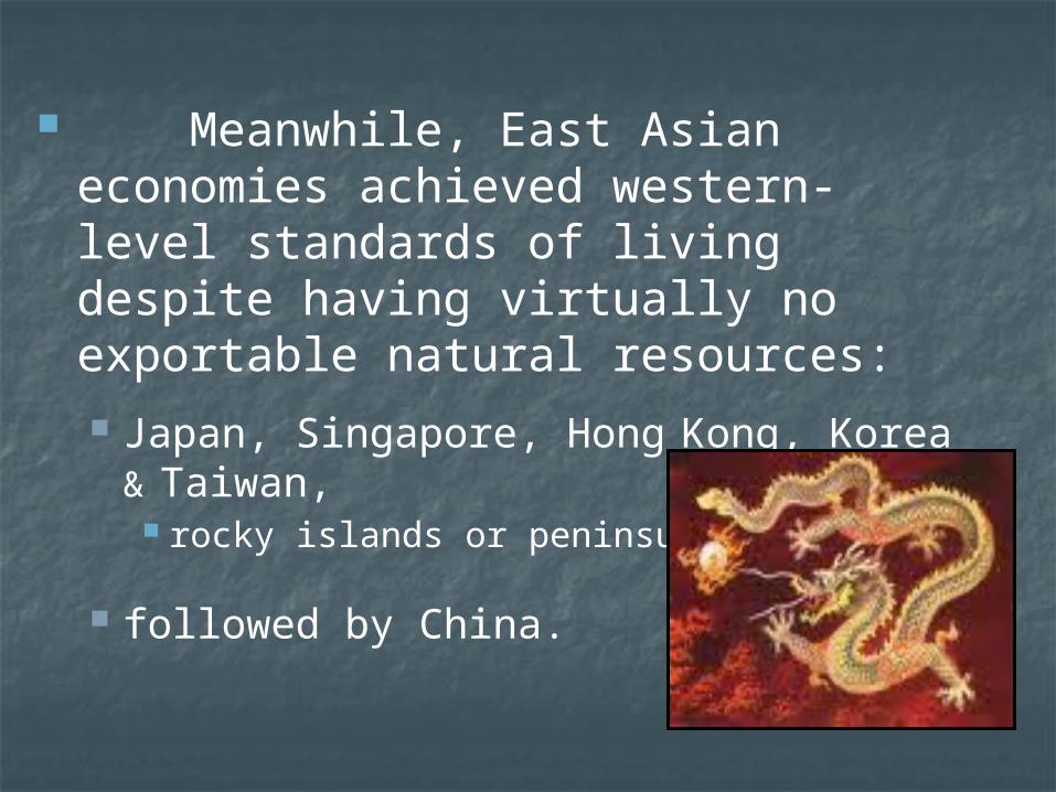
Meanwhile, East Asian economies achieved western-level standards of living despite having virtually no exportable natural resources: Japan, Singapore, Hong Kong, Korea &
Taiwan, rocky islands or peninsulas;
followed by China.
6
Are natural resources necessarily bad?
Commodity wealth need not necessarily lead to inferior economic or political development.
Rather, it is a double-edged sword, with both benefits and dangers. It can be used for ill as easily as for good.
The priority should be on identifying ways to sidestep the pitfalls that have afflicted
commodity producers in the past, to find the path of success.
No, of course not.

7
Some developing countries have avoided the pitfalls of commodity wealth. E.g., Chile (copper) Botswana (diamonds)
Some of their innovations are worth emulating.
The 2nd half of the lecture will offer some policies & institutional innovations to avoid the curse:
especially ways of managing price volatility. Some lessons apply to commodity importers
too. Including lessons of policies to avoid.

8
But, 1st: How could abundance of commodity wealth be a curse?
What is the mechanism for this counter-intuitive
relationship? At least 5 categories of
explanations.

9
1. Volatility
2. Crowding-out of manufacturing
3. Autocratic Institutions
4. Anarchic Institutions
5. Procyclicality including
1. Procyclical capital flows2. Procyclical monetary policy3. Procyclical fiscal policy.
5 Possible Natural Resource Curse Channels
10
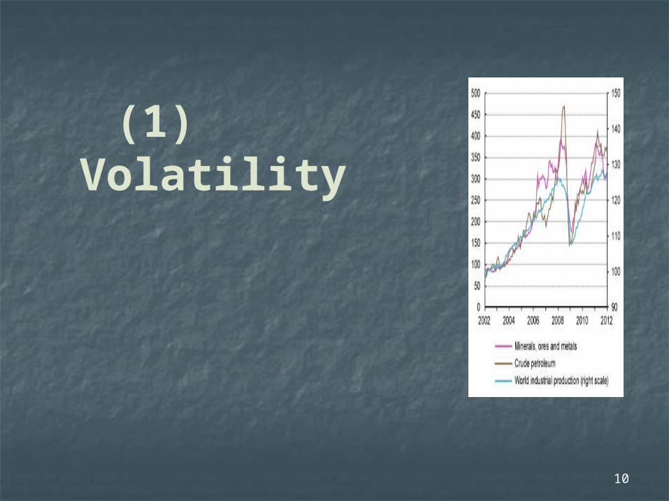
(1) Volatility

11
Effects of Volatility
Volatility per se can be bad for economic growth.
Hausmann & Rigobon (2003), Blattman, Hwang, & Williamson (2007), and Poelhekke & van der Ploeg (2007).
Risk inhibits private investment. Cyclical shifts of labor, land & capital back
& forth across sectors may incur needless costs.
=> role for government intervention? On the one hand, the private sector dislikes risk
as much as government does & takes steps to mitigate it.
On the other hand the government cannot entirely ignore the issue of volatility;
e.g., exchange rate policy.

2. Natural resources may crowd out
manufacturing, and manufacturing could be the sector
that experiences learning-by-doing or dynamic productivity gains from spillover. Matsuyama (1992), van Wijnbergen (1984) and Sachs & Warner
(1995).
So commodities could in theory be a dead-end sector.
My own view: a country need not repress the commodity sector to develop the manufacturing
sector. It can foster growth in both .
E.g. Canada, Australia, Norway… Now Malaysia, Chile, Brazil…

Econometric findings that oil
and other “point-source resources” lead to poor institutions
Isham, Woolcock, Pritchett, & Busby (2005) Sala-I-Martin & Subramanian (2003) Bulte, Damania & Deacon (2005) Mehlum, Moene & Torvik (2006) Arezki & Brückner (2009).

What are poor institutions?
A typical list: inequality, corruption, rent-seeking, intermittent dictatorship, ineffective judiciary branch, and lack of constraints to prevent elites & politicians from plundering the country.

An example, from economic
historians Engerman & Sokoloff (1997, 2000, 2002)
Why did industrialization take place in North America, not the South?
Lands endowed with extractive industries & plantation crops developed slavery, inequality, dictatorship, and state control,
whereas those climates suited to small farms & fishingdeveloped institutions of individualism, democracy, egalitarianism & capitalism.
When the Industrial Revolution came, the latter areas were well-suited to make the most of it.
Those that had specialized in extractive industries were not, because society had come to depend on class structure &
authoritarianism, rather than on individual incentive & decentralized decision-making.

16
4. Anarchic institutions
1. Unsustainably rapid depletion of resources
2. Unenforceable property rights
3. Civil war
See Appendix 2 for elaboration on each.

17
(5) Procyclicality The Dutch Disease describes unwanted
side-effects of a commodity boom.
Developing countries are historically prone to procyclicality, especially commodity producers.
Procyclicality in: Capital inflows; Monetary policy; Real exchange rate; Nontraded Goods Fiscal Policy

18
The Dutch Disease: 5 side-effects of a commodity
boom
1) A real appreciation in the currency
2) A rise in government spending 3) A rise in nontraded goods
prices
4) A resultant shift of production out of manufactured goods
5) Sometimes a current account deficit

19
The Dutch Disease: The 5 effects elaborated
1) Real appreciation in the currency
taking the form of nominal currency appreciation if the exchange rate floats
or the form of money inflows, credit & inflation if the exchange rate is fixed;
2) A rise in government spending in response to availability of tax receipts or royalties.

20
The Dutch Disease: 5 side-effects of a commodity boom
3) An increase in nontraded goods prices relative to internationally traded goods
4) A resultant shift out of non-commodity traded goods,
esp. manufactures,
pulled by the more attractive returns in the export commodity and in non-traded goods.

21
The Dutch Disease: 5 side-effects of a commodity boom
5) A current account deficit, as booming countries attract capital flows,
thereby incurring international debt that is hard to service when the boom ends.
Manzano & Rigobon (2008): the negative Sachs-Warner effect of resources on growth rates during 1970-1990 was mediated through international debt incurred when commodity prices were high.
Arezki & Brückner (2010a, b): commodity price booms lead to higher government spending, external debt & default risk in autocracies,
but do not have those effects in democracies.

Procyclical capital flows According to intertemporal optimization theory,
capital flows should be countercyclical: net capital inflows when exports are doing badly and net capital outflows when exports do well.
In practice, it does not always work this way. Capital flows are more procyclical than countercyclical. Gavin, Hausmann, Perotti & Talvi (1996); Kaminsky, Reinhart &
Vegh (2005); Reinhart & Reinhart (2009); and Mendoza &
Terrones (2008).
Invalidates much of existing theory, though certainly not all. Theories to explain this involve
capital market imperfections, e.g., asymmetric information or the need for collateral.
Procyclical monetary policy
If the exchange rate is fixed, surpluses during commodity booms
lead to rising reserves & money supply. possibly delayed by sterilization attempts.
Example: Gulf States during recent oil booms.
Floating can help, accommodating trade shock. But,
under pure floating: appreciation can be excessive. under IT: CPI rule says to tighten money & appreciate
when import commodity price goes up (or other adverse supply shock).
That’s backwards. (E.g., oil importers in 2008.) Should appreciate when export commodity price goes
up.

Procyclical real exchange rateCountries undergoing a commodity
boom experience real appreciation of their currency
taking the form of nominal currency appreciation
for floating-rate commodity exporters, Colombia, Kazakhstan, Russia, S.Africa, Chile, Brazil….
or the form of money inflows & inflation for fixed-rate commodity exporters,
Saudi Arabia & UAE….OK. But real appreciation adds to boom in NTGs.

Procyclical fiscal policy
Fiscal policy has historically tended to be procyclical in developing countries especially among commodity exporters: Cuddington (1989), Tornell & Lane (1999), Kaminsky,
Reinhart & Vegh (2004), Talvi & Végh (2005), Alesina, Campante & Tabellini (2008), Mendoza & Oviedo (2006), Ilzetski & Vegh (2008), Medas & Zakharova (2009), Gavin & Perotti (1997).
Correlation of income & spending mostly
positive – particularly in comparison with industrialized countries.

26
The procyclicality of fiscal policy
A reason for procyclical public spending: receipts from taxes & royalties rise in booms.
The government cannot resist the temptation to increase spending proportionately, or more.
Then it is forced to contract in recessions, thereby exacerbating the swings.
27
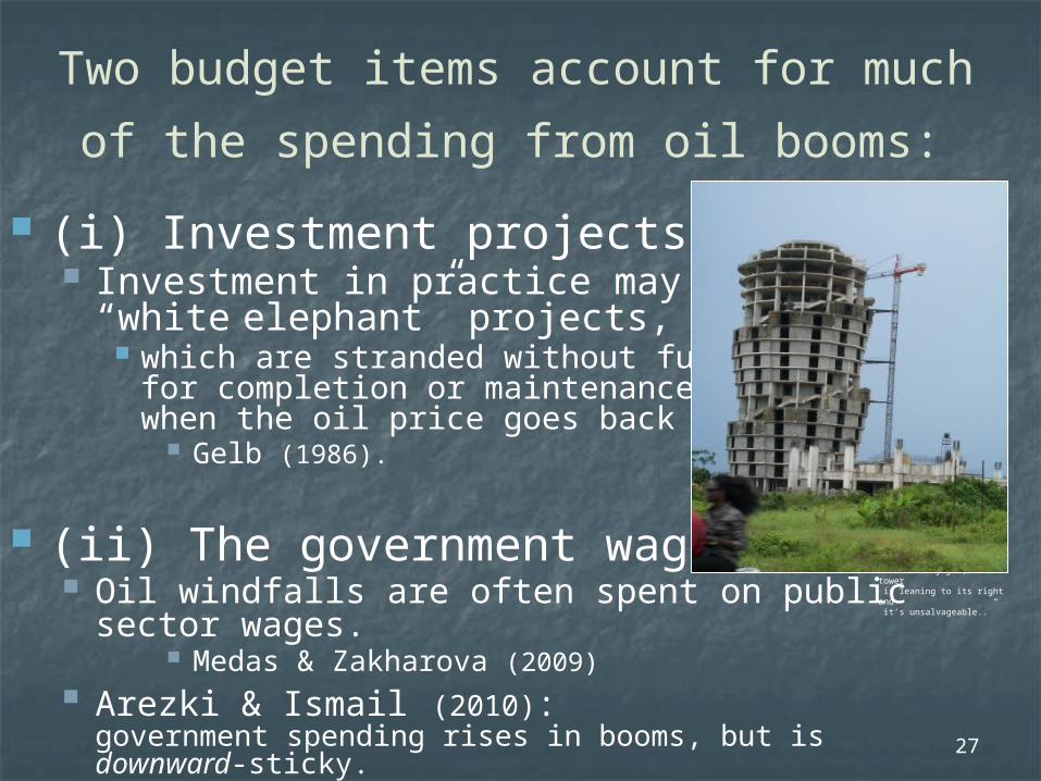
Two budget items account for much
of the spending from oil booms: (i) Investment projects.
Investment in practice may be “white elephant” projects,
which are stranded without funds for completion or maintenance when the oil price goes back down.
Gelb (1986).
(ii) The government wage bill. Oil windfalls are often spent on public sector
wages. Medas & Zakharova (2009)
Arezki & Ismail (2010): government spending rises in booms, but is downward-sticky.
Rumbi Sithole took this photo in “Bayelsa Statein the Niger Delta,in Nigeria.
The state government received a windfall of money and didn't have the capacity to have it all absorbed in social services so they decided to build a Hilton Hotel. The construction company did a shoddy job, so the tower is leaning to its right and it’s unsalvageable..”

Correlations between Gov.t Spending & GDP1960-1999
pro
cyc
lical }
G always used to be pro-cyclical for most developing countries.
cou
nte
rcyc
lical
Adapted from Kaminsky, Reinhart & Vegh (2004)

29
An important development -- some developing countries, including commodity producers, were able to break
the historic pattern in the most recent decade: taking advantage of the boom of 2002-2008
to run budget surpluses & build reserves, thereby earning the ability to expand
fiscally in the 2008-09 crisis. Chile is the outstanding model.
Also Botswana, China, Indonesia, Korea…
The procyclicality of fiscal policy, cont.

Correlations between Government spending & GDP 2000-2009
In the last decade, about 1/3 developing countries
switched to countercyclical fiscal policy:Negative correlation of G & GDP.
Frankel, Vegh & Vuletin (2012)
pro
cyc
lical
cou
nte
rcyc
lical

Summary of NRC, Part I Five broad categories of hypothesized channels
whereby natural resources can lead to poor economic performance: commodity price volatility, crowding out of manufacturing, autocratic institutions, anarchic institutions, and procyclical macroeconomic policy, including
capital flows, monetary policy and fiscal policy.
But the important question is how to avoid the pitfalls, to achieve resource blessing instead of resource
curse.

32

Appendix 1: I exclude a 6th channel,
The Prebisch-Singer (1950) Hypothesis
that commodities supposedly suffer a long-run downward relative price trend. Theoretical reasoning: world demand for
primary products is inelastic with respect to income.
Vs. persuasive theoretical arguments that we should expect commodity prices to show upward trends in the long run Malthus (esp. for food) Hotelling (for depletable resources).
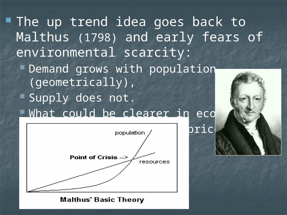
The up trend idea goes back to Malthus (1798) and early fears of environmental scarcity: Demand grows with population
(geometrically), Supply does not. What could be clearer in economics than the prediction that price will rise?

Hotelling (1931)
Firms choose how fast to extract oil or minerals King Abdullah of Saudi Arabia, with interest rates ≈ 0
in 2008, apparently believed that the rate of return on oil reserves was higher if he didn't pump than if he did:
"Let them remain in the ground for our children and grandchildren..."
Arbitrage => expected rate of price increase = interest
rate.

The empirical evidence
With strong theoretical arguments on both sides, either for an upward trend or for a downward trend, it is an empirical question.
Terms of trade for commodity producers had a slight up trend from 1870 to World War I, a down trend in the inter-war period, up in the 1970s, down in the 1980s and 1990s, and up in the first decade of the 21st
century.

What is the overall statistical trend
in commodity prices in the long run?
Some authors find a slight upward trend, some a slight downward trend. [1]
The answer depends on the date of the end of the sample.
[1] Cuddington (1992), Cuddington, Ludema & Jayasuriya (2007), Cuddington & Urzua (1989), Grilli & Yang (1988), Pindyck (1999), Reinhart & Wickham (1994), Hadass & Williamson (2003), Kellard & Wohar (2005), Balagtas & Holt (2009), Cuddington & Jerrett (2008), and Harvey, Kellard, Madsen & Wohar (2010).

38
4.1 Unsustainably rapid depletion When exhaustible resources
are in fact exhausted, the country may be left with nothing.
Three concerns: Protection of environmental quality. A motivation for a strategy of economic
diversification. The need to save for the day of depletion
Invest rents from exhaustible resources in other assets. Hartwick (1977) and Solow (1986).
Appendix 2: Elaboration on Anarchy:insufficient protection of property rights

The example of Nauruphosphate mining

40
4.2 Unenforceable property rights
Depletion would be much less of a problem if full property rights could be enforced, thereby giving the owners incentive
to conserve the resource in question.
But often this is not possible especially under frontier conditions.
Overfishing, overgrazing, & over-logging are classic examples of the “tragedy of the commons.”
Individual fisherman, ranchers, loggers, or miners,
have no incentive to restrain themselves, while the fisheries, pastureland or forests are collectively depleted.

Madre de Dios region of the Amazon rainforest in Peru,
the left-hand side stripped by illegal gold mining.
http://indiancountrytodaymedianetwork.com/2011/02/27/amazon-gold-rush-laying-waste-to-peruvian-rainforest%E2%80%99s-madre-de-dios-20021
42
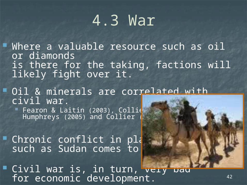
4.3 War Where a valuable resource such as oil or
diamonds is there for the taking, factions will likely fight over it.
Oil & minerals are correlated with civil war. Fearon & Laitin (2003), Collier & Hoeffler (2004),
Humphreys (2005) and Collier (2007).
Chronic conflict in places such as Sudan comes to mind.
Civil war is, in turn, very bad for economic development.

Appendix 3:The NRC Skeptics
Which comes first, oil or institutions?
Some question the assumption that oil discoveries are exogenous and institutions endogenous.
Oil wealth is not necessarily the cause and institutions the effect, rather than the other way around. Norman (2009): the discovery & development of oil
is not purely exogenous, but rather is endogenous with respect to the efficiency of the economy.

in which case it is put to use for the national
welfare, instead of the welfare of an elite.
Mehlum, Moene & Torvik (2006), Robinson, Torvik & Verdier (2006), McSherry (2006), Smith (2007) and Collier & Goderis (2007).
The important determinant is whether the country already has good
institutions at the time that oil is discovered,

Skeptics argue that commodity exports are endogenous.
On the one hand, basic trade theory says:A country may show a high mineral share in exports, not necessarily because it has a higher endowment of minerals than others (absolute advantage) but because it does not have the ability to export manufactures (comparative advantage).
This could explain negative statistical correlations between mineral exports and economic development, invalidating the common inference that minerals are bad for
growth.
Maloney (2002) and Wright & Czelusta (2003, 04, 06).

Commodity exports are endogenous, continued.
On the other hand, skeptics also have plenty of examples where successful institutions and industrialization went hand in hand with rapid development of mineral resources.
Countries that were able to develop efficiently their resource endowments as part of strong economy-wide growth include: the USA during its pre-war industrialization period
David & Wright (1997).
Venezuela from the 1920s to the 1970s, Australia since the 1960s, Norway since 1969 oil discoveries, Chile since adoption of a new mining code in 1983, Peru since a privatization program in 1992, and Brazil since lifting restrictions on foreign mining participation in 1995.
Wright & Czelusta (2003, pp. 4-7, 12-13, 18-22).

Commodity exports are endogenous, continued.
Examples of countries that were equally well-endowed geologically but that failed to develop their natural resources efficiently include:
Chile & Australia before World War I,
and Venezuela since the 1980s. Hausmann (2003, p.246): “Venezuela’s growth collapse
took place after 60 years of expansion, fueled by oil. If oil explains slow growth, what explains the previous fast growth?”

Addendum: Countries with high resource
revenuetend to have high government spending (as
% of GDP)
48
IMF blogJune 9, 2014

But countries with high resource rents (as % of GDP)
tend to have lower student math performance(statistically significant at the .003 level)
49
Source: OECD education data featured in Knowledge and skills are infinite – oil is not by Andreas Schleicher.

Part II
Some that are not recommended: Institutions that try to suppress price
volatility.
Recommended: Devices to hedge risk. Ideas to reduce macroeconomic
procyclicality. Institutions for better governance.
Policies & institutions to avoidpitfalls of the Natural Resource
Curse
52
The Natural Resource Curse should not be interpreted as a rule that
commodity-rich countries are doomed to fail.
The question is what policies to adopt to avoid the pitfalls and improve the chances of
prosperity. A wide variety of measures have been tried by commodity-exporters cope with volatility.
Some work better than others.

Many of the policies that have been intended to suppress
commodity volatility do not work out so well
Producer subsidies Stockpiles Marketing boards Price controls Export controls
Blaming derivatives
Resource nationalism
Nationalization Banning foreign
participation
Devices to share risks
1. Index contracts with foreign companies(royalties…) to the world commodity price.
2. Hedge commodity revenues in options markets
3. Link debt to the commodity price
7 recommendations for commodity-exporting countries

4. Allow some currency appreciation in response to a commodity boom, but not a free float. - Accumulate some forex reserves first.- Raise banks’ reserve requirements, esp. on $ liabilities.
5. If the monetary anchor is to be Inflation Targeting, consider using as the target, in place of the CPI, a measure that puts weight on the export commodity.
6. Emulate Chile: to avoid over-spending in boom times, allow deviations from a target surplus only in response to permanent commodity price rises.
7 recommendations for commodity producers continued
Countercyclical macroeconomic policy
PPT

7. Manage commodity funds professionally.
Invest them abroad like Norway’s Pension Fund, Reasons:
(1) for diversification, (2) to avoid cronyism in investments.
but insulated from politics like Botswana’s Pula Fund. Professionally managed, to optimize financially.
7 recommendations for commodity producers, concluded
Good governance institutions
Elaboration on two proposals to reduce the procyclicality of
macroeconomic policy for commodity exporters
I) To make monetary policy less procyclical: Product Price Targeting
II) To make fiscal policy less procyclical: emulate Chile.
PPT

I) The challenge of designinga currency regime for countries where
terms of trade shocks dominate the cycle
Fixing the exchange rate leads to procyclical monetary policy: credit expands in commodity booms.
Floating accommodates terms of trade shocks. But volatility can be excessive; also floating does not provide a nominal anchor.
Inflation Targeting, in terms of the CPI, provides a nominal anchor; but can react perversely to terms of trade shocks.
Needed: an anchor that accommodates trade shocks

Product Price Targeting:Target an index of domestic production
prices [1]
such as the GDP deflator
• Include export commodities in the index and exclude import commodities,
• so money tightens & the currency appreciates when world prices of export commodities rise
• accommodating the terms of trade --• not when world prices of import commodities
rise.
• The CPI does it backwards:• It calls for appreciation when import prices rise,• not when export prices rise !
[1] Frankel (2011, 2012).
PPT

Appendix II: Who achieves counter-cyclical fiscal
policy?Countries with “good institutions”
”On Graduation from Fiscal Procyclicality” 2013, Frankel with C.Végh & G.Vuletin; J.Dev.Economics.

What, specifically, are good institutions?
1st rule – Governments must set a budget target,
set = 0 in 2008 under Pres. Bachelet.
2nd rule – The target is structural: Deficits allowed only to the extent that (1) output falls short of trend, in a recession, or (2) the price of copper is below its trend.
3rd rule – The trends are projected by 2 panels of independent experts, outside the political process. Result: Chile avoids the pattern of 32 other
governments, where forecasts in booms are biased toward over-
optimism. Chile ran surpluses in the 2003-07 boom,
while the U.S. & Europe failed to do so.
The example of Chile since 2000

Appendiceson recommendations for
dealing with the natural resource curse
Appendix 4: Policies not recommended
Appendix 5: Elaboration on proposal to make monetary policy less procyclical – PPT, using GDP deflator to set annual inflation target.
Appendix 6: Elaboration on proposal to make fiscal policy less procyclical – emulate Chile, setting structural targets with independent fiscal forecasts
Appendix 4: Policies that have been
triedbut that are not recommended
Producer subsidies Stockpiles Marketing boards Price controls Export controls
Blaming derivatives
Resource nationalism
Nationalization Banning foreign
participation

Unsuccessful policies to reduce commodity price volatility:
1) Producer subsidies to “stabilize” prices at high levels, often via wasteful stockpiles & protectionist import
barriers.
Examples: The EU’s Common Agricultural Policy
Bad for EU budgets, economic efficiency, international trade & consumer pocketbooks.
Or fossil fuel subsidies which are equally distortionary & budget-busting, and disastrous for the environment as well.
Or US corn-based ethanol subsidies, with tariffs on Brazilian sugar-based ethanol.

Unsuccessful policies, continued
2) Price controls to “stabilize” prices at low levels Discourage investment & production.
Example: African countries adopted commodity boards for coffee & cocoa at the time of independence.
The original rationale: to buy the crop in years of excess supply and sell in years of excess demand.
In practice the price paid to cocoa & coffee farmers
was always below the world price. As a result, production fell.

Microeconomic policies, continued
Often the goal of price controls is to shield consumers of staple foods & fuel from increases. But the artificially suppressed price
discourages domestic supply, and requires rationing to domestic households.
Shortages & long lines can fuel political rage as well as higher prices can.
Not to mention when the government is forced by huge gaps to raise prices.
Price controls can also require imports, to satisfy excess demand.
Then they raise the world price even more.

Microeconomic policies, continued
3) In producing countries, prices are artificially suppressed by means of export controls to insulate domestic consumers from a price
rise. In 2008, India capped rice exports. Argentina did the same for wheat exports, as did Russia in 2010. India banned cotton exports in March2012.
Results: Domestic supply is discouraged. World prices go even higher.

An initiative at the G20 meetings in
France in 2011 deserved
to succeed: Producers and consuming countries in
grain markets should cooperatively agree to refrain from export controls and price controls. The result would be lower world price
volatility. One hopes for steps in this direction,
perhaps working through the WTO.

An initiative that has less merit:
4) Attempts to blame speculation for volatility and so to ban derivatives markets.
Yes, speculative bubbles sometimes hit prices.
But in commodity markets, prices are more often the signal for
fundamentals. Don’t shoot the messenger.
Also, derivatives are useful for hedgers.

The overall lesson for microeconomic policy
Attempts to prevent commodity prices from fluctuating generally fail.
Even though enacted in the name of reducing volatility & income inequality, their effect is often different.
Better to accept volatility and cope with it.
For the poor: well-designed transfers, along the lines of Oportunidades or Bolsa Familia.
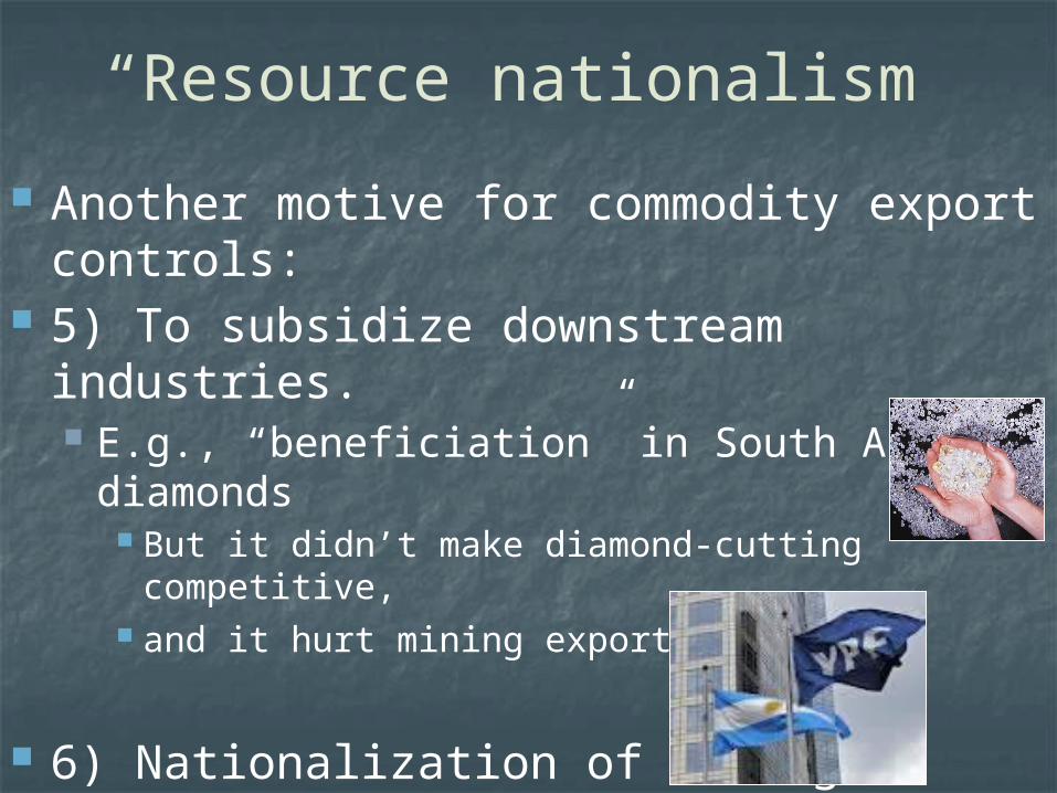
“Resource nationalism”
Another motive for commodity export controls:
5) To subsidize downstream industries. E.g., “beneficiation” in South African
diamonds But it didn’t make diamond-cutting competitive, and it hurt mining exports.
6) Nationalization of foreign companies. Like price controls,
it discourages investment.

“Resource nationalism” continued
7) Keeping out foreign companies altogether. But often they have the needed technical expertise. Examples: declining oil production in Mexico &
Venezuela.
8) Going around “locking up” resource supplies. China must think that this strategy will
protect it in case of a commodity price shock. But global commodity markets are increasingly
integrated. If conflict in the Persian Gulf doubles world oil prices,
the effect will be pretty much the same for those who buy on the spot market and those who have bilateral arrangements.

The overall lesson for microeconomic policy
Attempts to prevent commodity prices from fluctuating generally fail.
Even though enacted in the name of reducing volatility & income inequality, their effect is often different.
Better to accept volatility and cope with it. For the poor: well-designed transfers,
along the lines of Oportunidades or Bolsa Familia.

Appendix 5: Product Price Targeting
Each of the traditional candidates for nominal anchor has an Achilles heel.
The CPI anchor does not accommodate terms of trade changes: IT tightens M & appreciates when import
prices rise not when export prices rise, which is backwards. Targeting core CPI does not much help.

Professor Jeffrey Frankel
Targeted variable
Vulnerability Example
Gold standard
Price of gold
Vagaries of world gold market
1849 boom; 1873-96 bust
Commodity standard
Price of agric. & mineral
basket
Shocks in imported
commodity
Oil shocks of 1973-80, 2000-11
Monetarist rule M1 Velocity shocks US 1982
Nominal income targeting
Nominal GDP
Measurement problems
Less developed countries
Fixed exchange rate
$ (or €)
Appreciation of $ (or € )
EM currency crises 1995-2001
Inflation targeting CPI
Terms of trade shocks
Oil shocks of 1973-80, 2000-11
6 proposed nominal targets and the Achilles heel of each:Vulnerability

Why is PPT better than a fixed exchange ratefor countries with volatile export prices?
Better response to trade shocks (countercyclical):
If the $ price of the export commodity goes up, the currency automatically appreciates, moderating the boom.
If the $ price of the export commodity goes down, the currency automatically depreciates, moderating the downturn & improving the balance of payments.
PPT
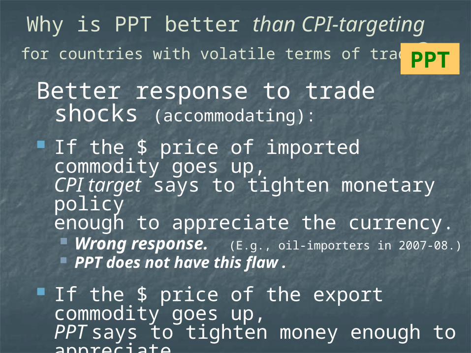
Why is PPT better than CPI-targetingfor countries with volatile terms of trade?
Better response to trade shocks (accommodating):
If the $ price of imported commodity goes up, CPI target says to tighten monetary policy enough to appreciate the currency. Wrong response. (E.g., oil-importers in 2007-08.) PPT does not have this flaw .
If the $ price of the export commodity goes up, PPT says to tighten money enough to appreciate. Right response. (E.g., Gulf currencies in 2007-08.) CPI targeting does not have this advantage.
PPT

Empirical findings
Simulations of 1970-2000 Gold producers:
Burkino Faso, Ghana, Mali, South Africa Other commodities:
Ethiopia (coffee), Nigeria (oil), S.Africa (platinum)
General finding: Under Product Price Targets, their currencies would have depreciated automatically in 1990s when commodity prices declined,
perhaps avoiding messy balance of payments crises.
Sources: Frankel (2002, 03a, 05), Frankel & Saiki (2003)
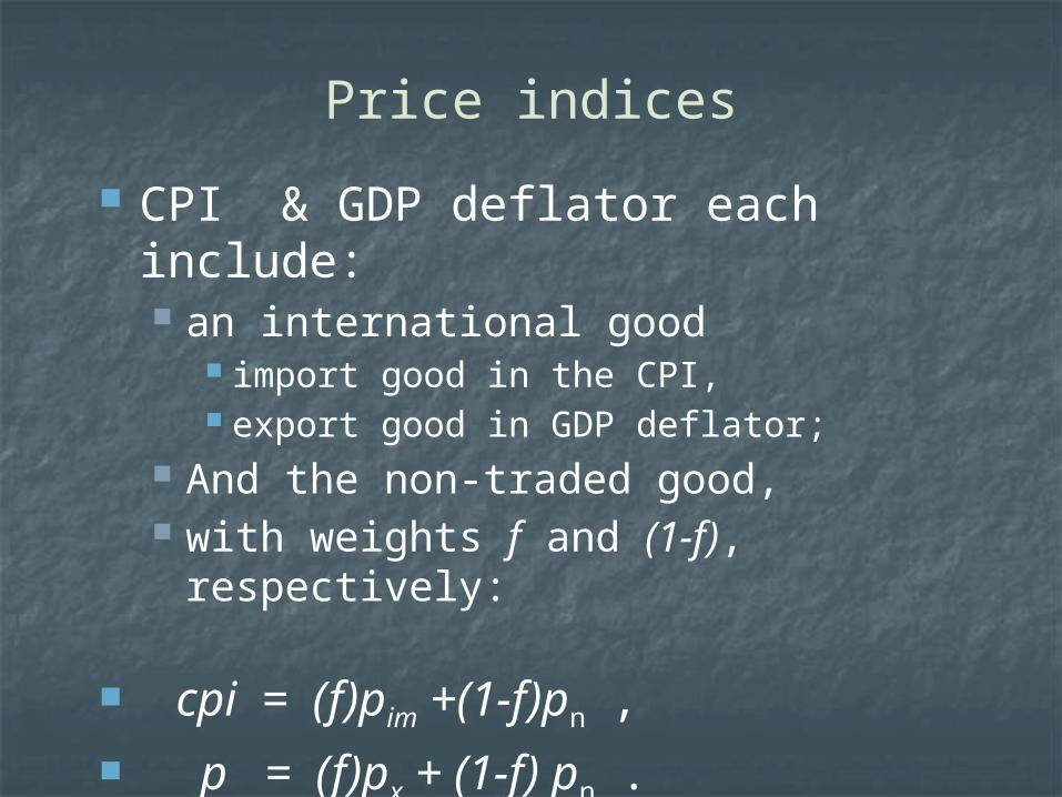
Price indices
CPI & GDP deflator each include: an international good
import good in the CPI, export good in GDP deflator;
And the non-traded good, with weights f and (1-f), respectively:
cpi = (f)pim +(1-f)pn , p = (f)px + (1-f) pn .

Estimation for each country of weights in national price index on 3 sectors: non tradable goods, leading commodity export, & other tradable goods
Non Tradables
Leading Comm. Export
OilOther
TradablesTotal
CPI 0.6939 0.0063 0.0431 0.2567 1.000PPI 0.6939 0.0391 0.0230 0.2440 1.000CPI 0.5782 0.0163 0.0141 0.3914 1.000PPI 0.5782 0.1471 0.0235 0.2512 1.000CPI 0.5235 0.0079 0.0608 0.4078 1.000PPI 0.5235 0.0100 0.1334 0.3332 1.000CPI 0.5985 -- 0.0168 0.3847 1.000PPI 0.5985 -- 0.0407 0.3608 1.000CPI 0.6413 0.0002 0.0234 0.3351 1.000PPI 0.6413 0.1212 0.0303 0.2072 1.000CPI 0.3749 -- 0.0366 0.5885 1.000PPI 0.3749 -- 0.0247 0.6003 1.000CPI 0.3929 0.1058 0.0676 0.4338 1.000PPI 0.3929 0.0880 0.0988 0.4204 1.000CPI 0.6697 0.0114 0.0393 0.2796 1.000PPI 0.6697 0.040504 0.021228 0.268568 1.000CPI 0.6230 0.0518 0.0357 0.2895 1.000PPI 0.6230 0.2234 0.1158 0.0378 1.000
* Oil is the leading commodity export.
PRY
PER
URY
ARG
BOL
CHL
COL*
JAM
MEX*
Argentina is relatively closed;
The leading export commodity usually has a higher weight in the country’s PPI
than in its CPI, as expected.
(Jamaicans don’t eat bauxite.)
Mexico is relatively open.
“A Comparison of Product Price Targeting and Other Monetary Anchor Options, for Commodity-Exporters in Latin America," Economia, vol.11, 2011 (Brookings), NBER WP 16362.

In practice, IT proponents agree central banks should not tighten to offset oil price
shocks
They want focus on core CPI, excluding food & energy.
But food & energy ≠ all supply shocks.
Use of core CPI sacrifices some credibility: If core CPI is the explicit goal ex ante, the public feels
confused. If it is an excuse for missing targets ex post, the public feels
tricked.
Perhaps for that reason, IT central banks apparently do respond to oil shocks by tightening/appreciating,
as the following correlations suggests….

Table 1: LACA Countries’ Current Regimes and Monthly Correlations of Exchange Rate Changes ($/local currency) with Dollar Import Price Changes
Import price changes are changes in the dollar price of oil.
Exchange Rate Regime Monetary Policy 1970-1999 2000-2008 1970-2008
ARG Managed floating Monetary aggregate target -0.0212 -0.0591 -0.0266
BOL Other conventional fixed peg Against a single currency -0.0139 0.0156 -0.0057
BRA Independently floating Inflation targeting framework (1999) 0.0366 0.0961 0.0551
CHL Independently floating Inflation targeting framework (1990)* -0.0695 0.0524 -0.0484
CRI Crawling pegs Exchange rate anchor 0.0123 -0.0327 0.0076
GTM Managed floating Inflation targeting framework -0.0029 0.2428 0.0149
GUY Other conventional fixed peg Monetary aggregate target -0.0335 0.0119 -0.0274
HND Other conventional fixed peg Against a single currency -0.0203 -0.0734 -0.0176
JAM Managed floating Monetary aggregate target 0.0257 0.2672 0.0417
NIC Crawling pegs Exchange rate anchor -0.0644 0.0324 -0.0412
PER Managed floating Inflation targeting framework (2002) -0.3138 0.1895 -0.2015
PRY Managed floating IMF-supported or other monetary program -0.023 0.3424 0.0543
SLV Dollar Exchange rate anchor 0.1040 0.0530 0.0862
URY Managed floating Monetary aggregate target 0.0438 0.1168 0.0564
Oil Exporters
COL Managed floating Inflation targeting framework (1999) -0.0297 0.0489 0.0046
MEX Independently floating Inflation targeting framework (1995) 0.1070 0.1619 0.1086
TTO Other conventional fixed peg Against a single currency 0.0698 0.2025 0.0698
VEN Other conventional fixed peg Against a single currency -0.0521 0.0064 -0.0382
* Chile declared an inflation target as early as 1990; but it also had an exchange rate target, under an explicit band-basket-crawl regime, until 1999.
LAC Countries’ Current Regimes and Monthly Correlations of Exchange Rate Changes ($/local currency) with $ Import Price Changes
Table 1
ITcoun-triesshowcorrel-ations> 0.

The 4 inflation-targeters in Latin America
show correlation (currency value in $ , import prices in $) > 0 ;
> correlation before they adopted IT;
> correlation shown by non-IT Latin American oil-importing countries.

Why is the correlation between the import price and the currency value
revealing?
The currency of an oil importer should not respond to an increase in the world oil price by appreciating, to the extent that these central banks target core CPI .
When these IT currencies respond by appreciating instead, it suggests that the central bank is tightening money to reduce upward pressure on headline CPI.

Appendix 6: Chilean fiscal policy
In 2000 Chile instituted its structural budget rule.
The institution was formalized in law in 2006.
The structural budget deficit must be zero, originally BS > 1% of GDP, then cut to ½ %, then 0 -- where structural is defined by output & copper price
equal to their long-run trend values.
I.e., in a boom the government can only spend increased revenues that are deemed permanent; any temporary copper bonanzas must be saved.
The crucial institutional innovation in Chile
How has Chile avoided over-optimistic official forecasts? especially the historic pattern of
over-exuberance in commodity booms?
The estimation of the long-term path for GDP & the copper price is made by two panels of independent experts, and thus is insulated from political pressure & wishful thinking.
Other countries might usefully emulate Chile’s innovation or in other ways delegate to independent agencies
estimation of structural budget deficit paths.

Chile’s fiscal position strengthened immediately: Public saving rose from 2.5 % of GDP in 2000 to 7.9 % in 2005 allowing national saving to rise from 21 % to 24 %.
Government debt fell sharply as a share of GDP and the sovereign spread gradually declined.
By 2006, Chile achieved a sovereign debt rating of A, several notches ahead of Latin American peers.
By 2007 it had become a net creditor. By 2010, Chile’s sovereign rating had climbed to A+,
ahead of some advanced countries.
=> It was able to respond to the 2008-09 recession via fiscal expansion.
The Pay-off

In 2008, with copper prices spiking up, the government of President Bachelet had beenunder intense pressure to spend the revenue. She & Fin.Min.Velasco held to the rule, saving most of it. Their popularity ratings fell sharply.
When the recession hit and the copper price came back down, the government increased spending, mitigating the downturn. Bachelet & Velasco’s
popularity reached historic highs in 2009.

Evolution of approval and disapproval of four Chilean presidents
Presidents Patricio Aylwin, Eduardo Frei, Ricardo Lagos and Michelle BacheletData: CEP, Encuesta Nacional de Opinion Publica, October 2009, www.cepchile.cl. Source: Engel et al (2011).

5 econometric findings regarding bias toward optimism in official budget forecasts.
Official forecasts in a sample of 33 countries on average are overly optimistic, for:
(1) budgets & (2) GDP .
The bias toward optimism is: (3) stronger the longer the forecast horizon; (4) greater in booms (5) greater for euro governments under SGP budget rules;
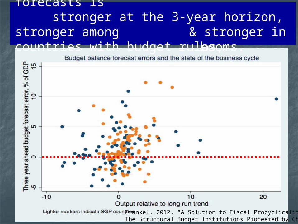
(4) The optimism in official budget forecasts is stronger at the 3-year horizon, stronger amongcountries with budget rules, & stronger in booms.
Frankel, 2012, “A Solution to Fiscal Procyclicality: The Structural Budget Institutions Pioneered by Chile.”

Budget balance forecast error as % of GDP, Full dataset
(1) (2) (3)
One year ahead Two years ahead Three years ahead
GDP relative to trend
0.093***(0.019)
0.258***(0.040)
0.289***(0.063)
Constant 0.201 0.649*** 1.364***(0.197) (0.231) (0.348)
Observations 398 300 179Variable is lagged so that it lines up with the year in which the forecast was made.*** p<0.01 Robust standard errors in parentheses, clustered by country.
(4) Official budget forecasts are biasedmore if GDP is currently high & especially at
longer horizons
33 countries

Budget balance forecast error as a % of GDP, Full Dataset
(1) (2) (3) (4)
One year ahead
Two years ahead
One year ahead
Two years ahead
SGPdummy 0.658 0.905** 0.407 0.276(0.398) (0.406) (0.355) (0.438)
SGP dummy * (GDP - trend)
0.189**(0.0828)
0.497***(0.107)
Constant 0.033 0.466* 0.033 0.466*(0.228) (0.248) (0.229) (0.249)
Observations 399 300 398 300
(5) Official budget forecasts are more optimistically biasedin countries subject to a budget deficit rule (SGP)
*** p<0.01, ** p<0.05, * p<0.1 Robust standard errors in parentheses, clustered by country.
33 countries

5 more econometric findings regarding bias toward optimism in official budget forecasts.
(6) The key macroeconomic input for budget forecasting in most countries: GDP. In Chile: the copper price.
(7) Real copper prices revert to trend in the long run.
But this is not always readily perceived: (8) 30 years of data are not enough
to reject a random walk statistically; 200 years of data are needed.
(9) Uncertainty (option-implied volatility) is higher when copper prices are toward the top of the cycle.
(10) Chile’s official forecasts are not overly optimistic.It has apparently avoided the problem of forecasts that unrealistically extrapolate in boom times.

In sum, institutions recommended to make fiscal policy less procyclical:
Official growth & budget forecasts tend toward wishful thinking : unrealistic extrapolation of booms 3 years into the future.
The bias is worse among the European countries supposedly subject to the budget rules of the SGP, presumably because government forecasters feel pressured
to announce they are on track to meet budget targets even if they are not.
Chile is not subject to the same bias toward over-optimism in forecasts of the budget, growth, or the all-important copper price.
The key innovation that has allowed Chile to achieve countercyclical fiscal policy: not just a structural budget rule in itself, but rather the regime that entrusts to two panels of experts
estimation of the long-run trends of copper prices & GDP.
Application to other countries
Any country could adopt the Chilean mechanism.
Suggestion: give the panels more institutional independence as is familiar from central banking:
laws protecting them from being fired.
Open questions: Are the budget rules to be interpreted as ex ante or ex post? How much of the structural budget calculations are
to be delegated to the independent panels of experts? Minimalist approach: they compute only 10-year moving averages.
Can one guard against subversion of the institutions (CBO) ?

References by the author Project Syndicate,
“Escaping the Oil Curse,” Dec.9, 2011. "Barrels, Bushels & Bonds: How Commodity Exporters Can Hedge Volatility,"
Oct.17, 2011.
“The Natural Resource Curse: A Survey of Diagnoses and Some Prescriptions,” 2012, Commodity Price Volatility and Inclusive Growth in Low-Income Countries , R.Arezki & Z.Min, eds.. HKS RWP12-014. High Level Seminar, IMF Annual Meetings, DC, Sept.2011.
"The Curse: Why Natural Resources Are Not Always a Good Thing,” Milken Institute Review, vol.13, 4th quarter 2011.
“The Natural Resource Curse: A Survey,” 2012, Chapter 2 in Beyond the Resource Curse, B.Shaffer & T. Ziyadov, eds. (U.Penn. Press); proofs & notes; Summary. CID WP195, 2011.
“How Can Commodity Exporters Make Fiscal and Monetary Policy Less Procyclical?” Natural Resources, Finance & Development, R.Arezki, T.Gylfason & A.Sy, eds. (IMF), 2011. HKS RWP 11-015.
“On Graduation from Procyclicality,” 2012, with C.Végh & G.Vuletin; J. Dev. Economics.
“Chile’s Solution to Fiscal Procyclicality,” 2012, Transitions blog, Foreign Policy.
“A Solution to Fiscal Procyclicality: The Structural Budget Institutions Pioneered by Chile,” in Fiscal Policy and Macroeconomic Performance, 2012. Central Bank of Chile WP 604, 2011.
"Product Price Targeting -- A New Improved Way of Inflation Targeting," in MAS Monetary Review Vol.XI, issue 1, April 2012 (Monetary Authority of Singapore).
“A Comparison of Product Price Targeting and Other Monetary Anchor Options, for Commodity-Exporters in Latin America," Economia, vol.11, 2011 (Brookings), NBER WP 16362.